A Bifurcation Model of Non-Stationary Markets

December 2006

1

A BIFURCATION MODEL OF NON-STATIONARY MARKETS

David Nawrocki*

Villanova University

College of Commerce and Finance

800 Lancaster Avenue

Villanova, PA 19085 USA

610-519-4323

[e-mail]

Tonis Vaga

401 Linden Lane

Brielle, NJ 08730

732-528-8239

[e-mail]

* Authors are listed alphabetically. The first author is the contact person responsible for
correspondence concerning this paper.

A Bifurcation Model of Non-Stationary Markets

December 2006

2

A BIFURCATION MODEL OF NON-STATIONARY MARKETS

ABSTRACT

We propose a non-stationary model of market disequilibrium that features bifurcation of
a linear, mean regressive, equilibrium state into trend persistent coherent market states.
Empirical data covering the period between 1930 and 2005 suggests that the Dow Jones
Industrial Average has exhibited trend persistence approximately 81% of the time. Mean
regressive markets appear to follow highly volatile periods. A bifurcation dynamic is
also evident in returns conditioned on both prior day price and volume. Returns
following rising prior day volume exhibit trend persistent behavior. This finding is
consistent with prior research indicating a positive relationship between trading volume
and serial correlations for daily returns.

A Bifurcation Model of Non-Stationary Markets

December 2006

3

A BIFURCATION MODEL OF NON-STATIONARY MARKETS

INTRODUCTION

Recent studies cast doubt on the common practice of modeling stock returns or

expected returns as a constant linear function of risk. Fama and French (1989) find that

the risk premium embedded in expected returns moves inversely with business

conditions. Whitelaw (1994) reports that both expected returns and conditional volatility

move in response to the business cycle. Nawrocki (1995, 1996) and Chauvet (1998a,

1998b) propose and find a dynamic relationship between stock market fluctuations and

business cycles. Perez-Quiros and Timmermann (2000) find asymmetries in the

conditional mean and volatility of excess stock returns around business cycle turning

points. Chauvet and Potter (2000, 2001) suggest a nonlinear risk measure that allows for

the risk-return relationship to not be constant over Markov states (bull or bear) or over

time. Perez-Quiros and Timmermann (2001) also find support for a Markov switching

model with time-varying means and variances. DeStefano (2004) tests a four-state model

of the business cycle that provides additional proof that stock returns vary inversely with

economic conditions. Finally, Guidolin and Timmermann (2005) discover that a four-

state model is necessary to capture the joint distribution of US stock and bond returns.

In summary, empirical work suggests a nonlinear financial market dynamic at work,

requiring evolutionary, financial state transition models.

The application of evolutionary theory to economic processes is strongly defended by

Boulding (1981a, 1981b) and Nawrocki (1984, 1995). The use of entropy theory and

bifurcation theory is extensive in the finance and economics literature, [Murphy (1965),

Georgescu-Roegen (1971), Cozzolino and Zahner (1973), and Majthay (1980)]. Among

A Bifurcation Model of Non-Stationary Markets

December 2006

4

early research in this area, Nawrocki (1984) explores non-stationary mean jump

processes and non-stationary variability processes in the financial markets while Vaga

(1990) proposes a state transition model for the financial markets based on Weidlich

(1971), Callen and Shapero (1974) and Haken (1975).

More recently, many questions are being raised regarding the assumptions underlying

the Efficient Market Hypothesis (EMH) in Shiller (2000) and Schliefer (2000).

Alternating trending and mean reverting investor sentiment models are proposed in

Barberis, Shleifer and Vishny (1998). Hong and Stein (1999) suggest positive

correlations in returns are due to the slow dissemination of information. Wyart and

Bouchaud (2003) propose that feedback dynamics among a subset of market agents are

sufficient to create trends in anticipation of correlations. Finally Dopfer (2005) offers

unifying principles to the evolutionary approach to economics, and includes contributions

by Haken and Prigogine.

The purpose of this paper, after a brief survey of the work in financial market

disequilibrium, is to review evolutionary market state transition models and provide

additional empirical evidence in support of disequilibrium theories of the financial

markets. The structure of the paper is as follows. First, models of financial market

disequilibrium and entropy are described from the economic perspective. Next, Haken’s

general evolutionary model of state transitions is used to describe bifurcations in

undisseminated market information and conditional return states. Finally, empirical

evidence in support of the non-stationary market disequilibrium theories is presented.

FINANCIAL MARKET DISEQUILIBRIUM

A Bifurcation Model of Non-Stationary Markets

December 2006

5

The traditional tatonnement model of market equilibrium assumes a stationary

information process and an infinite speed of information dissemination in the

marketplace. The market prices that result from this process adjust immediately to new

information. Since new information is an independent process, the usual random walk

model is developed in Fama (1970).

The assumption that markets have an infinite speed of information dissemination,

however, has been questioned by a number of researchers. A developing body of

literature offers disequilibrium models of market processes. Beja and Hakansson (1977)

argue that a swift movement to a pareto-optimum price in the classical tatonnement

process is unlikely in actual security prices because of institutional rigidities such as taxes

and transaction costs. It is more likely that markets will trade at disequilibrium prices in a

search for equilibrium but will not converge to equilibrium. Grossman and Stiglitz (1976)

suggest that prices never fully adjust because of a noisy information system, the costs of

acquiring and evaluating information, and the continuing need to adjust to new

information shocks to the economy. Black (1976) argues that disequilibrium prices result

from lags in the information process.

Morse (1980) argues further that the speed of information dissemination, while

finite, is not constant, and varies with the amount of new information. With the arrival of

new information, the greater the disparity between the equilibrium price and the actual

price, the more investors want to trade, and increasing trading volume increases the

market’s speed of information dissemination. Because of the aforementioned restrictions

affecting the speed of information dissemination, greater dependence in security returns

also occurs during this period. Morse’s results indicate a positive relationship between

A Bifurcation Model of Non-Stationary Markets

December 2006

6

trading volume and serial correlations for daily data for a mixture of NYSE, AMEX and

OTC stocks.

A BIFURCATION MODEL OF MARKET DISEQUILIBRIUM

A simple bifurcation model of equilibrium states in a wide variety of systems from

various disciplines outside of finance is provided by Haken (1975) using the concept of

the damped anharmonic oscillator. Weidlich (1971) uses a similar approach to describe

states of polarized opinion in social systems. Following Haken (1975), we model the

market return, R, as:

lim

t

→0

(1/t)[R(t) – R(0)] = k [R(0)] + f [I(t), t]

(1)

where k[R(0)] = - ∑

i

a

i

R(0)

i

represents undisseminated information following a known

return, R(0) while f[I(t), t] represents random new information arrival. Setting a

0

and a

2

equal to zero, we focus on the parameters a

1

and a

3

which control the bifurcation between

a single equilibrium state to bi-stable states and the speed of the market’s information

dissemination process. Given our simplifying assumptions, Equation 1 can be expressed

as

∂R(t)/∂t = – a

1

R – a

3

R

3

+

f[I(t),

t]

(2)

With the nonlinear feedback term, – a

3

R

3

, Equation 2 is an extension of the Langevin

equation of Brownian motion. Therefore, this quantitative model of market dynamics

corresponds to the linear random walk as a special case and also allows examination of

the bifurcated equilibrium states that result from the nonlinear term. The Langevin

equation also underlies the phase transition model in Vaga (1990) and Wyart and

Bouchaud (2003).

A Bifurcation Model of Non-Stationary Markets

December 2006

7

Putting random forces f[I(t), t] = 0 for the moment, the time dependent solution to

Equation 4 has the form

R(t) = ± (a

1

)

1/2

[exp(2 a

1

t) – a

3

]

-1/2

for a

3

> 0 and a

1

> 0

(3)

and

R(t) = ± (|a

1

|)

1/2

[a

3

- exp(-2| a

1

|t)]

-1/2

for a

3

> 0 and a

1

< 0

(4)

The parameter “a

1

” can be viewed as the inverse “relaxation time” or the rate at which

the system evolves toward equilibrium as t approaches infinity. In Equation (3), there is

a single equilibrium state at R = 0, since we have arbitrarily set a

0

= 0.

In Equation (3) (when a

3

> 0 and a

1

> 0) the slope of k(R) is everywhere negative.

This implies that information dissemination causes returns to regress toward the long

term mean as new information arrives at random and creates temporary disequilibrium

states. As a

1

decreases, the slope decreases, and the speed of information dissemination

decreases and the market reacts more slowly to new information arrival. An unstable

transition occurs when a

1

= 0, a bifurcation point, where the market’s long term average

return is no longer a stable equilibrium point.

In equation (4) (when a

3

> 0 and a

1

< 0) a bifurcation results in two new equilibrium

states. Therefore, the sign of the parameter “a

1

” controls the bifurcation from a single

equilibrium state (when a

3

> 0 and a

1

> 0) into two states (when a

3

> 0 and a

1

< 0). One

new stable state is at R(bull) = + |(a

1

/a

3

)|

1/2

while the other stable state is at R(bear) = -

|(a

1

/a

3

)|

1/2

. In general, the market’s new stable states may be far from the original

A Bifurcation Model of Non-Stationary Markets

December 2006

8

equilibrium state. These states can be observed empirically by examining the conditional

return data in historical market time series.

EMPIRICAL EVIDENCE

In order to assess the validity of bifurcation model for the capital markets we examine

the correlation of daily market returns, R(t), with prior day returns, R(0). If there is a

single stable equilibrium state around the market’s long term average return (linear

random walk), the residual undisseminated information should tend to cause returns to

regress toward the long term mean. The daily mean return is 0.026% (6.7% annualized)

for the Dow Jones Industrial Average over the period from 1930 to 2005. If the market

behaves more as a bistable disequilibrium system, then the residual undisseminated

information would cause returns to drift toward either the stable bull or bear states, far

from the long term average.

Trend persistent states are clearly evident in historical conditional return data for both

the stock and bond markets. Moderate price returns tend to persist in direction, though

periods of mean regressive behavior are also evident. Historical time series analysis of

both major stock market averages and the bond market provides statistically significant

evidence of bistable financial market disequilibrium.

Dow Jones Industrial Average

The conditional returns for the DJIA from 1930 to 2005 are summarized in Table 1 for

0.5% increments between -3.75% and +3.75%. Data beyond this range are considered to

be outliers. The table summarizes the mean return, standard deviation of return, relative

frequency of return and the results of a t-test which compares the conditional return

sample to the total sample to rule out the null hypothesis. For simplicity of notation,

A Bifurcation Model of Non-Stationary Markets

December 2006

9

prior day returns, R, within an interval, e.g. 0.25% < R < 0.75%, are listed in the table as

0.5% the center of the interval. Likewise Tables 2 through Table 7 summarize relevant

data for other cases of interest.

The data shows statistically significant trend persistent behavior on average for the

DJIA over the sample period in the regions of moderate positive and negative returns.

The slope of the conditional return map in the area where there is the greatest amount of

data and where the null hypothesis can be clearly rejected, corresponds to the bifurcated,

bistable market states.

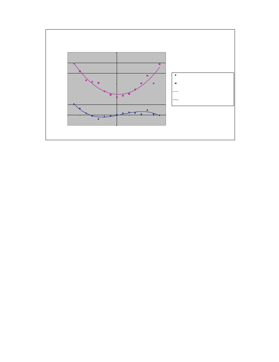
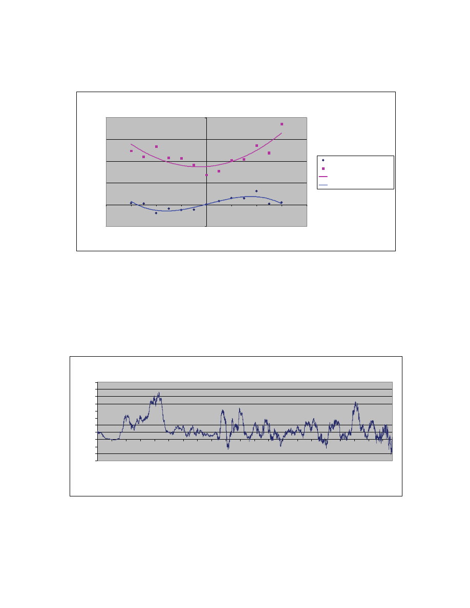
Figure 1 illustrates actual conditional returns and volatility for the DJIA dating back to

the period following the Crash of 1929. The data covers more than seven decades of

daily price changes. It clearly demonstrates that the conditional returns (average return

following prior day return of a given size) exhibit the trend reinforcing behavior for

moderate daily returns within the -2.0% to +3.5% region. This data suggests that on

average, over the long run, the market can be viewed as being in bifurcated, trend

persistent states. This nonlinear random walk or jump process, characterized by a

persistent drift toward bistable disequilibrium states (rather than the simple mean

regression) is evidenced by the positive slope of the conditional return map in the region

near the market’s long term average return.

The conditional return findings presented in Figure 1 include all data from January

1930 to January 2005 regardless of underlying economic fundamentals or liquidity issues

that affect the markets from time to time. A polynomial fit [k(R) = -159.8 R

3

+ 2.225 R

2

+ 0.1134 R - 0.0002] to the data shows an r-square of 89%. This fit suggests that the

maximum trend persistence for moderate positive returns occurs approximately after

A Bifurcation Model of Non-Stationary Markets

December 2006

10

prior returns of 2% with an average daily return on the subsequent day of slightly more

than 0.15% and the drift is toward a stable disequilibrium bull state at over +3% where

the conditional return drops to zero. Trend persistence for moderate negative returns is

greatest after prior day returns of about –1.5% and average around –0.1%. The

disequilibrium bear state is at about –2% where the trend persistence vanishes.

Bifurcation Parameter

While the empirical evidence suggests that the bi-stable disequilibrium is the main

dynamic for the capital markets’ long-term average behavior, a closer examination

reveals that at times the market is either in a single, linear equilibrium state or at the

critical bifurcation point. This situation occurred most noticeably in the era of the Great

Depression after the Crash of 1929. It has also occurred in the aftermath of the 2000

High Tech Crash.

In order to examine the market’s state transitions, we determine the slope of the

conditional return map for moderate returns around the neighborhood of zero. If the

market is in a single equilibrium state, the slope near zero should be negative (a

1

> 0)

while if bi-stable states exist, the slope near zero should be positive (a

1

< 0). To

determine a bifurcation parameter, we use a 200 day sum of the conditional returns in the

region of moderate positive prior day returns [0.025 < R(0) < 2.25%] and subtract the 200

day sum of moderate negative prior day returns [-0.025 > R(0) > -2.25%]. If the slope of

the conditional return map near zero is positive, as expected in bi-stable, trend persistent

markets, then the sum of returns after moderate positive returns should also be positive.

Moderate negative returns should be followed on average by further negative trend

persistence. Therefore a positive bifurcation parameter indicates a bi-stable market and a

A Bifurcation Model of Non-Stationary Markets

December 2006

11

negative bifurcation parameter indicates a single equilibrium state market. By using the

sum instead of the average conditional return, we also have a metric of an idealized, cost-

free, trading strategy that is long after positive prior day returns and short after negative

prior day returns.

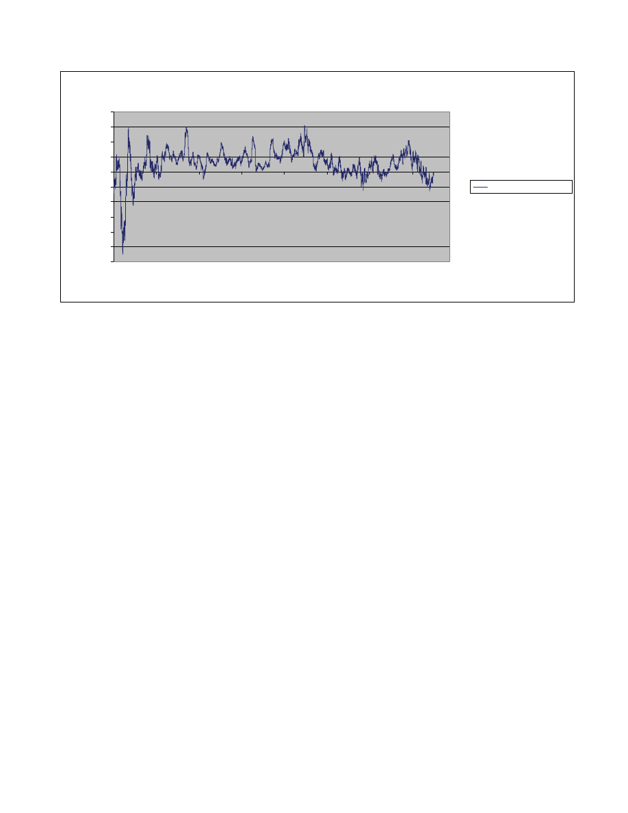
Figure 2 summarizes the bifurcation parameter for the Dow Jones Industrial Average

since 1930. The most significant periods of “single equilibrium state” occurred following

the Crash of 1929 when the market suffered from poor liquidity and disinterest on the

part of many who had been hurt as a result of the crash. Even during the 1930s there was

also a great deal of volatility in this indicator. In contrast, for many decades after the

1930s the market enjoyed strong bi-stable disequilibrium behavior. While the bifurcation

indicator fluctuated over these decades, the fluctuations were normally in positive

territory.

Dow Jones Industrial Average – Bistable Markets

Table 2 and Figure 3 present the conditional return map for the bi-stable market

periods as determined by the bifurcation parameter in Figure 2. The market was in the

bi-stable state 81.2% of the time from 1930 to 2005 and in the single equilibrium state for

only 18.8% of the time. A better resolution of the bi-stable market is achieved by

eliminating the single state and transition periods which are mean regressing rather than

trend persistent.

The conditional return findings presented in Figure 3 include all data during a

positive bifurcation parameter from January 1930 to January 2005 regardless of

underlying economic fundamentals. A polynomial fit [k(R) = -156.2 R

3

+ 2.572 R

2

+

0.145 R - 0.0003] to the data shows an r-square of 86%. This fit suggests that the peak in

A Bifurcation Model of Non-Stationary Markets

December 2006

12

trend persistence for moderate positive returns occurs approximately after prior returns of

2.5% with an average daily return on the subsequent day of slightly more than 0.25% and

the drift is toward a stable disequilibrium bull state at over +3.5% where the conditional

return drops to zero. Trend persistence for moderate negative returns is greatest after

prior day returns of about –1.5% and average around –0.1%. The disequilibrium bear

state is at about –2.5% where the trend persistence vanishes.

Dow Jones Industrial Average – Single Equilibrium and Transition Periods

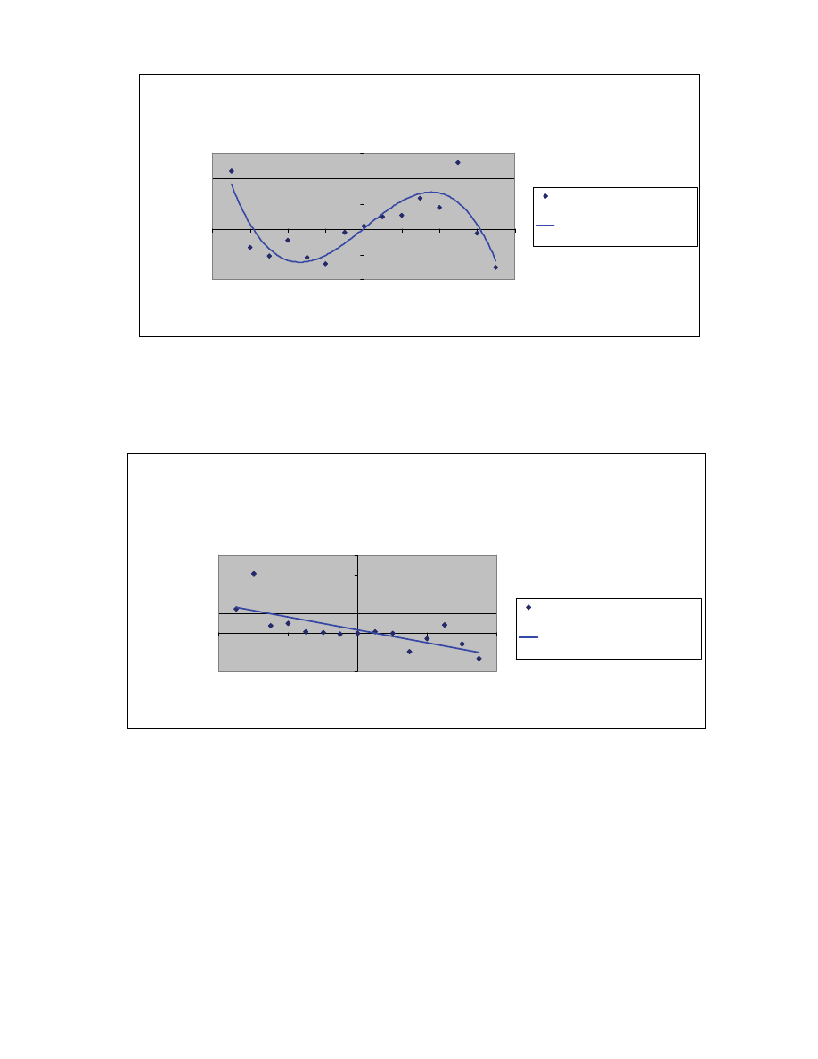
Table 3 and Figure 4 present the conditional return map for the single equilibrium

market periods. Since there is less data for the single equilibrium periods, the data is

more erratic and the null hypothesis can not be ruled out. This may be due in part to the

relatively long sample used to assess the bifurcation parameter. By the time the single

market state has been identified, often it has already transitioned to the bifurcation point

or beyond to bi-stable behavior.

The conditional return findings presented in Figure 4 include all data during a

negative bifurcation parameter from January 1930 to January 2005 regardless of

underlying economic fundamentals. A linear fit [k(R) = -0.0905 R + 0.0005] to the data

shows an r-square of 44%. However a nonlinear fit [k(R) = -119.0R

3

+ 1.116R

2

+

0.0088R + 1E-05 has a better fit with an r-square of 56%. Therefore the coefficient of

the linear term is probably between +0.0905 and -0.0088 and we conclude that the

periods when the bifurcation parameter is negative include both single state, linear state

markets and periods at the critical bifurcation state.

Business Cycle Stages

A Bifurcation Model of Non-Stationary Markets

December 2006

13

The National Bureau of Economic Research (NBER) defines periods of recession and

expansion in terms of peaks and troughs in economic activity. Periods of expansion begin

at the trough date and end at the peak date. Periods of recession begin at the peak date

and end at the trough date. DeStefano (2004) uses the peak and trough dates to separate

the business cycle into the four stages: Stage I, early expansion, begins at the trough date

and continues through one half of the expansionary period. Stage II, late expansion, is

defined as the second half of the expansionary period and concludes at the peak date.

Recessions include Stages III and IV, which, are interpreted as early decline and late

decline, respectively. Since the NBER only defines peak and trough dates, the dates that

separate Stages I and II and Stages III and IV occur in the chronological middle of the

trough-to-peak and peak-to-trough time periods.

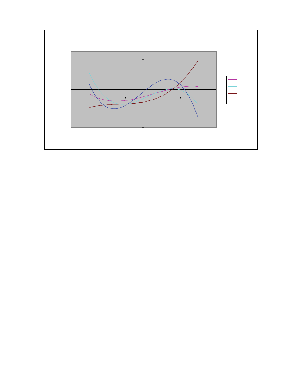
In order to assess how business cycle phases affect market equilibrium states, we

examine the DJIA conditional returns and volatility during the four business cycle phases

as defined by DeStefano (2004). Table 4 summarizes the best data fit for the periods

defined by DeStefano as Stages I, II, III and IV as well as for combined Stage I and II

(expansion) and combined Stage III and IV (recession). Figure 5 illustrates the

conditional return maps for each of the four business cycle stages. The results show that

the expansionary phases of the business cycle have well defined bistable market behavior

with trend persistence after moderate returns and mean regressing dynamics after large

returns in either direction.

Volume Based Bifurcation

Table 5 and Figure 6 present the conditional return map for market periods following

prior day volume increases of 25% or more. The conditional return findings include all

A Bifurcation Model of Non-Stationary Markets

December 2006

14

data following rising volume from January 1930 to January 2005 regardless of underlying

economic fundamentals. A polynomial fit [k(R) = -151.4 R

3

+ 1.22 R

2

+ 0.156 R -

0.00003] to the data shows an r-square of 78%. This fit suggests that the peak in trend

persistence for moderate positive returns occurs approximately after prior returns of 2.5%

with an average daily return on the subsequent day of slightly more than 0.25% and the

drift is toward a stable disequilibrium bull state at over +3.0% where the conditional

return drops to zero. Trend persistence for moderate negative returns is greatest after

prior day returns of about –1.5% and average around –0.25%. The disequilibrium bear

state is at about –3.0% where the trend persistence vanishes.

Table 6 and Figure 7 present the conditional return map for periods following a 25%

or greater decline in volume. The conditional return findings are based on all data

following a daily 25% volume decline from January 1930 to January 2005 regardless of

underlying economic fundamentals. The conditional return map in this case resembles

the single equilibrium, mean regressive market periods. A linear fit [k(R) = -0.329 R +

0.0015] to the data shows an r-square of 53%.

10 Year US Treasury Bonds

Interest rates also show significant nonlinear trend persistence and bi-stable or

bifurcated states. Table 7 and Figure 8 present the conditional return map and volatility

of returns for the 10 Year US Treasury Bond from 1962 to 2003. Interest rate change

persistence follows the same pattern of increasing volatility with the magnitude of prior

day rate changes. A polynomial fit for conditional interest rate changes [-174.0 R

3

+

0.459 R

2

+ 0.148 R] shows an r-square of 0.77 while volatility of rate changes has a best

fit [7.16 R

2

+0.042 R + 0.0087] with an r-square of 0.70. Moderate positive rate

A Bifurcation Model of Non-Stationary Markets

December 2006

15

increases on the prior day are followed on average by further rate increases and moderate

interest rate declines are followed on average by further interest rate declines. Rising rate

persistence appears to extend out to +3% where it stabilizes at zero. Declining rate

persistence tends to achieve stability in the –3% region. Therefore the bond market

information dissemination process can also be characterized as a drift towards bistable

disequilibrium.

A bifurcation parameter can also be calculated for the US Treasury Bond and is

shown in Figure 9. For the period shown, the bifurcation parameter has been positive

91% of the time, corresponding to a bistable equilibrium market. However, the periods

for which this bifurcation parameter is negative do not show a statistically significant

deviation from the bistable pattern. This suggests that by the time the bifurcation

parameter has detected a single equilibrium state, the market has already bifurcated back

to the normal bistable states.

SUMMARY AND CONCLUSIONS

Empirical evidence suggests that most of the time both the stock and bond markets are

trend persistent (rather than mean regressing) drifting toward either a bull state

equilibrium rate of return or a bear state equilibrium. The relative stability of Bull and

Bear equilibrium states vary with the business cycle.

The non-stationary characteristic of market states has significant implications for

traders. Trading rules can be based on the trend persistent nature of conditional returns.

However, since the market process is non-stationary, an adaptive strategy is necessary

that can switch from trend persistent trading rules to mean regressing rules as the market

undergoes state transitions. Late stage periods of economic contraction appear to be least

A Bifurcation Model of Non-Stationary Markets

December 2006

16

efficient having the highest degree of trend persistence after moderate returns; early

stage periods of economic contraction have the greatest degree of trend persistence

following large returns.

Volume has also been shown to be a useful indicator of trend persistent markets.

Conditional returns following rising volume tend to exhibit above average trend

persistence. Therefore markets can be viewed as restructuring their information structure

in response to the volume of information arriving at any point in time.

The post Crash of 1929 and Crash of 2000 periods suggest that the bi-stable

disequilibrium markets can lead to extremes in valuation, resulting in instability and

structural changes in the aftermath of a crash. The empirical evidence suggests that

while bi-stable markets may often be self-correcting, at times the trend persistence may

result in valuation extremes. In response, it appears that the market undergoes

restructuring by switching to more stable, mean regressing rather then trend persistent

behavior.

REFERENCES

Beja, A., and M. B. Goldman. (1980). “On the Dynamic Behavior of Prices in
Disequilibrium.” Journal of Finance (May 1980): 235—47.

Beja, A., and N. H. Hakansson. (1977). “Dynamic Market Processes and Rewards to Up-
to-Date Information.” Journal of Finance (May 1977): 291 —304.

Black, S. V. (1976). “Rational Response to Shocks in a Dynamic Model of Capital Asset
Prices.” American Economic Review (December 1976): 767—79.

Boulding, K. E. (1981a). Ecodynamics: A New Theory of Societal Evolution. Beverly
Hills: Sage Publications, 1981.

Boulding, K.E. (1981b) Evolutionary Economics. Beverly Hills: Sage Publications. 1981.

Callen, E., and Shapero, D. (1974), "A Theory of Social Imitation," Physics Today, July,
1974.

A Bifurcation Model of Non-Stationary Markets

December 2006

17

Chauvet, Marcelle (1998a). "An Econometric Characterization of Business Cycle
Dynamics with Factor Structure and Regime Switching," International Economic Review,
1998, v39 (4, Nov), 969-996.

Chauvet, Marcelle (1998b). "Stock Market Fluctuations and the Business Cycle," Journal
of Economic and Social Measurement, 1998, v25 (3/4), 235-257.

Chauvet, Marcelle and Simon Potter (2000). "Coincident And Leading Indicators of the
Stock Market," Journal of Empirical Finance, 2000, v7 (1, May), 87-111.

Chauvet, Marcelle and Simon Potter (2001). “Nonlinear Risk,” Macroeconomic
Dynamics, Vol. 5, No. 4, (September 2001): 621-46.

Clark, P. B. (1973). “A Subordinated Stochastic Process Model with Finite Variance for
Security Prices.” Econometrica (January 1973): 135—55.

Cohen, K. J.: U. A. Hawawini; S. F. Maier; R. A. Schwarz; and D. K. Whitcomb (1980).
“Implications of Microstructure Theory for Empirical Research on Stock Price
Behavior.” Journal of Finance, (May 1980): 249—57.

Copeland, T. E. (1976) “A Model of Asset Trading Under the Assumption of Sequential
Information Arrival.” Journal of Finance (September 1976): 1149—68.

Cozzolino, J. M., and M.J. Zahner (1973). “The Maximum-Entropy Distribution of the
Future Market Price of a Stock.” Operations Research (1973): 1200—11.

DeStefano, M. (2004), “Stock Returns and the Business Cycle.” The Financial Review
Vol.39, No.4, November 2004, 527-547.

Dopfer, K., The Evolutionary Foundations of Economics, Cambridge University Press,
(2005).

Fama, Eugene F. (1970). “Efficient Capital Markets: A Review of Theory and Empirical
Work.” Journal of Finance (May 1970): 383 —417.

Fama, Eugene F. and Kenneth R. French (1989). "Business Conditions and Expected
Returns on Stocks and Bonds," Journal of Financial Economics, 1989, v25 (1), 23-50.

Georgescu-Roegen, N. (1971), Entropy Law and Economic Processes. Boston: Harvard
University Press, 1971.

Grossman, S. and J. Stiglitz (1976). “Information and Competitive Price Systems.”
American Economic Review (May 1976): 246—53.

A Bifurcation Model of Non-Stationary Markets

December 2006

18

Groth, J. (1979). “Security-Relative Information Market Efficiency: Some Empirical
Evidence.” Journal of Financial and Quantitative Analysis (September l979): 573—93.

Guidolin, Massimo and Allan Timmermann (2005). “An Econometric Model of
Nonlinear Dynamics in the Joint Distribution of Stock and Bond Returns.” Forthcoming
in Journal of Applied Econometrics. 2005.

Haken, H. (1975). “Cooperative Phenomena in Systems Far From Thermal Equilibrium
and in Nonphysical Systems.” Review of Modern Physics, Vol. 47, No. 1 (January 1975):
68-119.

Hong, H., and Stein, J., “A unified theory of underreaction, momentum trading and
overreaction in asset markets”, Journal of Financial Economics, 41, 401 (1999)

Majthay, A. (1980). “Bifurcations in Dynamical Systems.” Decision Sciences (April
1980): 384—407.

Morse, D. (1980), “Asymmetrical Information in Securities Markets and Trading
Volume.” Journal of Financial and Quantitative Analysis (December 1980): 1129—48.

Murphy, R. (1965). Adaptive Processes in Economic Systems. Academic Press, 1965.

Nawrocki, David (1984). "Entropy, Bifurcation, And Dynamic Market Disequilibrium,"
Financial Review, 1984, v19 (2), 266-284.

Nawrocki, David N. (1995). "Expectations, Technological Change, Information and the
Theory of Financial Markets," International Review of Financial Analysis, 1995, v4
(2/3), 85-105.

Nawrocki, David N. (1996) "Market Dependence and Economic Events," Financial
Review, 1996, v31 (2, May), 287-312.

Nicolis, G., and I. Prigogine (1977). Self-Organization in Nonequilibrium Systems. John
Wiley and Sons, 1977.

Oldfield, G.; R. Rogalski; and R. Jarrow (1977). “An Autoregressive Jump Process for
Common Stock Returns.” Journal of Financial Economics (December 1977): 389—418.

Perez-Quiros, Gabriel and Allan Timmermann. "Firm Size and Cyclical Variations in
Stock Returns," Journal of Finance, 2000, v55 (3, Jun), 1229-1262.

Perez-Quiros, Gabriel and Allan Timmermann. "Business Cycle Asymmetries In Stock
Returns: Evidence from Higher Order Moments and Conditional Densities," Journal of
Econometrics, 2001, v103 (1-2, Jul), 259-306.

A Bifurcation Model of Non-Stationary Markets

December 2006

19

Philippatos, G., and N. Gressis (1975). “Conditions of Equivalence among EV, SSD and
EH Portfolio Selection Criteria: The Case for Uniform Normal and Lognormal
Distributions.” Management Science (February 1975): 617—25.

Philippatos, G., and C. Wilson (1972), “Entropy, Market Risk, and the Selection of
Efficient Portfolios.” Applied Economics (September 1972): 209—20.

Shiller, R. J., Irrational Exuberance, Princeton University Press (2000)

Schliefer, A., Inefficient Markets, An Introduction to Behavioral Finance, Oxford
University Press, (2000)

Thom, R. (1972), Structural Stability and Morphogenesis. Benjamin-Addison Wesley.
1972.

Vaga, Tonis. (1990). “The Coherent Market Hypothesis.” Financial Analysts Journal,
Vol. 46 (6), 36-49.

Weidlich, W. (1971), "The Statistical Description of Polarization Phenomena in
Society," British Journal of Mathematical and Statistical Psychology, 24, 1971.

Weidlich, W., and Haag, G. (1983), Concepts and Methods of a Quantitative Sociology,
Springer-Verlag, New York, 1983.

Whitelaw, Robert F. (1994). "Time Variations and Covariations in the Expectation and
Volatility of Stock Market Returns," Journal of Finance, 1994, v49 (2), 515-541.

Wyart, M., and Bouchaud, J. P., “Self-referential behavior, overreaction and conventions
in financial markets”, arXiv:cond-mat/0303584 v2 23 June 2003.

A Bifurcation Model of Non-Stationary Markets

December 2006

20

Conditional
Return

0.05% -0.23% 0.53% 0.32% 0.09% -0.05% -0.19% -0.08% -0.04% 0.03%

Standard
Deviation

4.13% 2.21% 2.46% 2.09% 1.67% 1.59% 1.54% 1.14% 0.97% 0.86%

Relative
Frequency

0.47% 0.21% 0.26% 0.50% 0.86% 1.64% 3.74% 8.46% 17.83% 28.20%

Prior Day
Return

R<-
4.25%

-4.00% -3.50% -3.00% -2.50% -2.00% -1.50% -1.00% -0.50% 0.00%

T-Test (p
of Null)

95.10% 46.31% 16.22% 17.69% 62.48% 37.36% 0.02% 0.02% 0.02% 99.40%

Conditional
Return

0.09% 0.13% 0.10% 0.05% 0.24% 0.04% -0.01% 0.18% -0.31% 0.30% -0.08%

Standard
Deviation

0.93% 1.02% 1.22% 1.52% 1.88% 1.52% 2.43% 1.82% 2.30% 2.79% 3.18%

Relative
Frequency

20.30% 9.68% 3.92% 1.71% 0.91% 0.37% 0.33% 0.18% 0.12% 0.10% 0.21%

Prior Day
Return

0.50% 1.00% 1.50% 2.00% 2.50% 3.00% 3.50% 4.00% 4.50% 5.00% R>5.25%

T-Test (p
of Null)

0.01% 0.00% 11.82% 79.42% 13.99% 92.08% 90.69% 62.26% 50.68% 68.04% 84.09%

Table 1. Dow Jones Industrial Average Conditional Returns and Volatility

(2-Jan-1930 to 13-Jan-05)

Conditional
Return

-0.24% 0.13% 0.42% 0.24% 0.09% -0.15% -0.28% -0.11% -0.05% 0.02%

Standard
Deviation

4.62% 1.75% 1.94% 1.76% 1.66% 1.47% 1.39% 1.10% 0.90% 0.81%

Relative
Frequency

0.23% 0.11% 0.14% 0.29% 0.64% 1.16% 2.84% 6.71% 14.57% 23.27%

Prior Day
Return

R<-
4.25%

-4.00% -3.50% -3.00% -2.50% -2.00% -1.50% -1.00% -0.50% 0.00%

T-Test (p
of Null)

70.52% 77.93% 30.38% 36.68% 66.59% 8.44% 0.00% 0.00% 0.01% 88.96%

Conditional
Return

0.10% 0.15% 0.11% 0.26% 0.16% 0.31% 0.11% 0.50% 0.48% 0.53% 0.07%

Standard
Deviation

0.82% 0.96% 1.03% 1.26% 1.23% 1.39% 1.77% 1.53% 1.41% 1.74% 3.69%

Relative
Frequency

16.49% 7.86% 2.92% 1.18% 0.59% 0.26% 0.21% 0.11% 0.06% 0.05% 0.06%

Prior Day
Return

0.50% 1.00% 1.50% 2.00% 2.50% 3.00% 3.50% 4.00% 4.50% 5.00% R>5.25%

T-Test (p
of Null)

0.00% 0.00% 6.57% 0.69% 27.01% 16.80% 76.24% 16.94% 28.62% 38.66% 97.11%

Table 2. Bistable State DJIA Conditional Returns and Volatility

(2-Jan-1930 to 13-Jan-05)

A Bifurcation Model of Non-Stationary Markets

December 2006

21

Conditional
Return

0.34% -0.64% 0.66% 0.42% 0.09% 0.17% 0.08% 0.01% -0.01% 0.04%

Standard
Deviation

3.62% 2.63% 3.03% 2.49% 1.71% 1.82% 1.91% 1.30% 1.26% 1.06%

Relative
Frequency

0.24% 0.10% 0.12% 0.21% 0.22% 0.48% 0.90% 1.75% 3.26% 4.92%

Prior Day
Return

R<-
4.25%

-4.00% -3.50% -3.00% -2.50% -2.00% -1.50% -1.00% -0.50% 0.00%

T-Test (p
of Null)

56.45% 28.41% 33.91% 32.13% 82.00% 46.04% 72.00% 80.91% 44.21% 77.53%

Conditional
Return

0.05% 0.04% 0.07% -0.42% 0.40% -0.56% -0.21% -0.37% -1.25% 0.02% -0.14%

Standard
Deviation

1.27% 1.24% 1.66% 1.91% 2.72% 1.64% 3.27% 2.21% 2.85% 3.86% 3.01%

Relative
Frequency

3.81% 1.81% 1.00% 0.53% 0.31% 0.11% 0.13% 0.06% 0.05% 0.04% 0.15%

Prior Day
Return

0.50% 1.00% 1.50% 2.00% 2.50% 3.00% 3.50% 4.00% 4.50% 5.00% R>5.25%

T-Test (p
of Null)

65.88% 87.95% 74.16% 2.28% 29.67% 11.53% 72.78% 54.49% 18.92% 99.69% 77.80%

Table 3. Linear State DJIA Conditional Returns and Volatility

(2-Jan-1930 to 13-Jan-05)

Stage I

= -111.1R

3

+ 1.91R

2

+ 0.132R + 0.0001

Stage II

= -403.6R

3

+ 2.85R

2

+ 0.219R - 0.0004

Stage III

= 18.79R

3

+ 6.57R

2

+ 0.136R - 0.0015

Stage IV

= -607.2R

3

- 2.77R

2

+ 0.393R + 0.0014

Stages I&II

= -293.4R

3

+ 2.56R

2

+ 0.184R - 0.0002

Stages III&IV

= 53.6R

3

+ 1.63R

2

+ 0.0889R - 9E-05

All DJIA

= -159.8 R

3

+ 2.225 R

2

+ 0.1134 R - 0.0002

Bistable

= -156.2 R

3

+ 2.572 R

2

+ 0.145 R - 0.0003

Linear

= -0.0905 R + 0.0005

Transition

= -119.0R

3

+ 1.116R

2

+ 0.0088R + 1E-05

k(R) = -a

3

R

3

-a

2

R

2

-a

1

R -a

0

Table 4. DJIA Conditional Return Map Best Fits for DeStephano (2004) Business

Cycle Stages (1948 - 2001)

A Bifurcation Model of Non-Stationary Markets

December 2006

22

Conditional
Return

0.32% -0.03% 0.40% -0.19% -0.16% -0.10% -0.22% -0.29% -0.05% 0.02%

Standard
Deviation

4.51% 2.09% 2.67% 1.49% 1.82% 1.23% 1.21% 1.16% 0.99% 1.02%

Relative
Frequency

0.25% 0.11% 0.12% 0.22% 0.35% 0.43% 0.68% 0.81% 0.97% 1.15%

Prior Day
Return

R < -
4.25%

-4.00% -3.50% -3.00% -2.50% -2.00% -1.50% -1.00% -0.50% 0.00%

T-Test (p
of Null)

65.10% 89.92% 51.81% 35.14% 42.28% 35.69% 2.18% 0.09% 32.44% 96.71%

Conditional
Return

0.10% 0.11% 0.24% 0.15% 0.52% -0.03% -0.39% 0.26% -0.40%

Standard
Deviation

0.97% 0.90% 1.02% 1.12% 2.28% 1.49% 1.53% 1.76% 2.33%

Relative
Frequency

1.88% 1.91% 1.22% 0.60% 0.40% 0.15% 0.14% 0.12% 0.23%

Prior Day
Return

0.50% 1.00% 1.50% 2.00% 2.50% 3.00% 3.50% 4.00% R>4.25%

T-Test (p
of Null)

17.47% 7.98% 0.16% 23.29% 6.23% 85.22% 17.02% 53.20% 22.89%

Table 5. Bistable State DJIA Conditional Returns and Volatility

After >+25% Prior Day Volume Increase (2-Jan-1930 to 13-Jan-05)

Conditional
Return

0.34% -0.64% 0.66% 0.42% 0.09% 0.17% 0.08% 0.01% -0.01% 0.04%

Standard
Deviation

3.62% 2.63% 3.03% 2.49% 1.71% 1.82% 1.91% 1.30% 1.26% 1.06%

Relative
Frequency

0.24% 0.10% 0.12% 0.21% 0.22% 0.48% 0.90% 1.75% 3.26% 4.92%

Prior Day
Return

R<-
4.25%

-4.00% -3.50% -3.00% -2.50% -2.00% -1.50% -1.00% -0.50% 0.00%

T-Test (p
of Null)

56.45% 28.41% 33.91% 32.13% 82.00% 46.04% 72.00% 80.91% 44.21% 77.53%

Conditional
Return

0.05% 0.04% 0.07% -0.42% 0.40% -0.56% -0.21% -0.37% -1.25% 0.02% -0.14%

Standard
Deviation

1.27% 1.24% 1.66% 1.91% 2.72% 1.64% 3.27% 2.21% 2.85% 3.86% 3.01%

Relative
Frequency

3.81% 1.81% 1.00% 0.53% 0.31% 0.11% 0.13% 0.06% 0.05% 0.04% 0.15%

Prior Day
Return

0.50% 1.00% 1.50% 2.00% 2.50% 3.00% 3.50% 4.00% 4.50% 5.00% R>5.25%

T-Test (p
of Null)

65.88% 87.95% 74.16% 2.28% 29.67% 11.53% 72.78% 54.49% 18.92% 99.69% 77.80%

Table 6. Linear State DJIA Conditional Returns and Volatility

After >=25% Prior Day Volume Decline (2-Jan-1930 to 13-Jan-05)

A Bifurcation Model of Non-Stationary Markets

December 2006

23

Conditional
Return

-0.10% 0.09% 0.04% 0.03% -0.19% -0.09% -0.12% -0.11% 0.01%

Standard
Deviation

1.72% 1.49% 1.24% 1.10% 1.33% 1.08% 1.06% 0.91% 0.68%

Relative
Frequency

0.16% 0.17% 0.25% 0.79% 1.43% 3.54% 7.77% 17.73% 36.28%

Prior Day
Return

-4.00% -3.50% -3.00% -2.50% -2.00% -1.50% -1.00% -0.50% 0.00%

T-Test (p
of Null)

81.17% 81.32% 89.91% 85.55% 7.31% 10.73% 0.13% 0.00% 91.04%

Conditional
Return

0.09% 0.15% 0.14% 0.31% 0.02% 0.05% 0.26% 0.18%

Standard
Deviation

0.77% 1.02% 1.04% 1.35% 1.19% 1.85% 1.85% 1.47%

Relative
Frequency

17.89% 7.66% 3.20% 1.51% 0.80% 0.36% 0.18% 0.25%

Prior Day
Return

0.50% 1.00% 1.50% 2.00% 2.50% 3.00% 3.50% 4.00%

T-Test (p
of Null)

0.00% 0.01% 1.83% 0.57% 89.65% 88.39% 55.94% 55.20%

Table 7. 10 Year US Treasury Conditional Returns and Volatility (1-Feb-1963 to
29-Apr-04)

A Bifurcation Model of Non-Stationary Markets

December 2006

24

Figure 1. Historical Conditional Returns and Volatility for the Dow Jones

Industrial Average

Historical Conditional Returns and Volatility

(Dow Jones Industrial Average: 1930 - 2005)

Volatility = 11.37R

2

- 0.0294R + 0.0099

r

2

= 0.898

k(R) = -159.8R

3

+ 2.224R

2

+ 0.1134R - 0.0002

r

2

= 0.89

-0.5%

0.0%

0.5%

1.0%

1.5%

2.0%

2.5%

3.0%

-4.0%

-3.0%

-2.0%

-1.0%

0.0%

1.0%

2.0%

3.0%

4.0%

Prior Day Return R(0)

A

ver

ag

e

N

ext

D

ay

R

et

u

rn

R

(t

) an

d

V

o

la

ti

lit

y

Dow Jones Industrials Conditional Returns
(1930 - 2005)
Volatility of Return

Poly. (Volatility of Return)

Poly. (Dow Jones Industrials Conditional
Returns (1930 - 2005))

A Bifurcation Model of Non-Stationary Markets

December 2006

25

Figure 2. Dow Jones Industrial Average Bifurcation Parameter

Bifurcation Parameter Dow Jones Industrial Average

-120%

-100%

-80%

-60%

-40%

-20%

0%

20%

40%

60%

80%

Jan-30

Dec-39

Dec-49

Dec-59

Dec-69

Dec-79

Dec-89

Dec-99

Time

B

if

u

rcat

io

n

P

ar

am

et

er

Bifurcation Parameter

A Bifurcation Model of Non-Stationary Markets

December 2006

26

Figure 3. Bi-stable Market Conditional Returns and Volatility

Single State Markets: Conditional Returns and Volatility

(Dow Jones Industrial Average: 1930 - 2005)

k(R) = -0.0905R + 0.0005

r

2

= 0.44

Volatility = 14.00R

2

+ 0.0086R + 0.0123

r

2

= 0.76

-1.0%

-0.5%

0.0%

0.5%

1.0%

1.5%

2.0%

2.5%

3.0%

3.5%

-4.0%

-3.0%

-2.0%

-1.0%

0.0%

1.0%

2.0%

3.0%

4.0%

Prior Day Return R(0)

A

ve

ra

g

e

N

e

xt

D

a

y R

et

u

rn

R

(t

) an

d

V

o

la

tilit

y

Dow Jones Industrials Conditional Returns
(1930 - 2005)
Volatility of Return

Linear (Dow Jones Industrials Conditional
Returns (1930 - 2005))
Poly. (Volatility of Return)

Bistable Markets: Conditional Returns and Volatility

(Dow Jones Industrial Average: 1930 - 2005)

k(R) = -156.2R

3

+ 2.572R

2

+ 0.145R - 0.0003

r

2

= 0.86

Volatility = 7.709R

2

- 0.056R + 0.0094

r

2

= 0.92

-0.5%

0.0%

0.5%

1.0%

1.5%

2.0%

2.5%

-4.0%

-3.0%

-2.0%

-1.0%

0.0%

1.0%

2.0%

3.0%

4.0%

Prior Day Return R(0)

A

ver

ag

e N

ext

D

ay R

et

u

rn

R

(t

) a

n

d

V

o

la

tili

ty

Dow Jones Industrials Conditional Returns
(1930 - 2005)
Volatility of Return

Poly. (Dow Jones Industrials Conditional
Returns (1930 - 2005))
Poly. (Volatility of Return)

A Bifurcation Model of Non-Stationary Markets

December 2006

27

Figure 4. Single Equilibrium Market Conditional Returns and Volatility

A Bifurcation Model of Non-Stationary Markets

December 2006

28

Figure 5. Business Cycle Stages I-IV DJIA Conditional Returns and Volatility

DJIA Conditional Returns During Business Cycle Stages

-0.8%

-0.6%

-0.4%

-0.2%

0.0%

0.2%

0.4%

0.6%

0.8%

1.0%

1.2%

-4.0%

-3.0%

-2.0%

-1.0%

0.0%

1.0%

2.0%

3.0%

4.0%

Prior Day Return, R(0)

C

o

n

d

it

io

n

al R

et

u

rn

Stage I
Stage II
Stage III
Stage IV

A Bifurcation Model of Non-Stationary Markets

December 2006

29

Figure 6. Conditional Returns Following Rising Volume Exhibit Bistable, Trend

Persistent Behavior

Figure 7. Conditional Returns Following Declining Volume Exhibit Single State,

Mean Regressive Behavior

Dow Jones Industrial Average

(Returns After 25% Volume Increase)

k(R) = -151.38R

3

+ 1.2187R

2

+ 0.1558R - 3E-05

r

2

= 0.78

-0.40%

-0.20%

0.00%

0.20%

0.40%

0.60%

-4%

-3%

-2%

-1%

0%

1%

2%

3%

4%

Prior Day Return, R(0)

N

e

x

t Da

y

Re

tu

rn

, R(

t)

Conditional Returns on Rising
Volume
Poly. (Conditional Returns on
Rising Volume)

Dow Jones Industrial Average

(Returns After 25% Volume Decline)

k(R) = -0.329R + 0.0015

r

2

= 0.53

-2.0%

-1.0%

0.0%

1.0%

2.0%

3.0%

4.0%

-4%

-2%

0%

2%

4%

Prior Day Return, R(0)

Next Da

y

Return, R(t)

Conditional Returns on Declining
Volume
Linear (Conditional Returns on
Declining Volume)

A Bifurcation Model of Non-Stationary Markets

December 2006

30

Figure 8. 10 Year US Treasury Bond Market Conditional Returns and Volatility

Figure 9. 10 Year US Treasury Bond Bifurcation Parameter

10 Year Treasury Bifurcation Parameter

-30%

-20%

-10%

0%

10%

20%

30%

40%

50%

60%

70%

80%

Ja

n

-63

Ja

n

-65

Ja

n

-67

Ja

n

-69

Ja

n

-71

Ja

n

-73

Ja

n

-75

Ja

n

-77

Ja

n

-79

Ja

n

-81

Ja

n

-83

Ja

n

-85

Ja

n

-87

Ja

n

-89

Ja

n

-91

Ja

n

-93

Ja

n

-95

Ja

n

-97

Ja

n

-99

Ja

n

-01

Ja

n

-03

10 Year US Treasury Bonds (1962 - 2003)

Volatility = 7.16R

2

+ 0.0422R + 0.0087

r

2

= 0.70

k(R) = -174.0R

3

+ 0.459R

2

+ 0.1475R + 8E-05

r

2

= 0.77

-0.5%

0.0%

0.5%

1.0%

1.5%

2.0%

-4.0%

-3.0%

-2.0%

-1.0%

0.0%

1.0%

2.0%

3.0%

4.0%

Prior Day Rate Change (R)

C

o

n

d

itio

n

a

l R

a

te

C

h

a

n

g

e

a

n

d

V

o

la

tility

Conditional Returns
Volatility
Poly. (Volatility)
Poly. (Conditional Returns)