5

Manifolds

Intuitively, a manifold is a generalization of curves and surfaces to arbitrary dimen-
sion. While there are many different kinds of manifolds—topological manifolds,
C

k

-manifolds, analytic manifolds, and complex manifolds, in this book we are con-

cerned mainly with smooth manifolds.

5.1 Topological Manifolds

We first recall a few definitions from point-set topology. For more details, see Ap-
pendix A. A topological space is second countable if it has a countable basis. A
neighborhood of a point p in a topological space M is any open set containing p. An
open cover of M is a collection

{U

α

}

α

∈A

of open sets in M whose union

%

α

∈A

U

α

is M.

Definition 5.1. A topological space M is locally Euclidean of dimension n if every
point p in M has a neighborhood U such that there is a homeomorphism φ from U
onto an open subset of

R

n

. We call the pair (U, φ

: U −

→ R

n

)

a chart, U a coordinate

neighborhood or a coordinate open set, and φ a coordinate map or a coordinate
system on U . We say that a chart (U, φ) is centered at p

∈ U if φ(p) = 0. A chart

(U, φ) about p

simply means that (U, φ) is a chart and p

∈ U.

Definition 5.2. A topological manifold of dimension n is a Hausdorff, second count-
able, locally Euclidean space of dimension n.

For the dimension to be well defined, we need to know that for n

= m an open

subset of

R

n

is not homeomorphic to an open subset of

R

m

. This is indeed true, but is

not easy to prove (see [4] for a discussion and further references). We will not pursue
this point as we are mainly interested in smooth manifolds, for which the analogous
result is easy to prove (Corollary 8.8). Of course, if a topological manifold has
several connected components, it is possible for each component to have a different
dimension.

48

5 Manifolds

Example 5.3. The Euclidean space

R

n

is covered by a single chart (

R

n

,

1

R

n

)

, where

1

R

n

: R

n

−

→ R

n

is the identity map. It is the prime example of a topological manifold.

Every open subset of

R

n

is also a topological manifold, with chart (U, 1

U

)

.

Recall that the Hausdorff condition and second countability are “hereditary prop-

erties’’; that is, they are inherited by subspaces: a subspace of a Hausdorff space is
Hausdorff (Proposition A.23) and a subspace of a second countable space is second
countable (Proposition A.19). So any subspace of

R

n

is automatically Hausdorff and

second countable.

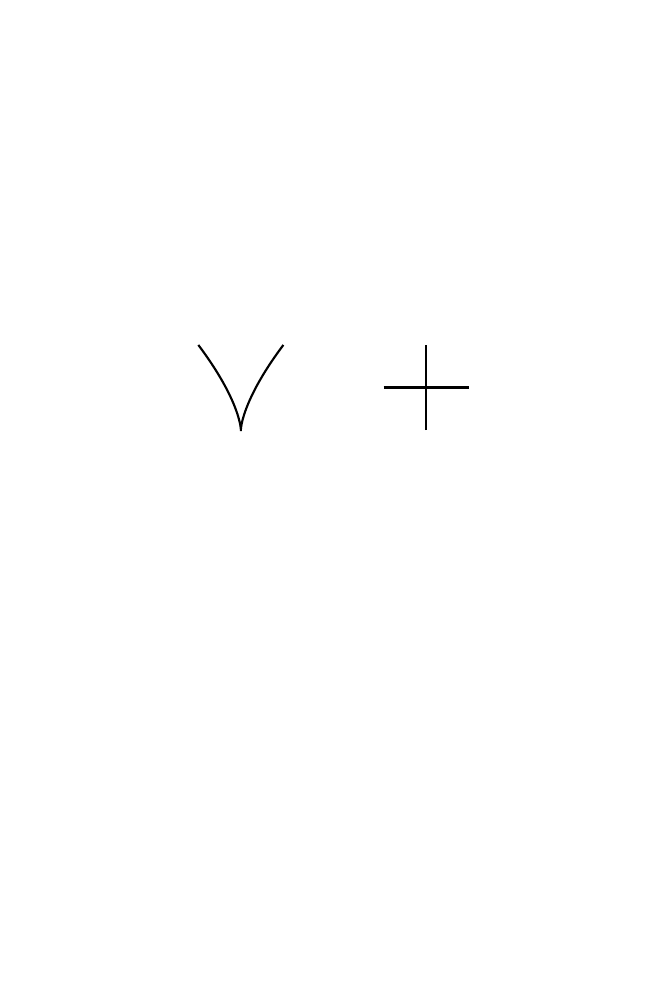
Example 5.4 (The cusp). The graph of y

= x

2/3

in

R

2

is a topological manifold

(Figure 5.1(a)). By virtue of being a subspace of

R

2

, it is Hausdorff and second

countable. It is locally Euclidean, because it is homeomorphic to

R via (x, x

2/3

)

→ x.

(a) Cusp

(b) Cross

Fig. 5.1.

Example 5.5 (The cross). Show that the cross in

R

2

in Figure 5.1 with the subspace

topology is not locally Euclidean at p, and so cannot be a topological manifold.

Solution. If a space is locally Euclidean of dimension n at p, then p has a neighbor-
hood U homeomorphic to an open ball B

:= B(0, ) ⊂ R

n

with p mapping to 0.

The homeomorphism

: U −

→ B restricts to a homeomorphism: U − {p} −

→ B − {0}.

Now B

− {0} is either connected if n ≥ 2 or has two connected components if n = 1.

Since U

−{p} has four connected components, there can be no homeomorphism from

U

− {p} to B − {0}. This contradiction proves that the cross is not locally Euclidean

at p.

5.2 Compatible Charts

Definition 5.6. Two charts (U, φ

: U −

→ R

n

)

, (V , ψ

: V −

→ R

n

)

of a topological

manifold are C

∞

-compatible if the two maps

φ

◦

ψ

−1

: ψ(U ∩ V ) −

→ φ(U ∩ V ), ψ

◦

φ

−1

: φ(U ∩ V ) −

→ ψ(U ∩ V )

are C

∞

(Figure 5.2). These two maps are called the transition functions between the

charts. If U

∩ V is empty, then the two charts are automatically C

∞

-compatible.

To simplify the notation, we will sometimes write U

αβ

for U

α

∩ U

β

and U

αβγ

for

U

α

∩ U

β

∩ U

γ

.

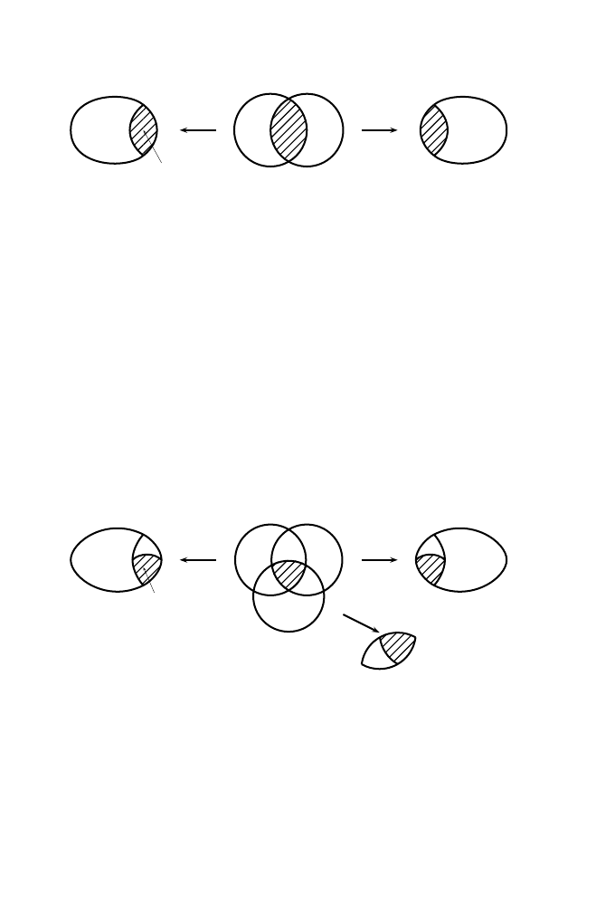
5.2 Compatible Charts

49

φ

ψ

U

V

φ (U

∩ V )

Fig. 5.2. The transition function ψ

◦

φ

−1

is defined on φ(U

∩ V ).

Since we are interested only in C

∞

-compatible charts, we often omit to mention

C

∞

and speak simply of compatible charts.

Definition 5.7. A C

∞

atlas or simply an atlas on a locally Euclidean space M is a

collection

{(U

α

, φ

α

)

} of C

∞

-compatible charts that cover M, i.e., such that M

=

%

α

U

α

.

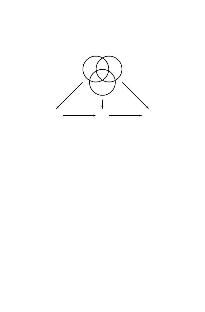
Although the C

∞

compatibility of charts is clearly reflexive and symmetric, it

is not transitive. The reason is as follows. Suppose (U

1

, φ

1

)

is C

∞

-compatible

with (U

2

, φ

2

)

, and (U

2

, φ

2

)

is C

∞

-compatible with (U

3

, φ

3

)

. Note that the three

coordinate functions are simultaneously defined only on the triple intersection U

123

.

Thus, the composite

φ

3 ◦

φ

−1

1

= (φ

3 ◦

φ

−1

2

)

◦

(φ

2 ◦

φ

−1

1

)

is C

∞

but only on φ

1

(U

123

)

, not necessarily on φ

1

(U

13

)

(Figure 5.3). A priori we

know nothing about φ

3 ◦

φ

−1

1

on φ

1

(U

13

− U

123

)

and so we cannot conclude that

(U

1

, φ

1

)

and (U

3

, φ

3

)

are C

∞

-compatible.

φ

1

(U

123

)

φ

1

φ

2

φ

3

U

1

U

2

U

3

Fig. 5.3. φ

3 ◦

φ

−1

1

is C

∞

on φ

1

(U

123

)

.

We say that a chart (V , ψ) is compatible with an atlas

{(U

α

, φ

α

)

} if it is compatible

with all the charts (U

α

, φ

α

)

of the atlas.

Lemma 5.8. Let

{(U

α

, φ

α

)

} be an atlas on a locally Euclidean space. If two charts

(V , ψ ) and (W, σ ) are both compatible with the atlas

{(U

α

, φ

α

)

}, then they are

compatible with each other.

50

5 Manifolds

Proof. (See Figure 5.4.) Let p

∈ V ∩ W. We need to show that σ

◦

ψ

−1

is C

∞

at

ψ (p)

. Since

{(U

α

, φ

α

)

} is an atlas for M, p ∈ U

α

for some α. Then p is in the triple

intersection V

∩ W ∩ U

α

.

p

ψ (p)

φ

α

(p)

σ (p)

φ

α ◦

ψ

−1

σ

◦

φ

−1

α

V

W

U

α

ψ

σ

φ

α

Fig. 5.4. Two charts (V , ψ), (W, σ ) compatible with an atlas.

By the remark above, σ

◦

ψ

−1

= (σ

◦

φ

−1

α

)

◦

(φ

α ◦

ψ

−1

)

is C

∞

on ψ(V

∩ W ∩

U

α

)

, hence at ψ(p). Since p is an arbitrary point of V

∩ W, this proves that σ

◦

ψ

−1

is C

∞

on ψ(V

∩ W). Similarly, ψ

◦

σ

−1

is C

∞

on σ (V

∩ W).

5.3 Smooth Manifolds

An atlas A on a locally Euclidean space is said to be maximal if it is not contained in

a larger atlas; in other words, if M is any other atlas containing A, then M

= A.

Definition 5.9. A smooth or C

∞

manifold is a topological manifold M together with

a maximal atlas. The maximal atlas is also called a differentiable structure on M.

A manifold is said to have dimension n if all of its connected components have

dimension n. A manifold of dimension n is also called an n-manifold .

In Corollary 8.8 we will prove that if an open set U

⊂ R

n

is diffeomorphic to an

open set V

⊂ R

m

, then n

= m. As a consequence, the dimension of a manifold at a

point is well defined.

In practice, to check that a topological manifold M is a smooth manifold, it is

not necessary to exhibit a maximal atlas. The existence of any atlas on M will do,
because of the following proposition.

Proposition 5.10. Any atlas

A = {(U

α

, φ

α

)

} on a locally Euclidean space is con-

tained in a unique maximal atlas.

5.4 Examples of Smooth Manifolds

51

Proof. Adjoin to the atlas A all charts (V

i

, ψ

i

)

that are compatible with A. By

Proposition 5.8 the charts (V

i

, ψ

i

)

are compatible with one another. So the enlarged

collection of charts is an atlas. Any chart compatible with the new atlas must be
compatible with the original atlas A and so by construction belongs to the new atlas.
This proves that the new atlas is maximal.

Let M be the maximal atlas containing A that we have just constructed. If M

is

another maximal atlas containing A, then all the charts in M

are compatible with A

and so by construction must belong to M. This proves that M

⊂ M. Since both are

maximal, M

= M. Therefore, the maximal atlas containing A is unique.

In summary, to show that a topological space M is a C

∞

manifold, it suffices to

check:

(i) M is Hausdorff and second countable,

(ii) M has a C

∞

atlas (not necessarily maximal).

From now on by a manifold we will mean a C

∞

manifold. We use the words

smooth and C

∞

interchangeably.

5.4 Examples of Smooth Manifolds

Example 5.11. The Euclidean space

R

n

is a smooth manifold with a single chart

(

R

n

, r

1

, . . . , r

n

)

, where r

1

, . . . , r

n

are the standard coordinates on

R

n

.

Example 5.12. Any open subset V of a manifold M is also a manifold. If

{(U

α

, φ

α

)

}

is an atlas for M, then

{(U

α

∩ V, φ

α

|

U

α

∩V

} is an atlas for V , where φ

α

|

U

α

∩V

: U

α

∩ V

−

→ R

n

denotes the restriction of φ

α

to the subset U

α

∩ V .

Example 5.13 (The graph of a smooth function). For U an open subset of

R

n

and

f

: U −

→ R

m

a C

∞

function, the graph of f is defined to be the subspace

(f )

= {(x, f (x)) ∈ U × R

m

}.

The two maps

φ

: (f ) −

→ U,

(x, f (x))

→ x,

and

1

× f : U −

→ (f ),

x

→ (x, f (x))

are continuous and inverse to each other, and so are homeomorphisms. The graph
(f )

of a C

∞

function f

: U −

→ R

m

has an atlas with a single chart ((f ), φ), and is

therefore a C

∞

manifold. This shows that many of the familiar surfaces of calculus,

for example an elliptic paraboloid or a hyperbolic paraboloid, are manifolds.

Example 5.14. For any two positive integers m and n let

R

m

×n

be the vector space

of all m

× n matrices. Since R

m

×n

is isomorphic to

R

mn

, we give it the topology of

R

mn

. The general linear group GL(n,

R) is by definition

52

5 Manifolds

GL(n,

R) := {A ∈ R

n

×n

| det A = 0} = det

−1

(

R − {0}).

Since the determinant function

det

: R

n

×n

−

→ R

is continuous, GL(n,

R) is an open subset of R

n

×n

R

n

2

and is therefore a manifold.

φ

1

φ

2

φ

4

φ

3

U

1

U

2

U

3

U

4

Fig. 5.5. Charts on the unit circle.

Example 5.15 (The unit circle in the plane). The equation x

2

+ y

2

= 1 defines the

unit circle S

1

in

R

2

. We can cover the unit circle by four open sets: the upper

and lower semicircles U

1

, U

2

, and the right and left semicircles U

3

, U

4

. On U

1

and

U

2

, the coordinate function x is a homeomorphism onto the open interval (

−1, 1)

in the x-axis. Thus, φ

i

(x, y)

= x for i = 1, 2. Similarly, on U

3

and U

4

, y is a

homeomorphism onto the open interval (

−1, 1) in the y-axis (Figure 5.5).

It is easy to check that on every nonempty pairwise intersection U

α

∩U

β

, φ

β ◦

φ

−1

α

is C

∞

. For example, on U

1

∩ U

3

,

φ

3 ◦

φ

−1

1

(x)

= φ

3

(x,

1

− x

2

)

=

1

− x

2

,

which is C

∞

. On U

2

∩ U

4

,

φ

4 ◦

φ

−1

2

(x)

= φ

4

(x,

−

1

− x

2

)

= −

1

− x

2

,

which is also C

∞

. Thus,

{(U

i

, φ

i

)

}

4
i

=1

is an atlas on S

1

. By Proposition 5.10, this

atlas is contained in a unique maximal atlas. Hence, the unit circle is a manifold.

Example 5.16 (The product manifold ). If M and N are C

∞

manifolds, then M

× N

with its product topology is Hausdorff and second countable (Corollary A.25 and
Proposition A.26). To show that M

× N is a manifold, it remains to exhibit an atlas

on it.

Proposition 5.17 (An atlas for a product manifold). If

{(U

α

, φ

α

)

} and {(V

i

, ψ

i

)

}

are atlases for M and N , respectively, then

{(U

α

× V

i

, φ

α

× ψ

i

: U

α

× V

i

−

→ R

m

+n

)

}

is an atlas on M

× N. Therefore, if M and N are manifolds, then so is M × N.

5.4 Examples of Smooth Manifolds

53

Proof. Problem 5.4.

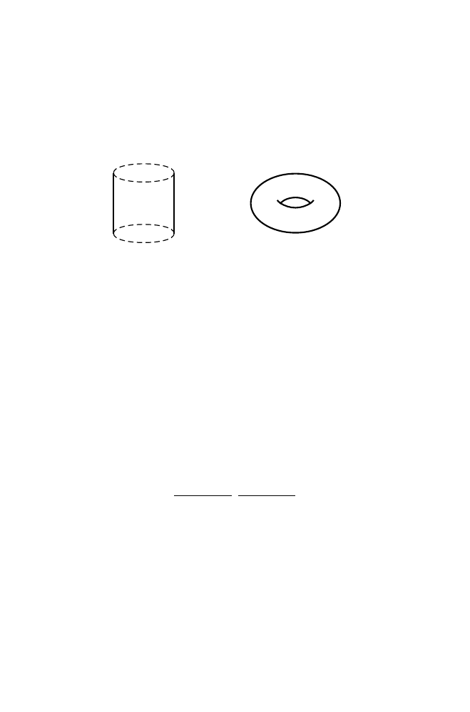
Example 5.18. It follows from Proposition 5.17 that the infinite cylinder S

1

× R and

the torus S

1

× S

1

are manifolds (Figure 5.6).

Infinite cylinder

Torus

Fig. 5.6.

Since M

× N × P = (M × N) × P is the successive product of pairs of spaces,

if M, N and P are manifolds, then so is M

× N × P . Thus, the n-dimensional torus,

S

1

× · · · × S

1

(n times), is a manifold.

Problems

5.1. The real line with two origins
Let A and B be two points not on the real line

R. Consider the set S = (R − {0}) ∪

{A, B}.

A

B

For any two positive real numbers c, d, define

I

A

(

−c, d) = (−c, 0) ∪ {A} ∪ (0, d)

and similarly for I

B

(

−c, d), with B instead of A. Define a topology on S as follows:

On (

R − {0}), use the subspace topology inherited from R, with open intervals as

a basis. A basis at A is the set

{I

A

(

−c, d) | c, d > 0}; similarly, a basis at B is

{I

B

(

−c, d) | c, d > 0}.

54

5 Manifolds

(a) Prove that the map h

: I

A

(

−c, d) −

→ (−c, d) defined by

h(x)

= x for x ∈ (−c, 0) ∪ (0, d),

h(A)

= 0,

is a homeomorphism.

(b) Show that S is locally Euclidean and second countable, but not Hausdorff.

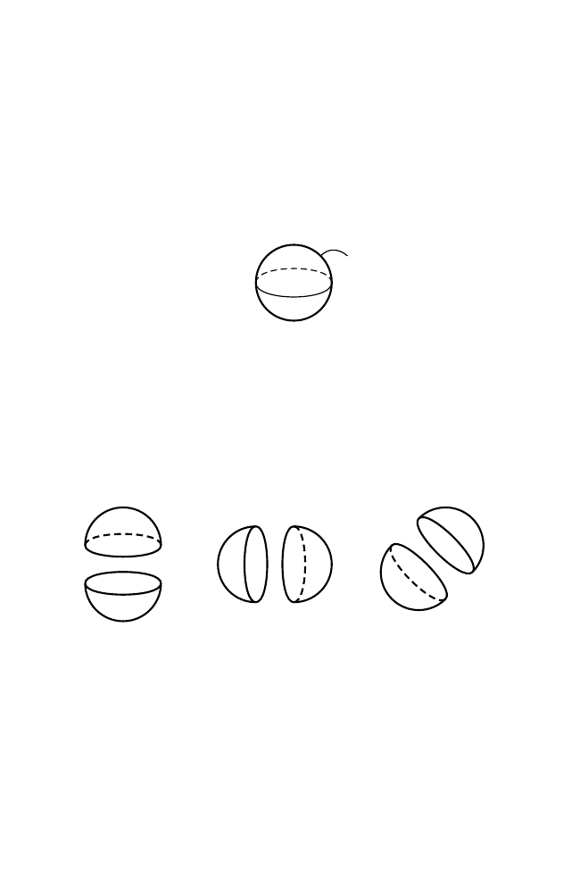
q

Fig. 5.7. Sphere with a hair.

5.2. Sphere with a hair
Prove that the sphere with a hair in

R

3

(Figure 5.7) is not locally Euclidean at q.

Hence it cannot be a topological manifold. (Hint: Mimic Example 5.5.)

U

6

U

5

U

4

U

3

U

1

U

2

Fig. 5.8. Charts on the unit sphere.

5.3. Charts on the sphere
Let S

2

be the unit sphere

x

2

+ y

2

+ z

2

= 1

in

R

3

. Define in S

2

the six charts corresponding to the six hemispheres—the front,

rear, right, left, upper, and lower hemispheres (Figure 5.8):

5.4 Examples of Smooth Manifolds

55

U

1

= {(x, y, z) ∈ S

2

| x > 0},

φ

1

(x, y, z)

= (y, z),

U

2

= {(x, y, z) ∈ S

2

| x < 0},

φ

2

(x, y, z)

= (y, z),

U

3

= {(x, y, z) ∈ S

2

| y > 0},

φ

3

(x, y, z)

= (x, z),

U

4

= {(x, y, z) ∈ S

2

| y < 0},

φ

4

(x, y, z)

= (x, z),

U

5

= {(x, y, z) ∈ S

2

| z > 0},

φ

5

(x, y, z)

= (x, y),

U

6

= {(x, y, z) ∈ S

2

| z < 0},

φ

6

(x, y, z)

= (x, y).

Describe the domain φ

4

(U

14

)

of φ

1 ◦

φ

−1

4

and show that φ

1 ◦

φ

−1

4

is C

∞

on φ

4

(U

14

)

.

Do the same for φ

6 ◦

φ

−1

1

.

5.4. An atlas for a product manifold
Prove Proposition 5.17.