Effective Short-Term Opponent Exploitation in Simplified Poker

Bret Hoehn

Finnegan Southey

Robert C. Holte

University of Alberta, Dept. of Computing Science

Valeriy Bulitko

Centre for Science, Athabasca University

Abstract

Uncertainty in poker stems from two key sources, the

shuffled deck and an adversary whose strategy is un-

known. One approach is to find a pessimistic game theo-

retic solution (i.e. a Nash equilibrium), but human play-

ers have idiosyncratic weaknesses that can be exploited

if a model of their strategy can be learned by observing

their play. However, games against humans last for at

most a few hundred hands so learning must be fast to

be effective. We explore two approaches to opponent

modelling in the context of Kuhn poker, a small game

for which game theoretic solutions are known. Param-

eter estimation and expert algorithms are both studied.

Experiments demonstrate that, even in this small game,

convergence to maximally exploitive solutions in a small

number of hands is impractical, but that good (i.e. better

than Nash or breakeven) performance can be achieved in

a short period of time. Finally, we show that amongst a

set of strategies with equal game theoretic value, in par-

ticular the set of Nash equilibrium strategies, some are

preferable because they speed learning of the opponent’s

strategy by exploring it more effectively.

Introduction

Poker is a game of imperfect information against an ad-

versary with an unknown, stochastic strategy. It rep-

resents a tough challenge to artificial intelligence re-

search. Game theoretic approaches seek to approximate

the Nash equilibrium (i.e. minimax) strategies of the

game (Koller & Pfeffer 1997; Billings et al. 2003),

but this represents a pessimistic worldview where we

assume optimality in our opponent. Human players

have weaknesses that can be exploited to obtain win-

nings higher than the game-theoretic value of the game.

Learning by observing their play allows us to exploit

their idiosyncratic weaknesses. This can be done ei-

ther directly, by learning a model of their strategy, or

indirectly, by identifying an effective counter-strategy.

Several factors render this difficult in practice. First,

real-world poker games like Texas Hold’em have huge

Copyright c

2005, American Association for Artificial Intel-

ligence (www.aaai.org). All rights reserved.

game trees and the strategies involve many parameters

(e.g. two-player, limit Texas Hold’em requires O(10

18

)

parameters (Billings et al. 2003)). The game also has

high variance, stemming from the deck and stochas-

tic opponents, and folding gives rise to partial obser-

vations. Strategically complex, the aim is not simply

to win but to maximize winnings by enticing a weakly-

positioned opponent to bet. Finally, we cannot expect

a large amount of data when playing human opponents.

You may play only 50 or 100 hands against a given op-

ponent and want to quickly learn how to exploit them.

This research explores how rapidly we can gain an

advantage by observing opponent play given that only

a small number of hands will be played in total. Two

learning approaches are studied: maximum a posteri-

ori parameter estimation (parameter learning), and an

“experts” method derived from Exp3 (Auer et al. 1995)

(strategy learning). Both will be described in detail.

While existing poker opponent modelling research

focuses on real-world games (Korb & Nicholson 1999;

Billings et al. ), we systematically study a simpler ver-

sion, reducing the game’s intrinsic difficulty to show

that, even in what might be considered a best case, the

problem is still hard. We start by assuming that the op-

ponent’s strategy is fixed. Tracking a non-stationary

strategy is a hard problem and learning to exploit a

fixed strategy is clearly the first step. Next, we con-

sider the game of Kuhn poker (Kuhn 1950), a tiny game

for which complete game theoretic analysis is available.

Finally, we evaluate learning in a two-phase manner;

the first phase exploring and learning, while the sec-

ond phase switches to pure exploitation based on what

was learned. We use this simplified framework to show

that learning to maximally exploit an opponent in a

small number of hands is not feasible. However, we

also demonstrate that some advantage can be rapidly at-

tained, making short-term learning a winning proposi-

tion. Finally, we observe that, amongst the set of Nash

strategies for the learner (which are “safe” strategies),

the exploration inherent in some strategies facilitates

faster learning compared with other members of the set.

AAAI-05 / 783

J|Q

J|K

Q|J

Q|K

K|J

−1

−2

−2

+1

+1

+1

+1

+1

+2

−1

−1

+2

−1

−2

+2

K|Q

1−β

1−β

β

1−γ

pass

bet

pass

pass

pass

pass

pass

pass

pass

pass

pass

pass

pass

pass

pass

pass

bet

bet

pass

bet

bet

bet

bet

bet

bet

bet

bet

bet

bet

bet

+1

1−η

1−ξ

η

ξ

1−ξ

ξ

α

1−α

1−α

1

1

1

1

1

1

1

1

1

1

β

α

γ

1−γ

γ

η

1−η

Player 1 Choice/Leaf Node

Player 2 Choice Node

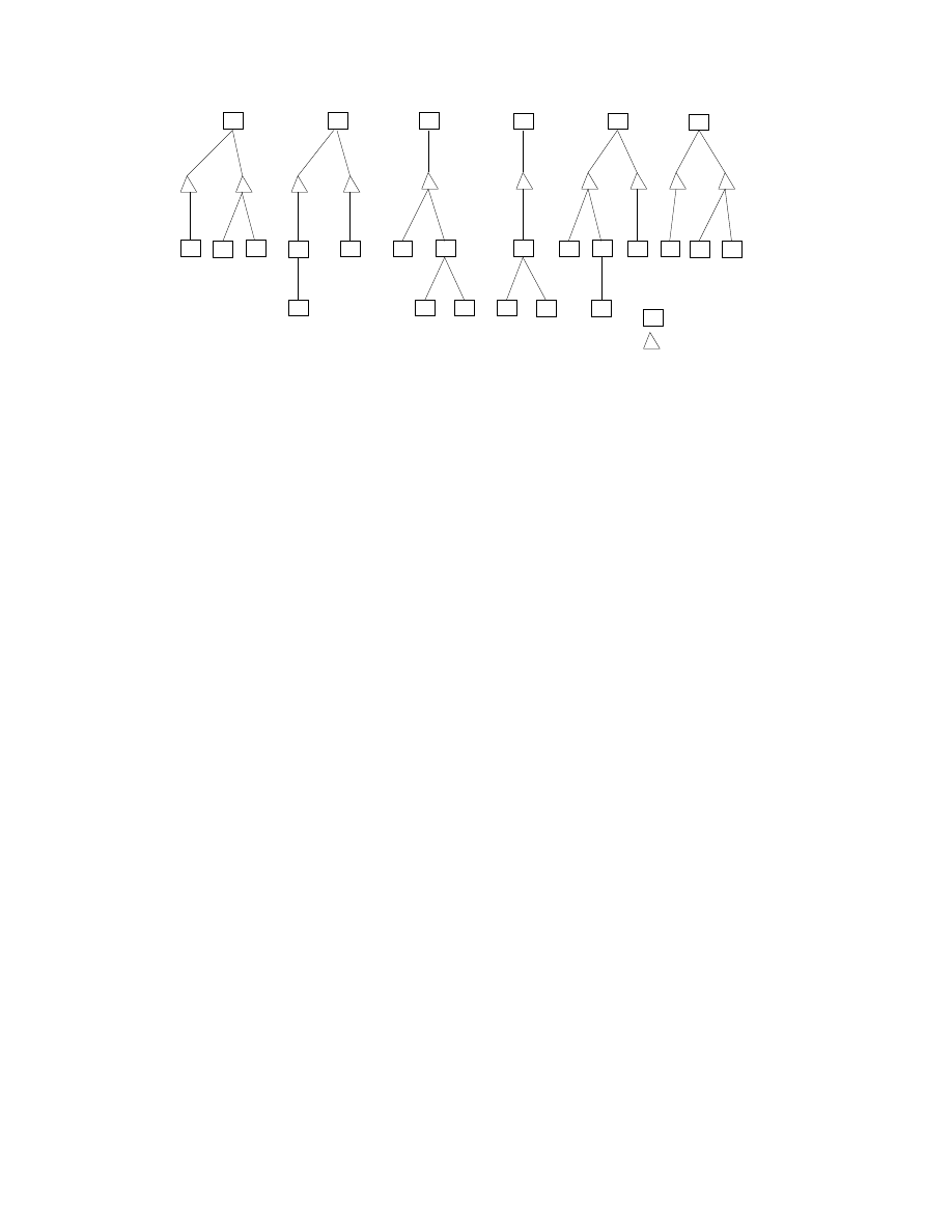
Figure 1: Kuhn Poker game tree with dominated strategies removed

Kuhn Poker

Kuhn poker (Kuhn 1950) is a very simple, two-player

game (P1 - Player 1, P2 - Player 2). The deck consists

of three cards (J - Jack, Q - Queen, and K - King). There

are two actions available: bet and pass. The value of

each bet is 1. In the event of a showdown (players have

matched bets), the player with the higher card wins the

pot (the King is highest and the Jack is lowest). A game

proceeds as follows:
•

Both players initially put an ante of 1 into the pot.

•

Each player is dealt a single card and the remaining

card is unseen by either player.

•

After the deal, P1 has the opportunity to bet or pass.
– If P1 bets in round one, then in round two P2 can:

∗

bet (calling P1’s bet) and the game then ends in a

showdown, or

∗

pass (folding) and forfeit the pot to P1.

– If P1 passes in round one, then in round two P2

can:

∗

bet (in which case there is a third action where P1

can bet and go to showdown, or pass and forfeit

to P2), or

∗

pass (game proceeds to a showdown).

Figure 1 shows the game tree with P1’s value for each

outcome. Note that the dominated strategies have been

removed from this tree already. Informally, a dominated

strategy is one for which there exists an alternative strat-

egy that offers equal or better value in any given situa-

tion. We eliminate these obvious sources of suboptimal

play but note that non-dominated suboptimal strategies

remain, so it is still possible to play suboptimally with

respect to a specific opponent.

The game has a well-known parametrization, in

which P1’s strategy can be summarized by three pa-

rameters (α, β, γ), and P2’s by two parameters (η,

ξ

). The decisions governed by these parameters are

shown in Figure 1. Kuhn determined that the set of

equilibrium strategies for P1 has the form (α, β, γ) =
(γ/3, (1 + γ)/3, γ)

for 0 ≤ γ ≤ 1. Thus, there is a

continuum of Nash strategies for P1 governed by a sin-

gle parameter. There is only one Nash strategy for P2,
η = 1/3

and ξ = 1/3; all other P2 strategies can be

exploited by P1. If either player plays an equilibrium

strategy (and neither play dominated strategies), then

P1 expects to lose at a rate of −1/18 per hand. Thus

P1 can only hope to win in the long run if P2 is playing

suboptimally and P1 deviates from playing equilibrium

strategies to exploit errors in P2’s play. Our discussion

focuses on playing as P1 and exploiting P2, so all ob-

servations and results are from this perspective.

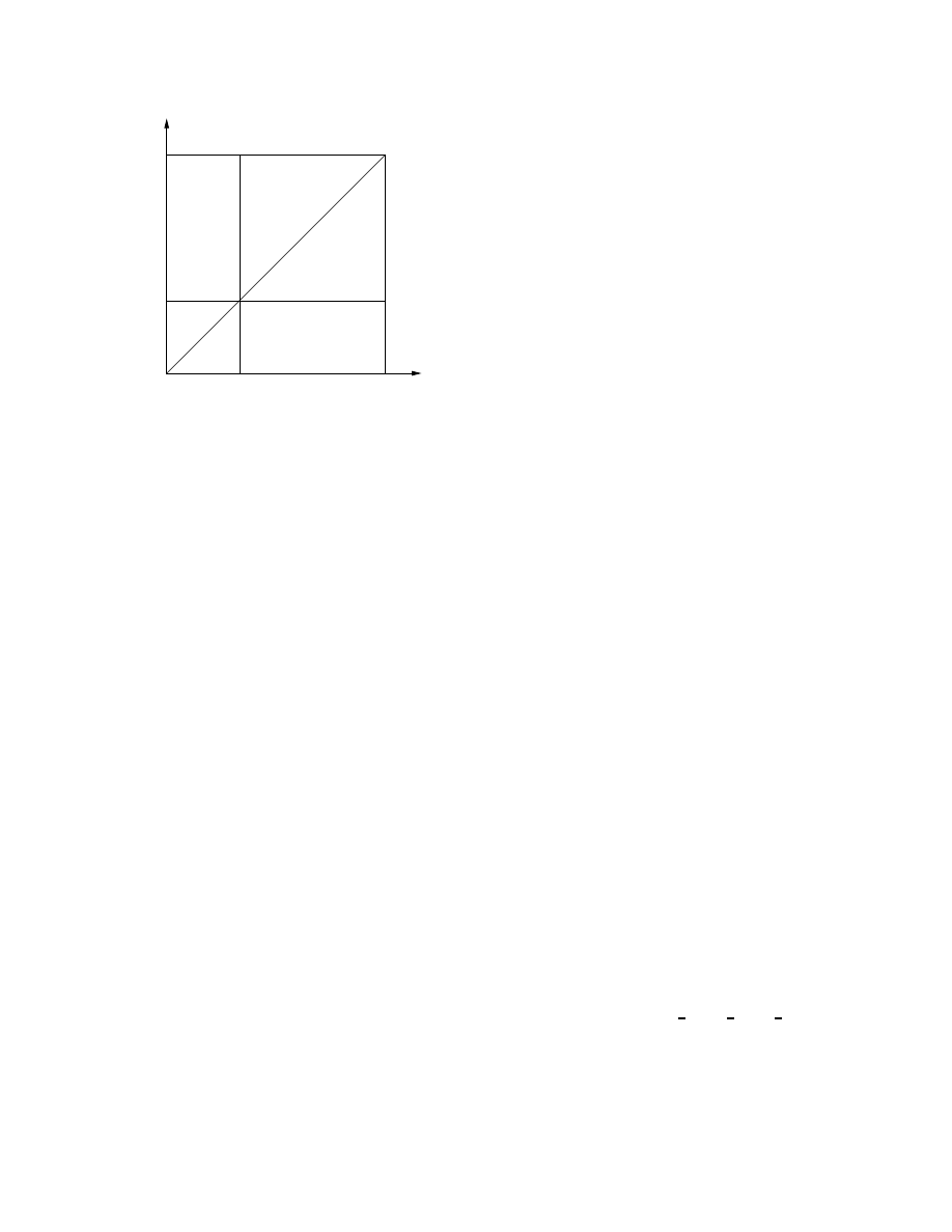
The strategy-space for P2 can be partitioned into the

6 regions shown in Figure 2. Within each region, a sin-

gle P1 pure strategy gives maximal value to P1. For

points on the lines dividing the regions, the bordering

maximal strategies achieve the same value. The in-

tersection of the three dividing lines is the Nash strat-

egy for P2. Therefore, to maximally exploit P2, it is

sufficient to identify the region in which their strat-

egy lies and then to play the corresponding P1 pure

strategy. Note that there are 8 pure strategies for P1:
S

1

= (0, 0, 0), S

2

= (0, 0, 1), S

3

= (0, 1, 0), . . . , S

7

=

(1, 1, 0), S

8

= (1, 1, 1)

. Two of these (S

1

and S

8

) are

never the best response to any P2 strategy, so we need

only consider the remaining six.

This natural division of P2’s strategy space was used

to obtain the suboptimal opponents for our study. Six

opponent strategies were created by selecting a point

at random from each of the six regions. They are
O

1

= (.25, .67), O

2

= (.75, .8), O

3

= (.67, .4), O

4

=

(.5, .29), O

5

= (.25, .17), O

6

= (.17, 2)

. All experi-

ments were run against these six opponents, although

we only have space to show results against representa-

tive opponents here.

AAAI-05 / 784

ξ

1

1/3

1/3

0

S

S

S

S

S

S

1

7

2

6

3

4

5

η

Figure 2: Partition of P2 Strategy-space by Maximal P1

Strategies

Parameter Learning

The first approach we consider for exploiting the op-

ponent is to directly estimate the parameters of their

strategy and play a best response to that strategy. We

start with a Beta prior over the opponent’s strategy and

compute the maximum a posteriori (MAP) estimate of

those parameters given our observations. This is a form

of Bayesian parameter estimation, a typical approach to

learning and therefore a natural choice for our study. In

general poker games a hand either results in a show-

down, in which case the opponent’s cards are observed,

or a fold, which leaves the opponent’s cards uncertain

(we only get to observe their actions, our own cards,

and any public cards). However, in Kuhn poker, the

small deck and dominated strategies conspire in certain

cases to make the opponent’s cards obvious despite their

folding. Thus, certain folding observations (but not all)

contain as much information as a showdown.

The estimation in Kuhn poker is quite straight-

forward because in no case does the estimate of any sin-

gle player parameter depend on an earlier decision gov-

erned by some other parameter belonging to that player.

The task of computing a posterior distribution over op-

ponent strategies for arbitrary poker games is non-trivial

and is discussed in a separate, upcoming paper. For the

present study, the dominated strategies and small deck

again render the task relatively simple.

Priors

We use the Beta prior, which gives a distribution over a

single parameter that ranges from 0 to 1, in our case, the

probability of passing vs. betting in a given situation

(P2 has two parameters, η and ξ). Thus we have two

Beta distributions for P2 to characterize our prior belief

of how they play. A Beta distribution is characterized

by two parameters, θ ≥ 0 and ω ≥ 0. The distribu-

tion can be understood as pretending that we have ob-

served the opponent’s choices several times in the past,

and that we observed θ choices one way and ω choices

the other way. Thus, low values for this pair of param-

eters (e.g. Beta(1,1)) represent a weak prior, easily re-

placed by subsequent observations. Larger values (e.g.

Beta(10,10)) represent a much stronger belief.

A poorly chosen prior (i.e. a bad model of the op-

ponent) that is weak may not cost us much because it

will be quickly overwhelmed by observations. How-

ever, a good prior (i.e. a close model of the opponent)

that is too weak may be thwarted by unlucky observa-

tions early in the game that belie the opponent’s true

nature. We examine the effects of the prior in a later

section. The default prior, unless otherwise specified, is

Beta(1,1) for both η and ξ (i.e. η = 0.5 and ξ = 0.5,

pretending we have seen 2 decisions involving each).

Nash Equilibria and Exploration

Nash equilibrium strategies are strategies for which a

player is guaranteed a certain minimum value regard-

less of the opponent’s strategy. As such, they are “safe”

strategies in the sense that things can’t get any worse.

As mentioned above, the Nash strategies for P1 in Kuhn

poker guarantee a value of −1/18, and thus guarantee

a loss. Against a given P2 strategy, some non-Nash P1

strategy could be better or worse. So, even though Nash

is a losing proposition for P1, it may be better than the

alternatives against an unknown opponent. It therefore

makes sense to adopt a Nash strategy until an opponent

model can be learned. Then the best means of exploit-

ing that model can be tried.

In many games, and in Kuhn Poker P1’s case, there

are multiple equilibrium strategies. We explore the pos-

sibility that some of these strategies allow for faster

learning of an opponent model than others. The exis-

tence of such strategies means that even though they of-

fer identical game theoretic values, some strategies may

be better than others against exploitable opponents.

Another interesting exploration approach is to max-

imize exploration, regardless of the cost. For this, we

employ a “balanced” exploration strategy, (α = 1, β =
1, γ = .5)

, that forces as many showdowns as possible

and equally explores P2’s two parameters.

Strategy Learning

The other learning approach we examine here is what

we will call strategy learning. We can view a strategy

as an expert that recommends how to play the hand.

Taking the six pure strategies shown in Figure 2 plus

a single Nash strategy (α =

1
6

, β =

1
2

, γ =

1
2

)

, we use

the Exp3 algorithm (Auer et al. 1995) to control play by

these experts. Exp3 is a bounded regret algorithm suit-

able for games. It mixes exploration and exploitation

AAAI-05 / 785

Algorithm 1 Exp3

1. Initialize the scores for the K strategies: s

i

= 0

2. For t = 1, 2, . . . until the game ends:

(a) Let the probability of playing the ith strategy for

hand t be p

i

(t) = (1 − ψ)

(1+ρ)

si (t)

P

K
j

=1

(1+ρ)

sj (t)

+

ψ

K

(b) Select the strategy to play u according to the dis-

tribution p and observe the hand’s winnings w.

(c) s

i

(t + 1) =

s

i

(t) +

ψw

Kp

i

(t)

if u = i

s

i

(t)

if u 6= i

in an online fashion to ensure that it cannot be trapped

by a deceptive opponent. Exp3 has two parameters, a

learning rate ρ > 0 and an exploration rate 0 ≤ ψ ≤ 1

(ψ = 1 is uniform random exploration with no online

exploitation). See Algorithm 1 for details.

Exp3 makes very weak assumptions regarding the

opponent so that its guarantees apply very broadly. In

particular, it assumes a non-stationary opponent that can

decide the payoffs in the game at every round. This is

a much more powerful opponent than our assumptions

dictate (a stationary opponent and fixed payoffs). A few

modifications were made to the basic algorithm in or-

der to improve its performance in our particular setting

(note that these do not violate the basic assumptions

upon which the bounded regret results are based).

One improvement, intended to mitigate the effects

of small sample sizes, is to replace the single score

(s

i

) for each strategy with multiple scores, depending

on the card they hold. We also keep a count of how

many times each card has been held. So, instead of

just s

i

, we have s

i,J

, s

i,Q

, and s

i,K

, and counters c

i,J

,

c

i,Q

, and c

i,K

. We then update only the score for the

card held during the hand and increment its counter.

We now compute the expert scores for Algorithm 1’s

probabilistic selection as follows: s

i

=

1
3

s

i,J

/c

i,J

+

1
3

s

i,Q

/c

i,Q

+

1
3

s

i,K

/c

i,K

. This avoids erratic behaviour

if one card shows up disproportionately often by chance

(e.g. the King 10 times and the Jack only once). Natu-

rally, such effects vanish as the number of hands grows

large, but we are specifically concerned with short-term

behaviour. We are simply taking the sum of expecta-

tions instead of the expectation of a sum.

Another improvement is to “share” rewards amongst

those strategies that suggest the same action in a given

situation. We simply update the score and counter for

each agreeing expert. This algorithm bears a strong re-

semblance to Exp4 (Auer et al. 1995).

In all experiments reported here, ρ = 1 and ψ =

0.75

. These values were determined by experimentation

to give good results. Recall that we are attempting to

find out how well it is possible to do, so this parameter

tuning is consistent with our objectives.

Experimental Results

We conducted a large set of experiments using both

learning methods to answer various questions. In partic-

ular, we are interested in how quickly learning methods

can achieve better than Nash equilibrium (i.e. winning

rate ≥ −1/18) or breakeven (i.e. winning rate ≥ 0)

results for P1 , assuming the opponent is exploitable to

that extent. In the former case, P1 is successfully ex-

ploiting an opponent and in the latter, P1 can actually

win if enough hands are played. However, we aim to

play well in short matches, making expected winning

rates of limited interest. Most of our results focus on

the total winnings over a small number of hands (typi-

cally 200, although other numbers are considered).

In our experiments, P1 plays an exploratory strategy

up to hand t, learning during this period. P1 then stops

learning and switches strategies to exploit the opponent.

In parameter learning, the “balanced” exploratory strat-

egy mentioned earlier is used throughout the first phase.

In the second phase, a best response is computed to

the estimated opponent strategy and that is “played” (in

practice, having both strategies, we compute the exact

expected winning rate instead). For strategy learning,

modified Exp3 is run in the first phase, attempting some

exploitation as it explores, since it is an online algo-

rithm. In the second phase, the highest rated expert

plays the remaining hands.

We are chiefly interested in when it is effective to

switch from exploration to exploitation. Our results are

expressed in two kinds of plot. The first kind is a payoff

rate plot, a plot of the expected payoff rate versus the

number of hands before switching, showing the rate at

which P1 will win after switching to exploitation. Such

plots serve two purposes; they show the long-term ef-

fectiveness of the learned model, and also how rapidly

the learner converges to maximal exploitation.

The second kind of plot, a total winnings plot, is

more germane to our goals. It shows the expected total

winnings versus the number of hands before switching,

where the player plays a fixed total number of hands

(e.g. 200). This is a more realistic view of the problem

because it allows us to answer questions such as: if P1

switches at hand 50, will the price paid for exploring be

offset by the benefit of exploitation. It is important to

be clear that the x-axis of both kinds of plot refers to

the number of hands before switching to exploitation.

All experiments were run against all six P2 oppo-

nents selected from the six regions in Figure 2. Only

representative results are shown here due to space con-

straints. Results were averaged over 8000 trials for pa-

rameter learning and 2000 trials for strategy learning.

The opponent is O

6

unless otherwise specified, and is

typical of the results obtained for the six opponents.

Similarly, results are for parameter learning unless oth-

erwise specified, and consistent results were found for

strategy learning, albeit with overall lower performance.

AAAI-05 / 786

-0.12

-0.1

-0.08

-0.06

-0.04

-0.02

0

0.02

0.04

0.06

0

100

200

300

400

500

600

700

800

900

Expected Payoff Rate

Switching Hand

Paramater Learning

Strategy Learning

Maximum

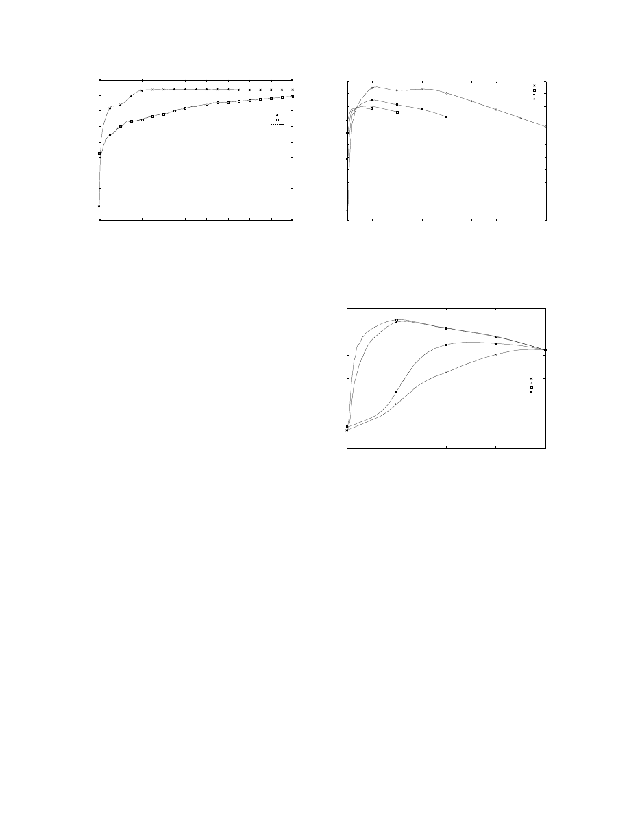
Figure 3: Convergence Study: Expected payoff rate vs.

switching hand for parameter and strategy learning

Convergence Rate Study

Figure 3 shows the expected payoff rate plot of the

two learning methods against a single opponent. The

straight-line near the top shows the maximum exploita-

tion rate for this opponent (i.e. the value of the best re-

sponse to P2’s strategy). It takes 200 hands for param-

eter learning to almost converge to the maximum and

strategy learning does not converge within 900 hands.

Results for other opponents are generally worse, requir-

ing several hundred hands for near-convergence. This

shows that, even in this tiny game, one cannot expect

to achieve maximal exploitation in a small number of

hands. The possibility of maximal exploitation in larger

games can reasonably be ruled out on this basis and we

must adopt more modest goals for opponent modellers.

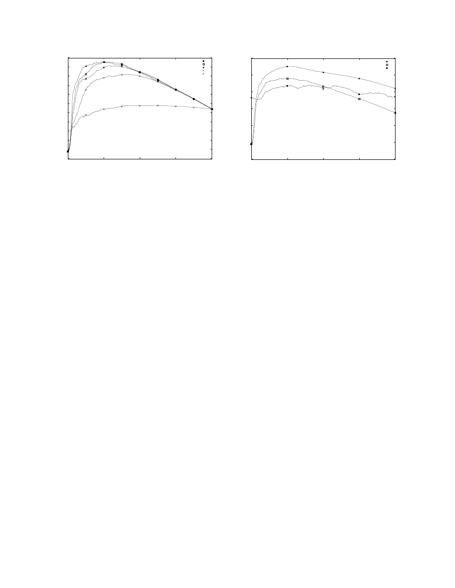
Game Length Study

This study is provided to show that our total winnings

results are robust to games of varying length. While

most of our results are presented for games of 200

hands, it is only natural to question whether different

numbers of hands would have different optimal switch-

ing points. Figure 4 shows overlaid total winnings plots

for 50, 100, 200, and 400 hands using parameter learn-

ing. The lines are separated because the possible to-

tal winnings is different for differing numbers of hands.

The important observation to make is that the highest

value regions of these curves are fairly broad, indicat-

ing that switching times are flexible. Moreover, the re-

gions of the various curves overlap substantially. Thus,

switching at hand 50 is a reasonable choice for all of

these game lengths, offering close to the best possible

total winnings in all cases. This means that even if

we are unsure, a priori, of the number of hands to be

played, we can be confident in our choice of switching

time. Moreover, this result is robust across our range of

opponents. A switch at hand 50 works well in all cases.

-45

-40

-35

-30

-25

-20

-15

-10

-5

0

5

10

0

50

100

150

200

250

300

350

400

Expected Total Winnings

Switching Hand

Horizon 50

Horizon 100

Horizon 200

Horizon 400

Figure 4: Game Length Study: Expected total winnings

vs. switching hand for game lengths of 50, 100, 200,

and 400 hands played by parameter learning

-25

-20

-15

-10

-5

0

5

0

50

100

150

200

Expected Total Winnings

Switching Hand

weak, bad

strong, bad

weak, default

strong, default

Figure 5: Prior Study: Four different priors for parame-

ter learning against a single opponent.

Parameter Learning Prior Study

In any Bayesian parameter estimation approach, the

choice of prior is clearly important. Here we present a

comparison of various priors against a single opponent

(O

6

= (.17, .2)

). Expected total winnings are shown

for four priors: a weak, default prior of (.5,.5), a weak,

bad prior of (.7,.5), a strong, default prior of (.5,.5), and

a strong, bad prior of (.7,.5). The weak priors assume

2 fictitious points have been observed and the strong

priors assume 20 points. The “bad” prior is so called

because it is quite distant from the real strategy of this

opponent. Figure 5 shows that the weak priors clearly

do better than the strong, allowing for fast adaptation to

the correct opponent model. The strong priors perform

much more poorly, especially the strong bad prior.

AAAI-05 / 787

-22

-20

-18

-16

-14

-12

-10

-8

-6

-4

-2

0

0

50

100

150

200

Expected Total Winnings

Switching Hand

Gamma = 1.0

Gamma = 0.75

Gamma = 0.5

Gamma = 0.25

Gamma = 0

Figure 6: Nash Study: Expected total winnings vs.

switching hand for parameter learning with various

Nash strategies used during the learning phase.

Nash Exploration Study

Figure 6 shows the expected total winnings for param-

eter learning when various Nash strategies are played

by the learner during the learning phase. The strate-

gies with larger γ values are clearly stronger, more ef-

fectively exploring the opponent’s strategy during the

learning phase. This advantage is typical of Nash strate-

gies with γ > 0.7 across all opponents we tried.

Learning Method Comparison

Figure 7 directly compares strategy and parameter

learning (both balanced and Nash exploration (γ = 1)),

all against a single opponent. Balanced parameter learn-

ing outperforms strategy learning substantially for this

opponent. Over all opponents, either the balanced or the

Nash parameter learner is the best, and strategy learning

is worst in all but one case.

Conclusions

This work shows that learning to maximally exploit an

opponent, even a stationary one in a game as small as

Kuhn poker, is not generally feasible in a small num-

ber of hands. However, the learning methods explored

are capable of showing positive results in as few as

50 hands, so that learning to exploit is typically bet-

ter than adopting a pessimistic Nash equilibrium strat-

egy. Furthermore, this 50 hand switching point is ro-

bust to game length and opponent. Future work includes

non-stationary opponents, a wider exploration of learn-

ing strategies, and larger games. Both approaches can

scale up, provided the number of parameters or experts

is kept small (abstraction can reduce parameters and

small sets of experts can be carefully selected). Also,

the exploration differences amongst equal valued strate-

gies (e.g. Nash) deserves more attention. It may be pos-

-25

-20

-15

-10

-5

0

5

0

50

100

150

200

Expected Total Winnings

Switching Hand

Parameter Learning

Nash (Gamma = 1)

Strategy Learning

Figure 7: Learning Method Comparison: Expected total

winnings vs. switching hand for both parameter learn-

ing and strategy learning against a single opponent.

sible to more formally characterize the exploratory ef-

fectiveness of a strategy. We believe these results should

encourage more opponent modelling research because,

even though maximal exploitation is unlikely, fast op-

ponent modelling may still yield significant benefits.

Acknowledgements

Thanks to the Natural Sciences and Engineering Re-

search Council of Canada and the Alberta Ingenuity

Centre for Machine Learning for project funding, and

the University of Alberta poker group for their insights.

References

Auer, P.; Cesa-Bianchi, N.; Freund, Y.; and Schapire,

R. E. 1995. Gambling in a rigged casino: the adversar-

ial multi-armed bandit problem. In Proc. of the 36th

Annual Symp. on Foundations of Comp. Sci., 322–331.
Billings, D.; Davidson, A.; Schauenberg, T.; Burch,

N.; Bowling, M.; Holte, R.; Schaeffer, J.; and Szafron,

D. Game Tree Search with Adaptation in Stochas-

tic Imperfect Information Games. In Computers and

Games’04.
Billings, D.; Burch, N.; Davidson, A.; Holte, R.; Scha-

effer, J.; Schauenberg, T.; and Szafron, D. 2003. Ap-

proximating game-theoretic optimal strategies for full-

scale poker. In 18th Intl. Joint Conf. on Artificial In-

telligence (IJCAI’2003).
Koller, D., and Pfeffer, A. 1997. Representations and

solutions for game-theoretic problems. Artificial Intel-

ligence 94(1):167–215.
Korb, K., and Nicholson, A. 1999. Bayesian poker. In

Uncertainty in Artificial Intelligence, 343–350.
Kuhn, H. W. 1950. A simplified two-person poker.

Contributions to the Theory of Games 1:97–103.

AAAI-05 / 788