Combustion, Explosion, and Shock Waves, Vol. 37, No. 5, pp. 523–534, 2001

Parametric Analysis of the Simplest Model of the Theory

of Thermal Explosion — the Zel’dovich–Semenov Model

UDC 536.46

V. I. Bykov

1

and S. B. Tsybenova

2

Translated from Fizika Goreniya i Vzryva, Vol. 37, No. 5, pp. 36–48, September–October, 2001.
Original article submitted May 5, 2000; revision submitted March 5, 2001.

Parametric analysis is performed for the Zel’dovich–Semenov model, a basic model of
the theory of thermal explosion that describes the dynamics of an exothermic reaction
with arbitrary kinetics in a continuous stirred tank reactor. Particular attention is
given to the cases of first- and nth-order reactions, oxidation reaction, and reaction
with arbitrary kinetics. Parametric dependences of steady states on dimensionless
parameters, curves of multiplicity and neutrality of steady states, and parametric and
phase portraits of the system are constructed. Regions of multiple steady states and
self-oscillations and a region of technological safety are distinguished.

INTRODUCTION

The mathematical model of a thermal explosion in

a medium with averaged parameters (continuous stirred
tank reactor) has been a traditional subject of investiga-
tion in combustion theory [1–8]. It can be said that the
present-day stage of its parametric analysis was origi-
nated in [1]. Vaganov, Samoilenko, and Abramov [4] de-
termined 35 different phase portraits of the correspond-
ing dynamic system. The diversity of the dynamic be-
havior of this model was shown in detail in [5, 6, 9, 10].
Construction of bifurcation curves which divide a pa-
rameter plane into regions of different dynamic behav-
ior of the system and analysis of their evolution with a
third parameter varied provide additional information
on the character of the critical phenomena in the pro-
cesses considered.

In the present paper, we perform a parametric anal-

ysis of the model of an exothermic reaction carried out
in a continuous stirred tank reactor. In contrast to pre-
vious publications, where the corresponding paramet-
ric portraits are given schematically, as a rule, in one
of the chosen planes of dimensionless parameters, we
construct local bifurcation curves for all possible com-
binations of the parameters. With allowance for the

1

Institute of Computational Modeling,
Siberian Division, Russian Academy of Sciences,
Krasnoyarsk 660036.

2

Krasnoyarsk State Technical University,
Krasnoyarsk 660074.

specific features of the models, they are written explic-
itly. From the practical viewpoint, results of analysis of
local bifurcations are sufficient to determine the main
characteristics of the dynamic process.

In addition to the first-order reaction, we consider

more general kinetic relations. Particular consideration
is given to the special cases of the widely used reaction
schemes: A + O

2

→ P, nA → P, and nA + O

2

→ P,

where A is the reactant and P is the reaction product.
If possible, the critical conditions [curves of change in
the number of steady states (SS) and in the type of their
stability] are explicitly written throughout. The results
obtained allow one to estimate the effect of kinetic fea-
tures on the critical ignition conditions, the existence of
multiple SS and self-oscillation combustion regimes.

The universal procedure of parametric analysis

makes it possible to develop effective numerical algo-
rithms for constructing parametric relations and bifur-
cation curves in the cases where corresponding analyt-
ical expressions cannot be obtained. Results of para-
metric analysis of some basic models were used to de-
sign an information system in the form of a model bank.
This system combines both the results of analysis of the
models considered and technologies of parametric anal-
ysis that allow one to study new models and incorporate
them together with results of numerical and qualitative
analyses in the model bank.

0010-5082/01/3705-0523 $25.00 c

2001

Plenum Publishing Corporation

523

524

Bykov and Tsybenova

The procedure of parametric analysis [11–15] in-

cludes investigation of the number of SS of the initial
mathematical model, their stability analysis, construc-
tion of dependences of steady-state characteristics on
parameters, determination of local bifurcation curves
(curves of multiplicity and neutrality of SS), construc-
tion of parametric and phase portraits of the dynamic
system investigated, and calculation of time depen-
dences of its solutions.

MATHEMATICAL MODEL

In a continuous stirred tank reactor, the model of

a first-order exothermic reaction

A

→ P,

has the form

V

dX

dt

=

−V k(T )X + q(X

0

− X),

c

p

ρV

dT

dt

= (

−∆H)V k(T )X

+ qρc

p

(T

0

− T ) + hS(T

w

− T ), (1)

k(T ) = k

0

exp

− E/RT

,

where V [cm

3

] is the volume of the reactor, k(T ) [sec

−1

]

is the reaction rate constant, E [J/mole] is the activa-
tion energy, R [J/(mole

· K)] is the universal gas con-

stant, k

0

is the preexponent, X and X

0

[mole/cm

3

] are

the current and inlet concentrations of the reagent, re-
spectively, T and T

0

[K] are the current and inlet tem-

peratures of the mixture, respectively, q [cm

3

/sec] is the

volume flow rate, ρ [mole/cm

3

] is the density of the mix-

ture, c

p

[J/(mole

· K] is the specific heat of the reactive

mixture, S [cm

2

] is the area of the heat-exchange sur-

face, h [J/(cm

2

· sec · K)] is the coefficient of heat transfer

through the reactor wall, (

−∆H) [J/mole] is the ther-

mal effect of the reaction, t [sec] is astronomical time,
and T

w

[K] is the temperature of the reactor walls.

Following Frank-Kamenetskii [16], we introduce

the dimensionless parameters and variables:

T

∗

=

hST

w

+ c

p

ρqT

0

hS + c

p

ρq

,

α

∗

= h +

c

p

ρq

S

,

Da = (V /q) k(T

0

),

Se =

(

−∆H)ρ

α

∗

(S/V )

E

RT

∗2

k

0

exp

−

E

RT

∗

,

β =

(

−∆H)X

0

c

p

ρT

0

,

γ =

E

RT

0

,

x =

X

0

− X

X

0

,

y =

E

RT

2

(T

− T

∗

),

τ = k

0

t exp

−

E

RT

∗

.

We assume that the initial and inlet conditions for

the reactor coincide:

X(0) = X

0

,

qρc

p

(T

0

− T (0)) = hS(T (0) − T

w

).

Model (1) can be written in dimensionless form:

dx

dτ

= f (x) exp

y

1 + βy

−

x

Da

= f

1

(x, y),

γ

dy

dτ

= f (x) exp

y

1 + βy

−

y

Se

= f

2

(x, y).

(2)

Here f (x) = 1

−x is a first-order kinetic function, x and

y are the dimensionless concentration and temperature,
respectively, and Da, Se, β, and γ are dimensionless pa-
rameters. This model is called the Zel’dovich–Semenov
model.

PARAMETRIC ANALYSIS
FOR THE FIRST-ORDER REACTION

Steady States. The steady states of system (2)

are solutions of the equations

f

1

(x, y) = 0,

f

2

(x, y) = 0.

(3)

Summing Eqs. (3), we express x in terms of y:

x = (Da/Se) y

or

x = νy,

where ν = Da/Se. The second equation in (3) yields

1

− y

Da

Se

exp

y

1 + βy

=

y

Se

.

(4)

The steady states are determined from Eq. (4), in

which the right side is the heat-release function F (y)
and the left side is the heat-removal function P (y):

F (y) = 1

− y Da/Se

e(y),

P (y) = y/Se.

Here e(y) = exp(y/(1 + βy)).

The SS of system (2) are studied with the help

of Semenov’s diagram, which shows the dependences of
the heat-release and heat-removal functions on the tem-
perature of the substance in the reactor. The points of
intersection of the curves of F (y) and P (y) specify the
temperature y in the SS. The steady-state concentra-
tions are x = νy. The necessary and sufficient condition
for the uniqueness of SS is given by 1/Se = P

0

> F

0

, i.e.,

the heat-removal rate must be greater than the heat-
release rate in the SS.

Parametric Dependences.

The dimensionless

parameters Da, Se, and β enter into the steady-state
equation (4) in a linear manner, and therefore, we can
write parametric dependences of the form Da = Da (y),
Se = Se(y), etc.

Parametric Analysis of the Simplest Model of the Zel’dovich–Semenov Model

525

Fig. 1. Steady-state temperature versus the parameter
β for Da = 0.03 (dashed curves refer to unstable SS).

From (4), we obtain, for example, the expression

Se (y) = (Da + 1/e(y))y.

(5)

Similarly, we obtain parametric dependences for the re-
maining parameters:

Da (y) =

Se

y

−

1

e(y)

,

(6)

β(y) =

1

ln(y/(Se

− Da y))

−

1

y

,

(7)

ν(y) =

1

y

−

1

e(y) Se

.

Constructing the dependence Da(y) in accordance

with (6), we obtain the inverse function of the desired
parametric dependence y = y(Da). If (6) is specified
graphically, the necessary value of y is readily deter-
mined for any fixed value of Da. Figure 1 shows an
example of dependence (7). The dashed curves refer to
unstable SS.

Type of Stability of Steady States. The type

of stability of the steady states is determined by the
roots of the characteristic equation λ

2

− σλ + ∆ = 0,

where σ and ∆ are found with the use of the Jacobi
matrix elements:

a

11

=

∂f

1

∂x

=

−e(y) −

1

Da

,

a

12

=

∂f

1

∂y

=

e(y)f (x)

(1 + βy)

2

,

a

21

=

∂f

2

∂x

=

−e(y)

γ

,

(8)

a

22

=

∂f

2

∂y

=

e(y)f (x)

γ(1 + βy)

2

−

1

γSe

,

i.e., σ = a

11

+ a

22

and ∆ = a

11

a

22

− a

12

a

21

.

Multiplicity Curves.

A multiplicity curve

L

∆

(∆ = 0) is the boundary that divides a parameter

plane into regions with one and three SS. We consider,
for example, the (Da, Se) plane and write the equation
of the multiplicity curve L

∆

. To this end, it is necessary

to solve the system

f

1

(x, y, Da, Se) = 0,

f

2

(x, y, Da, Se) = 0,

(9)

∆(x, y, Da, Se) = 0.

Using (4), we reduce (9) to the system

G(y, Da, Se) = 0,

∆(y, Da, Se) = 0.

(10)

Substituting the explicit expression of Se(y, Da)

into the second equation of (10), we obtain the follow-
ing equation for the boundary of the region of multiple
SS in the (Da, Se) plane:

L

∆

(Da, Se):















Da (y) =

y

− (1 + βy)

2

(1 + βy)

2

e(y)

,

Se (y, Da) =

Da +

1

e(y)

y.

(11)

Similarly, we determine the multiplicity curve L

∆

in the

(Se, ν) plane:

L

∆

(Se, ν):















Se(y) =

y

2

(1 + βy)

2

e(y)

,

ν(y, Se) =

1

y

−

1

e(y)Se

.

(12)

For the planes of parameters including γ, the mul-

tiplicity curves are two parallel lines that determine
the region of existence of three SS in the correspond-
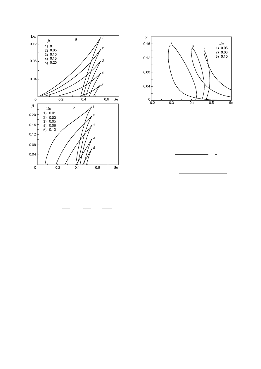
ing plane. Figure 2a shows some multiplicity curves in
the (Da, Se) plane.

In the case where it is difficult to obtain explicit

expressions for multiplicity curves in some parameter
planes, one can use a graphical procedure for construct-
ing L

∆

. It consists of constructing a number of para-

metric dependences for one parameter with a second
parameter varied. We note that such dependences can
be constructed for all parameters. The interval of multi-
ple SS lies between the turning points of the parametric
curve (maximum and minimum values of the curves).
The boundaries of this interval specify the region of mul-
tiple SS in the corresponding plane with variation of a
second parameter. Figure 2b shows results obtained by
the graphical procedure described above.

Neutrality Curves.

A neutrality curve L

σ

(σ = 0) specifies the type of stability of a SS. To con-
struct L

σ

, it is necessary to solve the system

G(y, Da, Se) = 0,

σ(y, Da, Se) = 0.

(13)

Substituting the explicit expression for Da(y, Se)

(6) into the second equation of (13), we obtain the ex-
plicit equation for L

σ

:

526

Bykov and Tsybenova

Fig. 2. Multiplicity curves.

L

σ

(Da, Se):











Da (y) =

a

e(y)

±

s

a

e(y)

2

−

1

e

2

(y)

,

Se (y, Da (y)) = Da + 1/e(y)

y,

(14)

where a(y) = 1/2γ(1 + βy)

2

− 1/2γy − 1. Similarly, we

obtain L

σ

in the other parameter planes:

L

σ

(Se, ν):











Se (y) =

Da (y

− (1 + βy)

2

)

y(1 + βy)

2

(Da e(y) + 1)

,

ν(y, Se) = 1/y

− 1/e(y)Se;

L

σ

(γ, Da):











γ(y, Da) =

Da e(y)(y

− (1 + βy)

2

)

y(1 + βy)

2

(Dae(y) + 1)

2

,

Da (y) = Se/y

− 1/e(y);

(15)

L

σ

(γ, Se):











γ(y, Se) =

(e(y)Se

− y)(y − (1 + βy)

2

)

e

2

(y)Se

2

(1 + βy)

2

,

Se (y) = Da + 1/e(y)

y;

Fig. 3. Neutrality curves in the (Se, γ) plane for β =
0.01.

L

σ

(γ, β):















γ(y, β) =

Da e(y)(y

− (1 + βy)

2

)

y(1 + βy)

2

(Da e(y) + 1)

2

,

β(y) =

1

ln(y/(Se

− Da y))

−

1

y

;

L

σ

(γ, ν):











γ(y, ν) =

νe(y)Se (y

− (1 + βy)

2

)

y(1 + βy)

2

(e(y)νSe + 1)

2

,

ν(y) = 1/y

− 1/e(y)Se.

Figure 3 shows some neutrality curves in the (Se,γ)
plane obtained by varying a third parameter.

If explicit expressions for the neutrality curves in

some parameter planes are difficult to obtain, one can
construct L

σ

by a graphical procedure, as is done above.

Parametric dependences for one of the parameters are
constructed in a similar manner by varying a second
parameter. The points corresponding to the change in
sign of σ are plotted in the parameter plane.

Parametric Portraits. The relative position of

the multiplicity L

∆

and neutrality curves L

σ

specifies

the parametric portrait of the system. It specifies para-
metric regions with different numbers of SS and different
types of their stability. In our case, a total of up to six
such regions exist (Fig. 4).

Phase Portraits. In accordance with the para-

metric portrait (see Fig. 4), one can distinguish six
types of phase portraits [8].

Region 1 is character-

ized by a single stable SS (low-temperature or high-
temperature state). Regions 2 and 6 correspond to un-
stable SS, which ensure the presence of self-oscillations
in the system. They differ in that in region 2 one SS
exists, whereas in region 6 three SS exist. In regions
3–5 also three SS exist. Region 3 is characterized by

Parametric Analysis of the Simplest Model of the Zel’dovich–Semenov Model

527

Fig. 4. Parametric portrait in the (Se, Da) plane for
β = 0.05 and γ = 0.01 (regions 1–6 are described in
the text).

Fig. 5. Steady-state temperature versus time for
Da = 0.14, Se = 0.6, β = 0, γ = 0.035, x(0) = 0, and
y(0) = 0.

one unstable and two stable low- and high-temperature
SS. Regions 4 and 5 correspond to one stable and two
unstable SS.

Time Dependences.

Numerical integration of

the initial dynamic system (2) yields time dependences
x(t) and y(t) for different initial conditions and varied
parameters. Figure 5 shows an example of time depen-
dence.

Regions of Technological Safety Regimes. An

analysis of time dependences and phase portraits shows
that transition of solutions to a low-temperature SS
can be accompanied by a substantial dynamic “over-
shoot” (abrupt increase in temperature at a certain
time), which is undesirable from the technological view-
point. For other initial data and parameters of the sys-
tem, transition of solutions to SS can be of a monotonic
character.

In the corresponding parametric portrait,

this region (region 1a in Fig. 6) is distinguished and
presented as the region of technological safety regimes.
We note that it depends strongly on the initial data and
other parameters of the system.

Fig. 6. Regions of low-temperature (1a) and high-
temperature (1b) regimes in the parametric portrait
in the (Se,Da) plane for β = 0.05 and γ = 0.025.

OXIDATION REACTION A + O

2

→ P

In the simplest case of modeling combustion pro-

cesses, it is assumed that oxygen is present in ex-
cess [10]. In some cases, however, this assumption is
not justified, and the oxidizer must be included in the
reaction scheme. Therefore, we consider the oxidation
reaction

A + O

2

→ P,

where A is the initial gaseous substance and P is the
combustion product.

For this reaction scheme, the mathematical model

of a continuous stirred tank reactor has the form

V

dX

A

dt

=

−V k(T )X

A

X

O

2

+ q(X

0

A

− X

A

),

V

dX

O

2

dt

=

−V k(T )X

A

X

O

2

+ q(X

0

A

− X

A

),

(16)

c

p

ρV

dT

dt

= (

−∆H

p

)V k(T )X

A

X

O

2

+ qρc

p

(T

0

− T ) + hS(T

w

− T ),

where X

A

and X

O

2

are the concentrations of the

reagents.

Under the assumption of identical initial and inlet

conditions

X

A

(0)

− X

0

A

= X

O

2

(0)

− X

0

O

2

,

qρc

p

(T

0

− T (0)) = hS(T (0) − T

w

),

model (16) can be written in dimensionless form (ac-
cording to Frank-Kamenetskii):

dx

dt

= f (x)(1

− αx)e(y) −

x

Da

= f

1

(x, y),

(17)

γ

dy

dt

= f (x)(1

− αx)e(y) −

y

Se

= f

2

(x, y),

528

Bykov and Tsybenova

where f (x) = 1

−x, e(y) = exp(y/(1+βy)), and α is the

dimensionless parameter that characterizes the fuel-to-
oxygen ratio. The remaining dimensionless parameters
are defined as in model (2).

Steady States. The steady states (17) are deter-

mined from the system

(1

− x)(1 − αx)e(y) − x/Da = 0,

(18)

(1

− x)(1 − αx)e(y) − y/Se = 0.

Expressing x from the first equation of system (18) and
substituting it into the second equation, we obtain the
steady-state equation

1

− y

Da

Se

1

− α

Da

Se

e(y) =

y

Se

,

(19)

where the heat-release and heat-removal functions are
given by

F (y) = (1

− νy)(1 − ανy)e(y),

P (y) = y/Se.

As before, ν = Da/Se. In contrast to the simplest model
[system (2)], we now have five dimensionless parame-
ters. Here we give particular attention to the effect of
the parameter α on the steady-state and dynamic char-
acteristics of the model.

Type of Stability of Steady States. We study

the stability of SS by the standard procedure. Recall
that the critical conditions for dynamic systems in a
plane are given by the equality to zero of the coeffi-
cients of the characteristic equation σ and ∆, which are
expressed in terms of the Jacobi matrix elements:

a

11

=

∂f

1

∂x

= (2αx

− α − 1)e(y) −

1

Da

,

a

12

=

∂f

1

∂y

=

(1

− x)(1 − αx)e(y)

(1 + βy)

2

,

(20)

a

21

=

∂f

2

∂x

=

(2αx

− α − 1)e(y)

γ

,

a

22

=

∂f

2

∂y

=

(1

− x)(1 − αx)e(y)

γ(1 + βy)

2

)

−

1

γSe

.

Parametric Dependences. As before, the form

of the functions F and P for (19) allows one to obtain
explicit dependences of SS on various parameters (more
precisely, their inverse dependences):

Da (y) =

Se

2y

1 +

1

α

−

s

Se

2y

1 +

1

α

2

−

Se

αy

Se

y

−

1

e(y)

,

Fig. 7. Steady-state temperature versus the param-
eter α for Da = 0.05 and β = 0.01.

Se (y) =

Da y

2

(1 + α) +

y

2e(y)

+

s

Da y

2

(1 + α) +

y

2e(y)

2

− αDa

2

y

2

,

β(y) =

1

ln(Se y/(Se

− Da y)(Se − αDa y))

−

1

y

,

(21)

ν(y) =

1

2y

1 +

1

α

−

s

1

2y

1 +

1

α

2

−

1

αy

1

y

−

1

e(y)Se

,

α(y) =

Se

Da

1

y

−

1

e(y)(Se

− Da y)

.

The dependences of steady-state concentrations on the
parameters of the system can be written similarly to
(21).

Figure 7 shows results of calculation by one of the

formulas (21) with one varied parameter. Dependences
of steady-state concentrations on the parameters can be
calculated by the formulas in a similar manner. Hav-
ing dependences in explicit form, one can readily ana-
lyze the effect of the remaining parameters on steady-
state characteristics. For example, an analysis of the
dependence of the steady-state temperature of combus-
tion on the parameter Se for α varied shows that the
region of multiple SS reduces as the fuel-to-oxygen ra-
tio increases. It becomes maximal for excess in oxygen
(α = 0) and vanishes for α > 2 (with the remaining
parameters fixed). The same effect is observed for the
dependence of the temperature on the parameter Da.

Parametric Analysis of the Simplest Model of the Zel’dovich–Semenov Model

529

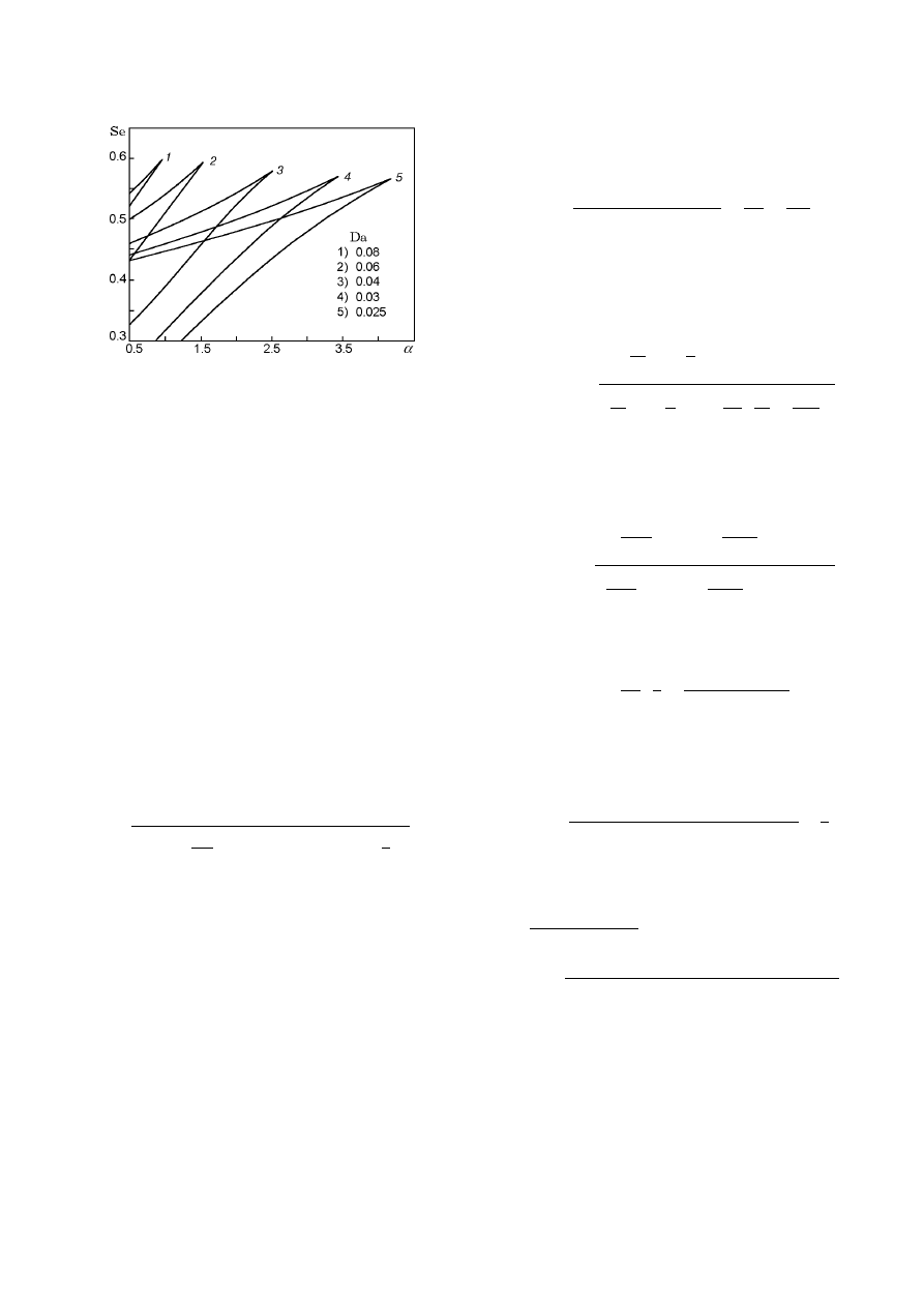
Fig. 8. Multiplicity curves in the (α, Se) plane for
β = 0.05.

Multiplicity Curves. The multiplicity curve L

∆

,

which specifies the change in the number of SS, is ob-
tained from the system

F (y, ξ)

− P (y, ξ) = 0,

∆(y, ξ) = 0,

(22)

where ξ is a parameter vector, the first equation cor-
responds to the steadiness condition, and the second
equation to the criticality condition. We write system
(22) in the form

(1

− νy)(1 − ανy)e(y) − y/Se = 0,

(23)

(1

− νy)(1 − ανy)e(y)/(1 + βy)

2

+ (2ανy

− α − 1)νe(y) − 1/Se = 0. (24)

Using (23) and (24), we obtain the equation of the mul-
tiplicity curve in the (Se,α) plane:

L

∆

(Se, α):



















Se(y) = Da y + 1/2bc

+

r

Da y +

1

2bc

2

− Da

Da y

2

+ c

1 +

y

b

,

α = α(y, Se).

(25)

Here b = (1 + βy)

2

and c = y

2

/e(y). For the remain-

ing parameter planes, explicit formulas of the type (25)
become very cumbersome and are not given here. An
example of constructing dependences (25) by varying
a third parameter is given in Fig. 8. Complicated cal-
culations can be avoided by using the above-mentioned
graphical procedure for constructing multiplicity curves
from the known parametric dependences (21).

Neutrality Curves. To construct the neutrality

curve L

σ

, which specifies the change in the type of sta-

bility of SS, one need to solve the system

(1

− νy)(1 − ανy)e(y) − y/Se = 0,

(26)

(2ανy

− α − 1)e(y)

+

(1

− νy)(1 − ανy)e(y)

γ(1 + βy)

2

−

1

Da

−

1

γSe

= 0.

Substituting α(y) from the first equation of system

(26) into the second equation, we obtain the following
expressions for the neutrality curves in the (γ, ξ) planes:

L

σ

(γ, Da):































Da (y) =

Se

2y

1 +

1

α

+

s

Se

2y

1 +

1

α

2

−

Se

αy

Se

y

−

1

e(y)

,

γ = γ(y),

L

σ

(γ, Se):































Se (y) =

Da y

2

(1 + α)

−

y

2e(y)

±

s

Da y

2

(1 + α)

−

y

2e(y)

2

− αDa

2

y

2

,

γ = γ(y),

(27)

L

σ

(γ, α):











α(y) =

Se

Da

1

y

−

1

e(y)(Se

− Da y)

,

γ = γ(y),

L

σ

(γ, β):











β(y) =

1

ln

Se y/(Se

− Da y)(Se − αDay)

−

1

y

,

γ = γ(y).

Here

γ(y) =

Da y(Se

− Da y)

Se (1 + βy)

2

×

(y

− (1 + βy)

2

)

Da y

2

(Da e(y) + 1) + e(y)Se(Se

− 2Da y)

.

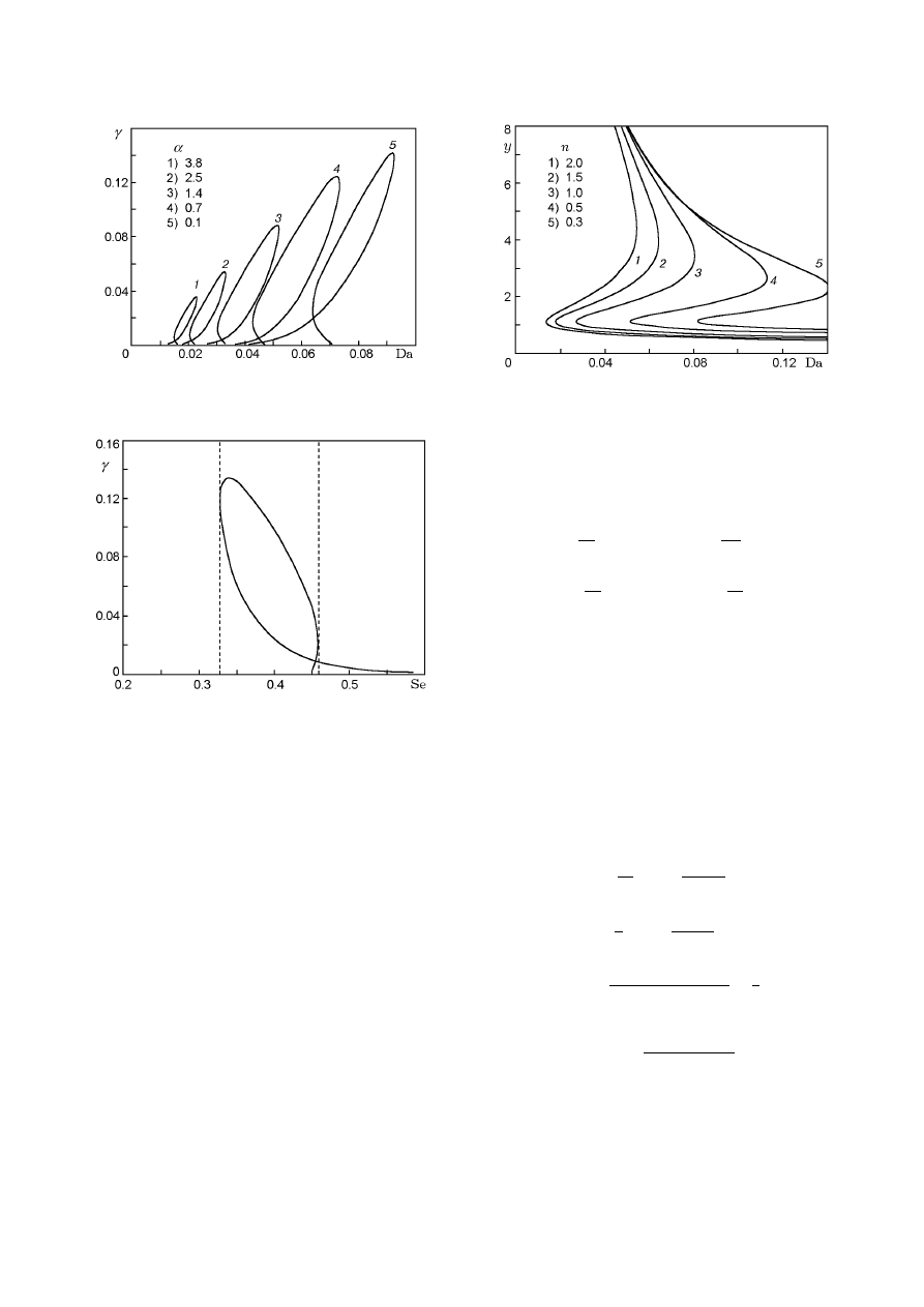
Varying the parameter α, which characterizes the

fuel-to-oxidizer ratio, one can study the variation of the
neutrality curve (Fig. 9). As in the case of the multiplic-
ity curves, explicit formulas of the type of (27) for the
remaining parameter planes become very cumbersome,
and we do not give them here. In this case, it is preferred

530

Bykov and Tsybenova

Fig. 9. Neutrality curves in the (Da, γ) plane for
β = 0.01 and Se = 0.45.

Fig. 10. Parametric portrait in the (Se, γ) plane for
Da = 0.05, β = 0.01, and α = 0.6.

to use a numerical procedure for constructing L

σ

based

on explicit formulas of the parametric dependences (21).

Parametric Portraits. A typical parametric por-

trait (curves L

∆

and L

σ

) is shown in Fig. 10, where L

∆

(region between the dashed lines) encloses the region
of three SS and L

σ

defines the change in the stability

of the SS (solid curve). The region of a unique unsta-
ble SS, which ensures the presence of self-oscillations in
system (17), is easily distinguished below the curve L

σ

and to the right of the second dashed line.

Thus, results of parametric analysis of model (17)

with variation of the fuel-to-oxidizer ratio show that sys-
tems with relatively small values of α (see Fig. 9) have
the largest region of existence of the critical conditions.
With increase in this ratio, the regions of existence of
multiple SS and self-oscillations decrease, i.e., an ex-
cess of oxygen, with other factors being equal, leads to
critical phenomena with higher probability.

Fig. 11. Steady-state temperature versus the param-
eter Da for β = 0.01 and Se = 0.4.

REACTION nA

→ P

For an nth-order reaction, the Zel’dovich– Semenov

model has the dimensionless form

dx

dt

= (1

− x)

n

e(y)

−

x

Da

,

(28)

γ

dy

dt

= (1

− x)

n

e(y)

−

y

Se

.

Steady States.

Steady states are determined

from the system

(1

− x)

n

e(y)

− x/Da = 0,

(29)

(1

− x)

n

e(y)

− y/Se = 0,

which is brought to the following form by the transfor-
mations described above:

(1

− νy)

n

e(y)

− y/Se = 0.

(30)

Parametric Dependences. We write the depen-

dences of SS on the parameters of the system that enter
into Eq. (30):

Da (y) =

Se

y

1

−

y

e(y)Se

1/n

,

ν(y) =

1

y

1

−

y

e(y)Se

1/n

,

(31)

β(y) =

1

ln(y/Se(1

− νy)

n

)

−

1

y

.

Assuming that ν = const, we express Se(y):

Se (y) =

y

(1

− νy)

n

e(y)

.

(32)

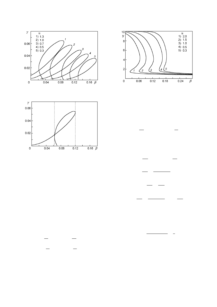
Figure 11 shows some dependences of steady-state tem-
perature on parameters, constructed with variation in

Parametric Analysis of the Simplest Model of the Zel’dovich–Semenov Model

531

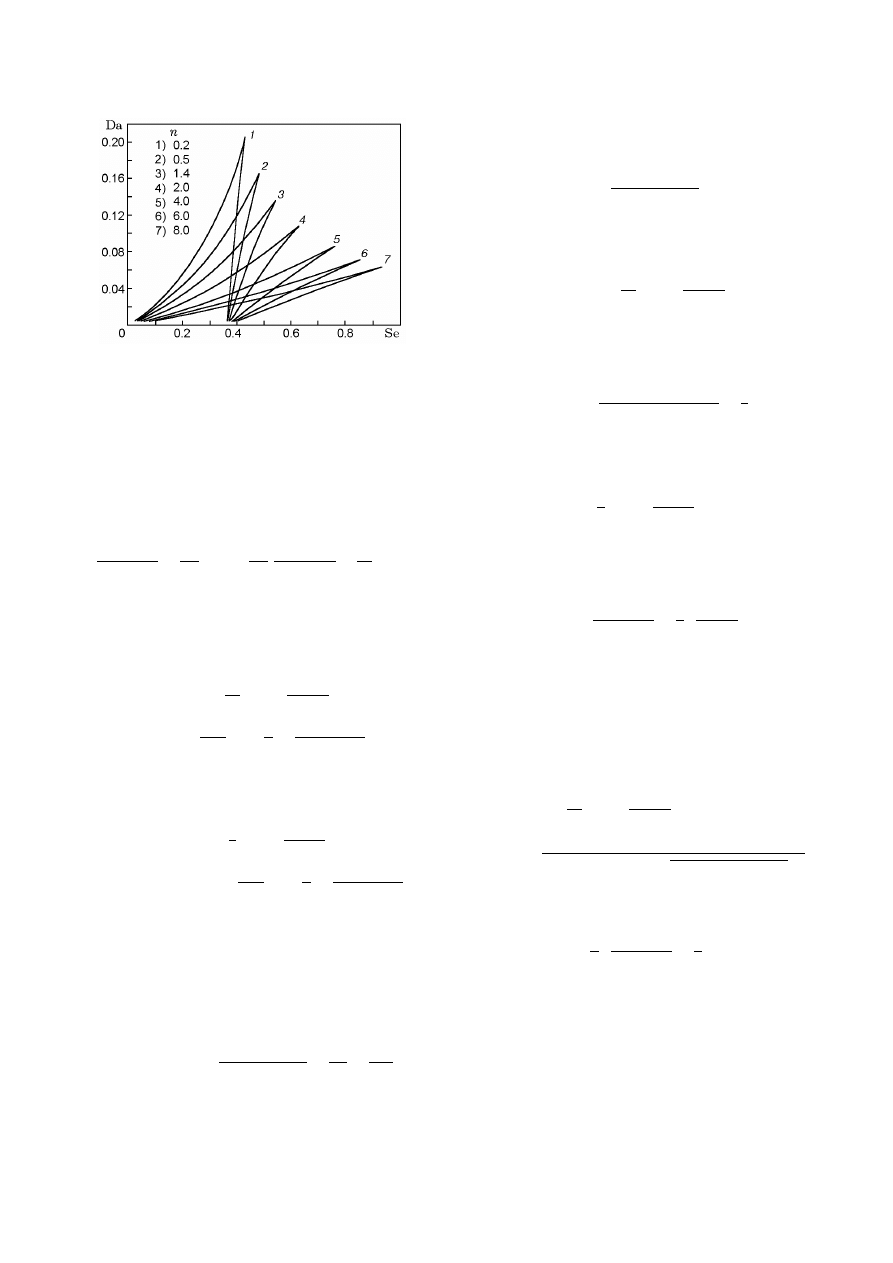
Fig. 12. Multiplicity curves in the (Se, Da) plane for
β = 0.

the reaction order n. One can see that the curves de-
pend strongly on n.

Multiplicity Curves.

The multiplicity condi-

tions for SS (curves L

∆

) are determined from the system

1

− Da/Se

y e(y) − y/Se = 0,

(33)

e(y)

(1 + βy)

2

−

Da

Se

e(y)

−

Da

Se

ye(y)

(1 + βy)

2

−

1

Se

= 0.

From (33), we obtain the following expressions for the
multiplicity curves in various parameter planes:

L

∆

(Da, Se):















Da (y, Se) =

Se

y

1

−

y

e(y)Se

1/n

,

Se (y) =

y

e(y)

1

−

1

n

+

y

n(1 + βy)

2

n

,

(34)

L

∆

(Se, ν):















ν(y) =

1

y

1

−

y

e(y)Se

1/n

,

Se (y) =

y

e(y)

1

−

1

n

+

y

n(1 + βy)

2

.

Figure 12 shows some dependences (34) obtained by
varying a third parameter. Variation of n leads to sub-
stantial change of the region of multiple SS.

Neutrality Curves. The stability regions for SS

(curves L

σ

) are determined from the system

(1

− νy)

n

e(y)

− y/Se = 0,

(35)

−n(1 − νy)

n

−1

e(y) +

(1

− νy)

n

e(y)

γ(1 + βy)

2

−

1

Da

−

1

γSe

= 0.

For ν = const, we obtain explicit expressions for the
neutrality curves:

L

σ

(γ, Se):







Se(y) =

y

(1

− νy)

n

e(y)

,

γ = γ(y, Se);

L

σ

(γ, Da):











Da (y) =

Se

y

1

−

y

e(y)Se

1/n

,

γ = γ(y, Da);

L

σ

(γ, β):











β(y) =

1

ln(y/Se (1

− νy)

n

)

−

1

y

,

γ = γ(y, β);

(36)

L

σ

(γ, ν):











ν(y) =

1

y

1

−

y

e(y)Se

1/n

,

γ = γ(y, ν).

Here

γ(y) =

1

(1 + βy)

2

−

1

y

1

− νy

n

.

Substituting Da(y, Se) into the second equation of

system (35), we arrive at the criticality condition in the
(Da, Se) plane:

L

σ

(Da, Se):























Da (y, Se) =

Se

y

1

−

y

e(y)Se

1/n

,

Se (y) =

y(2b)

n

e(y)

b + n

− 1 ±

p(b + n − 1)

2

− 4bn

n

.

Here

b =

1

γ

1

(1 + βy)

2

−

1

y

.

Figure 13 shows some curves (36) obtained by vary-

ing a third parameter.

In addition to expressions (34) and (36), one can

obtain explicit expressions for L

∆

and L

σ

in the remain-

ing planes, for example, (n, γ), (n, Da), etc.

532

Bykov and Tsybenova

Fig. 13.

Neutrality curves in the (β, γ) plane for

Da = 0.05 and Se = 0.45.

Fig. 14. Parametric portrait in the (β, γ) plane for
Da = 0.05, Se = 0.45, and n = 0.9.

Parametric Portraits. Figure 14 shows a para-

metric portrait plotted with the use of the explicit ex-
pressions for the multiplicity and neutrality curves. For
the remaining combinations of the planes of dimen-
sionless parameters, the portraits are constructed with
the use of the explicit expressions (34) and (36) or the
above-described graphical and numerical procedures of
the parameter-continuation method [8, 11].

REACTION A

→ P

WITH ARBITRARY KINETICS

For arbitrary kinetics, the dimensionless model has

the form

dx

dt

= f (x)e(y)

−

x

Da

,

(37)

γ

dy

dt

= f (x)e(y)

−

y

Se

,

where f (x) is an arbitrary kinetic function.

For ex-

ample, for an oxidation reaction of the general form

Fig. 15. Steady-state temperature versus the param-
eter β for Da = 0.05, Se = 0.5, and α = 0.2.

nA + mO

2

→ P, we have

f (x) = (1

− x)

n

(1

− αx)

m

.

Steady States. The steady states are determined

from the system

f (x)e(y)

−

x

Da

= 0,

f (x)e(y)

−

y

Se

= 0.

(38)

The equation for SS has the form

f (νy)e(y)

− y/Se = 0.

(39)

Jacobi Matrix Elements:

a

11

=

∂f

1

∂x

= f

0

(x)e(y)

−

1

Da

,

a

12

=

∂f

1

∂y

=

e(y)

γ(1 + βy)

2

f (x),

(40)

a

21

=

∂f

2

∂x

=

e(y)

γ

f

0

(x),

a

22

=

∂f

2

∂y

=

e(y)

γ(1 + βy)

2

f (x)

−

1

γSe

.

Here f

0

(x) = df /dx. Expressions (40) are calculated for

the SS in accordance with (39) and the equality x = νy.

Parametric Dependences. Using Eq. (39), we

express the SS as a function of β for an arbitrary kinetic
function f (x):

β(y) =

1

ln(y/Se f (x))

−

1

y

.

(41)

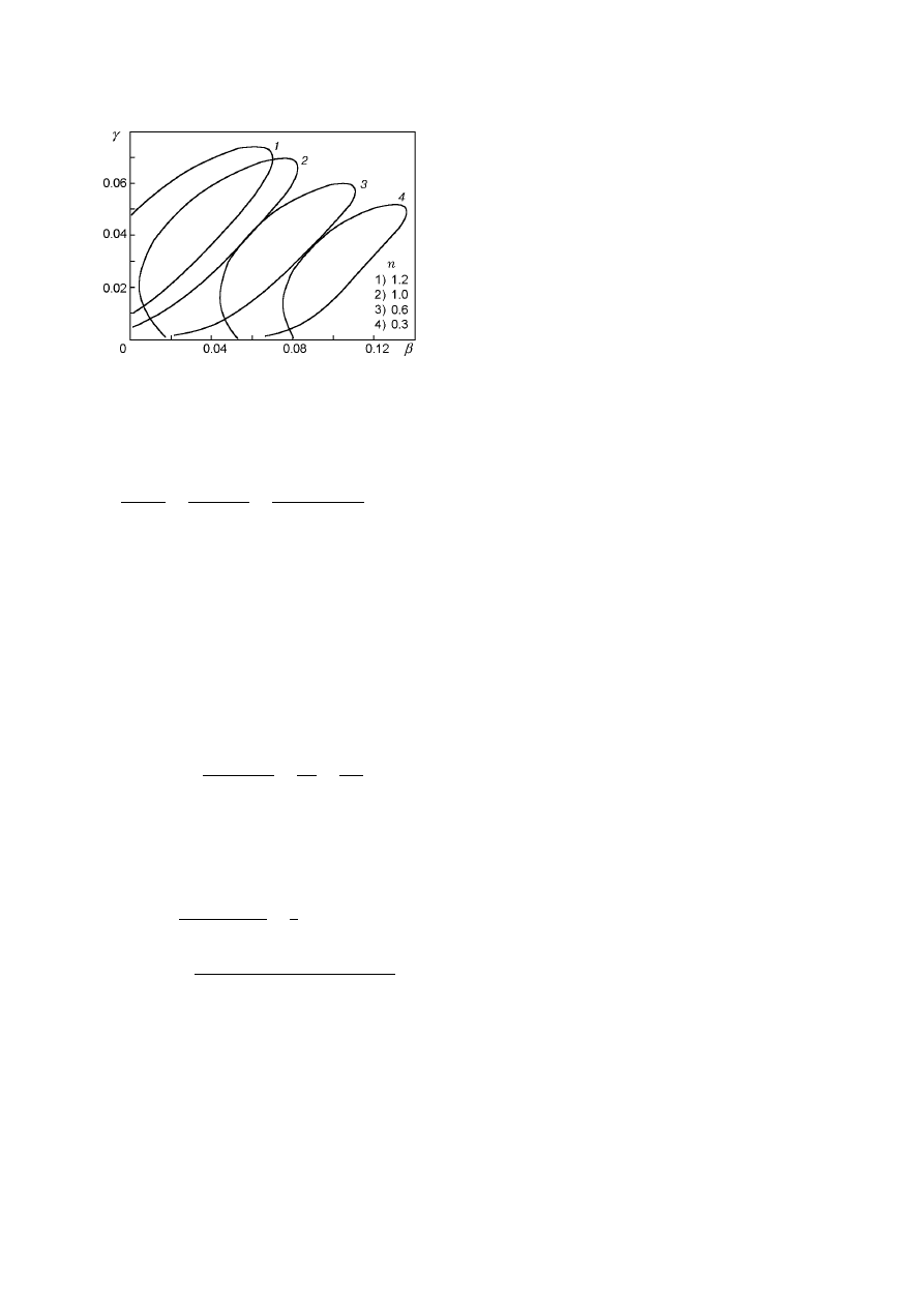
Figure 15 shows steady-state temperature versus the
parameter β for an nth-order oxidation reaction (nA +
O

2

→ P).

Multiplicity Curves. The curve of change in the

number of SS is given by

Parametric Analysis of the Simplest Model of the Zel’dovich–Semenov Model

533

Fig. 16.

Neutrality curves in the (β, γ) plane for

Da = 0.05, Se = 0.45, and α = 0.5.

f (x)e(y)

− y/Se = 0,

(42)

1

γDaSe

−

e(y)f

0

(x)

γSe

−

e(y)f (x)

Daγ(1 + βy)

2

= 0.

In the (γ, β) plane, the multiplicity curves (L

∆

),

as before, are two parallel lines for any f (x).

Hav-

ing the explicit form (41) of the parametric dependence
β(y), one can use the graphical method to obtain the
multiplicity curves for other combinations of parameter
planes, for example, (β, Da), (β, Se), etc., including the
parameters that enter into the kinetic function f (x).

Neutrality Curves.

To obtain the neutrality

curve, one need to solve the system

f (x)e(y)

− y/Se = 0,

(43)

f

0

(x)e(y) +

e(y)f (x)

γ(1 + βy)

2

−

1

Da

−

1

γSe

= 0.

We insert β(y) into the second equation of system (43)
and express γ(y):

L

σ

(γ, β):



















β(y) =

1

ln(y/Se f (x))

−

1

y

,

γ(y, β) =

Da (e(y)Se f (x)

− (1 + βy)

2

)

Se(1 + βy)

2

(1

− Da e(y)f

0

(x))

.

(44)

Figure

16

shows

results

of

calculation

by

(44)

for

the

kinetic

function

f (x)

=

(1

− x)

n

(1

− αx).

In this case, too, one can em-

ploy the graphical method of constructing bifurcation
curves in other parameter planes using the explicit
expression for β(y).

CONCLUSIONS

Parametric

analysis

applied

to

the

classical

Zel’dovich–Semenov model allowed us to construct
curves of local bifurcations of SS in various combina-
tions of planes of dimensionless parameters and study
the effect of other parameters on these curves. The re-
sults obtained are of methodical significance, since they
adequately describe the special features of one of the
basic models of the theory of thermal explosion. More-
over, these results are useful from the practical view-
point. Having explicit expressions for bifurcation curves
in the planes of dimensionless parameters, one can plot
these curves in the planes of dimensional parameters
that correspond to the specific geometry and thermal
characteristics of the real exothermic processes occur-
ring in continuous stirred tank reactors.

In this paper, in addition to the first-order reac-

tion, we considered the oxidation reactions A + O

2

→ P

and nA + O

2

→ P and the nth-order reactions nA → P.

Bifurcation curves describing the change in the num-
ber of steady states and type of their stability were
constructed in the planes of dimensionless parameters
by analytical and numerical methods.

A numerical-

analytical method of parametric analysis was proposed
for an arbitrary kinetic function f (x).

A comparative analysis of the parametric portraits

constructed for various kinetic functions shows that the
type of kinetics affects substantially the critical con-
ditions of ignition, multiplicity of SS, and presence of
self-oscillations.

REFERENCES

1. A. G. Merzhanov and V. G. Abramov, “Thermal

regimes of exothermic processes in continuous stirred

tank reactors,” Preprint, Joint Institute of Chemical

Physics, Acad. of Sci. of the USSR, Chernogolovka

(1976).

2. A. Uppal, W. H. Ray, and A. B. Poore, “On the dynamic

behavior of continuous stirred tank reactors,” Chem.

Eng. Sci., 29, No. 4, 967–985 (1974).

3. A. Uppal, W. H. Ray, and A. B. Poore, “On the dynamic

behavior of continuous stirred tank reactors,” Chem.

Eng. Sci., 31, No. 2, 205–221 (1976).

4. D. A. Vaganov, N. G. Samoilenko, and V. G. Abramov,

“Periodic regimes of continuous stirred tank reactors,”

Chem. Eng. Sci., 33, No. 6, 1133–1140 (1978).

5. V. S. Sheplev and M. G. Slin’ko, “Periodic regimes in

a perfect-mixing continuous stirred tank reactor,” Dokl.

Ross. Akad. Nauk, 352, No. 6, 781–784 (1997).

534

Bykov and Tsybenova

6. V. S. Sheplev, S. A. Treskov, and E. P. Volokitin, “Dy-

namics of stirred tank reactor with first-order reaction,”

Chem. Eng. Sci., 53, No. 21, 3719–3728 (1998).

7. B. V. Vol’ter and I. E. Sal’nikov, Stability of Modes of

Operation of Chemical Reactors [in Russian], Khimiya,

Moscow (1981).

8. M. Holodniok et al., Metody Analyzy Nelinearnich Dy-

namickych Modelu, Praha (1989).

9. V. I. Bykov, E. P. Volokitin, and S. A. Trescov,

“Mathematical model of a continuous stirred tank re-

actor: Parametric analysis,” Sib. Zh. Indust. Mat., 1,

No. 1, 57–76 (1998).

10. V. I. Bykov, E. P. Volokitin, and S. A. Treskov, “Para-

metric analysis of the mathematical model of a non-

isothermal well-stirred reactor,” Fiz. Goreniya Vzryva,

33, No. 3, 61–69 (1997).

11. S. I. Fadeev, S. A. Pokrovskaya, A. Yu. Berezin, and

I. A. Gainova, Software Package “STEP” for Numer-

ical Analysis of Systems of Nonlinear Equations and

Autonomous Systems of General Form. Description of

“STEP” Using Examples from the Course “Engineering

Chemistry of Catalytic Processes” [in Russian], Novosib.

Univ., Novosibirsk (1998).

12. S. B. Tsybenova, “Analysis of mathematical models of

processes in a nonisothermal continuous stirred reac-

tor,” in: Abstracts of Third Sib. Congr. on Applied and

Industrial Mathematics (INPRIM-98), Part 4, Novosi-

birsk (1998), pp. 78–79.

13. S. B. Tsybenova, “Parametric analysis of mathemati-

cal models for a nonisothermal continuous stirred re-

actor,” in: Mathematical Modeling in Natural Sciences,

Abstracts of All-Russ. Conf., Perm’ (1998), p. 79.

14. S. B. Tsybenova, “Mathematical modeling of the nitra-

tion dynamics of hydrocarbons in a continuous stirred

reactor,” in: Mathematical Models and Methods of Their

Analysis, Abstracts of Int. Conf., Krasnoyarsk (1999),

p. 205.

15. V. I. Bykov and S. B. Tsybenova, “Parametric analysis

of some basic models of combustion theory,” in: Chem-

ical Physics of Combustion (collected scientific papers

dedicated to 70th Anniversary of Acad. G. I. Ksandop-

ulo) [in Russian], Almaty (1999), pp. 133–135.

16. D. A. Frank-Kamenetskii, Diffusion and Heat Trans-

fer in Chemical Kinetics [in Russian], Nauka, Moscow

(1987).