Sukumar Supersymmetric quantum mechanics and its

Supersymmetric quantum mechanics and its

applications

C.V. Sukumar

Wadham College, University of Oxford, Oxford OX1 3PN, England

Abstract. The Hamiltonian in Supersymmetric Quantum Mechanics is defined in terms of charges
that obey the same algebra as that of the generators of supersymmetry in field theory. The conse-
quences of this symmetry for the spectra of the component parts that constitute the supersymmetric
system are explored. The implications of supersymmetry for the solutions of the Schrödinger equa-
tion, the Dirac equation, the inverse scattering theory and the multi-soliton solutions of the KdV
equation are examined. Applications to scattering problems in Nuclear Physics with specific refer-
ence to singular potentials which arise from considerations of supersymmetry will be discussed.

1. SUPERSYMMETRIC QUANTUM MECHANICS OF

ONE-DIMENSIONAL SYSTEMS

It is shown that every one-dimensional quantum mechanical Hamiltonian H can have
a partner ˜

H such that H and ˜

H taken together may be viewed as the components of

a supersymmetric Hamiltonian H. The term ‘supersymmetric Hamiltonian’ is taken to
mean a Hamiltonian defined in terms of charges that obey the same algebra as that of
the generators of supersymmetry in field theory. The consequences of this symmetry for
the spectra of H and ˜

H are explored. It is shown how the supersymmetric pairing may

be used to eliminate the ground state of H, or add a state below the ground state of H or
maintain the spectrum of H. It is also explicitly demonstrated that the supersymmetric
pairing may be used to generate a class of anharmonic potentials with exactly specified
spectra.

1.1. Introduction

In field theory, supersymmetry is a symmetry that generates transformations between

bosons and fermions. Unlike the generators of other symmetries whose algebra involves
commutators, the generators of the supersymmetric transformations are spinor charges
whose algebra involves anticommutators. Supersymmetry has raised the possibility of
providing a framework for a unified description of bosons and fermions which are
combined in the same supersymmetric multiplet [1]. Supersymmetric field theories may
be constructed by defining a superfield in a superspace, a space consisting of the usual
spacetime and in addition the anticommuting spinors of Grassmann [2]. The superfield

is a function of the spacetime coordinates x and also

and ¯

where

is an odd member

of the Grassmann algebra and ¯

is its conjugate. The supersymmetric transformation

may be viewed as a Grassmann even translation in this superspace. The generators of
this transformation are the supercharges.

There is a well defined procedure for starting from a field theory to construct a single

particle Quantum Mechanics and vice versa. For example Quantum Mechanics in one
dimension is defined by the Hamiltonian H = p

+ V (x) and the commutation relation

[x, p] = i¯h. The corresponding field theory starts by defining a space-time and the field

(x,t) is defined in this space-time by the Lagrangian L = [(

∂

)

−V (

)] and the action

S =

Ldt. It is well known that d = 1 quantum mechanics is formally equivalent to the

d = 1 quantum field theory with the identification x →

, p →

∂

and canonical quanti-

zation of the field

leads to the usual commutation relations between x and p. Similarly,

by constructing a Lagrangian invariant under the supersymmetric transformation, i.e. by
generalizing the d = 1 field to the superfield defined in superspace and integrating out
the Grassmann coordinates associated with the superspace, a Lagrangian expressed in
terms of the component fields of the superfield may be obtained. Canonical quantization
then leads to a Hamiltonian for Supersymmetric Quantum Mechanics. Witten [3] was
the first to construct a simple example of a supersymmetric system corresponding to
a spin−

1
2

particle moving in one dimension. Witten also defined the algebra that must

be satisfied by the charge operators in terms of which the supersymmetric Hamiltonian
may be expressed. These algebraic relations that Witten first formulated have now be-
come the defining relations of Supersymmetric Quantum Mechanics or SUSYQM in
abbreviation.

The word ‘supersymmetry’ was originally used to denote a symmetry built into cer-

tain field theories that permits transformations between component fields whose intrin-
sic spins differ by

1
2

¯h. However, by extracting a single particle Quantum Mechanics

from the field theory by integration of the Grassmann variables all reference to spin
is lost. What remains is an underlying symmetry of the Schrödinger differential equa-
tions for two related Hamiltonians. In fact, already in the 19th century a symmetry of
second-order differential equations had been identified by Darboux [4]. The Darboux
transformation relates the solutions of a pair of closely linked second order differential
equations (Schrödinger [5], Infeld and Hull [6]). Throughout these lectures the term ‘su-
persymmetric system’ will be used to describe systems governed by an underlying alge-
bra which is identical to, or derivable from, the algebra of supersymmetry in field theory
even if the systems under consideration have nothing to do with bosons and fermions as
they are commonly understood. This algebra is the algebra explicitly defined by Witten.

The study of the relationship between spectra, conservation laws and the existence of

operators that commute with the Hamiltonian has a long history. It is well known that the
conservation of energy, linear momentum and angular momentum arise when space-time
is homogeneous and isotropic which in turn lead to invariance of the Hamiltonian under
time translation, spatial translation and rotation. The invariance of the supersymmetric
Hamiltonian under translations in superspace is related to the existence of supercharges
that commute with the SUSY Hamiltonian and leads to definite relations between the
spectra of the bosonic and fermionic sectors. Just as in field theory supersymmetry
leads to specific relations between the component sectors of a supermultiplet, so also
in SUSYQM the existence of a generating operator that commutes with the Hamiltonian
leads to certain specific relations between the spectra and the eigenfunctions of the
component parts of the supersymmetric Hamiltonian. The links between the solutions

of two differential equations connected by the Darboux transformation are identical to
those arising from considerations of supersymmetry.

Witten’s seminal idea has now been developed into the subject of Supersymmetric

Quantum Mechanics: the study of quantum mechanical systems governed by an algebra
identical to that of supersymmetry in field theory. A number of people have played
an important role in the development of the subject. It will not be possible in these
lectures to do full justice to all the people who have contributed to this subject. I would
like to keep a chronological order of how the ideas have developed and refer to the
papers that act as markers in this progression. Witten’s 1981 paper was followed by other
examples of spin systems in magnetic fields and other such special systems that exhibited
an underlying supersymmetry ([7]-[14]). Bernstein and Brown [15] showed that by
exploiting the degeneracy between the ‘bosonic’ and ‘fermionic’ sectors of certain
one-dimensional Hamiltonians, the properties of the first excited state of the ‘bosonic’
component may be inferred from a knowledge of the ground state of the ‘fermionic’
component. It was then shown by Andrianov, Borisov and Ioffe [16] and Sukumar
[17, 18] that all one-dimensional systems can have supersymmetric partners. Andrianov,
Borisov and Ioffe [19] also showed that a simple extension of supersymmetric quantum
mechanics to arbitrary dimensions is possible.

The plan of the lectures is to cover topics in the following order. In the first lecture the

defining algebra of Supersymmetric Quantum Mechanics, the implications of this alge-
bra for the spectra of the component parts of the SUSY Hamiltonian, the factorization
of the Schrödinger equation, the procedure for the elimination of the ground state of a
Hamiltonian, the procedure for the introduction of a new bound state below the ground
state of a given Hamiltonian and the procedure for generating a new Hamiltonian with
unaltered spectrum will be discusssed using examples. Thus the first lecture will mainly
be concerned with showing that the existence of a SUSY partner to one-dimensional
Hamiltonians implies a hierarchy of Hamiltonians with a special relationship between
the eigenvalues and eigenfunctions of the different members of the hierarchy.

In the second lecture the radial Schrödinger equation will be studied. The implica-

tions of a SUSY partner to the radial Schrödinger equation will be used to differentiate
between four types of SUSY transformations. In the first part of the third lecture the un-
derlying supersymmetry of the Dirac equation for the Hydrogen atom will be discussed.
In the second part of the third lecture the supersymmetry linking the N and the N + 1
soliton solutions of the KdV equation will be discussed. The connection between the dif-
ferent types of supersymmetric transformations of the radial Schrödinger equation and
the approach of the conventional inverse scattering theory will be more fully explored
in the fourth and fifth lectures. It will be shown how certain choices of pairs of SUSY
transformations lead to the results of the conventional inverse scattering theory based
on the Gelfand-Levitan and Marchenko equations. It will be shown that other choices
of pairs of SUSY transformations lead to new results not present in the standard inverse
scattering theory and produce singular potentials which have found a variety of applica-
tions in Nuclear Physics. The fourth lecture will be concerned with the study of different
pairs of supersymmetric transformations and the different potentials that can be gener-
ated by this procedure. In the fifth lecture the procedures discussed in the earlier lectures
will be generalized and some applications of the new aspects of inverse scattering the-
ory arising from the singular potentials constructed using SUSY transformations of the

radial Schrödinger equation will be discussed.

Throughout these lectures units in which ¯h = 1 and the mass m = 1 will be used.

1.2. Supersymmetric quantum mechanics

SUSYQM is characterized by the existence of charge operators Q

that obey the

algebra

, Q

} =

i j

H ,

i, j = 1, 2, . . . , N ,

(1)

, H] = 0 ,

(2)

where H is the supersymmetric Hamiltonian, N is the number of generators and {, }
denotes an anticommutator. Here we consider the simplest of such systems with two
operators Q

and Q

. In terms of Q = (Q

+ iQ

√

2 and its Hermitian adjoint Q

†

− iQ

√

2 the algebra governing this supersymmetric system is characterized by

H = {Q, Q

†

} ,

= 0 ,

†2

= 0 .

(3)

From these equations it is clear that

[Q, H] = 0 ,

†

, H] = 0 .

(4)

i.e., the charge operator Q is nilpotent and commutes with the Hamiltonian H. A simple
realization of the algebra defined in Eq. (3) can be achieved by considering

Q =

−

†

0 A

(5)

where A

−

is an operator and A

is its adjoint. It is clear that with this construction Q

= 0

automatically. Eqs. (3) and (5) lead to the supersymmetric Hamiltonian

H =

−

(6)

Since

−

†

(7)

we can say that the operators Q and Q

†

induce transformations between the ‘bosonic’

sector represented by

and the ‘fermionic’ sector represented by

. We may also

interpret H in the following way: the scalar Hamiltonian H = A

−

has a partner ˜

H =

−

such that H and ˜

H are the diagonal elements of a supersymmetric Hamiltonian

H. Having demonstrated that a Q and an H can be constructed, we can switch to the
operator language of Quantum Mechanics to find out what the consequences of the
existence of a charge operator that commutes with the Hamiltonian are for the spectra
of the two sectors H and ˜

H. A

−

and A

−

are both positive semi-definite operators

with eigenvalues greater than or equal to 0. Let

be a normalized eigenstate of H with

eigenvalue E. Then

−

= E

(8)

Multiplication from the left by A

−

leads to

−

) = E(A

−

) .

(9)

If A

−

6= 0, we can infer that E is also an eigenvalue of A

−

. The corresponding

normalized eigenfunction ˜

of ˜

H can be shown to be given by

√

−

) .

(10)

The same reasoning may be applied starting from the eigenvalue equation for ˜

H instead

of H to investigate whether every eigenvalue of ˜

H is also an eigenvalue of H. If ˜

E is an

eigenvalue of ˜

H with eigenfunction ˜

−

= ˜

E ˜

(11)

then

−

) = ˜

E(A

) .

(12)

Therefore, if A

6= 0 then ˜

E is also an eigenvalue of H with the corresponding

normalized eigenfunction

√

) .

(13)

In view of the above relationships, three possibilities may be distinguished from each
other.

(a) If there is a normalizable eigenstate of H such that A

−

(0)

= 0, then A

−

(0)

= 0

and

(0)

corresponds to the ground state with eigenvalue E

(0)

= 0. Conversely, for the

eigenvalue E

(0)

= 0 the vanishing expectation value of A

−

in the ground state implies

that A

−

(0)

= 0. Under these circumstances, ˜

H has no normalizable eigenstate with

E = 0, i.e. there can be no normalizable state with A

= 0. The ground state eigenvalue

of ˜

H is non-zero. All eigenvalues other than the ground state eigenvalue of H are also

eigenvalues of ˜

H and all eigenvalues of ˜

H are also eigenvalues of H. The resulting

spectral mapping is shown in Fig. 1(a).

(b) If there is a normalizable eigenstate of ˜

H such that A

(0)

= 0, then A

−

(0)

0 and ˜

(0)

corresponds to the ground state of A

−

with eigenvalue ˜

(0)

= 0. There

cannot be a normalizable state of A

−

with eigenvalue zero that satisfies A

−

= 0.

The ground state of H has non-zero eigenvalue. All eigenvalues other than the ground
state of ˜

H are also eigenvalues of H and all eigenvalues of H are eigenvalues of ˜

H. This

leads to the spectral mapping shown in Fig. 1(b).

H such that either A

−

= 0 or

= 0, then the spectra of both H and ˜

H begin at positive values. Every eigenvalue

of H is also an eigenvalue of ˜

H and vice versa. The resulting spectral mapping is shown

in Fig. 1(c).

FIGURE 1.

Schematic diagram of the possible allignment of eigenvalues of the operators H

= H =

−

and H

= ˜

H = A

−

In each of the three cases the eigenfunctions of H and ˜

H for a common eigenvalue E

are linked in the manner indicated below:

(E) = exp(i

) (E)

−

1
2

−

(E) ,

(E) = exp(−i

) (E)

−

1
2

(E) ,

(14)

in which

is an arbitrary phase whose significance will become clear in later discussion.

The ladder structure of the eigenvalue spectrum shown in Fig. 1 and the intertwining
relationships between the eigenfunctions given above are characteristic hallmarks of
supersymmetric systems in one dimension and serve as signatures by which the presence
of an underlying supersymmetry may be inferred. In the early works on SUSYQM
([12, 15]) operators of the form

+U(x)

(15)

were considered in which U (x) was considered to be a known function of x. This
assumption restricts the applicability of SUSYQM to a limited class of problems. In
the next section it will be shown that it is not necessary to make any assumptions about

U and that U itself may be generated from the solutions of the Schrödinger equation

in one dimension. Such a generalization extends the applicability of SUSYQM to all
one-dimensional problems which have a ground state.

1.3. Factorization of the Schrödinger equation

The Schrödinger equation in one dimension is governed by the Hamiltonian

H = −

+V (x) ,

(16)

where V is the potential. H can be factorized in the form

H = A

−

√

(17)

where

is an undetermined constant, provided that the unknown function U satisfies

= 2(V −

) .

(18)

This is a nonlinear equation with a family of solutions. One member of the family is
given by

U =

(x,

)

(x,

) ,

(19)

where

(x,

) is a solution of the Schrödinger equation at energy E =

, i.e.

(x,

) =

εψ

(x,

) .

(20)

Since

−

(21)

it is easy to verify that Eq. (19) satisfies Eq. (18). It is clear that this argument is valid
only if

(x,

) is non-vanishing i.e.

(x,

) is nodeless. It can be shown that the general

solution to Eq. (18) is given by the one-parameter family of solutions

U (x,

) =

(x,

) +

(x,

)

dz/

(z,

)

(22)

where

is an arbitrary parameter. Every choice of

and the corresponding

(x,

)

leads to a possible factorization of H in the form H = A

(

−

(

) +

. The choice of

factorization energy

and the selection of a value for

must clearly be motivated by

the particular circumstances of a given problem and by physical considerations. If we
consider a Hamiltonian with a ground state energy E

(0)

, then the requirement that A

−

be a positive definite operator can be met only if the energy

is chosen to be

≤ E

(0)

We consider the case when the factorization energy

= E

(0)

next.

1.4. Factorization energy

equals the ground state energy E

(0)

With the choice of E

(0)

as the factorization energy, the ground state eigenfunction

(x, E

(0)

) is nodeless and vanishes in the asymptotic region. The requirement that U(x)

in Eq. (22) should not be divergent leads to the choice

∞

, giving

U (x) =

(x, E

(0)

) ,

(0)

) =

√

(x, E

(0)

)

= A

(0)

−

(0)

) + E

(0)

(23)

It is clear that A

−

has a spectrum beginning at 0, with a ground state which satisfies

−

(0)

= 0 with

(0)

(x, E

(0)

). The analysis in §1.3 can now be used by considering

the partner Hamiltonian

H = E

(0)

+ A

−

(0)

) = H + [A

−

(0)

), A

(0)

)] ,

(24)

corresponding to the potential

V (x) = V (x) −

(0)

(25)

H and ˜

H have their spectra aligned as in Fig. 1(a). ˜

H has no eigenstate corresponding to

the ground state of H and all the excited states of H are degenerate with the eigenstates
of ˜

H. The eigenfunctions of the two Hamiltonians are linked in the form

(x, E) = (E − E

(0)

)

−

1
2

−

(0)

)

(x, E) ,

(x, E) = (E − E

(0)

)

−

1
2

(0)

) ˜

(x, E) ,

(26)

by choosing the phase

in Eq. (14) to be zero. These equations are valid not only when

E is one of the discrete eigenvalues of H , E = E

( j)

( j 6= 0), but also when E lies in the

continuous part of the spectrum. When E lies in the continuous part of the spectrum
of H the above equations can be used to find a relation between the transmission
coefficients in the potentials V (x) and ˜

V (x) at energy E since the asymptotic form of

the wavefunction for potential V at energy E implies a definite asymptotic form for the
wavefunction for ˜

V at the same energy. This procedure will be illustrated by considering

the phase shift for the solutions of the radial Schrödinger equation in the second lecture.
Since the above anlysis is valid for any one-dimensional Hamiltonian H

with the ground

state with energy E

(0)

and wave function

(0)

the process of finding a supersymmetric

partner can be iterated to generate the hierarchy of Hamiltonians given by

(x) = −

(x) ≡ A

−

+ E

(0)

= A

−
n−1

+
n−1

+ E

(0)

n−1

n = 2, 3, . . . ,

(27)

where

(x) =

√

(0)

(x)

n = 1, 2, . . . ,

(x) = V

n−1

(x) −

(0)

n−1

(x) ,

n = 2, 3, . . . ,

(28)

in which E

( j)

and

( j)

are the eigenenergies and eigenfunctions of H

with the property

that

(m)

= E

(m+1)

n−1

= . . . = E

(m+n−1)

(m)

= [E

(m)

− E

(0)

n−1

]

−

1
2

−
n−1

(m+1)

n−1

(m+1)

n−1

= [E

(m)

− E

(0)

n−1

]

−

1
2

+
n−1

(m)

n = 2, 3, . . . ,

m = 0, 1, 2, . . . . (29)

FIGURE 2.

Schematic diagram of the eigenvalue spectra of the Hamiltonians in the hierarchy H

. The

number of bound states of H

is arbitrarily chosen to be 5.

A pictorial representation of the eigenvalue correspondence of the Hamiltonian hierar-
chy is given in Fig. 2.

The equations given above show that the excited states of V

can be obtained from the

ground states of the hierarchy V

. The simple harmonic oscillator, the particle in a box,

the radial equation for a definite partial wave for the Coulomb potential and the Morse
potential are all examples where the potentials corresponding to the Hamiltonians in the
hierarchy can be analytically worked out [17]. One nontrivial example of such an exactly
solvable hierarchy will be discussed next.

1.5. Attractive sech

potential

Let

= −

sech

x ,

> 0 .

(30)

Since this potential is attractive in all space −

∞

≤ x ≤

∞

it will support atleast one bound

state irrespective of the strength of the potential. In terms of the parameter

1
2

≥

(31)

the spectrum of this potential is given by [20]

(m)

= −

−

m +

¶¸

m = 0, 1, 2, . . . , N ≤ Q

−

(32)

The potential in Eq. (30) supports a finite number (N + 1) of bound states. The ground
state wavefunction

(0)

(x) ∼ sech

−

1
2

)

x ,

(33)

leads to

(x) = −

− Q

sech

x .

(34)

Inspection of this equation shows that

(i) if

> 1, then V

(x) is an attractive sech

x potential;

(ii) if

= 1, then V

(x) vanishes and H

is a free particle Hamiltonian;

(iii) if

< 1, then V

(x) is a repulsive potential and corresponds to a sech

x barrier.

It is easy to show that the parameter correspoding to Q

for V

+ 2

− Q

¶¸

1
2

= Q

− 1 .

(35)

The spectrum of H

is then given by

(m)

= −

−

m +

¶¸

(36)

which satisfies the condition E

(m)

= E

(m+1)

. Iteration of this argument shows that the

Hamiltonian hierarchy corresponds to a sequence of shape-invariant potentials with
successively decreasing strengths. It is easy to show that

(x) = −

sech

x ,

1
2

= Q

n−1

− 1 .

(37)

If N = Q

−

1
2

then V

N+1

(x) vanishes. If N < Q

−

1
2

< N + 1 then V

N+2

corresponds to

a sech

barrier given by

N+2

(x) =

− N −

¶ µ

N +

− Q

sech

x .

(38)

We have shown that by choosing the factorization energy

to be the ground state

energy it is possible to generate a new Hamiltonian H

without an eigenstate corre-

sponding to the ground state of H

but retaining the rest of the spectrum of H

. It has

been demonstrated that this procedure may be iterated to generate a Hamiltonian hierar-
chy with spectra aligned as in Fig. 2. In the next subsection we examine other possible
factorizations.

1.6. Factorization energy

less than the ground state energy

When the factorization energy

in Eq. (17) is less than the ground state energy of

H the solution

(x,

) of H

εψ

is not a normalizable solution eventhough

(

)

is still a solution of A

−

(

) = 0. The lack of normalizability of

(

) means that

(

−

(

) cannot have zero as an eigenvalue and the spectrum of A

−

begins

at positive values. The analysis in §1.3 shows that when A

−

has no normalizable

eigenstate with eigenvalue zero, it is possible for A

−

to have a spectrum beginning

at eigenvalue zero. For A

−

to have a normalizable state with eigenvalue zero, the

solution ˜

of A

(

) ˜

= 0 must be normalizable. The solution of

(x,

)

(x,

) = 0 ,

(39)

i.e.

(x,

) =

(x,

)

(40)

shows that if the unnormalizable solution

(x,

) of the Hamiltonian H is chosen in

such a way that (

)

−1

is normalizable, then ˜

(x,

) is normalizable and A

−

has a

spectrum beginning at eigenvalue zero. Therefore

H = A

−

(

) +

< E

(0)

(41)

has a ground state at energy ˜

(0)

with a ground state eigenfunction ˜

(0)

(x,

) = ˜

(x,

Therefore, ˜

H has a ground state eigenvalue below the ground state of H while all the

other eigenvalues of ˜

H are degenerate with the eigenvalues of H. This corresponds to

the level scheme shown in Fig. 1(b). Hence when (

)

−1

is normalizable

H = H −

[ln

(x,

)] ,

(42)

has ground state

(0)

< E

(0)

(x,

) =

(x,

)

(43)

and excited states with

(m+1)

= E

(m)

m = 0, 1, 2, . . . ,

(m+1)

= −

(m)

−

1
2

−

(m)

= −

(m)

−

1
2

(m+1)

(

) =

√

(x,

)

(44)

The phase factor

in Eq. (14) has been chosen to be

. Having chosen

to be zero

for the case of elimination of a state in §1.5, the requirement that adding a state by a
transformation and subsequently eliminating the same state by another transformation
should give back the original transformation, fixes the phase factor for the case of
the addition of a state to be

. If

< E

(0)

, but the unnormalizable solution

(x,

)

does not lead to a normalizable (

)

−1

and the second derivative of ln

(x,

) is well

behaved, in a sense to be defined shortly, then neither A

(

−

(

) nor A

−

(

)

has a normalizable eigenstate with eigenvalue zero. We denote such a solution

Therefore A

−

and A

−

have identical spectra as depicted in Fig. 1(c). Then

H = A

−

(

) +

= H −

(x,

) ,

(45)

has a spectrum identical to that of H. The relations between the eigenvalues and the
eigenstates are given by

(m)

= E

(m)

m = 0, 1, 2, . . . ,

(m)

= exp(i

)

(m)

−

1
2

−

(m)

= exp(−i

)

(m)

−

1
2

(m)

(

) =

√

(x,

)

(46)

The phase factor

has been left undetermined. Furthermore, the non-normalizable

solutions

and ˜

for energy

are connected by

(x,

) =

(x,

)

(47)

In this section we assume that −

∞

≤ x ≤

∞

and postpone the discusion of 0 ≤ r ≤

∞

a later section. It is necessary to make this distinction because the type of singularities
of the potential V that are physically admissible depends on the range of values of the
variable x. Potentials with singularities of the form r

−2

are admissible for the radial

problem, but singularities of the form x

−2

are inadmissible when −

∞

≤ x ≤

∞

. The

discussion of the construction of a normalizable

−1

depends on the spatial domain in

which

and V are defined. We now examine the question of the normalizability of

−1

when −

∞

≤ x ≤

∞

. Let

(x,

) be a nodeless solution of H

εψ

for

< E

(0)

. The

existence of such a solution can be rigorously proved [21]. Another linearly independent
solution at the same energy is given by

(x,

) =

(x,

)

(z)

(48)

The nodelessness of

guarantees that this integral is well defined. The general solution

at the energy

is given by

(x,

) =

αφ

1 +

−

∞

(49)

in which the lower limit of the integral has been chosen to be −

∞

and

is an arbitrary

constant. Let

(

) =

∞

−

∞

(z,

)

−1

(50)

It can be shown that for values of

in the range −

∞

will remain nodeless

and

is unnormalizable. It can also be shown that for −

∞

−1

is singularity

free and normalizable. This range of values of

then leads to a normalizable

−1

and

−1

corresponds to an eigenstate of ˜

H as defined in Eq. (42) with ground state

eigenvalue E

(0)

. It can be shown that for the limiting values

= −

and

∞

even though

−1

is unnormalizable the second derivative of ln

is divergence free and

finite in the asymptotic region. These values of

then lead to ˜

H defined in Eq. (45)

with the same spectrum as H. But if

< −

then

will vanish for some finite value of

x as can be seen from Eq. (49) and the second derivative of ln

(x,

) then diverges

when

vanishes. Hence for

< −

(x,

) does not lead to a physically acceptable

potential ˜

V . The above analysis will be illustrated with examples in the next section.

1.7. Free particle, addition of bound state

Let V (x) = 0. H has only a positive energy spectrum. For negative energies

−

/2, the general solution of H

εψ

is given by

(x,

) = cosh

x +

sinh

x .

(51)

Though

is unnormalizable, for values of the parameter

in the range |

| < 1

nodeless and

−1

is normalizable. The family of potentials

V = V −

(x,

) = −

(1 −

)

(cosh

x +

sinh

| < 1 ,

(52)

therefore have a single bound state at energy

(0)

= −

(53)

with ground state eigenfunction

(0)

∼

cosh

x +

sinh

| < 1 .

(54)

For positive energies, Eq. (46) then gives

(x,

) = −

2(E − ˜

(0)

)

−

1
2

−

sinh

x +

cosh

x +

sinh

(x, E) .

(55)

In the asymptotic region |x| →

∞

, this equation becomes

lim

|x|→

∞

(x, E) = −

2(E − ˜

(0)

)

−

1
2

−

lim

|x|→

∞

(x, E) .

(56)

The

independence of this equation means that the transmission coefficient of this

family of potentials V (x, E,

) are identical. This family of potentials is an example of

the phase-equivalent family of Bargmann [22].

1.8. Simple harmonic oscillator, addition of bound state

The oscillator potential does not belong to the category of potentials that remain finite

in the asymptotic region. Nevertheless, the oscillator example serves to clarify some of
the discussion in the text. The harmonic oscillator Hamiltonian

H = −

(57)

has the eigenvalue spectrum

E = (n +

) ,

n = 0, 1, 2, . . . .

(58)

The even solution of H

εψ

for all energies can be written in series form [23] and is

given by

(x,

) =

1 +

(4 +

)

(4 +

)(8 +

)

+ . . .

−x

(59)

where

= 1 − 2

(60)

For energies below the ground state of the oscillator

< E

(0)

1
2

> 0, which

guarantees that

is positive definite. Thus

is a nodeless unnormalizable solution

for

1
2

. The linearly independent solution

(x,

) =

(z)

(61)

can also be written in series form as

(x,

) =

1 + (

+ 2)

+ (

+ 2)(

+ 6)

+ . . .

−x

(62)

vanishes at x = 0 but the series within the parentheses is positive definite when

1
2

Both

and

may be expressed in terms of standard parabolic cylinder functions. The

general solution at energy

is then given by

(x,

) =

(x,

) +

αφ

(x,

) .

(63)

In terms of the parameter

lim

x→

∞

(

) =

∞

(z,

)

−1

= 2

(

3
4

−

1
2

)

(

1
4

−

1
2

)

(64)

which arises from asymptotic formulae for the parabolic cylinder functions [23], for
|

| <

(x,

) =

(x,

)

1 +

(z,

)

(65)

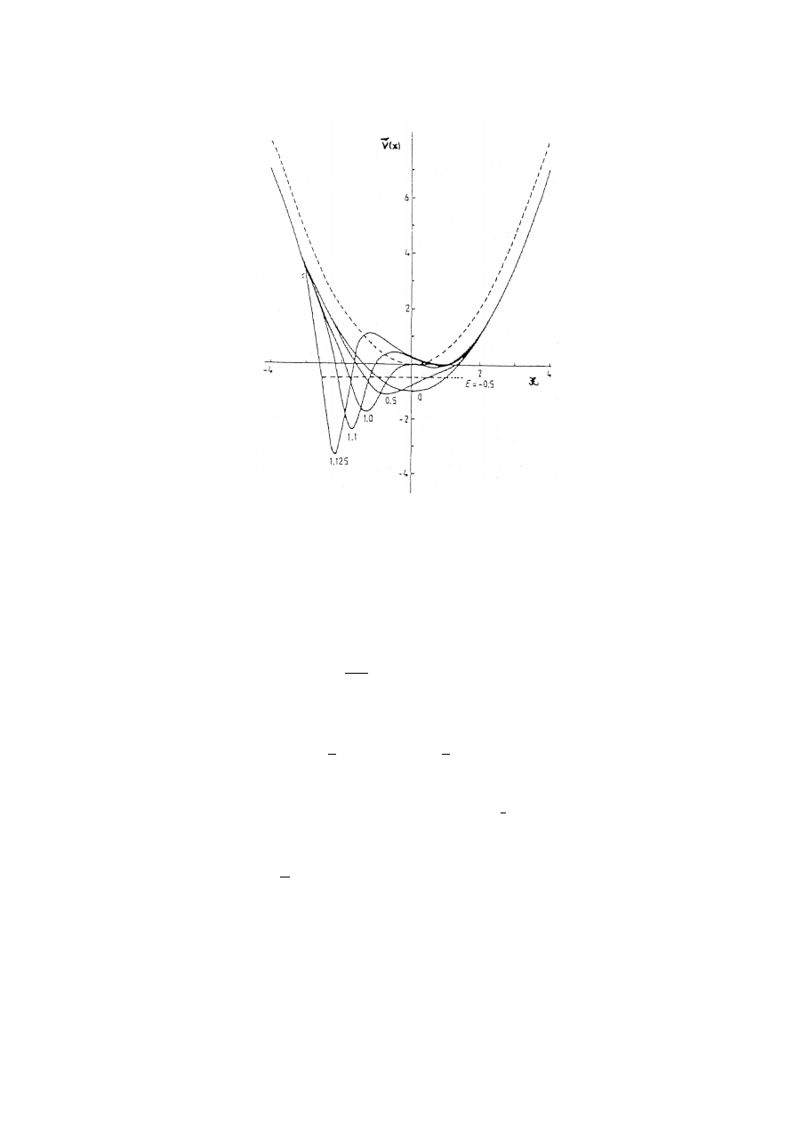
FIGURE 3.

The phase-equivalent potentials ˜

V (x,

) are shown for

= −1/2. The value of

indicated below each curve. The harmonic oscillator potential V (x) = x

/2 is also shown as a broken

curve. The potentials shown in figure by full curves have identical spectra with ground state at ˜

(0)

= −1/2

as indicated by the horizontal broken line. The rest of the spectrum is identical to that of the harmonic
oscillator.

is nodeless and

−1

is normalizable. The family of Hamiltonians

H = H −

(x,

) ,

| <

(66)

therefore have identical spectra given by

(0)

(m)

= m −

m = 1, 2, . . . .

(67)

This family of potentials is another example of the phase-equivalent family of Bargmann
[22]. Since the energy ˜

(0)

is arbitrary as long as ˜

(0)

1
2

, the above equations give a

recipe for constructing anharmonic potentials with spectra defined by Eq. (67).

Using the series expansion for

and

the potentials ˜

V (x,

) have been calculated

for a range of values of

and

(

). Fig. 3 shows ˜

V for

= −1/2 and

in the range

of values 0 <

< 2/

√

. The results for positive values of

are shown. The potential

for the corresponding negative value of

may be obtained by mirror reflection about

the x-axis. For

= 0, ˜

V (x) = x

/2 − 1 is a shifted oscillator. This is the only value of

for which ˜

V is invariant under the parity transformation. Thus by imposing a specific

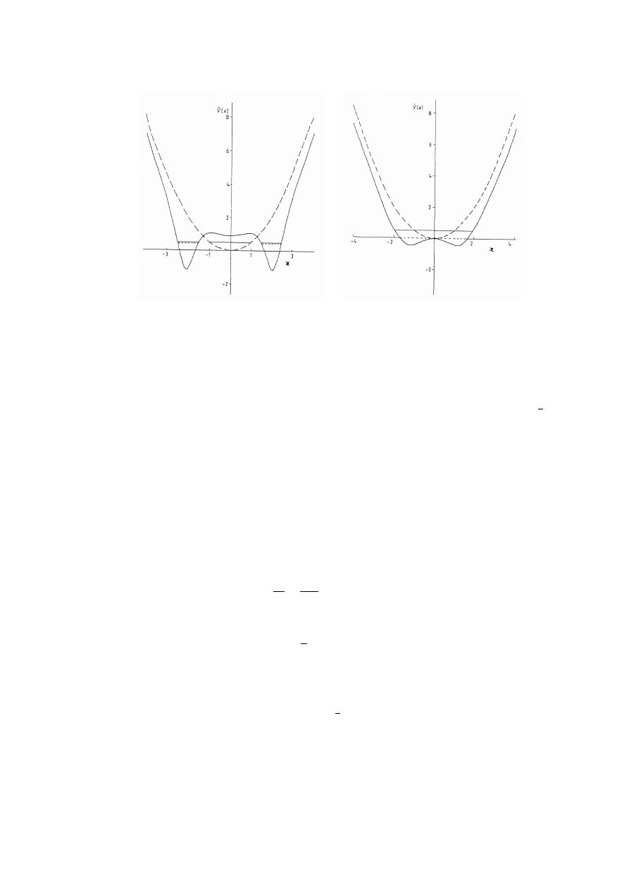
(a)

(b)

FIGURE 4.

The potential ˜

V (x,

) for

= 0 and (a)

= 0.45, (b)

= 0.0, The harmonic oscillator

potential is indicated as a broken curve. The ground state of V at E = 0.5 is indicated by a full horizontal
line and the ground state of ˜

V at E =

is indicated by a broken horizontal line. The rest of the spectrum

of ˜

V is identical to that of the harmonic oscillator.

condition on ˜

V (x) a unique member of the family is obtained. Fig. 4 shows ˜

V (x,

, 0) for

a range of values of

for a fixed value of

= 0. These figures show that for 0 <

1
2

the ground state of the new potential ˜

V lies inside the double well. This is an example

of the general result that when

lies below the ground state of a given potential V , but

> V

min

(x) where V

min

is the minimum of the potential, the resulting partner potential

V (x) is necessarily a double well. It can be shown on general grounds that a double well

is necessary to accomodate the new level at

close to the first excited state of ˜

V (x) at

energy E

(0)

. Fig. 4 shows double well potentials whose spectrum is fixed by construction

to be of the form given in Eq. (67).

We next consider the limiting values

(

) for which

(x,

)

−1

is unnormaliz-

able. The value of

for a given value of

may be found from Eq. (64). It can be shown

that the second derivative of ln

is divergence free. Hence

V (

) =

−

(x,

, ±

(

)) ,

(68)

has the spectrum

(m)

= m +

m = 0, 1, 2, . . . ,

(69)

which is identical to the spectrum of the harmonic oscillator. The eigenfunctions of

H may be given in terms of the oscillator eigenfunctions using the intertwining rela-
tions involving the A

operators using the logarithmic derivative of

(x,

(

)). Thus

Hamiltonians ˜

) for various values of

1
2

which have spectra identical to the har-

monic oscillator may be constructed. The potentials ˜

V (x,

(

)) have been calculated

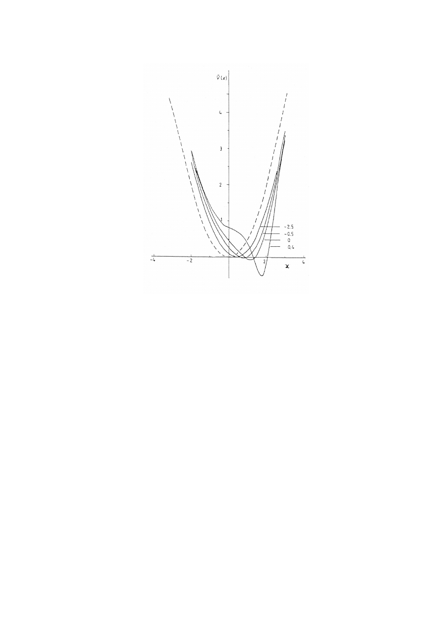
FIGURE 5.

The potential ˜

V (x,

(

)) for a range of values of

. The

value is indicated on each

curve. The harmonic oscillator potential is shown as a broken curve. All the potentials shown in this
diagram have spectra identical to that of the harmonic oscillator. The asymptotic values of the full curves
are given by lim

x→

∞

∆

V = −1, lim

x→−

∞

∆

V = +1 where

∆

V = ˜

V (x) −V (x).

numerically and are shown in Fig. 5 for a range of values of

and positive values of

(

). The potentials for negative

may be obtained by mirror reflection.

1.9. Summary

It has been demonstrated that the algebra of supersymmetry can be used to find partner

Hamiltonians to one-dimensional Hamiltonians. The flexibility in the choice of the part-
ner Hamiltonian enables the identification of different types of supersymmetric pairings.
A procedure for constructing Hamiltonians with either identical spectra or with identical
spectra apart from a missing ground state has been given. This procedure has been illus-
trated with several examples. This recipe can be used to either add a new ground state
eigenvalue to, or eliminate the ground state of or maintain the same spectrum of a given
Hamiltonian corresponding to a Schrödinger equation. This procedure may be repeated
again and again in a suitable combination to generate hierarchies of Hamiltonians whose
spectra are related to each other. By applying this procedure to the harmonic oscillator

anharmonic potentials whose spectra are identical to that of the harmonic oscillator or
contain a ground state lower in eigenvalue than the ground state of the harmonic oscil-
lator have been constructed.

2. SUSYQM AND INVERSE SCATTERING THEORY

The radial Schrödinger equation corresponding to a definite partial wave is studied.
The procedures for finding a new potential by eliminating the ground state of a given
potential by adding a bound state below the ground state of a given potential and by
generating the phase-equivalent family of a given potential using the supersymmetric
pairing of the spectra of the operators A

−

and A

−

are examined. Four different

types of transformations generated by the concept of a supersymmetric partner to a given
radial Schrödinger equation are identified and the modifications of the Jost functions for
the four transformations are classified. It is argued that the Bargmann class of potentials
may be generated using suitable combinations of the four types of transformations.

2.1. Introduction

In the first lecture (§1) it was shown that by using the idea of a supersymmetric partner

to a Hamiltonian function H of a single variable it is possible to find another Hamiltonian

H which had one of the following features: either (i) the complete spectrum of ˜

H is made

up of all the eigenvalues of H except the ground state of H , or (ii) the complete spectrum
of ˜

H is made up of all the eigenvalues of H and in addition one further eigenvalue which

lies below the ground state of H, or (iii) the spectrum of ˜

H is identical to that of H.

It was shown that in all three cases the eigenfunctions of H and ˜

H for the common

eigenvalues are connected by a linear differential operator. By repeated application of
this procedure of either deleting an eigenvalue or adding an eigenvalue or maintaining
the same eigenvalues it is possible to generate Hamiltonians whose spectra bear a
definite relationship to each other. The inverse scattering theory can also accomplish
the same tasks through solving either the Gelfand-Levitan [24] or the Marchenko [25]
equations [13, 26, 27]. The aim of this lecture is to elucidate the relationship between
the two approaches [28]. It will also be shown that the Bargmann class of potentials [22]
may be genearted by the application of the concept of supersymmetric pairing.

The radial Schrödinger equation differs from the Schrödinger equation in the space

[−

∞

] in essential respects. The boundary conditions on the eigenfunctions and the

allowed singularities of the potential are different in the two spaces [−

∞

] and [0,

∞

In this lecture the modifications introduced by switching from x to r will be considered
first and then the modifications of the Jost function corresponding to four different types
of transformations will be studied.

2.2. The radial Schrödinger equation

We now consider the radial Schrödinger equation for a definite partial wave with the

Hamiltonian

= −

+V (r) ,

V (r) =

l(l + 1)

+ v(r) .

(70)

The potential V (r) is assumed to be regular, not singular. Specifically, the potentials
discussed here are restricted to be no more singular than r

−2

at the origin and decreasing

at least as fast as r

−2

as r →

∞

In this lecture the term ‘normalization constant of the eigenfunction’ will be used

often. This term has a specific meaning in the terminology of the inverse scattering
theory. All bound state eigenfunctions are understood to be normalized to unity in the
usual way to reflect the condition that the total probability of finding the bound particle
somewhere in space should be unity. However, in the inverse scattering method the term
‘normalization constant’ is used in a specific sense. The regular solution

of the radial

Schrödinger equation is defined to be a solution that satisfies the boundary condition

lim

r→0

(r, E, l) =

l+1

(2l + 1)!!

(71)

The regular solution will grow exponentially as r →

∞

when E is not one of the eigenen-

ergies. However, when E is one of the eigenenergies E

(i)

the bound state eigenfunction,

which decreases exponentially as r →

∞

, is proportional to the regular solution

(r, E

(i)

, l) =

αφ

(r, E

(i)

, l) ,

∞

dr = 1 .

(72)

It is this proportionality constant

that corresponds to the ‘normalization constant’

referred to in the inverse scattering method. Throughout this lecture the term ‘normal-
ization constant’ will be used in the sense in which it is used in the inverse scattering
theory. The term ‘normalizable’ will, however, be used in the usual sense of the word,
i.e.,

∞

dr is finite. In view of the different types of transformations of the radial equa-

tion that will be discussed the following notations will be adopted. The eigenfunctions
of H defined in Eq. (70) are denoted by

(i)

for the discrete states at energies E

(i)

, the

phase shifts for the continuum states

(r, E) for positive energies E =

1
2

are denoted

(l, k) and the Jost function by F(l, k). The potentials, eigenstates, phase shifts and

Jost function after the supersymmetric transformation are denoted by adding a tilde,

(r, E), for example. The different types of transformations are distinguished by adding

a suffix, ˜

(r, E), for example. We adopt the notation that

(m)

(r) is an abbreviation for

(r, E

(m)

2.3. Jost function

In scattering theory the S-matrix may be constructed from the Jost function [29]. The

integral representation of the Jost function for a potential v(r) with N bound states at
energies E = E

(i)

and phase shifts

(l, k) at energies E =

1
2

for angular momentum l

is given by (see Chadan and Sabatier [30], for example)

F(l, k) =

∏

i=1

1 −

(i)

exp

−

∞

(l, p)pd p

− k

(73)

The phase of the Jost function is −

(l, k) while the modulus is given by

|F(l, k)| =

∏

i=1

1 −

(i)

exp

−

∞

(l, p)pd p

− k

(74)

where the symbol P stands for principal value. The spectral density for positive energies
is given by

dP(E)

(l+

1
2

)

|F(l, k)|

−2

(75)

Knowledge of the phase shifts for all positive energies, the bound state energies E

(i)

and

the normalization constants C

(i)

associated with each of the bound states enables the

complete determination of the potential V (r).

2.4. Elimination of the ground state

By the methods discussed in §1 it can be shown that H defined by Eq. (70) has a

supersymmetric partner

= H −

(0)

(r) .

(76)

Since

lim

r→0

(r) ∼ r

l+1

(77)

corresponds to the potential

(r) =

(l + 1)(l + 2)

+ v(r) −

(0)

(r)

l+1

(78)

where the singularity at the origin has been separated to show the behaviour near the
origin. It can be established that

lim

r→0

(r) =

(l + 1)(l + 2)

lim

r→

∞

(r) =

l(l + 1)

(79)

has no normalizable state with eigenvalue E

(0)

and therefore the ground state of V is

missing from the spectrum of eigen values for ˜

. All the other eigenvalues of the two

potentials are the same. The eigenfunctions are related by

(m)

= (E

(m)

− E

(0)

)

−

1
2

−
1

(m)

m = 1, 2, . . . ,

−
1

√

−

(0)

(r)

(80)

Extension of the above eigenfunction relation to positive energy states and use of the
asymptotic forms

lim

r→

∞

(r, E) ∼ sin

kr −

(l, k)

lim

r→

∞

(0)

(r) ∼ exp(−

(0)

r) ,

(81)

then gives

lim

r→

∞

(r, E) ∼ sin

kr −

+ ˜

(l, k)

(82)

where

(l, k) =

(l, k) −

− tan

−1

(0)

E =

(0)

(83)

The phase shift relation is consistent with the observation that when r → 0 the singularity
of the potential ˜

corresponds to l → l + 1 which implies an increased repulsion and

therefore the phase shift should decrease. In the limit k → 0 the phase shift decreases by

which is the correct limit when a bound state has been eliminated. In the limit k →

∞

the phase shift decreases by

/2. Eqs. (73), (74), (80) and (83) enable the establishment

of a relationship between the Jost functions for the potentials ˜

and V . The phase

shift relation given in Eq.(83) may be used to compare the Jost functions for the two
potentials. Using the integral relation [31]

∞

cot

−1

(p/

)

− k

pd p = ln

1 +

(84)

we can establish that the Jost functions for the two potentials are related by

(l, k)

F(l, k)

k − i

(0)

(85)

2.5. Addition of a bound state

The potential ˜

with a ground state at ˜

E = −

1
2

< E

(0)

, i.e., below the ground state

of V in addition to sharing all the eigenvalues of V can be constructed by the methods

of §1. Since the potential in the radial equation can have singularities of the form r

−2

the equations of §1 must be recast in an appropriate form. The regular solution in the
potential V at energy E denoted by

satisfies

lim

r→0

l+1

(2l + 1)!!

lim

r→

∞

∼ exp( ˜

r) .

(86)

Since the energy E is below the ground state of V ,

is nodeless for r > 0 and may be

chosen to be positive definite for r > 0. The linearly independent solution can be taken
to be

(r) =

(r)

∞

(z)

(87)

It is easy to show that

lim

r→0

(r) ∼ r

−l

lim

r→

∞

(r) ∼ exp(− ˜

r) .

(88)

The function

is one of the Jost solutions (see [29], for example) defined by a boundary

condition in the asymptotic region. For energies ˜

E < E

(0)

is also a nodeless function

and is positive definite. When ˜

E is not only less than E

(0)

but also less than the absolute

mimimium of the potential V then the positivity of (V − ˜

E) guarantees that

and

are monotonically growing functions of r in the directions r = 0 →

∞

and r =

∞

→ 0,

respectively. When V

min

< ˜

E < E

(0)

and

are no longer monotonically growing

functions but nevertheless remain nodeless. These assertions on the behaviour of

and

may be rigorously proved. The function

cos

sin

(89)

is also a nodeless function when 0 <

1
2

and

−1

is a normalizable function for this

range of values of

since

lim

r→0

= lim

r→0

sin

∼ r

(90)

and

lim

r→

∞

= lim

r→

∞

cos

∼ exp(− ˜

r) .

(91)

By the methods of §1 it is easy to infer that when 0 <

1
2

(r) = V (r) −

(r, ˜

) ,

(92)

with

(r, ˜

) =

(r, ˜

cos

+ sin

∞

(z, ˜

(93)

has a ground state at

(0)

= ˜

E ,

(94)

with eigenfunction

(0)

(r, ˜

) =

(r, ˜

)

(95)

All the other eigenvalues of ˜

are identical to the eigenvalues of V . The other eigen-

functions of ˜

are given by

(m)

= −(E

(m)

− ˜

−

1
2

−
2

(m)

m = 1, 2, . . . ,

−
2

( ˜

) =

√

−

(r, ˜

)

(96)

The potential ˜

may be written in the form

(r, ˜

) =

l(l − 1)

+ v(r) −

ln(r

(r, ˜

)) ,

(97)

where the singularity at the origin has been separated to show the behaviour near the
origin. It can be established that

lim

r→0

l(l − 1)

lim

r→

∞

l(l + 1)

(98)

Extension of Eq. (96) to positive energy states and use of the asymptotic forms

lim

r→

∞

(r, E) ∼ sin

kr −

(l, k)

lim

r→

∞

(r, ˜

) ∼ exp( ˜

r) ,

(99)

then gives

lim

r→

∞

(r, ˜

) ∼ sin

kr −

+ ˜

(l, k)

(100)

where

(l, k) =

(l, k) +

+ tan

−1

(101)

The phase shift relation is consistent with the observation that when r → 0 the singularity
of the potential ˜

corresponds to l → l − 1, which implies a decrease in the repulsion

and therefore the phase shift should increase. In the limit k → 0 the phase shift increases
by

which is the correct limit when the number of bound states increases by one. In the

limit k →

∞

the phase shift increases by

/2. The equations given above show that all

members of the family ˜

(r, ˜

) lead to identical phase shifts for the same energy E

when 0 <

1
2

. Furthermore, since

lim

r→0

(r, ˜

) = −

(102)

Eq.(96) shows that for a fixed principal quantum number m, lim

r→0

(r, ˜

) is inde-

pendent of

and therefore the excited states of ˜

(r, ˜

) for various

have identical

normalizations. However, the normalized ground state eigenfunction

(0)

(r, ˜

) =

(sin

cos

)

1
2

(cos

+ sin

∞

dz/

(z))

∞

(0)

dr = 1 ,

(103)

shows that

lim

r→0

(0)

(r, ˜

) ∼

sin

cos

1
2

(104)

Hence the ground state eigenfunction of the family of potentials ˜

(r, ˜

) have differ-

ent normalizations, i.e., different proportionalities to the regular solution, although they
belong to the same eigenvalue. It has been shown that the phase shifts, the eigenvalues
and the normalization constants of the excited states are identical for all members of the
family of potentials ˜

(r, ˜

), 0 <

1
2

, while the ground state eigenfunctions be-

longing to the eigenvalue ˜

(0)

= ˜

E have different normalization constants for different

values of

. Clearly the family ˜

(r, ˜

) is an example of the phase equivalent family

which was discussed by Bargmann [22].

The phase shifts and the bound state energies of V and ˜

enable the comparison of

the Jost functions. From Eqs. (73) and (102) it is easy to show that

(l, k)

F(l, k)

k − i ˜

(105)

2.6. Boundary values of

and equivalent potentials

When the parameter

lies outside the range 0 <

1
2

, the eigenfunction

Eq. (89) does not lead to a normalizable

−1

. When −

< 0 or

1
2

vanishes at some finite value of r because either sin

or cos

assumes negative values

and

∞

dz/

can take all values from 0 to

∞

. If

vanishes at a finite value of r then

the second derivative of ln

diverges at this point. This would then lead to a singular V .

However, the critical values

= 0 and

1
2

must be studied separately.

(a) When

= 0

(r, ˜

E, 0) =

lim

r→0

∼ r

l+1

lim

r→

∞

∼ exp( ˜

r) .

(106)

The vanishing value of

at r = 0 shows that

−1

is not normalizable, but

lim

r→0

∼ −

(l + 1)

lim

r→

∞

∼ 0 .

(107)

The positivity of

guarantees that there are no singularities in the second derivative

of ln

for r > 0. These conditions ensure that it is possible to find a non-singular

supersymmetric partner to V . It can be shown that

(r, ˜

E) =

(l + 1)(l + 2)

+ v(r) −

(r, ˜

l+1

(108)

and that

lim

r→0

(r, ˜

E) =

(l + 1)(l + 2)

lim

r→

∞

(r, ˜

E) =

l(l + 1)

(109)

The eigenvalue spectrum of ˜

is identical to that of V and the new eigenfunctions are

(m)

= (E

(m)

− ˜

−

1
2

−
3

(m)

−
3

( ˜

E) =

√

−

(r, ˜

(110)

The phase shifts in the potentials are related by

(l, k) =

(l, k) −

+ tan

−1

(111)

The phase shift relation is consistent with the observation that when r → 0 the singularity
of the potential ˜

corresponds to l → l + 1, which implies an increased repulsion and

therefore the phase shift should decrease. In the limit k →

∞

the phase shift decreases by

/2. In the limit k → 0 the phase shift is unchanged which is the correct limit since the

two potentials have the same number of bound states. The family of potentials ˜

(r, ˜

for different values of ˜

E < E

(0)

have identical spectra but different phase shifts for the

same energy. The Jost functions for the potentials V and ˜

can be shown to be related

in the manner

(l, k)

F(l, k)

k + i ˜

(112)

(b) When

1
2

(r, ˜

) =

lim

r→0

∼ r

−l

lim

r→

∞

∼ exp(− ˜

r) .

(113)

Hence

1
2

does not lead to a normalizable

−1

, because

−1

diverges as r →

∞

However,

lim

r→0

lim

r→

∞

∼ 0 .

(114)

These conditions together with the absence of any singularities in the second derivative
of ln

ensure that a singularity-free supersymmetric partner to V may be constructed. It

can be shown that

(r, ˜

E) =

l(l − 1)

+ v(r) −

(r, ˜

(115)

and that

lim

r→0

(r, ˜

E) =

l(l − 1)

lim

r→

∞

(r, ˜

E) =

l(l + 1)

(116)

The eigenvalue spectrum of ˜

is identical to that of V and the eigenfunctions are related

(m)

= −(E

(m)

− ˜

−

1
2

−
4

(m)

−
4

( ˜

E) =

√

−

(r, ˜

(117)

The phase shifts in the potentials are related by

(l, k) =

(l, k) +

− tan

−1

(118)

The phase shift relation is consistent with the observation that when r → 0 the singularity
of the potential ˜

corresponds to l → l − 1, which implies a decreased repulsion and

therefore the phase shift should increase. In the limit k →

∞

the phase shift increases by

/2. In the limit k → 0 the phase shift is unchanged which is the correct limit since the

two potentials have the same number of bound states. The family of potentials ˜

(r, ˜

for different values of ˜

E < E

(0)

have identical spectra but different phase shifts for the

same energy. The Jost functions for the potentials V and ˜

can be shown to be related

in the manner

(l, k)

F(l, k)

k + i ˜

(119)

2.7. Summary

It has been shown that by a suitable factorization of the radial Schrödinger equation, it

is possible to discover an underlying supersymmetric algebra. This algebra may be used
to generate four different types of transformations of the radial Schrödinger equation.
The four transformations may be classified as follows.

(1) T

is a transformation that eliminates the ground state [E

(0)

] of the potential

V (r), leaves the rest of the spectrum of eigenvalues unaltered, leaves the angular mo-

mentum component of the potential in the region r →

∞

unaltered and alters the singular

behaviour near r → 0 to a centrifugal potential corresponding to angular momentum
(l + 1). T

also changes the Jost function corresponding to V by a multiplicative factor

k/(k − i

(0)

) where

(0)

= [−2E

(0)

]

1
2

. The new eigenfunctions in the potential (78) are

given by Eq. (80).

(2) T

is a transformation that adds a bound state ˜

(0)

, ˜

(0)

below the ground state

of the potential V (r), leaves the rest of the spectrum of eigenvalues unaltered, leaves
the angular momentum component of the potential in the region r →

∞

unaltered and

alters the singular behaviour near r → 0 to a centrifugal potential corresponding to
angular momentum (l − 1). T

also changes the Jost function corresponding to V by

a multiplicative factor (k − i ˜

(0)

)/k where ˜

(0)

= [−2 ˜

(0)

]

1
2

. The new eigenfunctions in

the potential in Eqs. (92) and (93) are given by Eqs. (95) and (96).

(3) T

is a transformation that maintains the eigenvalue spectrum of V unaltered,

leaves the angular momentum component of the potential in the region r →

∞

unaltered

and alters the singular behaviour near r → 0 to a centrifugal potential corresponding to
angular momentum (l +1). T

also alters the Jost function for V by a multiplicative factor

k/(k + i ˜

) where ˜

= [−2 ˜

1
2

and ˜

E < E

(0)

. The new eigenfunctions in the potential

(108) are given by Eq. (110).

(4) T

is a transformation that maintains the eigenvalue spectrum of V unaltered,

leaves the angular momentum component of the potential in the region r →

∞

unaltered

and alters the singular behaviour near r → 0 to a centrifugal potential corresponding to
angular momentum (l −1). T

also alters the Jost function for V by a multiplicative factor

(k + i ˜

)/k where ˜

= [−2 ˜

1
2

and ˜

E < E

(0)

. The new eigenfunctions in the potential

(115) are given by Eq. (117).

In the one-dimensional case −

∞

< x <

∞

, the singularities in the potential at x = 0 are

not permitted and the physical eigenfunctions are defined by boundary conditions at ±

∞

In the case of the radial equation the boundary conditions on the eigenfunctions at r = 0
and r =

∞

are different. All four types of transformations listed above have analogues in

the space [−

∞

] but with the difference that no singularities of the type x

−2

should be

introduced by the transformations because of the boundary conditions usually imposed
on

(x). In the x space ˜

and ˜

arise from considering the limiting values

∞

and

= −

discussed in §1.6.

2.8. Relationship to Bargmann potentials

It has been shown above that each of the transformations T

− T

corresponds to

a multiplication of the Jost function by a specific rational function of k. By repeated
application of a combination of the four types of transformations in an appropriate order
the Jost function of V can be modified by any rational function of k. The generation of the
Bargmann class of potentials [7] corresponds to such a modification of the Jost function.
Therefore it is clear that the Bargmann class of potentials may be generated by a suitable
combination of T

, T

, and T

. For example, the multiplication of the Jost function by

a factor (k + ib)/(k + ia) can be broken down into two steps, multiplication by (k + ib)/k
followed by a further multiplication by k/(k + ia), corresponding to application of T

followed by T

. The physically acceptable Jost functions must satisfy the condition

lim

k→

∞

F(l, k) = 1 ,

(120)

and the symmetry relation

F(l, −k

) = [F(l, k)]

(121)

The modifications of F introduced by T

-T

clearly satisfies these conditions.

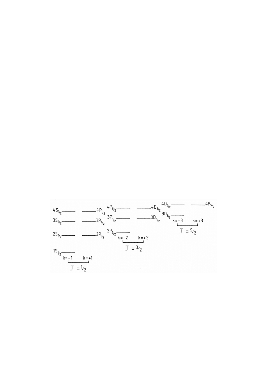
3. SUPERSYMMETRY AND THE DIRAC EQUATION FOR A

CENTRAL COULOMB FIELD

It is shown that the methods of Supersymmetric Quantum Mechanics can be used to
obtain the complete energy spectrum and eigenfunctions of the Dirac equation for an
attractive Coulomb potential.

3.1. The Dirac equation for the Coulomb potential

The Dirac equation for the electron in an attractive central Coulomb field leads to the

energy eigenvalue spectrum shown schematically in Fig. 6. The conventional spectro-
scopic classification of the levels in the non-relativistic limit is indicated alongside the
levels.

When the spectrum is unscrambled in this fashion, it is clear that the arrangement of

the pair of levels for a fixed value of the total spin J resembles a ‘supersymmetric’ pairing
in which the ‘fermionic’ ladder has a spectrum identical to the ‘bosonic’ ladder except
for the missing ground state. The level scheme in Fig. 6 corresponds to a juxtaposition
of one such ‘supersymmetric’ pair of ladders for each possible value of J. We now show
that the eigenvalue spectrum and the eigenfunctions of the Dirac equation may indeed
be obtained using the methods of SUSYQM.

Adopting the notation used in Bjorken and Drell [32] and defining the parameters

c¯h

= m + E ,

= m − E ,

(122)

FIGURE 6.

Schematic eigenvalue spectrum of the Dirac equation for the central Coulomb potential

V (r) = −

/r. J is the total spin and k = ±(J + 1/2). The quantum numbers are explained in the text.

the coupled radial equations satisfied by the two-component eigenfunction (G

, F

) may

be written in the matrix form

/dr

−

¶ µ

, (123)

in which k is an eigenvalue of the operator −(

· L + 1) with the allowed values

k = ±1, ±2, ±3, . . . and satisfies |k| = J + 1/2. In the representation in which Eq. (123)
is written, J and k are good quantum numbers. G

is the ‘large’ component in the non-

relativistic limit. The radial functions G

and F

must be multiplied by appropriate two-

component angular eigenfunctions to make up the full four-component solutions of the
Dirac equation. Fig. 6 shows that when we compare the two ladders of levels for a fixed
value of J, a pair of degenerate levels corresponds to the same value of J but opposite
values of k except for the lowest state of the pair of ladders when only the negative value
of k corresponds to an eigenstate. We now show how this ladder structure may be related
to the pairing of states characteristic of supersymmetric theories (Sukumar [33]).

The matrix multiplying 1/r in Eq. (123) may be diagonalized using the matrix D given

D =

k + s

−

k + s

s = (k

−

)

1/2

(124)

and its inverse. Mutiplication of the matrix differential equation from the left by D and
introduction of the new variable

= Er leads to

−

G ,

−

G =

−

F .

(125)

where

= D

(126)

These equations are similar to the relation between the two components of the eigen-
functions of a supersymmetric Hamiltonian

H = {Q , Q

†

} ,

Q =

−
0

†

0 A

+
0

(127)

and

±
0

−

(128)

The nilpotent operator Q commutes with H and therefore corresponds to a conserved
charge of this system. Q and Q

†

induce transformations between the ‘bosonic’ sector

represented by ˜

F and the ‘fermionic’ sector represented by ˜

G. Eq. (125) may be viewed

as a representation of such a transformation. In supersymmetric Quantum Mechanics the
‘fermionic’ and ‘bosonic’ components have identical spectra except for the ground state
of the ‘bosonic’ sector which is annihilated by the charge operator Q.

In other words the eigenvalue equations for ˜

F and ˜

+
0

−
0

+ 1 −

F ,

−
0

+
0

G =

+ 1 −

G ,

(129)

show that every eigenvalue of A

+
0

−
0

is also an eigenvalue of A

−
0

+
0

except when A

−
0

F =

0. The condition A

−
0

F = 0 leads to the ground state eigenfunction

(0)

exp(−

γρ

/s) ,

(130)

and the ground state energy eigenvalue is given by

(0)

= m

/(1 +

) .

(131)

−
0

+
0

has no normalizable eigenstate at this energy. All the other states of A

+
0

−
0

and

−
0

+
0

are paired and the eigenfunctions are linked in the form ˜

F ∼ A

+
0

G and ˜

G ∼ A

−
0

as indicated in Eq. (125). We now show how the ground state of A

−
0

+
0

may be obtained.

The uncoupled second order differential equations for ˜

F and ˜

−

s(s − 1)

+ 1 −

= 0 ,

(132)

−

s(s + 1)

+ 1 −

G = 0 ,

(133)

show that Eq. (133) may be obtained from Eq. (132) by the replacement s → s + 1. This
suggests that Eq. (133) may be written in the form

+
1

−
1

G =

(s + 1)

+ 1 −

G ,

(134)

with

±
1

s + 1

−

s + 1

(135)

G has a supersymmetric partner ˜

H which satisfies

−
1

+
1

H =

(s + 1)

+ 1 −

H .

(136)

Just as ˜

F and ˜

G may be viewed as the component eigenfunctions of a supersymmetric

Hamiltonian so also ˜

G and ˜

H may be viewed as the component eigenfunctions of another

supersymmetric Hamiltonian. The spectrum of ˜

H is identical with that of ˜

G except for

a missing state at the energy corresponding to the ground state eigenvalue of A

+
1

−
1

. By

the same reasoning as for A

+
0

−
0

we may then infer that the ground state of A

+
1

−
1

has

the eigenfunction

(0)

= exp[−

γρ

/(s + 1)] ,

(137)

with a ground state energy eigenvalue which satisfies

(0)

1 +

/(s + 1)

(138)

The excited states of A

+
1

−
1

satisfy equations similar to Eq. (125). Explicitly

s + 1

G = A

+
1

H ,

s + 1

−

= A

−
1

G .

(139)

Having obtained the ground state ˜

(0)

we can now use the supersymmetric pairing of ˜

and ˜

G to obtain the first excited state of A

+
0

−
0

in the form

(1)

∼ A

+
0

(0)

(1)

= E

(0)

(140)

where the suffixes carry obvious meaning.

This procedure may be repeated to find the ground state of a hierarchy of operators

+
2

−
2

, A

+
3

−
3

, . . . with each iteration corresponding to a shift of s by 1 in the definition of

the A

operators. This hierarchy corresponds to the Hamiltonian hierarchy discussed in

§1. From the ground state properties of the members of this hierarchy all the excited
state eigenfunctions and eigenvalues of A

+
0

−
0

can be obtained. The allowed energy

eigenvalues of Eq. (125) are

(n)

1 +

/(s + n)

n = 0, 1, 2, . . . ,

(141)

and the eigenfunctions may be written in the form

(n)

∼

+
0

+
1

. . . A

+
n−1

s+n

exp[−

γρ

/(s + n)] ,

(142)

with

= ±

s + n

−

s + n

(143)

Although ˜

F and ˜

G satisfy uncoupled second order differential equations, the normal-

ization of one of them determines that of the other as is required by Eq. (125). The
solution of Eq. (123) can be written, after adding the suffix n, in the form

(n)
k

(n)

2s(k + s)

k + s

¶ µ

(k/s − m/E)

−1

−
0

(n)

(144)

When n = 0, ˜

G has no normalizable eigenstate at energy E

(0)

. We treat the two

possible values of k for this energy separately. When k = −sm/E

(0)

Eq. (125) requires

that we must choose

F(−k,

) =

exp(−

γρ

/s) ,

G(−k,

) = 0 ,

(145)

to obtain normalizable solutions for F

and G

. However, when k = + sm/E

(0)

Eq. (125)

requires that we must choose

F(+k,

) =

exp(−

γρ

/s) ,

G(+k,

) =

−s

exp(+

γρ

/s)

exp(−2

x/s)dx .

(146)

Since ˜

G is not normalizable, the positive value of k does not lead to normalizable

solutions for F

and G

The expression for the spectrum, Eq. (141), is an even function of k. A fixed |k| leads

to a doublet of states corresponding to k = +|k| and k = −|k| degenerate in energy for all
positive integral values of n. For n = 0, only the negative value of k leads to normalizable
F

and G

and therefore the state with n = 0 is a singlet. This explains the ladder structure

of the spectrum for a fixed value of |k| = J + 1/2 and opposite values of k.

The above analysis considered a fixed k with the corresponding s = (k

−

)

1/2

However, in Eqs. (141)-(143) s enters only as a parameter. Hence we can obtain the
complete spectrum and the eigenfunctions of Eq. (123) for all values of J = |k| − 1/2 by
the above procedure. The complete spectrum is given by

(n)

1 +

n + (k

−

)

1/2

n = 0, 1, 2, . . . ,

k = 1, 2, . . . ,

(147)

and Eq. (142) for the eigenfunctions ˜

(n)

is valid for different values of s(k). The

principal quantum number N is related to n and k by the relation N = n + |k|.

We have shown that the supersymmetric pairing of ˜

F and ˜

G enables an elegant treat-

ment of the Dirac equation for a central Coulomb field (Darwin [34], Biedenharn [35]).
The interaction of a charged particle with the vacuum fluctuations of the quantized radi-
ation field leads to departures from the Coulomb potential. When the field deviates from
a Coulomb field, the transformed states ˜

F and ˜

G no longer belong to a supersymmetric

pair and the eigenvalue spectrum loses the ladder structure characteristic of supersym-
metric pairing. Therefore we may say that the Lamb shift, which is an effect due to
vacuum fluctuations, is related to the breaking of the supersymmetry that connects ˜

and ˜

4. SUPERSYMMETRY, POTENTIALS WITH BOUND STATES AT

ARBITRARY ENERGIES AND MULTI-SOLITON SOLUTIONS

OF KDV EQUATION

The connection between the algebra of supersymmetry and the inverse scattering method
can be used to construct reflectionless potentials with any specified number of non-
degenerate bound states at arbitrary energies. The reflection coefficient of the potential
so constructed is related to the reflection coefficient of a potential which supports no
bound states. By choosing the reference potential to be V = 0 it is possible to construct
reflectionless potentials with bound states at arbitrary energies. It is well known that
the KdV equation has muti-soliton solutions with known analytical form. The N-soliton
and the (N + 1)-soliton solutions of the KdV equation may be shown to be connected
by a transformation identical to that of the transformation linking the eigenfunctions of
the bosonic and fermionic sectors of a Supersymmetric pair. The reflectionless potential
with N bound states constructed using the ideas of the SUSY method to plant bound
states can be shown to be identical to the N-soliton solution of the KdV equation for
appropriate choice of a set of parameters.

4.1. Potentials with a single bound state

Let V

(x) be a potential that supports no bound states and R

(k) be the reflection

coefficient for positive energies. Using the procedure outlined in §1.7 ([18]) it is possible
to find a potential V

which supports a single bound state at energy E

= −

/2. It was

shown in §1.7 that V

may be written in the form

= V

−

) ,

(148)

where

) is a nodeless unnormalizable solution of the Schrödinger equation for the

potential V

at energy E

. It was shown in §1.7 that the ground state eigenfunction of V

at energy E

is given by

) ∼

)

(149)

while for E 6= E

(E) ∼ A

−
0

)

(E) ,

(150)

where

−
0

) =

√

−

)

(151)

The reflection coefficient of V

is given by

(k) =

− ik

+ ik

(k) .

(152)

The above results simplify for the case of a free particle for which V

= 0 and R

(k) = 0.

Eq. (152) shows that the reflection coefficient for the supersymmetric partner vanishes
identically. The non-normalizable solution in V

for energy E

is given by

) = cosh

x +

sinh

x ,

| < 1 .

(153)

The condition |

| < 1 ensures that

) is a nodeless function even though it is not

normalizable. The reflectionless potential V

with a single bound state at E

is given by

= −

sech

x + tanh

−1

(154)

with the ground state eigenfunction

) ∼ sech

x + tanh

−1

(155)

When

= 0, V

is a symmetric reflectionless potential. Using the suffix SR to denote

‘symmetric and reflectionless’ and using the notation that the normalized eigenfunctions
will be denoted by the addition of a tilde, in terms of the normalized ground state
eigenfunction

1SR

) = (

/2)

1/2

sech

x ,

(156)

the potential V

1SR

may be written in the form

1SR

= −2

1SR

) .

(157)

4.2. Potentials with two bound states

The procedure used in the previous subsection may be repeated to find a potential

with two bound states at energies E

and E

. V

is given by

= V

−

) ,

(158)

where

) is the nodeless non-normalizable solution of the Schrödinger equation for

the potential V

at energy E

= −

/2. The ground state eigenfunction of V

is given by

) ∼

)

(159)

while the eigenfunctions for other energies are given by

(E) ∼ A

−
1

)

(E) ,

E 6= E

(160)

where

−
1

) =

√

−

)

(161)

In particular the first excited state of V

at energy E

has the eigenfunction

) ∼ A

−
1

)

) .

(162)

Using Eqs. (148) and (158) the potential V

may be written in the form

= V

−

ln [

)

)] .

(163)

The reflection coefficient of V

for positive energies is given by

(k) =

(

− ik)(

− ik)

(

+ ik)(

+ ik)

(k) .

(164)

The above expressions for V

and

are given in terms of the solution

in the potential

. It would be more convenient to express all quantities in terms of the solutions in the

reference potential V

which has no bound states. Eqs. (150) and (151) show that

) ∼

−

)

) .

(165)

Hence

)

) ∼ det D

(166)

where D

is a matrix given by

)

(167)

These expressions may be used to write the potential with two bound states in the form

= V

−

ln det D

(168)

The ground state eigenfunction is given by

) ∼

)

det D

∼

−1
2

(169)

The eigenfunction for the first excited state of V

may be simplified to the form

) ∼

)

det D

∼

−1
2

(170)

Thus the potential V

is expressed in terms of the second derivative of the determinant of

while the eigenfunctions of V

are given in terms of the elements in the last column

of the inverse of the matrix D

. The condition that

) and

) must be chosen

to be nodeless is equivalent to the requirement that

) and

) must be chosen

such that the determinant of D

is free of zeros.

To illustrate the above results we consider the case of the free particle, V

= 0. For this

case the reflection coefficient for the potential with two bound states vanishes. Since

) = cosh

x +

sinh

x ,

) = sinh

x +

cosh

x ,

(171)

the condition that the determinant of D

be free of zeros can be met only if |

| < 1 and

| < 1. The symmetric reflectionless potential with bound states at E

and E

, obtained

by choosing

= 0 and

= 0, is given by

2SR

= −

ln det D

2SR

(172)

where

2SR

cosh

sinh

cosh

(173)

The potential may be reduced to the form

2SR

= −(

−

)

cosh

x +

sinh

(

cosh

x cosh

x −

sinh

x sinh

(174)

The normalized eigenfunctions of V

2SR

may be written in the form

2SR

) =

−

¢´

1/2

cosh

det D

2SR

) =

−

¢´

1/2

sinh

det D

2SR

(175)

In terms of these normalized eigenfunctions the symmetric reflectionless potential may
be written in the form [36]

2SR

= −2

2SR

) +

2SR

)

(176)

Fig. 7 shows some examples of symmetric reflectionless potentials with two bound states
for certain choices of bound state energies.

Certain features of V

2SR

may be analytically established:

(i) if E

> 3E

then x = 0 is a minimum of the potential and there are no additional

minima and V

2SR

is a single well. In particular if E

= 4E

the resulting potential has the

simple form

2SR

= −3

sech

x ,

(177)

i.e., V

2SR

is a sech

potential with bound states at −2

and −

/2.

(ii) if E

< 3E

then x = 0 is a maximum of the potential and there is a pair of

additional minima for |x| 6= 0 and V

2SR

under these conditions is a symmetric double

well. These features are illustrated in Fig. 7.

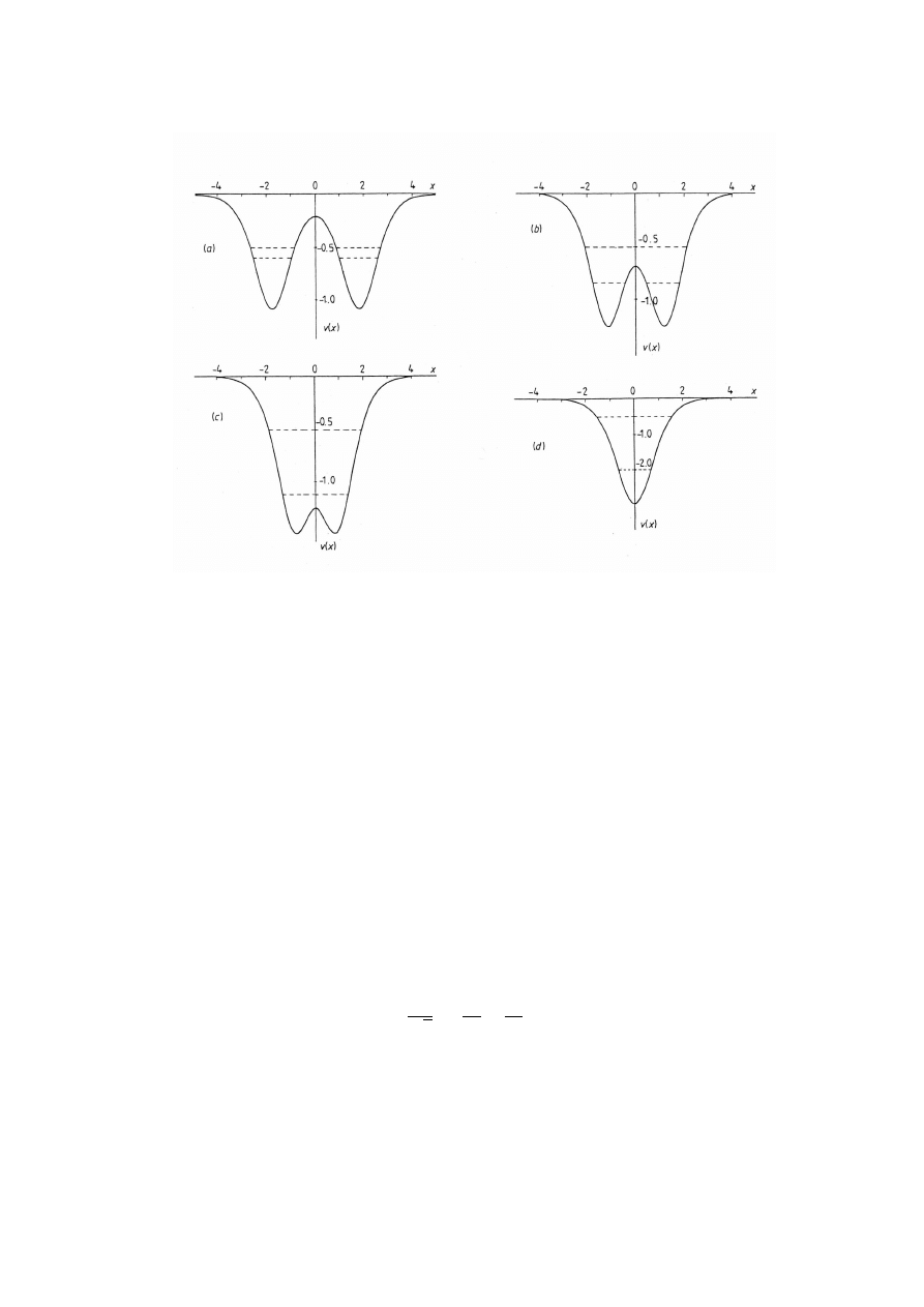
FIGURE 7.

Symmetric reflectionless potentials with bound states at energies E

= −

/2 and E

−

/2 for

= 1 and

= (a)1.1, (b) 1.3, (c) 1.5, (d) 2.0. The locations of the bound levels are indicated

by broken lines.

4.3. Potentials with an arbitrary number of bound states

By an extension of the procedure outlined in the last two sections it is possible to

construct a hierarchy of Hamiltonians with successively increasing number of bound
states starting from the Hamiltonian H

with no bound states [21, 36]. Denoting the

Hamiltonian with n bound states by H

and the ground state energy of H

by E

= −

/2 ,

n−1

> . . . >

(178)

the Hamiltonian hierarchy is given by

= A

−
m−1

+
m−1

) + E

= H

m−1

−
m−1

), A

+
m−1

)

m = 1, 2, . . . , n ,

(179)

where

±
m−1

) =

√

m−1

)

(180)

and

m−1

) is a non-normalizable nodeless solution of the eigenvalue equation for

m−1

at energy E

which lies below the ground state of H

m−1

. The potentials in the

hierarchy are related by

= V

m−1

−

m−1

) .

(181)

The ground state eigenfunction of H

is given by

) ∼

m−1

)

(182)

while all the other eigenfunctions of H

are given in terms of the eigenfunctions of H

m−1

) ∼ A

−
m−1

)

m−1

) ,

i = 1, 2, . . . , m − 1 ,

m = 1, 2, . . . , n .

(183)

This network of interrelated eigenfunctions can be disentangled to expresss all eigen-
functions of H

in terms of the solutions in the reference potential V

. Iteration of

Eq. (181) shows that the potential with n bound states is related to V

= V

−

[ln

)

) . . .

n−1

)] .

(184)

It is possible to express the product of eigenfunctions in the above equation in terms
of the solutions

) in the potential V

for various energies E

. It is then possible to

express V

in the form

= V

−

ln det D

(185)

where the matrix D

is given by

]

j−1

) ,

j, k = 1, 2, . . . , n .

(186)

The eigenfunctions for the potential V

may be expressed in the form

) ∼

−1

i = 1, 2, . . . , n .

(187)

The proof that the elements in the last column of the inverse of the matrix D

are indeed

the eigenfunctions for V

in Eq. (185) with eigenenergies E

, i = 1, 2, . . . , n, is straight-

forward but involves a long algebraic calculation. The requirement that

m−1

m = 1, 2, . . . , n, be nodeless can be met by choosing the non-normalizable solutions

), m = 1, 2, . . . , n, such that the determinant of D

has no zeros. The eigenfunc-

tion relation given in Eq. (183) can be extended to positive energies to show that the
reflection coefficient of V

is related to the reflection coefficient of V

m−1

(k) =

− ik

+ ik

m−1

(k) .

(188)

Iteration of this relation gives

(k) =

∏

m=1,2,...,n

− ik

+ ik

¶#

(k) .

(189)

Eqs. (185)-(187) provide a recipe for constructing potentials with bound states at speci-
fied energies E

and reflection coefficient for positive energies given by Eq. (189).

The algorithm for constructing reflectionless potentials with n bound states is a par-

ticular case of the procedure given above corresponding to the choice V

= 0. Since

(k) = 0 when V

= 0, R

(k) also vanishes. The free particle solutions at energies E

are given by

) =

exp

x +

+ (−)

j+1

exp

−

x −

¢i

(190)

where

are arbitrary phase factors. For odd values of j,

) is a cosh function and

hence nodeless while for even values of j,

) is a sinh function with a single node.

Such a choice of solutions ensures that det D

has no zeros. A symmetric reflectionless

potential with n bound states may be obtained by choosing

= 0 for all values of j.

The potential so obtained is given by

nSR

= −

ln det D

nSR

(191)

where the elements of the matrix D

nSR

are given by

nSR

]

(

)

j−1

exp(

x) + (−1)

j+k

exp(−

(192)

The unnormalized eigenfunctions of this potential may be given in terms of the elements
in the column n of the inverse of the matrix D

nSR

and the normalized eigenfunctions may

be written in the form

nSR

) =

∏

k6=i

−

1/2

−1
nSR

i = 1, 2, . . . , n .

(193)

The relationship of this representation of the symmetric reflectionless potentials to other
apparently different representations of the same potential can be established.

It can be shown [36] that the symmetric reflectionless potential with n bound states

may be represented in terms of the normalized bound state eigenfunctions in the form

nSR

= −2

∑

j=1

nSR

)

(194)

which is a generalized form of the results given in Eqs. (157) and (176) for the cases
n = 1 and n = 2.

The analysis of Kay and Moses [37] and the n-soliton solution of the Korteweg-

deVries equation [38, 39, 40] lead to the result that the symmetric reflectionless potential
may be expressed in terms of a matrix M with elements

(x)

(195)

where

is the Kronecker delta function and

(x) = C

exp(−

x) ,

∏

k6= j

−

(196)

in the form

V = −

ln det M .

(197)

It can be shown that the matrices M and D

nSR

are related by

M = 2GA

−1

nSR

−1

(198)

where the elements of G and A are given by

i j

∏

k6= j

−

1/2

i j

i−1

exp(

x) .

(199)

It is clear that

det A

∝

exp

∑

(200)

Using Eqs. (198)-(200) it is easy to show that

ln det M =

ln det D

nSR

(201)

leading to the result that the instantaneous n-soliton solution of the KdV equation given
by Eqs. (195)-(197) is identical to the symmetric reflectionless potential constructed
using the methods of Supersymmetric Quantum Mechanics. These ideas will be further
explored in the next subsection.

4.4. Backlund transformation, KdV equation and supersymmetry

A potential of the form given in Eq. (154) can be regarded as the instantaneous one-

soliton solution V

(x) = v

(x, 0) of the Korteweg-deVries equation [38] in the form

∂

− 12v

∂

v(x,t) = 0 ,

(202)

with v = v

. The solution for all t is

(x,t) = −

sech

x − 4

t − tanh

−1

(203)

and the soliton travels with a velocity proportional to its amplitude. The n-soliton
solution of the KdV equation (202) has been studied extensively [37, 39, 40]. The time
dependent n-soliton solution may be given in the form of Eqs. (195)-(197) with the
choice of

(x) = C

exp

−

x + 4

(204)

by endowing the basis functions with a time dependence of a specific form. It is this
specific time dependence that guarantees that the n-soliton solution satisfies the partial
differential Eq. (202). Similarly, a time dependence for the same potential constucted
using SUSY and given by Eqs. (184)-(186) and (190) can be introduced by allowing the
phases

to have a time dependence of the form

(t) =

(0) − 4

t .

(205)

Such a choice of time dependence guarantees that the potential V

satisfies the KdV

equation (202). It is possible to verify these assertions by a long calculation.

It is possible to consider other choices of time dependence for the phases. It can be

shown that if the phases are allowed to vary with time in the form

(t) =

(0) − 2

m−1

t ,

(206)

where the index m can take all odd values ≥ 3 then each of these cases can lead to a
solution of a member of the Kadomtsev-Petviashvili (KP) hierarchy studied by Caudrey
et al. [41]. m = 3 leads to the KdV equation (202) while m = 5, 7, . . . lead to higher
members of the KP hierarchy (Sukumar [42]). For this class of non-linear equations the
n-soliton solution is given by Eqs. (185), (186), (190) and (206). For example m = 5
leads to the non-linear equation

∂

− 20V

∂

− 40

∂

+ 120V

∂

V (x,t) = 0 ,

(207)

which has been studied by Sawada and Kotera [43] and Caudrey et al [41].

In the context of the KdV equation the transformations of solutions possessing n − 1

solitons to those with n solitons are known as Backlund transformations [44]. The
Backlund transformation for the KdV equation can be understood as follows. If we
consider a function F(x,t) satisfying a modified KdV equation of the form

G(x,t) ≡

∂

+ 12

− F

∂

= 0 ,

(208)

then it can be established that the function v(x,t) defined by

v(x,t) ≡

−

∂

−

(209)

can be shown to satisfy the KdV equation since Eq. (202) is equivalent to the equation

2FG −

∂

= 0 ,

(210)

which is clearly satisfied because F satisfies Eq. (208). Also it is evident that by similar
reasoning

2FG +

∂

= 0 ,

(211)

which implies that the function ˜

v(x,t) is defined by

v(x,t) ≡

∂

−

(212)

also satisfies the KdV equation (202). With suitable boundary conditions on F, one can
interpret ˜

v as an n-soliton solution if v is an (n − 1)-soliton solution. By eliminating F

the relation between v and ˜

v may be established to be

∂

h¡

v + ˜

v +

1/2

= ˜v − v .

(213)

We now show that this relation between v and ˜

v is consistent with the relation between

supersymmetric partner potentials defined by Eqs. (178)-(182). If we define the function

F(x) =

) .

(214)

then using Eqs. (178)-(182) it is easy to show that the potentials V

and V

n−1

can be

written in terms of F in the form

F −

n−1

−

F −

(215)

The above equations are identical to Eqs. (209) and (212) which define v and ˜

v. Thus Su-

persymmetric Quantum Mechanics enables the identification of the function F defined
by the Backlund transformation (Eq. (209)) for the KdV equation as the logarithmic
derivative of the ground state eigenfunction of the potential V

(x,t) which supports n

bound states where the time dependence arises from the time dependence of the

Eqs. (190) and (205). The above argument can be extended to interpret the Backlund
transformation for the entire system of non-linear equations defined by the KP hierar-
chy.

4.5. Summary

We have shown that by repeatedly using the algebra of supersymmetry in a step

by step fashion it is possible to construct potentials with bound states at arbitrary

energies. It has been shown that the non-normalizable solutions in a reference potential
which supports no bound states constitute the input in this construction. The reflection
coefficient of the potential with n bound states constructed by this procedure is related
to the reflection coefficient in the reference potential. V

is in general not only a function

of the n bound state energies E

but also a function of n parameters

, i = 1, 2, . . . , n.

characterizes a particular linear superposition of the two linearly independent non-

normalizable solutions in the reference potential V

at energy E

can take such values

that ensure that the determinant of D

is free of zeros.

By choosing the reference potential to be V

= 0 reflectionless potentials with n bound

states may be constructed. The reflectionless potential so obtained is not necessarily a
symmetric function of x. By choosing the parameters

to have specific values sym-

metric reflectionless potentials can be constructed. The resulting symmetric potential is
identical to the one constructed from the n-soliton solution of the KdV equation. Sym-
metric reflectionless potentials are unique and interesting because they are specified en-
tirely by their bound states. They have been shown to provide good approximations to
confining potentials, such as those which confine quarks, in the range of energies actu-
ally probed by the levels (Thacker et al. [45], Quigg and Rosner [46], Kwong and Rosner
[47]). Kwong and Rosner have constructed an approximation to a quarkonium potential
on the basis of information about its nS levels. Using the energies and leptonic widths
of 10 levels below the flavour threshold Kwong and Rosner have used the algorithm for
constructing symmetric reflectionless potentials to construct a potential V (r). Calcula-
tions such as these provide information on the distance scale over which t ¯t bound state
information is likely to shed light on the interquark force.

We have shown that it is possible to identify a hierarchy of non-linear equations of

the KdV type which have the property that the n-soliton solution of these equations can
be explicitly given in analytic form. The connection between SUSYQM and Backlund
transformations provides interesting insights and enables a physical interpretation of the
function that is used to construct the Backlund transformation. The symmetries which
lead to an infinite number of conservation laws in integrable systems such as the KdV
equation have already been recognized as being related to Kac-Moody algebras. It is
clear that we can now add supersymmetry to the list of properties connected with such
systems.

We have also shown that the symmetric reflectionless potentials may be expressed in

terms of the normalized bound state eigenfunctions in a particularly simple form. It is
clear that the construction based on supersymmetry not only agrees with calculations
based on other procedures but also provides unique insight into the structure of symmet-
ric reflectionless potentials and the structure of the multi-soliton solutions of the KdV
hierarchy and the Backlund transformations associated with these non-linear equations.

5. PAIRS OF SUSY TRANSFORMATIONS FOR THE RADIAL

SCHRÖDINGER EQUATION

It was shown in an earlier lecture that it is possible to identify four different transforma-
tions by which one can find a supersymmetric partner to a given radial Schrödinger equa-

tion. The modifications of the Jost function and the singularity structure in the asymp-
totic region r →

∞

and in the region r → 0 for the 4 types of SUSY transformations

were identified. Each of the transformations alters the spectral density in a specific man-
ner and either removes or adds a bound state or maintains the same spectrum. In this
lecture we study how pairs of SUSY transformations may be used to modify or maintain
the spectrum with or without altering the spectral density. An exactly solvable example
is used to illustrate the procedure.

5.1. Classification of the four types of SUSY transformations

In §2 four different transformations of the radial Schrödinger equation were identified

by T

, T

and T

. The potentials, eigenstates and phase shifts and the Jost function

after the supersymmetric transformation were denoted by adding a tilde. The different
types of transformations were distinguished by adding a suffix. In this lecture we adopt
the same notations for single transformations. Succesive transformations will be indi-
cated by adding further suffixes and tildes. We also use the same notation as in §2 that
the regular solution at a given energy ˜

E = − ˜

/2 will be denoted by

(r) and the Jost

solution by

(r). It was shown that these functions obey the boundary conditions

lim

r→0

(r) =

(l+1)

(2l + 1)!!

lim

r→

∞

(r) ∼ exp( ˜

r) ,

(216)

lim

r→0

(r) ∼ r

−l

lim

r→

∞

(r) ∼ exp(− ˜

r) .

(217)

We also use the notation

(m)

(r) is an abbreviation for

(r, E

(m)

It was shown in §2 that for all the four types of transformations the potential is

unaltered in the region r →

∞

and that each of the transformations produces an alteration

of the potential in the region of small and medium r and near r → 0 the alteration of
the potential is equivalent to altering the angular momentum l in the centrifugal part
l(l + 1)/r

of the potential V (r) corresponding to a definite partial wave. The changes

for the four transformations corresponding to the factorization energy E = −

/2 were

identified as:

F = F

k − i

, lim

r→0

l → l + 1 ,

− tan

−1

(

/k) −

F = F

k − i

, lim

r→0

l → l − 1 ,

+ tan

−1

(

/k) +

F = F

k + i

, lim

r→0

l → l + 1 ,

+ tan

−1

(

/k) −

F = F

k + i

, lim

r→0

l → l − 1 ,

− tan

−1

(

/k) +

(218)

eliminates the ground state at E leaving the rest of the spectrum of eigenvalues

unaltered. T

adds a new ground state at E while leaving the rest of the spectrum

unaltered. T

and T

maintain the same spectrum and alter the Jost function and the

singularity of the potential at the origin. These four transformations may be viewed
as the building blocks which can be used in suitable combinations to produce desired
modifications of the spectrum, the Jost function and the singularity at the origin. We
next study pairs of SUSY transformations and the alteration of the spectrum and the Jost
function that they produce.

5.2. Pairs of SUSY transformations

We consider two successive transformations performed at the same energy E. Of the

sixteen possibilities that arise from a combination of any one of the T

with any other

, it is clear when j and k are different the combination T

is equivalent to T

. Of

the remaining ten possibilities T

does not exist because it is not possible to remove

the same bound state twice and T

does not exist because the same bound state can

not be added twice. Therefore there are eight distinct possibilities for pairs of SUSY
transformations which must be considered. We now classify them.

(1) T

followed by T

removes a bound state at energy E and adds the same bound

state at the same energy. At the end of the two transformations we get a potential which
has the same spectrum as the original potential but the normalization constant of the
ground state may be altered and the Jost function is unaltered.

˜˜

= F .

(219)

The phase shifts and the normalization constants of all the excited state eigenfunctions
are unaltered. Therefore T

produces the phase-equivalent family corresponding to a

given potential.

(2) T

followed by T

removes a bound state at energy E and alters the spectral

density and the normalization constants of the remaining eigenstates. The Jost function
is modified to

˜˜

= F

(220)

The phase shifts for positive energies are unaltered. However, the resulting potential is
singular with a singularity of the form r

−2

(3) T

followed by T

removes a bound state at energy E and keeps the spectral density

unaltered which implies that the normalization constants of all the other bound states are
unaltered. The Jost function is modified to

˜˜

= F

k + i

k − i

(221)

The phase shifts for positive energies will be altered.

(4) T

followed by T

adds a bound state below the ground state of the original

potential without altering the spectral density. The normalization constants of all the
other states are left unaltered. The Jost function is modified to

˜˜

= F

k − i

k + i

(222)

The phase shifts for positive energies will, however, be altered.

(5) T

followed by T

adds a bound state below the ground state of the original

potential and alters the spectral density and the normalization constants of the other
eigenstates. The Jost function is modified to

˜˜

= F

(223)

The phase shifts for positive energies will not be altered. Hence T

produces a family

of phase-equivalent potential with a new ground state and different members of the
family will have different values for the normalization constants of the ground state.
The resulting potential is singular at the origin.

(6) T

followed by another T

maintains the same spectrum and alters the spectral den-

sity. The normalization constants of all the states are altered and the resulting potential
has r

−2

singularity at the origin. The Jost function is modified to

˜˜

= F

k + i

(224)

The phase shifts for positive energies and the normalization constants of the eigenfunc-
tions will be altered.

(7) T

followed by T

transforms the original Hamiltonian back to itself without

altering the spectral density, spectrum and the phase shifts for positive energies. In fact

˜˜

= F .

(225)

(8) T

followed by another T

is similar to case (6) and also maintains the same

spectrum, alters the spectral density and the normalization constants of all the states.
The resulting potential is a singular potential. The Jost function is modified to

˜˜

= F

k + i

(226)

The phase shifts for positive energies and the normalization constants of the eigenfunc-
tions will be altered.

The eight cases listed above exhaust the possible combinations of two SUSY trans-

formations. We now examine these cases in detail.

(1) We now show that T

followed by T

generates the phase-equivalent family to a

given potential

V (r) =

l(l + 1)

+ v(r) ,

(227)

with ground state

(0)

(r) at energy E

(0)

. After the first transformation T

which elimi-

nates the ground state of V the potential is

(r) = V (r) −

(0)

(r) .

(228)

Using the second transformation T

the eliminated state can be introduced as the new

ground state below the ground state of ˜

. It was shown in §2 that the solution in ˜

the correspoding energy may be given in the form

(r, E

(0)

) = ˜

(r, E

(0)

) cos

+ ˜

(r, E

(0)

) sin

(229)

where ˜

is the regular solution in ˜

at energy E

(0)

and ˜

is the Jost solution in ˜

the same energy and are given by

∼

(0)

(r)

(0)

(x)

dx ,

∼

(0)

(r)

∞

(0)

(x)

dx .

(230)

can be written in terms of the parameter

defined by

tan

+ 1

(231)

in the form

(r, E

(0)

) =

1 +

(0)

(x)

(0)

(r)

−1 <

∞

(232)

The potential at the end of the two transformations is given by

˜˜

1,2

(r) = V (r) −

1 +

(0)

(x)

(233)

which has a spectrum identical with that of V (r) and has normalized ground state
obtained from the inverse of ˜

in Eq. (232) in the form

˜˜

(0)
1,2

(1 +

)

1/2

(0)

(r)

1 +

(0)

(x)

(234)

The excited states at the end of the two transformations are given by

˜˜

(m)
1,2

= −

(m)

− E

(0)

−1

−
2

−
1

(m)

m = 1, 2, . . . ,

(235)

where

−
2

(0)

) =

√

−

ln ˜

−
1

√

−

(0)

(r)

(236)

The excited state eigenfunctions can be simplified to the form

˜˜

(m)
1,2

(m)

−

(m)

(r)

(m)

− E

(0)

¢ ,

(m)

(r) =

(0)

(r)

1 +

(0)

(x)

(m)

(0)

−

(0)

(m)

(237)

The Wronskian relation arising from the the Schrödinger equation considered at two
different energies in the form

(m)

(0)

−

(0)

(m)

= 2

(m)

− E

(0)

(x)

(m)

(x)dx ,

(238)

may then be used to express the excited state eigenfunctions in the form

˜˜

(m)
1,2

(r) =

(m)

(r) −

λψ

(0)

(r)

(0)

(x)

(m)

(x)dx

1 +

(0)

(x)

m = 1, 2, . . . .

(239)

From Eqs. (234) and (239) it can be established that

˜˜

1,2

(l, k) =

(l, k) ,

lim

r→0

˜˜

(m)
1,2

(r,

) = lim

r→0

(m)

(r) ,

m = 1, 2, . . . ,

lim

r→0

˜˜

(0)
1,2

(r,

) = (1 +

)

1/2

lim

r→0

(0)

(r) .

(240)

It is also clear from Eq. (218) that at the end of the two transformations T

and T

the

singularity at the origin arising from the centrifugal part of the potential is unaltered
and also that the phase shifts are unaltered. These results show that the family of po-
tentials ˜˜

1,2

(r,

) in Eq. (233) for

∞

> −1 have identical spectra, identical phase

shifts and identical normalization constants for the excited states but have different nor-
malization constants for the ground state for different values of

. Hence this family

of potentials belongs to a phase-equivalent family. These expressions for the new po-
tential and the new eigenfunctions are in agreement with the results obtained using the
Gelfand-Levitan procedure for changing the normalization constant of the ground state
[26, 30]. Thus we have shown that the Gelfand-Levitan [24] procedure for changing the
normalization constant of the ground state without changing the spectrum is equivalent
to a transformation of the type T

followed by another suitable transformation of the type

[28].

(2) We now consider T

followed by T

. The first step is the same as case (1) and leads

to the potential given by Eq. (228). The second step corresponds to a T

transformation

with the choice of value

= 0 in Eq. (229) which also corresponds to the choice

∞

in Eq. (232). Such a choice for ˜

leads to the new potential after the two transformations

of the form

˜˜

1,3

(r) = V (r) −

(0)

(x)

(241)

which has a spectrum identical with that of V (r) except for missing the ground state of

V . The eigenfunctions of ˜˜

1,3

are related to the excited state eigenfunctions of V by

˜˜

(m)
1,3

= −

(m)

− E

(0)

−1

−
3

−
1

(m)

m = 1, 2, . . . ,

(242)

where

−
3

√

−

(0)

(r)

(0)

(x)

¶¸

(243)

and A

−
1

has the same form as in Eq. (236). From these equations it can be established

using the same steps as in case (1) that

˜˜

(m)
1,3

(m)

(r) −

(0)

(r)

(0)

(x)

(m)

(x)dx

(0)

(x)

m = 1, 2, . . . ,

(244)

and that the normalization constants of the eigenfunctions are altered. It can be shown
from Eq. (241) or from Eq. (218) that

lim

r→0

˜˜

1,3

(r) =

(l + 2)(l + 3)

lim

r→

∞

˜˜

1,3

(r) =

l(l + 1)

(245)

which shows that the new potential is singular at the origin and has a short range
repulsive singularity. Eq. (218) can also be used to show that the phase shifts are
decreased by a constant amount

for all positive energies which is equivalent to saying

that the phase shifts are unaltered within modulo

. Thus a transformation of the type T

followed by a transformation of the type T

can be used to produce a singular potential

which has the same phase shifts as the original potential but has one less bound state
[48].

(3) We next consider T

followed by T

. The first step is the same as in cases (1) and

(2) and leads to the potential given in Eq. (228). The second step corresponds to a T

tranformation with the choice of value

/2 in Eq. (229) which also corresponds to

the choice

= −1 in Eq. (232). Such a choice of ˜

leads to a new potential after the

two transformations of the form

˜˜

1,4

(r) = V (r) −

∞

(0)

(x)

(246)

which has the same spectrum as V except for missing the ground state of V . The
eigenstates of the new potential can be obtained by the same procedure as for the earlier
cases and can be readily obtained by taking

= −1 in Eq. (239) to give

˜˜

(m)
1,4

(r) =

(m)

(r) −

(0)

(r)

∞

(0)

(x)

(m)

(x)dx

∞

(0)

(x)

m = 1, 2, . . . .

(247)

It can be established from this equation that the bound state normalizations are unaf-
fected. It can be shown using Eq. (218) that the phase shift relation for positive energies

˜˜

1,4

(l, k) =

(l, k) − 2 tan

−1

(0)

(248)

It can also be shown using Eq. (218) that the singularity of the potential ˜˜

1,4

at the origin

is unaltered. The expressions for the new potential and the new eigenfunctions [28] are
identical to the results given by Abraham and Moses [26]. Thus the Gelfand-Levitan
procedure to eliminate the ground state without introducing additional singularities
at the origin is equivalent to a transformation T

which eliminates the ground state

followed by a transformation T

which removes the additional singularity at the origin

which is introduced by the first transformation. The resultant potential after the two
transfromations is non-singular.

(4) We next consider T

followed by T

. The transformation T

may be used at energy

E below the ground state of V to produce a new potential which has the same spectrum
as that of V as described in §2.6. The T

transformation is implemented by considering

the regular solution

(r, ˜

E) for the potential V (r). After the T

transformation the new

potential is

(r, ˜

E) = V (r) −

(r, ˜

E) .

(249)

We now apply a T

transformation at the energy ˜

E to introduce a new bound state below

the ground state of V . One of the solutions at energy ˜

E in the potential ˜

is given by

(r, ˜

(250)

and the second linearly independent solution is, therefore, given by

(r, ˜

E) =

(r, ˜

(x, ˜

dx .

(251)

By studying the limiting behaviour of

and

it can be established that the regular

and the Jost solution in ˜

are indeed proportional to

and

respectively. Hence using

the general solution

(r, ˜

) =

(r, ˜

E) sin

(r, ˜

E) cos

(252)

the new potential after the two transformations may be given in the form

˜˜

3,2

(r, ˜

) = V (r) −

cos

+ sin

(x, ˜

(253)

which has a ground state eigenvalue at ˜

E while all the other eigenvalues are identical to

those of V . The normalized ground state of ˜˜

3,2

is given by

˜˜

(0)
3,2

(r, ˜

) =

(sin

cos

)

1/2

(r, ˜

cos

+ sin

(x, ˜

(254)

Eq. (254) shows that the parameter

determines the normalization constant of the

ground state.

/4 corresponds to choosing the normalization constant as 1 and

for this choice the resulting potential is

˜˜

3,2

(r, ˜

/4) = V (r) −

1 +

(x, ˜

(255)

which has the ground state eigenfunction

˜˜

(0)
3,2

(r, ˜

E) =

(r, ˜

1 +

(x, ˜

(256)

The excited state eigenfunctions are given by

˜˜

(m)
3,2

(r) = −

(m)

− E

(0)

−1

−
2

−
3

(m)

(r) ,

m = 1, 2, . . . ,

(257)

where

−
2

√

−

1 +

(x, ˜

(r, ˜

−
3

√

−

(r, ˜

(258)

Using the same method as in previous cases the expression for the excited state eigen-
functions can be brought to the form

˜˜

(m)
3,2

(r, ˜

E) =

(m)

(r) −

(r, ˜

(x, ˜

(m)

(x)dx

1 +

(x, ˜

m = 1, 2, . . . .

(259)

It is easy to show that

lim

r→0

˜˜

(m)
3,2

(r) = lim

r→0

(m)

(r) .

(260)

Thus the normalization constants of the eigenfunctions are left unaltered. Eq. (218) can
be used to show that the singularity of the potential at the origin is unaltered after the two
transformations. It can also be shown that the phase shift relation for positive energies is

˜˜

3,2

(l, k) =

(l, k) + 2 tan

−1

(261)

The expressions for the new potential and the new eigenfunctions [28] derived above are
in agreement with the results derived using the Gelfand-Levitan method [26].

The family of potentials ˜˜

3,2

(r, ˜

) in Eq. (253) lead to identical phase shifts and

the normalization constants for the excited states of the potentials ˜˜

3,2

(r, ˜

) for

various values of

in the range 0 <

/2, are the same. The parameter

affects

the normalization constant of the ground state. The family of potentials ˜˜

3,2

(r, ˜

)

have identical spectra, identical phase shifts and identical normalization constants for
all states except the ground state and is, therefore, a phase-equivalent family. Thus a
tranformation of the type T

followed by a transformation of the type T

enables the

generation of a family of potentials which have a new ground state but without altering
the spectral density and without altering the singularity of the potential at the origin.

(5) We next consider T

followed by T

. This sequence is very similar to case (4)

except that in the first step involving the transformation T

the Jost solution

(r, ˜

E) is

used instead of the regular solution

(r, ˜

E) in the potential V . After the T

transformation

the new potential is

(r, ˜

E) = V (r) −

(r, ˜

E) .

(262)

We now apply a T

transformation at the energy ˜

E to introduce a new bound state below

the ground state of V . By identifying the general solution in ˜

at energy ˜

E in the form

(r, ˜

) =

cos

+ sin

∞

(x, ˜

(r, ˜

(263)

the new potential after the two transformations may be given in the form

˜˜

4,2

(r, ˜

) = V (r) −

cos

+ sin

∞

(x, ˜

(264)

which has a ground state eigenvalue at ˜

E while all the other eigenvalues are identical to

those of V . The normalized ground state of ˜˜

4,2

is given by

˜˜

(0)
4,2

(r, ˜

) =

(sin

cos

)

1/2

(r, ˜

cos

+ sin

∞

(x, ˜

(265)

Eq. (265) shows that the parameter

determines the normalization constant of the

ground state. For

/4 the resultant potential after the two transformations is

˜˜

4,2

(r, ˜

E) = V (r) −

1 +

∞

(x, ˜

(266)

which has the ground state eigenfunction

˜˜

(0)
4,2

(r, ˜

E) =

(r, ˜

1 +

∞

(x, ˜

(267)

The excited state eigenfunctions are given by

˜˜

(m)
4,2

(r) = −

(m)

− E

(0)

−1

−
2

−
4

(m)

(r) ,

m = 1, 2, . . . ,

(268)

where

−
2

√

−

1 +

∞

(x, ˜

(r, ˜

−
4

√

−

(r, ˜

(269)

Using the same methods as in the previous cases the excited state eigenfunctions can be
shown to be given by

˜˜

(m)
4,2

(r, ˜

E) =

(m)

(r) −

(r, ˜

∞

(x, ˜

(m)

(x)dx

1 +

∞

(x, ˜

m = 1, 2, . . . .

(270)

It can be shown that the normalization constants of the eigenfunctions are left unaltered.
It can also be shown using Eq. (218) that the phase shifts are increased by a constant
amount

for all positive energies which is equivalent to saying that the phase shifts are

unaltered within modulo

. However

lim

r→0

˜˜

4,2

(r) =

(l − 2)(l − 1)

lim

r→

∞

˜˜

4,2

(r) =

l(l + 1)

(271)

which shows that ˜˜

4,2

has a component which has a short range attractive r

−2

singularity

in addition to the usual centrifugal potential.

Thus we have shown that the application of a transformation of the type T

followed

by a transformation of the type T

enables the construction of singular potentials which

have the same phase shifts as the original potential but which have an additional bound
state at a chosen energy. The family of potentials ˜˜

4,2

(r, ˜

), for various values of

the range 0 <

/2, have identical phase shifts and identical normalization constants

for the excited states but have different normalization constants for the ground state and
belong to a family of phase-equivalent potentials.

(6) We now consider two successive T

transformations performed at the same energy

E below the ground state of V . After the first T

transformation using the regular solution

in the potential V the new potential ˜

has the form given by Eq. (249). The second T

transformation is performed using the choice

/2 in Eq. (252) so that ˜

(r) =

(r)

which is defined by Eq. (251). The resulting potential after the two transformations is
then given by

˜˜

3,3

(r, ˜

E) = V (r) −

(x, ˜

(272)

which leads to a spectrum of eigenvalues which is identical with that for V . The trans-
formed eigenstates may be shown to be given by

˜˜

(m)
3,3

(r) =

(m)

(r) −

(r, ˜

(x, ˜

(m)

(x)dx

(x, ˜

m = 0, 1, . . . .

(273)

It can be established that the normalization constants of the eigenfunctions and the
spectral density are altered. Using Eq. (218) the phase shifts for positive energies can
be shown to be related by

˜˜

3,3

(l, k) =

(l, k) + 2 tan

−1

−

(274)

It can also be shown that

lim

r→0

˜˜

3,3

(r, ˜

E) =

(l + 2)(l + 3)

lim

r→

∞

˜˜

3,3

(r, ˜

E) =

l(l + 1)

(275)

which shows that ˜˜

V is a singular potential. Thus two successive T

transformations may

be used to produce a new singular potential which has the same spectrum as V but has
different phase shifts and different normalization constants.

(7) We next consider T

followed by T

. The first step is the same as in case (6). In the

second step the T

transformation is performed using the choice

= 0 in Eq. (252) so

that ˜

(r) =

(r) defined by Eq. (250). With this choice it is clear that the potential after

the two transformations is identical to the original potential V (r) since

(r)

(r) = 1.

Thus T

restores the original Hamiltonian and all the eigenstates and phase shifts are

unaltered. Thus T

followed by T

performed at the same energy is equivalent to the

identity transformation.

(8) The last combination we consider is two successive T

transformations at the same

energy ˜

E below the ground state of V . After the first T

transformation using the Jost

solution

in the potential V the new potential ˜

has the form given by Eq. (262). The

second T

transformation is performed by using the choice

/2 in Eq. (263) so that

the new potential after the two transformations is given by

˜˜

4,4

(r, ˜

E) = V (r) −

∞

(x, ˜

(276)

which has the same spectrum as that for V (r). The transformed eigenfunctions may be
shown to be given by

˜˜

(m)
4,4

(r) =

(m)

(r) −

(r, ˜

∞

(x, ˜

(m)

(x)

∞

(x, ˜

m = 0, 1, . . . .

(277)

It can be established that the spectral density is altered and that the normalization
constants of the eigenfunctions are altered. Using Eq. (218) it can be seen that the phase
shifts for positive energies are related by

˜˜

4,4

(l, k) =

(l, k) − 2 tan

−1

(278)

It can also be shown that

lim

r→0

˜˜

4,4

(r, ˜

E) =

(l − 2)(l − 1)

lim

r→

∞

˜˜

4,4

(r, ˜

E) =

l(l + 1)

(279)

which shows that ˜˜

4,4

is a singular potential. Thus two successive T

transformations

may be used to produce a new singular potential which has the same spectrum as V but
has different phase shifts and different normalization constants.

The new eigenfunctions after two transformations given by Eqs. (239), (244), (247),

(259), (270), (273) and (277) can all be expressed as the ratio of 2 determinants. The new
potential can be expressed as a determinant of a matrix M. These identifications enable
the extension of the procedure outlined in this lecture to the elimination or addition of an
arbitrary number of states or the generation of isospectral Hamiltonians after a number
of transformations at different energies. We now indicate the structure of the theory for
the seven nontrivial cases considered earlier.

For case (1) the matrix M has just a single element when a pair of transformations are

used at a single energy and is given by

= 1 +

(0)

(x)

dx .

(280)

In terms of a second matrix ˜˜

M given by

˜˜

M =

(0)

(x)

(m)

(x)dx

(0)

(r)

(m)

(r)

(281)

the eigenfunction relation given in Eq. (239) may be expressed in the form

˜˜

(m)
1,2

det ˜˜

det M

(282)

For case (2) the matrix M has element

(0)

(x)

dx ,

(283)

and ˜˜

M is given by

˜˜

M =

(0)

(x)

(m)

(x)dx

(0)

(r)

(m)

(r)

(284)

The eigenfunction relation in Eq. (244) can be written in terms of these matrices as

˜˜

(m)
1,3

det ˜˜

det M

(285)

For case (3) the matrix M has element

∞

(0)

(x)

dx ,

(286)

and ˜˜

M is given by

˜˜

M =

∞

(0)

(x)

(m)

(x)dx

(0)

(r)

(m)

(r)

(287)

The eigenfunction relation in Eq. (247) may then be written in the form

˜˜

(m)
1,4

det ˜˜

det M

(288)

For case (4) M is given by

= 1 +

(x, ˜

dx ,

(289)

and the matrix ˜˜

M has the form

˜˜

M =

(x, ˜

(m)

(x)dx

(r, ˜

(m)

(r)

(290)

The eigenfunction relation in Eq. (259) may be given in the form

˜˜

(m)
3,2

det ˜˜

det M

(291)

For case (5)

= 1 +

∞

(x, ˜

dx ,

(292)

and

˜˜

M =

∞

(x, ˜

(m)

(x)dx

(r, ˜

(m)

(r)

(293)

The eigenfunction relation in Eq. (270) may be given in the form

˜˜

(m)
4,2

det ˜˜

det M

(294)

For case (6)

(x, ˜

dx ,

(295)

and

˜˜

M =

(x, ˜

(m)

(x)dx

(r, ˜

(m)

(r)

(296)

The eigenfunction relation in Eq. (273) may be written in the form

˜˜

(m)
3,3

det ˜˜

det M

(297)

Similarly for case (8)

∞

(x, ˜

dx ,

(298)

and

˜˜

M =

∞

(x, ˜

(m)

(x)dx

(r, ˜

(m)

(r)

(299)

The eigenfunction relation in Eq. (277) may be given in the form

˜˜

(m)
4,4

det ˜˜

det M

(300)

5.3. Examples

The theory outlined in the last section may be illustrated with some exactly solvable

examples. To illustrate the first three cases we consider the potential

V (r) = −3sech

r ,

(301)

which supports a single bound state at E = −1/2 with eigenfunction

(0)

(r) =

√

1 − Z

Z = tanh r .

(302)

It is easy to show that

∞

(0)

(x)

dx = 1 − tanh

r ,

(303)

(

(0)(x))

dx = tanh

r .

(304)

By using the procedure for case (1) the family of phase-equivalent potentials in Eq. (233)
can be given as

˜˜

1,2

= −3

sech

1 +

tanh

1 + 2

tanh rsech

r −

tanh

(305)

For values of

∞

< −1, the family of potentials ˜˜

1,2

have a single bound state at the

same energy but differ in the normalization constant of the ground state eigenfunction.

= 0 corresponds to the original potential V .

The method used for case (2) leads to the potential in Eq. (241) which in this example

becomes

˜˜

1,3

(r) =

sinh

(306)

which is repulsive singular potential which supports no bound states and is phase-
equivalent to V (r).

The method used for case (3) leads to the potential in Eq. (246) which in this example

becomes

˜˜

1,4

(r) = −3

sech

1 + tanh r + tanh

(307)

which is an attractive non-singular potential which supports no bound states but has the
phase shifts altered as specifed by Eq. (248).

We next examine V = 0 and the transformation energy ˜

E = − ˜

/2. The regular

solution is

= sinh ˜

r ,

lim

r→0

= ˜

r ,

lim

r→

∞

∼ exp(+ ˜

r) ,

(308)

and the Jost solution is

= exp(− ˜

r) ,

lim

r→0

= 1 ,

lim

r→

∞

= exp(− ˜

r) .

(309)

The potential arising from a T

transformation is

sinh

(310)

which is a repulsive potential. The integral relation

sinh

rdx ≡ F =

sinh 2 ˜

r − 2 ˜

4 ˜

(311)

may be used to find the potential in Eq. (253) in the form

˜˜

3,2

sinh

(cot

+ F)

−

sinh 2 ˜

cot

+ F

(312)

which is a non-singular family of phase-equivalent potentials for 0 <

/2 with

normalized ground state eigenfunctions given by

˜˜

3,2

√

sin

cos

sinh ˜

cos

+ F sin

(313)

The potential after the T

transformation is ˜

= 0. Using the integral relation

∞

(

(x))

dx =

exp(−2 ˜

2 ˜

(314)

the potential in Eq. (264) in this example becomes

˜˜

4,2

= − ˜

sech

( ˜

r +

) ,

= ln (2 ˜

cot

) ,

(315)

which is also a family of phase-equivalent potentials for 0 <

/2, with ground state

eigenfunctions given by

˜˜

4,2

∼

exp(− ˜

cos

+ sin

exp(−2 ˜

(316)

The potential after two T

transformations given by Eq. (272) in this example is

˜˜

3,3

sinh

−

sinh 2 ˜

r ,

(317)

where F is given by Eq. (311).

The potential after two T

transformation given by Eq. (276) in this example gives

˜˜

4,4

= 0. This completes the list of transformed potentials after two T transformations.

5.4. Summary

We have studied the properties of potentials and eigenfunctions arising from two

successive supersymmetric transformations performed at the same energy. We have
illustrated the procedure using an exactly solvable example. The method developed in
this lecture may be extended to eliminate or add an arbitrary number of states or alter the
phase shifts without altering the spectrum. The generalized procedure for accomplishing
the above mentioned tasks will be the subject of the next lecture.

6. SEQUENCE OF SUSY TRANSFORMATIONS, REGULAR AND

SINGULAR POTENTIALS AND APPLICATIONS

The procedure discussed in the previous lectures for the modification of the spectrum
of a potential corresponding to a radial Schrödinger equation by a two-step procedure
may be generalized to discuss the removal or addition of an arbitrary number of bound
states to a given spectrum or to generate the phase equivalent families corresponding
to given potentials. The singular potentials arising from the two-step procedure have
proved useful in understanding the relation between deep and shallow potentials both of
which have been used with some success in describing a variety of scattering problems
in Nuclear Physics. Some examples will be discussed.

6.1. Elimination of m bound states and non-singular potentials

In §5 it was shown that a tranformation of the type T

followed by a transformation

of the type T

may be used to remove the ground state of a potential V (r) for a

definite partial wave without altering the spectral density and the normalization constants
of all the excited state eigenfunctions of V (r). The phase shifts for positive energies
will, however, be altered in a definite manner. The resulting potential and the new
eigenfunctions were given in terms of the matrices M and ˜˜

M defined by

∞

(0)

(x)

dx ,

(318)

and

˜˜

(n)

∞

(0)

(x)

∞

(0)

(x)

(n)

(x)dx

(0)

(r)

(n)

(r)

n = 1, 2, . . . ,

(319)

in the form

˜˜

1,4

(r) = V (r) −

ln (det M)

(320)

˜˜

(n)
1,4

(r) =

det ˜˜

(n)

det M

n = 1, 2, . . . .

(321)

The phase shifts for positive energies were related by

˜˜

1,4

(l, k) =

(l, k) − 2 tan

−1

(0)

(322)

It was also shown that the two transformations T

taken together do not introduce any

additional singularities in the new potential.

The procedure used for eliminating a single bound state may be generalized to the

case of elimination of an arbitrary number m of bound states as follows. Let V

be a

potential with bound states given by

(1)

(2)

. . . E

(n)

(1)

(2)

. . .

(n)

(323)

determined from the solutions to the radial Schrödinger equation

−

l(l + 1)

(r) − E

( j)

(r) = 0 ,

j = 1, 2, . . . , n .

(324)

The eigenfunction set in Eq. (323) may be taken to be an orthonormal set. The incom-
plete overlap integrals may be defined by

∞

( j)

(x)

(k)

(x)dx ,

j, k = 1, 2, . . . , n ,

(325)

( j)

(x)

(k)

(x)dx ,

j, k = 1, 2, . . . , n .

(326)

The two matrices F and G are related by F + G = I where I is the unit matrix of dimen-
sion [n, n]. By using the orthonormal property of the eigenfunctions and the Wronskian
relation between two solutions of the Schrödinger equation in the same potential at two
different energies, F

and G

can also be written as

= −G

(k)

− E

( j)

(r)

(k)

(r) −

(k)

(r)

( j)

(r)

j 6= k .

(327)

Let V

be the potential generated from V

by the application of a sequence consisting

of m pairs of T

and T

transformations for eliminating the lowest m bound states of V

so that the bound states of V

are given by

(m+1)

(m+2)

. . . E

(n)

(m+1)

(m+2)

. . .

(n)

(328)

Then it may be shown by a generalization of the method for eliminating a single bound
state that in terms of a matrix M with elements given by

= F

j, k = 1, 2, . . . , m ,

(329)

the potential V

with n − m bound states may be given as

= V

−

ln (det M) .

(330)

The eigenfunctions of V

are related to those of V

(i)

det ˜˜

(i)

det M

i = m + 1, m + 2, . . . , n ,

(331)

where the elements of ˜˜

(i)

are

˜˜

(i)

= M

j, k = 1, 2, . . . , m ,

˜˜

(i)

j,m+1

∞

( j)

(x)

(i)

(x)dx = F

j = 1, 2, . . . , m ,

˜˜

(i)
m+1,k

(k)

(r) ,

k = 1, 2, . . . , m ,

˜˜

(i)
m+1,m+1

(i)

(r) ,

i = m + 1, m + 2, . . . , n .

(332)

Eqs. (329)-(332) provide a recipe for constructing a new potential by removing m
bound states and which does not have any additional singularities present which are not
already present in V

. This recipe is the same as the recipe based on the Gelfand-Levitan

equations. The phase shifts in the new potential V

for positive energies are related to

the phase shifts in V

˜˜

(l, k) =

(l, k) − 2

∑

j=1

tan

−1

( j)

(333)

where

( j)

−2E

( j)

. In the limit k → 0 the phase shift decreases by m

in agreement

with the general result for a potential with m fewer bound states. In the limit k →

∞

the

phase shifts in the two potentials are identical.

The expression for the new eigenfunctions in Eq. (331) may also be given in other

forms by expanding the determinant in the numerator and using the definition of the
elements of the inverse of a matrix as the ratio of two determinants. This leads to the
expression

(i)

−

∑

k=1

∑

j=1

(k)

−1

k j

i = m + 1, m + 2, . . . , n .

(334)

Since the index j in the above equation can only take values in the range 1 ≤ j ≤ m and
the index i takes values m < i ≤ n the matrix element F

may be replaced by −G

that Eq. (334) may also be given in the form

(i)

∑

k=1

∑

j=1

(k)

−1

k j

i = m + 1, m + 2, . . . , n .

(335)

It may be shown that in this form the above equation may be extended to allow the index
i to take all values in the range [1, n] to define a set of solutions in V

at the energies at

which the bound states have been removed. It can be shown that these non-normalizable
solutions in V

at the energies corresponding to the removed bound states satisfy

( j)

∑

k=1

(k)

−1

k j

(336)

In terms of the solutions to the linear equations

∑

j=1

k j

( j)

k = 1, 2, . . . , m .

(337)

the normalizable bound state eigenfunctions of V

may be given as

(i)

−

∑

k=1

(k)

i = m + 1, m + 2, . . . , n .

(338)

Thus by constructing the matrix M and solving the linear equations (337) to find

(k)

once it is possible to find all the eigen functions of V

using Eq. (338). It may be

shown that the expression for the new potential in Eq. (330) can be further simplified by
expanding the logarithmic derivative to get

ln (det M) =

∑

k=1

(k)

(r)

(k)

(r) ,

(339)

so that the modified potential may be expressed in the form

(r) = V

(r) −

∑

k=1

(k)

(r)

(k)

(r)

(340)

In this form the potential arising from the removal of m bound states is expressed as a
symmetric function of the solutions in the old and new potentials at the energies at which
the bound states have been removed.

6.2. Elimination of m bound states and singular potentials

In §5 it was shown that a transformation of the type T

followed by a transformation

of the type T

may be used to remove the ground state of a potential V (r) without

altering the phase shifts for positive energies. However, the normalization constants of
the eigenstates and the spectral density are altered at the end of the two transformations.
The resulting potential and the new eigenfunctions were given in terms of the matrices
N and ˜˜

N defined by

(0)

(x)

dx ,

(341)

and

˜˜

(n)

(0)

(x)

(0)

(x)

(n)

(x)dx

(0)

(r)

(n)

(r)

n = 1, 2, . . . ,

(342)

in the form

˜˜

1,3

(r) = V (r) −

ln (det N) ,

(343)

˜˜

(n)
1,3

(r) =

det ˜˜

(n)

det N

n = 1, 2, . . . .

(344)

It was also shown that ˜˜

1,3

is a singular potential with a short range repulsive r

−2

character which as r → 0 is equivalent to l → (l + 2) in the centrifugal part of the
potential. It was also shown that the phase shift decreases by

for all energies and

therefore the phase shifts in the two potentials are the same within modulo

The procedure used for eliminating a single bound state may be generalized to the

case of elimination of an arbitrary number m of bound states. Let ¯

be the potential

generated from V

by the application of a sequence consisting of m pairs of T

and T

transformations for eliminating the lowest m bound states of V

so that the bound states

of ¯

are given by

(m+1)

(m+2)

. . . E

(n)

(m+1)

(m+2)

. . .

(n)

(345)

It may be shown by a generalization of the method for eliminating a single bound state
that in terms of a matrix N with elements given by

( j)

(x)

(k)

(x)dx = G

j, k = 1, 2, . . . , m ,

(346)

the potential ¯

with n − m bound states may be given as

= V

−

ln (det N) .

(347)

It is clear that the elements of the matrix N and the matrix M considered in the previous
section are related by M + N = I where I is the unit matrix of dimension (m, m). This
means that the elements of the two matrices are related by

= −M

j 6= k ,

j j

= 1 − M

j j

(348)

The eigenfunctions of ¯

are related to the eigenfunctions of V

(i)

det ˜˜

(i)

det N

i = m + 1, m + 2, . . . , n ,

(349)

where the elements of ˜˜

(i)

are

˜˜

(i)

= N

j, k = 1, 2, . . . , m ,

˜˜

(i)

j,m+1

( j)

(x)

(i)

(x)dx = G

= −F

j = 1, 2, . . . , m ,

˜˜

(i)
m+1,k

(k)

(r) ,

k = 1, 2, . . . , m ,

˜˜

(i)
m+1,m+1

(i)

(r) ,

i = m + 1, m + 2 . . . , n .

(350)

Eqs. (346)-(350) provide a recipe for constructing a new potential by removing m bound
states without altering the phase shifts but altering the spectral density. In fact the phase
shifts decrease by m

for all positive energies but the two phase shifts are the same

within modulo

. The resulting potential is singular and has a repulsive character as

r → 0. It can be shown that

lim

r→0

(l + 2m)(l + 2m + 1)

lim

r→

∞

l(l + 1)

(351)

which shows that the repulsive singularity at the origin rises rapidly as the number of
bound states removed increases.

The expression for the new eigenfunctions in Eq. (349) may also be given in other

forms by expanding the determinant in the numerator and using the definition of the
elements of the inverse of a matrix as the ratio of two determinants. This leads to the
expression

(i)

∑

k=1

∑

j=1

(k)

−1

k j

i = m + 1, m + 2, . . . , n .

(352)

It may be shown that the non-normalizable solutions in ¯

at the energies corresponding

to the removed bound states may also be defined by Eq. (352) by allowing the index i
to take values in the range (1, m). Then by using F

= M

and the matrix relation in

Eq. (344) the above equation may be further simplified to give

( j)

∑

k=1

(k)

−1

k j

j = 1, 2, . . . , m .

(353)

Thus in terms of the solutions to the linear equations

∑

k=1

(k)

( j)

j = 1, 2, . . . , m ,

(354)

the bound state eigenfunctions in ¯

are

(i)

−

∑

k=1

(k)

i = m + 1, m + 2, . . . , n .

(355)

Thus by constructing the matrix N and solving the linear equations (354) to find ¯

(k)

once it is possible to find all the eigen functions of ¯

using Eq. (355). It may be

shown that the expression for the new potential in Eq. (347) can be further simplified by
expanding the logarithmic derivative to get

ln (det N) =

∑

k=1

(k)

(r) ¯

(k)

(r) ,

(356)

so that the modified potential may be expressed in the form

(r) = V

(r) −

∑

k=1

(k)

(r) ¯

(k)

(r)

(357)

So far we have discussed in detail the procedure for removing m bound states to

produce singular or non-singular potentials. It is possible to give similar generalizations
of the other cases discussed in lecture IV to provide recipes for adding m bound states to
produce singular and non-singular potentials or find extended families of potentials with
the same spectrum but differing in the normalization constants of the eigenfunctions
and/or differing in the phase shifts. We have concentrated on a detailed discussion of the
case of the removal bound states because this has found some applications in Nuclear
Physics. We discuss the application of these ideas to certain problems in Nuclear Physics
in the next section.

6.3. Deep and shallow potentials in nuclear physics

In Nuclear Physics both deep and shallow potentials have been used to describe

nucleus-nucleus interactions both of which fit the set of known experimental data such
as energy levels equally well. However, their predictions can differ for other energy
domains where the experiments have not been performed yet or where the properties
studied involve the explicit use of eigenfunctions to calculate matrix element such
as the calculation of electromagnetic transition probabilities or radiative-capture cross
sections. The question of the relation between deep and shallow potentials and their
appropriateness for the study of nuclear interactions has been a controversial issue for a
long time.

Microscopic models making use of fully antisymmetric scattering eigenfunctions

which provide phase shifts that satisfy a modified Levinson’s theorem [49, 50, 51] have
been developed [52] which lead to a description of internuclear interactions in terms
of deep local potentials. These deep potentials have a number of unphysical bound
states which simulate the forbidden states of a microscopic approach to the study of
nucleus-nucleus interaction and are needed to provide phase shifts which agree with the
generalized Levinson theorem in the high energy limit. Deep potentials which accurately
fit the data for

(Buck et al. [52]),

O (Michel et al. [53]) and

Ca (Michel

and Vanderpoorten [54]) have been constructed. The real part of these potentials either
do not depend or weekly depend on energy and angular momentum.

In contrast shallow potentials which have no unphysical bound states in their spectra

but which have strong angular momentum dependence and fit the same experimental
data equally well have also been constructed for some systems such as

(Ali

and Bodmer [55]). The bound states of the shallow potentials can be interpreted as
good approximations to the actual physical states of the fused nucleus. Michel and
Reidmeister [56] showed that it is possible to construct shallow potentials which are
singular when r → 0 but are able to produce phase shifts at high energies which are
in agreement with the microscopic phase shifts and derived phenomenological singular
potentials which are phase equivalent to the real part of the

O deep potential.

The relation between inverse scattering theory and the algebra of supersymmetry

studied in these lectures sheds light on the relation between deep and shallow potentials
both of which explain the same data well. The method discussed in §6.3 to remove
a number of bound states from a deep potential V

and generate a singular potential

with m fewer bound states but which is phase equivalent to the deep potential

has been used for a number of nuclear systems by Baye [57]. We now consider the

scattering discussed by Baye. The starting potential V

for this system is the

two parameter potential of Buck, Friedrich and Wheatley [52]. The s-wave potential

has three bound states one of which is at .092 MeV and corresponds to a physical

state, (viz) the ground state of Be

, and two other bound states at -72.8 MeV and -25.9

MeV which are unphysical. The two-step SUSY procedure for removing bound states
discussed in §6.3 is used to first remove the bound state at -72.8 MeV to produce the
singular potential ¯

which has two bound states. The potential arising from the removal

of both the unphysical bound states of V

is the potential ¯

which is singular but has

only one bound state which is the physical bound state. V

, ¯

and ¯

have identical

phase shifts for all energies and are phase equivalent. Fig. 8 shows the results of such
a calculation similar to the one performed by Baye [57]. The ¯

so constructed is the

shallow but singular potential which is the phase equivalent partner for s-waves to the
deep potential used by Buck et al.. The deep potential has one unphysical bound state
for l = 2 and no unphysical bound states for l = 4. The SUSY procedure was used by
Baye to remove the unphysical bound states and the resulting potentials for l = 0, 2 and

4 partial waves denoted by ¯

(0)

, ¯

(2)

and ¯

(4)

, respectively, were compared with the

shallow

potentials used by Ali and Bodmer [55] and good agreement was found.

Thus the calculation by Baye [57] has demonstrated that the singular, shallow, l-

dependent Ali-Bodmer potentials for

scattering is an approximate supersymmetric

partner to the deep, l-independent potential of Buck, Friedrich and Wheatley.

Sparenberg and Baye [58] have analysed inverse scattering with singular potentials in

detail using the supersymmetric approach. They have shown that by using potentials
with a r

−2

singularity at the origin, the inverse scattering problem at fixed orbital

angular momentum l can be decomposed into two parts. In the first step the phase
shift information is used to construct a singular potential without a bound state. When
the phase shift at higher energies is smaller than the phase shift at zero energy, the
effective potential has a repulsive core of the form

(

+ 1)/(2r

) where

is larger

than l. In the second step the bound states are added without modifying the phase shift.

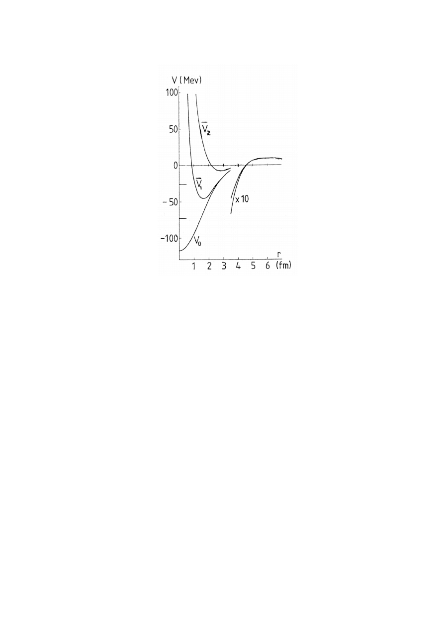
FIGURE 8.

Singular

potentials for l = 0 generated from the deep potential V

of Buck, Friedrich

and Wheatley [52] by the successive elimination of the two unphysical bound states of V

. ¯

is phase

equivalent to V

and ¯

. The removed bound states are represented by horizontal bars.

Sparenberg and Baye have used this approach to invert the experimental phase shifts of
neutron-proton elastic scattering in the

state to obtain singular potential with

= 1.

Andrianov, Borisov and Ioffe [59] have investigated the possibility of a supersymmetric
description of two half-integer spin particles by studying the supersymmetric aspect of
NN and N ¯

N scattering in the one-pion exchange approximation. Andrianov, Cannata,

Ioffe and Nishanidze [60] have studied matrix Hamiltonians using a SUSY approach
to hidden symmetries and have analysed coupled channel problems using this approach.
Sparenberg and Baye [61] have used SUSYQM to find coupled-channel potentials which
are phase equivalent and have removed the non-physical state of the deep

neutron-proton Moscow potential and transformed it into a shallow potential with a
repulsive core. There are many other examples of such applications of singular potentials
in Nuclear Physics.

7. CONCLUSIONS

In this course of lectures we have shown that starting from the simple idea of factorising
second order differential equations of a single variable it is possible to find a related
differential equation whose solutions are closely related to those of the original equation.

The relationship between the spectra and eigenfunctions of the two differential operators
are similar to those between the components of a supersymmetric doublet. The flexibility
available in the choice of factorization enables the manipulation of the spectrum of the
operators in desired fashion. We have shown that using the factorization method it is
possible to add or remove bound states or maintain the same spectrum but alter the
normalization constants of the eigenfunctions.

We have used these ideas to study the radial Schrödinger equation in detail. If the po-

tential of interaction is known then it is possible to find the eigenvalue spectrum, eigen-
functions and the phase shifts for positive energies by solving the radial Schrödinger
equation for a given partial wave. But if the potential of interaction is not known ac-
curately from first principles then one must use the spectral data like phase shifts and
energy levels to work backwards to find the potential. This is the subject of study of
inverse scattering theory. To determine the potential uniquely all the energy levels, the
normalization constants associated with the eigenfunctions of all the energy levels and
the phase shifts at all positive energies from 0 to

∞

must be known. Such a complete list

of data seldom exists and often phenomenological potentials with widely differing prop-
erties in terms of their behaviour as a function of r are used. In these lectures we have
shown that the concept of supersymmetric pairing enables the construction of inverse
scattering theory from some basic building blocks. We have shown that it is possible
to construct families of potentials with related phase shifts and other spectral proper-
ties. Such constructions have enabled the establishment of links between potentials with
startlingly dissimilar structure which nevertheless have closely related spectral proper-
ties. Even though the same properties could be found from the usual methods of inverse
scattering theory based on Gelfand-Levitan and Marchenko equations the method based
on the methods of SUSYQM has a particular simplicity and economy of expression and
opens up the possibility of similar constructions for other inverse problems arising in
other contexts. The method based on the supersymmetric construction has now been
extended to the study of coupled differential equations which has proved useful in the
study of a variety of coupled-channel problems in Nuclear Physics.

We have shown that the concept of supersymmetric pairing may be used to elucidate

the spectrum of the Dirac equation for an attractive Coulomb potential. We have also
shown that the Backlund transformation which provides a link between the N and N + 1
soliton solutions of the KdV hierarchy of non-linear differential equations is closely
related to a supersymmetric transformation which links the potential V

with N bound

states to another potential V

N+1

which has an additional bound state below the ground

state of V

The construction of singular potentials using suitable pairs of supersymmetric trans-

formations and their success in elucidating the relationship between diffferent model
potentials in Nuclear Physics is an outstanding example of the usefulness of SUSYQM
in a real physical context.

REFERENCES

J. Wess and B. Zumino, Nucl. Phys. B 70, 39 (1974).

A. Salam and J. Strathdee, Phys. Rev. D 11, 1521 (1975).

E. Witten, Nucl. Phys. B 188, 513 (1981).

G. Darboux, Compt. Rend. Acad. Sc. 94, 1456 (1882).

E. Schrödinger, Proc. Roy. Irish. Acad. A 46, 9, 183 (1940); 47, 53 (1941).

L. Infeld and T.E. Hull, Rev. Mod. Phys. 23, 21 (1951).

B. Freedman and F. Cooper, Ann. Phys. (N.Y.) 146, 262 (1983).

L.E. Gendenshtein, Sov. Phys. JETP Lett. 38, 356 (1983).

E. Gozzi, Phys. Lett. B 129, 432 (1983).

10. H. Ui, Prog. Theor. Phys. 72, 813 (1984).
11. H. Yamagishi, Phys. Rev. D 29, 2975 (1984).
12. V.A. Kostelecky and M.M. Nieto, Phys. Rev. Lett. 53, 2285 (1984).
13. B. Mielnik, J. Math. Phys. 25, 3387 (1984).
14. D.J. Fernández, Lett. Math. Phys. 8, 337 (1984).
15. M. Bernstein and L.S. Brown, Phys. Rev. Lett. 52, 1933 (1984).
16. A.A. Andrianov, N.V. Borisov and M.V. Ioffe, Phys. Lett. A 105, 19 (1984).
17. C.V. Sukumar, J. Phys. A: Math. Gen. 18, L57 (1985).
18. C.V. Sukumar, J.Phys. A: Math. Gen. 18 2917 (1985).
19. A.A. Andrianov, N.V. Borisov and M.V. Ioffe, Sov. J. Theor. Math. Phys. 70, 102 (1987).
20. P. Morse and H. Feshbach, Methods of Theoretical Physics: vol 1, McGraw-Hill, New York, 1953,

p768.

21. C.V. Sukumar, J. Phys. A: Math. Gen. 20, 2461 (1987).
22. V. Bargmann, Phys. Rev. 75, 301 (1949).
23. M. Abramowitz and I.A. Stegun, Handbook of Mathematical Functions, Dover, New York, 1965,

pp686.

24. I.M. Gelfand and B.M. Levitan, Am. Math. Soc. Transl. Ser. 2 1, 253 (1955).
25. V.A. Marchenko, Dokl. Akad. Nauk SSSR 104, 695 (1955).
26. P.B. Abraham and H.E. Moses, Phys. Rev. A 22, 133 (1980).
27. M.M. Nieto, Phys. Lett. B 145, 208 (1984).
28. C.V. Sukumar, J. Phys. A: Math. Gen. 18, 2937 (1985).
29. R.G. Newton, The Complex J-plane, Benjamin, New York, 1964, p14, p21, p30.
30. K. Chadan and P.C. Sabatier, Inverse Problems in Quantum Scattering Theory Springer, Berlin, 1977,

p25, p29, p55.

31. I.S. Gradshteyn and I.M. Ryzhik, Table of Integrals, Series and Products Academic Press, New York,

1965, p509.

32. J.D. Bjorken and S.D. Drell, Relativistic Quantum Mechanics, McGraw Hill, New York, 1964, p52.
33. C.V. Sukumar, J. Phys. A: Math. Gen. 18, L697 (1985).
34. C.G. Darwin, Proc. Roy. Soc. A 118, 654 (1928).
35. L.C. Biedenharn, Found. Phys. 13, 13 (1983).
36. C.V. Sukumar, J. Phys. A: Math. Gen. 19, 2297 (1986).
37. I. Kay and H.E. Moses, J. Appl. Phys. 27, 1503 (1956).
38. D.J. Korteweg and G.de Vries, Phil. Mag. 39, 422 (1895).
39. C.S. Gardner, J.M. Greene, M.D. Kruskal and R.M. Miura, Phys. Rev. Lett. 19, 1095 (1967).
40. A.C. Scott, F.Y.E. Chu and D.W. Mclaughlin, Proc. I.E.E.E. 61, 1443 (1973).
41. P.J. Caudrey, R.K. Dodd and J.D. Gibbon, Proc. Roy. Soc. Lon. A 351, 407 (1976).
42. C.V.Sukumar, in Proceedings of the Third International Colloquium on Differential Equations,

Plovdiv, VSP, Amsterdam, 1993, p167.

43. K. Sawada and T. Kotera, Prog. Theor. Phys. 51, 1355 (1974).
44. A.V. Backlund, Math. Ann. 9, 297 (1876); 19, 387 (1882).
45. H.B. Thacker, C. Quigg and J.L. Rosner, Phys. Rev. D 18 274, 287 (1978).
46. C. Quigg and J.L. Rosner, Phys. Rev. D 23, 2625 (1981).
47. K. Kwong and J.L. Rosner, Prog. Theor. phys. Suppl. 86, 366 (1986).
48. D. Baye, J. Phys. A: Math. Gen. 20, 5529 (1987).
49. P. Swan, Proc. Roy. Soc. London, A 228, 10 (1955).
50. P.Swan, Ann. Phys. (N.Y.) 48, 455 (1968).
51. P.Swan, Nucl. Phys. 46, 669 (1963).
52. B. Buck, H. Friedrich and C. Wheatley, Nucl. Phys. A 275, 246 (1977).

53. F. Michel, J. Albinski, P. Belery, T. Delbar, G. Gregoire, B. Tasiaux and G. Reidemeister, Phys. Rev.

C 28, 1904 (1983).

54. F. Michel and R. Vanderpoorten, Phys. Lett. B 82, 183 (1979).
55. S. Ali and A.R. Bodmer, Nucl. Phys. 80, 99 (1966).
56. F. Michel and G. Reidemeister, J. Phys. G 11, 835 (1985).
57. D. Baye, Phys. Rev. Lett. 58, 2738 (1987).
58. J.M. Sparenberg and D. Baye, Phys. Rev. C 55, 2175 (1997).
59. A.A. Andrianov, N.V. Borisov and M.V. Ioffe, Sov. J. Theor. Math. Phys. 72,748 (1987).
60. A.A. Andrianov, F. Cannata, M.V. Ioffe and D.N. Nishnianidze, J. Phys. A: Math. Gen. 30, 5037

(1997).

61. J.M. Sparenberg and D. Baye, Phys. Rev. Lett. 79, 3802 (1997).

Wyszukiwarka

Podobne podstrony:
Decoherence, the Measurement Problem, and Interpretations of Quantum Mechanics 0312059
Curcumin improves learning and memory ability and its neuroprotective mechanism in mice
Seahra The Classical and Quantum Mechanics of
Magnetic Treatment of Water and its application to agriculture
Analysis of soil fertility and its anomalies using an objective model
53 755 765 Effect of Microstructural Homogenity on Mechanical and Thermal Fatique
Changes in passive ankle stiffness and its effects on gait function in
Extract from Armoracia rusticana and Its Flavonoid Components
[38]QUERCETIN AND ITS DERIVATIVES CHEMICAL STRUCTURE AND BIOACTIVITY – A REVIEW
Screw mechanisms and joints
Angielski tematy Performance appraisal and its role in business 1
conceptual storage in bilinguals and its?fects on creativi
Motivation and its influence on language learning
Pain following stroke, initially and at 3 and 18 months after stroke, and its association with other
The Vietnam Conflict and its?fects
International Law How it is Implemented and its?fects
Central Bank and its Role in Fi Nieznany

więcej podobnych podstron