arXiv:1404.6699v1 [cs.CR] 27 Apr 2014

An Argumentation-Based Framework to Address the

Attribution Problem in Cyber-Warfare

Paulo Shakarian

1

Gerardo I. Simari

2

Geoffrey Moores

1

Simon Parsons

3

Marcelo A. Falappa

4

1

Dept. of Electrical Engineering and Computer Science, U.S. Military Academy, West Point, NY

2

Dept. of Computer Science, University of Oxford, Oxford, UK

3

Dept. of Computer Science, University of Liverpool, Liverpool, UK

4

Dep. de Cs. e Ing. de la Computaci´

on, Univ. Nac. del Sur, Bah´ıa Blanca, Argentina and CONICET

[e-mail], [e-mail], [e-mail]

[e-mail], [e-mail]

Abstract

Attributing a cyber-operation through the use of mul-
tiple pieces of technical evidence (i.e., malware reverse-
engineering and source tracking) and conventional intelli-
gence sources (i.e., human or signals intelligence) is a diffi-
cult problem not only due to the effort required to obtain
evidence, but the ease with which an adversary can plant
false evidence. In this paper, we introduce a formal reason-
ing system called the InCA (Intelligent Cyber Attribution)
framework that is designed to aid an analyst in the attri-
bution of a cyber-operation even when the available infor-
mation is conflicting and/or uncertain. Our approach com-
bines argumentation-based reasoning, logic programming,
and probabilistic models to not only attribute an operation
but also explain to the analyst why the system reaches its
conclusions.

1

Introduction

An important issue in cyber-warfare is the puzzle of deter-
mining who was responsible for a given cyber-operation –
be it an incident of attack, reconnaissance, or information
theft. This is known as the “attribution problem” [1]. The
difficulty of this problem stems not only from the amount of
effort required to find forensic clues but also the ease with
which an attacker can plant false clues to mislead security
personnel. Further, while techniques such as forensics and
reverse-engineering [2], source tracking [3], honeypots [4],
and sinkholing [5] are commonly employed to find evidence
that can lead to attribution, it is unclear how this evidence
is to be combined and reasoned about. In a military setting,
such evidence is augmented with normal intelligence collec-
tion, such as human intelligence (HUMINT), signals intel-
ligence (SIGINT) and other means – this adds additional
complications to the task of attributing a given operation.
Essentially, cyber-attribution is a highly-technical intelli-
gence analysis problem where an analyst must consider a
variety of sources, each with its associated level of confi-
dence, to provide a decision maker (e.g., a military com-
mander) insight into who conducted a given operation.

As it is well known that people’s ability to conduct intel-

ligence analysis is limited [6], and due to the highly tech-
nical nature of many cyber evidence-gathering techniques,
an automated reasoning system would be best suited for
the task. Such a system must be able to accomplish sev-

eral goals, among which we distinguish the following main
capabilities:

1. Reason about evidence in a formal, principled manner,

i.e., relying on strong mathematical foundations.

2. Consider evidence for cyber attribution associated with

some level of probabilistic uncertainty.

3. Consider logical rules that allow for the system to draw

conclusions based on certain pieces of evidence and it-
eratively apply such rules.

4. Consider pieces of information that may not be com-

patible with each other, decide which information is
most relevant, and express why.

5. Attribute a given cyber-operation based on the above-

described features and provide the analyst with the
ability to understand how the system arrived at that
conclusion.

In this paper we present the InCA (Intelligent Cyber At-

tribution) framework, which meets all of the above qualities.
Our approach relies on several techniques from the artifi-
cial intelligence community, including argumentation, logic
programming, and probabilistic reasoning. We first out-
line the underlying mathematical framework and provide
examples based on real-world cases of cyber-attribution (cf.
Section 2); then, in Sections 3 and 4, we formally present
InCA and attribution queries, respectively. Finally, we dis-
cuss conclusions and future work in Section 5.

2

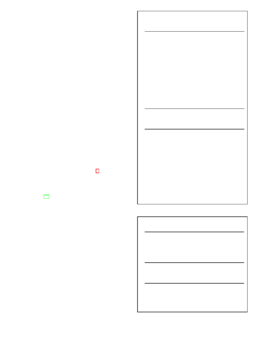
Two Kinds of Models

Our approach relies on two separate models of the world.
The first, called the environmental model (EM) is used
to describe the background knowledge and is probabilistic in
nature. The second one, called the analytical model (AM)
is used to analyze competing hypotheses that can account
for a given phenomenon (in this case, a cyber-operation).
The EM must be consistent – this simply means that there
must exist a probability distribution over the possible states
of the world that satisfies all of the constraints in the model,
as well as the axioms of probability theory. On the contrary,
the AM will allow for contradictory information as the sys-
tem must have the capability to reason about competing
explanations for a given cyber-operation. In general, the

EM

AM

“Malware X was compiled

“Malware X was compiled

on a system using the

on a system in English-

English language.”

speaking country Y.”

“Malware W and malware X

“Malware W and

were created in a similar

malware X are

coding style.”

related.”

“Country Y and country Z

“Country Y has a motive to

are currently at war.”

launch a cyber-attack against
country Z.”

“Country Y has a significant

“Country Y has the capability

investment in math-science-

to conduct a cyber-attack.”

engineering (MSE) education.”

Figure 1: Example observations – EM vs. AM.

EM contains knowledge such as evidence, intelligence re-
porting, or knowledge about actors, software, and systems.
The AM, on the other hand, contains ideas the analyst con-
cludes based on the information in the EM. Figure 1 gives
some examples of the types of information in the two mod-
els. Note that an analyst (or automated system) could as-
sign a probability to statements in the EM column whereas
statements in the AM column can be true or false depending
on a certain combination (or several possible combinations)
of statements from the EM. We now formally describe these
two models as well as a technique for annotating knowledge
in the AM with information from the EM – these annota-
tions specify the conditions under which the various state-
ments in the AM can potentially be true.

Before describing the two models in detail, we first in-

troduce the language used to describe them. Variable and
constant symbols represent items such as computer systems,
types of cyber operations, actors (e.g., nation states, hack-
ing groups), and other technical and/or intelligence infor-
mation. The set of all variable symbols is denoted with
V

, and the set of all constants is denoted with C. For our

framework, we shall require two subsets of C, C

act

and C

ops

,

that specify the actors that could conduct cyber-operations
and the operations themselves, respectively. In the exam-
ples in this paper, we will use capital letters to represent
variables (e.g., X, Y, Z). The constants in C

act

and C

ops

that we use in the running example are specified in the fol-
lowing example.

Example 2.1 The following (fictitious) actors and cyber-
operations will be used in our examples:

C

act

=

{baja, krasnovia, mojave}

(1)

C

ops

=

{worm123 }

(2)

The next component in the model is a set of predicate

symbols. These constructs can accept zero or more vari-
ables or constants as arguments, and map to either true
or false. Note that the EM and AM use separate sets of
predicate symbols – however, they can share variables and
constants. The sets of predicates for the EM and AM are
denoted with P

EM

, P

AM

, respectively. In InCA, we require

P

AM

to include the binary predicate condOp(X, Y ), where

X

is an actor and Y is a cyber-operation. Intuitively, this

means that actor X conducted operation Y . For instance,

condOp(baja, worm123 ) is true if baja was responsible for
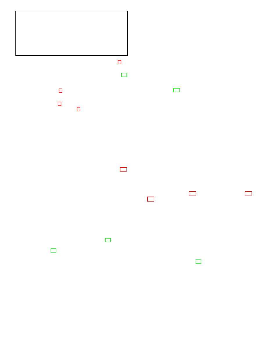
cyber-operation worm123 . A sample set of predicate sym-
bols for the analysis of a cyber attack between two states
over contention of a particular industry is shown in Figure 2;
these will be used in examples throughout the paper.

A construct formed with a predicate and constants as

arguments is known as a ground atom (we shall often deal
with ground atoms). The sets of all ground atoms for EM
and AM are denoted with G

EM

and G

AM

, respectively.

Example 2.2 The following are examples of ground atoms
over the predicates given in Figure 2.

G

EM

:

origIP (mw123sam1 , krasnovia),

mwHint (mw123sam1 , krasnovia),
inLgConf (krasnovia, baja),

mseTT (krasnovia, 2)

G

AM

:

evidOf (mojave, worm123 ),

motiv (baja, krasnovia),
expCw (baja),

tgt (krasnovia, worm123 )

For a given set of ground atoms, a world is a subset of the
atoms that are considered to be true (ground atoms not in
the world are false). Hence, there are 2

|G

EM

|

possible worlds

in the EM and 2

|G

AM

|

worlds in the AM, denoted with W

EM

and W

AM

, respectively.

Clearly, even a moderate number of ground atoms can

yield an enormous number of worlds to explore. One way
to reduce the number of worlds is to include integrity con-
straints, which allow us to eliminate certain worlds from
consideration – they simply are not possible in the setting
being modeled. Our principle integrity constraint will be of
the form:

oneOf

(A

′

)

where A

′

is a subset of ground atoms. Intuitively, this says

that any world where more than one of the atoms from
set A

′

appear is invalid. Let IC

EM

and IC

AM

be the sets

of integrity constraints for the EM and AM, respectively,
and the sets of worlds that conform to these constraints be
W

EM

(IC

EM

), W

AM

(IC

AM

), respectively.

Atoms can also be combined into formulas using standard

logical connectives: conjunction (and), disjunction (or), and
negation (not). These are written using the symbols ∧, ∨, ¬,
respectively. We say a world (w) satisfies a formula (f ),
written w |= f , based on the following inductive definition:

• if f is a single atom, then w |= f iff f ∈ w;

• if f = ¬f

′

then w |= f iff w 6|= f

′

;

• if f = f

′

∧ f

′′

then w |= f iff w |= f

′

and w |= f

′′

; and

• if f = f

′

∨ f

′′

then w |= f iff w |= f

′

or w |= f

′′

.

We use the notation f ormula

EM

, f ormula

AM

to denote the

set of all possible (ground) formulas in the EM and AM,
respectively. Also, note that we use the notation ⊤, ⊥ to

P

EM

:

origIP (M, X)

Malware M originated from an IP address belonging to actor X.

malwInOp(M, O)

Malware M was used in cyber-operation O.

mwHint(M, X)

Malware M contained a hint that it was created by actor X.

compilLang (M, C)

Malware M was compiled in a system that used language C.

nativLang(X, C)

Language C is the native language of actor X.

inLgConf (X, X

′

)

Actors X and X

′

are in a larger conflict with each other.

mseTT (X, N )

There are at least N number of top-tier math-science-engineering universities in country X.

infGovSys(X, M )

Systems belonging to actor X were infected with malware M .

cybCapAge(X, N )

Actor X has had a cyber-warfare capability for N years or less.

govCybLab(X)

Actor X has a government cyber-security lab.

P

AM

:

condOp(X, O)

Actor X conducted cyber-operation O.

evidOf (X, O)

There is evidence that actor X conducted cyber-operation O.

motiv (X, X

′

)

Actor X had a motive to launch a cyber-attack against actor X

′

.

isCap(X, O)

Actor X is capable of conducting cyber-operation O.

tgt(X, O)

Actor X was the target of cyber-operation O.

hasMseInvest (X)

Actor X has a significant investment in math-science-engineering education.

expCw (X)

Actor X has experience in conducting cyber-operations.

Figure 2: Predicate definitions for the environment and analytical models in the running example.

represent tautologies (formulas that are true in all worlds)
and contradictions (formulas that are false in all worlds),
respectively.

2.1

Environmental Model

In this section we describe the first of the two models,
namely the EM or environmental model. This model is
largely based on the probabilistic logic of [7], which we now
briefly review.

First, we define a probabilistic formula that consists of a

formula f over atoms from G

EM

, a real number p in the

interval [0, 1], and an error tolerance ǫ ∈ [0, min(p, 1 − p)].
A probabilistic formula is written as: f : p ± ǫ. Intuitively,
this statement is interpreted as “formula f is true with prob-
ability between p − ǫ and p + ǫ” – note that we make no
statement about the probability distribution over this inter-
val. The uncertainty regarding the probability values stems
from the fact that certain assumptions (such as probabilis-
tic independence) may not be suitable in the environment
being modeled.

Example 2.3 To continue our running example, consider
the following set Π

EM

:

f

1

=

govCybLab(baja) : 0.8 ± 0.1

f

2

=

cybCapAge(baja, 5) : 0.2 ± 0.1

f

3

=

mseTT (baja, 2) : 0.8 ± 0.1

f

4

=

mwHint(mw123sam1 , mojave)

∧ compilLang (worm123 , english) : 0.7 ± 0.2

f

5

=

malwInOp(mw123sam1 , worm123 )

∧ malwareRel (mw123sam1 , mw123sam2 )
∧ mwHint(mw123sam2 , mojave) : 0.6 ± 0.1

f

6

=

inLgConf (baja, krasnovia)

∨ ¬cooper (baja, krasnovia) : 0.9 ± 0.1

f

7

=

origIP (mw123sam1 , baja) : 1 ± 0

Throughout the paper, let Π

′

EM

= {f

1

, f

2

, f

3

}.

We now consider a probability distribution Pr over the

set W

EM

(IC

EM

).

We say that Pr satisfies probabilis-

tic formula f : p ± ǫ iff the following holds: p − ǫ ≤
P

w∈W

EM

(IC

EM

)

Pr (w) ≤ p + ǫ. A set Π

EM

of probabilistic

formulas is called a knowledge base. We say that a prob-
ability distribution over W

EM

(IC

EM

) satisfies Π

EM

if and

only if it satisfies all probabilistic formulas in Π

EM

.

It is possible to create probabilistic knowledge bases for

which there is no satisfying probability distribution. The
following is a simple example of this:

condOp(krasnovia, worm123 )

∨ condOp(baja, worm123 ) : 0.4 ± 0;

condOp(krasnovia, worm123 )

∧ condOp(baja, worm123 ) : 0.6 ± 0.1.

Formulas and knowledge bases of this sort are inconsis-

tent. In this paper, we assume that information is properly
extracted from a set of historic data and hence consistent;
(recall that inconsistent information can only be handled in
the AM, not the EM). A consistent knowledge base could
also be obtained as a result of curation by experts, such that
all inconsistencies were removed – see [8, 9] for algorithms
for learning rules of this type.

The main kind of query that we require for the proba-

bilistic model is the maximum entailment problem: given
a knowledge base Π

EM

and a (non-probabilistic) formula

q

, identify p, ǫ such that all valid probability distributions

Pr that satisfy Π

EM

also satisfy q : p ± ǫ, and there does

not exist p

′

, ǫ

′

s.t. [p − ǫ, p + ǫ] ⊃ [p

′

− ǫ

′

, p

′

+ ǫ

′

], where

all probability distributions Pr that satisfy Π

EM

also sat-

isfy q : p

′

± ǫ

′

. That is, given q, can we determine the

probability (with maximum tolerance) of statement q given
the information in Π

EM

? The approach adopted in [7] to

solve this problem works as follows. First, we must solve
the linear program defined next.

Definition 2.1 (EM-LP-MIN) Given a knowledge base
Π

EM

and a formula q:

• create a variable x

i

for each w

i

∈ W

EM

(IC

EM

);

• for each f

j

: p

j

± ǫ

j

∈ Π

EM

, create constraint:

p

j

− ǫ

j

≤

X

w

i

∈W

EM

(IC

EM

) s.t. w

i

|=f

j

x

i

≤ p

j

+ ǫ

j

;

• finally, we also have a constraint:

X

w

i

∈W

EM

(IC

EM

)

x

i

= 1.

The objective is to minimize the function:

X

w

i

∈W

EM

(IC

EM

) s.t. w

i

|=q

x

i

.

We use the notation EP-LP-MIN(Π

EM

, q

) to refer to the

value of the objective function in the solution to the EM-
LP-MIN constraints.

Let ℓ be the result of the process described in Defini-

tion 2.1. The next step is to solve the linear program a
second time, but instead maximizing the objective function
(we shall refer to this as EM-LP-MAX) – let u be the re-
sult of this operation. In [7], it is shown that ǫ =

u−ℓ

2

and

p

= ℓ + ǫ is the solution to the maximum entailment prob-

lem. We note that although the above linear program has an
exponential number of variables in the worst case (i.e., no
integrity constraints), the presence of constraints has the
potential to greatly reduce this space. Further, there are
also good heuristics (cf. [8, 10]) that have been shown to
provide highly accurate approximations with a reduced-size
linear program.

Example 2.4 Consider KB Π

′

EM

from Example 2.3 and a

set of ground atoms restricted to those that appear in that
program. Hence, we have:

w

1

= {govCybLab(baja), cybCapAge(baja, 5),

mseTT (baja, 2)}

w

2

= {govCybLab(baja), cybCapAge(baja, 5)}

w

3

= {govCybLab(baja), mseTT (baja, 2)}

w

4

= {cybCapAge(baja, 5), mseTT (baja, 2)}

w

5

= {cybCapAge(baja, 5)}

w

6

= {govCybLab(baja)}

w

7

= {mseTT (baja, 2)}

w

8

= ∅

and suppose we wish to compute the probability for formula:

q

= govCybLab(baja) ∨ mseTT (baja, 2).

For each formula in Π

EM

we have a constraint, and for

each world above we have a variable. An objective function
is created based on the worlds that satisfy the query formula
(here, worlds w

1

–w

4

, w

6

, w

7

). Hence, EP-LP-MIN(Π

′

EM

, q

)

can be written as:

max

x

1

+ x

2

+ x

3

+ x

4

+ x

6

+ x

7

w .r .t . :

0.7 ≤

x

1

+ x

2

+ x

3

+ x

6

≤ 0.9

0.1 ≤

x

1

+ x

2

+ x

4

+ x

5

≤ 0.3

0.8 ≤

x

1

+ x

3

+ x

4

+ x

7

≤ 1

x

1

+ x

2

+ x

3

+ x

4

+ x

5

+ x

6

+ x

7

+ x

8

= 1

We

can

now

solve

EP-LP-MAX(Π

′

EM

, q

)

and

EP-LP-MIN(Π

′

EM

, q

) to get solution 0.9 ± 0.1.

2.2

Analytical Model

For the analytical model (AM), we choose a structured argu-
mentation framework [11] due to several characteristics that
make such frameworks highly applicable to cyber-warfare
domains. Unlike the EM, which describes probabilistic in-
formation about the state of the real world, the AM must
allow for competing ideas – it must be able to represent
contradictory information. The algorithmic approach al-
lows for the creation of arguments based on the AM that
may “compete” with each other to describe who conducted
a given cyber-operation. In this competition – known as a
dialectical process – one argument may defeat another based
on a comparison criterion that determines the prevailing ar-
gument. Resulting from this process, the InCA framework
will determine arguments that are warranted (those that
are not defeated by other arguments) thereby providing a
suitable explanation for a given cyber-operation.

The transparency provided by the system can allow ana-

lysts to identify potentially incorrect input information and
fine-tune the models or, alternatively, collect more infor-
mation. In short, argumentation-based reasoning has been
studied as a natural way to manage a set of inconsistent in-
formation – it is the way humans settle disputes. As we will
see, another desirable characteristic of (structured) argu-
mentation frameworks is that, once a conclusion is reached,
we are left with an explanation of how we arrived at it
and information about why a given argument is warranted;
this is very important information for analysts to have. In
this section, we recall some preliminaries of the underly-
ing argumentation framework used, and then introduce the
analytical model (AM).

Defeasible Logic Programming with Presumptions

DeLP with Presumptions (PreDeLP) [12] is a formalism
combining Logic Programming with Defeasible Argumen-
tation. We now briefly recall the basics of PreDeLP; we
refer the reader to [13, 12] for the complete presentation.
The formalism contains several different constructs: facts,
presumptions, strict rules, and defeasible rules. Facts are
statements about the analysis that can always be consid-
ered to be true, while presumptions are statements that
may or may not be true. Strict rules specify logical con-
sequences of a set of facts or presumptions (similar to an
implication, though not the same) that must always occur,
while defeasible rules specify logical consequences that may
be assumed to be true when no contradicting information
is present. These constructs are used in the construction
of arguments, and are part of a PreDeLP program, which
is a set of facts, strict rules, presumptions, and defeasible
rules. Formally, we use the notation Π

AM

= (Θ, Ω, Φ, ∆)

to denote a PreDeLP program, where Ω is the set of strict
rules, Θ is the set of facts, ∆ is the set of defeasible rules,
and Φ is the set of presumptions. In Figure 3, we provide
an example Π

AM

. We now describe each of these constructs

in detail.

Facts (Θ) are ground literals representing atomic informa-
tion or its negation, using strong negation “¬”. Note that
all of the literals in our framework must be formed with a
predicate from the set P

AM

. Note that information in this

form cannot be contradicted.

Strict Rules (Ω) represent non-defeasible cause-and-effect
information that resembles an implication (though the se-
mantics is different since the contrapositive does not hold)
and are of the form L

0

← L

1

, . . . , L

n

, where L

0

is a ground

literal and {L

i

}

i>0

is a set of ground literals.

Presumptions (Φ) are ground literals of the same form as
facts, except that they are not taken as being true but rather
defeasible, which means that they can be contradicted. Pre-
sumptions are denoted in the same manner as facts, except
that the symbol

–≺

is added. While any literal can be used

as a presumption in InCA, we specifically require all literals
created with the predicate condOp to be defeasible.

Defeasible Rules (∆) represent tentative knowledge that
can be used if nothing can be posed against it. Just as pre-
sumptions are the defeasible counterpart of facts, defeasible
rules are the defeasible counterpart of strict rules. They
are of the form L

0

–≺

L

1

, . . . , L

n

, where L

0

is a ground lit-

eral and {L

i

}

i>0

is a set of ground literals. Note that with

both strict and defeasible rules, strong negation is allowed
in the head of rules, and hence may be used to represent
contradictory knowledge.

Even though the above constructs are ground, we allow

for schematic versions with variables that are used to repre-
sent sets of ground rules. We denote variables with strings
starting with an uppercase letter; Figure 4 shows a non-
ground example.

When a cyber-operation occurs, InCA must derive ar-

guments as to who could have potentially conducted the
action. Derivation follows the same mechanism of Logic
Programming [14].

Since rule heads can contain strong

negation, it is possible to defeasibly derive contradictory
literals from a program. For the treatment of contradictory
knowledge, PreDeLP incorporates a defeasible argumenta-
tion formalism that allows the identification of the pieces of
knowledge that are in conflict, and through the previously
mentioned dialectical process decides which information pre-
vails as warranted.

This dialectical process involves the construction and

evaluation of arguments that either support or interfere
with a given query, building a dialectical tree in the pro-
cess. Formally, we have:

Definition 2.2 (Argument) An argument hA, Li for a
literal L is a pair of the literal and a (possibly empty) set
of the EM (A ⊆ Π

AM

) that provides a minimal proof for L

meeting the requirements: (1.) L is defeasibly derived from
A, (2.) Ω ∪ Θ ∪ A is not contradictory, and (3.) A is a
minimal subset of ∆ ∪ Φ satisfying 1 and 2, denoted hA, Li.

Literal L is called the conclusion supported by the argu-

ment, and A is the support of the argument. An argument
hB, Li is a subargument of hA, L

′

i iff B ⊆ A. An argument

hA, Li is presumptive iff A ∩ Φ is not empty. We will also
use Ω(A) = A ∩ Ω, Θ(A) = A ∩ Θ, ∆(A) = A ∩ ∆, and
Φ(A) = A ∩ Φ.

Θ :

θ

1a

=

evidOf (baja, worm123 )

θ

1b

=

evidOf (mojave, worm123 )

θ

2

=

motiv (baja, krasnovia)

Ω :

ω

1a

=

¬condOp(baja, worm123 ) ←

condOp(mojave, worm123 )

ω

1b

=

¬condOp(mojave, worm123 ) ←

condOp(baja, worm123 )

ω

2a

=

condOp(baja, worm123 ) ←

evidOf (baja, worm123 ),
isCap(baja, worm123 ),
motiv (baja, krasnovia),
tgt(krasnovia, worm123 )

ω

2b

=

condOp(mojave, worm123 ) ←

evidOf (mojave, worm123 ),
isCap(mojave, worm123 ),
motiv (mojave, krasnovia),
tgt(krasnovia, worm123 )

Φ :

φ

1

=

hasMseInvest (baja)

–≺

φ

2

=

tgt (krasnovia, worm123 )

–≺

φ

3

=

¬expCw (baja)

–≺

∆ :

δ

1a

=

condOp(baja, worm123 )

–≺

evidOf (baja, worm123 )

δ

1b

=

condOp(mojave, worm123 )

–≺

evidOf (mojave, worm123 )

δ

2

=

condOp(baja, worm123 )

–≺

isCap(baja, worm123 )

δ

3

=

condOp(baja, worm123 )

–≺

motiv (baja, krasnovia),
tgt(krasnovia, worm123 )

δ

4

=

isCap(baja, worm123 )

–≺

hasMseInvest (baja)

δ

5a

=

¬isCap(baja, worm123 )

–≺

¬expCw (baja)

δ

5b

=

¬isCap(mojave, worm123 )

–≺

¬expCw (mojave)

Figure 3: A ground argumentation framework.

Θ :

θ

1

=

evidOf (baja, worm123 )

θ

2

=

motiv (baja, krasnovia)

Ω :

ω

1

=

¬condOp(X, O) ← condOp(X

′

, O

),

X

6= X

′

ω

2

=

condOp(X, O) ← evidOf (X, O),

isCap(X, O), motiv (X, X

′

),

tgt(X

′

, O

), X 6= X

′

Φ :

φ

1

=

hasMseInvest (baja)

–≺

φ

2

=

tgt (krasnovia, worm123 )

–≺

φ

3

=

¬expCw (baja)

–≺

∆ :

δ

1

=

condOp(X, O)

–≺

evidOf (X, O)

δ

2

=

condOp(X, O)

–≺

isCap(X, O)

δ

3

=

condOp(X, O)

–≺

motiv (X, X

′

), tgt(X

′

, O

)

δ

4

=

isCap(X, O)

–≺

hasMseInvest (X)

δ

5

=

¬isCap(X, O)

–≺

¬expCw (X)

Figure 4: A non-ground argumentation framework.

hA

1

,

condOp(baja, worm123 )i

A

1

= {θ

1a

, δ

1a

}

hA

2

,

condOp(baja, worm123 )i

A

2

= {φ

1

, φ

2

, δ

4

, ω

2a

,

θ

1a

, θ

2

}

hA

3

,

condOp(baja, worm123 )i

A

3

= {φ

1

, δ

2

, δ

4

}

hA

4

,

condOp(baja, worm123 )i

A

4

= {φ

2

, δ

3

, θ

2

}

hA

5

,

isCap(baja, worm123 )i

A

5

= {φ

1

, δ

4

}

hA

6

,

¬condOp(baja, worm123 )i

A

6

= {δ

1b

, θ

1b

, ω

1a

}

hA

7

,

¬isCap(baja, worm123 )i

A

7

= {φ

3

, δ

5a

}

Figure 5: Example ground arguments from Figure 3.

Note that our definition differs slightly from that of [15]

where DeLP is introduced, as we include strict rules and
facts as part of the argument. The reason for this will be-
come clear in Section 3. Arguments for our scenario are
shown in the following example.

Example 2.5 Figure 5 shows example arguments based on
the knowledge base from Figure 3. Note that the following
relationship exists:

hA

5

,

isCap(baja, worm123 )i is a sub-argument of

hA

2

,

condOp(baja, worm123 )i and

hA

3

,

condOp(baja, worm123 )i.

Given argument hA

1

, L

1

i, counter-arguments are argu-

ments that contradict it. Argument hA

2

, L

2

i counterargues

or attacks hA

1

, L

1

i literal L

′

iff there exists a subargument

hA, L

′′

i of hA

1

, L

1

i s.t. set Ω(A

1

)∪Ω(A

2

)∪Θ(A

1

)∪Θ(A

2

)∪

{L

2

, L

′′

} is contradictory.

Example 2.6 Consider the arguments from Example 2.5.
The following are some of the attack relationships between
them: A

1

, A

2

, A

3

, and A

4

all attack A

6

; A

5

attacks A

7

;

and A

7

attacks A

2

.

A proper defeater of an argument hA, Li is a counter-

argument that – by some criterion – is considered to be
better than hA, Li; if the two are incomparable according
to this criterion, the counterargument is said to be a block-
ing defeater. An important characteristic of PreDeLP is
that the argument comparison criterion is modular, and
thus the most appropriate criterion for the domain that
is being represented can be selected; the default criterion
used in classical defeasible logic programming (from which
PreDeLP is derived) is generalized specificity [16], though
an extension of this criterion is required for arguments us-
ing presumptions [12]. We briefly recall this criterion next
– the first definition is for generalized specificity, which is
subsequently used in the definition of presumption-enabled
specificity.

Definition 2.3 Let Π

AM

= (Θ, Ω, Φ, ∆) be a PreDeLP

program and let F be the set of all literals that have a defea-
sible derivation from Π

AM

. An argument hA

1

, L

1

i is pre-

ferred to hA

2

, L

2

i, denoted with A

1

≻

P S

A

2

iff the two

following conditions hold:

1. For all H ⊆ F, Ω(A

1

)∪Ω(A

2

)∪H is non-contradictory:

if there is a derivation for L

1

from Ω(A

2

) ∪ Ω(A

1

) ∪

∆(A

1

) ∪ H, and there is no derivation for L

1

from

Ω(A

1

) ∪ Ω(A

2

) ∪ H, then there is a derivation for L

2

from Ω(A

1

) ∪ Ω(A

2

) ∪ ∆(A

2

) ∪ H.

2. There is at least one set H

′

⊆ F, Ω(A

1

) ∪ Ω(A

2

) ∪

H

′

is non-contradictory, such that there is a derivation

for L

2

from Ω(A

1

) ∪ Ω(A

2

) ∪ H

′

∪ ∆(A

2

), there is no

derivation for L

2

from Ω(A

1

)∪Ω(A

2

)∪H

′

, and there is

no derivation for L

1

from Ω(A

1

)∪Ω(A

2

)∪H

′

∪∆(A

1

).

Intuitively, the principle of specificity says that, in the

presence of two conflicting lines of argument about a propo-
sition, the one that uses more of the available information is
more convincing. A classic example involves a bird, Tweety,
and arguments stating that it both flies (because it is a
bird) and doesn’t fly (because it is a penguin). The latter
argument uses more information about Tweety – it is more
specific – and is thus the stronger of the two.

Definition 2.4 ([12]) Let Π

AM

= (Θ, Ω, Φ, ∆) be a Pre-

DeLP program.

An argument hA

1

, L

1

i is preferred to

hA

2

, L

2

i, denoted with A

1

≻ A

2

iff any of the following

conditions hold:

1. hA

1

, L

1

i and hA

2

, L

2

i are both factual arguments and

hA

1

, L

1

i ≻

P S

hA

2

, L

2

i.

2. hA

1

, L

1

i is a factual argument and hA

2

, L

2

i is a pre-

sumptive argument.

3. hA

1

, L

1

i and hA

2

, L

2

i are presumptive arguments, and

(a) ¬(Φ(A

1

) ⊆ Φ(A

2

)), or

(b) Φ(A

1

) = Φ(A

2

) and hA

1

, L

1

i ≻

P S

hA

2

, L

2

i.

Generally, if A, B are arguments with rules X and Y , resp.,
and X ⊂ Y , then A is stronger than B. This also holds when
A and B use presumptions P

1

and P

2

, resp., and P

1

⊂ P

2

.

Example 2.7 The following are relationships between ar-
guments from Example 2.5, based on Definitions 2.3
and 2.4:
A

1

and A

6

are incomparable (blocking defeaters);

A

6

≻ A

2

, and thus A

6

defeats A

2

;

A

6

≻ A

3

, and thus A

6

defeats A

3

;

A

6

≻ A

4

, and thus A

6

defeats A

4

;

A

5

and A

7

are incomparable (blocking defeaters).

A sequence of arguments called an argumentation line

thus arises from this attack relation, where each argument
defeats its predecessor. To avoid undesirable sequences,
that may represent circular or fallacious argumentation
lines, in DeLP an argumentation line is acceptable if it sat-
isfies certain constraints (see [13]). A literal L is warranted
if there exists a non-defeated argument A supporting L.

Clearly, there can be more than one defeater for a par-

ticular argument hA, Li. Therefore, many acceptable argu-
mentation lines could arise from hA, Li, leading to a tree
structure. The tree is built from the set of all argumenta-
tion lines rooted in the initial argument. In a dialectical
tree, every node (except the root) represents a defeater of
its parent, and leaves correspond to undefeated arguments.
Each path from the root to a leaf corresponds to a different
acceptable argumentation line. A dialectical tree provides
a structure for considering all the possible acceptable argu-
mentation lines that can be generated for deciding whether

an argument is defeated. We call this tree dialectical be-
cause it represents an exhaustive dialectical

1

analysis for

the argument in its root. For argument hA, Li, we denote
its dialectical tree with T (h

A

, L

i).

Given a literal L and an argument hA, Li, in order to de-

cide whether or not a literal L is warranted, every node in
the dialectical tree T (h

A

, L

i) is recursively marked as “D”

(defeated ) or “U” (undefeated ), obtaining a marked dialec-
tical tree T

∗

(h

A

, L

i) where:

• All leaves in T

∗

(h

A

, L

i) are marked as “U”s, and

• Let hB, qi be an inner node of T

∗

(h

A

, L

i). Then, hB, qi

will be marked as “U” iff every child of hB, qi is marked
as “D”. Node hB, qi will be marked as “D” iff it has at
least a child marked as “U”.

Given argument hA, Li over Π

AM

, if the root of T

∗

(h

A

, L

i)

is marked “U”, then T

∗

(

hA, hi

) warrants L and that L is

warranted from Π

AM

. (Warranted arguments correspond to

those in the grounded extension of a Dung argumentation
system [17].)

We can then extend the idea of a dialectical tree to a

dialectical forest. For a given literal L, a dialectical forest
F(L) consists of the set of dialectical trees for all arguments
for L. We shall denote a marked dialectical forest, the set of
all marked dialectical trees for arguments for L, as F

∗

(L).

Hence, for a literal L, we say it is warranted if there is at
least one argument for that literal in the dialectical forest
F

∗

(L) that is labeled “U”, not warranted if there is at least

one argument for literal ¬L in the forest F

∗

(¬L) that is

labeled “U”, and undecided otherwise.

3

The InCA Framework

Having defined our environmental and analytical models
(Π

EM

,

Π

AM

respectively), we now define how the two re-

late, which allows us to complete the definition of our InCA
framework.

The key intuition here is that given a Π

AM

, every ele-

ment of Ω ∪ Θ ∪ ∆ ∪ Φ might only hold in certain worlds
in the set W

EM

– that is, worlds specified by the environ-

ment model. As formulas over the environmental atoms
in set G

EM

specify subsets of W

EM

(i.e., the worlds that

satisfy them), we can use these formulas to identify the
conditions under which a component of Ω ∪ Θ ∪ ∆ ∪ Φ can
be true. Recall that we use the notation f ormula

EM

to

denote the set of all possible formulas over G

EM

. There-

fore, it makes sense to associate elements of Ω ∪ Θ ∪ ∆ ∪ Φ
with a formula from f ormula

EM

. In doing so, we can in

turn compute the probabilities of subsets of Ω ∪ Θ ∪ ∆ ∪ Φ
using the information contained in Π

EM

, which we shall de-

scribe shortly. We first introduce the notion of annotation
function, which associates elements of Ω ∪ Θ ∪ ∆ ∪ Φ with
elements of f ormula

EM

.

We also note that, by using the annotation function (see

Figure 6), we may have certain statements that appear as
both facts and presumptions (likewise for strict and defea-
sible rules). However, these constructs would have differ-
ent annotations, and thus be applicable in different worlds.

1

In the sense of providing reasons for and against a position.

af (θ

1

) =

origIP (worm123 , baja)∨

malwInOp(worm123 , o)∧
mwHint (worm123 , baja)∨

(compilLang (worm123 , c)∧
nativLang(baja, c))

af (θ

2

) =

inLgConf (baja, krasnovia)

af (ω

1

) =

True

af (ω

2

) =

True

af (φ

1

) =

mseTT (baja, 2) ∨ govCybLab(baja)

af (φ

2

) =

malwInOp(worm123 , o

′

)∧

infGovSys(krasnovia , worm123 )

af (φ

3

) =

cybCapAge(baja, 5)

af (δ

1

) =

True

af (δ

2

) =

True

af (δ

3

) =

True

af (δ

4

) =

True

af (δ

5

) =

True

Figure 6: Example annotation function.

Suppose we added the following presumptions to our run-
ning example:

φ

3

= evidOf (X, O)

–≺

, and

φ

4

= motiv (X, X

′

)

–≺

.

Note that these presumptions are constructed using the
same formulas as facts θ

1

, θ

2

. Suppose we extend af as

follows:

af (φ

3

) =

malwInOp(M, O) ∧ malwareRel (M, M

′

)

∧mwHint(M

′

, X

)

af (φ

4

) =

inLgConf (Y, X

′

) ∧ cooper (X, Y )

So, for instance, unlike θ

1

, φ

3

can potentially be true in any

world of the form:

{malwInOp(M, O), malwareRel (M, M

′

), mwHint (M

′

, X

)}

while θ

1

cannot be considered in any those worlds.

With the annotation function, we now have all the com-

ponents to formally define an InCA framework.

Definition 3.1 (InCA Framework) Given environmen-
tal model Π

EM

, analytical model Π

AM

, and annotation

function af , I = (Π

EM

,

Π

AM

,

af ) is an InCA frame-

work

.

Given the setup described above, we consider a world-

based approach – the defeat relationship among arguments
will depend on the current state of the world (based on the
EM). Hence, we now define the status of an argument with
respect to a given world.

Definition 3.2 (Validity) Given InCA framework
I = (Π

EM

,

Π

AM

,

af ), argument hA, Li is valid w.r.t. world

w

∈ W

EM

iff ∀c ∈ A, w |= af (c).

In other words, an argument is valid with respect to w

if the rules, facts, and presumptions in that argument are

present in w – the argument can then be built from infor-
mation that is available in that world. In this paper, we
extend the notion of validity to argumentation lines, dialec-
tical trees, and dialectical forests in the expected way (an
argumentation line is valid w.r.t. w iff all arguments that
comprise that line are valid w.r.t. w).

Example 3.1 Consider worlds w

1

, . . . , w

8

from Exam-

ple 2.4 along with the argument hA

5

,

isCap(baja, worm123 )i

from Example 2.5. This argument is valid in worlds w

1

–w

4

,

w

6

, and w

7

.

We now extend the idea of a dialectical tree w.r.t.

worlds – so, for a given world w ∈ W

EM

, the dialectical

(resp., marked dialectical) tree induced by w is denoted
by T

w

hA, Li (resp., T

∗

w

hA, Li). We require that all argu-

ments and defeaters in these trees to be valid with respect
to w. Likewise, we extend the notion of dialectical forests in
the same manner (denoted with F

w

(L) and F

∗

w

(L), respec-

tively). Based on these concepts we introduce the notion
of warranting scenario.

Definition 3.3 (Warranting Scenario) Let I = (Π

EM

,

Π

AM

,

af ) be an InCA framework and L be a ground literal

over G

AM

; a world w ∈ W

EM

is said to be a warranting

scenario for L (denoted w ⊢

war

L

) iff there is a dialectical

forest F

∗

w

(L) in which L is warranted and F

∗

w

(L) is valid

w.r.t w.

Example 3.2 Following from Example 3.1, argument
hA

5

,

isCap(baja, worm123 )i is warranted in worlds w

3

, w

6

,

and w

7

.

Hence, the set of worlds in the EM where a literal L in the

AM must be true is exactly the set of warranting scenarios
– these are the “necessary” worlds, denoted:

nec

(L) = {w ∈ W

EM

| (w ⊢

war

L

).}

Now, the set of worlds in the EM where AM literal L can
be true is the following – these are the “possible” worlds,
denoted:

poss

(L) = {w ∈ W

EM

| w 6⊢

war

¬L}.

The following example illustrates these concepts.

Example 3.3 Following from Example 3.1:

nec

(isCap(baja, worm123 )) = {w

3

, w

6

, w

7

} and

poss

(isCap(baja, worm123 )) = {w

1

, w

2

, w

3

, w

4

, w

6

, w

7

}.

Hence, for a given InCA framework I, if we are given

a probability distribution Pr over the worlds in the EM,
then we can compute an upper and lower bound on the
probability of literal L (denoted P

L,Pr ,I

) as follows:

ℓ

L,Pr,I

=

X

w∈nec(L)

Pr (w),

u

L,Pr ,I

=

X

w∈poss(L)

Pr (w),

and

ℓ

L,Pr,I

≤ P

L,Pr ,I

≤ u

L,Pr,I

.

Now let us consider the computation of probability

bounds on a literal when we are given a knowledge base
Π

EM

in the environmental model, which is specified in I,

instead of a probability distribution over all worlds. For a
given world w ∈ W

EM

, let f or(w) =

V

a∈w

a

∧ V

a /

∈w

¬a

– that is, a formula that is satisfied only by world w. Now
we can determine the upper and lower bounds on the prob-
ability of a literal w.r.t. Π

EM

(denoted P

L,I

) as follows:

ℓ

L,I

= EP-LP-MIN





Π

EM

,

_

w∈nec(L)

f or

(w)





,

u

L,I

= EP-LP-MAX





Π

EM

,

_

w∈poss(L)

f or

(w)





,

and

ℓ

L,I

≤ P

L,I

≤ u

L,I

.

Hence, P

L,I

=

ℓ

L,I

+

u

L,I

−ℓ

L,I

2

±

u

L,I

−ℓ

L,I

2

.

Example 3.4 Following

from

Example

3.1,

argu-

ment

hA

5

,

isCap(baja, worm123 )i,

we

can

compute

P

isCap

(baja,worm123 ),I

(where I = (Π

′

EM

,

Π

AM

,

af )). Note

that for the upper bound, the linear program we need to set
up is as in Example 2.4. For the lower bound, the objective
function changes to: min x

3

+ x

6

+ x

7

. From these linear

constraints, we obtain: P

isCap

(baja,worm123 ),I

= 0.75 ± 0.25.

4

Attribution Queries

We now have the necessary elements required to formally
define the kind of queries that correspond to the attribution
problems studied in this paper.

Definition 4.1 Let I = (Π

EM

,

Π

AM

,

af ) be an InCA

framework, S ⊆ C

act

(the set of “suspects”), O ∈ C

ops

(the “operation”), and E ⊆ G

EM

(the “evidence”). An ac-

tor A ∈ S is said to be a most probable suspect iff there does
not exist A

′

∈ S such that P

condOp

(A

′

,O),I

′

> P

condOp

(A,O),I

′

where I

′

= (Π

EM

∪ Π

E

,

Π

AM

,

af

′

) with Π

E

defined as

S

c∈E

{c : 1 ± 0}.

Given the above definition, we refer to Q = (I, S, O, E)

as an attribution query, and A as an answer to Q. We note
that in the above definition, the items of evidence are added
to the environmental model with a probability of 1. While
in general this may be the case, there are often instances
in analysis of a cyber-operation where the evidence may be
true with some degree of uncertainty. Allowing for proba-
bilistic evidence is a simple extension to Definition 4.1 that
does not cause any changes to the results of this paper.

To understand how uncertain evidence can be present in

a cyber-security scenario, consider the following. In Syman-
tec’s initial analysis of the Stuxnet worm, they found the
routine designed to attack the S7-417 logic controller was

incomplete, and hence would not function [18]. However, in-
dustrial control system expert Ralph Langner claimed that
the incomplete code would run provided a missing data
block is generated, which he thought was possible [19]. In
this case, though the code was incomplete, there was clearly
uncertainty regarding its usability. This situation provides
a real-world example of the need to compare arguments –
in this case, in the worlds where both arguments are valid,
Langner’s argument would likely defeat Symantec’s by gen-
eralized specificity (the outcome, of course, will depend on
the exact formalization of the two). Note that Langner
was later vindicated by the discovery of an older sample,
Stuxnet 0.5, which generated the data block.

2

InCA also allows for a variety of relevant scenarios to the

attribution problem. For instance, we can easily allow for
the modeling of non-state actors by extending the available
constants – for example, traditional groups such as Hezbol-
lah, which has previously wielded its cyber-warfare capabil-
ities in operations against Israel [1]. Likewise, the InCA can
also be used to model cooperation among different actors
in performing an attack, including the relationship between
non-state actors and nation-states, such as the potential
connection between Iran and militants stealing UAV feeds in
Iraq, or the much-hypothesized relationship between hack-
tivist youth groups and the Russian government [1]. An-
other aspect that can be modeled is deception where, for
instance, an actor may leave false clues in a piece of mal-
ware to lead an analyst to believe a third party conducted
the operation. Such a deception scenario can be easily cre-
ated by adding additional rules in the AM that allow for
the creation of such counter-arguments. Another type of
deception that could occur include attacks being launched
from a system not in the responsible party’s area, but under
their control (e.g., see [5]). Again, modeling who controls a
given system can be easily accomplished in our framework,
and doing so would simply entail extending an argumenta-
tion line. Further, campaigns of cyber-operations can also
be modeled, as well as relationships among malware and/or
attacks (as detailed in [20]).

As with all of these abilities, InCA provides the analyst

the means to model a complex situation in cyber-warfare
but saves him from carrying out the reasoning associated
with such a situation. Additionally, InCA results are con-
structive, so an analyst can “trace-back” results to better
understand how the system arrived at a given conclusion.

5

Conclusion

In this paper we introduced InCA, a new framework that
allows the modeling of various cyber-warfare/cyber-security
scenarios in order to help answer the attribution question
by means of a combination of probabilistic modeling and ar-
gumentative reasoning. This is the first framework, to our
knowledge, that addresses the attribution problem while al-
lowing for multiple pieces of evidence from different sources,
including traditional (non-cyber) forms of intelligence such
as human intelligence. Further, our framework is the first

2

http://www.symantec.com/connect/blogs/stuxnet-05-disrupting-

uranium-processing-natanz

to extend Defeasible Logic Programming with probabilis-
tic information. Currently, we are implementing InCA and
the associated algorithms and heuristics to answer these
queries. We also feel that there are some key areas to ex-
plore relating to this framework, in particular:

• Automatically learning the EM and AM from data.

• Conducting attribution decisions in near real time.

• Identifying additional evidence that must be collected

in order to improve a given attribution query.

• Improving scalability of InCA to handle large datasets.

Future work will be carried out in these directions, focusing
on the use of both real and synthetic datasets for empirical
evaluations.

Acknowledgments

This

work

was

supported

by

UK

EPSRC

grant

EP/J008346/1 – “PrOQAW”, ERC grant 246858 –
“DIADEM”, by NSF grant #1117761, by the Army
Research Office under the Science of Security Lablet grant
(SoSL) and project 2GDATXR042, and DARPA project
R.0004972.001.

The opinions in this paper are those of the authors and

do not necessarily reflect the opinions of the funders, the
U.S. Military Academy, or the U.S. Army.

References

[1] P. Shakarian, J. Shakarian, and A. Ruef, Introduc-

tion to Cyber-Warfare: A Multidisciplinary Approach.
Syngress, 2013.

[2] C. Altheide, Digital Forensics with Open Source Tools.

Syngress, 2011.

[3] O. Thonnard, W. Mees, and M. Dacier, “On a mul-

ticriteria clustering approach for attack attribution,”
SIGKDD Explorations, vol. 12, no. 1, pp. 11–20, 2010.

[4] L. Spitzner,

“Honeypots:

Catching the Insider

Threat,” in Proc. of ACSAC 2003.

IEEE Computer

Society, 2003, pp. 170–179.

[5] “Shadows in the Cloud: Investigating Cyber Espionage

2.0,” Information Warfare Monitor and Shadowserver
Foundation, Tech. Rep., 2010.

[6] R. J. Heuer, Psychology of Intelligence Analysis. Cen-

ter for the Study of Intelligence.

[7] N. J. Nilsson, “Probabilistic logic,” Artif. Intell.,

vol. 28, no. 1, pp. 71–87, 1986.

[8] S. Khuller, M. V. Martinez, D. S. Nau, A. Sliva, G. I.

Simari, and V. S. Subrahmanian, “Computing most
probable worlds of action probabilistic logic programs:
scalable estimation for 1030,000 worlds,” AMAI, vol.
51(2–4), pp. 295–331, 2007.

[9] P. Shakarian, A. Parker, G. I. Simari, and V. S. Sub-

rahmanian, “Annotated probabilistic temporal logic,”
TOCL, vol. 12, no. 2, p. 14, 2011.

[10] G. I. Simari, M. V. Martinez, A. Sliva, and V. S. Sub-

rahmanian, “Focused most probable world computa-
tions in probabilistic logic programs,” AMAI, vol. 64,
no. 2-3, pp. 113–143, 2012.

[11] I. Rahwan and G. R. Simari, Argumentation in Artifi-

cial Intelligence.

Springer, 2009.

[12] M. V. Martinez, A. J. Garc´ıa, and G. R. Simari, “On

the use of presumptions in structured defeasible rea-
soning,” in Proc. of COMMA, 2012, pp. 185–196.

[13] A. J. Garc´ıa and G. R. Simari, “Defeasible logic

programming: An argumentative approach,” TPLP,
vol. 4, no. 1-2, pp. 95–138, 2004.

[14] J. W. Lloyd, Foundations of Logic Programming, 2nd

Edition.

Springer, 1987.

[15] G. R. Simari and R. P. Loui, “A mathematical treat-

ment of defeasible reasoning and its implementation,”
Artif. Intell., vol. 53, no. 2-3, pp. 125–157, 1992.

[16] F. Stolzenburg, A. Garc´ıa, C. I. Ches˜

nevar, and G. R.

Simari, “Computing Generalized Specificity,” Journal
of Non-Classical Logics, vol. 13, no. 1, pp. 87–113,
2003.

[17] P. M. Dung, “On the acceptability of arguments and its

fundamental role in nonmonotonic reasoning, logic pro-
gramming and n-person games,” Artif. Intell., vol. 77,
pp. pp. 321–357, 1995.

[18] N. Falliere, L. O. Murchu, and E. Chien, “W32.Stuxnet

Dossier Version 1.4,” Symantec Corporation, Feb. 2011.

[19] R. Langner, “Matching Langner Stuxnet analysis and

Symantic dossier update,” Langner Communications
GmbH, Feb. 2011.

[20] “APT1: Exposing one of China’s cyber espionage

units,” Mandiant (tech. report), 2013.