
Detecting worms through de-centralized monitoring
Raman Arora
∗
May 3, 2004
Abstract
Worm attack is a large-scale denial-of-service attack on the internet. The attack,
because of its global propagation follows some dynamic model. Its behaviour is based
on a simple epidemic model with a slow start phase during which infected hosts in-
crease exponentially with a positive infection rate. Based on this model Towsley et.
al. [2] put forth the idea of “detecting the trend, not the rate” of monitored worm
scan traffic and employed a Kalman filter to detect worm propagation. They also pro-
posed a centralized worm monitoring architecture where monitors distributed over the
internet gathered data on worm activities and communicated it to a central Malware
Warning Centre
. This report suggests a two-level hierarchy for the monitoring system.
The first-tier monitors collect the scan data at the ISP level. And second-tier mon-
itors share the estimates to detect the trend across ISPs i.e. globally. The first-tier
monitors estimate the trend by employing LMS algorithm in a distributed manner [1].
And fast-distributed-linear-averaging [3] techniques are employed to make ISPs come
to consensus about the global trend.
1
Introduction
Worms pose an enormous threat to the economy. There have been instances when
a worm has grounded flights, blocked ATMs [4] and caused millions of dollars loss to
the businesses[5]. Many organizations monitor internet for abnormal traffic and worm
activities, however no global worm monitoring system is in place. A nation-scale worm
monitoring and early warning system was proposed in [2] based on the well-studied
epidemic model for worm behaviour. A simple epidemic model has a slow start phase
during which infected hosts increase exponentially with a positive infection rate. So,
if an estimate of worm’s infection rate stabilizes around a constant positive, a worm
activity can be claimed. On the other hand a non-worm activity like a hacker intru-
sion will not have an exponential growth and the estimate of infection rate will osillate
around a zero or negative value.
A two-tier hierarchy is suggested in section (2) for distributed monitoring within a
network, say owned by an ISP. The worm propagation model and the statistics of the
worm traffic are presented in section (3). In section (4) the distributed optimization and
estimation techniques suggested by Rabbat and Nowak in [1] are employed to estimate
the trend of observed worm scan traffic. Section (5) proposes the use of fast distributed
linear averaging techniques [3] to detect the global trend.
∗
Under the supervision of Michael Rabbat and Prof. Robert Nowak
1

2
Monitoring system architecture
Worm monitoring requires two types of monitors: Ingress monitors which scan the in-
coming traffic for anomalous behaviour and egress monitors which monitor the outgoing
traffic for scan rates. The ingress monitors detect the behaviour of worm, e.g. surge of
scan targeting an odd TCP/UDP port, and these characteristics are then communicated
to egress monitors. The egress monitors based on the observed anomalous behaviour
record the scan rate, estimate the in-network infected population size and detect the
trend of the worm scan traffic. This report will focus on this trend detection by egress
monitors and subsequent hypothesis testing - whether there is a worm activity or not
(may be hacker intrusion). Also, the focus will be on giving an un-biased estimate of
the infected population size and infection rate.
2.1
Monitoring Principles
Monitors are distributed across the network and monitoring space defined as the IP
address space of the monitors is assumed to be mutually exclusive. This is required to
preclude the redundancy in estimate of infected population size. Note that a worm scan
can pass through several monitors as it is routed across the network. Only the monitor
that has the source of the scan in its monitoring space will log this event.
2.2
Mal-ware monitoring Model
A two-tier mal-ware monitoring model is proposed as shown in (Figure 1). The first
tier monitoring is in-network or ISP-level and distributed techniques are employed to
estimate the trend. The second-tier monitoring is across ISPs and the in-network esti-
mates are shared with other ISPs to estimate the global trend in fast-linear-averaging
fashion. So for example, organizations like CERT[6], CAIDA[7] and SANS institute[8]
can do a local detection and at regular intervals merge their estimates to detect any
global trend in possible worm activities.
Figure 1: Two-tier hierarchy of worm scan monitors

3
Worm Propagation and Statistics
As stated earlier the epidmeic model is suitable for worm propagation. It is a two
state model and the two states are - susceptible state and infectious state. Each host is
in either of the two states and there is only one transition possible - from susceptible
state to infectious state. A host in infectious state sends out scans and infects other
vulnerable nodes too. The rate of increase of infected hosts is given by
dI
t
dt
= βI
t
[N − I
t
]
(1)
where I
t
is the number of infected hosts at time t; N is the size of vulnerable population
and β is the pairwise infection rate i.e. the rate at which one infected host infects single
other node.
3.1
Discrete Time Worm Propagation Model
The above model can be discretized by sampling it uniformly at intervals of length ∆.
Thus the equivalent difference equation is
I
t
− I
t−1
= βI
t−1
[N − I
t−1
]
(2)
Or, number of infected hosts at t
th
sampling epoch i.e. after time δt is
I
t
=
I
t−1
+ βN I
t−1
− βI
2
t−1
=
(1 + α)I
t−1
− βI
2
t−1
(3)
where, α = βN is the infection rate i.e. the average number of vulnerable hosts that
can be infected per unit time by one infected host during the early stage of worm prop-
agation. Note that the discretization error increases with the sampling interval ∆ - the
coarser the sampling, greater the errors.
3.2
Statisitcs of observed data
Let number of scans monitored in the t
th
sampling epoch, i.e. between time ∆(t − 1)
and ∆t, be denoted by Z
t
. Now if the monitors cover m IP addresses, a worm scan has
a probability p = m/2
32
to hit a monitor. Thus with an average scan rate η, Z
t
has an
expected value
E[Z
t
] = ηpI
t−1
(4)
Also as each worm scan selects the target independently and has the same probability
p to hit the monitors, Z
t
is Poisson distributed i.e. variance and mean of Z
t
are equal.
So a noisy obervation would be Z
t
= E[Z
t
] + w
t
, where noise variance E[w
2
t
] = V ar[Z
t
]
and thus relative error is
E[w
t
]
E[Z
t
]
=
1
pE[Z
t
]
=
1
pE[ηpI
t−1
]
(5)
i.e. the statistical observation error w
t
decreases as Z
t
increases.
Towsley et. al. [2] address the issue of bias correction in the observed data. They
say that the estimate of total number of infected hosts monitored by time t is not
proportional to real number of infected hosts because of the small probability of being
monitored. So if C
t
is the number of infected hosts observed by time t, a bias correction
is suggested
ˆ
I
t
=
C
t
− (1 − p)
n
C
t−1
1 − (1 − p)
n
(6)

Now the worm monitoring can be cast into an estimation problem - Based on the
statistics of C
t
or Z
t
recorded by monitors, we need to estimate α and β.
4
Distributed Estimation
The distributed computing techniques in [1] suggest that the accumulated statistic Z
t
or C
t
be passed around instead of transmitting the entire scan data gathered by each
monitor to the malware warning center. The accumulated statistic is circulated through
the network and each monitor makes adjustment to it based on the local data. This
approach is a lot more efficient in terms of energy and communications than centralized
scheme suggested by [2].
Assume that the monitors pass around the value of Z
t
, i.e the number of scans
monitored over the time interval ∆(t−1) to ∆t, the i
th
monitor can update the circulated
statistic by simply adding its increment in scans monitored i.e.
Z
t
= Z
t−1
+ (Z
t
(i) − Z
t−1
(i))
(7)
Now from (4)
Z
t
= ηpI
t−1
+ w
t
(8)
Therefore,
I
t−1
=
Z
t
ηp
−
w
t
ηp
(9)
4.1
MMSE estimates
In this section, we determine the minimum mean square estimate of β. The MMSE
comes out to be a function of higher order statistics of the observed data because of
the non-linear underlying model. So, we make some assumptions to simplify things.
One assumption we are making at the outset is that the number of vulnerable hosts is
known, i.e. N is known. And as α = βN , the problem basically reduces to optimizing
over one-parameter (β). In section (4.2) we present another approach where we deal
with two parameters.
Using the discrete-time worm propagation model (3) in (9),
Z
t
=
(1 + α)Z
t−1
−
β
ηp
Z
2
t−1
+
µ
w
t
− (1 + α)w
t−1
−
β
ηp
³
w
2
t−1
− 2Z
t−1
w
t−1
´
=
(1 + βN )Z
t−1
−
β
ηp
Z
2
t−1
+ v
t
(10)
Or,
(Z
t
− Z
t−1
) − β
µ
N Z
t−1
−
1
ηp
Z
2
t−1
= v
t
(11)
where v
t
is the statistical error and our goal is to find β such that it minimizes the error
variance, i.e.
ˆ
β =
argmin
β
E|v
2
t
|
(12)
Or,
ˆ
β =
argmin
β
E
·
n
(Z
t
− Z
t−1
) − β(N Z
t−1
−
1
ηp
Z
2
t−1
)
o
2
¸
(13)

Differentiating (13) w.r.t β
E
("
(Z
t
− Z
t−1
) − β(N Z
t−1
−
1
ηp
Z
2
t−1
)
#Ã
−N Z
t−1
+
1
ηp
Z
2
t−1
!)
= 0
(14)
Or,
−N (R
ZZ
(1)−R
ZZ
(0))+
1
ηp
(C
3
Z
(1, 1)−C
3
Z
(1, 1)) = −β
Ã
N
2
R
ZZ
(1)−
2N
ηp
C
3
Z
(0, 0)+
³
1
ηp
´
2
C
4
Z
(0, 0, 0)
!
(15)
where R
ZZ
is the auto-correlation function, C
3
Z
(τ
1
, τ
2
) = E[Z(t)Z(t − τ
1
)Z(t − τ
2
)] is a
third order moment (or cumulant) and C
4
Z
(τ
1
, τ
2
, τ
3
) = E[Z(t)Z(t−τ
1
)Z(t−τ
2
)Z(t−τ
3
)]
is a fourth order moment.
By ignoring the randomness in Z
t
we can greatly simplify things. This simplification
is justifiable from (5) and it also renders the computation real-time. From (14),
ˆ
β =
(Z
t
− Z
t−1
)
N Z
t−1
−
1
ηp
Z
2
t−1
(16)
And from (7),
ˆ
β =
(Z
t
(i) − Z
t−1
(i))
N Z
t−1
−
1
ηp
Z
2
t−1
(17)
If Z
t
are bias-corrected estimates, δ = ηp = 1. Therefore,
ˆ
β =
(Z
t
(i) − Z
t−1
(i))
N Z
t−1
− Z
2
t−1
(18)
So every monitor can estimate β based on the statistic accumulated at previous
epoch ∆(t − 1) and its local increment in scans monitored in the interval ∆(t − 1) to
∆t. Estimate results obtained from this approach are pasted below in Fig 4.
4.2
LMS filtering
In the MMSE estimates we assumed that vulnerable population size N was known.
In this section we tackle the problem assuming no information about N . We cast the
problem into that of LMS filtering with two parameters.
Let the two parameters to be tracked be ˆ
a
t
= (1 + α) and ˆb
t
= β/δ at epoch t.
Therefore, from (10) an estimate of accumulated statistic would be
ˆ
Z
t
= ˆ
a
t
Z
t−1
− ˆb
t
Z
2
t−1
+ v
t
(19)
And every monitor can compute the current accumulated statistic based on the
value at the previous epoch and the scans observed locally (7) so that the parameters
can be updated as:
ˆ
a
t
=
ˆ
a
t−1
+ step
a
× sgn(Z
t
− ˆ
Z
t
)
(20)
ˆb
t
=
ˆb
t−1
− step
b
× sgn(Z
t
− ˆ
Z
t
)
(21)
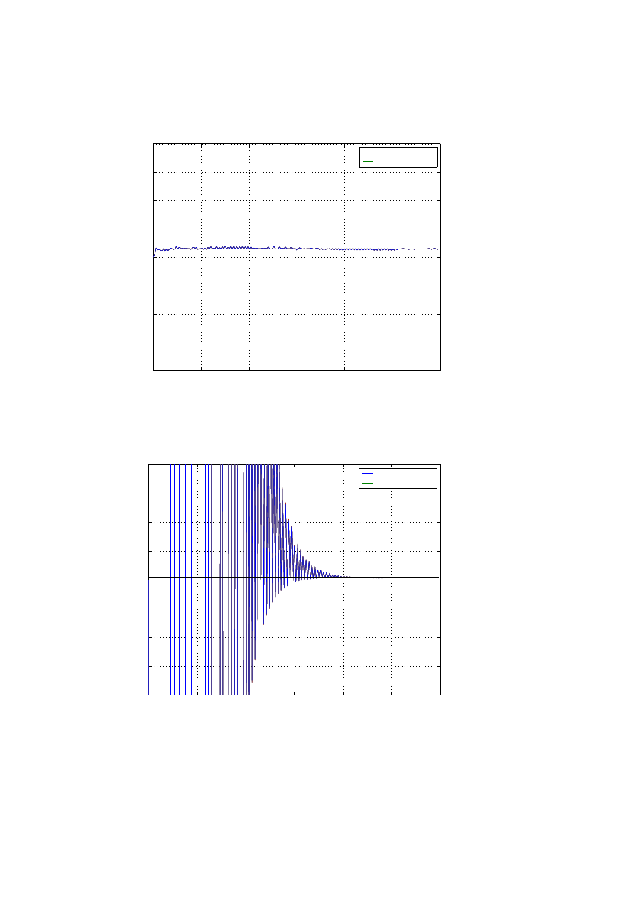
However, α and β differ by an order of N and so it may be improbable that the two
parameters converge to their true value and even if they do, convergence is very slow.
This is reflected from the plots of ˆ
a
t
and ˆb
t
pasted in Fig 5 and Fig 6. Note that the

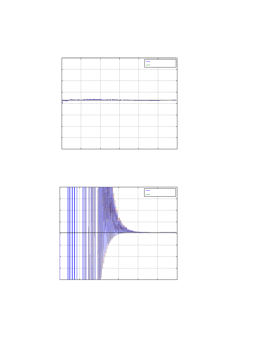
two parameters are related by (10). So, while we can use the LMS update equation
(20) for ˆ
a
t
, ˆb
t
can be estimated as
ˆb
t
=
1 + ˆ
a
t
Z
t−1
−
Z
t
Z
2
t−1
(22)
The results obtained are shown in Figure 7 and Figure 8.
5
Gloabal Estimates
As suggested by the model for malware monitoring (Figure 1), ISPs can share the in-
network estimates to estimate the global trend. As the estimates are computed in a
distributed but coordinated manner, the estimates at various monitors in the network
would be simply delayed copies of each other. So any egress monitor can play the
role of second-tier monitor as well. We consider two approaches in this section - the
first one is simple merging equivalent to flooding every node with every other node’s
estimates while the second approach is a very fast distributed averaging technique that
minimizes the convergence time and thereby communication overhead. Note that, it
takes some time to propagate the estimates and reach a consensus, so the rate at which
the second-tier monitors are updated by the first-tier monitors about the local estimates
is constrained by performance of the averaging algorithm.
5.1
Merging Estimates
If there are L ISPs, they need to share amongst each other
• {α}
i=1:L
at time instants t = ∆
g
, 2∆
g
, 3∆
g
, ... where ∆
g
= r × ∆ is the sampling
interval across the ISPs. Note that ∆ is the in-network sampling interval and r is
the factor that determines the ratio of the in-network and across ISPs sampling
rate.
• {I
t
}
i=1:L
at time instants t = ∆
g
, 2∆
g
, 3∆
g
, ...
• {β}
i=1:L
at time instants t = ∆
g
, 2∆
g
, 3∆
g
, ... (optional)
Now, if we were to apply the discrete time model to the entire internet, the global
observations would be as per
I
t
= (1 + α
g
)I
t−1
− β
g
I
2
t−1
(23)
as opposed to the distributed observations that we have as per
I
t,j
= (1 + α
j
)I
t−1,j
− β
j
I
2
t−1,j
(24)
Now, I
t
=
P
L
j=1
I
t,j
, so that quite intuitively
ˆ
α
g
=
P
L
j=1
α
j
I
t−1,j
P
L
j=1
I
t−1,j
(25)
and,
ˆ
β
g
=
P
L
j=1
β
j
I
2
t−1,j
P
L
j=1
I
2
t−1,j
(26)
The plots for global estimates of α and β (for 2 ISPs) are pasted in Figure 9 and
Figure 10. The estimates for 10 ISPs sharing the scan-data is plotted in Figure 11. As
is expected more data gives better estimate and thus we see a smoothed curve with

lesser error-variance. In a pracical scenario there may be attacks that, due to different
netork topologies, present different infection rates. A similar case was simulated for
gaussian distributed scan-rates (mean = 0.0286, var = 0.0001) across the ISPs and the
global estimate is plotted in Figure 12.
5.2
Fast Distributed Linear Averaging
Fast distributed linear averaging ([3]) techniques may be employed to propagate the
global estimates across ISPs. Given L nodes in a network, the distributed linear itera-
tions have the form
x
i
(t + 1) =
L
X
j=1
W
ij
x
j
(t)
(27)
where weights W
ij
= 0 if {i, j} do not form an edge (i.e. they do not communicate
directly). In vector form the above equation can be written as
x(t + 1) = Wx(t)
(28)
Therefore after t such iterations
x(t + 1) = W
t
x(0)
(29)
and the objective is to choose the weight matrix W such that for any initial value x(0),
x(t) converges to the average vector
¯
x = (11
T
/n)x(0)
(30)
Xiao et. al. ([3]) show that for the convergence the necessary and sufficient conditions
are
• 1 is a left eigenvector of W associated with eigenvalue one. This implies that sum
of the vector of node values is preserved at each step
1
T
x(t + 1) = 1
T
x(t)
(31)
• 1 is also right eigenvector of W associated with eigenvalue one. This implies that
any vector with constant entries is a fixed point of the linear iteration.
W1 = 1
(32)
• One is a simple eigenvalue of W and all other eigenvalues are less than one.
• The Markov chain associated with the iteration is irreducible and aperiodic i.e.
the spectral radius of the matrix (W − 11
T
/n) < 1
5.2.1
Laplacian Techniques
The problem above can be investigated by eigenanalysis of the Laplacian matrix of the
associated graph. Consider a graph comprising of N nodes and M neighbours. The
incidence matrix A ∈ R
N ×M
is defined as
A
mn
=
1
if edge m starts from node n
−1
if edge m ends at node n
0
otherwise
(33)
and the Laplacian matrix of the graph is defined as L = AA
T
. L is positive semidefinite
and as graph is assumed connected L has eigenvector 1 associated with eigenvalue zero.

Figure 2: A network with 8 ISPs
Also, the weights associated with edges are assumed symmetric, so the weight vector
w ∈ R
M
and weight matrix W is
W = I − Adiag(w)A
T
(34)
This form of the matrix W satisfies the conditions in equations (31) and (32) and
reduces the spectral-radius minimization problem to that of spectral norm minimization,
i.e.
minimizekI − Adiag(w)A
T
/nk
2
(35)
Consider 8 ISPs sharing their network estimates with each other. The ISPs commu-
nicate only with their neighbours and the associated graph for the scnario is as shown
in Figure 2. Some of the techniques to reach a fast consensus are discussed below and
the global estimates from the simulations are pasted in Figures 13, 14, 15 and 16.
5.2.2
Best Constant Weight
Simplest approach is to use constant edge weights. Minimizing (33) then gives
w =
2
λ
1
(L) + λ
N −1
(L)
(36)
where λ
i
is the i
th
largest eigenvalue of laplacian matrix.
5.2.3
Maximum Degree Weights
Another simple approach is to have a constant weight for all edges given as the inverse
of maximum number of neighbours any node has in the graph. i.e.
w =
1
d
max
(37)
where d
max
is called the maximum degree of the graph. This approach is quite intuitive
in the sense that the node with maximum neighbours would converge to the average
fastest if it weighs all its neighbours equally.
5.2.4
Local degree weights
This approach is an extension of maximum degree weights. Weight on an edge is given
as inverse of larger of degrees of the incident nodes i.e.
w
m
=
1
max{d
i
, d
j
}
(38)
where edge is made of nodes i and j.

5.2.5
Optimum Symmetric Weights
The optimum symmetric weights are obtained by interior point methods for minimizing
the spectral radius. For more details refer to [3].
6
Results
Pasted below are the estimates of α and β obtained through the MMSE estimator, LMS
filtering as well as those obtained through Towsley’s Kalman filtering (Figure 17). The
simplified MMSE approach assumes the knowledge of total vulnerable population while
the LMS approach and towlsey estimates do not. While with towsley method we can
accurately estimate either α or β, LMS estimates converge both for α and β. Also plot-
ted below are global estimates using various averaging techniques. The simulations are
done for code-red worm propagation and all schemes not only detect the worm activity
but also estimate the infection rate accurately. The estimtes for a non-worm activity
are plotted in Figure 18
7
References
1. Michael Rabbat and Robert Nowak, “Distributed Optimization in Sensor Net-
works” in ISPN, April 2004.
2. C. C. Zou, L. Gao, W. Gong, and D. Towsley, “Monitoring and Early Warning
for Internet Worms”. in 10th ACM Conference on Computer and Communication
Security (CCS03), Oct. 27-31, Washington DC, 2003.
3. Lin Xiao and Stephen Boyd, “Fast Linear Iterations for Distributed Averaging”
to appear in Systems and Control Letters, 2004.
4. CNN technology news http://edition.cnn.com/2003/TECH/internet/01/25/internet.attack/
5. USA-Today “The cost of ‘Code Red’: $1.2 billion” http://www.usatoday.com/tech/news/2001-
08-01-code-red-costs.htm
6. CERT Coordination Center http://www.cert.org
7. Cooperative association for Internet Data Analysis http://www.caida.org
8. SANS Institute http://www.sans.org
0
100
200
300
400
500
600
0
0.5
1
1.5
2
2.5
3
3.5
4
x 10
5
Time t (in minutes)
Number Of Infected hosts
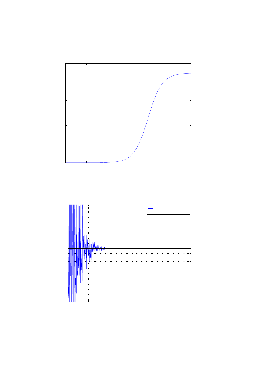
Data collected at monitor 1
Figure 3: Scan-Data Observed at the monitor
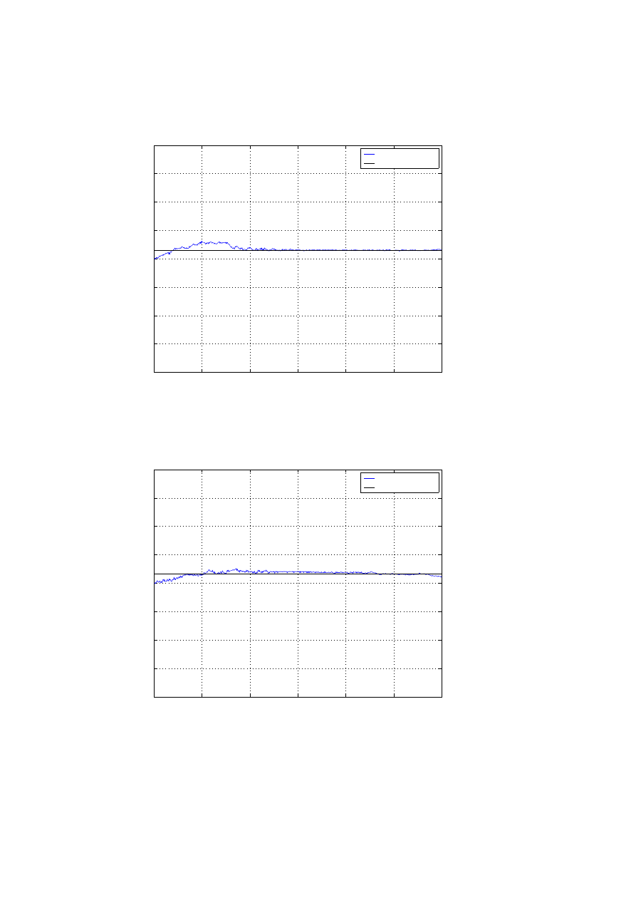
0
100
200
300
400
500
600
−0.25
−0.2
−0.15
−0.1
−0.05
0
0.05
0.1
0.15
0.2
0.25
Time t (in minutes)
Infection Rate
Infection rate estimated at monitor 1
estimated infection rate (
α
~
)
actual rate (
α
)
Figure 4: Our Estimates
0
100
200
300
400
500
600
−0.4
−0.3
−0.2
−0.1
0
0.1
0.2
0.3
0.4
Time t (in minutes)
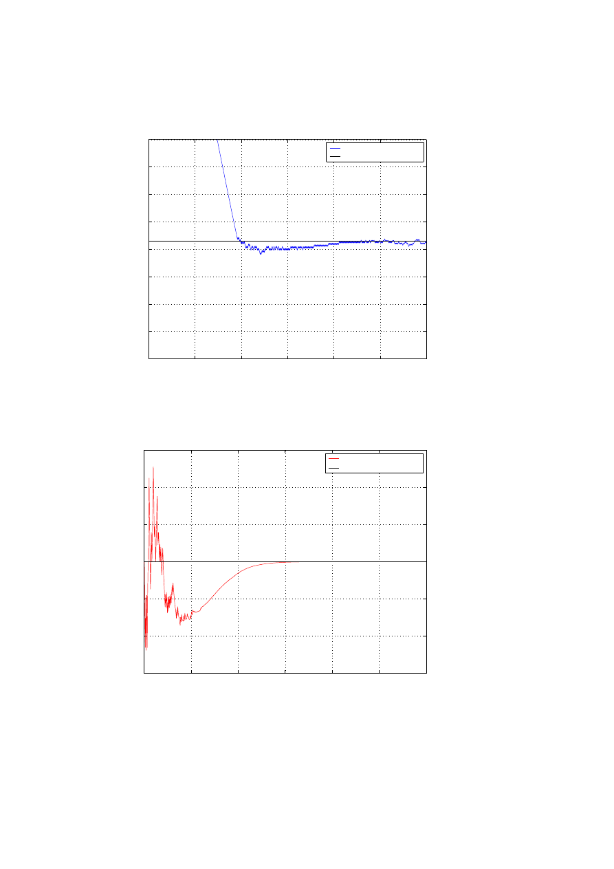
Infection Rate
LMS estimate at monitor 1
estimated infection rate (
α
~
)
actual rate (
α
)
Figure 5: LMS estimate (ˆ
α
)
0
100
200
300
400
500
600
−6
−4
−2
0
2
4
6
x 10
−3
Time t (in minutes)
Infection Rate
LMS estimate at monitor 1
estimated infection rate (
β
~
)
actual rate (
β
)
Figure 6: LMS estimate ( ˆ
β
)
0
100
200
300
400
500
600
−0.4
−0.3
−0.2
−0.1
0
0.1
0.2
0.3
0.4
Time t (in minutes)
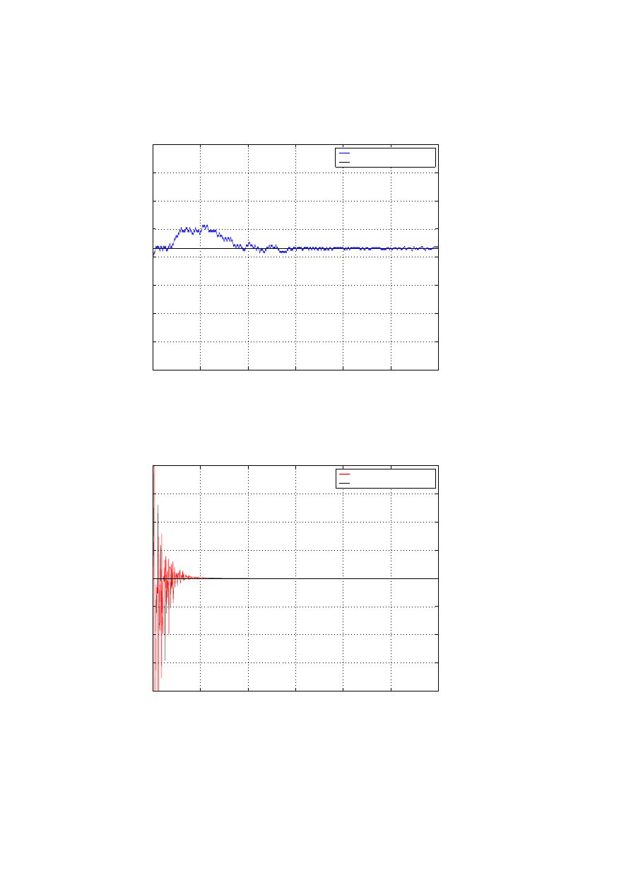
Infection Rate
LMS estimate at monitor 1
estimated infection rate (
α
~
)
actual rate (
α
)
Figure 7: LMS estimate (ˆ
α
)
0
100
200
300
400
500
600
−0.4
−0.3
−0.2
−0.1
0
0.1
0.2
0.3
0.4
Time t (in minutes)
Infection Rate
LMS estimate at monitor 1
estimated infection rate (
β
~
)
actual rate (
β
)
Figure 8: LMS estimate ( ˆ
β
)
0
100
200
300
400
500
600
−0.4
−0.3
−0.2
−0.1
0
0.1
0.2
0.3
0.4
Time t (in minutes)
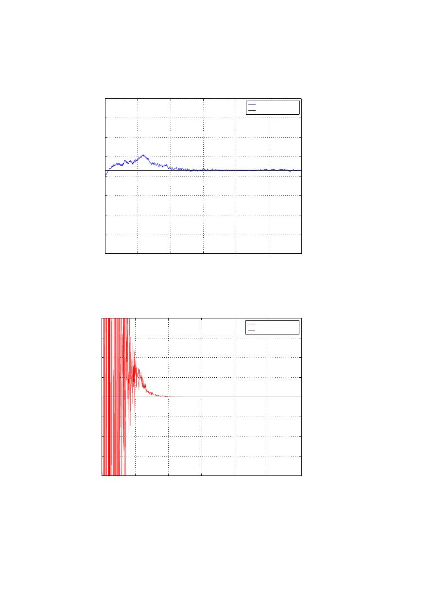
Infection Rate
Global Estimate with 2 ISPs
Global Estimate(
α
~
)
actual rate (
α
)
Figure 9: Global Estimate (α) with 2 ISPs using Estimates merging
0
100
200
300
400
500
600
−4
−3
−2
−1
0
1
2
3
4
x 10
−3
Time t (in minutes)
Infection Rate
Global Estimate with 2 ISPs
Global Estimate(
β
~
)
actual rate (
β
)
Figure 10: Global Estimate (β) with 2 ISPs using Estimates merging
0
100
200
300
400
500
600
−0.4
−0.3
−0.2
−0.1
0
0.1
0.2
0.3
0.4
Time t (in minutes)
Infection Rate
Global Estimate with 10 ISPs
Global Estimate(
α
~
)
actual rate (
α
)
Figure 11: Global Estimate (α) with 10 ISPs using Estimates merging
0
100
200
300
400
500
600
−0.4
−0.3
−0.2
−0.1
0
0.1
0.2
0.3
0.4
Time t (in minutes)
Infection Rate
Global Estimate (Gaussian Distributed
α
) with 10 ISPs
Global Estimate(
α
~
)
actual rate (
α
)
Figure 12: Global Estimate with Gaussian dist. infection rates(α) using Estimates merging
0
100
200
300
400
500
600
−0.4
−0.3
−0.2
−0.1
0
0.1
0.2
0.3
0.4
Time t (in minutes)
Infection Rate
Global Estimate with optimum symmetric weights
Global Estimate(
α
~
)
actual rate (
α
)
Figure 13: Global Estimate of (α) with optimum symmetric weights
0
100
200
300
400
500
600
−4
−3
−2
−1
0
1
2
3
4
x 10
−6
Time t (in minutes)
Infection Rate
Global Estimate with optimum symmetric weights
Global Estimate(
β
~
)
actual rate (
β
)
Figure 14: Global Estimate of (β) with optimum symmetric weights
0
100
200
300
400
500
600
−0.4
−0.3
−0.2
−0.1
0
0.1
0.2
0.3
0.4
Time t (in minutes)
Infection Rate
Global Estimate with best constant weights
Global Estimate(
α
~
)
actual rate (
α
)
Figure 15: Global Estimate of (α) with best constant weights
0
100
200
300
400
500
600
−4
−3
−2
−1
0
1
2
3
4
x 10
−6
Time t (in minutes)
Infection Rate
Global Estimate with best constant weights
Global Estimate(
β
~
)
actual rate (
β
)
Figure 16: Global Estimate of (β) with best constant weights
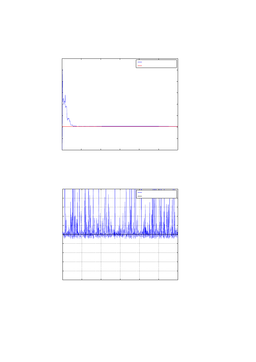
0
100
200
300
400
500
600
−1
−0.5
0
0.5
1
1.5
2
2.5
3
Time t (in minutes)
Infection Rate
TOWSLEY estimate at monitor 1
estimated infection rate (
α
~
)
actual rate (
α
)
Figure 17: Towsley Kalman Filter Estimates
0
100
200
300
400
500
600
−10
−8
−6
−4
−2
0
2
4
6
8
10
Time t (in minutes)
Infection Rate
Non−Worm activity
estimated infection rate (
α
~
)
actual rate (
α
)
Figure 18: Estimates with non-worm activity
Wyszukiwarka
Podobne podstrony:
Detecting Worms through Cryptographic Hashes
Host Based Detection of Worms through Peer to Peer Cooperation
11 centralne monitorowanie poprzez vital sign monitor
09 centralne monitorowanie poprzez center v2
Broadband Network Virus Detection System Based on Bypass Monitor
Countering Network Worms Through Automatic Patch Generation
An Effective Architecture and Algorithm for Detecting Worms with Various Scan Techniques
Detecting Worms via Mining Dynamic Program Execution
Detector De Metales
Notes Centrala Alarmowa SATEL CA-6i, Alarmy i Monitoring
Centrais De Apoio Aos Transportes
Curso De Monitores Lcd(1)
Detector De Metales
Trement F Romanisation et dynamiques territoriales en Gaule centrale Le cas de la cite des Arvernes
CentralAdmin EPLAN 19 de DE
Intrusion Detection for Viruses and Worms
więcej podobnych podstron