Fractional Iteration of Series and Transseries

G. A. Edgar

February 11, 2010

Abstract

We investigate compositional iteration of fractional order for transseries. For any

large positive transseries T of exponentiality 0, there is a family T

[s]

indexed by real

numbers s corresponding to iteration of order s. It is based on Abel’s Equation. We also
investigate the question of whether there is a family T

[s]

all sharing a single support set.

A subset of the transseries of exponentiality 0 is divided into three classes (“shallow”,
“moderate” and “deep”) with different properties related to fractional iteration.

Introduction

Since at least as long ago as 1860 (A. Cayley [3]) there has been discussion of real
iteration groups (compositional iteration of fractional order) for power series. Or at
least for formal power series, where we do not worry about convergence of the result.
In this paper we adapt this to transseries. In many cases it is, in fact, not difficult
to do when we ignore questions of convergence.

We will primarily use the ordered differential field T = R G

= R x

of (real

grid-based) transseries; T is also known as the transline. So T is the set of all grid-
based real formal linear combinations of monomials from G, while G is the set of all
e

for L ∈ T purely large. (Because of logarithms, there is no need to write separately

two factors as x

.) See “Review” below.

The problem looks like this: Let T be a large positive transseries. Is there a

family T

[s]

of transseries, indexed by reals s, so that: T

[0]

(x) = x, T

[1]

= T , and

[s]

◦ T

[t]

= T

[s+t]

for all s, t ∈ R? These would be called fractional iterates of T :

U = T

[1/2]

satisfies U ◦ U = T ; or T

[−1]

is the compositional inverse of T ; etc. We limit

this discussion to large positive transseries since that is where compositions S ◦ T are
always defined. In Corollary 4.5 we conclude (in the well-based case) that any large
positive T of exponentiality 0 admits such a family of fractional iterates. However,
there are grid-based large positive transseries T and reals s for which the fractional
iterate T

[s]

is not grid-based (Example 4.8).

We also investigate the existence of a family T

[s]

, s ∈ R, all supported by a single

grid (in the grid-based case) or by a single well-ordered set (in the well-based case).
We show that such a family exists in certain cases (Theorems 3.7 and 3.8) but not in
other cases (Theorem 3.9).

Review

The differential field T of transseries is completely explained in my recent expository
introduction [9]. Other sources for the definitions are: [1], [5], [8], [15]. I will generally
follow the notation from [9]. The well-based version of the construction is described in
[8] (or [10, Def. 2.1]). In this paper it is intended that all results hold for both versions,
unless otherwise noted. (I use labels G or W for statements or proofs valid only for
the grid-based or well-based version, respectively.) We will write T, G, and so on in
both versions.

Write P = { S ∈ T : S ≻ 1, S > 0 } for the set of large positive transseries. The

operation of composition T ◦ S is defined for T ∈ T, S ∈ P. The set P is a group under
composition ([15, § 5.4.1], [8, Cor. 6.25], [10, Prop. 4.20], [11, Sec. 8]). Both notations
T ◦ S and T (S) will be used.

We write G for the ordered abelian group of transmonomials. We write G

N,M

for

the transmonomials with exponential height N and logarithmic depth M . We write
G

for the log-free transmonomials with height N . Even in the well-based case, the

definition is restricted so that for any T ∈ T there exists N, M with supp T ⊆ G

N,M

The support supp T is well ordered for the converse of the relation ≺ in the well-
based case; the support supp T is a subgrid in the grid-based case. A ratio set µ is
a finite subset of G

small

; J

is the group generated by µ. If µ = {µ

, · · · , µ

}, then

: k ∈ Z

. If m ∈ Z

, then J

: k ∈ Z

, k ≥ m

is a grid. A

grid-based transseries is supported by some grid. A subgrid is a subset of a grid.

For transseries A, we already use exponents A

for multiplicative powers, and paren-

theses A

(n)

for derivatives. Therefore let us use square brackets A

[n]

for compositional

powers. In particular, we will write A

[−1]

for the compositional inverse. Thus, for

example, exp

= exp

[n]

= log

[−n]

In this paper we will be using some of the results on composition of transseries from

[10] and [11], where the proofs are sometimes not as simple as in [9] (and not all of
them are proved there).

Motivation for Fractional Iteration

Before we turn to transseries, let us consider fractional iteration in general. Given
functions T : X → X and Φ: R × X → X, we say that Φ is a real iteration group
for T iff

Φ(s + t, x) = Φ s, Φ(t, x)

(1)

Φ(0, x) = x,

(2)

Φ(1, x) = T (x),

(3)

for all s, t ∈ R and x ∈ X.

Let us assume, say, that X is an interval (a, b) ⊆ R, possibly a = −∞ and/or

b = ∞, and that Φ has as many derivatives as needed. If we start with (1), take the
partial derivative with respect to t,

(s + t, x) = Φ

s, Φ(t, x)

(t, x),

then substitute t = 0, we get

(s, x) = Φ

(s, x) Φ

(0, x).

(4)

We have written Φ

and Φ

for the two partial derivatives of Φ. Equation (4) is the

one we will be using in Sections 2 and 3 below. Here is a proof showing how it works
in the case of functions on an interval X.

Proposition 1.1.

Suppose Φ : R × X → X satisfies (2) and

(s, x) = Φ

(s, x) β(x)

′

)

with β(x) > 0. [Assume also ∞ =

dy/β(y) and ∞ =

dy/β(y) for x

∈ X =

(a, b).] Then Φ satisfies (1) with β(x) = Φ

(0, x).

Proof. Fix x

∈ X. Let θ(t) be the solution of the ODE θ

′

(t) = β(θ(t)), θ(0) = x

That is, θ(t) = x is defined implicitly by

β(y)

= t.

[In order to get all time t, we need ∞ =

dy/β(y) and ∞ =

dy/β(y).] Consider

F (u, v) = Φ(u + v, θ(u − v)). Then

(u, v) = Φ

u + v, θ(u − v)

− Φ

u + v, θ(u − v)

′

(u − v)

= Φ

u + v, θ(u − v)

− Φ

u + v, θ(u − v)

β θ(u − v)

= 0

by (4

′

). This means F is independent of v. So

θ(t) = Φ(0, θ(t)) = F (t/2, −t/2) = F (t/2, t/2)

= Φ(t, θ(0)) = Φ(t, x

Φ(s, Φ(t, x

)) = Φ(s, θ(t)) = F ((s + t)/2, (s − t)/2)

= F ((s + t)/2, (s + t)/2) = Φ(s + t, θ(0)) = Φ(s + t, x

Differentiate Φ(t, x

) = θ(t) to get Φ

(t, x

) = θ

′

(t) = β(θ(t)), then substitute t = 0 to

get Φ

(0, x

) = β(θ(0)) = β(x

Three Examples

Power Series

We start with the classical case of power series. (A. Cayley 1860 [3]; A. Korkine 1882
[17].) We will think of formal power series (for x → ∞), and not actual functions.
Consider a series of the form

T (x) = x



1 +

∞

j=1

−j





(5)

= x +

∞

j=1

−j+1

= x + c

+ c

−1

+ c

−2

+ · · ·

Such a series admits an iteration group of the same form. That is,

Φ(s, x) = x



1 +

∞

j=1

(s)x

−j



 .

(6)

In fact, α

(s) is sc

+ {polynomial in s, c

, c

, . . . , c

j−1

with rational coefficients, of

degree j − 1 in s}. The first few terms:

Φ(s, x) = x + sc

+ sc

−1

s(1 − s)

−2

s(1 − s)

(2c

+ c

) +

s(1 − s)(1 − 2s)

−3

+ · · · .

Theorem 2.1.

Let T (x) be the power series (5). Define α

: R → R recursively by

(s) = sc

(s) = s



c

−

(−j

+ 1)α

(u)α

′

(0) du





(−j

+ 1)α

(u)α

′

(0) du.

Then the series Φ defined formally by (6) is a real iteration group for T .

Proof. Check (2), (3), (4).

Remark 2.2. The formulas are obtained by plugging (6) into (4), equating coefficients,
then integrating the resulting ODEs. Consequently, this is the unique solution of the
form (6) with differentiable coefficients.
Remark 2.3. Of course there is a corresponding formulation for series of the form

T (z) = z



1 +

∞

j=1



 = z + c

+ c

+ · · · .

Then we get Φ(s, z) = z 1 +

∞

j=1

(s)z

, with

(s) = sc

(s) = s



c

−

+ 1)α

(u)α

′

(0) du





+ 1)α

(u)α

′

(0) du.

The first few terms are:

Φ(s, z) = z + sc

+ sc

+ s(s − 1)c

5s(s − 1)

s(s − 1)(2s − 3)

+ · · · .

Convergence

We considered here formal series. Even if (5) converges for all x (except 0), it need
not follow that (6) converges. Indeed, one of the criticisms of Cayley [3] and Korkine
[17] was that convergence was not proved. Baker [2] provides examples where a power
series converges, but none of its non-integer iterates converges. Erd¨os & Jabotinsky
[13] investigate the set of s for which the series converges.

Transseries, Height and Depth 0

Let B ⊆ (0, ∞) be a well ordered set (under the usual order). The transseries

T (x) = x

1 +

b∈B

−b

= x +

b∈B

−b+1

(7)

is the next one we consider. In fact, the additive semigroup generated by B is again
well ordered (Higman, see the proof in [10, Prop. 2.2]), so we will assume from the start
that B is a semigroup. If B is finitely generated, then (7) is a grid-based transseries.
But in general it is well-based. If B is finitely generated, then B has order type ω. But
of course a well ordered B can have arbitrarily large countable ordinal as order type.

We claim T has a real iteration group supported by the same 1 − B, where B is a

well-ordered additive semigroup of positive reals.

Proposition 2.4.

Let B ⊆ (0, ∞) be a semigroup. The transseries (7) has a real

iteration group

Φ(s, x) = x

1 +

b∈B

(s)x

−b

Proof. The only thing needed is that B is a well ordered semigroup. It follows that,
for any given b ∈ B, there are just finitely many pairs (b

, b

) ∈ B × B with b

+ b

= b

[9, Prop. 3.27]. Then define recursively:

(s) =

(−b

+ 1)α

(s)α

′

(0),

(s) = s

−

(u) du

(u) du.

For each b, both f

(s) and α

(s) are polynomials (finitely many terms!) in s and the

[with b

< b except for the term sc

]. Check (2), (3), (4).

A Moderate Example

Now we consider another case. We single it out because it occurs frequently enough to
make it useful to have the formulas displayed. Consider the transseries

T (x) = x





∞

k=0

∞

j=0

j,k

−j

−kx



 ,

0,0

= 1.

(8)

The set

B = { (j, k) : k ≥ 0, j ≥ 0, (j, k) 6= (0, 0) }

(9)

is a semigroup under addition. The set

−j

−kx

: (j, k) ∈ B

is then a semigroup

under multiplication. It is well ordered with order type ω

with respect to the converse

of ≻.

Theorem 2.5.

Let B be as in (9). Then the transseries (8) admits a real iteration

group supported by the same set

1−j

−kx

: j, k ≥ 0

Proof. Write

Φ(s, x) = x



1 +

(j,k)∈B

j,k

(s)x

−j

−kx



 .

(A) We first consider the case with c

1,0

= 0. The coefficient functions α

j,k

are

defined recursively as follows. If (j, k) /

∈ B, then let α

j,k

(s) = 0. Let (j, k) ∈ B and

assume α

(s) have already been defined for all (j

, k

) with either k

< k or {k

= k

and j

< j}. Then let

j,k

(s) =

(−j

+ 1)α

′

(0) − k

′

+1,k

(0)

(s),

where the sum is over all j

, j

, k

with j

+ j

= j, k

+ k

= k. Check that all

the terms in the sum involve α’s that have already been defined (or are multiplied by
zero); this depends on c

1,0

= 0, so α

1,0

(s) = 0. Define F

j,k

(s) =

j,k

(u) du and

j,k

(s) = c

j,k

− F

j,k

(1)

s + F

j,k

(s).

Check (2), (3), (4).

(B) Now consider the case with c

1,0

6= 0. Write c = c

1,0

. The coefficient functions

j,k

are defined recursively as follows. If (j, k) /

∈ B, then let α

j,k

(s) = 0. Let (j, k) ∈ B

and assume α

(s) have already been defined for all (j

, k

) with either k

< k or

= k and j

< j}. Then let

j,k

(s) =

(−j

+ 1)α

′

(0) − k

′

+1,k

(0)

(s),

where the sum is over all j

, j

, k

with j

+ j

= j, k

+ k

= k. Omit the terms

′

(0) and −kcα

(s) and terms with a factor 0. Then all terms in the sum involve

α’s already defined. Define F

j,k

(s) =

kc(u−s)

j,k

(u) du and

j,k

(s) =











j,0

− F

j,0

(1)

s + F

j,0

(s),

if k = 0,

j,k

− F

j,k

(1)

1 − e

−sck

1 − e

−ck

+ F

j,k

(s),

if k > 0.

Recall c = c

1,0

. Check (2), (3), (4).

In case (B)—the “moderate case”—the coefficients α

j,k

(s) are not necessarily poly-

nomials in s.

A Deep Example

Another simple example shows that real iteration group of that type need not always
exist. Let B ⊆ Z

B = { (j, 0, 0) : j ≥ 1 } ∪ { (j, k, 0) : k ≥ 1 } ∪ { (j, k, l) : l ≥ 1 } .

(10)

Then

−j

−kx

−lx

: (j, k, l) ∈ B

is a semigroup, but not well ordered.

I included some negative j and k so that the set of transseries of the form



1 +

(j,k,l)∈B

jkl

−j

−kx

−lx





(where of course each individual support is well ordered, not all of B) is closed under
composition.

Proposition 2.6.

Let B

′

be a well ordered subset of (10). The transseries T (x) =

x(1 + x

−1

+ e

−x

) admits no real iteration group of the form

Φ(s, x) = x



1 +

(j,k,l)∈B

′

jkl

(s)x

−j

−kx

−lx



 .

Proof. We may assume B

′

= { (j, k, l) : α

jkl

6= 0 }. As before, the first term beyond x

can be computed as α

100

(s) = s · 1 = s, so α

′

100

(s) = 1. Now α

001

(1) 6= 0, so there

is a least (j, k, 1) ∈ B

′

. But then by considering the coefficient of x

2−j

−kx

−x

(s, x) = Φ

(s, x)Φ

(0, x) we have

0 = (−2)α

jk1

(s)α

′

100

(0),

so α

jk1

(s) = 0, a contradiction.

Remark 2.7. An alternate argument that there is no grid (or well ordered set) support-
ing a real iteration group for T = x + 1 + xe

−x

. Compute

supp T

[−1]

= {x ≻ 1 ≻ xe

−x

≻ · · · }

supp T

[−2]

= {x ≻ 1 ≻ xe

−x

≻ · · · }

supp T

[−3]

= {x ≻ 1 ≻ xe

−x

≻ · · · }

. . .

supp T

[−k]

= {x ≻ 1 ≻ xe

2kx

−x

≻ · · · },

k ∈ N, k > 0.

So there is no grid (and no well ordered set) containing all of these supports.

The Case of Common Support

Conjugation

The set P of large positive transseries is a group under composition ([10, Prop. 4.20], [11,
Sec. 8]). In a group, we say U, V are conjugate if there exists S with S

[−1]

◦U ◦S = V .

Then for all k ∈ N it follows that S

[−1]

◦ U

[k]

◦ S = V

[k]

. If Φ(s, x) is an iteration group

for U (x), then S

[−1]

(Φ(s, S(x))) is an iteration group for the conjugate S

[−1]

(U (S(x))).

This can be used to reduce the question of fractional iteration for certain more general
transseries to more restricted cases to be discussed here.

Puiseux series

For a Puiseux series of the form

T =

∞

j=m

−j/k

(11)

(m ∈ Z, k ∈ N, c

> 0), we can conjugate with x

1/k

◦ T ◦ x

T (x

)

1/k





∞

j=m

−j





1/k

= c

1/k

−m/k

1 + c

m+1

−1

+ c

m+2

−2

+ · · ·

1/k

= c

1/k

−m/k

1 + a

−1

+ a

−2

+ · · ·

If dom T = x, then also dom(x

1/k

◦ T ◦ x

) = x and existence of a real iteration group

is then clear from Proposition 5. (If dom T 6= x, keep reading.)

Exponentiality

Associated to a general T ∈ P is an integer p called the exponentiality of T [15,
Ex. 4.10] [10, Prop. 4.5] such that for all large enough k ∈ N we have log

◦ T ◦ exp

∼

exp

. Write p = expo T .

Now expo(S ◦ T ) = expo S + expo T , so no transseries with nonzero exponentiality

can have a real iteration group of transseries. There is no transseries T with T ◦T = e

(But see [12].) The main question will be for exponentiality zero. If expo T = 0, then
T is conjugate to some S = log

◦ T ◦ exp

such that S ∼ x and such that S is log-free

[10, Prop. 4.8]. So we will deal with this case.

Shallow—Moderate—Deep

Now we turn to the general large positive log-free transseries with dominant term x.
It admits a unique real iteration group with a common support in many cases (shallow
and moderate), but not in many other cases (deep).

Definition 3.1. Consider log-free T ∼ x. A real iteration group for T with common
support

is a real iteration group Φ(s, x) of the form

Φ(s, x) = x



1 +

∈B

(s)g





(12)

for some subgrid ( W or well ordered) B

⊆ G (not depending on s) where coefficient

functions α

: R → R are differentiable.

Write T = x(1 + U ), U ≺ 1, U ∼ ae, a ∈ R, a 6= 0, e ∈ G, e ≺ 1. As before, if there

is a real interation group Φ, it begins Φ(s, x) = x(1 + sae + · · · ). We may assume: if
g

∈ B, then α

(s) 6= 0 for some s. So the greatest element of B is e.

Write A

†

= A

′

/A for the logarithmic derivative.

Definition 3.2. Let T = x(1 + U ), U ≺ 1, mag U = e. Monomial e is called the first
ratio

of T . We say that T is:

shallow

iff g

†

≺ 1/(xe) for all g ∈ supp U;

moderate

iff g

†

1/(xe) for all g ∈ supp U and g

†

≍ 1/(xe) for at least one

∈ supp U;

deep

iff g

†

≻ 1/(xe) for some g ∈ supp U.

purely deep

iff g

†

≻ 1/(xe) for all g ∈ supp U except e.

Remark 3.3. G It may be practical to check these definitions using a ratio set µ =
{µ

, · · · , µ

}. For example: Suppose supp U ⊆ J

. By the group property (Lemma

3.14): if µ

†

≺ 1/(xe) for 1 ≤ i ≤ n, then T is shallow. This will be “if and only if”

provided µ is chosen from the group generated by supp U , which can always be done.

Remark 3.4. The case of two terms, T = x(1 + ae) exactly, is shallow. Indeed, e ≺ 1
and so xe ≺ x, xe

′

≺ 1 and e

′

/e ≺ 1/(xe).

Remark 3.5. For small monomials, the logarithmic derivative operation reverses the
order: if 1 ≻ a ≻ b, then a

†

(Lemma 3.11(e)). And for U ≺ 1 we have U

†

∼

(mag U )

†

(Lemma 3.11(c)). So T = x(1 + ae + V ), V ≺ e, is purely deep if and only if

†

≻ 1/(xe).

Remark 3.6. The condition g

†

≺ 1/(xe) says that g is “not too small” in relation to e.

(This is the reason for the terms “shallow” and “deep”.) If g ≺ 1 then g = e

−L

with

L > 0 purely large and

†

≺

⇐⇒ L

′

≺

⇐⇒ L ≺

⇐⇒ L < c

for all real c > 0

⇐⇒ e

< exp

for all real c > 0

⇐⇒ g > exp

−c

for all real c > 0.

So the set A =

∈ G : g 4 e, g

†

≺ 1/(xe)

is an interval in G. The large end of the

interval is the first ratio e, the small end of the interval is the gap in G just above all
the values exp(−c

(1/xe)), c ∈ R, c > 0. If we write exp −0

(1/xe)

for that gap,

then

exp −0

(1/xe)

, e

I will call this the shallow interval below e. Van der Hoeven devotes a chapter [15,
Chap. 9] to gaps (cuts) in the transline. In his classification [15, Prop. 9.15],

exp −0

(1/xe)

= e−e

A − e

where mag

(1/(xe)) = e

Similarly, the set A =

∈ G : g 4 e, g

†

1/(xe)

is an interval in G. The large

end of the interval is the first ratio e, the small end of the interval is the gap in G just

below all the values exp −c

(1/xe)

, c ∈ R, c > 0. If we write exp −∞

(1/xe)

for

that gap, then

exp −∞

(1/xe)

, e

I will call this the moderate interval below e. In van der Hoeven’s classification,

exp −∞

(1/xe)

= e−e

A + e

where mag

(1/(xe)) = e

The Examples

Let us examine where the examples done above fit in the shallow/deep classification.
If e = x

−1

, then 1/(xe) = 1,

(1/(xe)) = x, exp −c

(1/(xe))

= e

−cx

. The small end

of the shallow interval is exp(−0x). In a power series, every monomial x

−j

≻ e

−0x

inside the shallow interval, so a power series is shallow.

In example (8), we saw two cases. In case c

1,0

6= 0, then e = x

−1

so again the small

end of the shallow interval is exp(−0x). But the monomial x

−j

−kx

≺ exp(−0x) if

k > 0, and is thus outside the shallow interval, so this is not shallow. The small end
of the moderate interval is exp(−∞x), and all monomials x

−j

−kx

≻ exp(−∞x) are

inside the moderate interval, so this is the moderate case.

The other case is c

1,0

= 0. Then e is x

−2

(or smaller). If e = x

−2

, then 1/(xe) = x,

exp −c

(1/(xe))

= e

−(c/2)x

. The small end of the shallow interval is exp(−0x

). All

monomials x

−j

−kx

≻ exp(−0x

) are inside the shallow interval, so this is the shallow

case.

Finally consider the example T = x(1 + x

−1

+ e

−x

) of Proposition 2.6. Since

= x

−1

, the small end of the moderate interval was computed as exp(−∞x). The

monomial e

−x

≺ exp(−∞x) is outside of that, so T is deep.

Proofs

Proofs will follow the examples done above. These proofs use some technical lemmas
on logarithmic derivatives, grids, and well ordered sets; they are found after the main
results, starting with Lemma 3.11.

Theorem 3.7.

If (log-free) T ∼ x is shallow, then T admits a real iteration group with

common support where all coefficient functions are polynomials.

Proof. The proof is as in Proposition 2.4 above. Here are the details. Write T =
x(1 + U ), U ∼ ae, e ≺ 1. Begin with the subgrid ( W well ordered) supp U which is
contained in

∈ G : g < e, g

†

≺ 1/(xe)

. Let B ⊇ supp U be the least set such that

if g

, g

∈ B, then supp (xg

)

′

⊆ B. By Lemma 3.22, B is a subgrid ( W by

Lemma 3.23, B is well ordered) and B ⊆

∈ G : g < e, g

†

≺ 1/(xe)

Write

T (x) = x



1 +

∈B





Φ(s, x) = x



1 +

∈B

(s)g





(s, x) = x

∈B

′

(s)g

(13)

(0, x) = x

∈B

′

(0)g

(s, x) = 1 +

∈B

(s) (xg)

′

(s, x)Φ

(0, x) = x

∈B

′

(0)g + x

∈B

(s)α

′

(0) (xg

)

′

Now fix a monomial g ∈ B. Assume α

has been defined for all g

≻ g. Consider-

ation of the coefficient of xg in (4) gives us an equation

′

(s) = α

′

(0) + f

(s),

(14)

where f

(s) is a (real) linear combination of terms α

(s)α

′

(0) where g

, g

∈ B satisfy

∈ supp (xg

)

′

. By Lemma 3.19 ( W Lemma 3.20), for a given value of g, there

are only finitely many pairs g

, g

involved.

Now I claim these all have g

≻ g and g

≻ g. Indeed, since g ∈ supp (xg

)

′

and (xg

)

′

= g

+ xg

′

, we have either g 4 g

or g 4 xg

′

. Take two cases:

(a) g 4 g

: Now g

, so g 4 eg

≺ g

. And g

, so g 4 eg

≺ g

(b) g 4 xg

′

: Now g

′

≺ g

/(xe) so g 4 xg

′

≺ g

/e. But g

, so g ≺ g

. And

, so g ≺ g

Thus we may use equations (14) to recursively define α

(s). Indeed, solving the differ-

ential equation, we get α

(s) =

(u) du + sα

′

(0) + C; but α

(0) = 0 and α

(1) = c

(s) = s

−

(u) du

(u) du.

(15)

In particular, the recursion begins with g = e where f

(s) = 0 and α

(s) = sc

= sa.

Also (by induction) α

(s) and f

(s) are polynomials in s.

Theorem 3.8.

If (log-free) T ∼ x is moderate, then T admits a real iteration group

with common support. The coefficient functions are entire; we cannot conclude the
coefficient functions are polynomials.

Proof. The proof is as in Theorem 2.5 above. Here are the details. Write T = x(1+U ),
U ∼ ae, e ≺ 1. Begin with the subgrid ( W well ordered) supp U which is contained in

∈ G : g < e, g

†

1/(xe)

. Let B ⊇ supp U be the least set such that if g

, g

∈ B,

then supp (xg

)

′

⊆ B. By Lemma 3.22, B is a subgrid ( W by Lemma 3.23, B is

well ordered) and B ⊆

∈ G : g < e, g

†

1/(xe)

Write T (x) = x(1 +

∈B

) and Φ(s, x) = x(1 +

∈B

(s)g). Compute the

derivatives as in (13).

Now fix a monomial g ∈ B. Assume α

has been defined for all g

≻ g. There are

two cases. If g

†

≺ 1/(xe), then the argument proceeds as before, and we get (15). Now

assume g

†

≍ 1/(xe), say g

†

∼ b/(xe), b ∈ R, b 6= 0. Consideration of the coefficient of

xg in (4) gives us an equation

′

(s) = α

′

(0) + f

(s) + bα

(s)α

′

(0),

(16)

where f

(s) is a (real) linear combination of terms α

(s)α

′

(0) where g

, g

∈ B satisfy

∈ supp (xg

)

′

. The term with g

= g, g

= e, namely bα

(s)α

′

(0), is not included

in f

but written separately. By Lemma 3.19 ( W Lemma 3.20), for a given value of

, there are only finitely many pairs g

, g

involved.

But I claim these all have g

≻ g and g

≻ g except for the case g

= g, g

= e.

Indeed, since g ∈ supp (xg

)

′

and (xg

)

′

= g

+ xg

′

, we have either g 4 g

g 4

′

. Take two cases:

(a) g 4 g

: Now g

, so g 4 eg

≺ g

. And g

, so g 4 eg

≺ g

(b) g 4 xg

′

: Now g

′

/(xe) so g 4 xg

′

/e, with ≍ only if g ≍ xg

′

and g

†

= 1/(xe). But g

, so g 4 g

, and ≍ would mean g

= e and g

†

= 1/(xe)

so e

†

≍ 1/(xe), which is false; thus g ≺ g

. And g

, so g 4 g

. This time ≍

means g

= e, g

= g, g

†

≍ 1/(xe).

Thus we may use equations (16) to recursively define α

(s). Indeed, solving the differ-

ential equation, we get

(s) =

abs

− 1

−

ab(1−u)

(u) du

ab(s−u)

(u) du

(17)

if g

†

∼ b/(xe).

Theorem 3.9.

If (log-free) T ∼ x is deep, then it does not admit a real iteration group

of the form (12).

Proof. The proof is as in Proposition 2.6 above. Here are the details. Write T =
x(1 + U ), U ∼ ae, e ≺ 1. Suppose

Φ(s, x) = x



1 +

∈B

(s)g





satisfies (4), (2), Φ(1, x) = T (x), and B is a subgrid ( W well ordered). We may
assume α

6= 0 for all g ∈ B. Write

∈ B : g

†

1/(xe)

∈ B : g

†

≻ 1/(xe)

(the moderate and deep portions of B). As before, max B = e and α

(s) = as,

′

(0) = a, a 6= 0.

Let m = max B

. So m

†

≻ 1/(xe). Write m

†

∼ −bp/(xe), b ∈ R, b > 0, p ∈ G,

≻ 1. (m is small and positive, so m

′

is negative.) In (4) we will consider the coefficient

of xpm = x mag (xm)

′

. By Lemma 3.11(g), ((xm)

′

)

†

∼ m

†

≻ 1/(xe); by Remark 3.4,

†

≺ 1/(xe); so (pm)

†

= ((xm)

′

)

†

+ e

†

∼ ((xm)

′

)

†

≻ 1/(xe) and pm /

∈ B

. Also pm ≻ m,

so pm /

∈ B

. Thus pm /

∈ B so α

= 0.

I claim the only g

, g

∈ B with pm ∈ supp (xg

)

′

are g

= m, g

= e. To prove

this, consider these cases:

(a) g

≻ m, g

≻ m. By Lemma 3.14(b), supp((xg

)

′

) ⊆ B

and by Lemma 3.14(a),

supp((xg

)

′

) ⊆ B

. So pm /

∈ supp((xg

)

′

(b) g

= m, g

= e. In this case pm = mag((xg

)

′

), so pm ∈ supp((xg

)

′

= m, g

≺ e. Then (xg

)

′

≺ (xm)

′

≍ pm, so pm /

∈ supp((xg

)

′

(d) g

≺ m. Then (xg

)

′

≺ (xm)

′

≍ pm, so pm /

∈ supp((xg

)

′

(e) g

. Then by Remark 3.4, (xg

)

′

(xe)

′

≺ m ≺ pm, so pm /

∈ supp((xg

)

′

So consideration of the coefficient of xpm in (4) yields:

0 = −bα

(s)α

′

(0) = −abα

(s),

where −ab 6= 0, so α

= 0, a contradiction.

Remark 3.10. If T ∼ x, then a calculation shows that T is shallow, moderate, or deep
if and only if log ◦ T ◦ exp is shallow, moderate, or deep, respectively. This invariance
of the classification will show that the three theorems above are correct for all T ∈ T
with T ∼ x, even if not log-free. For example, T = x + log x is shallow, since log-free

log ◦ T ◦ exp = x +

∞

j=1

(−1)

j+1

−jx

is shallow.

Recall that if T is large and positive and has exponentiality 0, then for some k

we have log

[k]

◦ T ◦ exp

[k]

∼ x. We might try to use the same principle to extend the

definitions of shallow, moderate, and deep to such transseries T even if T 6∼ x. Define
T shallow provided log

[k]

◦ T ◦ exp

[k]

is shallow for some k; similarly for moderate and

deep. Examples: T = x log x is shallow, since log ◦ T ◦ exp = x + log x is shallow. The
finite power series U = 2x − 2/x is moderate, since

log ◦ U ◦ exp = x + log 2 −

∞

j=1

−2jx

is moderate. And V = 2x − 2e

−x

is deep.

But the usefulness of this extension is not entirely clear, since it may produce

a family Φ(s, x) without common support. Example: For T = x log x we compute
S = log ◦ T ◦ exp = x + log x. So we get a real iteration group for S of the form
Ψ(s, x) = x + s log x + o(1), and then a real iteration group for T of the form Φ(s, x) =
exp(Ψ(s, log x)) = x(log x)

+ · · · . These are not all supported by a common subgrid

or even a common well ordered set. When the support depends on the parameter s, it
may no longer make sense to require the coefficients be differentiable.

Example x

+ c is also deep. It is discussed in Section 6, below. The figure there

illustrates supports of iterates M

[s]

that vary with s.

Technical Lemmas

Lemma 3.11.

Let a, b ∈ G and A, B ∈ T. (a) If a = e

, with A 6= 0 purely large, then

†

= A

′

. (b) (AB)

†

= A

†

+ B

†

. (c) If A = ag(1 + U ), g 6= 1, U ≺ 1, then A

†

∼ g

†

(d) If 1 ≺ a 4 b, then a

†

. (d

′

) If 1 ≺ A 4 B, then A

†

. (e) If 1 ≻ a < b,

then a

†

. (e

′

) If 1 ≻ A < B, then A

†

. (f) If b ≺ a ≺ 1/b, then a

†

. (g) If

6= 1 is log-free and n ∈ supp (xb)

′

, then n

†

∼ b

†

Proof. (a) a

′

= A

′

so a

†

= a

′

/a = A

′

(b) Product rule.
(c) Since g = e

, L purely large, note g

†

= L

′

. Also U ≺ 1 so (1+U)

†

= U

′

/(1+U ) ∼

′

. Now L ≻ 1 ≻ U, so L

′

≻ U

′

and g

†

≻ (1 + U)

†

. So A

†

= a

†

+ g

†

+ (1 + U )

†

∼ g

†

(d) Write a = e

, b = e

, with A, B purely large. Now 0 < A ≤ B, so A 4 B. Also

B 6≍ 1, so A

′

, that is, a

†

. (d

′

) follows from (c).

(e) Write a = e

, b = e

, with A, B purely large. Now 0 > A ≥ B, so A 4 B. Also

B 6≍ 1, so A

′

, that is, a

†

. (e

′

) follows from (c).

(f) If a = 1, then a

†

= 0. If a ≺ 1, then apply (e). If a ≻ 1, note that b

†

−(1/b)

†

≍ (1/b)

†

, then apply (d).

(g) Case 1: b = x

, b ∈ R, b 6= 0. Then xb = x

b+1

, (xb)

′

= (b + 1)x

∼ b. So

((xb)

′

)

†

∼ b

†

. Case 2: b = x

, L 6= 0 has height n ≥ 0. Assume b ≺ 1, the case b ≻ 1

is similar. Then xb = x

b+1

, (xb)

′

= ((b + 1) + xL

′

= Ab where A = (b + 1) + xL

′

has height n. Now n ∈ supp (xb)

′

, so n = ab where a ∈ supp A. But a has height n,

so by “height wins” [9, Prop. 3.72], we have b ≺ a ≺ 1/b. In the proofs of (d) and (e),
if it is a case of “height wins” then we get strict inequality A ≺ B and a

†

≺ b

†

. So

here a

†

≺ b

†

. Therefore n

†

= (ab)

†

= a

†

+ b

†

∼ b

†

Lemma 3.12.

Let T = x(1 + ae + o(e)) with e ∈ G, e ≺ 1, a ∈ R, a > 0. Let g ∈ G,

≺ 1. Then (i) e(T ) ∼ e; (ii) if g ≺ 1/(xe) then g(T ) ∼ g; (iii) if g ∼ −b/(xe), b ∈ R

then g(T ) ∼ e

−ab

; (iv) if g ≻ 1/(xe), then g(T ) ≺ g.

Proof. (i) As in Remark 3.4, e

′

≺ 1/x. Then

(T ) − e =

′

≺

= log

= log(1 + ae + o(e)) ∼ ae ≍ e,

so e(T ) ∼ e.

(ii) Assume g

†

≺ 1/(xe). Then

log

(T )

†

≺

By [10, Prop. 4.24], the value of this integral is between

T − x

∼

axe

= a

and

T − x

T e(T )

∼

axe

= a.

Thus log(g(T )/g) ≺ 1 so g(T )/g ∼ 1.

(iii) Assume g

†

∼ −b/(xe). Then

log

(T )

†

∼

−b

∼ −ab,

where the integral was estimated in the same way as in (ii). Therefore g(T ) ∼ e

−ab

(iv) Assume g

†

≻ 1/(xe). Then

log

(T )

(x)

†

≻

∼ a.

But log(g(T )/g(x)) < 0 so g(T )/g(x) ≺ 1 and g(T ) ≺ g.

For completeness, we note the following analogous version for T < x.

Lemma 3.13.

Let T = x(1 − ae + o(e)) with e ∈ G, e ≺ 1, a ∈ R, a > 0. Let g ∈ G,

≺ 1. Then (i) e(T ) ∼ e; (ii) if g ≺ 1/(xe) then g(T ) ∼ g; (iii) if g ∼ −b/(xe), b ∈ R

then g(T ) ∼ e

; (iv) if g ≻ 1/(xe), then g(T ) ≻ g.

Lemma 3.14.

Let m ∈ G be a monomial. Let B =

∈ G : g

†

≺ m

and e

∈ G : g

†

. Then: (a) B and e

are subgroups of G. (b) Let g ∈ G be log-free

and small. If g ∈ B, then supp (xg)

′

⊆ B. If g ∈ e

, then supp (xg)

′

⊆ e

. (c) Let

= x

, where L is purely large and log-free. If g ∈ B, then supp L ⊆ B. If g ∈ e

then supp L ⊆ e

Proof. (a) (1/g)

†

= −g

†

, so if g ∈ B, then 1/g ∈ B and if g ∈ e

, then 1/g ∈ e

. And

)

†

= g

†

+ g

†

, so if g

, g

∈ B, then g

∈ B, and if g

, g

∈ e

, then g

∈ e

(b) Apply Lemma 3.11(g).
(c) Let n ∈ supp L. Then by “height wins” we have n

†

Lemma 3.15.

G Let A be a subgrid. Then

∈A

supp(a

′

) is also a subgrid. For any

given g ∈ G, there are only finitely many a ∈ A with g ∈ supp(a

′

Proof. [11, Rem. 4.6]. (This is exacly what is needed for the proof that the derivative
(

∈A

)

′

is defined.)

Lemma 3.16.

W Let A be well ordered. Then

∈A

supp(a

′

) is also well ordered.

For any given g ∈ G, there are only finitely many a ∈ A with g ∈ supp(a

′

Proof. [8, Lem. 3.2] or [10, Prop. 2.5].

Lemma 3.17.

G Let A and B be subgrids. Then AB is a subgrid. If g ∈ AB, then

there are only finitely many pairs a ∈ A, b ∈ B with ab = g.

Proof. [9, Prop. 3.35(d)] and [9, Prop. 3.27].

Lemma 3.18.

W Let A and B be well ordered. Then AB is well ordered. If g ∈ AB,

then there are only finitely many pairs a ∈ A, b ∈ B with ab = g.

Proof. [9, Prop. 3.27].

Lemma 3.19.

G Let B be a subgrid. Let g ∈ G. There are only finitely many pairs

, g

∈ B such that g ∈ supp (xg

)

′

Proof. Since B is a subgrid, also B

:= { xg : g ∈ B } is a subgrid. By Lemma 3.15,

∈B

supp((xg)

′

) is a subgrid. Then B

∈B

supp((xg

)

′

), and by

Lemma 3.17, for any given g ∈ G, there are only finitely many pairs g

, g

∈ B such

that g ∈ supp (xg

)

′

Lemma 3.20.

W Let B be well ordered. Let g ∈ G. There are only finitely many

pairs g

, g

∈ B such that g ∈ supp (xg

)

′

Proof. Since B is well ordered, also B

:= { xg : g ∈ B } is well ordered. By Lemma 3.16,

∈B

supp((xg)

′

) is well ordered, and each monomial in B

belongs to supp((xg)

′

)

for only finitely many g. Then B

∈B

supp((xg

)

′

), and by Lemma 3.18,

for any given g ∈ G, there are only finitely many pairs g

, g

∈ B such that g ∈

supp((xg); g

Lemma 3.21.

Let e ∈ G, e ≺ 1. Let

∈ G : g 4 e, g

†

≺

∈ G : g 4 e, g

†

(a) If g

, g

∈ A, then g

∈ A. If g

, g

∈ e

, then g

∈ e

. (b) If g

, g

∈ A,

then supp (xg

)

′

⊆ A. If g

, g

∈ e

, then supp (xg

)

′

⊆ e

. (c) If g ∈ A, then

supp(xeg

′

) ⊆ A. If g ∈ e

, then supp(xeg

′

) ⊆ e

Proof. (a) If g

, g

, then g

≺ e. Combine this with Lemma 3.14(a).

(b) If g

, then xg

xe and (xg

)

′

(xe)

′

. Now e ≺ 1 so xe ≺ x and (xe)

′

≺ 1.

If g

also, then (xg

)

′

(xe)

′

≺ 1e = e. Combine this with Lemma 3.14(b).

†

≺ 1/(xe) and x

†

≺ 1/(xe).

Lemma 3.22.

G Let B ⊂ G

small

be a log-free subgrid. Write e = max B and assume

⊆

∈ G : g 4 e, g

†

1/(xe)

. Let e

be the least subset of G such that

(i) e

⊇ B,

(ii) if g

, g

∈ e

, then g

∈ e

(iii) if g

, g

∈ e

, then supp (xg

)

′

⊆ e

Then e

is a subgrid.

Proof. Let A be the least subset of G such that

(i) A ⊇ B,
(ii) if x

∈ A, then supp L ⊆ A.

By [9, Prop. 2.21], A is a subgrid. From Lemma 3.14(c) we have g

†

1/(xe) for all

∈ A. There is a ratio set µ = {µ

, · · · , µ

}, chosen from the group generated by A, so

that A ⊆ J

. Because they come from the group generated by A, we have µ

†

1/(xe)

for 1 ≤ i ≤ n by Lemma 3.14(a). Remark that x

†

≺ 1/(xe) since e ≺ 1. And e

†

≺ 1/(xe)

was noted in Remark 3.4. So we may without harm add more generators to µ and
assume e, x ∈ J

. This has been arranged so that if g ∈ J

, then supp(g

′

) ⊆ J

. Now

xeµ

†

1, so

{e, x

−1

} ∪

[

i=1

supp(xeµ

†

) ∪

is a finite union of subgrids, so it is itself a subgrid. All of its elements are 4 1, so
[9, Prop. 3.52] there is a ratio set α such that J

contains that finite union. Again

all elements of α may be chosen from the group generated by J

. So all a ∈ J

still

satisfy a

†

1/(xe).

To complete the proof that e

is a subgrid, I will show that e

⊆ eJ

. First, note

that B ⊆ eJ

. Next, if g

, g

∈ eJ

, then g

∈ e(J

) ⊆ eJ

. Finally,

suppose g

, g

∈ eJ

. Because α is from the group J

, we may write g

= µ

· · · µ

and

†

= k

†

+ · · · + k

†

xeg

†

= k

xeµ

†

+ · · · + k

xeµ

†

so that supp(xeg

†

) ⊆ J

. Also g

/e ∈ J

and g

/e ∈ J

. Therefore

supp xg

′

= e

supp

xeg

†

⊆ eJ

And (xg

)

′

= g

+ xg

′

, so supp (xg

)

′

⊆ eJ

. By the definition of e

have e

⊆ eJ

, and it is therefore a subgrid.

Lemma 3.23.

W Let B ⊂ G

small

be log-free and well ordered. Write e = max B and

assume B ⊆

∈ G : g 4 e, g

†

1/(xe)

. Let e

be the least subset of G such that

(i) e

⊇ B,

(ii) if g

, g

∈ e

, then g

∈ e

(iii) if g

, g

∈ e

, then supp (xg

)

′

⊆ e

Then e

is well ordered.

Proof. Let B

be the least set such that B

⊇ B∪{e

} and if g ∈ B

, then supp(xeg

′

) ⊆

. Then B

is well ordered by [10, Prop. 2.10]. For all g ∈ B

we have g 4 e and

†

1/(xe) by Lemma 3.21(c). Still e = max B

, e

∈ B

, and supp(xee

′

) ⊆ B

Let B

= e

−1

. Then B

is well ordered, B

⊇ e

−1

, 1 = max B

, e ∈ B

supp(xe

′

) ⊆ B

. If m ∈ B

, then supp x(em)

′

⊆ B

Let B

be the semigroup generated by B

. Then B

is well ordered, B

⊇ e

−1

1 = max B

, e ∈ B

, supp(xe

′

) ⊆ B

. From the identity

x(em

)

′

= x(em

)

′

· m

+ m

· x(em

)

′

− xe

′

we conclude: if m ∈ B

, then supp x(em)

′

⊆ B

Finally, let B

= eB

. Then B

is well ordered, B

⊇ B, e = max B

. Let

, g

∈ B

. Then g

/e, g

/e ∈ B

, so (g

/e) · (g

/e) ∈ B

and g

∈ B

. Now

∈ B

so g

/e ∈ B

and therefore g

∈ B

. Again let g

, g

∈ B

. Then

/e, g

/e ∈ B

. So supp(xg

′

) ⊆ B

. Thus supp(xg

′

/e ⊆ B

so supp(xg

′

⊆ B

And (xg

)

′

= g

+ xg

′

, so we conclude supp (xg

)

′

⊆ B

This shows B

⊇ e

, and therefore that e

is well ordered.

Abel’s Equation

Let T ∈ P, T > x. Abel’s Equation for T is V (T (x)) = V (x) + 1. If large positive
V exists satisfying this, then a real iteration group Φ may be obtained as Φ(s, x) =
V

[−1]

◦ (x + s) ◦ V . (In general such Φ will not have common support.) If T ∈ P, T < x,

then Abel’s Equation for T is V (T (x)) = V (x) − 1, and then we may similarly write
Φ(s, x) = V

[−1]

◦ (x − s) ◦ V .

We now do this in reverse: Let Φ(s, x) be of the form constructed as in Theorem 3.8,

that is, coefficients defined recursively by (15) and (17). Then we can use Φ to get V
for Abel’s Equation.

Theorem 4.1.

(Moderate Abel) Let T ∼ x, T > x be moderate, and let Φ(s, x) ∈ P

for all s ∈ R be the real iteration group for T constructed in Theorem 3.8. Then

V (x) :=

(0, x)

is large and positive and satisfies Abel’s Equation V (T (x)) = V (x) + 1.

Proof. Now V

′

∼ 1/(axe) ≻ 1/x, so V ≻ log x is large. And V

′

> 0 so V > 0. (A large

negative transseries has negative derivative.)

From Φ(s + t, x) = Φ(s, Φ(t, x)) take ∂/∂s then substitute t = 1, s = 0 to get

(1, x) = Φ

(0, T ). As constructed, Φ

(s, x) = Φ

(s, x)Φ

(0, x). So Φ

(1, x)Φ

(0, x) =

(1, x) = Φ

(0, T ). Now from Φ(1, x) = T we have Φ

(1, x) = T

′

. So

′

(0, T )

(0, x)

or V

′

(T ) · T

′

= V

′

(x) so V (T ) = V + c for some c ∈ R. Now

V (T ) − V (x) =

′

(0, x)

∼

axe

By [10, Prop. 4.24], this integral is between

T − x

axe

∼

axe
axe

= 1

and

T − x

aT e(T )

∼

axe
axe

= 1.

We used e(T ) ∼ e from Lemma 3.12(i). So we have V (T ) − V ∼ 1 and thus c = 1.

Now we will consider the deep case. For T = x + 1 + A, consider Abel’s Equation

V ◦ T = V + 1. A formal solution is

V = x + A + A ◦ T + A ◦ T

[2]

+ A ◦ T

[3]

+ · · · .

(18)

But if T is not purely deep, then A ◦ T ≍ A (Lemma 3.13), so series (18) does not
converge. We will use the moderate version already proved (Theorem 4.1) to reduce
the general case to one where A

†

≻ 1 (Proposition 4.2) so that A◦T ≺ A and the series

does converge (Proposition 4.3). But in general it cannot be grid-based (Example 4.8),
so the final step works only for the well-based version of T.

Proposition 4.2.

Let T ∼ x, T > x. There exists large positive V such that V ◦ T ◦

[−1]

= x + 1 + B and g

†

≻ 1 for all g ∈ supp B; that is, x + 1 + B is purely deep. Let

0 < S < x, S ≻ 1. There exists V ∈ P such that V ◦ S ◦ V

[−1]

= x − 1 + C and g

†

≻ 1

for all g ∈ supp C.

Proof. Write T = x(1 + ae + A

+ A

), where

(i) g ≺ e, g

†

1/(xe) for all g ∈ supp A

(ii) g ≺ 1, g

†

≻ 1/(xe) for all g ∈ supp A

So T

= x(1 + ae + A

) is the moderate part of T (including the shallow part), and

T − T

= xA

is the deep part of T . By Theorem 4.1, there is large positive V ≻ log x

so that V ◦ T

= V + 1 and V

′

∼ 1/(axe). So compute

V ◦ T − V ◦ T

′

≻

Now T − T

= A

, so this integral is between A

∼ A

/x and A

/T ∼ A

/x. So

:= V ◦ T − V ◦ T

≺ A

and

V ◦ T = V ◦ T

+ B

= V + 1 + B

with B

†

≻ 1/(xe). So write B = B

◦ V

[−1]

to get V ◦ T ◦ V

[−1]

= x + 1 + B and

†

= (B ◦ V )

†

= (B

†

◦ V ) · V

′

. But V

′

≍ 1/(xe) and B

†

≻ 1/(xe), so B

†

≻ 1.

Now let 0 < S < x, S ≻ 1. Then define T := S

[−1]

to get T > x, T ≻ 1. So as we

have just seen, there is V with V ◦ T ◦ V

[−1]

= x + 1 + B. Take the inverse to get

V ◦ S ◦ V

[−1]

= V ◦ T ◦ V

[−1]

= (x + 1 + B)

[−1]

So if (x+1+B)

[−1]

= (x−1+C), we must show C

†

≻ 1. Now (x+1+B)◦(x−1+C) = x,

so x − 1 + C + 1 + B ◦ (x − 1 + C) = x and therefore C = −B ◦ (x − 1 + C), so

†

= (B

†

◦ (x − 1 + C)) · (x − 1 + C)

′

≻ 1 · 1 = 1,

as required.

The following proof is only for the well-based version of T. In Example 4.8, below,

we see it fails in general for the grid-based version of T.

Proposition 4.3.

W (Purely Deep Abel) (a) Let T = x + 1 + A, A ∈ T, A ≺ 1,

†

≻ 1. There is V = x + B, B ∈ T, B ≺ 1, B

†

≻ 1, such that V ◦ T = V + 1. (b) Let

T = x − 1 + A, A ∈ T, A ≺ 1, A

†

≻ 1. There is V = x + B, B ∈ T, B ≺ 1, B

†

≻ 1

such that V ◦ T = V − 1.

Proof. (a) There exist N, M ∈ N so that supp A ⊂ G

N,M

. Increase N if neces-

sary so that N ≥ M and x ∈ G

N,M

. Now e = x

−1

, so the deep monomials are

∈ G

small

N,M

: g

†

≻ 1

. I claim: if B ∈ T, supp B ⊆ D, then B(T ) ≺ B and

supp B(T ) ⊆ D. Indeed, all g ∈ supp B satisfy g(T ) ≺ g by Lemma 3.12(iv), and we
may sum to conclude B(T ) ≺ B. Therefore B(T )

†

≻ 1. And supp B(T ) ⊆ G

N,M

by [9, Prop. 3.111].

Let A = { x + B ∈ T : supp B ⊆ D }. Define Ψ by Ψ(Y ) := Y ◦ T − 1. We want to

apply a fixed point argument to Ψ. First we must show that Ψ maps A into A. Let
x + B ∈ A. So Ψ(x + B) = T + B ◦ T − 1 = x + 1 + A + B(T ) − 1. But supp A ⊆ D,
supp B ⊆ D so supp B(T ) ⊆ D, and thus x + A + B(T ) ∈ A.

Suppose x + B

, x + B

∈ A. Then supp(B

− B

) ⊆ D and

Ψ(x + B

) − Ψ(x + B

) = (T + B

◦ T − 1) − (T + B

◦ T − 1)

= (B

− B

) ◦ T ≺ B

− B

So Ψ is contractive.

Now we are ready to apply the well based contraction theorem [14, Thm 4.7]. In

our case where G is totally ordered, the dotted ordering ≺· of [14] coincides with the
usual ordering ≺ . There is V ∈ A such that Ψ(V ) = V . This is what was required.

Part (b) is proved from part (a) as before: Begin with T = x − 1 + A purely

deep, then T

[−1]

= x + 1 + A

also purely deep, from part (a) get V = x + B with

V ◦ T

[−1]

= V + 1, so compose with T on the right to get V = V ◦ T + 1 as desired.

Because they depend on Proposition 4.3, the following two results are also valid

only for the well-based version of T.

Theorem 4.4.

W (General Abel) Let T ∈ P with expo T = 0. Then there is V ∈ P

such that: (i) If T > x, then V ◦T ◦V

[−1]

= x+1; (ii) If T < x, then V ◦T ◦V

[−1]

= x−1.

Proof. (i) First, there is V

so that T

:= V

◦ T ◦ V

[−1]

∼ x. By Proposition 4.2, there

is V

so that T

:= V

◦ T

◦ V

[−1]

= x + 1 + B with B

†

≺ 1. By Proposition 4.3 there is

so that V

◦ T

◦ V

[−1]

= x + 1. Define V = V

◦ V

to get V ◦ T ◦ V

[−1]

= x + 1.

(ii) is similar.

Corollary 4.5.

W Let T ∈ P with expo T = 0. Then there exists real iteration group

Φ(s, x) for T .

Proof. In case T > x, let V be as in Theorem 4.4(i), then take Φ(s, x) = V

[−1]

◦

(x + s) ◦ V . In case T < x, let V be as in Theorem 4.4(ii), then take Φ(s, x) =
V

[−1]

◦ (x − s) ◦ V .

Question 4.6. The proof as given here depends on the existence of inverses in P. Is
it possible to demonstrate first the solution to Abel’s Equation without assuming the
existence of inverses, then use that to construct inverses?

Example 4.7. Take the example T = x + 1 + xe

−x

of Proposition 2.6. Carrying out

the iteration of Proposition 4.3, we get V satisfying V (T (x)) = V (x) + 1 which looks
like:

V = x

+ e

−x

x + e

−2x

(x + 1)e

−1

+ e

−4x

(x + 2)e

−4

+ e

−6x

(x + 3)e

−9x

+ · · ·

+ e

−2x

(−x − 4x

− 2x

−1

+ e

−4x

(x − 4x

− 2x

−4

+ e

−6x

(7x − 4x

− 2x

−9

+ (−7 − 15x − 10x

− 2x

−5

+ · · ·

+ e

−3x

−2x

(−x

+ 3x

+ 6x

+ 2x

−1

+ e

−4x

(−2x

− 3x

+ 4x

+ 2x

−4

+ e

−6x

(+5x

− 13x

+ 2x

−9

+ (−x + 38x

+ 74x

+ 44x

+ 8x

−5

+ · · ·

+ e

−4x

−2x

5
3

8
3

− 4x

−

4
3

−1

+ e

−4x

−x

+ 4x

−

8
3

−

4
3

−4

+ · · ·

The support is a subgrid of order type ω

Of course, once we have V we can compute the real iteration group Φ(s, x) =

[−1]

◦ (x + s) ◦ V . For s negative we get

Φ(s, x) = x + s − xe

−(x+s)

+ · · · ,

so they are not contained in a common grid (or well ordered set), as noted before. But
since V is grid-based, all of the fractional iterates T

[s]

are also grid-based.

The Non-Grid Situation

Example 4.8. Here is an example where Abel’s Equation has no grid-based solution.

T = x + 1 + e−e

The support for V where V ◦ T = V + 1 deserves careful examination. We will use
these notations:

= x

−1

≺ 1,

∈ G

= e

−x

≺ m

∈ G

= e

−x

≺ m

∈ G

= {m

, m

} ⊂ G

= e

(x+k)

= e

−2k

−1

k = 0, 1, 2, · · · ,

supp L

⊂ J

⊂ G

= e

−L

k = 0, 1, 2, · · · ,

∈ G

= xm

−2k

−1

= µ ∪ { b

: k = 0, 1, 2, · · · } ⊂ G

Now α is infinite, so it is not a ratio set in the usual sense. However, writing g

≻≻ g

iff g

≻ g

for all k ∈ N, we have

≻≻ m

≻≻ b

≻≻ · · · .

The semigroup generated by α is contained in G

, is well ordered, and has order type

. Probably the solution V of Abel’s Equation also has support of order type ω

, but

to prove it we would have to verify that many terms are not eliminated by cancellation.

Computations follow. When I write o and O, the omitted terms all belong to G

T = x + 1 + a

= x

+ 2x + 1 + 2xa

+ O(a

−1

◦ T = e

= e

x+1+a

= em

−1

= em

−1

1 + a

+ o(a

)

= em

−1

+ em

−1

+ o(m

−1

−2k

◦ T = e

−2k

+ 2ke

−2k

+ o(m

−2k

−1

◦ T = e

= e

+2x+1+2xa

+O(a

)

= em

−2

−1

2xa

+O(a

)

= em

−2

−1

1 + 2xa

+ O(a

)

= em

−2

−1

+ 2exm

−2

−1

+ O(m

−2

−1

◦ T = e

+2k+1

−2k−2

−1

+ 2e

+2k+1

−2k−2

−1

+ O(m

−2k−2

−1

)

◦ T = e

−L

−2e

(k+1)2

−2k−2

−1

+O(m

−2k−2

−1

)

= a

k+1

1 − 2e

(k+1)

−2k−2

−1

+ O(m

−2k−2

−1

)

= a

k+1

− 2e

(k+1)

−2k−2

−1

k+1

+ O(m

−2k−2

−1

k+1

)

= a

k+1

− 2e

(k+1)

k+1

+ o(a

k+1

)

◦ T = (xm

−2k

−1

) ◦ T = b

k+1

+ o(b

k+1

The solution V of Abel’s Equation V ◦ T = V + 1 is

V = x + 1 + a

+ a

◦ T + a

◦ T

[2]

+ a

◦ T

[3]

+ · · · .

Without considering cancellation, we would expect that its support still has order type
ω

. Even without trying to account for cancellation, we know that supp V contains

, a

, · · · }. The logarithms L

are linearly independent, so the group generated

by { a

: k ∈ N } is not finitely generated, and thus supp V is not a subgrid.

More computation in this example yields: V

[−1]

= x − 1 − a

−1

+ · · · and

[1/2]

= V

[−1]

◦

x +

1
2

◦ V = x +

1
2

+ a

− a

1/2

+ · · ·

not grid-based. We used notation a

= exp − exp((x + k)

)

for k = −1 and 1/2.

Consider the proof of Proposition 4.3. How much can be done in the grid-based

version? Assume grid-based T = x + 1 + A, A ∈ T, A ≺ 1, A

†

≻ 1. Write m = mag A.

Consider a ratio set µ such that supp A ⊆ mJ

. There is [11, Prop. 5.6] a “T -

composition addendum” α for µ such that:

(i) if a ∈ J

, then supp(a ◦ T ) ⊆ J

;

(ii) if a ≺

, then a ◦ T ≺

◦ T .

But this is not enough to carry out the contraction argument. We need a “hereditary
T -composition addendum” α ⊇ µ such that:

(i) if a ∈ J

, then supp(a ◦ T ) ⊆ J

;

(ii) if a ≺

, then a ◦ T ≺

◦ T .

For some deep T there is such an addendum, but not for others. If there is, then a
grid-based version of the contraction argument of Proposition 4.3 works. Or (for purely
deep T ) we can write

V = x + 1 + A + A ◦ T + A ◦ T

[2]

+ A ◦ T

[3]

+ · · ·

with A ≻

A◦T ≻

A◦T

[2]

≻

· · · to insure grid-based convergence in the asymptotic

topology.

For example, if µ = {x

−1

, e

−x

, e

−x

} and supp A ⊆ J

, then α = {x

−1

, e

−x

, x

−x

}

is a hereditary T -composition addendum. This insures that the iteration used in Ex-
ample 4.7 provides a grid-based solution V .

Uniqueness

In what sense is T

[s]

unique? This question is related to the question of commutativity

for composition.

Proposition 5.1.

Let V ∈ P. If V (x + 1) = V + 1, then there is c ∈ R with V = x + c.

Proof. By [10, Prop. 4.23], 1 = (V (x + 1) − V (x))/1 = V

′

◦ S for some S ∈ P. Compose

on the right with S

[−1]

to get 1 = V

′

, So V = x + c as required.

Corollary 5.2.

Let T ∈ P, T > x. The solution V ∈ P of V ◦ T = V + 1 is unique up

to a constant addend.

Proof. Suppose V ◦ T = V + 1 and U ◦ T = U + 1. Then V

[−1]

◦ (x + 1) ◦ V =

[−1]

◦ (x + 1) ◦ U and (U ◦ V

[−1]

) ◦ (x + 1) = (x + 1) ◦ (U ◦ V

[−1]

). By Proposition 5.1

there is c ∈ T with U ◦ V

[−1]

= x + c so that U = V + c.

Notation 5.3. Let T ∈ P, s ∈ R. If T > x, define T

[s]

= V

[−1]

◦ (x + s) ◦ V , where V is

a solution of Abel’s Equation V (T ) = V + 1. If T < x, define T

[s]

= V

[−1]

◦ (x − s) ◦ V ,

where V is a solution of Abel’s Equation V (T ) = V − 1. The transseries T

[s]

independent of the choice of solution V .

Note: Even if T is grid-based, it could happen that T

[s]

is not.

Proposition 5.4.

Let A, B ∈ P, B 6= x. If A ◦ B = B ◦ A, then there is s ∈ R with

[s]

= A.

Proof. We do the case B > x; the case B < x is similar. Let V ∈ P solve Abel’s
Equation for B, so that B

[s]

= V

[−1]

◦(x+s)◦V for s ∈ R. Then V

[−1]

◦(x+1)◦V ◦A =

A ◦ V

[−1]

◦ (x + 1) ◦ V . Compose with V on the left and V

[−1]

on the right to get

(x + 1) ◦ (V ◦ A ◦ V

[−1]

) = (V ◦ A ◦ V

[−1]

) ◦ (x + 1). By Proposition 5.1, there is s ∈ R

with V ◦ A ◦ V

[−1]

= x + s. So A = V

[−1]

◦ (x + s) ◦ V = B

[s]

If A, B are grid-based, perhaps B

[s]

is in general not grid-based. But since we

conclude B

[s]

= A, then at least for this particular s it happens to be grid-based.

Example 5.5. Let θ : R → R satisfy θ(1) = 1 and θ(s+t) = θ(s)+θ(t) for all s, t. By the
Axiom of Choice, there is such a map θ other than the identity function θ(s) = s. (This
strange θ is everywhere discontinuous, non-measurable, unbounded on every interval.)
Let T ∈ P. Then Φ(s, x) = T

[θ(s)]

is a real iteration group for T .

Here is a way to rule out such strange cases.

Proposition 5.6.

Let T ∈ P, T > x, and let Φ(s, x) be a real iteration group for T .

Assume Φ(s, x) > x for all s > 0. Then Φ(s, x) = T

[s]

as in 5.3.

Proof. Since Φ(s, x) > x for s > 0, we may deduce that s

< s

implies Φ(s

, x) <

Φ(s

, x). Also Φ(1, x) = T , so we may deduce Φ(s, x) = T

[s]

for all rational s. Fix

an irrational s. Since Φ(s, x) ◦ Φ(1, x) = Φ(s + 1, x), we know that Φ(s, x) commutes
with T , so by Proposition 5.4, Φ(s, x) = T

[t]

for some t. But the only t satisfying

]

< T

[t]

< T

]

for all rationals s

, s

with s

< s < s

is t = s itself.

Similarly: Let T ∈ P, T < x, and let Φ(s, x) be a real iteration group for T . Assume

Φ(s, x) < x for all s > 0. Then Φ(s, x) = T

[s]

as in 5.3.

Julia Example

As an example we will consider fractional iterates for the function M (x) = x

+ c

near x = +∞. Of course, integer iterates of this function are used for construction
of Julia sets or the Mandelbrot set. For the theory of real transseries to be applica-
ble, we must restrict to real values c. But once we have nice formulas, they can be
investigated for general complex c. In the case c = −2 there is a closed form known,
M

[s]

= 2 cosh(2

acosh(x/2)). [Of course, x

− 2 = 2 cosh(2 acosh(x/2)) is essentially

the double-angle formula for cosines.] And of course in the case c = 0 the closed form
is M

[s]

= x

. For other values of c, no closed form is known, and it is likely that there

is none (but that must be explained).

So, let c be a fixed real number, and write M (x) = x

+ c. Use ratio set µ =

{µ

, µ

log x

= x

−1

= e

−x

= e

−e

Begin with M (x) = x

+ c. Then

:= log ◦M ◦ exp = log e

+ c

= log e

(1 + ce

−2x

)

= 2x −

∞

j=1

(−1)

2j
2

The series in powers of µ

. Next,

:= log ◦M

◦ exp = log



2e

−

∞

j=1

(−1)

2j
3



 = log



2e



1 −

∞

j=1

(−1)

2j
3







 .

Writing A for the series (in powers of µ

, µ

= x + log 2 −

∞

j=1

= x + log 2 +

−

+ O(µ

The O term represents µ

times a series in µ

, µ

with nonnegative exponents.

Note that M

is deep in the sense of Definition 3.2, so the iterates will be computed

using Abel’s Equation. The solution V of the Abel equation

V ◦ M

= V + log 2

is found by iteration V

= x, V

n+1

= V

◦ M

− log 2. The result is

V = x +

c − c

−

+ O(µ

The O is a series in µ

, µ

. For c = −2, closed form is:

V = log acosh

1
2

The inverse is computed as in [10, Prop. 4.19]:

[−1]

= x −

c − c

−

− 3c

− c

+ O(µ

The iteration group is then a computation; for any real s,

[s]

= V

[−1]

V (x) + s log 2

For a fixed s, augment our ratio set with

= x

−2

= e

−2

= e

−2

Then

[s]

= x + s log 2 +

− 2

−1−s

cµ

c − c

−

+ 2

−2−s

+ O(µ

+ µ

Which of the two terms in the O is larger depends on the value of s. The relative
sizes of the terms shown also depend on the value of s. If s > 0, then µ

≻ µ

, so

[s]

= x + s log 2 + (c/2)µ

+ · · · . If s < 0, then µ

≺ µ

, so M

[s]

= x + s log 2 −

−1−s

cµ

+ · · · .

Continue:

[s]

= exp ◦M

[s]

◦ log = 2

x + 2

−1+s

cµ

−

+ 2

−2+s

(c − c

)µ

+ 2

−1+s

+ 2

−2+s

− c

) − 2

−2+2s

−

+ c

+ O(µ

+ µ

This is a series in µ

, µ

. The coefficients involve rational numbers and powers of

. I do not know if µ

actually appears: up to this point, all terms with µ

cancel.

Next,

[s]

= exp ◦ M

[s]

◦ log = x

1 + 2

−1+s

cµ

−

+ 2

−2+s

(c − c

) + 2

−3+2s

−2+s

+ O(µ

+ µ

)

This is a series in µ

, µ

, but I do not know if µ

= 1/ log x actually appears. The

relative size of the terms depends on the value of s.

Let us substitute a few example values of s into this transseries:

[1]

= x

1 + cx

−2

+ O(x

−6

)

= x

+ c + O(x

−4

)

[−1]

= x

1/2

1 −

−1

+ O(x

−2

)

= x

1/2

−

−1/2

+ O(x

−3/2

)

[1/2]

= x

√

+ 2

−1/2

√

2−2

−

√

−3/2

(c − c

) +

√

2−4

+ 2

−3/2

−2−

√

+ O

−3

√

In case c = −2 we have:

[1/2]

= x

√

−

√

2 x

√

2−2

+ x

−

√

1 −

√

2−4

√

2 x

−2−

√

+ O

−3

√

which does match the transseries for the closed form

[1/2]

= 2 cosh

√

2 acosh

Figure 1 illustrates the the support of M

[s]

depending on s. The support of M

[s]

consists of certain monomials of the form x

, where points (s, a) are shown in the

figure. I have assumed that logarithmic factors are, indeed, missing. Or perhaps we
could say: any monomials with logarithmic factors differ only infinitesimally from the
terms shown, so even if they do exist, they make no difference in the picture.

References

[1] M. Aschenbrenner, L. van den Dries, “Asymptotic differential algebra.” In [7],

pp. 49–85

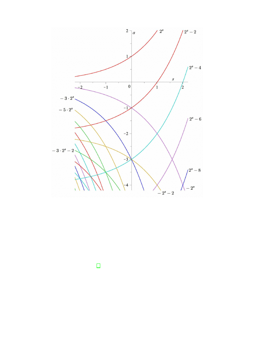
Figure 1: M

[s]

supported by monomials x

[2] I. N. Baker, “Zusammensetzungen ganzer Funktionen.” Math. Z. 69 (1958) 121–

163

[3] A. Cayley, “On some numerical expansions.” Quarterly Journal of Pure and Ap-

plied mathematics 3 (1860) 366–369. Also in: Collected Works vol. IV, pp. 470–472

[4] P. M. Cohn, Universal Algebra. Harper & Row, New York, 1965

[5] O. Costin, “Topological construction of transseries and introduction to generalized

Borel summability.” In [7], pp. 137–175

[6] O. Costin, “Global reconstruction of analytic functions from local expansions and

a new general method of converting sums into integrals.” preprint, 2007.
http://arxiv.org/abs/math/0612121

[7] O. Costin, M. D. Kruskal, A. Macintyre (eds.), Analyzable Functions and Appli-

cations (Contemp. Math. 373). Amer. Math. Soc., Providence RI, 2005

[8] L. van den Dries, A. Macintyre, D. Marker, “Logarithmic-exponential series.”

Annals of Pure and Applied Logic 111 (2001) 61–113

[9] G. Edgar, “Transseries for beginners.” Real Analysis Exchange (to appear).

http://arxiv.org/abs/0801.4877

http://www.math.ohio-state.edu/

∼edgar/preprints/trans begin/

[10] G. Edgar “Transseries: composition, recursion, and convergence.” forthcoming

http://arxiv.org/abs/0909.1259v1

http://www.math.ohio-state.edu/

∼edgar/preprints/trans compo/

[11] G. Edgar, “Transseries: ratios, grids, and witnesses.” forthcoming

http://arxiv.org/abs/0909.2430v1

http://www.math.ohio-state.edu/

∼edgar/preprints/trans wit/

[12] G. Edgar, “Tetration in transseries.” forthcoming

[13] P. Erd¨os, E. Jabotinsky, “On analytic iteration.” J. Analyse Math. 8 (1960) 361–

376

[14] J. van der Hoeven, “Operators on generalized power series.” Illinois J. Math. 45

(2001) 1161–1190

[15] J. van der Hoeven, Transseries and Real Differential Algebra (Lecture Notes in

Mathematics 1888). Springer, New York, 2006

[16] J. van der Hoeven, “Transserial Hardy fields.” preprint, 2006

[17] A. Korkine, “Sur un probl`eme d’interpolation.” Bulletin des Sciences Math´ema-

tiques et Astromomiques (2) 6 (1882) 228–242

[18] S. Kuhlmann, Ordered Exponential Fields. American Mathematical Society, Prov-

idence, RI, 2000

[19] H. F. Wilf, generatingfunctionology. Academic Press, Boston, 1990.

http://www.math.upenn.edu/~wilf/DownldGF.html

Document Outline

1 Motivation for Fractional Iteration
2 Three Examples
3 The Case of Common Support
4 Abel's Equation
5 Uniqueness
6 Julia Example

Wyszukiwarka

Podobne podstrony:
Historia gry Heroes of Might and Magic
Overview of Exploration and Production
Blanchard European Unemployment The Evolution of Facts and Ideas
Magnetic Treatment of Water and its application to agriculture
ABC Of Arterial and Venous Disease
68 979 990 Increasing of Lifetime of Aluminium and Magnesium Pressure Die Casting Moulds by Arc Ion
ABC Of Occupational and Environmental Medicine
Inequality of Opportunity and Economic Development
On The Manipulation of Money and Credit
The Hound of?ath and Other Stories
31 411 423 Effect of EAF and ESR Technologies on the Yield of Alloying Elements
21 269 287 Effect of Niobium and Vanadium as an Alloying Elements in Tool Steels
7 3 1 2 Packet Tracer Simulation Exploration of TCP and UDP Instructions
History of Jazz and Classical Music
Mock Exam? Use of English and Vocabulary
The Repentance of Compassion and Enlightenment Path
Cytotoxicity of Aqueous and Ethanolic Extracts
UTC?te and time of solstices and equinoxes

więcej podobnych podstron

Fractional Iteration of Series and Transseries G A Edgar

Document Outline