Distance-bounding facing both mafia and

distance frauds: Technical report ?

Rolando Trujillo-Rasua

1

, Benjamin Martin

2

, and Gildas Avoine

2,3

1

Interdisciplinary Centre for Security, Reliability and Trust

University of Luxembourg

2

Universit´

e catholique de Louvain

Information Security Group, Belgium

3

INSA Rennes, IRISA UMR 6074, France

Abstract. Contactless technologies such as RFID, NFC, and sensor net-
works are vulnerable to mafia and distance frauds. Both frauds aim at
passing an authentication protocol by cheating on the actual distance be-
tween the prover and the verifier. To cope these security issues, distance-
bounding protocols have been designed. However, none of the current
proposals simultaneously resists to these two frauds without requiring
additional memory and computation. The situation is even worse con-
sidering that just a few distance-bounding protocols are able to deal with
the inherent background noise on the communication channels. This ar-
ticle introduces a noise-resilient distance-bounding protocol that resists
to both mafia and distance frauds. The security of the protocol is ana-
lyzed with respect to these two frauds in both scenarios, namely noisy
and noiseless channels. Analytical expressions for the adversary’s suc-
cess probabilities are provided, and are illustrated by experimental re-
sults. The analysis, performed in an already existing framework for fair-
ness reasons, demonstrates the undeniable advantage of the introduced
lightweight design over the previous proposals.

Keywords: Authentication, distance-bounding, relay attack, mafia fraud,
distance fraud, noise.

1

Introduction

A mafia fraud is a man-in-the-middle attack applied against an authentica-

tion protocol where the adversary simply relays the exchanges without neither
manipulating nor understanding them [1]. The earliest version of this attack was
introduced by Conway in 1976 and is known as the chess grandmaster prob-
lem [5]. In this problem, a little girl is able to compete with two chess grand-
masters during a postal chess game, where she transparently relays the moves
between the two grandmasters. She eventually wins a game or draws both.

This document contains content accepted for publication at the IEEE Transactions
on Wireless Communications [18].

1

arXiv:1405.5704v1 [cs.CR] 22 May 2014

In modern cryptography, mafia frauds can typically be used against authen-

tication protocols. The adversary relays the messages between the prover and
the verifier, who think they communicate together, while there is an adversary
in the middle. This so-called mafia fraud was actually suggested by Desmedt,
Bengio and Goutier in 1987 [6] to defeat the Fiat-Shamir protocol [8].

One of the most promising field to apply the mafia fraud is the contactless

technology, especially Radio Frequency IDentification (RFID) and Near Field
Communication (NFC) where the devices answer to any solicitation without
explicit agreement of their holder. Some attacks have already been performed
against both RFID and NFC systems [10,12]. Nevertheless, mafia fraud is not
limited to contactless technologies, it also threats other technologies such as
smartcards [7] and e-voting [14].

Two other attacks related to the mafia fraud exist: the terrorist fraud and the

distance fraud. The distance fraud only involves a malicious prover, who cheats
on his distance to the verifier. It was first introduced by Brands and Chaum [4],
and comes from the distance measuring process used to defeat the mafia fraud.
The terrorist fraud is a variant of the mafia fraud where the prover is malicious
and actively helps the adversary to succeed the attack [3]. No solution exists
yet to avoid this exotic fraud, which is not addressed in this paper. Additional
countermeasure must actually be considered to thwart this fraud.

As mentioned above, a distance measuring process can mitigate the mafia

and distance frauds. To that aim, Brands and Chaum [4] proposed the distance-
bounding protocols (DB protocols). The distance estimation relies on the mea-
surement of the Round-Trip-Time (RTT) of single bit exchanges. Considering
the physical impossibility to travel faster than the speed of light, RTT bounds
the distance between the parties. Several distance-bounding protocols have been
proposed [1]. However, none of the current DB protocols are lightweight and re-
sistance to both mafia and distance frauds. Furthermore, just a few of them are
able to deal with the inherent background noise of the communication channel.

Contribution. In this paper we introduce a novel DB protocol that significantly
reduces the success probability of an adversary capable of mounting both mafia
and distance frauds. Our protocol does not rely on computationally expensive
primitives, has a very low memory requirement, and is noise-resilient. There-
fore, it is efficient and suitable for extremely low resources devices. We provide
analytical and experimental results that together show the superiority of our
proposal w.r.t. to previous ones.

Organization. Further below Section 2 presents a brief background about DB
protocols. Section 3 explains the rationality behind our proposal and Section 4
introduces and details the proposal. Sections 5 and 6 are dedicated to the re-
sistance of the protocol to mafia and distance frauds respectively. Section 7
describes our noise resiliency mechanism. Section 8 provides comparative results
with several DB protocols in both scenarios the free-noise case and the noisy
case. Finally, Section 9 draws the conclusions.

2

2

Background on distance-bounding

The first lightweight DB protocol was proposed by Hancke and Kuhn’s [11] in
2005. Its simplicity and suitability for resource-constrained devices have pro-
moted the design of other DB protocols based on it [2,13,16]. All these protocols
share the same design: (a) there is a slow phase

4

where both prover and ver-

ifier generate and exchange nonces, (b) the nonces and a keyed cryptographic
hash function are used to compute the answers to be sent (resp. checked) by
the prover (resp. verifier). Below, we provide the main characteristics of each of
these protocols, especially the technique they use to compute the answers.
Hancke and Kuhn’s protocol [11]. The answers are extracted from two n-bit
registers such that any of the n 1-bit challenges determines which register should
be used to answer.
Avoine and Tchamkerten’s protocol [2]. Binary trees are used to compute
the prover answers: the verifier challenges define the unique path in the tree,
and the prover answers are the vertex value on this path. There are several
parameters impacting the memory consumption and the resistance to distance
and mafia frauds: l the number of trees and d the depth of these trees. It holds
d · l = n, where n is the number of rounds in the fast phase. The larger d, the
better the frauds resistance and the larger the memory consumption.
Trujillo-Rasua, Martin and Avoine’s protocol [16]. This protocol is similar
to the previous one, except that it uses particular graphs instead of trees to
compute the prover answers.
Kim and Avoine’s protocol [13]. This protocol, closer to the Hancke and
Kuhn’s protocol [11] than [2] and [16], uses two registers to define the prover
answers. An important additional feature is that the prover is able to detect a
mafia fraud thanks to predefined challenges, that is, challenges known by both
prover and verifier. The number of predefined challenges impacts the frauds
resistance: the larger, the better the mafia fraud resistance, but the lower the
resistance to distance fraud.

There exist other DB protocols with different designs and computational

complexities (e.g., protocols based on signatures and/or a final extra slow phase [4,17]).
However, they are beyond the scope of this article that focuses on lightweight
protocols only. The interested reader could refer to [1] for more details.

3

Rationality of our proposal

Being resistant to both mafia and distance frauds is the primary goal of a DB
protocol. An important lower-bound for both frauds is

1
2

n

, which is the prob-

ability of a naive adversary who answers randomly to the n verifier challenges
during the fast phase. However, this resistance is hard to attain for lightweight
DB protocols. Therefore, our aim is to design a protocol that is close to this
bound for both mafia and distance frauds, without requiring costly operations

4

In DB protocols, a fast phase, which generally consists on n rounds, is a phase where
the verifier computes RTTs. Otherwise, we say that it is a slow phase.

3

or an extra final slow phase. We also aim to reach the additional property of
being noise-resilient. Below, the intuitions that lead to our design are explained
for each of the three considered properties.
Mafia fraud. Among the DB protocols without final slow phase, those achieving
the best mafia fraud resistance are round-dependent [2,13,16]. The idea is that
the correct answer at the ith round should depend on the ith challenge and also
on the (i − 1) previous challenges. Our proposal also uses a round-dependent
technique, the proposed construction is significantly simpler than those proposed
in [2,13,16], though.
Distance fraud. As in mafia fraud, the best protocols in term of distance
fraud are round-dependent. However, round-dependency by means of predefined
challenges as in the Kim and Avoine’s construction [13] fails to properly resist
to distance fraud. Intuitively, as more control over the challenges the prover has,
the lower the resistance to distance fraud is. For this reason, our proposal allows
the verifier to have full and exclusive control over the challenges.
Noise-resiliency. Round-dependent protocols can hardly work in noisy envi-
ronments. A noise in a given round might affect all the subsequent rounds and
thus, these rounds becomes useless from the security point of view. Therefore,
in order to deal with noise, round-dependent protocols should be able to detect
the noisy-rounds so that the prover responses can be checked considering these
noise occurrences. To the best of our knowledge, our protocol is the first round-
dependent DB protocol able to detect such a noisy-rounds with a high level of
accuracy thanks to the simplicity of its design.

4

Proposal

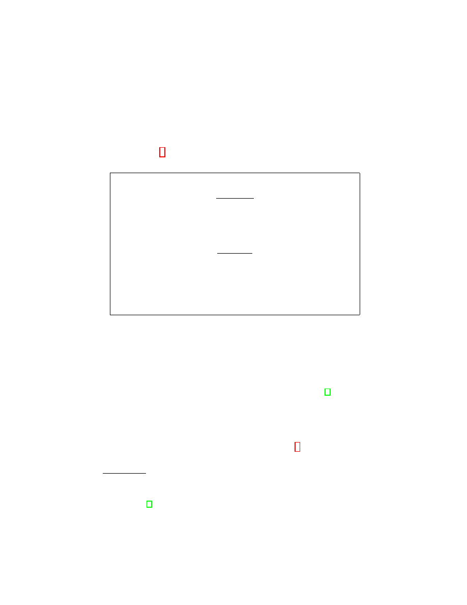
This section describes the DB protocol introduced in the paper. Initialization,
execution, and decision steps are presented below and a general view is provided
in Figure 1.

Initialization. The prover (P ) and the verifier (V ) agree on (a) a security
parameter n, (b) a timing bound ∆t

max

, (c) a pseudo random function P RF

that outputs 3n bits, (d) a secret key x.

Execution. The protocol consists of a slow phase and a fast phase.

Slow Phase. P (respectively V ) randomly picks a nonce N

P

(respectively N

V

)

and sends it to V (respectively P ). Afterwards, P and V compute P RF (x, N

P

, N

V

)

and divide the result into three n-bit registers Q, R

0

, and R

1

. Both P and V

create the function f

Q

: S → {0, 1} where S is the set of all the bit-sequences of

size at most n including the empty sequence. The function f

Q

is parameterized

with the bit-sequence Q = q

1

. . . q

n

, and it outputs 0 when the input is the empty

sequence. For every non-empty bit-sequence C

i

= c

1

. . . c

i

where 1 ≤ i ≤ n, the

function is defined as f

Q

(C

i

) =

L

i
j=1

(c

j

∧ q

j

).

4

Fast Phase. In each of the n rounds, V picks a random challenge c

i

∈

R

{0, 1},

starts a timer, and sends c

i

to P . Upon reception of c

i

, P replies with r

i

=

R

c

i

i

⊕ f

Q

(C

i

) where C

i

= c

1

...c

i

. Once V receives r

i

, he stops the timer and

computes the round-trip-time ∆t

i

.

Decision. If ∆t

i

< ∆t

max

and r

i

= R

c

i

i

⊕ f

Q

(C

i

) ∀ i ∈ {1, 2, ..., n} then the

protocol succeeds

5

.

Prover

Verifier

secret x

secret x

slow phase

picks N

P

∈

R

{0, 1}

n

picks N

V

∈

R

{0, 1}

n

N

P

−−−−−−−−−→

N

V

←−−−−−−−−−

(Q, R

0

, R

1

) = P RF (x, N

P

, N

V

)

(Q, R

0

, R

1

) = P RF (x, N

P

, N

V

)

fast phase

for i = 1, . . . , n:

picks c

i

∈

R

{0, 1}

c

i

←−−−−−−−−

start timer

r

i

= R

c

i

i

⊕ f

Q

(C

i

)

r

i

−−−−−−−−→

stop timer

computes ∆t

i

Fig. 1. Protocol description

5

Resistance to mafia fraud

Analyses of DB protocols usually consider two strategies to evaluate the resis-
tance against a mafia fraud: the pre-ask and the post-ask strategies [1]. Although
considering these two strategies only do not provide a formal security proof, this
evaluates the resistance of the protocol, at least against these well-known attack
strategies, and is the only way known so far to evaluate DB protocols. Providing
a formal security proof of DB protocols would be interesting but is clearly out
of the scope of this paper.

This section reminds the concept of pre-ask strategy

6

, then identifies the

adversarial behavior that maximizes the success probability when considering
the pre-ask strategy, and the section finally computes this probability.

5

∆t

max

is a system parameter that implicitly represents the maximum allowed dis-

tance between the prover and the verifier.

6

Note that the post-ask strategy is not relevant in protocols without an extra final
slow phase [1]

5

5.1

Best behavior

The pre-ask strategy consists first, for the adversary, to relays the initial slow
phase. Then, she runs the fast phase with the prover. With the answers she
obtains, she finally executes the fast phase with the verifier. In our case, we
consider that the adversary first sends a sequence of challenges ˜

c

1

...˜

c

n

to the

legitimate prover and receives ˜

r

1

...˜

r

n

where ˜

r

i

= R

˜

c

i

i

⊕f

Q

( ˜

C

i

) and ˜

C

i

= ˜

c

1

...˜

c

i

for

every i ∈ {1, ..., n}. Next, she executes the fast phase with the verifier receiving
the challenges c

1

...c

n

. Given ˜

r

1

...˜

r

n

, the adversarial behavior that maximizes the

success probability is provided in Theorem 1.

Theorem 1. The adversary’s behavior that maximizes her mafia fraud success
probability with a pre-ask strategy is: (a) For every round i where c

i

6= ˜

c

i

, answer

randomly. (b) For every round i where c

i

= ˜

c

i

, guess the value f

Q

(C

i

) ⊕ f

Q

( ˜

C

i

)

and answer with the value f

Q

(C

i

)⊕f

Q

( ˜

C

i

)⊕˜

r

i

where C

i

= c

1

...c

i

and ˜

C

i

= ˜

c

1

...˜

c

i

.

Proof. First, let us prove the following lemma.

Lemma 1. Given that c

i

= ˜

c

i

, the adversary’s behavior maximizing her success

probability at the ith round is equivalent to the best behavior for guessing the
value f

Q

(C

i

) ⊕ f

Q

( ˜

C

i

).

Proof. Given that c

i

= ˜

c

i

, then R

c

i

i

= R

˜

c

i

i

, which means that ˜

r

i

⊕ f

Q

( ˜

C

i

) =

r

i

⊕ f

Q

(C

i

) ⇒ r

i

= f

Q

( ˜

C

i

) ⊕ f

Q

(C

i

) ⊕ ˜

r

i

. Therefore, either the adversary guesses

f

Q

(C

i

) ⊕ f

Q

( ˜

C

i

) or the adversary losses this round.

In the case where c

i

6= ˜

c

i

, the prover’s response ˜

r

i

does not help the adversary

since R

c

i

i

and R

˜

c

i

i

are independent values. Therefore, there does not exist any

best behavior, i.e., whatever the adversary behavior, her success probability at
this round is

1
2

. This result and Lemma 1 conclude the proof.

u

t

5.2

Adversary’s success probability

Given the adversary’s behavior provided by Theorem 1, Theorem 2 provides a
recursive way to compute her success probability.

Theorem 2. Let M

i

be the event that the adversary has won the first i rounds

by following her best behavior with the pre-ask strategy. Let S

i

be the event that

the adversary guesses f

Q

(C

i

) ⊕ f

Q

( ˜

C

i

) at the ith round. The probability Pr(M

i

)

can be recursively computed as follows:

Pr(M

i

) =

1
2

i

+ Pr(M

i

|C

i

6= ˜

C

i

)

1 −

1
2

i

.

Pr(M

i

|C

i

6= ˜

C

i

) = Pr(M

i

|C

i

6= ˜

C

i

, M

i−1

)

×

1

2

i

−1

+ Pr(M

i−1

|C

i−1

6= ˜

C

i−1

)(1 −

1

2

i

−1

)

.

6

Pr(M

i

|C

i

6= ˜

C

i

, M

i−1

) = Pr(S

i−1

|C

i−1

6= ˜

C

i−1

, M

i−1

)

1 −

2

i−1

2

i

−1

+

1
2

2

i−1

2

i

−1

.

Pr(S

i

|C

i

6= ˜

C

i

, M

i

) =

1
2

+

1
2

Pr(S

i−1

|M

i−1

,C

i−1

6= ˜

C

i−1

) Pr(M

i−1

|C

i−1

6= ˜

C

i−1

)

1−

(

1
2

)

i−1

1
2

Pr(M

i

|C

i

6= ˜

C

i

)

1−

(

1
2

)

i

.

Where Pr(M

1

|C

1

6= ˜

C

1

) = 1/2 and Pr(S

1

|C

1

6= ˜

C

1

, M

1

) = 1/2 are the stopping

conditions.

Proof. If C

i

= ˜

C

i

, the adversary knows that f

Q

(C

i

) ⊕ f

Q

( ˜

C

i

) = 0 and thus, her

success probability until the ith round is 1, which means that Pr(M

i

|C

i

= ˜

C

i

) =

1. Considering that Pr(C

i

= ˜

C

i

) = (1/2)

i

and Pr(C

i

6= ˜

C

i

) = 1 − (1/2)

i

, then

Pr(M

i

) can be expressed as follows:

Pr(M

i

) =

1

2

i

+ Pr(M

i

|C

i

6= ˜

C

i

)

1 −

1

2

i

!

.

(1)

Equation 1 states that the computation of Pr(M

i

) requires Pr(M

i

|C

i

6= ˜

C

i

).

Note that M

i

holds if M

i−1

holds, so:

Pr(M

i

|C

i

6= ˜

C

i

) = Pr(M

i

|C

i

6= ˜

C

i

, M

i−1

) Pr(M

i−1

|C

i

6= ˜

C

i

).

(2)

Given that M

i−1

depends on whether C

i−1

= ˜

C

i−1

or not, and considering

that Pr(C

i−1

= ˜

C

i−1

|C

i

6= ˜

C

i

) = 1/(2

i

− 1), then Pr(M

i−1

|C

i

6= ˜

C

i

) can be

transformed as follows:

Pr(M

i−1

|C

i

6= ˜

C

i

)

= Pr(M

i−1

|C

i

6= ˜

C

i

, C

i−1

= ˜

C

i−1

) Pr(C

i−1

= ˜

C

i−1

|C

i

6= ˜

C

i

)

+ Pr(M

i−1

|C

i

6= ˜

C

i

, C

i−1

6= ˜

C

i−1

) Pr(C

i−1

6= ˜

C

i−1

|C

i

6= ˜

C

i

)

=

1

2

i

− 1

+ Pr(M

i−1

|C

i−1

6= ˜

C

i−1

)

2

i

− 2

2

i

− 1

.

(3)

Assuming that Pr(M

i

|C

i

6= ˜

C

i

, M

i−1

) can be computed for every i, then ac-

cording to Equations 2 and 3, Pr(M

i

|C

i

6= ˜

C

i

) can be recursively computed as

follows:

Pr(M

i

|C

i

6= ˜

C

i

) = Pr(M

i

|C

i

6= ˜

C

i

, M

i−1

)

×

1

2

i

− 1

+ Pr(M

i−1

|C

i−1

6= ˜

C

i−1

)

2

i

− 2

2

i

− 1

.

(4)

Note that, the result Pr(M

1

|C

1

6= ˜

C

1

) = 1/2 can be used as the stopping condi-

tion for the recursion defined in Equation 4. This recursion simplifies the analy-
sis of Pr(M

i

): instead of analyzing the probability to win all the i rounds, only

7

the probability to win the ith round is needed. Since it depends on the adver-
sary’s behavior, and the latter depends on whether c

i

= ˜

c

i

or not, we compute

Pr(M

i

|C

i

6= ˜

C

i

, M

i−1

) as follows:

Pr(M

i

|C

i

6= ˜

C

i

, M

i−1

) =

Pr(M

i

|C

i−1

6= ˜

C

i−1

, M

i−1

, c

i

= ˜

c

i

) Pr(c

i

= ˜

c

i

|C

i

6= ˜

C

i

)

+ Pr(M

i

|C

i

6= ˜

C

i

, M

i−1

, c

i

6= ˜

c

i

) Pr(c

i

6= ˜

c

i

|C

i

6= ˜

C

i

).

(5)

When c

i

6= ˜

c

i

the adversary answers randomly and thus Pr(M

i

|C

i

6= ˜

C

i

, M

i−1

, c

i

6=

˜

c

i

) = 1/2. Considering this result and that Pr(c

i

6= ˜

c

i

|C

i

6= ˜

C

i

) = 2

i−1

/(2

i

− 1),

Equation 5 yields to:

Pr(M

i

|C

i

6= ˜

C

i

, M

i−1

) =

2

i−2

2

i

− 1

+ Pr(M

i

|C

i−1

6= ˜

C

i−1

, M

i−1

, c

i

= ˜

c

i

)

1 −

2

i−1

2

i

− 1

.

(6)

From Equation 6, we deduce that computing Pr(M

i

) requires Pr(M

i

|C

i−1

6=

˜

C

i−1

, M

i−1

, c

i

= ˜

c

i

). Theorem 2 states that the adversary’s behavior in this case

is to guess f

Q

(C

i

) ⊕ f

Q

( ˜

C

i

). Hence:

Pr(M

i

|C

i−1

6= ˜

C

i−1

, M

i−1

, c

i

= ˜

c

i

) = Pr(S

i

|C

i−1

6= ˜

C

i−1

, M

i−1

, c

i

= ˜

c

i

)

(7)

We now aim at computing Pr(S

i

|C

i−1

6= ˜

C

i−1

, M

i−1

, c

i

= ˜

c

i

). Since c

i

= ˜

c

i

, then

f

Q

(C

i

) ⊕ f

Q

( ˜

C

i

) = f

Q

(C

i−1

) ⊕ f

Q

( ˜

C

i−1

). Therefore, the adversary’s strategy

maximizing Pr(S

i

|C

i−1

6= ˜

C

i−1

, M

i−1

, c

i

= ˜

c

i

) consists in holding her previous

guess for the (i − 1)th round. So:

Pr(S

i

|C

i−1

6= ˜

C

i−1

, M

i−1

, c

i

= ˜

c

i

) = Pr(S

i−1

|C

i−1

6= ˜

C

i−1

, M

i−1

).

(8)

As pointed out by Equation 8 and Equation 7, computing Pr(M

i

|C

i−1

6= ˜

C

i−1

, M

i−1

, c

i

=

˜

c

i

) requires Pr(S

i−1

|C

i−1

6= ˜

C

i−1

, M

i−1

). Since it is indexed by i − 1, we assume

that Pr(M

j

) is already computed for every j < i and as shown by Lemma 2,

Pr(S

i−1

|C

i−1

6= ˜

C

i−1

, M

i−1

) can be recursively computed.

Lemma 2. Given that Pr(M

j

|C

j

6= ˜

C

j

) can be computed for every j ≤ i, then

Pr(S

i

|C

i

6= ˜

C

i

, M

i

) can be recursively computed as follows:

Pr(S

i

|C

i

6= ˜

C

i

, M

i

) =

1

2

+

Pr(S

i−1

|M

i−1

, C

i−1

6= ˜

C

i−1

)

Pr(M

i

|C

i

6= ˜

C

i

)

1 −

1
2

i

× Pr(M

i−1

|C

i−1

6= ˜

C

i−1

)

1

2

−

1

2

i

!

.

where Pr(S

1

|C

1

6= ˜

C

1

, M

1

) =

1
2

is the stopping condition.

8

Proof. By definition of f

Q

(.), and because Pr(q

i

= 0) = Pr(q

i

= 1) = 1/2,

Pr(S

i

|C

i

6= ˜

C

i

, M

i

, c

i

6= ˜

c

i

) = 1/2. Moreover, Theorem 1 states that M

i

and S

i

are equivalent when c

i

= ˜

c

i

, hence Pr(S

i

|C

i

6= ˜

C

i

, M

i

, c

i

= ˜

c

i

) = 1. Considering

both results we obtain:

Pr(S

i

|C

i

6= ˜

C

i

, M

i

) =

1

2

+

1

2

Pr(c

i

= ˜

c

i

|C

i

6= ˜

C

i

, M

i

).

(9)

Finally, considering that Pr(C

i

6= ˜

C

i

) = 1 −

1
2

i

and Pr(c

i

= ˜

c

i

, C

i

6= ˜

C

i

) =

1 −

1
2

i−1

1
2

, the probability Pr(c

i

= ˜

c

i

|C

i

6= ˜

C

i

, M

i

) can be expressed as

follows:

Pr(c

i

= ˜

c

i

|C

i

6= ˜

C

i

, M

i

) =

Pr(c

i

= ˜

c

i

, C

i

6= ˜

C

i

, M

i

, M

i−1

)

Pr(C

i

6= ˜

C

i

, M

i

)

=

Pr(M

i

|M

i−1

, c

i

= ˜

c

i

, C

i

6= ˜

C

i

)

Pr(M

i

|C

i

6= ˜

C

i

) Pr(C

i

6= ˜

C

i

)

× Pr(M

i−1

|c

i

= ˜

c

i

, C

i

6= ˜

C

i

) Pr(c

i

= ˜

c

i

, C

i

6= ˜

C

i

)

=

Pr(S

i−1

|M

i−1

, C

i−1

6= ˜

C

i−1

)

Pr(M

i

|C

i

6= ˜

C

i

)

1 −

1
2

i

(10)

× Pr(M

i−1

|C

i−1

6= ˜

C

i−1

)

1

2

−

1

2

i

!

.

Equations 9 and 10 yield the expected result.

Lemma 2 together with Equations 1, 4, 6, 7, and 8, conclude the proof of this
theorem.

6

Resistance to distance fraud

This section analyzes the adversary success probability when mounting a dis-
tance fraud. As stated in [1], the common way to analyze the resistance to
distance fraud is by considering the early-reply strategy instead of the pre-ask
strategy. This strategy consists on sending the responses in advance, i.e., before
receiving the challenges. Doing so, the adversary gains some time and might pass
the timing constraint. In this section, the behavior that maximizes the success
probability using the early-reply strategy is identified, and then a recursive way
to compute the resistance w.r.t. a distance fraud is provided.

6.1

Best behavior

With the early-reply strategy, in order to send a response in advance in the ith
round with probability of being correct greater that 1/2, the adversary must

9

send either R

0
i

⊕ f

Q

(C

i−1

||0) or R

1
i

⊕ f

Q

(C

i−1

||1) where C

i−1

is the sequence of

challenges sent by the verifier until the (i − 1)th round. Theorem 3 shows that,
guessing the values f

Q

(C

i

) for every i ∈ {1, ..., n − 1} is needed to maximize the

adversary success probability.

Theorem 3. Let C

i

be the sequence of challenges c

1

...c

i

sent by the verifier until

the ith round (i ≥ 1). The adversary’s behavior that maximizes her distance fraud
success probability is equivalent to the best behavior for guessing the values
f

Q

(C

1

), f

Q

(C

2

), ..., f

Q

(C

n−1

).

Proof. In order to send a response in advance at the ith round with proba-
bility of being correct greater that 1/2, the adversary must send either R

0
i

⊕

f

Q

(C

i−1

||0) or R

1
i

⊕ f

Q

(C

i−1

||1). By definition, f

Q

(C

i−1

||0) = f (C

i−1

) and

f

Q

(C

i−1

||1) = f

Q

(C

i−1

) ⊕ q

i

. Therefore, R

0
i

⊕ f

Q

(C

i−1

||0) = R

0
i

⊕ f

Q

(C

i−1

)

and R

1
i

⊕ f

Q

(C

i−1

||1) = R

1
i

⊕ f

Q

(C

i−1

) ⊕ q

i

. Since the adversary knows the

values R

0
i

, R

1
i

, and q

i

, guessing the correct value at this round is equivalent to

guessing the correct value of f

Q

(C

i−1

).

As stated in Theorem 3, computing the adversary success probability re-

quires the best behavior to guess the outputs sequence f

Q

(C

1

), . . . , f

Q

(C

n−1

).

Theorem 4 solves this problem.

Theorem 4. The best adversary’s behavior to guess f

Q

(C

i

) is to assume that

her previous guess for f

Q

(C

i−1

) is correct and to compute f

Q

(C

i

) as follows: (a)

if q

i

= 0, then consider f

Q

(C

i

) = f

Q

(C

i−1

). (b) if q

i

= 1, pick a random bit c

i

and consider that f

Q

(C

i

) = f

Q

(C

i−1

) ⊕ c

i

.

Proof. Assuming that q

i

= 0, then f

Q

(C

i

) = f

Q

(C

i−1

) and thus, the probability

to guess f

Q

(C

i

) is equal to the probability of guessing f

Q

(C

i−1

). In the case of

q

i

= 1, the adversary does not have a better behavior than choosing a random

bit of challenge c

i

and considering that f

Q

(C

i

) = f

Q

(C

i−1

) ⊕ c

i

. Given that

f

Q

() = 0 where is the empty sequence, the proof can be straightforwardly

concluded by induction.

6.2

Adversary’s success probability

Given the best adversary’s behavior provided by Theorems 3 and 4, Theorem 5
shows a recursive way to compute the resistance to distance fraud.

Theorem 5. Let D

i

be the event that the distance fraud adversary successfully

passes the protocol until the ith round. Then, Pr(D

i

) can be computed as follows:

Pr(D

i

) =

1

4

Pr(D

i−1

) +

1

2

i

+

1

8

i−1

X

j=1

Pr(D

j

)

1

2

i−j

.

where Pr(D

0

) = 1 is the stopping condition.

10

Proof. Let F

i

be the event that the adversary correctly guesses the value of

f

Q

(C

i

). Then, the event D

i

depends on the events D

i−1

and F

i−1

, which can be

expressed as follows:

Pr(D

i

) = Pr(D

i

|D

i−1

, F

i−1

) Pr(D

i−1

, F

i−1

)

+ Pr(D

i

|D

i−1

, ¯

F

i−1

) Pr(D

i−1

, ¯

F

i−1

).

(11)

Two cases occur (a) R

0
i

= R

1
i

and (b) R

0
i

6= R

1
i

. In the first case, the ad-

versary wins the ith round if and only if she guesses the value f

Q

(C

i−1

), so

Pr(D

i

|D

i−1

, F

i−1

, R

0
i

= R

1
i

) = 1 and Pr(D

i

|D

i−1

, ¯

F

i−1

, R

0
i

= R

1
i

) = 0. In the

second case, the adversary has no better probability to win than 1/2 and thus,
Pr(D

i

|D

i−1

, F

i−1

, R

0
i

6= R

1
i

) = Pr(D

i

|D

i−1

, ¯

F

i−1

, R

0
i

6= R

1
i

) = 1/2. Therefore,

we deduce Pr(D

i

|D

i−1

, F

i−1

) = 3/4 and Pr(D

i

|D

i−1

, ¯

F

i−1

) = 1/4. Using these

results and Equation 11 we have:

Pr(D

i

) =

3

4

Pr(D

i−1

, F

i−1

) +

1

4

Pr(D

i−1

, ¯

F

i−1

)

=

1

4

Pr(D

i−1

) +

1

2

Pr(D

i−1

, F

i−1

).

(12)

Equation 12 states that Pr(D

i

) can be computed by recursion if we express

Pr(D

i−1

, F

i−1

) in terms of the events D

j

where 1 ≤ j < i. Therefore, in the

remaining of this proof we aim at looking for such result. As above, in order to
analyze Pr(D

i

, F

i

), the events D

i−1

and F

i−1

should be considered:

Pr(D

i

, F

i

) = Pr(D

i

|F

i

, D

i−1

, F

i−1

) Pr(F

i

|D

i−1

, F

i−1

) Pr(D

i−1

, F

i−1

)

+ Pr(D

i

|F

i

, D

i−1

, ¯

F

i−1

) Pr(F

i

|D

i−1

, ¯

F

i−1

) Pr(D

i−1

, ¯

F

i−1

).

(13)

Four cases should be analyzed depending on the value of q

i

and the events F

i

and F

i−1

.

Case 1 (q

i

= 1, F

i

and F

i−1

hold). This case occurs if the adversary correctly

guesses the challenge c

i

. Therefore, she provides the correct answer at this round

R

c

i

i

⊕ f

Q

(C

i

). So, Pr(D

i

|F

i

, D

i−1

, F

i−1

, q

i

= 1) = 1.

Case 2 (q

i

= 1, F

i

and ¯

F

i−1

hold). Given that ¯

F

i−1

and F

i

hold, the adversary

computed f

Q

(C

i

) = f

Q

(C

i−1

) ⊕ ˜

c

i

using a challenge different from the verifier’s

one, i.e., c

i

6= ˜

c

i

. Therefore, Pr(D

i

|F

i

, D

i−1

, ¯

F

i−1

, q

i

= 1) =

1
2

because both

events F

i

and ¯

F

i−1

coexist only if q

i

= 1, then Pr(q

i

= 1|F

i

, D

i−1

, ¯

F

i−1

) = 1.

Case 3 (q

i

= 0, F

i

and F

i−1

hold). Given q

i

= 0, the event F

i

has no effect on the

event D

i

. Thus, Pr(D

i

|F

i

, D

i−1

, F

i−1

, q

i

= 0) = Pr(D

i

|D

i−1

, F

i−1

, q

i

= 0) =

3
4

because it depends on whether R

0
i

= R

1
i

. So, Pr(D

i

|F

i

, D

i−1

, F

i−1

, q

i

= 0) =

3
4

.

Case 4 (q

i

= 0, F

i

and ¯

F

i−1

hold). When q

i

= 0, then f

Q

(C

i

) = f

Q

(C

i−1

), which

means that this case cannot occur. Therefore, Pr(F

i

, D

i−1

, ¯

F

i−1

, q

i

= 0) = 0.

11

Cases 1 and 3 yield the following result:

Pr(D

i

|F

i

, D

i−1

, F

i−1

) = Pr(q

i

= 1|F

i

, D

i−1

, F

i−1

) +

3

4

Pr(q

i

= 0|F

i

, D

i−1

, F

i−1

)

=

3

4

−

1

4

Pr(q

i

= 1|F

i

, D

i−1

, F

i−1

).

(14)

And Cases 2 and 4 yield this other result:

Pr(D

i

|F

i

, D

i−1

, ¯

F

i−1

) =

1

2

.

(15)

Because Pr(F

i

|F

i−1

, q

i

= 0) = 1 and Pr(F

i

|F

i−1

, q

i

= 1) = 1/2, we have

Pr(F

i

|D

i−1

, F

i−1

) = Pr(F

i

|F

i−1

) = 3/4. Similarly, Pr(F

i

|D

i−1

, ¯

F

i−1

) = Pr(F

i

| ¯

F

i−1

) =

1/4 because Pr(F

i

| ¯

F

i−1

, q

i

= 0) = 0 and Pr(F

i

| ¯

F

i−1

, q

i

= 1) = 1/2. Combining

these results with Equations 14 and 15, Equation 13 becomes:

Pr(D

i

, F

i

) =

3

4

−

1

4

Pr(q

i

= 1|F

i

, D

i−1

, F

i−1

)

3

4

Pr(D

i−1

, F

i−1

)

+

1

2

1

4

Pr(D

i−1

, ¯

F

i−1

)

=

3

16

Pr(q

i

= 1|F

i

, D

i−1

, F

i−1

) Pr(D

i−1

, F

i−1

) +

9

16

Pr(D

i−1

, F

i−1

)

+

1

8

Pr(D

i−1

, ¯

F

i−1

)

=

3

16

Pr(q

i

= 1, F

i

, D

i−1

, F

i−1

)

Pr(F

i

|D

i−1

, F

i−1

)

+

9

16

Pr(D

i−1

, F

i−1

) +

1

8

Pr(D

i−1

, ¯

F

i−1

)

=

3

16

Pr(F

i

|q

i

= 1, D

i−1

, F

i−1

) Pr(D

i−1

, F

i−1

)

1
2

Pr(F

i

|D

i−1

, F

i−1

)

+

9

16

Pr(D

i−1

, F

i−1

)

+

1

8

Pr(D

i−1

, ¯

F

i−1

)

=

3

16

1
2

Pr(D

i−1

, F

i−1

)

1
2

3
4

+

9

16

Pr(D

i−1

, F

i−1

) +

1

8

Pr(D

i−1

, ¯

F

i−1

)

=

1

16

Pr(D

i−1

, F

i−1

) +

9

16

Pr(D

i−1

, F

i−1

) +

1

8

Pr(D

i−1

, ¯

F

i−1

)

=

5

8

Pr(D

i−1

, F

i−1

) +

1

8

(Pr(D

i

) − Pr(D

i−1

, F

i−1

))

=

1

2

Pr(D

i−1

, F

i−1

) +

1

8

Pr(D

i

)

=

1

2

i

+

1

8

i

X

j=1

Pr(D

j

)

1

2

i−j

.

(16)

Considering that Pr(D

0

) = 1, Equations 16 and 12 yield the expected result.

12

7

Noise resilience

Some efforts have been made in order to adapt existing distance-bounding pro-
tocols to noisy channels. Most of them rely on using a threshold x representing
the maximum number of incorrect responses expected by the verifier [11,13].
Intuitively, the larger x, the lower the false rejection ratio but also the lower
the resistance to mafia and distance frauds. Others use an error correction code
during an extra slow phase [17]. However, the latter cannot be applied to our
protocol given that it does not contain any final slow phase. Consequently, we
focus on the threshold technique.

7.1

Understanding the noise effect in our protocol

We consider in the analysis that a 1-bit challenge (on the forward channel)
can be flipped due to noise with probability p

f

and a 1-bit answer (on the

backward channel) can be flipped with probability p

b

. Further, we denote as

˜

c

i

the bit-challenge received by the prover at the ith round, which might be

obviously different to the challenge c

i

. Similarly, ˜

r

i

denotes the response received

by the verifier at the ith round. As in previous works [11], the considered forward
and backward channels are assumed to be memoryless. Table 1 shows the three
different scenarios when considering a noisy communication at the i-th round in
our protocol.

Forward Noise

Backward Noise

Forward and
Backward Noise

P receives ˜

c

i

= c

i

⊕ 1

P receives ˜

c

i

= c

i

P receives ˜

c

i

= c

i

⊕ 1

P updates ˜

C

i

= ˜

c

1

...˜

c

i

P updates ˜

C

i

= ˜

c

1

...˜

c

i

P updates ˜

C

i

= ˜

c

1

...˜

c

i

P sends r

i

= R

˜

c

i

i

⊕ f

Q

( ˜

C

i

) P sends R

c

i

i

⊕ f

Q

( ˜

C

i

) P sends R

˜

c

i

i

⊕ f

Q

( ˜

C

i

)

V receives ˜

r

i

= r

i

V receives ˜

r

i

= r

i

⊕ 1 V receives ˜

r

i

= r

i

⊕ 1

Table 1. The three possible scenarios when some noise occurs at the ith round.

According to the protocol, in a noise-free ith round executed with a legitimate

prover it holds that r

i

= ˜

r

i

⇔ f

Q

(C

i

) = f

Q

( ˜

C

i

). We thus say that prover and

verifier are synchronized at the ith round if f

Q

(C

i

) = f

Q

( ˜

C

i

), otherwise they are

said to be desynchronized. Intuitively, in a noise-free ith round the answer ˜

r

i

can

be considered correct by the verifier either if r

i

= ˜

r

i

and they are synchronized

or if r

i

6= ˜

r

i

and they are desynchronized.

The challenge is therefore to identify whether the prover and the verifier are

synchronized or not. To that aim, we rise the following observation.

Observation 1 Several consecutive rounds where all, or almost all, the answers
hold that r

i

= ˜

r

i

(resp. r

i

6= ˜

r

i

), might indicate that the legitimate prover and

the verifier have been synchronized (resp. desynchronized).

13

7.2

Our noise resilient mechanism

Based on Observation 1, we propose an heuristic aimed at identifying those
rounds where prover and verifier switch from being synchronized to desynchro-
nized or vice versa. The heuristic is named SwitchedRounds and its pseudocode
description is provided by Algorithm 1.

SwitchedRounds creates first the sequence d

1

...d

n

where d

i

= 0 if r

i

= ˜

r

i

,

otherwise d

i

= 1. Following Observation 1, it searches for the longest subsequence

d

i

...d

j

that matches any of the following patterns

7

: (a) ∧(1+)0 (b) ∧(1+)$ (c)

1(0+)1 (d) 0(1+)0 (e) 1(0+)$ (f) 0(1+)$.

The aim of these patterns is to look for large subsequences of either consec-

utive 0s or 1s in d

1

. . . d

n

. Note that, we do not include the patterns ∧(0+)1 and

∧(0+)$ because starting with a sequence of zeros is exactly what the verifier
expects. Intuitively, the lower the expected noise the larger the subsequences
should be. As an example, let us consider the case where the communication
channel is noiseless. Since no noise is expected, the sequence d

1

. . . d

n

should be

equal to n consecutive zeros unless an attack is being performed. In Algorithm 1,
a threshold ∆l defines how large a matching d

i

...d

j

should be in order to be an-

alyzed. We discuss a computational approach to estimate a practical value for
∆l in Section 8.

If a pattern d

i

...d

j

holds that j − i ≥ ∆l, SwitchedRounds looks for the closer

index r to i + 1 such that q

r

= 1, and assumes that the rth round caused the

switch from synchronization to desynchronization or vice versa. To understand
this choice, let us note that a pattern d

i

...d

j

implies that d

i

6= d

i+1

. This could

have happened if a switch from synchronization to desynchronization or vice
versa occurred in the (i + 1)th round. However, due to the probabilistic nature
of the noise we cannot precisely determine whether the switch occurred in the
(i + 1)th round or in some (possibly close) round. What we do know is that such
a round r must hold that q

r

= 1, which justifies Step 5 in Algorithm 1.

Once r is found, the pair (r, s) is created where s is 0 if the switch is to

synchronization, s = 1 otherwise. Finally, SwitchedRounds recursively calls itself
to analyze the two subsequences lying on the left and right side of d

i

...d

j

. The

output is the union of all obtained pairs such that they are in increasing order
(according to the round) and every two consecutive pairs have different values
(according to the type of switching).

Armed with the SwitchedRounds algorithm, the threshold technique can be

straightforwardly applied as Algorithm 2 shows. It simply counts the number of
errors occurred during the execution of the protocol where an error is defined as
either a switched round or a wrong response. Both cases are considered as error
because, on the one hand, a switched round might be falsely detected during an
attack, and on the other hand, there is no distinction between a wrong response
due to noise or to an attack. Finally, the protocol is considered to fail if the
number of errors is above a threshold x.

7

The patterns have been written following the POSIX Extended Regular Expres-
sions standard. The symbols ∧ and $ represent the start and the end of the string
respectively.

14

Algorithm 1 SwitchedRounds

Require: The challenges c

1

...c

n

and the registers R

0

, R

1

, and Q. The prover’s re-

sponses ˜

r

1

...˜

r

n

. A threshold ∆l indicating the minimum matching length.

1: Let d

1

...d

n

be a sequence such that d

i

= ˜

r

i

⊕ R

c

i

i

⊕ f (C

i

).

2: Let

d

i

...d

j

be

the

longest

matching

with

∧(1+)0|

∧

(1+)$|0(1+)0|0(1+)$|1(0+)1|1(0+)$ on d

1

...d

n

.

3: if j − i < ∆l or no matching exists then return the empty set;

4: Let s be 0 if the matching is with 1(0+)1|1(0+)$ and 1 otherwise;
5: Let r be the closest index to i + 1 such that q

r

= 1;

6: Let A be the output of SwitchedRounds on d

1

...d

i−1

;

7: Let B be the output of SwitchedRounds on d

j+1

...d

n

;

8: Let E be the union of A ∪ {(r, s)} ∪ B such that the indexes are in increasing order

and every two consecutive pairs have different boolean values;

9: return E;

Note that basing the decision on a threshold is a common and easy procedure

but not the best one, especially when the channels are not memoryless. Instead,
the decision procedure could consist in comparing the vector d

1

...d

n

with the

error distribution on the noisy channels.

Algorithm 2 Authentication in the presence of noise

Require: All the parameters of the protocol; an integer value x representing the noise

tolerance; and a threshold ∆l.

1: Let E be the output of SwitchedRounds algorithm on input c

1

...c

n

, ˜

r

1

...˜

r

n

, R

0

, R

1

,

Q, and ∆l;

2: Let d

1

...d

n

be a sequence such that d

i

= ˜

r

i

⊕ R

c

i

i

⊕ f (C

i

).

3: Let s be a boolean variable initialized in 0;
4: Let errors be a counter initialized in 0;
5: for all 1 ≤ i ≤ n do
6:

if (i, s

0

) ∈ E then

7:

s ← s

0

;

8:

errors + +;

9:

else if (d

i

= 0 and s = 1) or (d

i

= 1 and s = 0) then

10:

errors + +;

11: if errors > x then return fail;
12: else return success;

8

Experiments and comparison

The first part of this section is devoted to compare several DB protocols in term
of mafia fraud resistance, distance fraud resistance, and memory consumption.
The second part takes noise into account and evaluates our proposal w.r.t. the
Hancke and Kuhn’s [11] and Kim and Avoine’s [13] protocols.

15

8.1

Noise-free environment

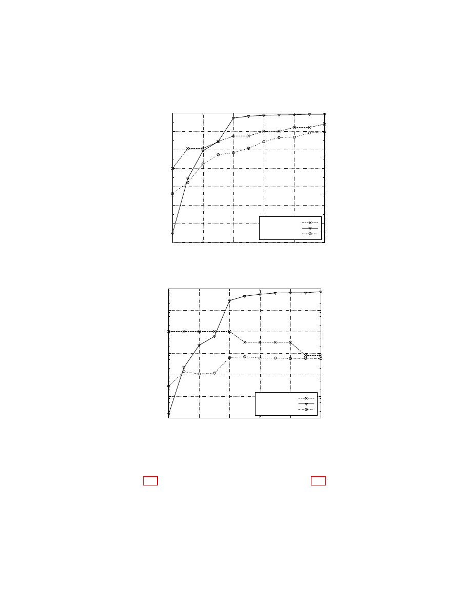
Mafia and distance fraud analyses in a noise-free environment can be found
in [11,13,16,2] for KA2, AT, Poulidor, and HK. In the case of AT and Pouli-
dor, only an upper-bound of their resistance to distance fraud have been pro-
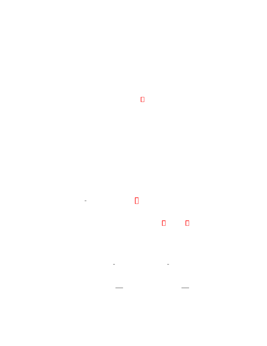
vided [16,9]. Considering those previous results, Fig. 2(a) and Fig. 2(b) show the
resistance to mafia and distance frauds respectively for the five considered pro-
tocols in a single chart. For each of them, the configuration that maximizes its
security has been chosen: this is particularly important for AT and KA2 because
different configurations can be used.

Figures 2(a) and 2(b) show that AT and KA2 are the best protocols in terms

of mafia fraud while our proposal is the best in terms of distance fraud. However,
it makes sense to consider the two properties together. To do so, we follow the
technique used in [16] to seek for a good trade-off. This technique first discretizes
the mafia fraud (x) and distance fraud (y) success probabilities. For every pair
(x, y), it then evaluates which protocol is the less round-consuming. This protocol
is considered as the best for the considered pair. In case of draw between two
protocols, the one that is the less memory-consuming is considered as the best
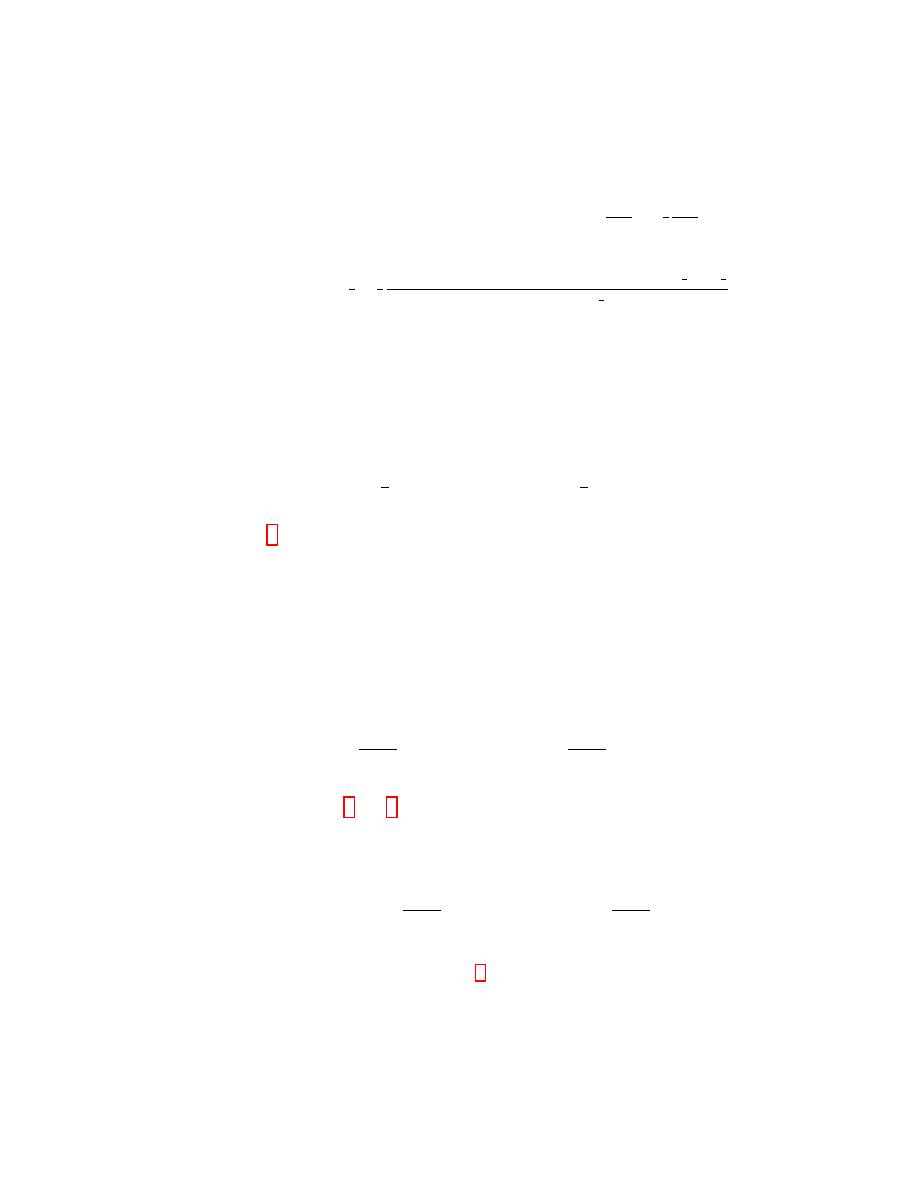
protocol. Using this idea, it is possible to draw what we call a trade-off chart,
which represents for every pair (x, y) the best protocol among the five considered
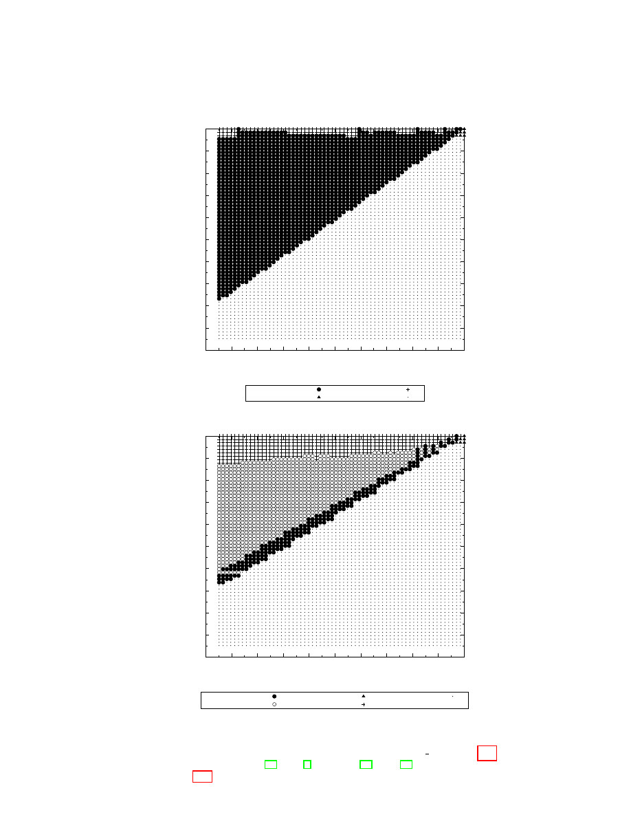
(see Figure 3(a)).

Figure 3(a) shows that our protocol offers a good trade-off between resistance

to mafia fraud and resistance to distance fraud, especially when a high security
level against distance fraud is expected. In other words, our protocol defeats all
the other considered protocols, except when the expected security levels for mafia
and distance fraud are unbalanced, which is meaningless in common scenarios.

Another interesting comparison could take into consideration the memory

consumption of the protocols. Indeed, for n rounds of the fast phase, AT requires
2

n+1

− 1 bits of memory, which is prohibitive for most pervasive devices. We can

therefore compare protocols that require a linear memory w.r.t. the number
of rounds n. For that, we consider a variant of AT [2], denoted AT-3, that
uses n/3 trees of depth 3 instead of just one tree of depth n. By doing so, the
memory consumption of all the considered protocols is below 5n bits of memory.
The resulting trade-off chart (Figure 3(b)) shows that constraining the memory
consumption considerable reduces the area where AT is the best protocol, but
it also shows that our protocol is also the best trade-off in this scenario.

8.2

Noisy environment

Among the protocols we are considering, only HK [11] and KA2 [13] claim to
be noise resilient. For this reason, we analyze in this section the performance of
our proposal in the presence of noise by comparing it with HK and KA2. The
comparison is performed by considering two properties: availability and security.
Availability is measured in terms of false rejection ratio and security in terms
of mafia fraud resistance. It should be remarked that, distance fraud resistance

16

1e-018

1e-016

1e-014

1e-012

1e-010

1e-008

1e-006

0.0001

0.01

1

1

10

64

Adversary Success Probability

Rounds

AT and KA2

Poulidor

Our proposal

HK

(a) Mafia Fraud

1e-012

1e-010

1e-008

1e-006

0.0001

0.01

1

1

10

64

Adversary Success Probability

Rounds

Our proposal

AT

HK and KA2

Poulidor

(b) Distance Fraud

Fig. 2. The mafia fraud (Figure 2(a)) and distance fraud (Figure 2(b)) success proba-
bilities considering up to 64 rounds (logarithmic scale). The considered protocols are
KA2 [13], AT [2], Poulidor [16], HK [11], and our protocol.

17

1e-020

1e-018

1e-016

1e-014

1e-012

1e-010

1e-008

1e-006

0.0001

0.01

1

1e-020 1e-018 1e-016 1e-014 1e-012 1e-010 1e-008 1e-006 0.0001 0.01

1

Distance Fraud

Mafia fraud

AT

HK

KA2

Our proposal

(a) Trade-off without memory constraint

1e-020

1e-018

1e-016

1e-014

1e-012

1e-010

1e-008

1e-006

0.0001

0.01

1

1e-020 1e-018 1e-016 1e-014 1e-012 1e-010 1e-008 1e-006 0.0001 0.01

1

Distance Fraud

Mafia fraud

AT-3

Poulidor

HK

KA2

Our proposal

(b) Trade-off with memory constraint

Fig. 3. Two trade-off charts showing the most efficient protocol for each pair of mafia
fraud and distance fraud probability values ranging between 1 and

1
2

64

. Figure 3(a)

considers the protocols KA2 [13], AT [2], Poulidor [16], HK [11], and our proposal,
while Figure 3(b) changes AT by its low-resource consuming variant AT-3.

18

has not been considered for simplicity and because, as shown previously, our
proposal outperforms all the other protocols in terms of this fraud.

An important parameter when measuring availability and security for the

three protocols is the number of allowed incorrect responses (x). In the case of
KA2 and our proposal, other parameters are the minimum size of the pattern
(s) (denoted by ∆l in Algorithm 1) and the number of predefined challenges
p respectively. Theoretical bounds for these parameters in term of the number
of rounds and noise probabilities might be provided, however, we left this non-
trivial task for future work. Instead, we treat the three parameters z = (x, s, p)
as the variables of an optimization problem defined as follows:

Problem 1. Let Π be a distance-bounding protocol, n the number of rounds, p

f

the probability of noise in the forward channel, and p

b

the probability of noise

in the backward channel. Let Π

security

p

f

,p

b

,n

(z) and Π

availability

p

f

,p

b

,n

(z) be the functions

that, given a set of parameters z = (x, s, p), compute the adversary success
probability when mounting a mafia fraud against Π and the false rejection ration
of Π respectively. Given a threshold ∆, the optimization problem consists in:

minimizing

Π

security

p

f

,p

b

,n

(z)

subject to

Π

availability

p

f

,p

b

,n

(z) ≤ ∆

To follow notations of Problem 1, we assume that Π ∈ {HK, KA2, Our}

where “Our” denotes our proposal. Therefore, algorithms to compute Π

security

p

f

,p

b

,n

(z)

and Π

availability

p

f

,p

b

,n

(z) for every Π ∈ {HK, KA2, Our} are required. In case Π =

HK, HK

security
p

f

,p

b

,n

(z) can be computed as shown in [11], while HK

availability
p

f

,p

b

,n

(z) is

provided by Theorem 6 (see Appendices). For Π = KA2, an algorithm to com-
pute KA2

security
p

f

,p

b

,n

(z) is given in [13]. Unfortunately, analytical expressions for

KA2

availability
p

f

,p

b

,n

(z), Our

security
p

f

,p

b

,n

(z), and Our

availability
p

f

,p

b

,n

(z), seem to be cumbersome

to find. Therefore, we address this issue by means of simulation.

A simulation means that, given a protocol Π, all the parties (Verifier, Prover,

and Adversary) are simulated. The protocol is then executed 10

6

times and the

mean of the results (either security or availability) is taken as the estimation.

For the experiments, we consider 48 rounds and a false rejection ratio lower

than 5%. Note that, there does not exist a real consensus on how many rounds
should be executed in a distance bounding protocol. For instance, in [13] up to 40
rounds are considered, while others might vary from 20 to 80. We normally choose
64 rounds for our experiments [16]. However, since our optimization problem is
solved by means of simulations whose performance decrease with the number of
rounds, we drop from 64 to 48 rounds.

Regarding noise we consider two cases: (a) both forward and backward chan-

nels introduce noise with the same probability (p

f

= p

b

≤ 0.05), and (b) the

noise probabilities for the forward and backward channels are not necessarily
equal and are related as follows (p

f

+ p

b

= 0.05)

8

. We do not consider an over-

8

We have performed experiments by considering several other correlations between
p

f

and p

b

. The results are not significantly different to those provided by these two

cases, though.

19

all noise probability higher than 0.1. Actually, a high noise probability makes
useless all the distance bounding protocols proposed up-to-date.

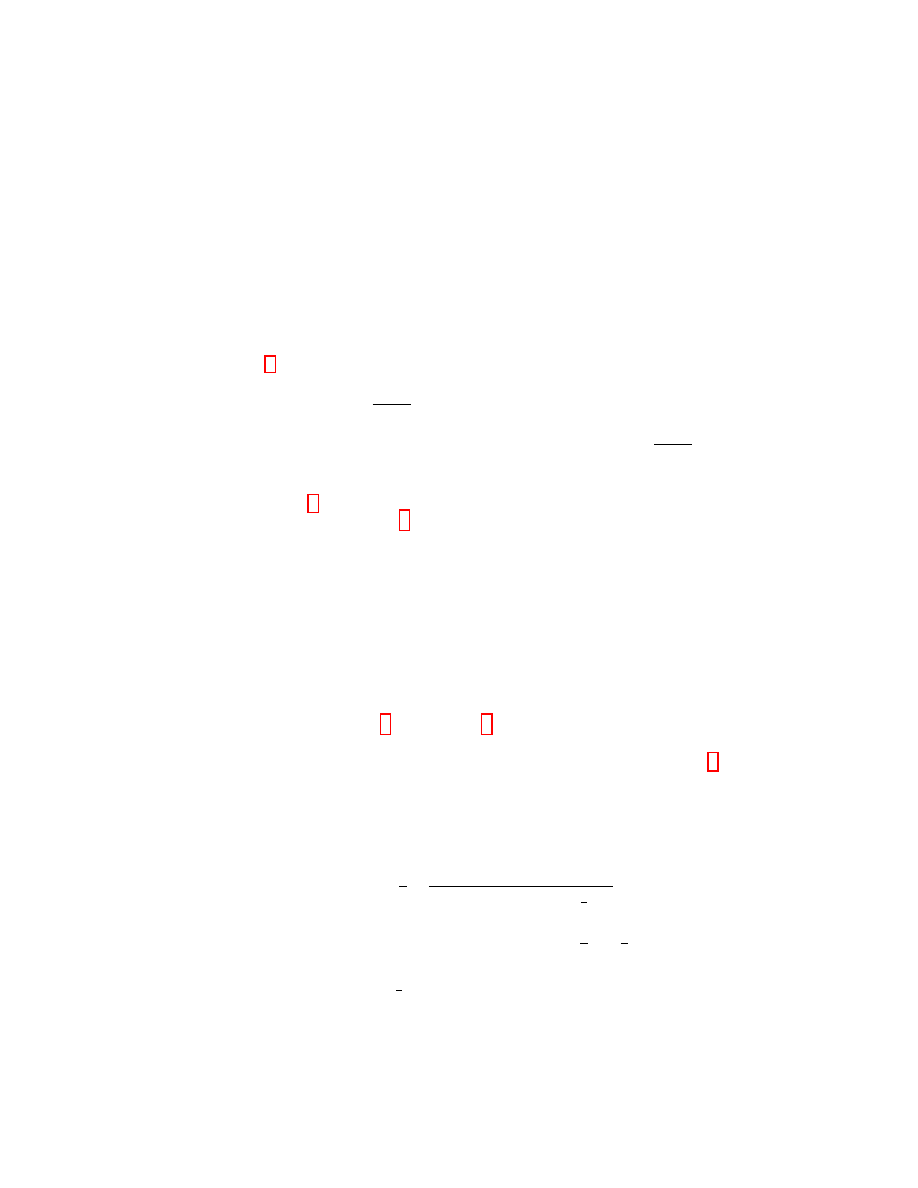
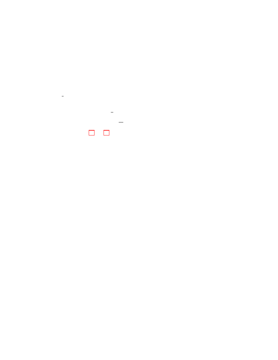
Armed with these settings, Figure 4(a) and Figure 4(b) show the maximum

resistance to mafia fraud for the three protocols considering the cases (a) and
(b) respectively.

Figure 4(a) shows the mafia fraud resistance of the three protocols when

p

f

= p

b

. As expected, the higher the noise the lower the provided security of

the three protocols. In this scenario, however, our protocol is clearly the best
even though KA2 achieves the highest resistance when no noise is considered
(p

f

= p

b

= 0).

A different scenario (p

f

+ p

b

= 0.05) is shown by Figure 4(b). There, the

security of HK improves with p

f

, while KA2 and our protocol are clearly sensitive

to the increase of p

f

. This is an inherent problem of both protocols since a noise

in the forward channel could cause a “desynchronization” between the prover and
the verifier. Nevertheless, thanks to the noise resilience mechanism proposed in
Section 7.2, our protocol deals with noise much better than KA2 and, in general,
performs better than both HK and KA2.

9

Conclusions

A new lightweight distance-bounding protocol has been introduced in this ar-
ticle. The protocol simultaneously deals with both mafia and distance frauds,
without sacrificing memory or requiring additional computation. The analytical
expressions and experimental results show that the new protocol outperforms the
previous ones. This benefit is obtained through the use of dependent rounds in
the fast phase. The protocol also goes a step further by dealing with the inherent
background noise on the communication channels. This is a serious advantage
compared to the other existing protocols.

Appendix

Theorem 6. Let x be the maximum number of errors allowed by the verifier in
the HK protocol. The false rejection ratio HK

availability

p

f

,p

b

,n

(x) can be computed as

follows:

HK

availability

p

f

,p

b

,n

(x) =

n

X

i=n−x

n

i

×

1 −

p

f

2

− p

b

+ p

f

p

b

i

p

f

2

+ p

b

− p

f

p

b

n−i

.

Proof. Let W be the event that a legitimate prover’s bit-answer is correct for
the verifier. The false rejection ratio HK

availability

p

f

,p

b

,n

(x) can be expressed in terms

20

1e-014

1e-012

1e-010

1e-008

1e-006

0.0001

0.01

1

0

0.01

0.02

0.03

0.04

0.05

Mafia Fraud

p

f

HK

KA2

Our proposal

(a) p

f

= p

b

1e-006

1e-005

0.0001

0.001

0.01

0.1

1

0

0.01

0.02

0.03

0.04

0.05

Mafia Fraud

p

f

HK

KA2

Our proposal

(b) p

f

+ p

b

= 0.05

Fig. 4. The maximum resistance to mafia fraud of HK, KA2, and our proposal, con-
sidering 48 rounds, a false rejection ratio lower than 5%, and different values p

f

and

p

b

: in Figure 4(a) p

f

= p

b

∈ {0, 0.005, ..., 0.045, 0.05}, and in Figure 4(b) p

f

+ p

b

= 0.05

where p

f

∈ {0, 0.005, ..., 0.045, 0.05}.

21

of W as follows:

HK

availability

p

f

,p

b

,n

(x) =

n

X

i=n−x

n

i

Pr(W )

i

(1 − Pr(W ))

n−i

.

(17)

It should be noted that if a noise occurs on the forward channel then Pr(W ) =

1
2

, which happens with probability p

f

(1 − p

b

) + p

f

p

b

. Thus:

Pr(W ) =

1

2

(p

f

(1 − p

b

) + p

f

p

b

) + (1 − p

f

)(1 − p

b

)

= 1 −

p

f

2

− p

b

+ p

f

p

b

.

(18)

Equations 17 and 18 yield the expected result.

References

1. G. Avoine, M. A. Bing¨

ol, S. Karda¸s, C. Lauradoux, and B. Martin. A Framework

for Analyzing RFID Distance Bounding Protocols. Journal of Computer Security,
19(2):289–317, March 2011.

2. G. Avoine and A. Tchamkerten. An efficient distance bounding RFID authen-

tication protocol: balancing false-acceptance rate and memory requirement. In
Information Security Conference – ISC’09, volume 5735, pp. 250–261, 2009.

3. S. Bengio, G. Brassard, Y. Desmedt, C. Goutier, and J.-J. Quisquater. Secure

implementation of identification systems.

Journal of Cryptology, 4(3):175–183,

1991.

4. S. Brands and D. Chaum. Distance-bounding protocols. In Workshop on the the-

ory and app.lication of cryptographic techniques on Advances in cryptology, EU-
ROCRYPT ’93, pp. 344–359.

5. J. H. Conway. On Numbers and Games. AK Peters, Ltd., 2nd edition, Dec. 2000.
6. Y. Desmedt, C. Goutier, and S. Bengio. Special uses and abuses of the Fiat-Shamir

passport protocol. In Theory and App.lications of Cryptographic Techniques on
Advances in Cryptology, CRYPTO ’87, pp. 21–39.

7. S. Drimer and S. J. Murdoch. Keep your enemies close: distance bounding against

smartcard relay attacks. In USENIX Security Symposium on USENIX Security
Symposium, pp. 1–16, 2007.

8. A. Fiat and A. Shamir. How to prove yourself: Practical solutions to identification

and signature problems. In Advances in Cryptology – CRYPTO’86, volume 263,
pp. 186–194.

9. R. Trujillo-Rasua, Complexity of distance fraud attacks in graph-based distance

bounding, 10th International Conference on Mobile and Ubiquitous Systems: Com-
puting, Networking and Services, MobiQuitous’13.

10. L. Francis, G. Hancke, K. Mayes, and K. Markantonakis. Practical NFC peer-to-

peer relay attack using mobile phones. In Radio frequency identification: security
and privacy issues, RFIDSec’10, pp. 35–49.

11. G. P. Hancke and M. G. Kuhn. An RFID distance bounding protocol. In Security

and Privacy for Emerging Areas in Communications Networks, pp. 67–73, 2005.

22

12. G. P. Hancke and M. G. Kuhn. Attacks on time-of-flight distance bounding chan-

nels. In Proceedings of the first ACM conference on Wireless network security,
WiSec ’08, pp. 194–202.

13. C. H. Kim and G. Avoine. RFID Distance Bounding Protocols with Mixed Chal-

lenges. IEEE Transactions on Wireless Communications, 10(5):1618–1626, 2011.

14. Y. Oren and A. Wool. Relay attacks on RFID-based electronic voting systems.

Cryptology ePrint Archive, Report 2009/422, 2009.

15. D. Singel´

ee and B. Preneel. Distance bounding in noisy environments. In Security

and privacy in ad-hoc and sensor networks, ESAS’07, pp. 101–115.

16. R. Trujillo-Rasua, B. Martin, and G. Avoine. The poulidor distance-bounding pro-

tocol. In Radio frequency identification: security and privacy issues, RFIDSec’10,
pages 239–257.

17. D. Singel´

ee, B. Preneel, Distance bounding in noisy environments, in: Proceedings

of the 4th European conference on Security and privacy in ad-hoc and sensor
networks, ESAS’07, pp. 101–115.

18. R. Trujillo-Rasua, B. Martin and G. Avoine. Distance-bounding facing both mafia

and distance frauds. IEEE Transactions on Wireless Communications, 2014.

23