
Analytic Semigroups and Reaction-Diffusion
Problems
Internet Seminar 2004–2005
Luca Lorenzi, Alessandra Lunardi, Giorgio Metafune, Diego Pallara
February 16, 2005


Contents
1
Sectorial operators and analytic semigroups
7
1.1
Introduction . . . . . . . . . . . . . . . . . . . . . . . . . . . . . . . . . . . .
7
1.2
Bounded operators . . . . . . . . . . . . . . . . . . . . . . . . . . . . . . . .
7
1.3
Sectorial operators . . . . . . . . . . . . . . . . . . . . . . . . . . . . . . . .
10
2
Examples of sectorial operators
23
2.1
The operator Au = u
00
. . . . . . . . . . . . . . . . . . . . . . . . . . . . . .
24
2.1.1
The second order derivative in the real line . . . . . . . . . . . . . .
24
2.1.2
The operator Au = u
00
in a bounded interval, with Dirichlet bound-
ary conditions . . . . . . . . . . . . . . . . . . . . . . . . . . . . . . .
25
2.2
Some abstract examples . . . . . . . . . . . . . . . . . . . . . . . . . . . . .
28
2.3
The Laplacian in R
N
. . . . . . . . . . . . . . . . . . . . . . . . . . . . . . .
30
2.4
The Dirichlet Laplacian in a bounded open set . . . . . . . . . . . . . . . .
35
2.5
More general operators . . . . . . . . . . . . . . . . . . . . . . . . . . . . . .
37
3
Intermediate spaces
41
3.1
The interpolation spaces D
A
(α, ∞) . . . . . . . . . . . . . . . . . . . . . . .
41
3.2
Spaces of class J
α
. . . . . . . . . . . . . . . . . . . . . . . . . . . . . . . . .
48
4
Non homogeneous problems
51
4.1
Strict, classical, and mild solutions . . . . . . . . . . . . . . . . . . . . . . .
51
5
Asymptotic behavior in linear problems
63
5.1
Behavior of e
tA
. . . . . . . . . . . . . . . . . . . . . . . . . . . . . . . . . .
63
5.2
Behavior of e
tA
for a hyperbolic A . . . . . . . . . . . . . . . . . . . . . . .
64
5.3
Bounded solutions of nonhomogeneous problems in unbounded intervals . .
70
5.4
Solutions with exponential growth and exponential decay
. . . . . . . . . .
73
6
Nonlinear problems
77
6.1
Nonlinearities defined in X
. . . . . . . . . . . . . . . . . . . . . . . . . . .
77
6.1.1
Local existence, uniqueness, regularity . . . . . . . . . . . . . . . . .
77
6.1.2
The maximally defined solution . . . . . . . . . . . . . . . . . . . . .
79
6.2
Reaction–diffusion equations and systems . . . . . . . . . . . . . . . . . . .
82
6.2.1
The maximum principle . . . . . . . . . . . . . . . . . . . . . . . . .
84
6.3
Nonlinearities defined in intermediate spaces . . . . . . . . . . . . . . . . . .
90
6.3.1
Local existence, uniqueness, regularity . . . . . . . . . . . . . . . . .
91
6.3.2
Second order PDE’s . . . . . . . . . . . . . . . . . . . . . . . . . . .
95
6.3.3
The Cahn-Hilliard equation . . . . . . . . . . . . . . . . . . . . . . .
97
3

4
Contents
6.3.4
The Kuramoto-Sivashinsky equation . . . . . . . . . . . . . . . . . .
99
7
Behavior near stationary solutions
101
7.1
The principle of linearized stability . . . . . . . . . . . . . . . . . . . . . . . 101
7.1.1
Linearized stability . . . . . . . . . . . . . . . . . . . . . . . . . . . . 102
7.1.2
Linearized instability . . . . . . . . . . . . . . . . . . . . . . . . . . . 104
7.2
A Cauchy-Dirichlet problem . . . . . . . . . . . . . . . . . . . . . . . . . . . 106
A Linear operators and vector-valued calculus
A1
B Basic Spectral Theory
B1
Bibliography
Nomenclature
iii
Index
iii

Introduction
These lectures deal with the functional analytical approach to linear and nonlinear parabolic
problems.
The simplest significant example is the heat equation, either linear
u
t
(t, x) = u
xx
(t, x) + f (t, x),
0 < t ≤ T,
0 ≤ x ≤ 1,
u(t, 0) = u(t, 1) = 0,
0 ≤ t ≤ T,
u(0, x) = u
0
(x),
0 ≤ x ≤ 1,
(1)
or nonlinear,
u
t
(t, x) = u
xx
(t, x) + f (u(t, x)),
t > 0,
0 ≤ x ≤ 1,
u(t, 0) = u(t, 1) = 0,
t ≥ 0,
u(0, x) = u
0
(x),
0 ≤ x ≤ 1.
(2)
In both cases, u is the unknown, and f , u
0
are given. We will write problems (1), (2) as
evolution equations in suitable Banach spaces. To be definite, let us consider problem (1),
and let us set
u(t, ·) = U (t), f (t, ·) = F (t), 0 ≤ t ≤ T,
so that for every t ∈ [0, T ], U (t) and F (t) are functions, belonging to a suitable Banach
space X. The choice of X depends on the type of the results expected, or else on the
regularity properties of the data. For instance, if f and u
0
are continuous functions the
most natural choice is X = C([0, 1]); if f ∈ L
p
((0, T ) × (0, 1)) and u
0
∈ L
p
(0, 1), p ≥ 1,
the natural choice is X = L
p
(0, 1), and so on.
Next, we write (1) as an evolution equation in X,
(
U
0
(t) = AU (t) + F (t),
0 < t ≤ T,
U (0) = u
0
,
(3)
where A is the realization of the second order derivative with Dirichlet boundary condition
in X (that is, we consider functions that vanish at x = 0 and at x = 1). For instance, if
X = C([0, 1]) then
D(A) = {ϕ ∈ C
2
([0, 1]) : ϕ(0) = ϕ(1) = 0}, (Aϕ)(x) = ϕ
00
(x).
Problem (3) is a Cauchy problem for a linear differential equation in the space X =
C([0, 1]). However, the theory of ordinary differential equations is not easily extendable
5

6
Contents
to this type of problems, because the linear operator A is defined on a proper subspace of
X, and it is not continuous.
What we use is an important spectral property of A: the resolvent set of A contains a
sector S = {λ ∈ C : λ 6= 0, |arg λ| < θ}, with θ > π/2 (precisely, it consists of a sequence
of negative eigenvalues), and moreover
k(λI − A)
−1
k
L(X)
≤
M
|λ|
, λ ∈ S.
(4)
This property will allow us to define the solution of the homogeneous problem (i.e., when
F ≡ 0), that will be called e
tA
u
0
. We shall see that for each t ≥ 0 the linear operator
u
0
7→ e
tA
u
0
is bounded. The family of operators {e
tA
: t ≥ 0} is said to be an analytic
semigroup: semigroup, because it satisfies
e
(t+s)A
= e
tA
e
sA
, t, s ≥ 0, e
0A
= I,
analytic, because the function (0, +∞) 7→ L(X), t 7→ e
tA
is analytic.
Then we shall see that the solution of (3) is given by the variation of constants formula
U (t) = e
tA
u
0
+
Z
t
0
e
(t−s)A
F (s)ds, 0 ≤ t ≤ T,
that will let us study several properties of the solution to (3) and of u, recalling that
U (t) = u(t, ·).
We shall be able to study the asymptotic behavior of U as t → +∞, in the case that
F is defined in [0, +∞). As in the case of ordinary differential equations, the asymptotic
behavior depends heavily on the spectral properties of A.
Also the nonlinear problem (2) will be written as an abstract Cauchy problem,
(
U
0
(t) = AU (t) + F (U (t)), t ≥ 0,
U (0) = u
0
,
(5)
where F : X → X is the composition operator, or Nemitzky operator, F (v) = f (v(·)).
After stating local existence and uniqueness results, we shall see some criteria for existence
in the large. As in the case of ordinary differential equations, in general the solution is
defined only in a small time interval [0, δ]. The problem of existence in the large is of
particular interest in equations coming from mathematical models in physics, biology,
chemistry, etc., where existence in the large is expected. Some sufficient conditions for
existence in the large will be given.
Then we shall study the stability of the (possible) stationary solutions, that is all
the u ∈ D(A) such that Au + F (u) = 0. We shall see that under suitable assumptions
the Principle of Linearized Stability holds. Roughly speaking, u has the same stability
properties of the null solution of the linearized problem
V
0
(t) = AV (t) + F
0
(u)V (t).
A similar study will be made in the case that F is not defined in the whole space X, but
only in an intermediate space between X and D(A). For instance, in several mathematical
models the nonlinearity f (u(t, x)) in problem 2 is replaced by f (u(t, x), u
x
(t, x)). Choosing
again X = C([0, 1]), the composition operator v 7→ F (v) = f (v(·), v
0
(·)) is well defined in
C
1
([0, 1]).

Chapter 1
Sectorial operators and analytic
semigroups
1.1
Introduction
The main topic of our first lectures is the Cauchy problem in a general Banach space X,
(
u
0
(t) = Au(t), t > 0,
u(0) = x,
(1.1)
where A : D(A) → X is a linear operator and x ∈ X. Of course, the construction and the
properties of the solution depends upon the class of operators that is considered. The most
elementary case, which we assume to be known to the reader, is that of a finite dimensional
X and a matrix A. The case of a bounded operator A in general Banach space X can be
treated essentially in the same way, and we are going to discuss it briefly in Section 1.2.
We shall present two formulae for the solution, a power series expansion and an integral
formula with a complex contour integral. While the first one cannot be generalized to
the case of an unbounded A, the contour integral admits a generalization to the sectorial
operators. This class of operators is discussed in Section 1.3. If A is sectorial, then the
solution map x 7→ u(t) of (1.1) is given by an analytic semigroup. Sectorial operators and
analytic semigroups are basic tools in the theory of abstract parabolic problems, and of
partial differential equations and systems of parabolic type.
1.2
Bounded operators
Let A ∈ L(X).
First, we give the solution of (1.1) as the sum of a power series of
exponential type.
Proposition 1.2.1 Let A ∈ L(X). Then, the series
+∞
X
k=0
t
k
A
k
k!
,
t ∈ Re,
(1.2)
converges in L(X) uniformly on bounded subsets of Re. Setting u(t) :=
P
+∞
k=0
t
k
A
k
x/k!,
the restriction of u to [0, +∞) is the unique solution of the Cauchy problem (1.1).
7

8
Chapter 1
Proof. Existence. Using Theorem A.3 as in the finite dimensional case, it is easily checked
that solving (1.1) is equivalent to finding a continuous function v : [0, +∞) → X which
satisfies
v(t) = x +
Z
t
0
Av(s)ds, t ≥ 0.
(1.3)
In order to show that u solves (1.3), let us fix an interval [0, T ] and define
u
0
(t) = x, u
n+1
(t) = x +
Z
t
0
Au
n
(s)ds, n ∈ N.
(1.4)
We have
u
n
(t) =
n
X
k=0
t
k
A
k
k!
x, n ∈ N.
Since
t
k
A
k
k!
≤
T
k
kAk
k
k!
, t ∈ [0, T ],
the series
P
+∞
k=0
t
k
A
k
/k! converges in L(X), uniformly with respect to t in [0, T ]. Moreover,
the sequence {u
n
(t)}
n∈N
converges to u(t) uniformly for t in [0, T ]. Letting n → ∞ in
(1.4), we conclude that u is a solution of (1.3).
Uniqueness. If u, v are two solutions of (1.3) in [0, T ], we have by Proposition A.2(c)
ku(t) − v(t)k ≤ kAk
Z
t
0
ku(s) − v(s)kds
and from Gronwall’s lemma (see Exercise 3 in §1.2.4 below), the equality u = v follows at
once.
As in the finite dimensional setting, we define
e
tA
=
+∞
X
k=0
t
k
A
k
k!
, t ∈ R,
(1.5)
In the proof of Proposition 1.2.1 we have seen that for every bounded operator A the above
series converges in L(X) for each t ∈ R. If A is unbounded, the domain of A
k
may become
smaller and smaller as k increases, and even for x ∈
T
k∈N
D(A
k
) it is not obvious that
the series
P
+∞
k=0
t
k
A
k
x/k! converges. For instance, take X = C([0, 1]), D(A) = C
1
([0, 1]),
Af = f
0
.
Therefore, we have to look for another representation of the solution to (1.1) if we
want to extend it to the unbounded case. As a matter of fact, it is given in the following
proposition.
Proposition 1.2.2 Let A ∈ L(X) and let γ ⊂ C be any circle with centre 0 and radius
r > kAk. Then
e
tA
=
1
2πi
Z
γ
e
tλ
R(λ, A) dλ,
t ∈ R.
(1.6)
Proof. From (1.5) and the power series expansion
R(λ, A) =
+∞
X
k=0
A
k
λ
k+1
,
|λ| > kAk,

1.2. Bounded operators
9
(see (B.10)), we have
1
2πi
Z
γ
e
tλ
R(λ, A) dλ
=
1
2πi
+∞
X
n=0
t
n
n!
Z
γ
λ
n
R(λ, A) dλ
=
1
2πi
+∞
X
n=0
t
n
n!
Z
γ
λ
n
+∞
X
k=0
A
k
λ
k+1
dλ
=
1
2πi
+∞
X
n=0
t
n
n!
+∞
X
k=0
A
k
Z
γ
λ
n−k−1
dλ = e
tA
,
as the integrals in the last series equal 2πi if n = k, 0 otherwise. Note that the exchange
of integration and summation is justified by the uniform convergence.
Let us see how it is possible to generalize to the infinite dimensional setting the variation
of constants formula, that gives the solution of the non-homogeneous Cauchy problem
(
u
0
(t) = Au(t) + f (t), 0 ≤ t ≤ T,
u(0) = x,
(1.7)
where A ∈ L(X), x ∈ X, f ∈ C([0, T ]; X) and T > 0.
Proposition 1.2.3 The Cauchy problem (1.7) has a unique solution in [0, T ], given by
u(t) = e
tA
x +
Z
t
0
e
(t−s)A
f (s)ds,
t ∈ [0, T ].
(1.8)
Proof. It can be directly checked that u is a solution. Concerning uniqueness, let u
1
, u
2
be two solutions; then, v = u
1
− u
2
satisfies v
0
(t) = Av(t) for 0 ≤ t ≤ T , v(0) = 0. By
Proposition 1.2.1, we conclude that v ≡ 0.
Exercises 1.2.4
1. Prove that e
tA
e
sA
= e
(t+s)A
for any t, s ∈ R and any A ∈ L(X).
2. Prove that if the operators A, B ∈ L(X) commute (i.e. AB = BA), then e
tA
e
tB
=
e
t(A+B)
for any t ∈ R.
3. Prove the following form of Gronwall’s lemma:
Let u, v : [0, +∞) → [0, +∞) be continuous functions, and assume that
u(t) ≤ α +
Z
t
0
u(s)v(s)ds
for some α ≥ 0. Then, u(t) ≤ α exp{
R
t
0
v(s)ds}, for any t ≥ 0.
4. Check that the function u defined in (1.8) is a solution of problem (1.7).

10
Chapter 1
1.3
Sectorial operators
Definition 1.3.1 We say that a linear operator A : D(A) ⊂ X → X is sectorial if there
are constants ω ∈ R, θ ∈ (π/2, π), M > 0 such that
(i)
ρ(A) ⊃ S
θ,ω
:= {λ ∈ C : λ 6= ω, | arg(λ − ω)| < θ},
(ii)
kR(λ, A)k
L(X)
≤
M
|λ − ω|
,
λ ∈ S
θ,ω
.
(1.9)
Note that every sectorial operator is closed, because its resolvent set is not empty.
For every t > 0, the conditions (1.9) allow us to define a bounded linear operator e
tA
on X, through an integral formula that generalizes (1.6). For r > 0, η ∈ (π/2, θ), let γ
r,η
be the curve
{λ ∈ C : | arg λ| = η, |λ| ≥ r} ∪ {λ ∈ C : | arg λ| ≤ η, |λ| = r},
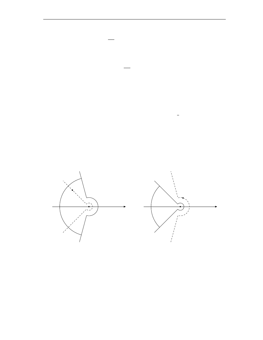
oriented counterclockwise, as in Figure 1.
η
ω
γ
r,η
+ ω
ω + r
σ(A)
Figure 1.1: the curve γ
r,η
.
For each t > 0 set
e
tA
=
1
2πi
Z
γ
r,η
+ω
e
tλ
R(λ, A) dλ, t > 0.
(1.10)
Using the obvious parametrization of γ
r,η
we get
e
tA
=
e
ωt
2πi
−
Z
+∞
r
e
(ρ cos η−iρ sin η)t
R(ω + ρe
−iη
, A)e
−iη
dρ
+
Z
η
−η
e
(r cos α+ir sin α)t
R(ω + re
iα
, A)ire
iα
dα
+
Z
+∞
r
e
(ρ cos η+iρ sin η)t
R(ω + ρe
iη
, A)e
iη
dρ
,
(1.11)
for every t > 0 and for every r > 0, η ∈ (π/2, θ).

1.3. Sectorial operators
11
Lemma 1.3.2 If A is a sectorial operator, the integral in (1.10) is well defined, and it is
independent of r > 0 and η ∈ (π/2, θ).
Proof. First of all, notice that for each t > 0 the mapping λ 7→ e
tλ
R(λ, A) is a L(X)-
valued holomorphic function in the sector S
θ,ω
(see Proposition B.4). Moreover, for any
λ = ω + re
iθ
, the estimate
ke
tλ
R(λ, A)k
L(X)
≤ exp(ωt) exp(tr cos η)
M
r
(1.12)
holds for each λ in the two half-lines, and this easily implies that the improper integral is
convergent. Now take any r
0
> 0, η
0
∈ (π/2, θ) and consider the integral on γ
r
0
,η
0
+ ω. Let
D be the region lying between the curves γ
r,η
+ ω and γ
r
0
,η
0
+ ω and for every n ∈ N set
D
n
= D ∩ {|z − ω| ≤ n}, as in Figure 1.2. By Cauchy integral theorem A.9 we have
Z
∂D
n
e
tλ
R(λ, A) dλ = 0.
By estimate (1.12), the integrals on the two arcs contained in {|z − ω| = n} tend to 0 as
n tends to +∞, so that
Z
γ
r,η
+ω
e
tλ
R(λ, A) dλ =
Z
γ
r0,η0
+ω
e
tλ
R(λ, A) dλ
and the proof is complete.
ω
n
γ
r,η
+ ω
γ
r
0
,η
0
+ ω
D
n
Figure 1.2: the region D
n
.
Let us also set
e
0A
x = x, x ∈ X.
(1.13)
In the following theorem we summarize the main properties of e
tA
for t > 0.

12
Chapter 1
Theorem 1.3.3 Let A be a sectorial operator and let e
tA
be given by (1.10). Then, the
following statements hold.
(i) e
tA
x ∈ D(A
k
) for all t > 0, x ∈ X, k ∈ N. If x ∈ D(A
k
), then
A
k
e
tA
x = e
tA
A
k
x, t ≥ 0.
(ii) e
tA
e
sA
= e
(t+s)A
for any t, s ≥ 0.
(iii) There are constants M
0
, M
1
, M
2
, . . ., such that
(a)
ke
tA
k
L(X)
≤ M
0
e
ωt
, t > 0,
(b)
kt
k
(A − ωI)
k
e
tA
k
L(X)
≤ M
k
e
ωt
, t > 0,
(1.14)
where ω is the number in (1.9). In particular, from (1.14)(b) it follows that for every
ε > 0 and k ∈ N there is C
k,ε
> 0 such that
kt
k
A
k
e
tA
k
L(X)
≤ C
k,ε
e
(ω+ε)t
, t > 0.
(1.15)
(iv) The function t 7→ e
tA
belongs to C
∞
((0, +∞); L(X)), and the equality
d
k
dt
k
e
tA
= A
k
e
tA
, t > 0,
(1.16)
holds for every k ∈ N. Moreover, it has an analytic continuation e
zA
to the sector
S
θ−π/2,0
, and, for z = ρe
iα
∈ S
θ−π/2,0
, θ
0
∈ (π/2, θ − α), the equality
e
zA
=
1
2πi
Z
γ
r,θ0
+ω
e
λz
R(λ, A)dλ
holds.
Proof. Replacing A by A − ωI if necessary, we may suppose ω = 0. See Exercise 1, §1.3.5.
Proof of (i). First, let k = 1. Recalling that A is a closed operator and using Lemma A.4
with f (t) = e
λt
R(λ, A), we deduce that e
tA
x belongs to D(A) for every x ∈ X, and that
Ae
tA
x =
1
2πi
Z
γ
r,η
e
tλ
AR(λ, A)x dλ =
1
2πi
Z
γ
r,η
λe
tλ
R(λ, A)x dλ,
(1.17)
because AR(λ, A) = λR(λ, A) − I, for every λ ∈ ρ(A), and
R
γ
r,η
e
tλ
dλ = 0. Moreover, if
x ∈ D(A), the equality Ae
tA
x = e
tA
Ax follows since AR(λ, A)x = R(λ, A)Ax. Iterating
this argument, we obtain that e
tA
x belongs to D(A
k
) for every k ∈ N; moreover
A
k
e
tA
=
1
2πi
Z
γ
r,η
λ
k
e
tλ
R(λ, A)dλ,
and (i) can be easily proved by recurrence.
Proof of (ii). Since
e
tA
e
sA
=
1
2πi
2
Z
γ
r,η
e
λt
R(λ, A)dλ
Z
γ
2r,η0
e
µs
R(µ, A)dµ,

1.3. Sectorial operators
13
with η
0
∈ (
π
2
, η), using the resolvent identity it follows that
e
tA
e
sA
=
1
2πi
2
Z
γ
r,η
Z
γ
2r,η0
e
λt+µs
R(λ, A) − R(µ, A)
µ − λ
dλdµ
=
1
2πi
2
Z
γ
r,η
e
λt
R(λ, A)dλ
Z
γ
2r,η0
e
µs
dµ
µ − λ
−
1
2πi
2
Z
γ
2r,η0
e
µs
R(µ, A)dµ
Z
γ
r,η
e
λt
dλ
µ − λ
= e
(t+s)A
,
where we have used the equalities
Z
γ
2r,η0
e
µs
dµ
µ − λ
= 2π ie
sλ
,
λ ∈ γ
r,η
,
Z
γ
r,η
e
λt
dλ
µ − λ
= 0,
µ ∈ γ
2r,η
0
(1.18)
that can be easily checked (Exercise 2, §1.3.5).
Proof of (iii). Let us point out that if we estimate ke
tA
k integrating ke
λt
R(λ, A)k over γ
r,η
we get a singularity near t = 0, because the norm of the integrand behaves like M/|λ| for
|λ| small. We have to be more careful. Setting λt = ξ in (1.10) and using Lemma 1.3.2,
we get
e
tA
=
1
2πi
Z
γ
rt,η
e
ξ
R
ξ
t
, A
dξ
t
=
1
2πi
Z
γ
r,η
e
ξ
R
ξ
t
, A
dξ
t
=
1
2πi
Z
+∞
r
e
ρe
iη
R
ρe
iη
t
, A
e
iη
t
dρ −
Z
+∞
r
e
ρe
−iη
R
ρe
−iη
t
, A
e
−iη
t
dρ
+
Z
η
−η
e
re
iα
R
re
iα
t
, A
ire
iα
dα
t
.
It follows that
ke
tA
k ≤
1
π
Z
+∞
r
M e
ρ cos η
dρ
ρ
+
1
2
Z
η
−η
M e
r cos α
dα
.
The estimate of kAe
tA
k is easier, and we do not need the above procedure. Recalling that
kAR(λ, A)k ≤ M + 1 for each λ ∈ γ
r,η
and using (1.11) we get
kAe
tA
k ≤
M + 1
π
Z
+∞
r
e
ρt cos η
dρ +
(M + 1)r
2π
Z
η
−η
e
rt cos α
dα,
so that, letting r → 0,
kAe
tA
k ≤
M + 1
π| cos η|t
:=
N
t
, t > 0.
From the equality Ae
tA
x = e
tA
Ax, which is true for each x ∈ D(A), it follows that
A
k
e
tA
= (Ae
t
k
A
)
k
for all k ∈ N, so that
kA
k
e
tA
k
L(X)
≤ (N kt
−1
)
k
:= M
k
t
−k
.
Proof of (iv). This follows easily from Exercise A.6 and from (1.17). Indeed,
d
dt
e
tA
=
1
2πi
Z
γ
r,η
λe
λt
R(λ, A)dλ = Ae
tA
,
t > 0.
14
Chapter 1
The equality
d
k
dt
k
e
tA
= A
k
e
tA
,
t > 0
can be proved by the same argument, or by recurrence. Now, let 0 < α < θ − π/2 be
given, and set η = θ − α. The function
z 7→ e
zA
=
1
2πi
Z
γ
r,η
e
zλ
R(λ, A)dλ
is well defined and holomorphic in the sector
S
α
= {z ∈ C : z 6= 0, | arg z| < θ − π/2 − α},
because we can differentiate with respect to z under the integral, again by Exercise A.6.
Indeed, if λ = ξe
iη
and z = ρe
iφ
, then Re(zλ) = ξρ cos(η + φ) ≤ −cξρ for a suitable c > 0.
Since the union of the sectors S
α
, for 0 < α < θ − π/2, is S
θ−
π
2
,0
, (iv) is proved.
Statement (ii) in Theorem 1.3.3 tells us that the family of operators e
tA
satisfies the
semigroup law, an algebraic property which is coherent with the exponential notation.
Statement (iv) tells us that e
·A
is analytically extendable to a sector. Therefore, it is
natural to give the following deefinition.
Definition 1.3.4 Let A be a sectorial operator. The function from [0, +∞) to L(X),
t 7→ e
tA
(see (1.10), (1.13)) is called the analytic semigroup generated by A (in X).
−n
λ
γ
r,η
γ
2r,η
0
µ
γ
r,η
γ
2r,η
0
−n
Figure 1.3: the curves for Exercise 2.
Exercises 1.3.5
1. Let A : D(A) ⊂ X → X be sectorial, let α ∈ C, and set B : D(B) := D(A) → X,
Bx = Ax − αx, C : D(C) = D(A) → X, Cx = αAx. Prove that the operator B is
sectorial, and that e
tB
= e
−αt
e
tA
. Use this result to complete the proof of Theorem
1.3.3 in the case ω 6= 0. For which α is the operator C sectorial?
2. Prove that (1.18) holds, integrating over the curves shown in Figure 1.3.

1.3. Sectorial operators
15
3. Let A : D(A) ⊂ X → X be sectorial and let x ∈ D(A) be an eigenvector of A with
eigenvalue λ.
(a) Prove that R(µ, A)x = (µ − λ)
−1
x for any µ ∈ ρ(A).
(b) Prove that e
tA
x = e
λt
x for any t > 0.
4. Prove that if both A and −A are sectorial operators in X, then A is bounded.
Given x ∈ X, the function t 7→ e
tA
x is analytic for t > 0. Let us consider its behavior
for t close to 0.
Proposition 1.3.6 The following statements hold.
(i) If x ∈ D(A), then lim
t→0
+
e
tA
x = x. Conversely, if y = lim
t→0
+
e
tA
x exists, then
x ∈ D(A) and y = x.
(ii) For every x ∈ X and t ≥ 0, the integral
R
t
0
e
sA
x ds belongs to D(A), and
A
Z
t
0
e
sA
x ds = e
tA
x − x.
(1.19)
If, in addition, the function s 7→ Ae
sA
x is integrable in (0, ε) for some ε > 0, then
e
tA
x − x =
Z
t
0
Ae
sA
x ds, t ≥ 0.
(iii) If x ∈ D(A) and Ax ∈ D(A), then lim
t→0
+
(e
tA
x − x)/t = Ax. Conversely, if
z := lim
t→0
+
(e
tA
x − x)/t exists, then x ∈ D(A) and Ax = z ∈ D(A).
(iv) If x ∈ D(A) and Ax ∈ D(A), then lim
t→0
+
Ae
tA
x = Ax.
Proof. Proof of (i). Notice that we cannot let t → 0
+
in the Definition (1.10) of e
tA
x,
because the estimate kR(λ, A)k ≤ M/|λ − ω| does not suffice to use any convergence
theorem.
But if x ∈ D(A) things are easier: indeed fix ξ, r such that ω < ξ ∈ ρ(A), 0 < r < ξ −ω,
and set y = ξx − Ax, so that x = R(ξ, A)y. We have
e
tA
x
=
e
tA
R(ξ, A)y =
1
2πi
Z
γ
r,η
+ω
e
tλ
R(λ, A)R(ξ, A)y dλ
=
1
2πi
Z
γ
r,η
+ω
e
tλ
R(λ, A)
ξ − λ
y dλ −
1
2πi
Z
γ
r,η
+ω
e
tλ
R(ξ, A)
ξ − λ
y dλ
=
1
2πi
Z
γ
r,η
+ω
e
tλ
R(λ, A)
ξ − λ
y dλ,
because the integral
R
γ
r,η
+ω
e
tλ
R(ξ, A)y/(ξ − λ) dλ vanishes (why?).
Here we may let
t → 0
+
because kR(λ, A)y/(ξ − λ)k ≤ C|λ|
−2
for λ ∈ γ
r,η
+ ω. We get
lim
t→0
+
e
tA
x =
1
2πi
Z
γ
r,η
+ω
R(λ, A)
ξ − λ
y dλ = R(ξ, A)y = x.

16
Chapter 1
The second equality follows using Cauchy’s Theorem with the curve {λ ∈ γ
r,η
+ ω :
|λ − ω| ≤ n} ∪ {|λ − ω| = n, arg(λ − ω) ∈ [−η, η]} and then letting n → +∞. Since D(A)
is dense in D(A) and ke
tA
k is bounded by a constant independent of t for 0 < t < 1, then
lim
t→0
+
e
tA
x = x for all x ∈ D(A), see Lemma A.1.
Conversely, if y = lim
t→0
+
e
tA
x, then y ∈ D(A) because e
tA
x ∈ D(A) for t > 0, and
we have R(ξ, A)y = lim
t→0
+
R(ξ, A)e
tA
x = lim
t→0
+
e
tA
R(ξ, A)x = R(ξ, A)x as R(ξ, A)x ∈
D(A). Therefore, y = x.
Proof of (ii). To prove the first statement, take ξ ∈ ρ(A) and x ∈ X. For every ε ∈ (0, t)
we have
Z
t
ε
e
sA
x ds
=
Z
t
ε
(ξ − A)R(ξ, A)e
sA
x ds
=
ξ
Z
t
ε
R(ξ, A)e
sA
x ds −
Z
t
ε
d
ds
(R(ξ, A)e
sA
x)ds
=
ξR(ξ, A)
Z
t
ε
e
sA
x ds − e
tA
R(ξ, A)x + e
εA
R(ξ, A)x.
Since R(ξ, A)x belongs to D(A), letting ε → 0
+
we get
Z
t
0
e
sA
x ds = ξR(ξ, A)
Z
t
0
e
sA
x ds − R(ξ, A)(e
tA
x − x).
(1.20)
Therefore,
R
t
0
e
sA
xds ∈ D(A), and
(ξI − A)
Z
t
0
e
sA
x ds = ξ
Z
t
0
e
sA
x ds − (e
tA
x − x),
whence the first statement in (ii) follows. If in addition s 7→ kAe
sA
xk belongs to L
1
(0, T ),
we may commute A with the integral by Lemma A.4 and the second statement in (ii) is
proved.
Proof of (iii). If x ∈ D(A) and Ax ∈ D(A), we have
e
tA
x − x
t
=
1
t
A
Z
t
0
e
sA
x ds =
1
t
Z
t
0
e
sA
Ax ds.
Since the function s 7→ e
sA
Ax is continuous on [0, t] by (i), then lim
t→0
+
(e
tA
x − x)/t = Ax
by Theorem A.3.
Conversely, if the limit z := lim
t→0
+
(e
tA
x − x)/t exists, then lim
t→0
+
e
tA
x = x, so that
both x and z belong to D(A). Moreover, for every ξ ∈ ρ(A) we have
R(ξ, A)z = lim
t→0
+
R(ξ, A)
e
tA
x − x
t
,
and from (ii) it follows
R(ξ, A)z = lim
t→0
+
1
t
R(ξ, A)A
Z
t
0
e
sA
x ds = lim
t→0
+
(ξR(ξ, A) − I)
1
t
Z
t
0
e
sA
x ds.
Since x ∈ D(A), the function s 7→ e
sA
x is continuous at s = 0, and then
R(ξ, A)z = ξR(ξ, A)x − x.

1.3. Sectorial operators
17
In particular, x ∈ D(A) and z = ξx − (ξ − A)x = Ax.
Proof of (iv). Statement (iv) is an easy consequence of (i), since Ae
tA
x = e
tA
Ax for
x ∈ D(A).
Formula (1.19) is very important. It is the starting point of several proofs and it will
be used throughout these lectures. Therefore, remind it!
It has several variants and consequences. For instance, if ω < 0 we may let t → +∞
and, using (1.14)(a), we get
R
+∞
0
e
sA
xds ∈ D(A) and
x = −A
Z
+∞
0
e
sA
x ds, x ∈ X.
In general, if Re λ > ω, replacing A by A − λI and using (1.19) and Exercise 1, §1.3.5, we
get
e
−λt
e
tA
x − x = (A − λI)
Z
t
0
e
−λs
e
sA
x ds, x ∈ X,
so that
x = (λI − A)
Z
+∞
0
e
−λs
e
sA
x ds, x ∈ X.
(1.21)
An important representation formula for the resolvent R(λ, A) of A follows.
Proposition 1.3.7 Let A : D(A) ⊂ X → X be a sectorial operator. For every λ ∈ C
with Re λ > ω we have
R(λ, A) =
Z
+∞
0
e
−λt
e
tA
dt.
(1.22)
Proof. The right hand side is well defined as an element of L(X) by estimate (1.14)(a).
The equality follows applying R(λ, A) to both sides of (1.21).
Corollary 1.3.8 For all t ≥ 0 the operator e
tA
is one to one.
Proof. e
0A
= I is obviously one to one. If there are t
0
> 0, x ∈ X such that e
t
0
A
x = 0,
then for t ≥ t
0
, e
tA
x = e
(t−t
0
)A
e
t
0
A
x = 0. Since the function t 7→ e
tA
x is analytic, e
tA
x ≡ 0
in (0, +∞). From Proposition 1.3.7 we get R(λ, A)x = 0 for λ > ω, so that x = 0.
Remark 1.3.9 Formula (1.22) is used to define the Laplace transform of the scalar func-
tion t 7→ e
tA
, if A ∈ C. The classical inversion formula to recover e
tA
from its Laplace
transform is given by a complex integral on a suitable vertical line; in our case the vertical
line has been replaced by a curve joining ∞e
−iη
to ∞e
iη
with η > π/2, in such a way that
the improper integral converges by assumption (1.9).
Of course, the continuity properties of semigroups of linear operators are very impor-
tant in their analysis. The following definition is classical.
Definition 1.3.10 Let (T (t))
t≥0
be a family of bounded operators on X. If T (0) = I,
T (t + s) = T (t)T (s) for all t, s ≥ 0 and the map t 7→ T (t)x is continuous from [0, +∞) to
X then we say that (T (t))
t≥0
is a strongly continuous semigroup.

18
Chapter 1
By Proposition 1.3.6(i) we immediately see that the semigroup {e
tA
}
t≥0
is strongly
continuous in X if and only if D(A) is dense in X.
In any case some weak continuity property of the function t 7→ e
tA
x holds for a general
x ∈ X; for instance we have
lim
t→0
+
R(λ, A)e
tA
x = R(λ, A)x
(1.23)
for every λ ∈ ρ(A). Indeed, R(λ, A)e
tA
x = e
tA
R(λ, A)x for every t > 0, and R(λ, A)x ∈
D(A). In the case when D(A) is not dense in X, a standard way to obtain a strongly
continuous semigroup from a sectorial operator A is to consider the part of A in D(A).
Definition 1.3.11 Let L : D(L) ⊂ X → X be a linear operator, and let Y be a subspace
of X. The part of L in Y is the operator L
0
defined by
D(L
0
) = {x ∈ D(L) ∩ Y : Lx ∈ Y }, L
0
x = Lx.
It is easy to see that the part A
0
of A in D(A) is still sectorial. Since D(A
0
) is dense in
D(A) (because for each x ∈ D(A) we have x = lim
t→0
e
tA
x), then the semigroup generated
by A
0
is strongly continuous in D(A). By (1.10), the semigroup generated by A
0
coincides
of course with the restriction of e
tA
to D(A).
Coming back to the Cauchy problem (1.1), let us notice that Theorem 1.3.3 implies
that the function
u(t) = e
tA
x, t ≥ 0
is analytic with values in D(A) for t > 0, and it is a solution of the differential equation
in (1.1) for t > 0. Moreover, u is continuous also at t = 0 (with values in X) if and only
if x ∈ D(A) and in this case u is a solution of the Cauchy problem (1.1). If x ∈ D(A)
and Ax ∈ D(A), then u is continuously differentiable up to t = 0, and it satisfies the
differential equation also at t = 0, i.e., u
0
(0) = Ax. Uniqueness of the solution to (1.1)
will be proved in Proposition 4.1.2, in a more general context.
Let us give a sufficient condition, seemingly weaker than (1.9), in order that a linear
operator be sectorial. It will be useful to prove that the realizations of some elliptic partial
differential operators are sectorial in the usual function spaces.
Proposition 1.3.12 Let A : D(A) ⊂ X → X be a linear operator such that ρ(A) contains
a halfplane {λ ∈ C : Re λ ≥ ω}, and
kλR(λ, A)k
L(X)
≤ M, Re λ ≥ ω,
(1.24)
with ω ≥ 0, M ≥ 1. Then A is sectorial.
Proof. By Proposition B.3, for every r > 0 the open disks with centre ω ± ir and radius
|ω + ir|/M is contained in ρ(A). Since |ω + ir| ≥ r, the union of such disks and of the
halfplane {Re λ ≥ ω} contains the sector {λ ∈ C : λ 6= ω, | arg(λ − ω)| < π − arctan(M )}
and, hence, it contains S = {λ 6= ω : | arg(λ − ω)| < π − arctan(2M )}. If λ ∈ S and
Re λ < ω, we write λ = ω ± ir − (θr)/(2M ) for some θ ∈ (0, 1). Since by (B.4)
R(λ, A) = R(ω ± ir, A) (I + (λ − ω ∓ ir)R(ω ± ir, A))
−1

1.3. Sectorial operators
19
and k(I + (λ − ω ∓ ir)R(ω ± ir, A))
−1
k ≤ 2, we have
kR(λ, A)k ≤
2M
|ω ± ir|
≤
2M
r
≤
√
4M
2
+ 1
|λ − ω|
.
If λ ∈ S and Re λ ≥ ω, estimate (1.24) yields kR(λ, A)k ≤ M/|λ − ω|, and the statement
follows.
Next, we prove a useful perturbation theorem.
Theorem 1.3.13 Let A : D(A) → X be a sectorial operator, and let B : D(B) → X be a
linear operator such that D(A) ⊂ D(B) and
kBxk ≤ akAxk + bkxk,
x ∈ D(A).
(1.25)
There is δ > 0 such that if a ∈ [0, δ] then A + B : D(A) → X is sectorial.
Proof. Let r > 0 be such that R(λ, A) exists and kλR(λ, A)k ≤ M for Re λ ≥ r. We write
λ − A − B = (I − BR(λ, A))(λ − A) and we observe that
kBR(λ, A)xk ≤ akAR(λ, A)xk + bkR(λ, A)xk ≤
a(M + 1) +
bM
|λ|
kxk ≤
1
2
kxk
if a(M + 1) ≤ 1/4 and bM/|λ| ≤ 1/4. Therefore, if a ≤ δ := (4(M + 1))
−1
and for Re λ
sufficiently large, kBR(λ, A)k ≤ 1/2 and
k(λ − A − B)
−1
k ≤ kR(λ, A)k k(I − BR(λ, A))
−1
k ≤
2M
|λ|
.
The statement now follows from Proposition 1.3.12.
Corollary 1.3.14 If A is sectorial and B : D(B) ⊃ D(A) → X is a linear operator such
that for some θ ∈ (0, 1), C > 0 we have
kBxk ≤ Ckxk
θ
D(A)
kxk
1−θ
X
,
x ∈ D(A),
then A + B : D(A + B) := D(A) → X is sectorial.
Remark 1.3.15 In fact the proof of Theorem 1.3.13 shows that if A : D(A) → X is a
sectorial operator and B : D(B) → X is a linear operator such that D(A) ⊂ D(B) and
lim
Re λ→+∞, λ∈S
θ,ω
kBR(λ, A)k = 0, then A + B : D(A) → X is a sectorial operator.
The next theorem is sometimes useful, because it allows to work in smaller subspaces
of D(A). A subspace D as in the following statement is called a core for the operator A.
Theorem 1.3.16 Let A be a sectorial operator with dense domain. If a subspace D ⊂
D(A) is dense in X and e
tA
(D) ⊂ D for each t > 0, then D is dense in D(A) with respect
to the graph norm.

20
Chapter 1
Proof. Fix x ∈ D(A) and a sequence (x
n
) ⊂ D which converges to x in X. Since D(A) is
dense, then by Proposition 1.3.6(iii)
Ax = lim
t→0
+
e
tA
x − x
t
= lim
t→0
+
A
t
Z
t
0
e
sA
x ds,
and the same formula holds with x
n
in place of x. Therefore it is convenient to set
y
n,t
=
1
t
Z
t
0
e
sA
x
n
ds =
1
t
Z
t
0
e
sA
(x
n
− x) ds +
1
t
Z
t
0
e
sA
x ds.
For each n, the map s 7→ e
sA
x
n
is continuous in D(A) and takes values in D; it follows that
R
t
0
e
sA
x
n
ds, being the limit of the Riemann sums, belongs to the closure of D in D(A),
and then each y
n,t
does. Moreover ky
n,t
− xk tends to 0 as t → 0
+
, n → +∞, and
Ay
n,t
− Ax =
e
tA
(x
n
− x) − (x
n
− x)
t
+
1
t
Z
t
0
e
sA
Ax ds − Ax.
Given ε > 0, fix τ so small that kτ
−1
R
τ
0
e
sA
Ax ds − Axk ≤ ε, and then choose n large,
in such a way that (M
0
e
ωτ
+ 1)kx
n
− xk/τ ≤ ε. For such choices of τ and n we have
kAy
n,τ
− Axk ≤ 2ε, and the statement follows.
Theorem 1.3.16 implies that the operator A is the closure of the restriction of A to D,
i.e. D(A) is the set of all x ∈ X such that there is a sequence (x
n
) ⊂ D with the property
that x
n
→ x and Ax
n
converges as n → +∞; in this case we have Ax = lim
n→+∞
Ax
n
.
Remark 1.3.17 Up to now we have considered complex Banach spaces, and the operators
e
tA
have been defined through integrals over paths in C. But in many applications we
have to work in real Banach spaces.
If X is a real Banach space, and A : D(A) ⊂ X → X is a closed linear operator, it is
however convenient to consider its complex spectrum and resolvent. So we introduce the
complexifications of X and of A, defined by
e
X = {x + iy : x, y ∈ X}; kx + iyk
e
X
=
sup
−π≤θ≤π
kx cos θ + y sin θk
and
D( e
A) = {x + iy : x, y ∈ D(A)},
e
A(x + iy) = Ax + iAy.
With obvious notation, we say that x and y are the real and the imaginary part of x + iy.
Note that the “euclidean norm”
pkxk
2
+ kyk
2
is not a norm, in general. See Exercise 5
in §1.3.18.
If the complexification e
A of A is sectorial, so that the semigroup e
t e
A
is analytic in e
X,
then the restriction of e
t e
A
to X maps X into itself for each t ≥ 0. To prove this statement
it is convenient to replace the path γ
r,η
by the path γ = {λ ∈ C : λ = ω
0
+ ρe
±iθ
, ρ ≥ 0},
with ω
0
> ω, in formula (1.10). For each x ∈ X we get
e
t e
A
x =
1
2πi
Z
+∞
0
e
ω
0
t
e
iθ+ρte
iθ
R(ω
0
+ ρe
iθ
, e
A) − e
−iθ+ρte
−iθ
R(ω
0
+ ρe
−iθ
, e
A)
x dρ, t > 0.
The real part of the function under the integral vanishes (why?), and then e
t e
A
x belongs
to X. So, we have a semigroup of linear operators in X which enjoys all the properties
that we have seen up to now.

1.3. Sectorial operators
21
Exercises 1.3.18
1. Let X
k
, k = 1, . . . , n be Banach spaces, and let A
k
: D(A
k
) → X
k
be sectorial
operators. Set
X =
n
Y
k=1
X
k
, D(A) =
n
Y
k=1
D(A
k
),
and A(x
1
, . . . , x
n
) = (A
1
x
1
, . . . , A
n
x
n
), and show that A is a sectorial operator in
X. X is endowed with the product norm k(x
1
, . . . , x
n
)k =
P
n
k=1
kx
k
k
2
1/2
.
2. (a) Let A, B be sectorial operators in X. Prove that e
tA
e
tB
= e
tB
e
tA
for any t > 0
if and only if e
tA
e
sB
= e
sB
e
tA
for any t, s > 0.
(b) Prove that if A and B are as above, then e
tA
e
sB
= e
sB
e
tA
for any t, s > 0 if and
only if R(λ, A)R(µ, B) = R(µ, B)R(λ, A) for large Re λ and Re µ.
3. Let A : D(A) ⊂ X → X and B : D(B) ⊂ X → X be, respectively, a sectorial
operator and a closed operator such that D(A) ⊂ D(B).
(i) Show that there exist two positive constants a and b such that
kBxk ≤ akAxk + bkxk
for every x ∈ D(A).
[Hint: use the closed graph theorem to show that BR(λ, A) is bounded for any
λ ∈ ρ(A)].
(ii) Prove that if BR(λ
0
, A) = R(λ
0
, A)B in D(B) for some λ
0
∈ ρ(A), then
BR(λ, A) = R(λ, A)B in D(B) for any λ ∈ S
θ,ω
.
[Hint: use Proposition B.3].
(iii) Show that if BR(λ
0
, A) = R(λ
0
, A)B in D(B), then Be
tA
= e
tA
B in D(B) for
every t > 0.
4. Prove Corollary 1.3.14.
5. Let X be a real Banach space. Prove that the function f : X × X → R defined by
f (x, y) =
pkxk
2
+ kyk
2
for any x, y ∈ X, may not satisfy, in general, the homo-
geneity property
f (λ(x, y)) = |λ|f (x, y), λ ∈ C.

22
Chapter 2

Chapter 2
Examples of sectorial operators
In this chapter we show several examples of sectorial operators.
The leading example is the Laplace operator ∆ in one or more variables, i.e., ∆u = u
00
if N = 1 and ∆u =
P
N
i=1
D
ii
u if N > 1. We shall see some realizations of the Laplacian
in different Banach spaces, and with different domains, that turn out to be sectorial
operators.
The Banach spaces taken into consideration are the usual spaces of complex valued
functions defined in R
N
or in an open set Ω of R
N
, that we recall briefly below.
The Lebesgue spaces L
p
(Ω), 1 ≤ p ≤ +∞, are endowed with the norms
kf k
L
p
(Ω)
=
Z
Ω
|f (x)|
p
dx
1/p
, 1 ≤ p < +∞,
kf k
L
∞
(Ω)
= ess sup
x∈Ω
|f (x)|.
When no confusion may arise, we write kf k
p
for kf k
L
p
(Ω)
.
The Sobolev spaces W
k,p
(Ω), where k is any positive integer and 1 ≤ p ≤ +∞, consist
of all the functions f in L
p
(Ω) which admit weak derivatives D
α
f for |α| ≤ k belonging
to L
p
(Ω). They are endowed with the norm
kf k
W
k,p
(Ω)
=
X
|α|≤k
kD
α
f k
p
.
If p = 2, we write H
k
(Ω) for W
k,p
(Ω).
C
b
(Ω) (resp., BU C(Ω)) is the space of all the bounded and continuous (resp., bounded
and uniformly continuous) functions f : Ω → C. They are endowed with the L
∞
norm.
If k ∈ N, C
k
b
(Ω) (resp. BU C
k
(Ω)) is the space of all the functions f in C
b
(Ω) (resp. in
BU C(Ω)) which are k times continuously differentiable in Ω, with all the derivatives up
to the order k in C
b
(Ω) (resp. in BU C(Ω)). They are endowed with the norm
kf k
C
k
b
(Ω)
=
X
|α|≤k
kD
α
f k
∞
.
If Ω is bounded, we drop the subindex b and we write C(Ω), C
k
(Ω).
23

24
Chapter 2. Examples of sectorial operators
2.1
The operator Au = u
00
2.1.1
The second order derivative in the real line
Throughout the section we shall use square roots of complex numbers, defined by
√
λ =
|λ|
1/2
e
iθ/2
if arg λ = θ ∈ (−π, π]. Therefore, Re
√
λ > 0 if λ ∈ C \ (−∞, 0].
Let us define the realizations of the second order derivative in L
p
(R) (1 ≤ p < +∞),
and in C
b
(R), endowed with the maximal domains
D(A
p
) = W
2,p
(R) ⊂ L
p
(R),
A
p
u = u
00
,
1 ≤ p < +∞,
D(A
∞
) = C
2
b
(R),
A
∞
u = u
00
.
Let us determine the spectrum of A
p
and estimate the norm of its resolvent.
Proposition 2.1.1 For all 1 ≤ p ≤ +∞ the spectrum of A
p
is the halfline (−∞, 0]. If
λ = |λ|e
iθ
with |θ| < π then
kR(λ, A)k
L(L
p
(R))
≤
1
|λ| cos(θ/2)
.
Proof. First we show that (−∞, 0] ⊂ σ(A
p
).
Fix λ ≤ 0 and consider the function
u(x) = exp(i
√
−λx) which satisfies u
00
= λu. For p = +∞, u is an eigenfunction of A
∞
with eigenvalue λ. For p < +∞, u does not belong to L
p
(R). To overcome this difficulty,
consider a cut-off function ψ : R → R, supported in [−2, 2] and identically equal to 1 in
[−1, 1] and set ψ
n
(x) = ψ(x/n), for any n ∈ N.
If u
n
= ψ
n
u, then u
n
∈ D(A
p
) and ku
n
k
p
≈ n
1/p
as n → +∞. Moreover, kAu
n
−
λu
n
k
p
≤ Cn
1/p−1
. Setting v
n
= u
n
/ku
n
k
p
, it follows that k(λ − A)v
n
k
p
→ 0 as n → +∞,
and then λ ∈ σ(A). See Exercise B.9.
Now let λ 6∈ (−∞, 0]. If p = +∞, the equation λu − u
00
= 0 has no nonzero bounded
solution, hence λI − A
∞
is one to one. If p < +∞, it is easy to see that all the nonzero
solutions u ∈ W
2,p
loc
(R) to the equation λu − u
00
= 0 belong to C
∞
(R) and they are classical
solutions, but they do not belong to L
p
(R), so that the operator λI − A
p
is one to one.
We recall that W
2,p
loc
(R) denotes the set of all the functions f : R → R which belong to
W
2,p
(I) for any bounded interval I ⊂ R.
Let us show that λI − A
p
is onto. We write
√
λ = µ. If f ∈ C
b
(R) the variation of
constants method gives the (unique) bounded solution to λu − u
00
= f , written as
u(x) =
1
2µ
Z
x
−∞
e
−µ(x−y)
f (y)dy +
Z
+∞
x
e
µ(x−y)
f (y)dy
= (f ? h
µ
)(x),
(2.1)
where h
µ
(x) = e
−µ|x|
/2µ. Since kh
µ
k
L
1
(R)
= (|µ| Re µ)
−1
, we get
kuk
∞
≤ kh
µ
k
L
1
(R)
kf k
∞
=
1
|λ| cos(θ/2)
kf k
∞
,
where θ = arg λ. If |θ| ≤ θ
0
< π we get kuk
∞
≤ (|λ| cos(θ
0
/2))
−1
kf k
∞
, and therefore A
∞
is sectorial, with ω = 0 and any θ ∈ (π/2, π).
If p < +∞ and f ∈ L
p
(R), the natural candidate to be R(λ, A
p
)f is still the function u
defined by (2.1). We have to check that u ∈ D(A
p
) and that (λI − A
p
)u = f . By Young’s
inequality (see e.g. [3, Th. IV.15]), u ∈ L
p
(R) and again
kuk
p
≤ kf k
p
kh
µ
k
1
≤
1
|λ| cos(θ/2)
kf k
p
.

2.1. The operator Au = u
00
25
That u ∈ D(A
p
) may be seen in several ways; all of them need some knowledge of ele-
mentary properties of Sobolev spaces. The following proof relies on the fact that smooth
functions are dense in W
1,p
(R)
(1)
.
Approximate f ∈ L
p
(R) by a sequence (f
n
) ⊂ C
∞
0
(R). The corresponding solutions
u
n
to λu
n
− u
00
n
= f
n
are smooth and they are given by formula (2.1) with f
n
instead of f ,
therefore they converge to u by Young’s inequality. Moreover,
u
0
n
(x) = −
1
2
Z
x
−∞
e
−µ(x−y)
f
n
(y)dy +
1
2
Z
+∞
x
e
µ(x−y)
f
n
(y)dy
converge to the function
g(x) = −
1
2
Z
x
−∞
e
−µ(x−y)
f (y)dy +
1
2
Z
+∞
x
e
µ(x−y)
f (y)dy
again by Young’s inequality. Hence g = u
0
∈ L
p
(R), and u
00
n
= λu
n
− f
n
converge to λu − f ,
hence λu − f = u
00
∈ L
p
(R). Therefore u ∈ W
2,p
(R) and the statement follows.
Note that D(A
∞
) is not dense in C
b
(R), and its closure is BU C(R). Therefore, the
associated semigroup e
tA
∞
is not strongly continuous. But the part of A
∞
in BU C(R),
i.e. the operator
BU C
2
(R) → BU C(R), u 7→ u
00
has dense domain in BU C(R) and it is sectorial, so that the restriction of e
tA
∞
to BU C(R)
is strongly continuous. If p < +∞, D(A
p
) is dense in L
p
(R), and e
tA
p
is strongly continuous
in L
p
(R).
This is one of the few situations in which we have a nice representation formula for
e
tA
p
, for 1 ≤ p ≤ +∞, and precisely
(e
tA
p
f )(x) =
1
(4πt)
1/2
Z
R
e
−
|x−y|2
4t
f (y)dy, t > 0, x ∈ R.
(2.2)
This formula will be discussed in Section 2.3, where we shall use a classical method,
based on the Fourier transform, to obtain it.
In principle, since we have an explicit
representation formula for the resolvent, plugging it in (1.10) we should get (2.2). But the
contour integral obtained in this way is not very easy to work out.
2.1.2
The operator Au = u
00
in a bounded interval, with Dirichlet bound-
ary conditions
Without loss of generality, we fix I = (0, 1), and we consider the realizations of the second
order derivative in L
p
(0, 1), 1 ≤ p < +∞,
D(A
p
) = {u ∈ W
2,p
(0, 1) : u(0) = u(1) = 0} ⊂ L
p
(0, 1), A
p
u = u
00
,
as well as its realization in C([0, 1]),
D(A
∞
) = {u ∈ C
2
([0, 1]) : u(0) = u(1) = 0}, A
∞
u = u
00
.
1
Precisely, a function v ∈ L
p
(R) belongs to W
1,p
(R) iff there is a sequence (v
n
) ⊂ C
∞
(R) with v
n
,
v
0
n
∈ L
p
(R), such that v
n
→ v and v
0
n
→ g in L
p
(R) as n → +∞. In this case, g is the weak derivative of
v. See [3, Chapter 8].

26
Chapter 2. Examples of sectorial operators
We could follow the same approach of Subsection 2.1.1, by computing the resolvent oper-
ator R(λ, A
∞
) for λ /
∈ (−∞, 0] and then showing that the same formula gives R(λ, A
p
).
The formula turns out to be more complicated than before, but it leads to the same final
estimate, see Exercise 3 in §2.1.3. Here we do not write it down explicitly, but we estimate
separately its components, arriving at a less precise estimate for the norm of the resolvent,
with simpler computations.
Proposition 2.1.2 The operators A
p
: D(A
p
) → L
p
(0, 1), 1 ≤ p < +∞ and A
∞
:
D(A
∞
) → C([0, 1]) are sectorial, with ω = 0 and any θ ∈ (π/2, π).
Proof. For λ /
∈ (−∞, 0] set µ =
√
λ, so that Re µ > 0. For every f ∈ X, X = L
p
(0, 1)
or X = C([0, 1]), extend f to a function e
f ∈ L
p
(R) or e
f ∈ C
b
(R), in such a way that
k e
f k = kf k. For instance we may define e
f (x) = 0 for x /
∈ (0, 1) if X = L
p
(0, 1), e
f (x) = f (1)
for x > 1, e
f (x) = f (0) for x < 0 if X = C([0, 1]). Let
e
u be defined by (2.1) with e
f instead
of f . We already know from Proposition 2.1.1 that
e
u
|[0,1]
is a solution of the equation
λu − u
00
= f satisfying kuk
p
≤ kf k
p
/(|λ| cos(θ/2)), where θ = arg λ. However, it does not
necessarily satisfy the boundary conditions. To find a solution that satisfies the boundary
conditions we set
γ
0
=
1
2µ
Z
R
e
−µ|s|
e
f (s) ds =
e
u(0)
and
γ
1
=
1
2µ
Z
R
e
−µ|1−s|
e
f (s) ds =
e
u(1).
All the solutions of the equation λu − u
00
= f belonging to W
2,p
(0, 1) or to C
2
([0, 1]) are
given by
u(x) =
e
u(x) + c
1
u
1
(x) + c
2
u
2
(x),
where u
1
(x) := e
−µx
and u
2
(x) := e
µx
are two independent solutions of the homogeneous
equation λu − u
00
= 0. We determine uniquely c
1
and c
2
imposing u(0) = u(1) = 0 because
the determinant
D(µ) = e
µ
− e
−µ
is nonzero since Re µ > 0. A straightforward computation yields
c
1
=
1
D(µ)
[γ
1
− e
µ
γ
0
] ,
c
2
=
1
D(µ)
−γ
1
+ e
−µ
γ
0
,
so that for 1 ≤ p < +∞
ku
1
k
p
≤
1
(p Re µ)
1/p
;
ku
2
k
p
≤
e
Re µ
(p Re µ)
1/p
;
while ku
1
k
∞
= 1, ku
2
k
∞
= e
Re µ
. For 1 < p < +∞ by the H¨
older inequality we also obtain
|γ
0
| ≤
1
2|µ|(p
0
Re µ)
1/p
0
kf k
p
,
|γ
1
| ≤
1
2|µ|(p
0
Re µ)
1/p
0
kf k
p
and
|γ
j
| ≤
1
2|µ|
kf k
1
,
if f ∈ L
1
(0, 1), j = 0, 1
|γ
j
| ≤
1
|µ| Re µ
kf k
∞
,
if f ∈ C([0, 1]), j = 0, 1.

2.1. The operator Au = u
00
27
Moreover |D(µ)| ≈ e
Re µ
for |µ| → +∞. If λ = |λ|e
iθ
with |θ| ≤ θ
0
< π then Re µ ≥
|µ| cos(θ
0
/2) and we easily get
kc
1
u
1
k
p
≤
C
|λ|
kf k
p
and
kc
2
u
2
k
p
≤
C
|λ|
kf k
p
for a suitable C > 0 and λ as above, |λ| large enough. Finally
kuk
p
≤
C
|λ|
kf k
p
for |λ| large, say |λ| ≥ R, and | arg λ| ≤ θ
0
.
For |λ| ≤ R we may argue as follows: one checks easily that the spectrum of A
p
consists
only of the eigenvalues −n
2
π
2
, n ∈ N. Since λ 7→ R(λ, A
p
) is holomorphic in the resolvent
set, it is continuous, hence it is bounded on the compact set {|λ| ≤ R, | arg λ| ≤ θ
0
} ∪{0}.
Exercises 2.1.3
1. Let A
∞
be the operator defined in Subsection 2.1.1.
(a) Prove that the resolvent R(λ, A
∞
) leaves invariant the subspaces
C
0
(R) := {u ∈ C(R) :
lim
|x|→+∞
u(x) = 0}
and
C
T
(R) := {u ∈ C(R) : u(x) = u(x + T ), x ∈ R},
with T > 0.
(b) Using the previous results show that the operators
A
0
: D(A
0
) := {u ∈ C
2
(R) ∩ C
0
(R) : u
00
∈ C
0
(R)} → C
0
(R), A
0
u = u
00
,
and
A
T
: D(A
T
) := C
2
(R) ∩ C
T
(R) → C
T
(R), A
T
u = u
00
are sectorial in C
0
(R) and in C
T
(R), respectively.
2. (a) Let λ > 0 and set
φ(x) =
Z
+∞
0
1
√
4πt
e
−λt
e
−x
2
/4t
dt.
Prove that φ
00
= λφ and φ(0) = (2
√
πλ)
−1
Γ(1/2) = (2
√
λ)
−1
, φ(x) → 0 as |x| →
+∞, so that φ coincides with the function h
√
λ
in (2.1). (b) Use (a) and Proposition
1.3.7 to prove formula (2.2).
3. Consider again the operator u 7→ u
00
in (0, 1) as in Subsection 2.1.2, with the domains
D(A
p
) defined there, 1 ≤ p ≤ +∞.
Solving explicitly the differential equation
λu − u
00
= f in D(A
p
), show that the eigenvalues are −n
2
π
2
, n ∈ N, and express the
resolvent as an integral operator.

28
Chapter 2. Examples of sectorial operators
4. Consider the operator A
p
u = u
00
in L
p
(0, 1), 1 ≤ p < ∞, with the domain
D(A
p
) = {u ∈ W
2,p
(0, 1) : u
0
(0) = u
0
(1) = 0} ⊂ L
p
(0, 1),
or in C([0, 1]), with the domain
D(A
∞
) = {u ∈ C
2
((0, 1)) ∩ C([0, 1]) : u
0
(0) = u
0
(1) = 0},
corresponding to the Neumann boundary condition.
Use the same argument of
Subsection 2.1.2 to show that A
p
is sectorial.
5. Let A
∞
be the realization of the second order derivative in C([0, 1]) with Dirichlet
boundary condition, as in Subsection 2.1.2. Prove that for each α ∈ (0, 1) the part
of A
∞
in C
α
([0, 1]), i.e. the operator
{u ∈ C
2+α
([0, 1]) : u(0) = u(1) = 0} → C
α
([0, 1]), u 7→ u
00
is not sectorial in C
α
([0, 1]), although the function (0, +∞) → L(C
α
([0, 1])), t 7→
e
tA
∞
|C
α
([0,1])
is analytic.
[Hint: take f ≡ 1, compute explicitly u := R(λ, A
∞
)f for λ > 0, and show that
lim sup
λ→+∞
λ
1+α/2
u(λ
−1/2
) = +∞, so that λ[R(λ, A
∞
)f ]
C
α
is unbounded as λ →
+∞. ]
Taking into account the behavior of R(λ, A)1, deduce that ke
tA
k
L(C
α
([0,1]))
is un-
bounded for t ∈ (0, 1).
2.2
Some abstract examples
The realization of the second order derivative in L
2
(R) is a particular case of the following
general situation. Recall that, if H is a Hilbert space, and A : D(A) ⊂ H → H is a linear
operator with dense domain, the adjoint A
∗
of A is the operator A
∗
: D(A
∗
) ⊂ X → X
defined as follows,
D(A
∗
) = {x ∈ H : ∃y ∈ H such that hAz, xi = hz, yi, ∀z ∈ D(A)},
A
∗
x = y.
The operator A is said to be self-adjoint if D(A) = D(A
∗
) and A = A
∗
. It is said to be
dissipative if
k(λ − A)xk ≥ λkxk,
(2.3)
for all x ∈ D(A) and λ > 0, or equivalently (see Exercises 2.2.4) if RehAx, xi ≤ 0 for every
x ∈ D(A).
The following proposition holds.
Proposition 2.2.1 Let H be a Hilbert space, and let A : D(A) ⊂ H → H be a self-adjoint
dissipative operator. Then A is sectorial, with an arbitrary θ < π and ω = 0.
Proof. Let us first show that σ(A) ⊂ R. Let λ = a + ib ∈ C. Since hAx, xi ∈ R for every
x ∈ D(A), we have
k(λI − A)xk
2
= (a
2
+ b
2
)kxk
2
− 2ahx, Axi + kAxk
2
≥ b
2
kxk
2
.
(2.4)

2.2. Some abstract examples
29
Hence, if b 6= 0 then λI − A is one to one. Let us check that the range is both closed
and dense in H, so that A is onto. Take x
n
∈ D(A) such that λx
n
− Ax
n
converges as
n → +∞. From the inequality
k(λI − A)(x
n
− x
m
)k
2
≥ b
2
kx
n
− x
m
k
2
, n, m ∈ N,
it follows that (x
n
) is a Cauchy sequence, and by difference (Ax
n
) is a Cauchy sequence
too. Hence there are x, y ∈ H such that x
n
→ x, Ax
n
→ y. Since A is self-adjoint, it is
closed, and then x ∈ D(A), Ax = y, and λx
n
−Ax
n
converges to λx−Ax ∈ Range (λI −A).
Therefore, the range of λI − A is closed.
If y is orthogonal to the range of λI −A, then for every x ∈ D(A) we have hy, λx−Axi =
0. Hence y ∈ D(A
∗
) = D(A) and λy − A
∗
y = λy − Ay = 0. Since λI − A is one to one,
then y = 0, and the range of λI − A is dense.
Let us check that σ(A) ⊂ (−∞, 0]. Indeed, if λ > 0 and x ∈ D(A), we have
k(λI − A)xk
2
= λ
2
kxk
2
− 2λhx, Axi + kAxk
2
≥ λ
2
kxk
2
,
(2.5)
and arguing as above we get λ ∈ ρ(A).
Let us now verify condition (1.9)(ii) for λ = ρe
iθ
, with ρ > 0, −π < θ < π. Take x ∈ H
and u = R(λ, A)x. From the equality λu − Au = x, multiplying by e
−iθ/2
and taking the
inner product with u, we deduce
ρe
iθ/2
kuk
2
− e
−iθ/2
hAu, ui = e
−iθ/2
hx, ui,
from which, taking the real part,
ρ cos(θ/2)kuk
2
− cos(θ/2)hAu, ui = Re(e
−iθ/2
hx, ui) ≤ kxk kuk.
Therefore, taking into account that cos(θ/2) > 0 and hAu, ui ≤ 0, we get
kuk ≤
kxk
|λ| cos(θ/2)
,
with θ = arg λ.
Let us see another example, where X is a general Banach space.
Proposition 2.2.2 Let A be a linear operator such that the resolvent set ρ(A) contains
C \ iR, and there exists M > 0 such that kR(λ, A)k ≤ M/| Re λ| for Re λ 6= 0. Then A
2
is
sectorial, with ω = 0 and any θ < π.
Proof. For every λ ∈ C\(−∞, 0] and for every y ∈ X, the resolvent equation λx−A
2
x = y
is equivalent to
(
√
λI − A)(
√
λI + A)x = y.
Since Re
√
λ > 0, then
√
λ ∈ ρ(A) ∩ (ρ(−A)), so that
x = R(
√
λ, A)R(
√
λ, −A)y = −R(
√
λ, A)R(−
√
λ, A)y
(2.6)
and, since | Re
√
λ| =
p|λ| cos(θ/2) if arg λ = θ, we get
kxk ≤
M
2
|λ|(cos(θ/2))
2
kyk,
for λ ∈ S
θ,0
, and the statement follows.

30
Chapter 2. Examples of sectorial operators
Remark 2.2.3 The proof of Proposition 2.2.2 shows that lim
Re λ→+∞, λ∈S
θ,ω
kAR(λ, A
2
)k =
0. Therefore, Remark 1.3.15 implies that A
2
+αA is the generator of an analytic semigroup
for any α ∈ R.
Proposition 2.2.2 gives an alternative way to show that the realization of the second
order derivative in L
p
(R), or in C
b
(R), is sectorial. But there are also other interesting
applications. See next exercise 3.
Exercises 2.2.4
1. Let A be a sectorial operator with θ > 3π/4. Show that −A
2
is sectorial.
2. Let H be a Hilbert space and A : D(A) ⊂ H → H be a linear operator. Show that
the dissipativity condition (2.3) is equivalent to RehAx, xi ≤ 0 for any x ∈ D(A).
3. (a) Show that the operator A : D(A) = {f ∈ C
b
(R) ∩ C
1
(R \ {0}) : x 7→ xf
0
(x) ∈
C
b
(R), lim
x→0
xf
0
(x) = 0}, Af (x) = xf
0
(x) for x 6= 0, Af (0) = 0, satisfies the
assumptions of Proposition 2.2.2, so that A
2
is sectorial in C
b
(R).
(b) Prove that for each a, b ∈ R a suitable realization of the operator A defined by
(Af )(x) = x
2
f
00
(x) + axf
0
(x) + bf (x) is sectorial.
[Hint. First method: use (a), Exercise 1 and Remark 2.2.3. Second method: de-
termine explicitly the resolvent operator using the changes of variables x = e
t
and
x = −e
t
].
2.3
The Laplacian in R
N
Let us consider the heat equation
(
u
t
(t, x) = ∆u(t, x),
t > 0,
x ∈ R
N
,
u(0, x) = f (x),
x ∈ R
N
,
(2.7)
where f is a given function in X, X = L
p
(R
N
), 1 ≤ p < +∞, or X = C
b
(R
N
).
To get a representation formula for the solution, let us apply (just formally) the Fourier
transform, denoting by ˆ
u(t, ξ) the Fourier transform of u with respect to the space variable
x. We get
ˆ
u
t
(t, ξ) = −|ξ|
2
ˆ
u(t, ξ),
t > 0,
ξ ∈ R
N
,
ˆ
u(0, ξ) = ˆ
f (ξ),
ξ ∈ R
N
,
whose solution is ˆ
u(t, ξ) = ˆ
f (ξ)e
−|ξ|
2
t
.
Taking the inverse Fourier transform, we get
u = T (·)f , where the heat semigroup {T (t)}
t≥0
is defined by the Gauss-Weierstrass formula
(T (t)f )(x) =
1
(4πt)
N/2
Z
R
N
e
−
|x−y|2
4t
f (y)dy, t > 0, x ∈ R
N
(2.8)
(as usual, we define (T (0)f )(x) = f (x)). The verification that (T (t))
t≥0
is a semigroup is
left as an exercise.
Now, we check that formula (2.8) gives in fact a solution to (2.7) and defines an
analytic semigroup whose generator is a sectorial realization of the Laplacian in X. For
clarity reason, we split the proof in several steps.

2.3. The Laplacian in R
N
31
(a) Let us first notice that T (t)f = G
t
? f , where
G
t
(x) =
1
(4πt)
N/2
e
−
|x|2
4t
,
Z
R
N
G
t
(x)dx = 1,
t > 0,
and ? denotes the convolution. By Young’s inequality,
kT (t)f k
p
≤ kf k
p
, t > 0, 1 ≤ p ≤ +∞.
(2.9)
Since G
t
and all its derivatives belong to C
∞
(R
N
) ∩ L
p
(R
N
), 1 ≤ p ≤ +∞, it readily
follows that the function u(t, x) := (T (t)f )(x) belongs to C
∞
((0, +∞) × R
N
), because we
can differentiate under the integral sign. Since ∂G
t
/∂t = ∆G
t
, then u solves the heat
equation in (0, +∞) × R
N
.
Let us show that T (t)f → f in X as t → 0
+
if f ∈ L
p
(R
N
) or f ∈ BU C(R
N
). If
f ∈ L
p
(R
N
) we have
kT (t)f − f k
p
p
=
Z
R
N
Z
R
N
G
t
(y)f (x − y)dy − f (x)
p
dx
=
Z
R
N
Z
R
N
G
t
(y)[f (x − y) − f (x)]dy
p
dx
=
Z
R
N
Z
R
N
G
1
(v)[f (x −
√
tv) − f (x)]dv
p
dx
≤
Z
R
N
Z
R
N
G
1
(v)|f (x −
√
tv) − f (x)|
p
dv dx
=
Z
R
N
G
1
(v)
Z
R
N
|f (x −
√
tv) − f (x)|
p
dx dv.
Here we used twice the property that the integral of G
t
is 1; the first one to put f (x)
under the integral sign and the second one to get
Z
R
N
G
1
(v)[f (x −
√
tv) − f (x)]dv
p
≤
Z
R
N
G
1
(v)|f (x −
√
tv) − f (x)|
p
dv
through H¨
older inequality, if p > 1. Now, the function ϕ(t, v) :=
R
R
N
|f (x−
√
tv)−f (x)|
p
dx
goes to zero as t → 0
+
for each v, by a well known property of the L
p
functions, and it
does not exceed 2
p
kf k
p
p
. By dominated convergence, kT (t)f − f k
p
p
tends to 0 as t → 0
+
.
If f ∈ BU C(R
N
) we have
sup
x∈R
N
|(T (t)f − f )(x)|
≤
sup
x∈R
N
Z
R
N
G
t
(y)|f (x − y) − f (x)|dy
=
sup
x∈R
N
Z
R
N
G
1
(v)|f (x −
√
tv) − f (x)|dv
≤
Z
R
N
G
1
(v) sup
x∈R
N
|f (x −
√
tv) − f (x)|dv.
Again, the function ϕ(t, v) := sup
x∈R
N
|f (x −
√
tv) − f (x)| goes to zero as t → 0
+
for
each v by the uniform continuity of f , and it does not exceed 2kf k
∞
. By dominated
convergence, T (t)f − f goes to 0 as t → 0
+
in the supremum norm.

32
Chapter 2. Examples of sectorial operators
If f ∈ C
b
(R
N
) the same argument shows that T (t)f → f , as t → 0
+
, uniformly on
compact sets. In particular, the function (t, x) 7→ (T (t)f )(x) is continuous and bounded
in [0, +∞) × R
N
.
(b) If f ∈ X, the function
R(λ)f =
Z
+∞
0
e
−λt
T (t)f dt
is well defined and holomorphic in the halfplane Π := {λ ∈ C : Re λ > 0}. Observe that
t 7→ T (t)f is continuous from [0, +∞) to X, if X = L
p
(R
N
) and bounded and continuous
from (0, +∞) to X, if X = C
b
(R
N
) (the continuity in (0, +∞) follows from the fact that
T (s)f ∈ BU C(R
N
) for every s > 0, see Exercise 5 in §2.3.1 below). In both cases R(λ)f
is well defined.
It is easily seen that R verifies the resolvent identity in the halfplane Π: indeed, for
λ 6= µ, λ, µ ∈ Π, we have
R(λ)R(µ)f =
Z
+∞
0
e
−λt
T (t)
Z
+∞
0
e
−µs
T (s)f ds dt =
Z
+∞
0
Z
+∞
0
e
−λt−µs
T (t + s)f dt ds
=
Z
+∞
0
e
−µσ
T (σ)f
Z
σ
0
e
(µ−λ)t
dt dσ =
Z
+∞
0
e
−µσ
T (σ)f
e
(µ−λ)σ
− 1
µ − λ
dσ
=
1
µ − λ
(R(λ)f − R(µ)f ).
Let us prove that R(λ) is one to one for λ ∈ Π. Suppose that there are f ∈ X, λ
0
∈ Π
such that R(λ
0
)f = 0. From the resolvent identity it follows that R(λ)f = 0 for all λ ∈ Π,
hence, for all g ∈ X
0
hR(λ)f, gi =
Z
+∞
0
e
−λt
hT (t)f, gidt = 0,
λ ∈ Π.
Since hR(λ)f, gi is the Laplace transform of the scalar function t 7→ hT (t)f, gi, we get
hT (t)f, gi ≡ 0 in (0, +∞), and then T (t)f ≡ 0 in (0, +∞), since g is arbitrary. Letting
t → 0
+
ge get f = 0. Thus, by Proposition B.2 there is a linear operator A : D(A) ⊂
X → X such that ρ(A) ⊃ Π and R(λ, A) = R(λ) for λ ∈ Π.
(c) Let us show that the operator A is sectorial in X and that T (t) = e
tA
for any t > 0.
For Re z > 0, f ∈ X, we define T (z)f = G
z
∗ f where
G
z
(x) =
1
(4πz)
N/2
e
−
|x|2
4z
,
Z
R
N
|G
z
(x)|dx =
|z|
Re z
N/2
.
By Young’s inequality kT (z)f k
p
≤ (cos θ
0
)
−N/2
kf k
p
if z ∈ S
θ
0
,0
and θ
0
< π/2. Moreover,
since G
z
→ G
z
0
in L
1
(R
N
) as z → z
0
in Π (this is easily seen using dominated convergence),
the map z 7→ T (z)f is continuous from Π to X. Writing for every f ∈ L
p
(R
N
), g ∈ L
p
0
(R
N
)
(1/p + 1/p
0
= 1),
hT (z)f, gi =
1
(4πz)
N/2
Z
R
N
e
−
|y|2
4z
hf (· − y), gidy
and using Theorem A.6 one sees that z 7→ T (z)f is holomorphic from Π to L
p
(R
N
). In
the case p = +∞, X = C
b
(R
N
), the function z 7→ T (z)f (x) is holomorphic in Π for every
x ∈ R
N
.

2.3. The Laplacian in R
N
33
Now we prove the resolvent estimate in the halfplane {Re z > 0}. If λ = a + ib with
a > 0 and b ≥ 0, by Cauchy integral theorem we have
R(λ, A)f =
Z
+∞
0
e
−λt
T (t)f dt =
Z
γ
e
−λz
T (z)f dz
where γ = {z = x − ix, x ≥ 0}. Therefore
kR(λ, A)f k
p
≤ 2
N/4
kf k
p
Z
+∞
0
e
−(a+b)x
dx ≤
1
a + b
(
√
2)
N/2
kf k
p
≤
2
N/4
|λ|
kf k
p
.
If b ≤ 0 one gets the same estimate considering ˜
γ = {z = x + ix, x ≥ 0}.
By Proposition 1.3.12, A is sectorial in X.
Let e
tA
be the analytic semigroup generated by A. By Proposition 1.3.7, for Re λ > 0
we have
R(λ, A)f =
Z
+∞
0
e
−λt
e
tA
f dt =
Z
+∞
0
e
−λt
T (t)f dt
hence for every f ∈ X, g ∈ X
0
,
Z
+∞
0
e
−λt
he
tA
f, gidt =
Z
+∞
0
e
−λt
hT (t)f, gidt.
This shows that the Laplace transforms of the scalar-valued functions t 7→ he
tA
f, gi, t 7→
hT (t)f, gi coincide, hence he
tA
f, gi = hT (t)f, gi. Since f, g are arbitrary, e
tA
= T (t).
(d) Let us now show that A is an extension of the Laplacian defined in W
2,p
(R
N
), if
X = L
p
(R
N
), and in C
2
b
(R
N
) if X = C
b
(R
N
).
To begin with, we consider the case of L
p
(R
N
). The Schwartz space S(R
N
) is invariant
under each T (t) and it is dense in L
p
(R
N
) because it contains C
∞
0
(R
N
)
(2)
. For f ∈ S(R
N
),
it is easily checked that u := T (·)f belongs to C
2
([0, +∞) × R
N
) (in fact, it belongs to
C
∞
([0, +∞) × R
N
)) and that u
t
= ∆u = T (t)∆f . Therefore
u(t, x) − u(0, x)
t
=
1
t
Z
t
0
u
t
(s, x)ds =
1
t
Z
t
0
∆u(s, x)ds → ∆f (x) as t → 0
+
(2.10)
pointwise and also in L
p
(R
N
), because
1
t
Z
t
0
k∆u(s, ·) − ∆f k
p
ds ≤ sup
0<s<t
kT (s)∆f − ∆f k
p
.
Then, by Proposition 1.1.6(iii), S(R
N
) is contained in D(A) and Au = ∆u for u ∈ S(R
N
).
Moreover, by Theorem 1.3.16 it is a core for A. Let u ∈ W
2,p
(R
N
) and let u
n
∈ S(R
N
)
be such that u
n
→ u in W
2,p
(R
N
). Then Au
n
= ∆u
n
→ ∆u in L
p
(R
N
) and, since A is
closed, u ∈ D(A) and Au = ∆u.
In the case of C
b
(R
N
) we argue differently because the Schwartz space is not dense
in C
b
(R
N
) and in C
2
b
(R
N
). Instead, we use the identities T (t)∆f = ∆T (t)f =
∂
∂t
T (t)f
which hold pointwise in (0, +∞) × R
N
. Setting g = f − ∆f we have
R(1, A)g
=
Z
+∞
0
e
−t
T (t)(f − ∆f )dt =
Z
+∞
0
e
−t
(I − ∆)T (t)f dt
2
We recall that S(R
N
) is the space of all the functions f : R
N
→ R such that |x|
α
|D
β
f (x)| tends to 0 as
|x| tends to +∞ for any multiindices α and β; C
∞
0
(R
N
) is the space of all compactly supported infinitely
many times differentiable functions f : R
N
→ R.

34
Chapter 2. Examples of sectorial operators
=
Z
+∞
0
e
−t
I −
∂
∂t
T (t)f dt = f,
by a simple integration by parts in the last identity and using the fact that T (t)f → f
pointwise as t → 0
+
. This shows that f ∈ D(A) and that Af = ∆f .
(e) If N = 1 we already know that D(A) = W
2,p
(R) if X = L
p
(R), and D(A) = C
2
b
(R), if
X = C
b
(R). The problem of giving an explicit characterization of D(A) in terms of known
functional spaces is more difficult if N > 1. The answer is nice, i.e. D(A) = W
2,p
(R
N
)
if X = L
p
(R
N
) and 1 < p < +∞, but the proof is not easy for p 6= 2. For p = 1,
W
2,1
(R
N
) 6= D(A) and for p = +∞, C
2
b
(R
N
) 6= D(A) (see next Exercise 6 in §2.3.1).
Here we give an easy proof that the domain of A in L
2
(R
N
) is H
2
(R
N
).
The domain of A in L
2
is the closure of S(R
N
) with respect to the graph norm u 7→
kuk
L
2
(R
N
)
+ k∆uk
L
2
(R
N
)
, which is weaker than the H
2
-norm. To conclude it suffices to
show that the two norms are in fact equivalent on S(R
N
): indeed, in this case D(A) is
the closure of S(R
N
) in H
2
(R
N
), that is H
2
(R
N
). The main point to be proved is that
kD
ij
uk
L
2
(R
N
)
≤ k∆uk
L
2
(R
N
)
for each u ∈ S(R
N
) and i, j = 1, . . . , N . Integrating by parts
twice we get
k |D
2
u| k
2
2
=
N
X
i,j=1
Z
R
N
D
ij
uD
ij
u dx = −
N
X
i,j=1
Z
R
N
D
ijj
uD
i
u dx
=
N
X
i,j=1
Z
R
N
D
ii
uD
jj
u dx = k∆uk
2
2
.
(2.11)
The L
2
norm of the first order derivatives of u may be estimated as follows. For u ∈
H
2
(R
N
), the identity
Z
R
N
∆u u dx = −
Z
R
N
|Du|
2
dx
yields kDuk
2
2
≤ k∆uk
2
kuk
2
, and this concludes the proof.
Exercises 2.3.1
1. (a) Using the Fourier transform show that T (t) maps S(R
N
) into itself for each t > 0
and that
T (t)T (s)f = T (t + s)f, t, s > 0,
for every f ∈ S(R
N
) and, hence, for every f ∈ L
p
(R
N
), 1 ≤ p < +∞.
(b) Show that if f
n
, f ∈ C
b
(R
N
), f
n
→ f pointwise and kf
n
k
∞
≤ C, then T (t)f
n
→
T (t)f pointwise. Use this fact to prove the semigroup law in C
b
(R
N
).
2. Show that BU C
2
(R
N
) is a core of the Laplacian in BU C(R
N
).
3. Use the Fourier transform to prove the resolvent estimate for the Laplacian in
L
2
(R
N
), kuk
L
2
(R
N
)
≤ kf k
2
/ Re λ, if Re λ > 0 and kuk
2
≤ kf k
2
/|Imλ| if Imλ 6= 0,
where λu − ∆u = f .
4. Prove that the Laplace operator is sectorial in L
p
(R
N
) and in C
b
(R
N
) with ω = 0
and every θ < π. [Hint: argue as in (c)].

2.4. The Dirichlet Laplacian in a bounded open set
35
5. (a) Using the representation formula (2.8), prove the following estimates for the heat
semigroup T (t) in L
p
(R
N
), 1 ≤ p ≤ +∞:
kD
α
T (t)f k
p
≤
c
α
t
|α|/2
kf k
p
(2.12)
for every multiindex α, 1 ≤ p ≤ +∞ and suitable constants c
α
.
(b) Let 0 < θ < 1, and let C
θ
b
(R
N
) be the space of all functions f such that
[f ]
C
θ
b
(R
N
)
:= sup
x6=y
|f (x) − f (y)|/|x − y|
θ
< +∞. Use the fact that D
i
G
t
is odd with
respect to x
i
to prove that for each f ∈ C
θ
b
(R
N
), and for each i = 1, . . . , N
kD
i
T (t)f k
∞
≤
C
t
1/2−θ/2
[f ]
C
θ
b
(R
N
)
, t > 0.
(c) Use the estimates in (a) for |α| = 1 to prove that
kD
i
uk
X
≤ C
1
t
1/2
k∆uk
X
+ C
2
t
−1/2
kuk
X
, t > 0,
kD
i
uk
X
≤ C
3
k∆uk
1/2
X
kuk
1/2
X
,
for X = L
p
(R
N
), 1 ≤ p < +∞, X = C
b
(R
N
), and u in the domain of the Laplacian
in X.
6. (a) Let B be the unit ball of R
2
. Show that the function u(x, y) = xy log(x
2
+ y
2
)
belongs to C
1
(B) and that u
xx
, u
yy
∈ L
∞
(B) whereas u
xy
6∈ L
∞
(B).
(b) Using the functions u
ε
(x, y) = xy log(ε + x
2
+ y
2
), show that there exists no
C > 0 such that kuk
C
2
b
(R
2
)
≤ C(kuk
∞
+ k∆uk
∞
) for any u ∈ C
∞
0
(R
2
). Deduce that
the domain of the Laplacian in C
b
(R
2
) is not C
2
b
(R
2
).
2.4
The Dirichlet Laplacian in a bounded open set
Now we consider the realization of the Laplacian with Dirichlet boundary condition in
L
p
(Ω), 1 < p < +∞, where Ω is an open bounded set in R
N
with C
2
boundary ∂Ω. Even
for p = 2 the theory is much more difficult than in the case Ω = R
N
. In fact, the Fourier
transform is useless, and estimates such as (2.11) are not available integrating by parts
because boundary integrals appear.
In order to prove that the operator A
p
defined by
D(A
p
) = W
2,p
(Ω) ∩ W
1,p
0
(Ω),
A
p
u = ∆u ,
u ∈ D(A
p
)
is sectorial, one shows that the resolvent set ρ(A
p
) contains a sector
S
θ
= {λ ∈ C : λ 6= 0, | arg λ| < θ}
for some θ ∈ (π/2, π), and that the resolvent estimate
kR(λ, A
p
)k
L(L
p
(Ω))
≤
M
|λ|
holds for some M > 0 and for all λ ∈ S
θ,ω
. The hard part is the proof of the existence of
a solution u ∈ D(A
p
) to λu − ∆u = f , i.e. the following theorem that we state without
any proof.

36
Chapter 2. Examples of sectorial operators
Theorem 2.4.1 Let Ω ⊂ R
N
be a bounded open set with C
2
boundary, and let f ∈ L
p
(Ω),
λ 6∈ (−∞, 0]. Then, there is u ∈ D(A
p
) such that λu − ∆u = f , and the estimate
kuk
W
2,p
≤ Ckf k
p
(2.13)
holds, with C depending only upon Ω and λ.
The resolvent estimate is much easier. Its proof is quite simple for p ≥ 2, and in fact
we shall consider only this case. For 1 < p < 2 the method still works, but some technical
problems occur.
Proposition 2.4.2 Let 2 ≤ p < +∞, let λ ∈ C with Re λ ≥ 0 and let u ∈ W
2,p
(Ω) ∩
W
1,p
0
(Ω), be such that λu − ∆u = f ∈ L
p
(Ω). Then
kuk
p
≤
r
1 +
p
2
4
kf k
p
|λ|
.
Proof. To simplify the notation, throughout the proof, we denote simply by k · k the usual
L
p
-norm.
If u = 0 the statement is obvious. If u 6= 0, we multiply the equation λu − ∆u = f
by |u|
p−2
u, which belongs to W
1,p
0
(Ω) (see Exercises 2.2.4), and we integrate over Ω. We
have
λkuk
p
+
Z
Ω
N
X
k=1
∂u
∂x
k
∂
∂x
k
|u|
p−2
u
dx =
Z
Ω
f |u|
p−2
u dx.
Notice that
∂
∂x
k
|u|
p−2
u = |u|
p−2
∂u
∂x
k
+
p − 2
2
u|u|
p−4
u
∂u
∂x
k
+ u
∂u
∂x
k
.
Setting
|u|
(p−4)/2
u
∂u
∂x
k
= a
k
+ ib
k
,
k = 1, . . . , N,
with a
k
, b
k
∈ R, we have
Z
Ω
N
X
k=1
∂u
∂x
k
∂
∂x
k
|u|
p−2
u
dx
=
Z
Ω
N
X
k=1
(|u|
(p−4)/2
)
2
uu
∂u
∂x
k
∂u
∂x
k
+
p − 2
2
(|u|
(p−4)/2
)
2
u
∂u
∂x
k
u
∂u
∂x
k
+ u
∂u
∂x
k
dx
=
Z
Ω
N
X
k=1
a
2
k
+ b
2
k
+ (p − 2)a
k
(a
k
+ ib
k
)
dx,
whence
λkuk
p
+
Z
Ω
N
X
k=1
((p − 1)a
2
k
+ b
2
k
)dx + i(p − 2)
Z
Ω
N
X
k=1
a
k
b
k
dx =
Z
Ω
f |u|
p−2
u dx.

2.5. More general operators
37
Taking the real part we get
Re λkuk
p
+
Z
Ω
N
X
k=1
((p − 1)a
2
k
+ b
2
k
)dx = Re
Z
Ω
f |u|
p−2
u dx ≤ kf k kuk
p−1
,
and then
(a)
Re λ kuk ≤ kf k;
(b)
Z
Ω
N
X
k=1
((p − 1)a
2
k
+ b
2
k
)dx ≤ kf k kuk
p−1
.
Taking the imaginary part we get
Im λ kuk
p
+ (p − 2)
Z
Ω
N
X
k=1
a
k
b
k
dx = Im
Z
Ω
f |u|
p−2
u dx
and then
|Im λ| kuk
p
≤
p − 2
2
Z
Ω
N
X
k=1
(a
2
k
+ b
2
k
)dx + kf k kuk
p−1
,
so that, using (b),
|Im λ| kuk
p
≤
p − 2
2
+ 1
kf k kuk
p−1
,
i.e.,
|Im λ| kuk ≤
p
2
kf k.
From this inequality and from (a), squaring and summing, we obtain
|λ|
2
kuk
2
≤
1 +
p
2
4
kf k
2
,
and the statement follows.
2.5
More general operators
In this section we state without proofs some important theorems about generation of
analytic semigroups by second order strongly elliptic operators. Roughly speaking, the
realizations of elliptic operators with good coefficients and good boundary conditions are
sectorial in the most common functional spaces. This is the reason why the general theory
has a wide range of applications.
Let us consider general second order elliptic operators in an open set Ω ⊂ R
N
. Ω is
either the whole R
N
or a bounded open set with C
2
boundary ∂Ω. Let us denote by n(x)
the outer unit vector normal to ∂Ω at x.
Let A be the differential operator
(Au)(x) =
N
X
i,j=1
a
ij
(x)D
ij
u(x) +
N
X
i=1
b
i
(x)D
i
u(x) + c(x)u(x)
(2.14)

38
Chapter 2. Examples of sectorial operators
with real, bounded and continuous coefficients a
ij
, b
i
, c on Ω. We assume that for every
x ∈ Ω the matrix [a
ij
(x)]
i,j=1,...,N
is symmetric and strictly positive definite, i.e.,
N
X
i,j=1
a
ij
(x)ξ
i
ξ
j
≥ ν|ξ|
2
, x ∈ Ω, ξ ∈ R
N
,
(2.15)
for some ν > 0. Moreover, if Ω = R
N
we need that the leading coefficients a
ij
are uniformly
continuous.
The following results hold.
Theorem 2.5.1 (S. Agmon, [1]) Let p ∈ (1, +∞).
(i) Let A
p
: W
2,p
(R
N
) → L
p
(R
N
) be defined by A
p
u = Au. The operator A
p
is sectorial
in L
p
(R
N
) and D(A
p
) is dense in L
p
(R
N
).
(ii) Let Ω and A be as above, and let A
p
be defined by
D(A
p
) = W
2,p
(Ω) ∩ W
1,p
0
(Ω), A
p
u = Au.
Then, the operator A
p
is sectorial in L
p
(Ω), and D(A
p
) is dense in L
p
(Ω).
(iii) Let Ω and A be as above, and let A
p
be defined by
D(A
p
) = {u ∈ W
2,p
(Ω) : Bu
|∂Ω
= 0}, A
p
u = Au, u ∈ D(A
p
),
where
(Bu)(x) = b
0
(x)u(x) +
N
X
i=1
b
i
(x)D
i
u(x),
(2.16)
the coefficients b
i
, i = 1, . . . , N are in C
1
(Ω) and the transversality condition
N
X
i=1
b
i
(x)n
i
(x) 6= 0, x ∈ ∂Ω
(2.17)
holds. Then, the operator A
p
is sectorial in L
p
(Ω), and D(A
p
) is dense in L
p
(Ω).
We have also the following result.
Theorem 2.5.2 (H.B. Stewart, [16, 17]) Let A be the differential operator in (2.14).
(i) Consider the operator A : D(A) → X = C
b
(R
N
) defined by
(
D(A) = {u ∈ C
b
(R
N
)
T
1≤p<+∞
W
2,p
loc
(R
N
) : Au ∈ C
b
(R
N
)},
Au = Au, u ∈ D(A).
(2.18)
Then, A is sectorial in X, and D(A) = BU C(R
N
).
(ii) Let Ω ⊂ R
N
be a bounded open set with C
2
boundary ∂Ω, and consider the operator
(
D(A) = {u ∈
T
1≤p<+∞
W
2,p
(Ω) : u
|∂Ω
= 0, Au ∈ C(Ω)},
Au = Au, u ∈ D(A).
(2.19)
Then, the operator A is sectorial in X, and D(A) = C
0
(Ω) = {u ∈ C(Ω) : u =
0 at ∂Ω}.

2.5. More general operators
39
(iii) Let Ω be as in (ii), and let X = C(Ω),
(
D(A) = {u ∈
T
1≤p<+∞
W
2,p
(Ω) : Bu
|∂Ω
= 0, Au ∈ C(Ω)},
Au = Au, u ∈ D(A),
(2.20)
where B is defined in (2.16) and the coefficients b
i
, i = 1, . . . , N are in C
1
(Ω) and
satisfy (2.17). Then, the operator A is sectorial in X, and D(A) is dense in X.
Moreover, in all the cases above there is M > 0 such that λ ∈ S
θ,ω
implies
kD
i
R(λ, A)f k
∞
≤
M
|λ|
1/2
kf k
∞
, f ∈ X, i = 1, . . . , N.
(2.21)
Exercises 2.5.3
1. Show that if p ≥ 2 and u ∈ W
1,p
(Ω) then the function |u|
p−2
u belongs to W
1,p
0
(Ω).
Is this true for 1 < p < 2?
2. Let A be the Laplacian in L
2
(R
N
) with domain D(A) = H
2
(R
N
). Prove that the
operator −A
2
is sectorial in L
2
(R
N
) and characterize its domain.

40
Chapter 3

Chapter 3
Intermediate spaces
3.1
The interpolation spaces D
A
(α, ∞)
Let A : D(A) ⊂ X → X be a sectorial operator, and set
M
0
= sup
0<t≤1
ke
tA
k, M
1
= sup
0<t≤1
ktAe
tA
k.
(3.1)
We have seen in Proposition 1.3.6 that for all x ∈ D(A) the function t 7→ u(t) = e
tA
x
belongs to C([0, T ]; X), and for all x ∈ D(A) such that Ax ∈ D(A), it belongs to
C
1
([0, T ]; X). We also know that for x ∈ X the function t 7→ v(t) = kAe
tA
xk has in
general a singularity of order 1 as t → 0
+
, whereas for x ∈ D(A) it is bounded near 0. It
is then natural to raise the following related questions:
1. how can we characterize the class of initial data such that the function u(t) = e
tA
x
has an intermediate regularity, e.g., it is α-H¨
older continuous for some 0 < α < 1?
2. how can we characterize the class of initial data x such that the function t 7→ kAe
tA
xk
has a singularity of order α, with 0 < α < 1?
To answer such questions, we introduce some intermediate Banach spaces between X
and D(A).
Definition 3.1.1 Let A : D(A) ⊂ X → X be a sectorial operator, and fix 0 < α < 1. We
set
D
A
(α, ∞) = {x ∈ X : [x]
α
= sup
0<t≤1
kt
1−α
Ae
tA
xk < +∞},
kxk
D
A
(α,∞)
= kxk + [x]
α
.
(3.2)
Note that what characterizes D
A
(α, ∞) is the behavior of kt
1−α
Ae
tA
xk near t = 0.
Indeed, for 0 < a < b < +∞ and for each x ∈ X, estimate (1.15) with k = 1 implies that
sup
a≤t≤b
kt
1−α
Ae
tA
xk ≤ Ckxk, with C = C(a, b, α). Therefore, the interval (0, 1] in the
definition of D
A
(α, ∞) could be replaced by any (0, T ] with T > 0, and for each T > 0
the norm x 7→ kxk + sup
0<t≤T
kt
1−α
Ae
tA
xk is equivalent to the norm in (3.2).
Once we have an estimate for kAe
tA
k
L(D
A
(α,∞);X)
we easily obtain estimates for
kA
k
e
tA
k
L(D
A
(α,∞);X)
for every k ∈ N, just using the semigroup law and (1.15). For instance
for k = 2 and for each x ∈ D
A
(α, ∞) we obtain
sup
0<t≤T
kt
2−α
A
2
e
tA
xk ≤ sup
0<t≤T
ktAe
t/2 A
k
L(X)
kt
1−α
Ae
t/2 A
xk ≤ Ckxk
D
A
(α,∞)
.
41

42
Chapter 3. Intermediate spaces
It is clear that if x ∈ D
A
(α, ∞) and T > 0, then the function s 7→ kAe
sA
xk belongs to
L
1
(0, T ), so that, by Proposition 1.3.6(ii),
e
tA
x − x =
Z
t
0
Ae
sA
x ds, t ≥ 0,
x = lim
t→0
e
tA
x.
In particular, all the spaces D
A
(α, ∞) are contained in the closure of D(A). The following
inclusions follow, with continuous embeddings:
D(A) ⊂ D
A
(α, ∞) ⊂ D
A
(β, ∞) ⊂ D(A), 0 < β < α < 1.
Proposition 3.1.2 For 0 < α < 1 the equality
D
A
(α, ∞) = {x ∈ X : [[x]]
D
A
(α,∞)
= sup
0<t≤1
t
−α
ke
tA
x − xk < +∞}
holds, and the norm
x 7→ kxk + [[x]]
D
A
(α,∞)
is equivalent to the norm of D
A
(α, ∞).
Proof. Let x ∈ D
A
(α, ∞) be given. For 0 < t ≤ 1 we have
t
−α
(e
tA
x − x) = t
−α
Z
t
0
s
1−α
Ae
sA
x
1
s
1−α
ds,
(3.3)
so that
[[x]]
D
A
(α,∞)
= sup
0<t≤1
kt
−α
(e
tA
x − x)k ≤ α
−1
[x]
D
A
(α,∞)
.
(3.4)
Conversely, let [[x]]
D
A
(α,∞)
< +∞, and write
Ae
tA
x = Ae
tA
1
t
Z
t
0
(x − e
sA
x)ds + e
tA
1
t
A
Z
t
0
e
sA
xds.
It follows that
kt
1−α
Ae
tA
xk ≤ t
1−α
M
1
t
2
Z
t
0
s
α
kx − e
sA
xk
s
α
ds + M
0
t
−α
ke
tA
x − xk,
(3.5)
and the function s 7→ kx − e
sA
xk/s
α
is bounded, so that t 7→ t
1−α
Ae
tA
x is also bounded,
and
[x]
D
A
(α,∞)
= sup
0<t≤1
kt
1−α
Ae
tA
xk ≤ (M
1
(α + 1)
−1
+ M
0
)[[x]]
D
A
(α,∞)
.
(3.6)
We can conclude that the seminorms [ · ]
D
A
(α,∞)
and [[ · ]]
D
A
(α,∞)
are equivalent.
The next corollary follows from the semigroup law, and it gives an answer to the first
question at the beginning of this section.
Corollary 3.1.3 Given x ∈ X, the function t 7→ e
tA
x belongs to C
α
([0, 1]; X) if and only
if x belongs to D
A
(α, ∞). In this case, t 7→ e
tA
x belongs to C
α
([0, T ]; X) for every T > 0.

3.1. The interpolation spaces D
A
(α, ∞)
43
Proof. The proof follows from the equality
e
tA
x − e
sA
x = e
sA
(e
(t−s)A
x − x),
0 ≤ s < t,
recalling that ke
ξA
k
L(X)
is bounded by a constant independent of ξ if ξ runs in any bounded
interval.
It is easily seen that the spaces D
A
(α, ∞) are Banach spaces. Moreover, it can be
proved that they do not depend explicitly on the operator A, but only on its domain D(A)
and on the graph norm of A. More precisely, for every sectorial operator B : D(B) → X
such that D(B) = D(A), with equivalent graph norms, the equality D
A
(α, ∞) = D
B
(α, ∞)
holds, with equivalent norms.
Starting from D
A
(α, ∞) we define other normed spaces, as follows.
Definition 3.1.4 Let A : D(A) ⊂ X → X be a sectorial operator. For any k ∈ N and
any α ∈ (0, 1) we set
D
A
(k + α, ∞) = {x ∈ D(A
k
) : A
k
x ∈ D
A
(α, ∞)},
kxk
D
A
(k+α,∞)
= kxk
D(A
k
)
+ [A
k
x]
α
.
(3.7)
Corollary 3.1.3 yields that the function t 7→ u(t) := e
tA
x belongs to C
α
([0, 1];D(A))
(and then to C
α
([0, T ]; D(A)) for all T > 0) if and only if x belongs to D
A
(1 + α, ∞).
Similarly, since
d
dt
e
tA
x = e
tA
Ax for x ∈ D(A), u belongs to C
1+α
([0, 1]; X) (and then to
C
1+α
([0, T ]; X) for all T > 0) if and only if x belongs to D
A
(1 + α, ∞).
An important feature of spaces D
A
(α, ∞) is that the part of A in D
A
(α, ∞), i.e.
A
α
: D
A
(1 + α, ∞) → D
A
(α, ∞), A
α
x = Ax,
is a sectorial operator.
Proposition 3.1.5 For 0 < α < 1 the resolvent set of A
α
contains ρ(A), the restriction
of R(λ, A) to D
A
(α, ∞) is R(λ, A
α
), and the inequality
kR(λ, A
α
)k
L(D
A
(α,∞))
≤ kR(λ, A)k
L(X)
holds for every λ ∈ ρ(A). In particular, A
α
is a sectorial operator in D
A
(α, ∞) and e
tA
α
is the restriction of e
tA
to D
A
(α, ∞).
Proof. Fix λ ∈ ρ(A) and x ∈ D
A
(α, ∞). The resolvent equation λy − Ay = x has
a unique solution y ∈ D(A), and since D(A) ⊂ D
A
(α, ∞) then Ay ∈ D
A
(α, ∞) and
therefore y = R(λ, A)x ∈ D
A
(1 + α, ∞).
Moreover for 0 < t ≤ 1 the inequality
kt
1−α
Ae
tA
R(λ, A)xk = kR(λ, A)t
1−α
Ae
tA
xk ≤ kR(λ, A)k
L(X)
kt
1−α
Ae
tA
xk
holds. Therefore,
[R(λ, A)x]
D
A
(α,∞)
≤ kR(λ, A)k
L(X)
[x]
D
A
(α,∞)
,
and the claim is proved.
Let us see an interpolation property of the spaces D
A
(α, ∞).

44
Chapter 3. Intermediate spaces
Proposition 3.1.6 Let M
0
, M
1
be the constants in (3.1). For every x ∈ D(A) we have
[x]
D
A
(α,∞)
≤ M
α
0
M
1−α
1
kAxk
α
kxk
1−α
.
Proof. For all t ∈ (0, 1) we have
kt
1−α
Ae
tA
xk ≤
M
0
t
1−α
kAxk,
M
1
t
−α
kxk.
It follows that
kt
1−α
Ae
tA
xk ≤ (M
0
t
1−α
kAxk)
α
(M
1
t
−α
kxk)
1−α
= M
α
0
M
1−α
1
kAxk
α
kxk
1−α
.
An immediate consequence of Proposition 3.1.6 are estimates for ke
tA
k
L(X,D
A
(α,∞))
and more generally for kA
n
e
tA
k
L(X,D
A
(α,∞))
, n ∈ N: indeed, for each x ∈ X and t > 0,
e
tA
x belongs to D(A), so that
ke
tA
xk
D
A
(α,∞)
≤ M
α
0
M
1−α
1
kAe
tA
xk
α
ke
tA
xk
1−α
≤
C
T
t
α
kxk,
0 < t ≤ T,
(3.8)
and similarly, for each n ∈ N,
sup
0<t≤T
kt
n+α
A
n
e
tA
k
L(X,D
A
(α,∞))
< +∞.
(3.9)
Let us discuss in detail a fundamental example. We recall that for any open set Ω ⊂ R
N
and any θ ∈ (0, 1) the H¨
older space C
θ
b
(Ω) consists of the bounded functions f : Ω → C
such that
[f ]
C
θ
b
(Ω)
=
sup
x,y∈Ω, x6=y
|f (x) − f (y)|
|x − y|
θ
< +∞,
and it is a Banach space with the norm
kf k
C
θ
b
(Ω)
= kf k
∞
+ [f ]
C
θ
b
(Ω)
.
Moreover, for k ∈ N, C
k+θ
b
(Ω) denotes the space of all the functions f which are
differentiable up to the k-th order in Ω, with bounded derivatives, and such that D
α
f ∈
C
θ
b
(Ω) for any multiindex α with |α| = k. It is a Banach space with the norm
kf k
C
k+θ
b
(Ω)
=
X
|α|≤k
kD
α
f k
∞
+
X
|α|=k
[D
α
f ]
C
θ
b
(Ω)
.
We drop the index b when Ω is bounded.
Example 3.1.7 Let us consider X = C
b
(R
N
), and let A : D(A) → X be the realization
of the Laplacian in X. For 0 < α < 1, α 6= 1/2, we have
D
A
(α, ∞) = C
2α
b
(R
N
),
(3.10)
D
A
(1 + α, ∞) = C
2+2α
b
(R
N
),
(3.11)
with equivalence of the respective norms.

3.1. The interpolation spaces D
A
(α, ∞)
45
Proof. We prove the statement for α < 1/2. Let T (t) be the heat semigroup, given by
formula (2.8). We recall that for each f ∈ C
b
(R
N
) we have
(a) k |DT (t)f | k
∞
≤
c
√
t
kf k
∞
,
(b) kAT (t)f k
∞
≤
c
t
kf k
∞
,
(3.12)
for some c > 0, by (2.12).
Let us first prove the inclusion D
A
(α, ∞) ⊃ C
2α
b
(R
N
). If f ∈ C
2α
b
(R
N
) we write
(T (t)f )(x) − f (x) =
1
(4π)
N/2
Z
R
N
e
−
|y|2
4
f (x −
√
ty) − f (x)
dy,
and we get
kT (t)f − f k
∞
≤
1
(4π)
N/2
[f ]
C
2α
b
t
α
Z
R
N
e
−
|y|2
4
|y|
2α
dy.
Therefore, f ∈ D
A
(α, ∞) and [[f ]]
D
A
(α,∞)
≤ C[f ]
C
2α
b
(R
N
)
.
Conversely, let f ∈ D
A
(α, ∞). Then, for every t > 0 we have
|f (x) − f (y)|
≤
|T (t)f (x) − f (x)| + |T (t)f (x) − T (t)f (y)| + |T (t)f (y) − f (y)|
≤
2[[f ]]
D
A
(α,∞)
t
α
+ k |DT (t)f | k
∞
|x − y|.
(3.13)
We want to choose t = |x − y|
2
to get the statement, but estimate (3.12)(a) is not sufficient
for this purpose. To get a better estimate we use the equality
T (n)f − T (t)f =
Z
n
t
AT (s)f ds, 0 < t < n,
that implies, for each i = 1, . . . , N ,
D
i
T (n)f − D
i
T (t)f =
Z
n
t
D
i
AT (s)f ds, 0 < t < n.
(3.14)
Note that kAT (t)f k
∞
≤ t
α−1
[f ]
α
for 0 < t ≤ 1 by definition, and kAT (t)f k
∞
≤
Ct
−1
kf k
∞
≤ Ct
α−1
kf k
∞
for t ≥ 1 by (3.12)(b). Using this estimate and (3.12)(a) we get
kD
i
AT (s)f k
∞
=
kD
i
T (s/2)AT (s/2)f k
∞
≤ kD
i
T (s/2)k
L(C
b
(R
N
))
kAT (s/2)f k
∞
≤
C
s
3/2−α
kf k
D
A
(α,∞)
so that we may let n → +∞ in (3.14), to get
D
i
T (t)f = −
Z
+∞
t
D
i
AT (s)f ds, t > 0,
and
kD
i
T (t)f k
∞
≤ kf k
D
A
(α,∞)
Z
+∞
t
C
s
3/2−α
ds =
C(α)
t
1/2−α
kf k
D
A
(α,∞)
.
(3.15)
This estimate is what we need for (3.13) to prove that f is 2α-H¨
older continuous. For
|x − y| ≤ 1 choose t = |x − y|
2
to get
|f (x) − f (y)|
≤
2[[f ]]
D
A
(α,∞)
|x − y|
2α
+ C(α)kf k
D
A
(α,∞)
|x − y|
2α

46
Chapter 3. Intermediate spaces
≤
Ckf k
D
A
(α,∞)
|x − y|
2α
.
If |x − y| ≥ 1 then |f (x) − f (y)| ≤ 2kf k
∞
≤ 2kf k
D
A
(α,∞)
|x − y|
2α
.
Let us prove (3.11). The embedding C
2+2α
b
(R
N
) ⊂ D
A
(1 + α, ∞) is an obvious con-
sequence of (3.10), since C
2+2α
b
(Re
N
) ⊂ D(A). To prove the other embedding we have
to show that the functions in D
A
(1 + α, ∞) have second order derivatives belonging to
C
2α
b
(R
N
).
Fix any λ > 0 and any f ∈ D
A
(1 + α, ∞). Then f = R(λ, A)g where g := λf − ∆f ∈
D
A
(α, ∞) = C
2α
b
(R
N
), and by (1.22) we have
f (x) =
Z
+∞
0
e
−λt
(T (t)g)(x)dt, x ∈ R
N
.
We can differentiate twice with respect to x, because for each i, j = 1, . . . , N , both
ke
−λt
D
i
T (t)gk
∞
and ke
−λt
D
ij
T (t)gk
∞
are integrable in (0, +∞). Indeed, (3.15) implies
kD
i
T (t/2)gk
∞
≤ C(α)(t/2)
α−1/2
for every i, so that using once again (3.12)(a) we get
kD
ij
T (t)gk
∞
=
kD
j
T (t/2)D
i
T (t/2)gk
∞
≤
c
(t/2)
1/2
C(α)
(t/2)
1/2−α
kgk
D
A
(α,∞)
=
k
t
1−α
kgk
D
A
(α,∞)
.
(3.16)
Therefore, the integral
R
+∞
0
e
−λt
T (t)g dt is well defined as a C
2
b
(R
N
)-valued integral, so
that f ∈ C
2
b
(R
N
). We could go on estimating the seminorm [D
ij
T (t)g]
C
2α
b
(R
N
)
, but we get
[D
ij
T (t)g]
C
2α
b
(R
N
)
≤ Ckgk
D
A
(α,∞)
/t, and it is not obvious that the integral is well defined
as a C
2+2α
b
(R
N
)-valued integral. So, we have to choose another approach. Since we already
know that D
A
(α, ∞) = C
2α
b
(R
N
), it is sufficient to prove that D
ij
f ∈ D
A
(α, ∞), i.e. that
sup
0<ξ≤1
kξ
1−α
AT (ξ)D
ij
f k
∞
< +∞,
i, j = 1, . . . , N.
Let k be the constant in formula (3.16). Using (3.16) and (3.12)(b), for each ξ ∈ (0, 1) we
get
kξ
1−α
AT (ξ)D
ij
f k
∞
=
Z
+∞
0
ξ
1−α
e
−λt
AT (ξ + t/2)D
ij
T (t/2)g dt
∞
≤
kgk
D
A
(α,∞)
Z
+∞
0
ξ
1−α
ck
(ξ + t/2)(t/2)
1−α
dt
=
kgk
D
A
(α,∞)
Z
+∞
0
2ck
(1 + s)s
1−α
ds.
(3.17)
Therefore, all the second order derivatives of f are in D
A
(α, ∞) = C
2α
b
(R
N
), their C
2α
b
norm is bounded by Ckgk
α
≤ C(λkf k
α
+ k∆f k
α
) ≤ max{λC, C}kf k
D
A
(1+α,∞)
, and the
statement follows.
Remark 3.1.8 The case α = 1/2 is more delicate. In fact, the inclusion Lip(R
N
) ⊂
D
A
(1/2, ∞) follows as in the first part of the proof, but it is strict. Indeed, it is possible
to prove that
D
A
(1/2, ∞) =
u ∈ C
b
(R
N
) : sup
x6=y
|u(x) + u(y) − 2u((x + y)/2)|
|x − y|
< +∞
,

3.1. The interpolation spaces D
A
(α, ∞)
47
and this space is strictly larger than Lip(R
N
) (see [19]).
Example 3.1.7 and Corollary 3.1.3 imply that the solution u(t, x) = (T (t)u
0
)(x) of the
Cauchy problem for the heat equation in R
N
,
(
u
t
(t, x) = ∆u(t, x),
t > 0,
x ∈ R
N
,
u(0, x) = u
0
(x),
x ∈ R
N
,
is α-H¨
older continuous with respect to t on [0, T ] × R
N
, with H¨
older constant independent
of x, if and only if the initial datum u
0
belongs to C
2α
b
(R
N
). In this case, Proposition
3.1.5 implies that ku(t, ·)k
D
A
(α,∞)
≤ Cku
0
k
D
A
(α,∞)
for 0 ≤ t ≤ T , so that u is 2α-H¨
older
continuous with respect to x as well, with H¨
older constant independent of t. We say that
u belongs to the parabolic H¨
older space C
α,2α
([0, T ] × R
N
), for all T > 0.
This is a first example of a typical feature of second order parabolic partial differential
equations: time regularity implies space regularity, and the degree of regularity with
respect to time is one half of the regularity with respect to the space variables.
Moreover, Example 3.1.7 gives an alternative proof of the classical Schauder Theorem
for the Laplacian (see e.g. [7, ch. 6]).
Theorem 3.1.9 If u ∈ C
2
b
(R
N
) and ∆u ∈ C
α
b
(R
N
) for some α ∈ (0, 1), then u ∈
C
2+α
b
(R
N
).
Proof. In fact such a u belongs to D
A
(1 + α/2, ∞) = C
2+α
b
(R
N
).
As a consequence of Proposition 3.1.5 and of Example 3.1.7 we also obtain that the
Laplacian with domain C
2+α
b
(R
N
) is sectorial in C
α
b
(R
N
) for every α ∈ (0, 1). The proof
follows immediately from the equalities
D
∆
(1 + α/2, ∞) = C
2+α
b
(R
N
), D
∆
(α/2, ∞) = C
α
b
(R
N
).
A characterization of the spaces D
A
(α, ∞) for general second order elliptic operators
is similar to the above one, but the proof is less elementary since it relies on the deep
results of Theorem 2.5.2 and on general interpolation techniques.
Theorem 3.1.10 Let α ∈ (0, 1), α 6= 1/2. The following statements hold.
(i) Let X = C
b
(R
N
), and let A be defined by (2.18). Then, D
A
(α, ∞) = C
2α
b
(R
n
), with
equivalence of the norms.
(ii) Let Ω be an open bounded set of R
N
with C
2
boundary, let X = C(Ω), and let A be
defined by (2.19). Then,
D
A
(α, ∞) = C
2α
0
(Ω) := {f ∈ C
2α
(Ω) : f
|∂Ω
= 0},
with equivalence of the norms.
(iii) Let Ω be an open bounded set of R
N
with C
2
boundary, let X = C(Ω), and let A be
defined by (2.20). Then
D
A
(α, ∞) =
C
2α
(Ω),
if 0 < α < 1/2,
{f ∈ C
2α
(Ω) : Bf
|∂Ω
= 0},
if 1/2 < α < 1,
with equivalence of the norms.

48
Chapter 3. Intermediate spaces
Remark 3.1.11 Proposition 3.1.5 and Theorem 3.1.10(ii) show that, for any α ∈ (0, 1),
the operator A : {u ∈ C
2+2α
([0, 1]) : u(0) = u
00
(0) = u(1) = u
00
(1) = 0} → C
2α
0
([0, 1]),
Au = u
00
is sectorial. This result should be compared with Exercise 2.1.3(5) which states
that the realization of the second order derivative with Dirichlet boundary condition in
C
2α
([0, 1]) is not sectorial.
Exercises 3.1.12
1. Show that if ω < 0 in Definition 1.3.1 then D
A
(α, ∞) = {x ∈ X :
|x|
α
=
sup
t>0
kt
1−α
Ae
tA
xk < +∞}, and that x 7→ |x|
α
is an equivalent norm in D
A
(α, ∞)
for each α ∈ (0, 1). What about ω = 0?
2. Show that D
A
(α, ∞) = D
A+λI
(α, ∞) for each λ ∈ R and α ∈ (0, 1), with equivalence
of the norms.
3. Show that D
A
(α, ∞) is a Banach space.
4. Show that
D
A
(α, ∞) = D
A
0
(α, ∞),
where A
0
is the part of A in X
0
:= D(A) (see Definition 1.3.11).
5. Show that the closure of D(A) in D
A
(α, ∞) is the subspace of all x ∈ X such that
lim
t→0
t
1−α
Ae
tA
x = 0. This implies that, even if D(A) is dense in X, it is not
necessarily dense in D
A
(α, ∞).
[Hint: to prove that e
tA
x − x tends to zero in D
A
(α, ∞) provided t
1−α
Ae
tA
x tends
to zero as t → 0, split the supremum over (0, 1] in the definition of [ · ]
α
into the
supremum over (0, ε] and over [ε, 1], ε small].
3.2
Spaces of class J
α
Definition 3.2.1 Given three Banach spaces Z ⊂ Y ⊂ X (with continuous embeddings),
and given α ∈ (0, 1), we say that Y is of class J
α
between X and Z if there is C > 0 such
that
kyk
Y
≤ Ckyk
α
Z
kyk
1−α
X
, y ∈ Z.
From Proposition 3.1.6 it follows that for all α ∈ (0, 1) the space D
A
(α, ∞) is of class
J
α
between X and the domain of A. From Exercise 5(c) in §2.3.1 we obtain that W
1,p
(R
N
)
is in the class J
1/2
between L
p
(R
N
) and W
2,p
(R
N
) for each p ∈ [1, +∞), and that C
1
b
(R
N
)
is in the class J
1/2
between C
b
(R
N
) and the domain of the Laplacian in C
b
(R
N
).
Other examples of spaces of class J
α
between a Banach space X and the domain of
a sectorial operator A are the real interpolation spaces D
A
(α, p) with 1 ≤ p < +∞, the
complex interpolation spaces [X, D(A)]
α
, the domains of the fractional powers D(−A
α
),
. . . but the treatment of such spaces goes beyond the aims of this introductory course. The
main reference on the subject is the book [18], a simplified treatment may be found in the
lecture notes [11].
Several properties of the spaces D
A
(α, ∞) are shared by any space of class J
α
.
Proposition 3.2.2 Let A : D(A) → X be a sectorial operator, and let X
α
be any space
of class J
α
between X and D(A), 0 < α < 1. Then the following statements hold:

3.2. Spaces of class J
α
49
(i) For ε ∈ (0, 1 − α) we have
D
A
(α + ε, ∞) ⊂ X
α
,
with continuous embedding.
(ii) For k ∈ N ∪ {0} there are constants M
k,α
> 0 such that
kA
k
e
tA
k
L(X,X
α
)
≤
M
k,α
t
k+α
, 0 < t ≤ 1.
(iii) If B ∈ L(X
α
, X) then A + B : D(A + B) := D(A) → X is sectorial.
Proof. Proof of (i). Let x ∈ D
A
(α + ε, ∞). From formula (1.19) with t = 1 we obtain
x = e
A
x −
Z
1
0
Ae
sA
x ds.
The function s 7→ Ae
sA
x is integrable over [0, 1] with values in X
α
, because
kAe
sA
xk
X
α
≤ C(kAe
sA
xk
D(A)
)
α
kAe
sA
xk
X
)
1−α
≤ C
ε
(s
−2+α+ε
kxk
D
A
(α+ε,∞)
)
α
(s
−1+α+ε
kxk
D
A
(α+ε,∞)
)
1−α
= C
ε
s
−1+ε
kxk
D
A
(α+ε,∞)
.
Therefore, x ∈ X
α
, and the statement follows.
Proof of (ii). For each x ∈ X we have kA
k
e
tA
xk
X
α
≤ C(kA
k
e
tA
xk
D(A)
)
α
(kA
k
e
tA
xk
X
)
1−α
,
and the statement follows using (1.15).
Proof of (iii). It is an immediate consequence of corollary 1.3.14.
Note that in general a space X
α
of class J
α
between X and D(A) may not be contained
in any D
A
(β, ∞). For instance, if X = C([0, 1]), A is the realization of the second order
derivative with Dirichlet boundary condition X, i.e. D(A) = {u ∈ C
2
([0, 1]) : u(0) =
u(1) = 0} and Au = u
00
, then C
1
([0, 1]) is of class J
1/2
between X and D(A) but it is not
contained in D(A) (and hence, in any D
A
(β, ∞)) because the functions in D(A) vanish at
x = 0 and at x = 1.
Similarly, the part A
α
of A in X
α
could not be sectorial. Note that the embeddings
D(A) ⊂ X
α
⊂ X imply that t 7→ e
tA
is analytic in (0, +∞) with values in L(X
α
),
hence ke
tA
k
L(X
α
)
is bounded by a constant independent of t if t runs in any interval
[a, b] ⊂ (0, +∞), but it could blow up as t → 0.
Exercises 3.2.3
1. Let A : D(A) → X be a sectorial operator. Prove that D(A) is of class J
1/2
between
X and D(A
2
).
[Hint: If ω = 0, use formula (1.19) to get kAxk ≤ M
1
kxk/t + M
0
tkA
2
xk for each
t > 0 and then take the minimum for t ∈ (0, +∞). If ω > 0, replace A by A − ωI. . . ].
2. Let A : D(A) → X be a linear operator satisfying the assumptions of Proposition
2.2.2. Prove that D(A) is of class J
1/2
between X and D(A
2
).
[Hint: Setting λx − A
2
x = y for x ∈ D(A
2
) and λ > 0, use formula (2.6) to estimate
kAxk and then take the minimum for λ ∈ (0, +∞)].

50
Chapter 3. Intermediate spaces
3. Prove that C
1
b
(R) is of class J
1/4
between C
b
(R) and C
4
b
(R).
4. (a) Following the proof of Proposition 3.1.6, show that D
A
(α, ∞) is of class J
α/θ
between X and D
A
(θ, ∞), for every θ ∈ (α, 1).
(b) Show that any space of class J
α
between X and D(A) is of class J
α/θ
between
X and D
A
(θ, ∞), for every θ ∈ (α, 1).
(c) Using (a), prove that any function which is continuous with values in X and
bounded with values in D
A
(θ, ∞) in an interval [a, b], is also continuous with values
in D
A
(α, ∞) in [a, b], for α < θ.
5. Prove that for every θ ∈ (0, 1) there is C = C(θ) > 0 such that
kD
i
ϕk
∞
≤ C(kϕk
C
2+θ
b
(R
N
)
)
(1−θ)/2
(kϕk
C
θ
b
(R
N
)
)
(1+θ)/2
,
kD
ij
ϕk
∞
≤ C(kϕk
C
2+θ
b
(R
N
)
)
1−θ/2
(kϕk
C
θ
b
(R
N
)
)
θ/2
,
for every ϕ ∈ C
2+θ
b
(R
N
), i, j = 1, . . . , N . Deduce that C
1
b
(R
N
) and C
2
b
(R
N
) are of
class J
(1−θ)/2
and J
1−θ/2
, respectively, between C
θ
b
(R
N
) and C
2+θ
b
(R
N
).
[Hint: write ϕ = ϕ − T (t)ϕ + T (t)ϕ = −
R
t
0
T (s)∆ϕ ds + T (t)ϕ, T (t) = heat semi-
group, and use the estimates kD
i
T (t)f k
∞
≤ Ct
−1/2+θ/2
kf k
C
θ
b
, kD
ij
T (t)f k
∞
≤
Ct
−1+θ/2
kf k
C
θ
b
].
6. Let b
i
, i = 1, . . . , N , c : R
N
→ C be given functions, and let A be the differential
operator (Au)(x) = ∆u(x) +
P
N
i=1
b
i
(x)D
i
u(x) + c(x)u(x). Following the notation of
Section 2.3, let D(A
p
) be the domain of the Laplacian in L
p
(R
N
) for 1 ≤ p < +∞,
in C
b
(R
N
) for p = +∞.
Show that if b
i
, c ∈ L
∞
(R
N
) then the operator D(A
p
) → L
p
(R
N
), u 7→ Au is
sectorial in L
p
(R
N
) for 1 ≤ p < +∞, and if b
i
, c ∈ C
b
(R
N
) then the operator
D(A
∞
) → C
b
(R
N
), u 7→ Au is sectorial in C
b
(R
N
).

Chapter 4
Non homogeneous problems
Let A : D(A) ⊂ X → X be a sectorial operator and let T > 0. In this chapter we study
the nonhomogeneous Cauchy problem
(
u
0
(t) = Au(t) + f (t), 0 < t ≤ T,
u(0) = x,
(4.1)
where f : [0, T ] → X.
Throughout the chapter we use standard notation. We recall that if Y is any Banach
space and a < b ∈ R, B([a, b]; Y ) and C([a, b]; Y ) are the Banach spaces of all bounded
(respectively, continuous) functions from [a, b] to Y , endowed with the sup norm kf k
∞
=
sup
a≤s≤b
kf (s)k
Y
. C
α
([a, b]; Y ) is the Banach space of all α-H¨
older continuous functions
from [a, b] to Y , endowed with the norm kf k
C
α
([a,b];Y )
= kf k
∞
+ [f ]
C
α
([a,b];Y )
, where
[f ]
C
α
([a,b];Y )
= sup
a≤s,t≤b
kf (t) − f (s)k
Y
/(t − s)
α
.
4.1
Strict, classical, and mild solutions
Definition 4.1.1 Let f : [0, T ] → X be a continuous function, and let x ∈ X. Then:
(i) u ∈ C
1
([0, T ]; X) ∩ C([0, T ]; D(A)) is a strict solution of (4.1) in [0, T ] if u
0
(t) =
Au(t) + f (t) for every t ∈ [0, T ], and u(0) = x.
(ii) u ∈ C
1
((0, T ]; X) ∩ C((0, T ]; D(A)) ∩ C([0, T ]; X) is a classical solution of (4.1) in
[0, T ] if u
0
(t) = Au(t) + f (t) for every t ∈ (0, T ], and u(0) = x.
From Definition 4.1.1 it is easily seen that if (4.1) has a strict solution, then
x ∈ D(A), Ax + f (0) = u
0
(0) ∈ D(A),
(4.2)
and if (4.1) has a classical solution, then
x ∈ D(A).
(4.3)
We will see that if (4.1) has a classical (or a strict) solution, then it is given, as in the
case of a bounded A, by the variation of constants formula (see Proposition 1.2.3)
u(t) = e
tA
x +
Z
t
0
e
(t−s)A
f (s)ds, 0 ≤ t ≤ T.
(4.4)
Whenever the integral in (4.4) does make sense, the function u defined by (4.4) is said to
be a mild solution of (4.1).
51

52
Chapter 4. Non homogeneous problems
Proposition 4.1.2 Let f ∈ C((0, T ], X) be such that t 7→ kf (t)k ∈ L
1
(0, T ), and let
x ∈ D(A) be given. If u is a classical solution of (4.1), then it is given by formula (4.4).
Proof. Let u be a classical solution, and fix t ∈ (0, T ].
Since u ∈ C
1
((0, T ]; X) ∩
C((0, T ]; D(A)) ∩ C([0, T ]; X), the function
v(s) = e
(t−s)A
u(s), 0 ≤ s ≤ t,
belongs to C([0, t]; X) ∩ C
1
((0, t), X), and
v(0)
=
e
tA
x, v(t) = u(t),
v
0
(s)
=
−Ae
(t−s)A
u(s) + e
(t−s)A
(Au(s) + f (s)) = e
(t−s)A
f (s), 0 < s < t.
As a consequence, for 0 < 2ε < t we have
v(t − ε) − v(ε) =
Z
t−ε
ε
e
(t−s)A
f (s)ds,
so that letting ε → 0
+
we get
v(t) − v(0) =
Z
t
0
e
(t−s)A
f (s)ds,
and the statement follows.
Remark 4.1.3 Under the assumptions of Proposition 4.1.2, the classical solution of (4.1)
is unique. In particular, for f ≡ 0 and x ∈ D(A), the function
t 7→ u(t) = e
tA
x, t ≥ 0,
is the unique solution of the homogeneous problem (4.1). Of course, Proposition 4.1.2 also
implies uniqueness of the strict solution.
Therefore, existence of a classical or strict solution of (1.1) is reduced to the problem
of regularity of the mild solution. In general, even for x = 0 the continuity of f is not
sufficient to guarantee that the mild solution is classical. Trying to show that u(t) ∈ D(A)
by estimating kAe
(t−s)A
f (s)k is useless, because we have kAe
(t−s)A
f (s)k ≤ Ckf k
∞
(t−s)
−1
and this is not sufficient to make the integral convergent. More sophisticated arguments,
such as in the proof of Proposition 1.3.6(ii), do not work. We refer to Exercise 3 in §4.1.13
for a rigorous counterexample.
The mild solution satisfies an integrated version of (4.1), as the next lemma shows.
Proposition 4.1.4 Let f ∈ C
b
((0, T ); X), and let x ∈ X. If u is defined by (4.4), then
for every t ∈ [0, T ] the integral
R
t
0
u(s)ds belongs to D(A), and
u(t) = x + A
Z
t
0
u(s)ds +
Z
t
0
f (s)ds, 0 ≤ t ≤ T.
(4.5)

4.1. Strict, classical, and mild solutions
53
Proof. For every t ∈ [0, T ] we have
Z
t
0
u(s)ds
=
Z
t
0
e
sA
xds +
Z
t
0
ds
Z
s
0
e
(s−σ)A
f (σ)dσ
=
Z
t
0
e
sA
xds +
Z
t
0
dσ
Z
t
σ
e
(s−σ)A
f (σ)ds.
The integral
R
t
σ
e
(s−σ)A
f (σ)ds =
R
t−σ
0
e
τ A
f (σ)dτ belongs to D(A) by Proposition 1.3.6(ii)
and A
R
t
σ
e
(s−σ)A
f (σ)ds = (e
(t−σ)A
− I)f (σ). Lemma A.4 yields
Z
t
0
dσ
Z
t
σ
e
(s−σ)A
f (σ)ds ∈ D(A)
and
A
Z
t
0
dσ
Z
t
σ
e
(s−σ)A
f (σ)ds =
Z
t
0
e
(t−σ)A
− I
f (σ)dσ.
Hence, using once again Proposition 1.3.6(ii), the integral
R
t
0
u(s)ds belongs to D(A) and
A
Z
t
0
u(s)ds = e
tA
x − x +
Z
t
0
e
(t−σ)A
− I
f (σ)dσ,
0 ≤ t ≤ T,
so that (4.5) holds.
In the next proposition we show that the mild solution with x = 0 is H¨
older continuous
in all intervals [0, T ]. For the proof we define
M
k
:=
sup
0<t≤T +1
kt
k
A
k
e
tA
k, k = 0, 1, 2,
(4.6)
and
v(t) = (e
tA
∗ f )(t) :=
Z
t
0
e
(t−s)A
f (s)ds, 0 ≤ t ≤ T,
(4.7)
Proposition 4.1.5 Let f ∈ C
b
((0, T ); X). Then the function v defined above belongs to
C
α
([0, T ]; X) for every α ∈ (0, 1), and there is C = C(α, T ) such that
kvk
C
α
([0,T ];X)
≤ C sup
0<s<T
kf (s)k.
(4.8)
Proof. For 0 ≤ t ≤ T we have
kv(t)k ≤ M
0
tkf k
∞
,
(4.9)
whereas for 0 ≤ s ≤ t ≤ T we have
v(t) − v(s)
=
Z
s
0
e
(t−σ)A
− e
(s−σ)A
f (σ)dσ +
Z
t
s
e
(t−σ)A
f (σ)dσ
=
Z
s
0
dσ
Z
t−σ
s−σ
Ae
τ A
f (σ)dτ +
Z
t
s
e
(t−σ)A
f (σ)dσ.
(4.10)

54
Chapter 4. Non homogeneous problems
Since τ ≥ s − σ, this implies that
kv(t) − v(s)k
≤
M
1
kf k
∞
Z
s
0
dσ
Z
t−σ
s−σ
dτ
τ
+ M
0
kf k
∞
(t − s)
≤
M
1
kf k
∞
Z
s
0
dσ
(s − σ)
α
Z
t−σ
s−σ
1
τ
1−α
dτ + M
0
kf k
∞
(t − s)
≤
M
1
kf k
∞
Z
s
0
dσ
(s − σ)
α
Z
t−s
0
1
τ
1−α
dτ + M
0
kf k
∞
(t − s)
≤
M
1
T
1−α
α(1 − α)
(t − s)
α
+ M
0
(t − s)
kf k
∞
,
(4.11)
so that v is α-H¨
older continuous. Estimate (4.8) follows immediately from (4.9) and (4.11).
The result of Proposition 4.1.4 is used in the next lemma, where we give sufficient
conditions in order that a mild solution be classical or strict.
Lemma 4.1.6 Let f ∈ C
b
((0, T ]; X), let x ∈ D(A), and let u be the mild solution of (4.1).
The following conditions are equivalent.
(a) u ∈ C((0, T ]; D(A)),
(b) u ∈ C
1
((0, T ]; X),
(c) u is a classical solution of (4.1).
If in addition f ∈ C([0, T ]; X), then the following conditions are equivalent.
(a
0
) u ∈ C([0, T ]; D(A)),
(b
0
) u ∈ C
1
([0, T ]; X),
(c
0
) u is a strict solution of (4.1).
Proof. Of course, (c) implies both (a) and (b). Let us show that if either (a) or (b) holds,
then u is a classical solution. We already know that u belongs to C([0, T ]; X) and that it
satisfies (4.5). Therefore, for every t, h such that t, t + h ∈ (0, T ],
u(t + h) − u(t)
h
=
1
h
A
Z
t+h
t
u(s)ds +
1
h
Z
t+h
t
f (s)ds.
(4.12)
Since f is continuous at t, then
lim
h→0
+
1
h
Z
t+h
t
f (s)ds = f (t).
(4.13)
Let (a) hold. Then Au is continuous at t, so that
lim
h→0
+
1
h
A
Z
t+h
t
u(s)ds = lim
h→0
+
1
h
Z
t+h
t
Au(s)ds = Au(t).

4.1. Strict, classical, and mild solutions
55
By (4.12) and (4.13) we obtain that u is differentiable at the point t, with u
0
(t) = Au(t) +
f (t). Since both Au and f are continuous in (0, T ], then u
0
is continuous, and u is a
classical solution.
Now let (b) hold. Since u is continuous at t, then
lim
h→0
1
h
Z
t+h
t
u(s)ds = u(t).
On the other hand, (4.12) and (4.13) imply the existence of the limit
lim
h→0
+
A
1
h
Z
t+h
t
u(s)ds
= u
0
(t) − f (t).
Since A is a closed operator, then u(t) belongs to D(A), and Au(t) = u
0
(t) − f (t). Since
both u
0
and f are continuous in (0, T ], then Au is also continuous in (0, T ], so that u is a
classical solution.
The equivalence of (a
0
), (b
0
), (c
0
) may be proved in the same way.
In the following two theorems we prove that, under some regularity conditions on f ,
the mild solution is strict or classical. In the theorem below we assume time regularity
whereas in the next one we assume “space” regularity on f .
Theorem 4.1.7 Let 0 < α < 1, f ∈ C
α
([0, T ], X), x ∈ X, an let u be the function defined
in (4.4). Then u belongs to C
α
([ε, T ], D(A)) ∩ C
1+α
([ε, T ], X) for every ε ∈ (0, T ), and
the following statements hold:
(i) if x ∈ D(A), then u is a classical solution of (4.1);
(ii) if x ∈ D(A) and Ax + f (0) ∈ D(A), then u is a strict solution of (4.1), and there is
C > 0 such that
kuk
C
1
([0,T ],X)
+ kuk
C([0,T ],D(A))
≤ C(kf k
C
α
([0,T ],X)
+ kxk
D(A)
).
(4.14)
(iii) if x ∈ D(A) and Ax + f (0) ∈ D
A
(α, ∞), then u
0
and Au belong to C
α
([0, T ], X), u
0
belongs to B([0, T ]; D
A
(α, ∞)), and there is C such that
kuk
C
1+α
([0,T ];X)
+ kAuk
C
α
([0,T ];X)
+ ku
0
k
B([0,T ];D
A
(α,∞))
≤ C(kf k
C
α
([0,T ];X)
+ kxk
D(A)
+ kAx + f (0)k
D
A
(α,∞)
).
(4.15)
Proof. We are going to show that if x ∈ D(A) then u ∈ C((0, T ]; D(A)), and that if
x ∈ D(A) and Ax + f (0) ∈ D(A) then u ∈ C([0, T ]; D(A)). In both cases statements (i)
and (ii) will follow from Lemma 4.1.6.
Set
u
1
(t) =
Z
t
0
e
(t−s)A
(f (s) − f (t))ds, 0 ≤ t ≤ T,
u
2
(t) = e
tA
x +
Z
t
0
e
(t−s)A
f (t)ds, 0 ≤ t ≤ T,
(4.16)

56
Chapter 4. Non homogeneous problems
so that u = u
1
+u
2
. Notice that both u
1
(t) and u
2
(t) belong to D(A) for t > 0. Concerning
u
1
(t), the estimate
kAe
(t−s)A
(f (s) − f (t))k ≤
M
1
t − s
(t − s)
α
[f ]
C
α
implies that the function s 7→ e
(t−s)A
(f (s)−f (t)) is integrable with values in D(A), whence
u
1
(t) ∈ D(A) for every t ∈ (0, T ] (the same holds, of course, for t = 0 as well). Concerning
u
2
(t), we know that e
tA
x belongs to D(A) for t > 0, and that
R
t
0
e
(t−s)A
f (t)ds belongs to
D(A) by Proposition 1.3.6(ii). Moreover, we have
(i)
Au
1
(t) =
Z
t
0
Ae
(t−s)A
(f (s) − f (t))ds,
0 ≤ t ≤ T,
(ii)
Au
2
(t) = Ae
tA
x + (e
tA
− I)f (t),
0 < t ≤ T.
(4.17)
If x ∈ D(A), then equality (4.17)(ii) holds for t = 0, too. Let us show that Au
1
is H¨
older
continuous in [0, T ]. For 0 ≤ s < t ≤ T we have
Au
1
(t) − Au
1
(s) =
Z
s
0
Ae
(t−σ)A
(f (σ) − f (t)) − Ae
(s−σ)A
(f (σ) − f (s))
dσ
+
Z
t
s
Ae
(t−σ)A
(f (σ) − f (t))dσ
=
Z
s
0
Ae
(t−σ)A
− Ae
(s−σ)A
(f (σ) − f (s))dσ
(4.18)
+
Z
s
0
Ae
(t−σ)A
(f (s) − f (t))dσ +
Z
t
s
Ae
(t−σ)A
(f (σ) − f (t))dσ
=
Z
s
0
Z
t−σ
s−σ
A
2
e
τ A
dτ (f (σ) − f (s))dσ
+ (e
tA
− e
(t−s)A
)(f (s) − f (t)) +
Z
t
s
Ae
(t−σ)A
(f (σ) − f (t))dσ,
so that
kAu
1
(t) − Au
1
(s)k ≤ M
2
[f ]
C
α
Z
s
0
(s − σ)
α
Z
t−σ
s−σ
τ
−2
dτ dσ
+ 2M
0
[f ]
C
α
(t − s)
α
+ M
1
[f ]
C
α
Z
t
s
(t − σ)
α−1
dσ
(4.19)
≤ M
2
[f ]
C
α
Z
s
0
dσ
Z
t−σ
s−σ
τ
α−2
dτ + (2M
0
+ M
1
α
−1
)[f ]
C
α
(t − s)
α
≤
M
2
α(1 − α)
+ 2M
0
+
M
1
α
[f ]
C
α
(t − s)
α
,
where M
k
, k = 0, 1, 2, are the constants in (4.6). Hence, Au
1
is α-H¨
older continuous
in [0, T ]. Moreover, it is easily checked that Au
2
is α-H¨
older continuous in [ε, T ] for
every ε ∈ (0, T ), and therefore Au ∈ C
α
([ε, T ]; X). Since u ∈ C
α
([ε, T ]; X) (because

4.1. Strict, classical, and mild solutions
57
t 7→ e
tA
x ∈ C
∞
((0, T ]; X) and t 7→
R
t
0
e
(t−s)A
f (s)ds ∈ C
α
([0, T ]; X) by Proposition 4.1.5),
it follows that u ∈ C
α
([ε, T ]; D(A)). Since ε is arbitrary, then u ∈ C((0, T ]; D(A)).
Concerning the behavior as t → 0
+
, if x ∈ D(A), then t 7→ e
tA
x ∈ C([0, T ], X) and
then u ∈ C([0, T ], X), see Proposition 4.1.5. This concludes the proof of (i).
If x ∈ D(A), we may write Au
2
(t) in the form
Au
2
(t) = e
tA
(Ax + f (0)) + e
tA
(f (t) − f (0)) − f (t), 0 ≤ t ≤ T.
(4.20)
If Ax + f (0) ∈ D(A), then lim
t→0
+
Au
2
(t) = Ax, hence Au
2
is continuous at t = 0,
u = u
1
+ u
2
belongs to C([0, T ]; D(A)) and it is a strict solution of (4.1). Estimate (4.14)
easily follows since u
0
= Au + f and
kAu
1
(t)k ≤ M
1
[f ]
C
α
Z
t
0
(t − s)
α−1
ds =
M
1
α
[f ]
C
α
t
α
,
kAu
2
(t)k ≤ M
0
kAxk + (M
0
+ 1)kf k
∞
.
This concludes the proof of (ii).
If Ax + f (0) ∈ D
A
(α, ∞), we already know that t 7→ e
tA
(Ax + f (0)) ∈ C
α
([0, T ], X),
with C
α
norm estimated by CkAx+f (0)k
D
A
(α,∞)
, for some positive constant C. Moreover
f ∈ C
α
([0, T ], X) by assumption, so we have only to show that t 7→ e
tA
(f (t) − f (0)) is
α-H¨
older continuous.
For 0 ≤ s ≤ t ≤ T we have
ke
tA
(f (t) − f (0)) − e
sA
(f (s) − f (0))k ≤ k(e
tA
− e
sA
)(f (s) − f (0))k + ke
tA
(f (t) − f (s))k
≤ s
α
[f ]
C
α
A
Z
t
s
e
σA
dσ
L(X)
+ M
0
(t − s)
α
[f ]
C
α
≤ M
1
[f ]
C
α
s
α
Z
t
s
dσ
σ
+ M
0
[f ]
C
α
(t − s)
α
(4.21)
≤ M
1
[f ]
C
α
Z
t
s
σ
α−1
dσ + M
0
[f ]
C
α
(t − s)
α
≤
M
1
α
+ M
0
(t − s)
α
[f ]
C
α
.
Hence Au
2
is α-H¨
older continuous as well, and the estimate
kuk
C
1+α
([0,T ];X)
+ kAuk
C
α
([0,T ];X)
≤ c(kf k
C
α
([0,T ],X)
+ kxk
X
+ kAx + f (0)k
D
A
(α,∞)
)
follows, since u
0
= Au + f and u = u
1
+ u
2
.
Let us now estimate [u
0
(t)]
D
A
(α,∞)
. For 0 ≤ t ≤ T we have
u
0
(t) =
Z
t
0
Ae
(t−s)A
(f (s) − f (t))ds + e
tA
(Ax + f (0)) + e
tA
(f (t) − f (0)),
so that for 0 < ξ ≤ 1 we deduce
kξ
1−α
Ae
ξA
u
0
(t)k ≤
ξ
1−α
Z
t
0
A
2
e
(t+ξ−s)A
(f (s) − f (t))ds
+ kξ
1−α
Ae
(t+ξ)A
(Ax + f (0))k + kξ
1−α
Ae
(t+ξ)A
(f (t) − f (0))k

58
Chapter 4. Non homogeneous problems
≤ M
2
[f ]
C
α
ξ
1−α
Z
t
0
(t − s)
α
(t + ξ − s)
−2
ds
(4.22)
+ M
0
[Ax + f (0)]
D
A
(α,∞)
+ M
1
[f ]
C
α
ξ
1−α
(t + ξ)
−1
t
α
≤ M
2
[f ]
C
α
Z
∞
0
σ
α
(σ + 1)
−2
dσ + M
0
[Ax + f (0)]
D
A
(α,∞)
+ M
1
[f ]
C
α
.
Then, [u
0
(t)]
D
A
(α,∞)
is bounded in [0, T ], and the proof is complete.
Remark 4.1.8 The proof of Theorem 4.1.7 implies that the condition Ax + f (0) ∈
D
A
(α, ∞) is necessary in order that Au ∈ C
α
([0, T ]; X). Once this condition is satis-
fied, it is preserved through the whole interval [0, T ], in the sense that Au(t) + f (t) = u
0
(t)
belongs to D
A
(α, ∞) for each t ∈ [0, T ].
In the proof of the next theorem we use the constants
M
k,α
:=
sup
0<t≤T +1
kt
k−α
A
k
e
tA
k
L(D
A
(α,∞),X)
< +∞, k = 1, 2.
(4.23)
Theorem 4.1.9 Let 0 < α < 1, and let f ∈ C([0, T ]; X) ∩ B([0, T ]; D
A
(α, ∞)). Then
the function v = (e
tA
∗ f ) belongs to C([0, T ]; D(A)) ∩ C
1
([0, T ]; X), and it is the strict
solution of
(
v
0
(t) = Av(t) + f (t), 0 < t ≤ T,
v(0) = 0.
(4.24)
Moreover, v
0
and Av belong to B([0, T ]; D
A
(α, ∞)), Av belongs to C
α
([0, T ]; X), and there
is C such that
kv
0
k
B([0,T ];D
A
(α,∞))
+kAvk
B([0,T ];D
A
(α,∞))
+kAvk
C
α
([0,T ];X)
≤ Ckf k
B([0,T ];D
A
(α,∞))
. (4.25)
Proof. Let us prove that v is a strict solution of (4.24), and that (4.25) holds.
For
0 ≤ t ≤ T , v(t) belongs to D(A), and, denoting by |f | the norm of f in B([0, T ]; D
A
(α, ∞))
kAv(t)k ≤ M
1,α
|f |
Z
t
0
(t − s)
α−1
ds ≤
T
α
M
1,α
α
|f |.
(4.26)
Moreover, for 0 < ξ ≤ 1 we have
kξ
1−α
Ae
ξA
Av(t)k = ξ
1−α
Z
t
0
A
2
e
(t+ξ−s)A
f (s)ds
≤ M
2,α
ξ
1−α
Z
t
0
(t + ξ − s)
α−2
ds|f | ≤
M
2,α
1 − α
|f |,
(4.27)
so that Av is bounded with values in D
A
(α, ∞). Let us prove that Av is H¨
older continuous
with values in X: for 0 ≤ s ≤ t ≤ T we have
kAv(t) − Av(s)k ≤
A
Z
s
0
e
(t−σ)A
− e
(s−σ)A
f (σ)dσ
+
A
Z
t
s
e
(t−σ)A
f (σ)dσ
≤ M
2,α
|f |
Z
s
0
dσ
Z
t−σ
s−σ
τ
α−2
dτ + M
1,α
|f |
Z
t
s
(t − σ)
α−1
dσ

4.1. Strict, classical, and mild solutions
59
≤
M
2,α
α(1 − α)
+
M
1,α
α
(t − s)
α
|f |,
(4.28)
hence Av is α-H¨
older continuous in [0, T ]. Estimate (4.25) follows from (4.26), (4.27),
(4.28).
The differentiability of v and the equality v
0
(t) = Av(t) + f (t) follow from Lemma
4.1.6.
Corollary 4.1.10 Let 0 < α < 1, x ∈ X, f ∈ C([0, T ]; X) ∩ B([0, T ]; D
A
(α, ∞)) be
given, and let u be given by (4.4). Then, u ∈ C
1
((0, T ]; X) ∩ C((0, T ]; D(A)), and u ∈
B([ε, T ]; D
A
(α + 1, ∞)) for every ε ∈ (0, T ). Moreover, the following statements hold:
(i) If x ∈ D(A), then u is the classical solution of (4.1);
(ii) If x ∈ D(A), Ax ∈ D(A), then u is the strict solution of (4.1);
(iii) If x ∈ D
A
(α + 1, ∞), then u
0
and Au belong to B([0, T ]; D
A
(α, ∞)) ∩ C([0, T ]; X),
Au belongs to C
α
([0, T ]; X), and there is C > 0 such that
ku
0
k
B([0,T ];D
A
(α,∞))
+ kAuk
B([0,T ];D
A
(α,∞))
+ kAuk
C
α
([0,T ];X)
≤ C(kf k
B([0,T ];D
A
(α,∞))
+ kxk
D
A
(α,∞)
).
(4.29)
Proof. Let us write u(t) = e
tA
x + (e
tA
∗ f )(t). If x ∈ D(A), the function t 7→ e
tA
x is the
classical solution of w
0
= Aw,
t > 0,
w(0) = x. If x ∈ D(A) and Ax ∈ D(A) it is in
fact a strict solution; if x ∈ D
A
(α + 1, ∞) then it is a strict solution and it also belongs to
C
1
([0, T ]; X) ∩ B([0, T ]; D
A
(α + 1, ∞)). The claim then follows from Theorem 4.1.9.
As a consequence of Theorem 4.1.7 and of Corollary 4.1.10 we get a classical theorem
of the theory of PDE’s. We need some notation.
We recall that for 0 < θ < 1 the parabolic H¨
older space C
θ/2,θ
([0, T ] × R
N
) is the space
of the continuous functions f : R
N
→ C such that
kf k
C
θ/2,θ
([0,T ]×R
N
)
:= kf k
∞
+ sup
x∈R
N
[f (·, x)]
C
θ/2
([0,T ])
+ sup
t∈[0,T ]
[f (t, ·)]
C
θ
b
(R
N
)
< +∞,
and C
1+θ/2,2+θ
([0, T ] × R
N
) is the space of the bounded functions u such that u
t
, D
ij
u
exist for all i, j = 1, . . . , N and belong to C
θ/2,θ
([0, T ] × R
N
). The norm is
kuk
C
1+θ/2,2+θ
([0,T ]×R
N
)
:=kuk
∞
+
N
X
i=1
kD
i
uk
∞
+ ku
t
k
C
θ/2,θ
([0,T ]×R
N
)
+
N
X
i,j=1
kD
ij
uk
C
θ/2,θ
([0,T ]×R
N
)
.
Note that f ∈ C
θ/2,θ
([0, T ] × R
N
) if and only if t 7→ f (t, ·) belongs to C
θ/2
([0, T ]; C
b
(R
N
))
∩ B([0, T ]; C
θ
b
(R
N
)).

60
Chapter 4. Non homogeneous problems
Corollary 4.1.11 (Ladyzhenskaja – Solonnikov – Ural’ceva) Let 0 < θ < 1, T > 0 and
let u
0
∈ C
2+θ
b
(R
N
), f ∈ C
θ/2,θ
([0, T ] × R
N
). Then the initial value problem
(
u
t
(t, x) = ∆u(t, x) + f (t, x),
0 ≤ t ≤ T,
x ∈ R
N
,
u(0, x) = u
0
(x),
x ∈ R
N
,
(4.30)
has a unique solution u ∈ C
1+θ/2,2+θ
([0, T ] × R
N
), and there is C > 0, independent of u
0
and f , such that
kuk
C
1+θ/2,2+θ
([0,T ]×R
N
)
≤ C(ku
0
k
C
2+θ
b
(R
N
)
+ kf k
C
θ/2,θ
([0,T ]×R
N
)
).
Proof. Set X = C
b
(R
N
), A : D(A) → X, Aϕ = ∆ϕ, T (t) = heat semigroup. The
function t 7→ f (t, ·) belongs to C
θ/2
([0, T ]; X) ∩ B([0, T ]; D
A
(θ/2, ∞)), thanks to the
characterization of example 3.1.7. The initial datum u
0
is in D(A), and both Au
0
and
f (0, ·) are in D
A
(θ/2, ∞). Then we may apply both Theorem 4.1.7 and Corollary 4.1.10
with α = θ/2. They imply that the function u given by the variation of constants formula
(4.4) is the unique strict solution to problem (4.1), with initial datum u
0
and with f (t) =
f (t, ·). Therefore, the function
u(t, x) := u(t)(x) = (T (t)u
0
)(x) +
Z
t
0
(T (t − s)f (s, ·))(x)ds,
is the unique bounded classical solution to (4.30) with bounded u
t
.
Moreover, The-
orem 4.1.7 implies that u
0
∈ C
θ/2
([0, T ]; C
b
(R
N
)) ∩ B([0, T ]; C
θ
b
(R
N
)), so that u
t
∈
C
θ/2,θ
([0, T ] × R
N
), with norm bounded by C(ku
0
k
C
2+θ
b
(R
N
)
+ kf k
C
θ/2,θ
([0,T ]×R
N
)
) for some
C > 0. Corollary 4.1.10 implies that u is bounded with values in D
A
(θ/2 + 1, ∞), so that
u(t, ·) ∈ C
2+θ
b
(R
N
) for each t, and
sup
0≤t≤T
ku(t, ·)k
C
2+θ
b
(R
N
)
≤ C(ku
0
k
C
2+θ
b
(R
N
)
+ kf k
C
θ/2,θ
([0,T ]×R
N
)
),
for some C > 0, by estimate (4.29).
To finish the proof it remains to show that each second order space derivative D
ij
u is
θ/2-H¨
older continuous with respect to t. To this aim we use the interpolatory inequality
kD
ij
ϕk
∞
≤ C(kϕk
C
2+θ
b
(R
N
)
)
1−θ/2
(kϕk
C
θ
b
(R
N
)
)
θ/2
,
that holds for every ϕ ∈ C
2+θ
b
(R
N
), i, j = 1, . . . , N . See Exercise 5 in §3.2.3. Applying it
to the function ϕ = u(t, ·) − u(s, ·) we get
kD
ij
u(t, ·) − D
ij
u(s, ·)k
∞
≤ C(ku(t, ·) − u(s, ·)k
C
2+θ
b
(R
N
)
)
1−θ/2
(ku(t, ·) − u(s, ·)k
C
θ
b
(R
N
)
)
θ/2
≤ C(2 sup
0≤t≤T
ku(t, ·)k
C
2+θ
b
(R
N
)
)
1−θ/2
(|t − s| sup
0≤t≤T
ku
t
(t, ·)k
C
θ
b
(R
N
)
)
θ/2
≤ C
0
|t − s|
θ/2
(ku
0
k
C
2+θ
b
(R
N
)
+ kf k
C
θ/2,θ
([0,T ]×R
N
)
),
and the statement follows.

4.1. Strict, classical, and mild solutions
61
Remark 4.1.12 If we have a Cauchy problem in an interval [a, b] 6= [0, T ],
(
v
0
(t) = Av(t) + g(t),
a < t ≤ b,
v(a) = y,
(4.31)
we obtain results similar to the case [a, b] = [0, T ], by the change of time variable τ =
T (t − a)/(b − a). The details are left as (very easy) exercises. We just write down the
variation of constants formula for v,
v(t) = e
(t−a)A
y +
Z
t
a
e
(t−s)A
g(s)ds, a ≤ t ≤ b.
(4.32)
Exercises 4.1.13
1. Let f ∈ C
b
((0, T ); X) and set v = (e
tA
∗ f ). Let X
α
be a space of class J
α
between
X and D(A) (α ∈ (0, 1)). Using the technique of Proposition 4.1.5 prove that
(a) v ∈ B([0, T ]; X
α
) and kvk
B([0,T ];X
α
)
≤ C
1
sup
0<t<T
kf (t)k;
(b) v ∈ C
1−α
([0, T ]; X
α
) and kvk
C
α
([0,T ];X
α
)
≤ C
2
sup
0<t<T
kf (t)k.
2. Let A : D(A) → X be a sectorial operator, and let 0 < α < 1, a < b ∈ R. Prove
that if a function u belongs to C
1+α
([a, b]; X) ∩ C
α
([a, b]; D(A)) then u
0
is bounded
in [a, b] with values in D
A
(α, ∞).
[Hint: set u
0
= u(a), f (t) = u
0
(t) − Au(t), and use Theorem 4.1.7(iii) and Remark
4.1.8].
3. Consider the sectorial operators A
p
in the sequence spaces `
p
, 1 ≤ p < ∞ given by
D(A
p
) = {(x
n
) ∈ `
p
: (nx
n
) ∈ `
p
},
A
p
(x
n
) = −(nx
n
) for (x
n
) ∈ D(A
p
)
and assume that for every f ∈ C([0, T ]; `
p
) the mild solution of (4.1) with initial
value x = 0 is a strict one.
(i) Use the closed graph theorem to show that the linear operator
S : C([0, 1]; `
p
) → C([0, 1]; D(A
p
)),
Sf = e
tA
∗ f
is bounded.
(ii) Let (e
n
) be the canonical basis of `
p
and consider a nonzero continuous function
g : [0, +∞) → [0, 1] with support contained in [1/2, 1]. Let f
n
(t) = g(2
n
(1 −
t))e
2
n
; then f
n
∈ C([0, 1]; `
p
), kf
n
k
∞
≤ 1. Moreover, setting h
N
= f
1
+· · ·+f
N
,
we have also h
N
∈ C([0, 1]; `
p
), kh
N
k
∞
≤ 1, since the functions f
n
have disjoint
supports. Show that (e
tA
∗ f
n
)(1) = c2
−n
e
2
n
where c =
R
∞
0
e
−s
g(s)ds, hence
k(e
tA
∗ h
N
)(1)k
D(A
p
)
≥ cN
1/p
. This implies that S is unbounded, contradicting
(i).

62
Chapter 4. Non homogeneous problems

Chapter 5
Asymptotic behavior in linear
problems
5.1
Behavior of e
tA
One of the most useful properties of analytic semigroups is the so called spectrum deter-
mining condition: roughly speaking, the asymptotic behavior (as t → +∞) of e
tA
, and,
more generally, of A
n
e
tA
, is determined by the spectral properties of A. This is an anal-
ogy with the finite dimensional case where the asymptotic behavior of the solutions of the
differential equation u
0
= Au depends on the eigenvalues of the matrix A.
Define the spectral bound of any sectorial operator A by
s(A) = sup{Re λ : λ ∈ σ(A)}.
(5.1)
Clearly s(A) ≤ ω for any real number ω satisfying (1.9).
Proposition 5.1.1 For every n ∈ N ∪ {0} and ε > 0 there exists M
n,ε
> 0 such that
kt
n
A
n
e
tA
k
L(X)
≤ M
n,ε
e
(s(A)+ε)t
, t > 0.
(5.2)
Proof. Let ω ∈ R, θ ∈ (π/2, π) satisfy (1.9), and fix η ∈ (π/2, θ).
For 0 < t ≤ 1, estimates (5.2) are an easy consequence of (1.15).
If t ≥ 1 and
s(A) + ε ≥ ω, (5.2) is still a consequence of (1.15). Let us consider the case in which
t ≥ 1 and s(A) + ε < ω. Since ρ(A) ⊃ S
θ,ω
∪ {λ ∈ C : Re λ > s(A)}, setting a =
(ω − s(A) − ε)| cos η|
−1
, b = (ω − s(A) − ε)| tan η|, the path
Γ
ε
=
{λ ∈ C : λ = ξe
−iη
+ ω, ξ ≥ a} ∪ {λ ∈ C : λ = ξe
iη
+ ω, ξ ≥ a}
∪{λ ∈ C : Re λ = s(A) + ε, |Im λ| ≤ b}
(see Figure 5.1) is contained in ρ(A), and kR(λ, A)k
L(X)
≤ M
ε
on Γ
ε
, for some M
ε
> 0.
Since for every t the function λ 7→ e
λt
R(λ, A) is holomorphic in ρ(A), the path ω + γ
r,η
in the definition of e
tA
may be replaced by Γ
ε
, obtaining for each t ≥ 1,
ke
tA
k =
1
2πi
Z
Γ
ε
e
tλ
R(λ, A)dλ
63
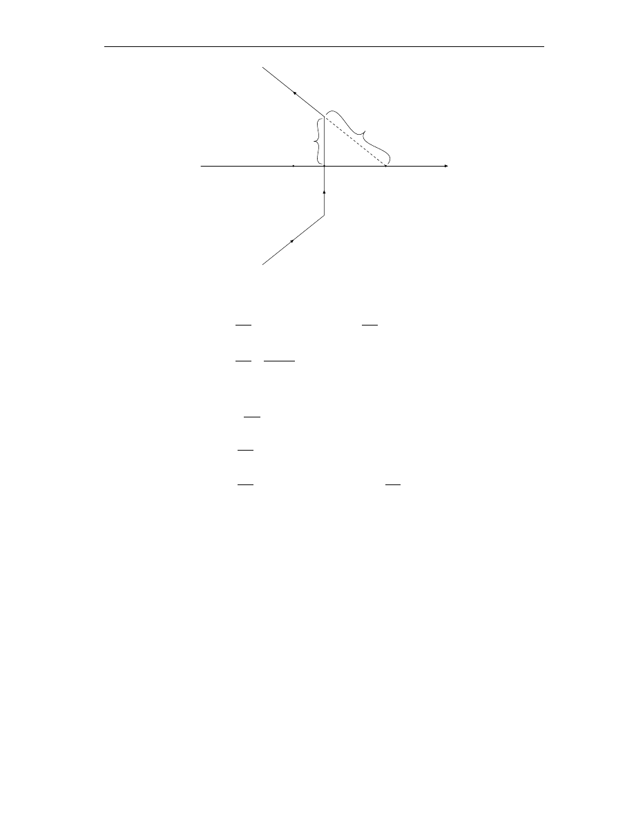
64
Chapter 5
ω
s(A) + ε
s(A)
Γ
ε
b
a
Figure 5.1: the curve Γ
ε
.
≤
M
ε
π
Z
+∞
a
e
(ω+ξ cos η)t
dξ +
M
ε
2π
Z
b
−b
e
(s(A)+ε)t
dy
≤
M
ε
π
1
| cos η|
+ b
e
(s(A)+ε)t
.
Estimate (5.2) follows for n = 0. Arguing in the same way, for t ≥ 1 we get
kAe
tA
k =
1
2πi
Z
Γ
ε
λe
tλ
R(λ, A)dλ
≤
M
ε
2π
2
Z
+∞
a
e
(ω+ξ cos η)t
dξ +
Z
b
−b
e
(s(A)+ε)t
dy
≤
M
ε
π
(| cos η|
−1
+ b)e
(s(A)+ε)t
≤
f
M
ε
t
e
(s(A)+2ε)t
.
Since ε is arbitrary, (5.2) follows also for n = 1.
From the equality A
n
e
tA
= (Ae
tA/n
)
n
we get, for n ≥ 2,
kA
n
e
tA
k
L(X)
≤ (M
1,ε
nt
−1
e
t(s(A)+ε)/n
)
n
= (M
1,ε
n)
n
t
−n
e
(s(A)+ε)t
,
and (5.2) is proved.
We remark that in the case s(A) = ω = 0, estimates (1.14) are sharper than (5.2) for
t large.
From Proposition 5.1.1 it follows that if s(A) < 0, then t 7→ e
tA
x is bounded in [0, +∞)
for every x ∈ X. In the case s(A) ≥ 0, it is interesting to characterize the elements x such
that t 7→ e
tA
x is bounded in [0, +∞). We shall see that this is possible in the case where
the spectrum of A does not intersect the imaginary axis.
5.2
Behavior of e
tA
for a hyperbolic A
In this section we assume that
σ(A) ∩ iR = ∅.
(5.3)
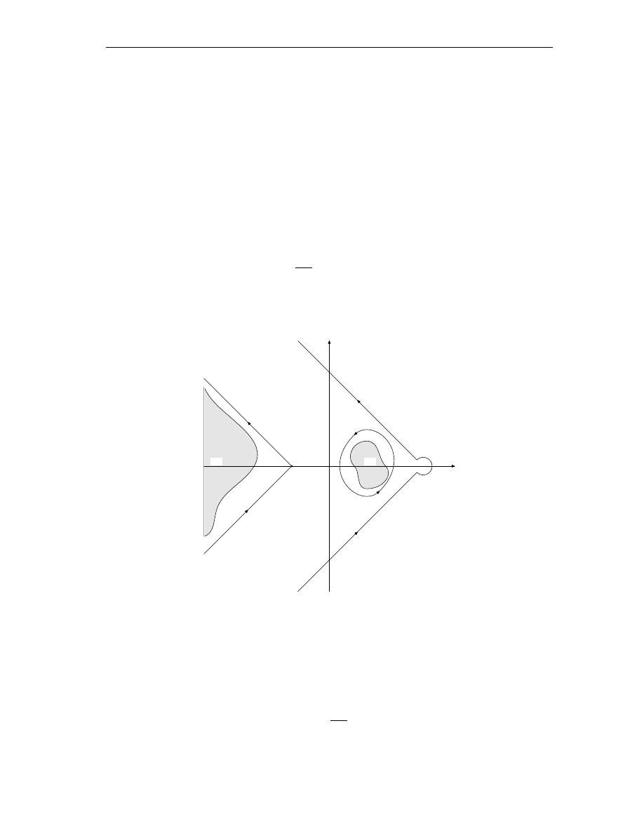
5.2. Behavior of e
tA
for a hyperbolic A
65
In this case A is said to be hyperbolic. Set σ(A) = σ
−
(A) ∪ σ
+
(A), where
σ
−
(A) = σ(A) ∩ {λ ∈ C : Re λ < 0}, σ
+
(A) = σ(A) ∩ {λ ∈ C : Re λ > 0}.
(5.4)
We write σ
+
and σ
−
, respectively for σ
+
(A) and σ
−
(A) when there is no danger of confu-
sion. Note that σ
+
is bounded. On the contrary, σ
−
may be bounded or unbounded. For
instance using Proposition 2.1.1 and Exercise 1, §1.3.5, we easily see that the spectrum of
the realization of u
00
− u in C
b
(R) is the unbounded set (−∞, −1]. On the other hand if
A ∈ L(X) then A is sectorial and σ
−
is bounded.
Since both σ
−
, σ
+
are closed we have
−ω
−
:= sup{Re λ : λ ∈ σ
−
} < 0,
ω
+
:= inf{Re λ : λ ∈ σ
+
} > 0.
(5.5)
σ
−
and σ
+
may also be empty: in this case we set ω
−
= +∞, ω
+
= +∞. Let P be the
operator defined by
P =
1
2πi
Z
γ
+
R(λ, A)dλ,
(5.6)
where γ
+
is a closed regular curve contained in ρ(A), surrounding σ
+
, oriented counter-
clockwise, with index 1 with respect to each point of σ
+
, and with index 0 with respect
to each point of σ
−
. P is called spectral projection relative to σ
+
.
γ
γ
−
−ω
γ
+
σ
+
σ
−
Figure 5.2: the curves γ
+
, γ
−
.
Proposition 5.2.1 The following statements hold.
(i) P is a projection, that is P
2
= P .
(ii) For each t ≥ 0 we have
e
tA
P = P e
tA
=
1
2πi
Z
γ
+
e
λt
R(λ, A)dλ.
(5.7)
Consequently, e
tA
(P (X)) ⊂ P (X), e
tA
((I − P )(X)) ⊂ (I − P )(X).

66
Chapter 5
(iii) P ∈ L(X, D(A
n
)) for every n ∈ N. Therefore, P (X) ⊂ D(A) and the operator
A
|P (X)
: P (X) → P (X) is bounded.
(iv) For every ω ∈ [0, ω
+
) there exists N
ω
> 0 such that for every x ∈ P (X) we have
(1)
ke
tA
xk ≤ N
ω
e
ωt
kxk, t ≤ 0.
(5.8)
(v) For each ω ∈ [0, ω
−
) there exists M
ω
> 0 such that for every x ∈ (I − P )(X) we
have
ke
tA
xk ≤ M
ω
e
−ωt
kxk, t ≥ 0.
(5.9)
Proof. Proof of (i). Let γ
+
, γ
0
+
be regular curves contained in ρ(A) surrounding σ
+
, with
index 1 with respect to each point of σ
+
, and such that γ
+
is contained in the bounded
connected component of C \ γ
0
+
. By the resolvent identity we have
P
2
=
1
2πi
2
Z
γ
0
+
R(ξ, A)dξ
Z
γ
+
R(λ, A)dλ
=
1
2πi
2
Z
γ
0
+
×γ
+
[R(λ, A) − R(ξ, A)](ξ − λ)
−1
dξdλ
=
1
2πi
2
Z
γ
+
R(λ, A)dλ
Z
γ
0
+
(ξ − λ)
−1
dξ −
1
2πi
2
Z
γ
0
+
R(ξ, A)dξ
Z
γ
+
(ξ − λ)
−1
dλ
= P.
The proof of (ii) is similar and it is left as an exercise.
Proof of (iii). Since the path γ
+
is bounded and λ 7→ R(λ, A) is continuous with values
in L(X, D(A)), then P ∈ L(X, D(A)), and
AP =
1
2πi
Z
γ
+
AR(λ, A)dλ =
1
2πi
Z
γ
+
λR(λ, A)dλ.
Therefore, AP ∈ L(X, D(A)) too. Moreover, if x ∈ D(A) then P Ax = AP x. By recur-
rence, P ∈ L(X, D(A
n
)) for every n ∈ N.
Proof of (iv). Since the part of A in P (X) is bounded and its spectrum is σ
+
(see Exercise
3, the restriction of e
tA
to P (X) may be analytically continued to (−∞, 0), using formula
(5.7). See Proposition 1.2.2.
For ω ∈ [0, ω
+
), we choose γ
+
such that inf
λ∈γ
+
Re λ = ω. Then for each t ≤ 0 and
x ∈ P (X) we have
ke
tA
xk =
1
2π
Z
γ
+
e
λt
R(λ, A)x dλ
≤ c sup
λ∈γ
+
|e
λt
| kxk = ce
ωt
kxk,
with c = (2π)
−1
|γ
+
| sup{kR(λ, A)k : λ ∈ γ
+
}, |γ
+
| = lenght of γ
+
.
1
For obvious notational reasons for each x ∈ P (X) and t < 0 we write e
tA
x instead of e
tA
|P (X)
x.

5.2. Behavior of e
tA
for a hyperbolic A
67
Proof of (v). For t small, say t < 1, estimate (5.9) is a consequence of (1.15). For t ≥ 1
we write e
tA
(I − P ) as
e
tA
(I − P ) =
1
2πi
Z
γ
−
Z
γ
+
e
λt
R(λ, A)dλ =
1
2πi
Z
γ
−
e
λt
R(λ, A)dλ,
where γ is the curve used in the definition of e
tA
(see (1.10)), γ
−
= {λ ∈ C : λ =
−ω + re
±iη
, r ≥ 0} is oriented as usual and η > π/2. See Figure 5.2. The estimate is
obtained as in the proof of Proposition 5.1.1, and it is left as an exercise.
Corollary 5.2.2 Let x ∈ X. Then
(i) We have
sup
t≥0
ke
tA
xk < +∞ ⇐⇒ P x = 0.
In this case, ke
tA
xk decays exponentially to 0 as t → +∞.
(ii) For x ∈ X, the backward Cauchy problem
(
v
0
(t) = Av(t), t ≤ 0,
v(0) = x,
(5.10)
has a bounded solution in (−∞, 0] if and only if x ∈ P (X). In this case, the bounded
solution is unique, it is given by v(t) = e
tA
x, and it decays exponentially to 0 as t → −∞.
Proof. (i) Split every x ∈ X as x = P x + (I − P )x, so that e
tA
x = e
tA
P x + e
tA
(I − P )x.
The norm of the second addendum decays exponentially to 0 as t → +∞. The norm
of the first one is unbounded if P x 6= 0. Indeed, P x = e
−tA
e
tA
P x, so that kP xk ≤
ke
−tA
k
L(P (X))
ke
tA
P xk ≤ N
ω
e
−ωt
ke
tA
P xk with ω > 0, which implies that ke
tA
P xk ≥
e
ωt
kP xk/N
ω
. Therefore t 7→ e
tA
x is bounded in R
+
if and only if P x = 0.
(ii) If x ∈ P (X), the function t 7→ e
tA
x is a strict solution of the backward Cauchy
problem, and it decays exponentially as t → −∞. Conversely, if a backward bounded
solution v does exist, then for a < t ≤ 0 we have
v(t) = e
(t−a)A
v(a) = e
(t−a)A
(I − P )v(a) + e
(t−a)A
P v(a),
where e
(t−a)A
(I − P )v(a) = (I − P )v(t), e
(t−a)A
P v(a) = P v(t). Since ke
(t−a)A
(I − P )k ≤
M
ω
e
−ω(t−a)
, letting a → −∞ we get (I − P )v(t) = 0 for each t ≤ 0, so that v is a solution
to the backward problem in P (X), v(0) = x ∈ P (X) and hence v(t) = e
tA
x.
Note that problem (5.10) is ill posed in general. Changing t to −t, it is equivalent to a
forward Cauchy problem with A replaced by −A, and −A may have very bad properties.
If A is sectorial, −A is sectorial if and only if it is bounded (see Exercise 4, §1.3.5).
The subspaces (I − P )(X) and P (X) are often called the stable subspace and the
unstable subspace, respectively.
Example 5.2.3 Let us consider again the operator A
∞
: C
2
b
(R) → C
b
(R) studied in
Subsection 2.1.1. We have ρ(A
∞
) = C \ (−∞, 0], kλR(λ, A
∞
)k ≤ (cos θ/2)
−1
, with θ =

68
Chapter 5
arg λ. In this case ω = s(A
∞
) = 0, and estimates (5.2) are worse than (1.14) for large t.
It is convenient to use (1.14), which gives
ke
tA
∞
k ≤ M
0
,
kt
k
A
k
∞
e
tA
∞
k ≤ M
k
, k ∈ N, t > 0.
Therefore e
tA
u
0
is bounded for every initial datum u
0
, and the k-th derivative with respect
to time, the 2k-th derivative with respect to x decay at least like t
−k
, as t → +∞, in the
sup norm.
Example 5.2.4 Let us now consider the problem
u
t
(t, x) = u
xx
(t, x) + αu(t, x),
t > 0, 0 ≤ x ≤ 1,
u(t, 0) = u(t, 1) = 0,
t ≥ 0,
u(0, x) = u
0
(x),
0 ≤ x ≤ 1,
(5.11)
with α ∈ R. Choose X = C([0, 1]), A : D(A) = {f ∈ C
2
([0, 1]) : f (0) = f (1) = 0} → X,
Au = u
00
+ αu. Then the spectrum of A consists of the sequence of eigenvalues
λ
n
= −π
2
n
2
+ α, n ∈ N.
In particular, if α < π
2
the spectrum is contained in the halfplane {λ ∈ C : Re λ < 0},
and by Proposition 5.1.1 the solution u(t, ·) = e
tA
u
0
of (5.11) and all its derivatives decay
exponentially as t → +∞, for any initial datum u
0
.
If α = π
2
, assumption (1.9) holds with ω = 0. This is not immediate. A possible way
to show it is to study the explicit expression of R(λ, A) (which coincides with R(λ − π
2
, B)
where B : D(A) → X, Bf = f
00
) near λ = 0, see Example 2.1.2). Here we follow another
approach. We observe that the operator A
2
u := u
00
+ π
2
u with domain D(A
2
) = {u ∈
H
2
(0, 1) : u(0) = u(1) = 0} is sectorial in L
2
(0, 1) and e
tA
2
coincides with e
tA
on C([0, 1]).
Indeed, if f ∈ C([0, 1]) any solution u ∈ D(A
2
) of λu − A
2
u = f actually belongs to
C
2
([0, 1]), so that R(λ, A) = R(λ, A
2
) in C([0, 1]) for any λ ∈ ρ(A
2
) = ρ(A). Since the
functions u
k
(x) = sin(kπx) are eigenfunctions of A
2
with eigenvalue (−k
2
+ 1)π
2
for any
k ∈ N, then (see Exercise 3, §1.3.5) e
tA
2
u
k
= e
−(k
2
−1)π
2
t
u
k
for any t ≥ 0.
If f ∈ C([0, 1]) ⊂ L
2
(0, 1), we expand it in a sine series in L
2
(0, 1),
f =
+∞
X
k=1
c
k
u
k
,
c
k
= 2
Z
1
0
f (x)u
k
(x)dx.
(5.12)
To justify the expansion, it suffices to observe that (5.12) is the Fourier series of the
function f : [−1, 1] → R which is the odd extension of f . Hence,
e
tA
f = e
tA
2
f =
+∞
X
k=1
c
k
e
−(k
2
−1)π
2
t
u
k
,
t ≥ 0,
yields
ke
tA
f k
∞
≤ 2kf k
∞
+∞
X
k=1
e
−(k
2
−1)π
2
t
,
t > 0.
which is bounded in [1, +∞). Since e
tA
is an analytic semigroup, then ke
tA
k is bounded
in [0, 1].

5.2. Behavior of e
tA
for a hyperbolic A
69
If α > π
2
, there are elements of the spectrum of A with positive real part. In the case
where α 6= n
2
π
2
for every n ∈ N, assumption (5.3) is satisfied. Let m ∈ N be such that
π
2
m
2
< α < π
2
(m + 1)
2
. By Corollary 5.2.2, the initial data u
0
such that the solution is
bounded are those which satisfy P u
0
= 0. The projection P may be written as
P =
m
X
k=1
P
k
,
(5.13)
where P
k
=
R
|λ−λ
k
|<ε
R(λ, A)dλ/(2πi), and the numbers λ
k
= −π
2
k
2
+ α, k = 1, . . . , m,
are the eigenvalues of A with positive real part, ε small. Let us show that
(P
k
f )(x) = 2 sin(kπx)
Z
1
0
sin(kπy) f (y)dy, x ∈ [0, 1].
(5.14)
For any λ 6= λ
k
expand f ∈ C([0, 1]) as in (5.12). Using Exercise 3 in §1.3.5 we get
R(λ, A)f = R(λ, A
2
)f =
+∞
X
n=1
c
n
λ − λ
n
u
n
.
Hence
P
k
f =
1
2πi
Z
|λ−λ
k
|≤ε
R(λ, A)f dλ = c
k
u
k
.
Consequently, from (5.13) and (5.14) it follows that the solution of (5.11) is bounded in
[0, +∞) if and only if
Z
1
0
sin(kπy) u
0
(y)dy = 0, k = 1, . . . , m.
Exercises 5.2.5
1. Prove statement (ii) of Proposition 5.2.1 and complete the proof of statement (v).
2. Let A be a sectorial operator in X. Define the growth bound
ω
A
= inf{γ ∈ R : ∃M > 0 s.t. ke
tA
k ≤ M e
γt
, t ≥ 0}.
Show that s(A) = ω
A
.
[Hint: show that if Re λ > ω
A
then
R(λ) =
Z
+∞
0
e
−λt
e
tA
dt
is the inverse of λI − A].
3. Prove that the spectrum of the restrictions A
+
and A
−
of A to P (X) and to (I −
P )(X) are, respectively, σ
+
and σ
−
.
[Hint: Prove that
R(λ, A
+
) =
1
2πi
Z
γ
+
R(ξ, A)
λ − ξ
dξ,

70
Chapter 5
if λ /
∈ σ
+
and γ
+
is suitably chosen, and that
R(λ, A
−
) = −
1
2πi
Z
γ
+
R(ξ, A)
λ − ξ
dξ,
if λ /
∈ σ
−
and γ
+
is suitably chosen.]
4. Let α, β ∈ R, and let A be the realization of the second order derivative in C([0, 1]),
with domain {f ∈ C
2
([0, 1]) : αf (i) + βf
0
(i) = 0, i = 0, 1}. Find s(A).
5. Let A satisfy (5.3), and let T > 0, f : [−T, 0] → P (X) be a continuous function.
Prove that for every x ∈ P (X) the backward problem
(
u
0
(t) = Au(t) + f (t), −T ≤ t ≤ 0,
u(0) = x,
has a unique strict solution in the interval [−T, 0] with values in P (X), given by the
variation of constants formula
u(t) = e
tA
x +
Z
t
0
e
(t−s)A
f (s)ds, −T ≤ t ≤ 0.
Prove that for each ω ∈ [0, ω
+
) we have
ku(t)k ≤ N
ω
kxk +
1
ω
sup
−T <t<0
kf (t)k
.
6. (A generalization of Proposition 5.2.1). Let A be a sectorial operator such that
σ(A) = σ
1
∪ σ
2
, where σ
1
is compact, σ
2
is closed, and σ
1
∩ σ
2
= ∅. Define Q by
Q =
1
2πi
Z
γ
R(λ, A)dλ,
where γ is any regular closed curve in ρ(A), around σ
1
, with index 1 with respect to
each point in σ
1
and with index 0 with respect to each point in σ
2
.
Prove that Q is a projection, that the part A
1
of A in Q(X) is a bounded operator,
and that the group generated by A
1
in Q(X) may be expressed as
e
tA
1
=
1
2πi
Z
γ
e
λt
R(λ, A)dλ.
5.3
Bounded solutions of nonhomogeneous problems in un-
bounded intervals
In this section we consider nonhomogeneous Cauchy problems in halflines. We start with
(
u
0
(t) = Au(t) + f (t), t > 0,
u(0) = u
0
,
(5.15)
where f : [0, +∞) → X is a continuous function and u
0
∈ X. We assume throughout that
A is hyperbolic, i.e. (5.3) holds, and we define σ
−
, σ
+
and ω
−
, ω
+
as in Section 5.2.

5.3. Bounded solutions of nonhomogeneous problems in unbounded intervals
71
Let P be the projection defined by (5.6). Fix once and for all a positive number ω
such that
−ω
−
< −ω < ω < ω
+
,
and let M
ω
, N
ω
be the constants given by Proposition 5.2.1(iv)(v).
Proposition 5.3.1 Let f ∈ C
b
([0, +∞); X), u
0
∈ X. Then the mild solution u of (5.15)
is bounded in [0, +∞) with values in X if and only if
P u
0
= −
Z
+∞
0
e
−sA
P f (s)ds.
(5.16)
If (5.16) holds we have
u(t) = e
tA
(I − P )u
0
+
Z
t
0
e
(t−s)A
(I − P )f (s)ds −
Z
+∞
t
e
(t−s)A
P f (s)ds, t ≥ 0.
(5.17)
Proof. For every t ≥ 0 we have u(t) = (I − P )u(t) + P u(t), where
(I − P )u(t) = e
tA
(I − P )u
0
+
Z
t
0
e
(t−s)A
(I − P )f (s)ds,
and
P u(t)
=
e
tA
P u
0
+
Z
t
0
e
(t−s)A
P f (s)ds
=
e
tA
P u
0
+
Z
+∞
0
−
Z
+∞
t
e
(t−s)A
P f (s)ds
=
e
tA
P u
0
+
Z
+∞
0
e
−sA
P f (s)ds
−
Z
+∞
t
e
(t−s)A
P f (s)ds.
For every t ≥ 0 we have
k(I − P )u(t)k
≤
M
ω
e
−ωt
k(I − P )u
0
k +
Z
t
0
M
ω
e
−ω(t−s)
ds sup
0≤s≤t
k(I − P )f (s)k
≤
M
ω
k(I − P )k
ku
0
k +
1
ω
kf k
∞
,
so that (I −P )u is bounded in [0, +∞) with values in X. The integral
R
+∞
t
e
(t−s)A
P f (s)ds
is bounded too, and its norm does not exceed
N
ω
Z
∞
t
e
ω(t−s)
ds sup
s≥0
kP f (s)k =
N
ω
ω
kP k kf k
∞
.
Hence u is bounded if and only if t 7→ e
tA
P u
0
+
R
+∞
0
e
−sA
P f (s)ds
is bounded. On the
other hand y := P u
0
+
R
+∞
0
e
−sA
P f (s)ds is an element of P (X). By Corollary 5.2.2, e
tA
y
is bounded if and only if y = 0, namely (5.16) holds. In this case, u is given by (5.17).
Now we consider a backward problem,
(
v
0
(t) = Av(t) + g(t), t ≤ 0,
v(0) = v
0
,
(5.18)

72
Chapter 5
where g : (−∞, 0] → X is a bounded and continuous function, and v
0
∈ X.
Problem (5.18) is in general ill posed, and to find a solution we will have to assume
rather restrictive conditions on the data. On the other hand, such conditions will ensure
nice regularity properties of the solutions.
Note that the variation of constants formula (4.4) is well defined only for forward
problems. Therefore, we have to make precise the concept of mild solution. A function
v ∈ C((−∞, 0]; X) is said to be a mild solution of (5.18) in (−∞, 0] if v(0) = v
0
and for
each a < 0 we have
v(t) = e
(t−a)A
v(a) +
Z
t
a
e
(t−s)A
g(s)ds, a ≤ t ≤ 0.
(5.19)
In other words, v is a mild solution of (5.18) if and only if for every a < 0, setting y = v(a),
v is a mild solution of the problem
(
v
0
(t) = Av(t) + g(t), a < t ≤ 0,
v(a) = y,
(5.20)
and moreover v(0) = v
0
.
Proposition 5.3.2 Let g ∈ C
b
((−∞, 0]; X), v
0
∈ X. Then problem (5.18) has a mild
solution v ∈ C
b
((−∞, 0]; X) if and only if
(I − P )v
0
=
Z
0
−∞
e
−sA
(I − P )g(s)ds.
(5.21)
If (5.21) holds, the bounded mild solution is unique and it is given by
v(t) = e
tA
P v
0
+
Z
t
0
e
(t−s)A
P g(s)ds +
Z
t
−∞
e
(t−s)A
(I − P )g(s)ds, t ≤ 0.
(5.22)
Proof. Assume that (5.18) has a bounded mild solution v. Then for every a < 0 and for
every t ∈ [a, 0] we have v(t) = (I − P )v(t) + P v(t), where
(I − P )v(t)
=
e
(t−a)A
(I − P )v(a) +
Z
t
a
e
(t−s)A
(I − P )g(s)ds
=
e
(t−a)A
(I − P )v(a) +
Z
t
−∞
−
Z
a
−∞
e
(t−s)A
(I − P )g(s)ds
=
e
(t−a)A
(I − P )v(a) −
Z
a
−∞
e
(a−s)A
(I − P )g(s)ds
+ v
1
(t)
=
e
(t−a)A
((I − P )v(a) − v
1
(a)) + v
1
(t).
The function
v
1
(t) :=
Z
t
−∞
e
(t−s)A
(I − P )g(s)ds, t ≤ 0,
is bounded in (−∞, 0]. Indeed,
kv
1
(t)k ≤ M
ω
sup
s≤0
k(I − P )g(s)k
Z
t
−∞
e
−ω(t−s)
ds ≤
M
ω
ω
kI − P k kgk
∞
.
(5.23)

5.4. Solutions with exponential growth and exponential decay
73
Moreover v is bounded by assumption, hence sup
a≤0
k(I − P )v(a)k < +∞. Letting a →
−∞ and using estimate (5.9) we get
(I − P )v(t) = v
1
(t), t ≤ 0.
Taking t = 0, we get (5.21). On the other hand, P v is a mild (in fact, strict) solution to
w
0
(t) = Aw(t) + P g(t), and since P v(0) = P v
0
, by Exercise 5 in §5.2.5, we have for t ≤ 0,
P v(t) = e
tA
P v
0
+
Z
t
0
e
(t−s)A
P g(s)ds.
Summing up, v is given by (5.22).
Conversely, assume that (5.21) holds, and define the function v(t) := v
1
(t) + v
2
(t),
where v
1
is defined above and v
2
(t) := e
tA
P v
0
+
R
t
0
e
(t−s)A
P g(s)ds. Then v
1
is bounded
by estimate (5.23), and v
2
is bounded by Exercise 5 in §5.2.5 again, so that v is bounded.
One checks easily that v is a mild solution of (5.20) for every a < 0, and, since (5.21)
holds, we have v(0) = P v
0
+
R
0
−∞
e
−sA
(I − P )g(s)ds = P v
0
+ (I − P )v
0
= v
0
. Then v is
a bounded mild solution to (5.18).
5.4
Solutions with exponential growth and exponential de-
cay
We now replace assumption (5.3) by
σ(A) ∩ {λ ∈ C : Re λ = ω} = ∅,
(5.24)
for some ω ∈ R. Note that (5.24) is satisfied by every ω > s(A). If I is any (unbounded)
interval and ω ∈ R we set
C
ω
(I; X) := {f : I → X continuous, kf k
C
ω
:= sup
t∈I
ke
−ωt
f (t)k < +∞}.
Let f ∈ C
ω
((0, +∞); X), g ∈ C
ω
((−∞, 0); X). Since e
t(A−ωI)
= e
−ωt
e
tA
, one checks
easily that problems (5.15) and (5.18) have mild solutions u ∈ C
ω
((0, +∞); X), v ∈
C
ω
((−∞, 0]; X) if and only if the problems
(
˜
u
0
(t) = (A − ωI)˜
u(t) + e
−ωt
f (t), t > 0,
u(0) = u
0
,
(5.25)
(
˜
v
0
(t) = (A − ωI)˜
v(t) + e
−ωt
g(t), t ≤ 0,
v(0) = v
0
,
(5.26)
have mild solutions ˜
u ∈ C
b
((0, +∞); X), ˜
v ∈ C
b
((−∞, 0]; X), and in this case we have
u(t) = e
ωt
˜
u(t), v(t) = e
ωt
˜
v(t). On the other hand, the operator ˜
A = A − ωI : D(A) → X
is sectorial and hyperbolic, hence all the results of the previous section may be applied to
problems (5.25) and (5.26). Note that such results involve the spectral projection relative
to σ
+
( ˜
A), i.e. the operator
1
2πi
Z
γ
+
R(λ, A − ωI)dλ =
1
2πi
Z
γ
+
+ω
R(z, A)dz := P
ω
,
(5.27)

74
Chapter 5
where the path γ
+
+ ω surrounds σ
ω
+
:= {λ ∈ σ(A) :
Re λ > ω} and is contained in the
halfplane {Re λ > ω}. Set moreover σ
ω
−
:= {λ ∈ σ(A) : Re λ < ω}. Note that if ω > s(A)
then P
ω
= 0.
Applying the results of Propositions 5.3.1 and 5.3.2 we get the following theorem.
Theorem 5.4.1 Under assumption (5.24) let P
ω
be defined by (5.27).
The following
statements hold:
(i) If f ∈ C
ω
((0, +∞); X) and u
0
∈ X, the mild solution u of problem (5.15) belongs to
C
ω
((0, +∞); X) if and only if
P
ω
u
0
= −
Z
+∞
0
e
−s(A−ωI)
e
−ωs
P
ω
f (s)ds,
that is
(2)
P
ω
u
0
= −
Z
+∞
0
e
−sA
P
ω
f (s)ds.
In this case u is given by (5.17), and there exists C
1
= C
1
(ω) such that
sup
t≥0
ke
−ωt
u(t)k ≤ C
1
(ku
0
k + sup
t≥0
ke
−ωt
f (t)k).
(ii) If g ∈ C
ω
((−∞, 0); X) and v
0
∈ X, problem (5.18) has a mild solution v ∈ C
ω
((−∞,
0]; X) if and only if (5.21) holds. In this case the solution is unique in C
ω
((−∞, 0]; X)
and it is given by (5.22). There is C
2
= C
2
(ω) such that
sup
t≤0
ke
−ωt
v(t)k ≤ C
2
(kv
0
k + sup
t≤0
ke
−ωt
g(t)k).
Remark 5.4.2 The definition 5.3 of a hyperbolic operator requires that X be a complex
Banach space, and the proofs of the properties of P , P e
tA
etc., rely on properties of
Banach space valued holomorphic functions.
If X is a real Banach space, we have to use the complexification of X as in Remark
1.3.17. If A : D(A) → X is a linear operator such that the complexification e
A is sectorial
in e
X, the projection P maps X into itself. To prove this claim, it is convenient to choose
as γ
+
a circumference C = {ω
0
+ re
iη
: η ∈ [0, 2π]} with centre ω
0
on the real axis. For
each x ∈ X we have
P x
=
1
2π
Z
2π
0
re
iη
R(ω
0
+ re
iη
, A)x dη
=
r
2π
Z
π
0
e
iη
R(ω
0
+ re
iη
, A) − e
−iη
R(ω
0
+ re
−iη
, A)
x dη,
and the imaginary part of the function in the integral is zero. Therefore, P (X) ⊂ X, and
consequently (I − P )(X) ⊂ X. Thus, the results of the last two sections remain true even
if X is a real Banach space.
2
Note that since σ
ω
+
is bounded, e
tA
P
ω
is well defined also for t < 0, and the results of Proposition 5.2.1
hold, with obvious modifications.

5.4. Solutions with exponential growth and exponential decay
75
Example 5.4.3 Consider the nonhomogeneous heat equation
u
t
(t, x) = u
xx
(t, x) + f (t, x),
t > 0, 0 ≤ x ≤ 1,
u(t, 0) = u(t, 1) = 0,
t ≥ 0,
u(0, x) = u
0
(x),
0 ≤ x ≤ 1,
(5.28)
where f : [0, +∞)×[0, 1] → R is continuous, u
0
is continuous and vanishes at x = 0, x = 1.
We choose as usual X = C([0, 1]), A : D(A) = {u ∈ C
2
([0, 1]) : u(0) = u(1) = 0} → X,
Au = u
00
. Since s(A) = −π
2
, then A is hyperbolic, and in this case the projection P defined
in (5.6) vanishes. Proposition 5.3.1 implies that for every bounded and continuous f and
for every u
0
∈ C([0, 1]) such that u
0
(0) = u
0
(1) = 0, the solution of (5.28) is bounded.
Note that u
0
(0) = u
0
(1) = 0 is a compatibility condition (i.e. a necessary condition) for
the solution of problem (5.28) to be continuous up to t = 0 and to satisfy u(0, ·) = u
0
.
As far as exponentially decaying solutions are concerned, we use Theorem 5.4.1(i).
Fixed ω 6= π
2
n
2
for each n ∈ N, f continuous and such that
sup
t≥0, 0≤x≤1
|e
ωt
f (t, x)| < +∞
the solution u of (5.28) satisfies
sup
t≥0, 0≤x≤1
|e
ωt
u(t, x)| < +∞
if and only if (5.16) holds. This is equivalent to (see Example 5.2.4)
Z
1
0
u
0
(x) sin(kπx) dx = −
Z
+∞
0
e
k
2
π
2
s
Z
1
0
f (s, x) sin(kπx) dx ds,
for every natural number k such that π
2
k
2
< ω. (We remark that since A sin(kπx) =
−k
2
π
2
sin(kπx) we have e
tA
sin(kπx) = e
−tπ
2
k
2
sin(kπx), for every t ∈ R).
Let us now consider the backward problem
v
t
(t, x) = v
xx
(t, x) + g(t, x),
t < 0,
0 ≤ x ≤ 1,
v(t, 0) = v(t, 1) = 0,
t ≤ 0,
v(0, x) = v
0
(x),
0 ≤ x ≤ 1,
(5.29)
to which we apply Proposition 5.3.2. Since P = 0, if g : (−∞, 0] × [0, 1] → R is bounded
and continuous, there is only a final datum v
0
such that the solution is bounded, and it is
given by (see formula (5.21))
v
0
(x) =
Z
0
−∞
e
−sA
g(s, ·)ds
(x), 0 ≤ x ≤ 1.
By Theorem 5.4.1(i), a similar conclusion holds if g is continuous and it decays exponen-
tially,
sup
t≤0, 0≤x≤1
|e
−ωt
g(t, x)| < +∞
with ω > 0.

76
Chapter 5
Exercises 5.4.4
1. Let A be a hyperbolic sectorial operator. Using Propositions 5.3.1 and 5.3.2, prove
that for every h ∈ C
b
(R; X) the problem
z
0
(t) = Az(t) + h(t), t ∈ R,
(5.30)
has a unique mild solution z ∈ C
b
(R; X), given by
z(t) =
Z
t
−∞
e
(t−s)A
(I − P )h(s)ds −
Z
∞
t
e
(t−s)A
P h(s)ds, t ∈ R.
(The definition of a mild solution of (5.30) is like the definition of a mild solution to
(5.18)). Prove that
(i) if h is constant, then z is constant;
(ii) if lim
t→+∞
h(t) = h
∞
(respectively, lim
t→−∞
h(t) = h
−∞
) then
lim
t→+∞
z(t) =
Z
+∞
0
e
sA
(I − P )h
∞
ds −
Z
0
−∞
e
sA
P h
∞
ds
(respectively, the same with +∞ replaced by −∞);
(iii) if h is T -periodic, then z is T -periodic.
2. Prove that the spectrum of the realization of the Laplacian in C
b
(R
N
) and in L
p
(R
N
)
(1 ≤ p < +∞) is (−∞, 0].
[Hint: To prove that λ ≤ 0 belongs to σ(∆), use or approximate the functions
f (x
1
, . . . , x
N
) = e
i
√
−λx
1
].
3. Let Ω be a bounded open set with a boundary of class C
2
. Let moreover
D(A
1
)
=
n
u ∈
\
1≤p<+∞
W
2,p
(Ω) : ∆u ∈ C(Ω), u = 0 on ∂Ω
o
,
D(A
2
)
=
n
u ∈
\
1≤p<+∞
W
2,p
(Ω) : ∆u ∈ C(Ω),
∂u
∂n
= 0 on ∂Ω
o
and A
i
u = ∆u for any u ∈ D(A
i
), i = 1, 2.
Show that A
1
and A
2
have compact resolvent and that s(A
1
) < 0 and s(A
2
) = 0.

Chapter 6
Nonlinear problems
6.1
Nonlinearities defined in X
Consider the initial value problem
(
u
0
(t) = Au(t) + F (t, u(t)), t > 0,
u(0) = u
0
,
(6.1)
where A : D(A) ⊂ X → X is a sectorial operator and F : [0, T ] × X → X. Throughout
this section we shall assume that F is continuous, and that for every R > 0 there is L > 0
such that
kF (t, x) − F (t, y)k ≤ Lkx − yk, t ∈ [0, T ], x, y ∈ B(0, R).
(6.2)
This means that F is Lipschitz continuous with respect to x on any bounded subset of X,
with Lipschitz constant independent of t.
As in the case of linear problems, we say that a function u defined in an interval
I = [0, τ ) or I = [0, τ ], with τ ≤ T , is a strict solution of problem (6.1) in I if it is
continuous with values in D(A) and differentiable with values in X in the interval I, and
it satisfies (6.1). We say that it is a classical solution if it is continuous with values in
D(A) and differentiable with values in X in the interval I \ {0}, it is continuous in I with
values in X, and it satisfies (6.1). We say that it is a mild solution if it is continuous with
values in X in I \ {0} and it satisfies
u(t) = e
tA
u
0
+
Z
t
0
e
(t−s)A
F (s, u(s))ds, t ∈ I.
(6.3)
By Proposition 4.1.2 every strict or classical solution satisfies (6.3).
For notational convenience, throughout this section we set
M
0
= sup
0≤t≤T
ke
tA
k
L(X)
.
(6.4)
6.1.1
Local existence, uniqueness, regularity
It is natural to solve (6.3) using a fixed point theorem to find a mild solution, and then
to show that, under appropriate assumptions, the mild solution is classical or strict.
Theorem 6.1.1 The following statements hold.
77

78
Chapter 6
(a) If u, v ∈ C
b
((0, a]; X) are mild solutions for some a ∈ (0, T ], then u ≡ v.
(b) For every u ∈ X there exist r, δ > 0, K > 0 such that for ku
0
− uk ≤ r problem
(6.1) has a mild solution u = u(·; u
0
) ∈ C
b
((0, δ]; X). The function u belongs to
C([0, δ]; X) if and only if u
0
∈ D(A).
Moreover for every u
0
, u
1
∈ B(u, r) we have
ku(t; u
0
) − u(t; u
1
)k ≤ Kku
0
− u
1
k, 0 ≤ t ≤ δ.
(6.5)
Proof. Proof of (a). Let u, v ∈ C
b
((0, a]; X) be mild solutions to (6.1) and set w = v − u.
By (6.3), the function w satisfies
w(t) =
Z
t
0
e
(t−s)A
(F (s, v(s)) − F (s, u(s))) ds,
0 ≤ t < a.
Using (6.2) with R = max{sup
0<t≤a
ku(t)k, sup
0<t≤a
kv(t)k} we see that
kw(t)k ≤ LM
0
Z
t
0
kw(s)kds.
The Gronwall lemma (see Exercise 3 in §1.2.4) implies that w = 0 in [0, a].
Proof of (b). Fix R > 0 such that R ≥ 8M
0
kuk, so that if ku
0
− uk ≤ r = R/(8M
0
)
we have
sup
0≤t≤T
ke
tA
u
0
k ≤ R/4.
Here M
0
is given by (6.4). Moreover, let L > 0 be such that
kF (t, v) − F (t, w)k ≤ Lkv − wk,
0 ≤ t ≤ T, v, w ∈ B(0, R).
We look for a mild solution belonging to the metric space
Y = {u ∈ C
b
((0, δ]; X) : ku(t)k ≤ R ∀t ∈ (0, δ]},
where δ ∈ (0, T ] has to be chosen properly. Y is the closed ball with centre at 0 and radius
R in the space C
b
((0, δ]; X), and for every v ∈ Y the function t 7→ F (t, v(t)) belongs to
C
b
((0, δ]; X). We define the operator Γ in Y , by means of
Γ(v)(t) = e
tA
u
0
+
Z
t
0
e
(t−s)A
F (s, v(s))ds, 0 ≤ t ≤ δ.
(6.6)
Clearly, a function v ∈ Y is a mild solution of (6.1) in [0, δ] if and only if it is a fixed point
of Γ.
We shall show that Γ is a contraction and maps Y into itself provided that δ is suffi-
ciently small.
Let v
1
, v
2
∈ Y . We have
kΓ(v
1
) − Γ(v
2
)k
C
b
((0,δ];X)
≤ δM
0
kF (·, v
1
(·)) − F (·, v
2
(·))k
C
b
((0,δ];X)
≤ δM
0
Lkv
1
− v
2
k
C
b
((0,δ];X)
.
(6.7)

6.1. Nonlinearities defined in X
79
Therefore, if
δ ≤ δ
0
= (2M
0
L)
−1
,
Γ is a contraction with constant 1/2 in Y . Moreover if δ ≤ δ
0
, for every v ∈ Y we have
kΓ(v)k
C
b
((0,δ];X)
≤ kΓ(v) − Γ(0)k
C
b
((0,δ];X)
+ kΓ(0)k
C((0,δ];X)
≤ R/2 + ke
·A
u
0
k
C
b
((0,δ];X)
+ M
0
δkF (·, 0)k
C
b
((0,δ];X)
≤ R/2 + R/4 + M
0
δkF (·, 0)k
C
b
((0,δ];X)
.
(6.8)
Therefore if δ ≤ δ
0
is such that
M
0
δkF (·, 0)k
C
b
((0,δ];X)
≤ R/4,
then Γ maps Y into itself, so that it has a unique fixed point in Y .
Concerning the continuity of u up to t = 0, we remark that the function t 7→ u(t)−e
tA
u
0
belongs to C([0, δ]; X), whereas by Proposition 1.3.6(i) t 7→ e
tA
u
0
belongs to C([0, δ]; X)
if and only if u
0
∈ D(A). Therefore, u ∈ C([0, δ]; X) if and only if u
0
∈ D(A).
Let us prove the statement about the dependence on the initial data. Let u
0
, u
1
belong
to B(u, r). Since Γ is a contraction with constant 1/2 in Y and both u(·; u
0
), u(·; u
1
) belong
to Y , we have
ku(·; u
0
) − u(·; u
1
)k
C
b
((0,δ];X)
≤ 2ke
·A
(u
0
− u
1
)k
C
b
((0,δ];X)
≤ 2M
0
ku
0
− u
1
k,
so that (6.5) holds, with K = 2M
0
.
6.1.2
The maximally defined solution
Now we can construct a maximally defined solution as follows. Set
τ (u
0
) = sup{a > 0 : problem (6.1) has a mild solution u
a
in [0, a]}
u(t) = u
a
(t), if t ≤ a.
Recalling Theorem 6.1.1(a), u is well defined in the interval
I(u
0
) := ∪{[0, a] : problem (6.1) has a mild solution u
a
in [0, a]},
and we have τ (u
0
) = sup I(u
0
).
Let us now prove results concerning regularity and existence in the large of the solution.
Proposition 6.1.2 Assume that there is θ ∈ (0, 1) such that for every R > 0 we have
kF (t, x) − F (s, x)k ≤ C(R)(t − s)
θ
, 0 ≤ s ≤ t ≤ T, kxk ≤ R.
(6.9)
Then, for every u
0
∈ X, u ∈ C
θ
([ε, τ (u
0
) − ε]; D(A)) ∩ C
1+θ
([ε, τ (u
0
) − ε]; X) and u
0
∈
B([ε, τ (u
0
) − ε]; D
A
(θ, ∞)) for every ε ∈ (0, τ (u
0
)/2). Moreover the following statements
hold.
(i) If u
0
∈ D(A) then u is a classical solution of (6.1).
(ii) If u
0
∈ D(A) and Au
0
+ F (0, u
0
) ∈ D(A) then u is a strict solution of (6.1).

80
Chapter 6
Proof. Let a < τ (u
0
) and 0 < ε < a. Since t 7→ F (t, u(t)) belongs to C
b
((0, a]; X), Propo-
sition 4.1.5 implies that the function v(t) :=
R
t
0
e
(t−s)A
F (s, u(s))ds belongs to C
α
([0, a]; X).
Moreover, t 7→ e
tA
u
0
belongs to C
∞
([ε, a]; X). Summing up, we find that u belongs to
C
θ
([ε, a]; X). Assumptions (6.2) and (6.9) imply that the function t 7→ F (t, u(t)) belongs
to C
θ
([ε, a]; X). Since u satisfies
u(t) = e
(t−ε)A
u(ε) +
Z
t
ε
e
(t−s)A
F (s, u(s))ds, ε ≤ t ≤ a,
(6.10)
we may apply Theorem 4.1.7 in the interval [ε, a] (see Remark 4.1.12), and we get u ∈
C
θ
([2ε, a]; D(A)) ∩ C
1+θ
([2ε, a]; X) for each ε ∈ (0, a/2), and
u
0
(t) = Au(t) + F (t, u(t)), ε < t ≤ a.
Exercise 2 in §4.1.13 implies that u
0
is bounded with values in D
A
(θ, ∞) in [2ε, a]. Since
a and ε are arbitrary, then u ∈ C
θ
([ε, τ (u
0
) − ε]; D(A)) ∩ C
1+θ
([ε, τ (u
0
) − ε]; X) for each
ε ∈ (0, τ (u
0
)/2). If u
0
∈ D(A), then t 7→ e
tA
u
0
is continuous up to 0, and statement (i)
follows.
Let us prove (ii). By Proposition 4.1.5, we already know that the function v defined
above is θ-H¨
older continuous up to t = 0 with values in X. Since u
0
∈ D(A) ⊂ D
A
(θ, ∞),
then the function t 7→ e
tA
u
0
is θ-H¨
older continuous up to t = 0, too. Therefore u is
θ-H¨
older continuous up to t = 0 with values in X, so that t 7→ F (t, u(t)) is θ-H¨
older
continuous in [0, a] with values in X. Statement (ii) follows now from Theorem 4.1.7(ii).
Proposition 6.1.3 Let u
0
be such that I(u
0
) 6= [0, T ]. Then t 7→ ku(t)k is unbounded in
I(u
0
).
Proof. Assume by contradiction that u is bounded in I(u
0
) and set τ = τ (u
0
). Then
t 7→ F (t, u(t; u
0
)) is bounded and continuous with values in X in the interval (0, τ ). Since
u satisfies the variation of constants formula (6.3), it may be continuously extended to
t = τ , in such a way that the extension is H¨
older continuous in every interval [ε, τ ], with
0 < ε < τ . Indeed, t 7→ e
tA
u
0
is well defined and analytic in the whole halfline (0, +∞),
and u − e
tA
u
0
belongs to C
α
([0, τ ]; X) for each α ∈ (0, 1) by Proposition 4.1.5.
By Theorem 6.1.1, the problem
v
0
(t) = Av(t) + F (t, v(t)), t ≥ τ,
v(τ ) = u(τ ),
has a unique mild solution v ∈ C([τ, τ + δ]; X) for some δ > 0. Note that v is continuous
up to t = τ because u(τ ) ∈ D(A) (why? See Exercise 6, §6.1.5, for a related stronger
statement).
The function w defined by w(t) = u(t) for 0 ≤ t < τ , and w(t) = v(t) for τ ≤ t ≤ τ + δ,
is a mild solution of (6.1) in [0, τ + δ]. See Exercise 2 in §6.1.5. This is in contradiction
with the definition of τ . Therefore, u cannot be bounded.
Note that the proof of proposition 6.1.3 shows also that if I(u
0
) 6= [0, T ] then τ (u
0
) =
sup I(u
0
) /
∈ I(u
0
).
The result of Proposition 6.1.3 is used to prove existence in the large when we have an
a priori estimate on the norm of u(t). Such a priori estimate is easily available for each
u
0
if f does not grow more than linearly as kxk → +∞. Note that Proposition 6.1.3 and
next Proposition 6.1.4 are quite similar to the case of ordinary differential equations.

6.1. Nonlinearities defined in X
81
Proposition 6.1.4 Assume that there is C > 0 such that
kF (t, x)k ≤ C(1 + kxk) x ∈ X, t ∈ [0, T ].
(6.11)
Let u : I(u
0
) → X be the mild solution to (6.1). Then u is bounded in I(u
0
) with values
in X. Consequently, I(u
0
) = [0, T ].
Proof. For each t ∈ I(u
0
) we have
ku(t)k ≤ M
0
ku
0
k + M
0
C
Z
t
0
(1 + ku(s)k)ds = M
0
ku
0
k + M
0
C
T +
Z
t
0
ku(s)kds
.
Applying the Gronwall lemma to the real-valued function t 7→ ku(t)k we get
ku(t)k ≤ (M
0
ku
0
k + M
0
CT )e
M
0
Ct
, t ∈ I(u
0
),
and the statement follows.
We remark that (6.11) is satisfied if F is globally Lipschitz continuous with respect to
x, with Lipschitz constant independent of t.
Exercises 6.1.5
1. Let F : [0, T ] × X → X be a continuous function. Prove that
(a) if F satisfies (6.2) and u ∈ C
b
((0, δ]; X) with 0 < δ ≤ T , then the composition
ϕ(t) := F (t, u(t)) belongs to C
b
((0, δ]; X),
(b) if F satisfies (6.2) and (6.9), and u ∈ C
θ
([a, b]; X) with 0 ≤ a < b ≤ T ,
0 < θ < 1, then the composition ϕ(t) := F (t, u(t)) belongs to C
θ
([a, b]; X).
These properties have been used in the proofs of Theorem 6.1.1 and of Proposition
6.1.2.
2. Prove that if u is a mild solution to (6.1) in an interval [0, t
0
] and v is a mild solution
to
(
v
0
(t) = Av(t) + F (t, v(t)), t
0
< t ≤ t
1
,
v(t
0
) = u(t
0
),
then the function z defined by z(t) = u(t) for 0 ≤ t ≤ t
0
, and z(t) = v(t) for
t
0
≤ t ≤ t
1
, is a mild solution to (6.1) in the interval [0, t
1
].
3. Under the assumptions of Theorem 6.1.1, for t
0
∈ (0, T ) let u(·; t
0
, x) : [t
0
, τ (t
0
, x)) →
X be the maximally defined solution to problem u
0
= Au + F (t, u), t > t
0
, u(t
0
) = x.
(a) Prove that for each a ∈ (0, τ (0, x)) we have τ (a, u(a; 0, x)) = τ (0, x) and for
t ∈ [a, τ (0; x)) we have u(t; a, u(a; 0, x)) = u(t; 0, x).
(b) Prove that if F does not depend on t, then τ (0, u(a; 0, x)) = τ (0, x) − a, and for
t ∈ [0, τ (0, x) − a) we have u(t; 0, u(a; 0, x)) = u(a + t; 0, x).
4. Under the assumptions of Theorem 6.1.1 and with the notation of Exercise 3, prove
that for each u
0
and for each b ∈ (0, τ (0, u
0
)) there are r > 0, K > 0 such that if
ku
0
− u
1
k ≤ r then τ (0, u
1
) ≥ b and ku(t; 0, u
0
) − u(t; 0, u
1
)k ≤ Kku
0
− u
1
k for each
t ∈ [0, b].
[Hint: cover the orbit {u(t; 0, u
0
) : 0 ≤ t ≤ b} with a finite number of balls as in the
statement of Theorem 6.1.1].

82
Chapter 6
5. (A variant of Theorem 6.1.1) Let O be a nonempty open set in X, and let F :
[0, T ] × O → X be a continuous function which is locally Lipschitz continuous in x,
uniformly with respect to time, i.e. for each x
0
∈ O there are r > 0, L > 0 such
that kF (t, x) − F (t, y)k ≤ Lkx − yk for each x, y ∈ B(x
0
, r). Prove that for every
u ∈ O there exist s, δ > 0, K > 0 such that for every u
0
∈ D(A) ∩ B(u, s) the
problem (6.1) has a unique mild solution u = u(·; u
0
) ∈ C([0, δ]; X). Moreover for
u
0
, u
1
∈ D(A) ∩ B(u, s) we have
ku(t; u
0
) − u(t; u
1
)k ≤ Kku
0
− u
1
k, 0 ≤ t ≤ δ.
[Hint: follow the proof of Theorem 6.1.1, with Y = B(0, ρ) ⊂ C([0, δ]; X), but now
ρ has to be small].
6. Prove that if F satisfies (6.2), then for every u
0
∈ X, the mild solution u of problem
(6.1) is bounded with values in D
A
(β, ∞) in the interval [ε, τ (u
0
) − ε], for each
β ∈ (0, 1) and ε ∈ (0, τ (u
0
)/2).
6.2
Reaction–diffusion equations and systems
Let us consider a differential system in [0, T ] × R
n
. Let d
1
, . . . , d
m
> 0 and let D be the
diagonal matrix D = diag(d
1
, . . . , d
m
). Consider the problem
(
u
t
(t, x) = D∆u(t, x) + f (t, x, u(t, x)),
t > 0,
x ∈ R
n
;
u(0, x) = u
0
(x),
x ∈ R
n
,
(6.12)
where u = (u
1
, . . . , u
m
) is unknown, and the regular function f : [0, T ] × R
n
× R
m
→ R
m
,
the bounded and continuous u
0
: R
n
→ R
m
are given.
This type of problems are often encountered as mathematical models in chemistry and
in biology. The part D∆u in the system is called the diffusion part, the numbers d
i
are
called the diffusion coefficients, f (t, x, u) is called the reaction part. Detailed treatments
of these problems may be found in the books of Rothe [14], Smoller [15], Pao [12].
Set
X = C
b
(R
n
; R
m
).
The linear operator A defined by
D(A) = {u ∈ W
2,p
loc
(R
n
; R
m
),
p ≥ 1 : u, ∆u ∈ X},
A : D(A) → X, Au = D∆u,
is sectorial in X, see Section 2.3 and Exercise 1 in §1.3.18, and
D(A) = BU C(R
n
; R
m
).
We assume that f is continuous, and that there exists θ ∈ (0, 1) such that for every R > 0
there is K = K(R) > 0 such that
|f (t, x, u) − f (s, x, v)|
R
m
≤ K((t − s)
θ
+ |u − v|
R
m
),
(6.13)
for 0 ≤ s < t ≤ T , x ∈ R
n
, u, v ∈ R
m
, |u|
R
m
, |v|
R
m
≤ R. Moreover we assume that
sup
0≤t≤T, x∈R
n
f (t, x, 0) < +∞,
(6.14)

6.2. Reaction–diffusion equations and systems
83
so that for every ϕ ∈ C
b
(R
n
; R
m
) and t ∈ [0, T ] the composition f (t, ·, ϕ(·)) is in C
b
(R
n
; R
m
).
Then we may apply the general results of Section 6.1 to get a regular solution of problem
(6.12).
Proposition 6.2.1 Under the above assumptions, for each u
0
∈ C
b
(R
n
, R
m
) there are
a maximal interval I(u
0
) and a unique solution u to (6.12) in I(u
0
) × R
n
, such that
u ∈ C(I(u
0
) × R
n
; R
m
), u
t
, D
i
u, and ∆u are bounded and continuous in the interval
[ε, τ (u
0
) − ε] for each ε ∈ (0, τ (u
0
)/2), where τ (u
0
) = sup I(u
0
).
Proof. Setting
F (t, ϕ)(x) = f (t, x, ϕ(x)), 0 ≤ t ≤ T, x ∈ R
n
, ϕ ∈ X,
the function F : [0, T ] × X → X is continuous, and it satisfies (6.2) and (6.9). Indeed, fix
any ϕ
1
, ϕ
2
∈ B(0, R) ⊂ X. Then, for all x ∈ R
n
, |ϕ
1
(x)|
R
m
≤ R, |ϕ
2
(x)|
R
m
≤ R, so that
for 0 ≤ s ≤ t ≤ T we get from (6.13)
|F (t, ϕ
1
)(x) − F (s, ϕ
2
)(x)| ≤ K((t − s)
θ
+ |ϕ
1
(x) − ϕ
2
(x)|
R
m
),
which implies
kF (t, ϕ
1
) − F (s, ϕ
2
)k
∞
≤ K((t − s)
θ
+ kϕ
1
− ϕ
2
k
∞
).
The local existence and uniqueness Theorem 6.1.1 implies that there exists a unique mild
solution t 7→ u(t) ∈ C
b
((0, δ]; X) of (6.1), that may be extended to a maximal time interval
I(u
0
).
By Proposition 6.1.2, u, u
0
, and Au are continuous in (0, τ (u
0
)) with values in X
(in fact, they are H¨
older continuous in each compact subinterval). Then the function
(t, x) 7→ u(t, x) := u(t)(x) is bounded and continuous in [0, a] × R
n
for each a ∈ I(u
0
)
(why is it continuous up to t = 0? Compare with Section 2.3, part (a), and Proposition
4.1.5), and it is continuously differentiable with respect to t in I(u
0
) \ {0} × R
n
.
Notice D(A) is continuously embedded in C
1
b
(R
n
; R
m
). This may be seen as a con-
sequence of (3.10), or it may be proved directly using estimate (3.12)(a) and then the
representation formula (1.22) for the resolvent. In any case, it follows that all the first
order space derivatives D
i
u are continuous in (0, τ (u
0
)) × R
n
too. The second order space
derivatives D
ij
u(t, ·) are in L
p
loc
(R
n
; R
m
), ∆u is continuous in I(u
0
) × R
n
, and u satisfies
(6.12).
Concerning existence in the large, Proposition 6.1.3 implies that if u is bounded in
I(u
0
) × R
n
then I(u
0
) = [0, T ].
A sufficient condition for u to be bounded is given by Proposition 6.1.4:
|f (t, x, u)|
R
m
≤ C(1 + |u|
R
m
),
t ∈ [0, T ], x ∈ R
n
, u ∈ R
m
.
(6.15)
Indeed, in this case the nonlinear function
F : [0, T ] × X → X,
F (t, ϕ)(x) = f (t, x, ϕ(x))
satisfies (6.11), for
kF (t, ϕ)k
∞
= sup
x∈R
n
|f (t, x, ϕ(x))|
R
m
≤ C(1 + kϕk
∞
).
Estimate (6.15) is satisfied if (6.13) holds with a constant K independent of R.

84
Chapter 6
Similar results hold for reaction – diffusion systems in [0, T ] × Ω, where Ω is a bounded
open set in R
n
with C
2
boundary.
The simplest case is a single equation,
(
u
t
(t, x) = ∆u(t, x) + f (t, x, u(t, x)),
t > 0,
x ∈ Ω,
u(0, x) = u
0
(x),
x ∈ Ω,
(6.16)
with Dirichlet boundary condition,
u(t, x) = 0, t > 0, x ∈ ∂Ω,
(6.17)
or Neumann boundary condition,
∂u(t, x)
∂n
= 0, t > 0, x ∈ ∂Ω.
(6.18)
Here f : [0, T ] × Ω × R → R is a regular function satisfying (6.13); u
0
: Ω → R is continuous
and satisfies the compatibility condition u
0
(x) = 0 for x ∈ ∂Ω in the case of the Dirichlet
boundary condition. Such a condition is necessary to have u continuous up to t = 0.
Again, we set our problem in the space X = C(Ω).
Since the realization of the
Laplacian in C(Ω) with homogeneous Dirichlet conditions is a sectorial operator (see
Section 2.4), then problem (6.16) has a unique classical solution in a maximal time interval.
Arguing as before, we see that if there is C > 0 such that
|f (t, x, u)| ≤ C(1 + |u|) t ∈ [0, T ], x ∈ Ω, u ∈ R
then for each initial datum u
0
the solution exists globally. But this assumption is rather
restrictive, and it is not satisfied in many mathematical models. In the next subsection
we shall see a more general assumption that yields existence in the large.
In this section, up to now we have chosen to work with real-valued functions just
because in most mathematical models the unknown u is real valued. But we could replace
C
b
(R
n
, R
m
) and C(Ω; R) by C
b
(R
n
; C
m
) and C(Ω; C) as well without any modification in
the proofs, getting the same results in the case of complex-valued data. On the contrary,
the results of the next subsection only hold for real-valued functions.
6.2.1
The maximum principle
Using the well known properties of the first and second order derivatives of real-valued
functions at relative maximum or minimum points it is possible to find estimates on the
solutions to several first or second order partial differential equations. Such techniques are
called maximum principles.
To begin with, we give a sufficient condition for the solution of (6.16)–(6.17) or of
(6.16)–(6.18) to be bounded (and hence, to exist in the large).
Proposition 6.2.2 Let Ω be a bounded open set in R
N
with C
2
boundary, and let f :
[0, T ] × Ω × R → R be a continuous function satisfying
|f (t, x, u) − f (s, x, v)| ≤ K((t − s)
θ
+ |u − v|),
for any 0 ≤ s < t ≤ T , any x ∈ Ω, any u, v ∈ R such that |u|, |v| ≤ R and for some
positive constant K = K(R). Assume moreover that
uf (t, x, u) ≤ C(1 + u
2
), 0 ≤ t ≤ T, x ∈ Ω, u ∈ R,
(6.19)

6.2. Reaction–diffusion equations and systems
85
for some C ≥ 0. Then for each initial datum u
0
the solution to (6.16)–(6.17) or to (6.16)–
(6.18) satisfies
sup
t∈I(u
0
), x∈Ω
|u(t, x)| < +∞.
If C = 0 in (6.19), then
sup
t∈I(u
0
), x∈Ω
|u(t, x)| = ku
0
k
∞
.
Proof. Fix λ > C, a < τ (u
0
) and set
v(t, x) = u(t, x)e
−λt
, 0 ≤ t ≤ a, x ∈ Ω.
The function v satisfies
v
t
(t, x) = ∆v(t, x) + f (t, x, e
λt
v(t, x))e
−λt
− λv(t, x), 0 < t ≤ a, x ∈ Ω,
(6.20)
and it satisfies the same boundary condition as u, and v(0, ·) = u
0
. Since v is continuous,
there exists (t
0
, x
0
) such that v(t
0
, x
0
) = ±kvk
C([0,a]×Ω)
. (t
0
, x
0
) is either a point of positive
maximum or of negative minimum for v. Assume for instance that (t
0
, x
0
) is a maximum
point. If t
0
= 0 we have obviously kvk
∞
≤ ku
0
k
∞
. If t
0
> 0 and x
0
∈ Ω we rewrite
(6.20) at (t
0
, x
0
) and we multiply both sides by v(t
0
, x
0
) = kvk
∞
. Since v
t
(t
0
, x
0
) ≥ 0 and
∆v(t
0
, x
0
) ≤ 0, we get
λkvk
2
∞
≤ C(1 + |e
λt
0
v(t
0
, x
0
)|
2
)e
−2λt
0
= C(1 + e
2λt
0
kvk
2
∞
)e
−2λt
0
,
so that
kvk
2
∞
≤
C
λ − C
.
Let us consider the case t
0
> 0, x
0
∈ ∂Ω. If u satisfies the Dirichlet boundary condition,
then v(t
0
, x
0
) = 0. If u satisfies the Neumann boundary condition, we have D
i
v(t
0
, x
0
) = 0
for each i, ∆v(t
0
, x
0
) ≤ 0 (see Exercise 2, §6.2.6), and we go on as in the case x
0
∈ Ω.
If (t
0
, x
0
) is a minimum point the proof is similar. Therefore we have
kvk
∞
≤ max{ku
0
k
∞
,
p
C/(λ − C)}
(6.21)
so that
kuk
∞
≤ e
λT
max{ku
0
k
∞
,
p
C/(λ − C)}
and the first statement follows.
If C = 0 we obtain kuk
∞
≤ e
λT
ku
0
k
∞
for every λ > 0 and letting λ → 0 the second
statement follows.
A similar result holds if Ω is replaced by the whole space R
N
, but the proof has to be
adapted to the noncompact domain case. Indeed, if a function v is bounded and continuous
in [0, a] × R
N
, it may have no maximum or minimum points, in general. We state this
result, without a proof, in the following proposition.
Proposition 6.2.3 Let f : [0, T ] × R
N
× R → R be a continuous function satisfying the
assumptions of Proposition 6.2.2 with Ω replaced by R
N
. Consider problem (6.12) with

86
Chapter 6
m = 1, d
1
= 1. Then for each bounded and continuous initial datum u
0
the solution to
(6.12) satisfies
sup
t∈I(u
0
), x∈R
N
|u(t, x)| < +∞,
and therefore it exists in the large. If C = 0 in (6.19), then
sup
t∈I(u
0
), x∈R
N
|u(t, x)| = ku
0
k
∞
.
Let us remark that (6.15) is a growth condition at infinity, while (6.19) is an algebraic
condition and it is not a growth condition. For instance, it is satisfied by f (t, x, u) =
λu − u
2k+1
for each k ∈ N and λ ∈ R. The sign − is important: for instance, in the
problem
u
t
= ∆u + |u|
1+ε
,
t > 0,
x ∈ Ω,
∂u
∂n
(t, x) = 0,
t > 0,
x ∈ ∂Ω,
u(0, x) = u,
x ∈ Ω,
(6.22)
with ε > 0 and constant initial datum u, the solution is independent of x and it coincides
with the solution to the ordinary differential equation
(
ξ
0
(t) = |ξ(t)|
1+ε
, t > 0,
ξ(0) = u,
which blows up in a finite time if u > 0.
In the proof of Propositions 6.2.2 and 6.2.3 we used a property of the functions ϕ ∈
D(A), where A is either the realization of the Laplacian in C
b
(R
N
) or the realization of
the Laplacian with Dirichlet or Neumann boundary condition in C(Ω): if x ∈ Ω (and also
if x ∈ ∂Ω in the case of Neumann boundary conditions) is a relative maximum point for
ϕ, then ∆ϕ(x) ≤ 0. While this is obvious if ϕ ∈ C
2
(Ω), it has to be proved if ϕ is not
twice differentiable pointwise. We provide a proof only in the case of interior points.
Lemma 6.2.4 Let x
0
∈ R
N
, r > 0, and let ϕ : B(x
0
, r) → R be a continuous function.
Assume that ϕ ∈ W
2,p
(B(x
0
, r)) for each p ∈ [1, +∞), that ∆ϕ is continuous, and that
x
0
is a maximum (respectively, minimum) point for ϕ. Then ∆ϕ(x
0
) ≤ 0 (respectively,
∆ϕ(x
0
) ≥ 0).
Proof. Assume that x
0
is a maximum point. Possibly replacing ϕ by ϕ + c, we may
assume ϕ(x) ≥ 0 for |x − x
0
| ≤ r. Let θ : R
N
→ R be a smooth function with support
contained in B(x
0
, r), such that 0 ≤ θ(x) ≤ 1 for each x, θ(x
0
) > θ(x) for x 6= x
0
, and
∆θ(x
0
) = 0. Define
e
ϕ(x) =
(
ϕ(x)θ(x),
x ∈ B(x
0
, r),
0,
x ∈ R
N
\ B(x
0
, r).
Then
e
ϕ(x
0
) is the maximum of
e
ϕ, and it is attained only at x = x
0
. Moreover,
e
ϕ and ∆
e
ϕ
are continuous in the whole R
N
and vanish outside B(x
0
, r), so that there is a sequence

6.2. Reaction–diffusion equations and systems
87
(
e
ϕ
n
)
n∈N
⊂ C
2
b
(R
N
) such that
e
ϕ
n
→
e
ϕ, ∆
e
ϕ
n
→ ∆
e
ϕ uniformly and each
e
ϕ
n
has support
contained in the ball B(x
0
, 2r). For instance, we can take
e
ϕ
n
= ηT (1/n)
e
ϕ where T (t) is
the heat semigroup defined in (2.8) and η is a smooth function with support contained in
B(x
0
, 2r) and equal to 1 in B(x
0
, r). Since x
0
is the unique maximum point of
e
ϕ, there is
a sequence (x
n
) ⊂ B(x
0
, 2r) converging to x
0
as n → ∞ such that x
n
is a maximum point
of
e
ϕ
n
, for each n. Since
e
ϕ
n
is twice continuously differentiable, we have ∆
e
ϕ
n
(x
n
) ≤ 0.
Letting n → +∞ we get ∆
e
ϕ(x
0
) ≤ 0, and consequently ∆ϕ(x
0
) ≤ 0.
If x
0
is a minimum point the proof is similar.
The maximum principle may be also used in some systems. For instance, let us consider
u
t
(t, x) = ∆u(t, x) + f (u(t, x)),
t > 0,
x ∈ Ω,
u(t, x) = 0,
t > 0,
x ∈ ∂Ω,
u(0, x) = u
0
(x),
x ∈ Ω,
where the unknown u is a R
m
-valued function, Ω is a bounded open set in R
N
with C
2
boundary, f : R
m
→ R
m
is a locally Lipschitz continuous function such that
hy, f (y)i ≤ C(1 + |y|
2
), y ∈ R
m
(6.23)
and u
0
is a continuous function vanishing on ∂Ω.
As in the case of a single equation, it is convenient to fix a ∈ (0, τ (u
0
)) and to introduce
the function v : [0, a] × Ω → R
m
, v(t, x) = u(t, x)e
−λt
with λ > C, that satisfies
v
t
(t, x) = ∆v(t, x) + f (e
λt
v(t, x))e
−λt
− λv(t, x),
t > 0,
x ∈ Ω,
v(t, x) = 0,
t > 0,
x ∈ ∂Ω,
v(0, x) = u
0
(x),
x ∈ Ω.
Instead of |v| it is better to work with ϕ(t, x) = |v(t, x)|
2
=
P
m
i=1
v
i
(t, x)
2
, which is more
regular. Let us remark that
ϕ
t
= 2hv
t
, vi,
D
j
ϕ = 2hD
j
v, vi,
∆ϕ = 2
m
X
i=1
|Dv
i
|
2
+ 2hv, ∆vi.
If (t
0
, x
0
) ∈ (0, a]×Ω is a positive maximum point for ϕ (i.e. for |v|) we have ϕ
t
(t
0
, x
0
) ≥
0, ∆ϕ(t
0
, x
0
) ≤ 0 and hence hv(t
0
, x
0
), ∆v(t
0
, x
0
)i ≤ 0. Writing the differential system at
(t
0
, x
0
) and taking the inner product with v(t
0
, x
0
) we get
0
≤ hv
t
(t
0
, x
0
), v(t
0
, x
0
)i
=
h∆v(t
0
, x
0
), v(t
0
, x
0
)i + hf (e
λt
0
v(t
0
, x
0
)), v(t
0
, x
0
)e
−λt
0
i − λ|v(t
0
, x
0
)|
2
≤ C(1 + |v(t
0
, x
0
)|
2
) − λ|v(t
0
, x
0
)|
2
so that kvk
2
∞
≤ C/(λ − C). Therefore, kvk
∞
≤ max{ku
0
k
∞
,
pC/(λ − C)}, and con-
sequently kuk
∞
≤ e
λT
max{ku
0
k
∞
,
pC/(λ − C)}, the same result as in the scalar case.
Therefore, u exists in the large.
The maximum principle is used also to prove qualitative properties of the solutions,
for instance to prove that the solutions are nonnegative for nonnegative initial data, or
nonpositive for nonpositive initial data.

88
Chapter 6
Consider for example the heat equation with Dirichlet boundary condition in a regular
bounded open set Ω ⊂ R
N
,
u
t
(t, x) = ∆u(t, x),
t > 0,
x ∈ Ω,
u(t, x) = 0,
t ≥ 0,
x ∈ ∂Ω,
u(0, x) = u
0
(x),
x ∈ Ω,
with u
0
= 0 on ∂Ω and u
0
(x) ≥ 0 for each x ∈ Ω. To show that u(t, x) ≥ 0 for each (t, x)
we consider the function v(t, x) := e
−t
u(t, x) which satisfies the same boundary condition
as u, v(0, x) = u
0
(x) and v
t
(t, x) = ∆v(t, x) − v(t, x). If v has a negative minimum at
(t
0
, x
0
), then t
0
> 0, x
0
∈ Ω and hence v
t
(t
0
, x
0
) ≤ 0, ∆v(t
0
, x
0
) ≥ 0, contradicting the
equation at (t
0
, x
0
).
More general situations, even in nonlinear problems, can be treated with the following
comparison result.
Proposition 6.2.5 Let Ω ⊂ R
N
be a bounded open set, let f ∈ C
1
(R) and let u, v ∈
C([0, a] × Ω) ∩ C
1
((0, a] × Ω) be such that, for every t ∈ (0, a], u(t, ·), v(t, ·) ∈ W
2,p
(Ω) for
every p < +∞ and ∆u(t, ·), ∆v(t, ·) ∈ C(Ω).
Assume that u
t
≥ ∆u + f (u), v
t
≤ ∆v + f (v) in (0, a] × Ω, that u(0, x) ≥ v(0, x) for
x ∈ Ω and that u(t, x) ≥ v(t, x) for (t, x) ∈ (0, a] × ∂Ω. Then u(t, x) ≥ v(t, x) in [0, a] × Ω.
Proof. The function w = u − v has the same regularity properties as u, v, and it satisfies
w
t
(t, x) ≥ ∆w(t, x) + f (u(t, x)) − f (v(t, x)) = ∆w(t, x) + h(t, x)w(t, x)
in (0, a] × Ω, where h(t, x) =
R
1
0
f
0
(v(t, x) + ξ(u(t, x) − v(t, x))) dξ is a bounded function.
Let λ > khk
∞
and set z(t, x) := e
−λt
w(t, x). Then z
t
≥ ∆z + (h − λ)z in (0, a] × Ω,
z(0, x) ≥ 0 for any x ∈ Ω, z(t, x) ≥ 0 for any t > 0, x ∈ ∂Ω so that, if z has a negative
minimum at (t
0
, x
0
), then t
0
> 0, x
0
∈ Ω and therefore z
t
(t
0
, x
0
) ≤ 0, ∆z(t
0
, x
0
) ≥ 0 in
contradiction with the differential inequality satisfied by z at (t
0
, x
0
). Therefore z ≥ 0
everywhere, i.e., u ≥ v.
As an application we consider the problem
u
t
(t, x) = ∆u(t, x) + λu(t, x) − ρu
2
(t, x),
t > 0,
x ∈ Ω,
u(t, x) = 0,
t ≥ 0,
x ∈ ∂Ω,
u(0, x) = u
0
(x),
x ∈ Ω.
(6.24)
Here λ, ρ > 0. By comparing the solution u with the function v ≡ 0, it follows that
u(t, x) ≤ 0 if u
0
(x) ≤ 0 and u(t, x) ≥ 0 if u
0
(x) ≥ 0. Therefore, by Proposition 6.2.2,
τ (u
0
) = +∞ if u
0
≥ 0. See Exercise 4, §6.2.6.
Finally, let us see a system from combustion theory. Here u and v are a concentration
and a temperature, respectively, both normalized and rescaled. The numbers Le, ε, q are
positive parameters, Le is called the Lewis number. Ω is a bounded open set in R
N
with

6.2. Reaction–diffusion equations and systems
89
C
2
boundary. The system is
u
t
(t, x) = Le ∆u(t, x) − εu(t, x)f (v(t, x)),
t > 0,
x ∈ Ω,
v
t
(t, x) = ∆v(t, x) + qu(t, x)f (v(t, x)),
t > 0,
x ∈ Ω,
∂u
∂n
(t, x) = 0, v(t, x) = 1,
t > 0,
x ∈ ∂Ω,
u(0, x) = u
0
(x), v(0, x) = v
0
(x),
x ∈ Ω,
(6.25)
f is the Arrhenius function
f (v) = e
−h/v
,
with h > 0. The initial data u
0
and v
0
are continuous nonnegative functions, with v
0
≡ 1
on ∂Ω. Replacing the unknowns (u, v) by (u, v − 1), problem (6.25) reduces to a problem
with homogeneous boundary conditions, which we locally solve using the above techniques.
The physically meaningful solutions are such that u, v ≥ 0.
Using the maximum
principle we can prove that for nonnegative initial data we get nonnegative solutions.
Let us consider u: if, by contradiction, there is a > 0 such that the restriction of u to
[0, a] × Ω has a negative minimum, say at (t
0
, x
0
) we have t
0
> 0, x
0
∈ Ω and
0 ≥ u
t
(t
0
, x
0
) = Le ∆u(t
0
, x
0
) − εu(t
0
, x
0
)f (v(t
0
, x
0
)) > 0,
a contradiction. Therefore u cannot have negative values.
To study the sign of v it is again convenient to introduce the function z(t, x) :=
e
−λt
v(t, x) with λ > 0. If there is a > 0 such that the restriction of z to [0, a] × Ω has a
negative minimum, say at (t
0
, x
0
) we have t
0
> 0, x
0
∈ Ω and
0 ≥ z
t
(t
0
, x
0
) = ∆z(t
0
, x
0
) − λz(t
0
, x
0
) + qu(t
0
, x
0
)f (z(t
0
, x
0
)e
λt
0
)e
−λt
0
> 0,
again a contradiction. Therefore, v too cannot have negative values.
Exercises 6.2.6
1. Prove the following additional regularity properties of the solution to (6.12):
(i) if u
0
∈ BU C(R
n
, R
m
), then u(t, x) → u
0
(x) as t → 0, uniformly for x in R
n
;
(ii) if for every R > 0 there is K = K(R) > 0 such that
|f (t, x, u) − f (s, y, v)|
R
m
≤ K((t − s)
θ
+ |x − y|
θ
R
n
+ |u − v|
R
m
),
for 0 ≤ s < t ≤ T , x, y ∈ R
n
, u, v ∈ R
m
, |u|
R
m
, |v|
R
m
≤ R, then all the second order
derivatives D
ij
u are continuous in I(u
0
) × R
n
.
[Hint: u
0
and F (t, u) belong to B([ε, τ (u
0
) − ε]; D
A
(θ/2, ∞)), hence u ∈ B([ε, τ (u
0
) −
ε]; C
2+θ
b
(R
N
)). To show H¨
older continuity of D
ij
u with respect to t, proceed as in
Corollary 4.1.11].
2. Let Ω be an open set in R
N
with C
1
boundary, and let x
0
∈ ∂Ω be a relative
maximum point for a C
1
function v : Ω → R. Prove that if the normal derivative of
v vanishes at x
0
then all the partial derivatives of v vanish at x
0
.
If ∂Ω and v are C
2
, prove that we also have ∆v(x
0
) ≤ 0.

90
Chapter 6
3. Construct explicitly a function θ as in the proof of Lemma 6.2.4.
4. Prove that for each continuous nonnegative initial function u
0
such that u
0
= 0 on
∂Ω, the solution to (6.24) exists in the large.
5. Show that the solution u to
u
t
(t, x) = ∆u(t, x) + u
2
(t, x) − 1,
t ≥ 0,
x ∈ Ω,
u(t, x) = 0,
t ≥ 0,
x ∈ ∂Ω
u(0, x) = u
0
(x),
x ∈ Ω
with u
0
= 0 on ∂Ω and ku
0
k
∞
≤ 1 exists in the large.
6. Let u be the solution to
u
t
(t, x) = u
xx
(t, x) + u
2
(t, x),
t ≥ 0,
x ∈ [0, 1],
u(t, 0) = u(t, 1) = 0,
t ≥ 0,
u(0, x) = u
0
(x),
x ∈ [0, 1]
with u
0
(0) = u
0
(1) = 0.
(i) Prove that if 0 ≤ u
0
(x) ≤ π
2
sin(πx) for each x ∈ [0, 1], then u exists in the large.
[Hint: compare u with v(t, x) := π
2
sin(πx)].
(ii) Set h(t) :=
R
1
0
u(t, x) sin(πx)dx and prove that h
0
(t) ≥ (π/2)h
2
− π
2
h(t) for
each t ∈ I(u
0
). Deduce that if h(0) > 2π then u blows up (i.e., ku(t, ·)k
∞
becomes
unbounded) in finite time.
6.3
Nonlinearities defined in intermediate spaces
Let A : D(A) ⊂ X → X be a sectorial operator, and let X
α
be any space of class J
α
between X and D(A), with α ∈ (0, 1). Consider the Cauchy problem
(
u
0
(t) = Au(t) + F (t, u(t)), t > 0,
u(0) = u
0
,
(6.26)
where u
0
∈ X
α
and F : [0, T ] × X
α
→ X is a continuous function, for some T > 0. The
definition of strict, classical, or mild solution to (6.26) is similar to the definition in Section
6.1.
The Lipschitz condition (6.2) is replaced by a similar assumption: for each R > 0 there
exists L = L(R) > 0 such that
kF (t, x) − F (t, y)k ≤ Lkx − yk
X
α
, t ∈ [0, T ], x, y ∈ B(0, R) ⊂ X
α
.
(6.27)
Because of the embeddings D(A) ⊂ X
α
⊂ X, then t 7→ e
tA
is analytic in (0, +∞) with
values in L(X
α
). But the norm ke
tA
k
L(X
α
)
could blow up as t → 0, see Exercise 5 in
§2.1.3. We want to avoid this situation, so we assume throughout
lim sup
t→0
ke
tA
k
L(X
α
)
< +∞.
(6.28)

6.3. Nonlinearities defined in intermediate spaces
91
It follows that ke
tA
k
L(X
α
)
is bounded on every compact interval contained in [0, +∞).
Moreover, we set
M := sup
0≤t≤T
ke
tA
k
L(X
α
)
.
(6.29)
6.3.1
Local existence, uniqueness, regularity
As in the case of nonlinearities defined in the whole X, it is convenient to look for a local
mild solution at first, and then to see that under reasonable assumptions the solution is
classical or strict.
The proof of the local existence and uniqueness theorem for mild solutions is quite
similar to the proof of Theorem 6.1.1, but we need an extension of Proposition 4.1.5. We
set
M
k,α
:= sup{t
k+α
kA
k
e
tA
k
L(X,X
α
)
: 0 < t ≤ T }, k = 0, 1, 2.
By Proposition 3.2.2(ii), M
k,α
< +∞.
In the proof of the next results, we use the following generalization of the Gronwall
lemma, whose proof may be found for instance in [9, p. 188].
Lemma 6.3.1 Let 0 ≤ a < b < ∞, and let u : [a, b] → R be a nonnegative function,
bounded in any interval [a, b − ε], integrable and such that
u(t) ≤ k + h
Z
t
a
(t − s)
−α
u(s)ds, a ≤ t ≤ b,
with 0 ≤ α < 1, h, k > 0. Then there exists C
1
> 0, independent of a, b, k such that
u(t) ≤ C
1
k,
a ≤ t < b.
Using the generalized Gronwall Lemma and Exercise 1 in §4.1.13, the proof of the
local existence and uniqueness theorem for mild solutions goes on as the proof of Theorem
6.1.1, with minor modifications.
Theorem 6.3.2 The following statements hold.
(a) If u, v ∈ C
b
((0, a]; X
α
) are mild solutions of (6.26) for some a ∈ (0, T ], then u ≡ v.
(b) For each u ∈ X
α
there are r, δ > 0, K > 0 such that if ku
0
− uk
X
α
≤ r then problem
(6.26) has a mild solution u = u(·; u
0
) ∈ C
b
((0, δ]; X
α
). The function u belongs to
C([0, δ]; X
α
) if and only if u
0
∈ D(A)
X
α
:= closure of D(A) in X
α
.
Moreover, for u
0
, u
1
∈ B(u, r) we have
ku(t; u
0
) − u(t; u
1
)k
X
α
≤ Kku
0
− u
1
k
X
α
, 0 ≤ t ≤ δ.
(6.30)
Proof. Proof of (a). The proof can be obtained arguing as in the proof of Theorem
6.1.1(a), using the generalized Gronwall lemma 6.3.1.
Proof of (b). Let M be defined by (6.29). Fix R > 0 such that R ≥ 8M kuk
X
α
, so that
if ku
0
− uk
X
α
≤ r := R/(8M ) then
sup
0≤t≤T
ke
tA
u
0
k
X
α
≤ R/4.

92
Chapter 6
Moreover, let L be such that
kF (t, v) − F (t, w)k ≤ Lkv − wk
X
α
0 ≤ t ≤ T, v, w ∈ B(0, R) ⊂ X
α
.
We look for a local mild solution of (6.26) in the metric space Y defined by
Y = {u ∈ C
b
((0, δ]; X
α
) : ku(t)k
X
α
≤ R, ∀t ∈ (0, δ]},
where δ ∈ (0, T ] will be chosen later. The space Y is the closed ball with centre at 0
and radius R in C
b
((0, δ]; X
α
), and for each v ∈ Y the function t 7→ F (t, v(t)) belongs to
C
b
((0, δ]; X). We define a nonlinear operator Γ in Y,
Γ(v)(t) = e
tA
u
0
+
Z
t
0
e
(t−s)A
F (s, v(s))ds, 0 ≤ t ≤ δ.
A function v ∈ Y is a mild solution to (6.26) in [0, δ] if and only if it is a fixed point of Γ.
We shall show that Γ is a contraction, and it maps Y into itself, provided δ is small
enough.
Let v
1
, v
2
∈ Y. By Exercise 1 in §4.1.13, Γ(v
1
) and Γ(v
2
) belong to C
b
((0, δ]; X
α
) and
kΓ(v
1
) − Γ(v
2
)k
C([0,δ];X
α
)
≤
M
0,α
1 − α
δ
1−α
kF (·, v
1
(·)) − F (·, v
2
(·))k
C
b
((0,δ];X)
≤
M
0,α
1 − α
δ
1−α
Lkv
1
− v
2
k
C
b
((0,δ];X
α
)
.
Therefore, if
δ ≤ δ
0
:=
2M
0,α
L
1 − α
−1/(1−α)
,
then Γ is a contraction in Y with constant 1/2. Moreover for each v ∈ Y and t ∈ [0, δ],
with δ ≤ δ
0
, we have
kΓ(v)k
C
b
((0,δ];X
α
)
≤ kΓ(v) − Γ(0)k
C
b
((0,δ];X
α
)
+ kΓ(0)k
C
b
((0,δ];X
α
)
≤ R/2 + ke
·A
u
0
k
C
b
((0,δ];X
α
)
+ Cδ
1−α
kF (·, 0)k
C
b
((0,δ];X)
≤ R/2 + R/4 + Cδ
1−α
kF (·, 0)k
C([0,δ];X)
.
Therefore, if δ ≤ δ
0
is such that
Cδ
1−α
kF (·, 0)k
C([0,δ];X)
≤ R/4,
then Γ maps Y into itself, and it has a unique fixed point in Y.
Concerning the continuity of u up to t = 0, we remark that the function t 7→ v(t) :=
u(t) − e
tA
u
0
is in C([0, δ]; X
α
), while t 7→ e
tA
u
0
belongs to C([0, δ]; X
α
) if and only if u
0
∈
D(A)
X
α
. See Exercise 1, §6.3.7. Therefore, u ∈ C([0, δ]; X
α
) if and only if u
0
∈ D(A)
X
α
.
The statements about continuous dependence on the initial data may be proved pre-
cisely as in Theorem 6.1.1.
The local mild solution to problem (6.26) is extended to a maximal time interval I(u
0
)
as in §6.1.1. We still define τ (u
0
) := sup I(u
0
).
Without important modifications in the proofs it is also possible to deal with regu-
larity and behavior of the solution near τ (u
0
), obtaining results similar to the ones of
Propositions 6.1.2 and 6.1.3.

6.3. Nonlinearities defined in intermediate spaces
93
Proposition 6.3.3 If there exists θ ∈ (0, 1) such that for every R > 0 we have
kF (t, x) − F (s, x)k ≤ C(R)(t − s)
θ
, 0 ≤ s ≤ t ≤ T, kxk
X
α
≤ R,
(6.31)
then the solution u of (6.26) belongs to C
θ
([ε, τ (u
0
) − ε]; D(A)) ∩ C
1+θ
([ε, τ (u
0
) − ε]; X),
and u
0
belongs to B([ε, τ − ε]; D
A
(θ, ∞)) for each ε ∈ (0, τ (u
0
)/2). Moreover, if also
u
0
∈ D(A) then u(·; u
0
) is a classical solution to (6.26). If u
0
∈ D(A) and Au
0
+F (0, u
0
) ∈
D(A) then u is a strict solution to (6.26).
Proposition 6.3.4 Let u
0
∈ X
α
be such that I(u
0
) 6= [0, T ]. Then t 7→ ku(t)k
X
α
is
unbounded in I(u
0
).
The simplest situation in which it is possible to show that ku(t)k
X
α
is bounded in
I(u
0
) for each initial datum u
0
is again the case when F grows not more than linearly
with respect to x as kxk
X
α
→ +∞.
Proposition 6.3.5 Assume that there exists C > 0 such that
kF (t, x)k ≤ C(1 + kxk
X
α
),
t ∈ [0, T ], x ∈ X
α
.
(6.32)
Let u : I(u
0
) → X
α
be the mild solution to (6.26). Then u is bounded in I(u
0
) with values
in X
α
, and hence I(u
0
) = [0, T ].
Proof. Recall that
ke
tA
xk
X
α
≤
M
0,α
t
α
kxk, x ∈ X, 0 < t ≤ T.
For each t ∈ I(u
0
) we have
ku(t)k
X
α
≤ M ku
0
k
X
α
+ M
0,α
Z
t
0
(t − s)
−α
C(1 + ku(s)k
X
α
)ds
≤ M ku
0
k
X
α
+ CM
0,α
T
1−α
1 − α
+
Z
t
0
ku(s)k
X
α
(t − s)
α
ds
.
The generalized Gronwall lemma implies the inequality
ku(t)k
X
α
≤ C
1
M ku
0
k
X
α
+
CM
0,α
T
1−α
1 − α
, t ∈ I(u
0
),
and the statement follows.
The growth condition (6.32) is apparently rather restrictive. If we have some a priori
estimate for the solution to (6.26) in the X-norm (this happens in several applications to
PDE’s), it is possible to find a priori estimates in the D
A
(θ, ∞)-norm if F satisfies suitable
growth conditions, less restrictive than (6.32). Since D
A
(θ, ∞) is continuously embedded
in X
α
for θ > α by Proposition 3.2.2, we get an a priori estimate for the solution in the
X
α
-norm, that yields existence in the large.
Proposition 6.3.6 Assume that there exists an increasing function µ : [0, +∞)
→
[0, +∞) such that
kF (t, x)k ≤ µ(kxk)(1 + kxk
γ
X
α
), 0 ≤ t ≤ T, x ∈ X
α
,
(6.33)
with 1 < γ < 1/α. Let u : I(u
0
) → X
α
be the mild solution to (6.26). If u is bounded in
I(u
0
) with values in X, then it is bounded in I(u
0
) with values in X
α
.

94
Chapter 6
Proof. Let us fix 0 < a < I(u
0
) and set I
a
= {t ∈ I(u
0
) : t ≥ a}. Since u ∈ C
b
((0, a]; X
α
)
it suffices to show that it is bounded in I
a
with values in X
α
. We show that it is bounded
in I
a
with values in D
A
(θ, ∞), when θ = αγ. This will conclude the proof by Proposition
3.2.2(i).
Set
K : sup
t∈I(u
0
)
ku(t)k.
Observe that u(a) ∈ D
A
(θ, ∞) and that it satisfies the variation of constants formula
u(t) = e
(t−a)A
u(a) +
Z
t
a
e
(t−s)A
F (s, u(s))ds,
t ∈ I(a).
Using the interpolatory estimate
kxk
X
α
≤ ckxk
1−α/θ
kxk
α/θ
D
A
(θ,∞)
,
with c = c(α, θ), that holds for every x ∈ D
A
(θ, ∞), see Exercise 4(b) in §3.2.3, we get
ku(s)k
γ
X
α
≤ cku(s)k
γ(1−α/θ)
ku(s)k
αγ/θ
D
A
(θ,∞)
≤ cK
γ(1−α/θ)
ku(s)k
D
A
(θ,∞)
, s ∈ I
a
,
so that
kF (s, u(s))k ≤ µ(K)(1 + cK
γ(1−α/θ)
ku(s)k
D
A
(θ,∞)
), s ∈ I
a
.
Let M
θ
> 0 be such that for all t ∈ (0, T ] we have kt
θ
e
tA
xk
D
A
(θ,∞)
≤ M
θ
kxk for x ∈ X,
and ke
tA
xk
D
A
(θ,∞)
≤ M
θ
kxk
D
A
(θ,∞)
for x ∈ D
A
(θ, ∞). Then for t ∈ I
a
we have
ku(t)k
D
A
(θ,∞)
≤ M
θ
ku(a)k
D
A
(θ,∞)
+M
θ
µ(K)
Z
t
a
(t − s)
−θ
(1 + cK
γ(1−α/θ)
ku(s)k
D
A
(θ,∞)
)ds, (6.34)
and the generalized Gronwall lemma implies that u is bounded in I
a
with values in
D
A
(θ, ∞).
The exponent γ = 1/α is called critical growth exponent. If γ = 1/α the above method
does not work: one should replace D
A
(αγ, ∞) by D(A) or by D
A
(1, ∞), and the integral in
(6.34) would be +∞. We already know that in general we cannot estimate the D(A)-norm
(and, similarly, the D
A
(1, ∞) norm) of v(t) = (e
tA
∗ ϕ)(t) in terms of sup kϕ(t)k.
Exercises 6.3.7
1. Show that the function t 7→ e
tA
u
0
belongs to C([0, δ]; X
α
) if and only if u
0
∈ D(A)
X
α
.
This fact has been used in Proposition 6.3.2.
2. Prove Propositions 6.3.3 and 6.3.4.
3. Let F : [0, T ] × X
α
→ X satisfy (6.27). Prove that, for any u
0
∈ X
α
, the mild
solution of (6.26) is bounded in the interval [ε, τ (u
0
) − ε] with values in D
A
(β, ∞)
for any β ∈ (0, 1) and any ε ∈ (0, τ (u
0
)/2).

6.3. Nonlinearities defined in intermediate spaces
95
6.3.2
Second order PDE’s
Let Ω be a bounded open set in R
N
with regular boundary. Let us consider the problem
u
t
(t, x) = ∆u(t, x) + f (t, x, u(t, x), Du(t, x)),
t > 0,
x ∈ Ω,
u(t, x) = 0,
t > 0,
x ∈ ∂Ω,
u(0, x) = u
0
(x),
x ∈ Ω,
(6.35)
We denote by Du the gradient of u with respect to the space variables, Du = (∂u/∂x
1
,
. . . , ∂u/∂x
N
). We assume that the function
(t, x, u, p) 7→ f (t, x, u, p), t ∈ [0, T ], x ∈ Ω, u ∈ R, p ∈ R
N
,
is continuous, H¨
older continuous with respect to t, locally Lipschitz continuous with respect
to (u, p). More precisely, we assume that there exists θ ∈ (0, 1) such that for every R > 0
there is K = K(R) > 0 such that
|f (t, x, u, p) − f (s, x, v, q)| ≤ K((t − s)
θ
+ |u − v| + |p − q|
R
N
),
(6.36)
for 0 ≤ s < t ≤ T , (u, p), (v, q) ∈ B(0, R) ⊂ R
N +1
.
We choose as X the space of the continuous functions in Ω. Then the realization A of
the Laplacian with Dirichlet boundary condition is sectorial in X, and Theorem 3.1.10(ii)
implies that for α ∈ (1/2, 1) we have
D
A
(α, ∞) = C
2α
0
(Ω) = {u ∈ C
2α
(Ω) : u(x) = 0 x ∈ ∂Ω}.
Therefore, choosing X
α
= D
A
(α, ∞) with α > 1/2, the nonlinear function
F (t, ϕ)(x) = f (t, x, ϕ(x), Dϕ(x))
is well defined in [0, T ] × X
α
, with values in X. We recall that the part of A in D
A
(α, ∞)
is sectorial in D
A
(α, ∞) and hence (6.28) holds.
We could also take α = 1/2 and X
1/2
= {ϕ ∈ C
1
(Ω) : ϕ = 0 on ∂Ω}. Indeed, it is
possible to show that assumption (6.28) holds in such a space.
If the initial datum u
0
is in C
2α
0
(Ω) with α ∈ (1/2, 1), we may rewrite problem (6.35) in
the abstract formulation (6.26). The local existence and uniqueness theorem 6.3.2 yields
a local existence and uniqueness result for problem (6.35).
Proposition 6.3.8 Under the above assumptions, for ach u
0
∈ C
2α
0
there exists a maxi-
mal time interval I(u
0
) such that problem (6.35) has a unique solution u : I(u
0
) × Ω → R,
such that u and the space derivatives D
i
u, i = 1, . . . , N , are continuous in I(u
0
) × Ω, and
u
t
, ∆u are continuous in (ε, τ (u
0
)−ε)×Ω for any ε ∈ (0, τ (u
0
)/2). Here τ (u
0
) = sup I(u
0
),
as usual.
Proof. With the above choice, the assumptions of Theorem 6.3.2 are satisfied, so that
problem (6.35) has a unique local solution u = u(t; u
0
) ∈ C
b
((0, a]; C
2α
0
(Ω)) for each a <
τ (u
0
), that belongs to C([ε, τ (u
0
)−ε]; D(A)) ∩ C
1
([ε, τ (u
0
)−ε]; X) for each ε ∈ (0, τ (u
0
)),
by Proposition 6.3.3. Consequently, the function
u(t, x; u
0
) = u(t; u
0
)(x), 0 ≤ t ≤ δ, x ∈ Ω,

96
Chapter 6
is a solution to (6.35) with the claimed regularity properties. The continuity of the first
order space derivatives D
i
u up to t = 0 follows from Exercise 4(c) in §3.2.3 and from the
continuous embedding D
A
(β, ∞) ⊂ C
1
(Ω) for β > 1/2.
By Proposition 6.3.5, a sufficient condition for existence in the large is
|f (t, x, u, p)| ≤ C(1 + |u| + |p|
R
N
),
t ∈ [0, T ], x ∈ Ω, u ∈ R, p ∈ R
N
.
(6.37)
Indeed, in this case the nonlinear function
F : [0, T ] × X
α
→ X,
F (t, u)(x) = f (t, x, u(x), Du(x))
satisfies condition (6.32).
In general, one can find an a priori estimate for the sup norm of the solution provided
that
uf (t, x, u, 0) ≤ C(1 + u
2
), 0 ≤ t ≤ T, x ∈ Ω, u ∈ R.
(6.38)
Indeed, in this case we may use again the procedure of Proposition 6.2.2. Once we know
that u is bounded in I(u
0
) with values in X, we may use Proposition 6.3.6. Assume that
there is an increasing function µ : [0, +∞) → [0, +∞) such that for some ε > 0 we have
|f (t, x, u, p)| ≤ µ(|u|)(1 + |p|
2−ε
), 0 ≤ t ≤ T, x ∈ Ω, u ∈ R, p ∈ R
N
.
(6.39)
Then the nonlinearity
F (t, u)(x) = f (t, x, u(x), Du(x)), 0 ≤ t ≤ T, u ∈ C
2α
0
(Ω), x ∈ Ω,
satisfies (6.33) with γ = 2 − ε, because
kF (t, u)k
∞
≤ µ(kuk
∞
)(1 + kuk
2−ε
C
1
) ≤ µ(kuk
∞
)(1 + kuk
2−ε
C
2α
), 0 ≤ t ≤ T, u ∈ C
2α
0
(Ω).
Then, Proposition 6.3.6 yields existence in the large provided that (2 − ε)α < 1.
A class of equations that fits the general theory are the equations in divergence form,
u
t
=
N
X
i=1
D
i
(ϕ
i
(u) + D
i
u) = ∆u +
N
X
i=1
ϕ
0
i
(u)D
i
u,
t > 0,
x ∈ Ω,
u(t, x) = 0,
t > 0,
x ∈ ∂Ω,
u(0, x) = u
0
(x),
x ∈ Ω,
(6.40)
for which we have existence in the large for all initial data if the functions ϕ
i
: R → R are
differentiable with locally Lipschitz continuous derivatives. Indeed, the function
f (t, x, u, p) =
N
X
i=1
ϕ
0
i
(u)p
i
satisfies conditions (6.38) and (6.39).

6.3. Nonlinearities defined in intermediate spaces
97
6.3.3
The Cahn-Hilliard equation
Let us consider a one dimensional Cahn-Hilliard equation,
u
t
=
− u
xx
+ f (u)
xx
,
t > 0,
x ∈ [0, 1],
u
x
(t, 0) = u
x
(t, 1) = u
xxx
(t, 0) = u
xxx
(t, 1) = 0,
t > 0,
u(0, x) = u
0
(x),
x ∈ [0, 1],
(6.41)
under the following assumptions on f and u
0
:
f ∈ C
3
(R), f has a nonnegative primitive Φ,
u
0
∈ C
2
([0, 1]), u
0
0
(0) = u
0
0
(1) = 0.
Assumption f ∈ C
3
(R) and the assumptions on u
0
are sufficient to obtain a local solution.
The positivity of a primitive of f will be used to get a priori estimates on the solution
that guarantee existence in the large.
Set X = C([0, 1]) and
D(B) = {ϕ ∈ C
2
([0, 1]) : ϕ
0
(0) = ϕ
0
(1) = 0}, Bϕ = ϕ
00
,
D(A) = {ϕ ∈ C
4
([0, 1]) : ϕ
0
(0) = ϕ
0
(1) = ϕ
000
(0) = ϕ
000
(1) = 0}, Aϕ = −ϕ
0000
.
The operator A has a very special form; specifically A = −B
2
, where B is sectorial by
Exercise 4, §2.1.3, and (1.9) holds with any θ ∈ (π/2, π). Then A is sectorial in X by
Exercise 1, §2.2.4, and D(B) is of class J
1/2
between X and D(A) by Exercise 1, §3.2.3.
Therefore we may choose
α = 1/2, X
1/2
= D(B).
Note that both D(B) and D(A) are dense in X. Since B commutes with R(λ, A) on D(B)
for each λ ∈ ρ(A), then it commutes with e
tA
on D(B), and for each ϕ ∈ D(B) and
t ∈ [0, T ] we have
ke
tA
ϕk
D(B)
= ke
tA
ϕk
∞
+
d
2
dx
2
e
tA
ϕ
∞
= ke
tA
ϕk
∞
+ ke
tA
ϕ
00
k
∞
≤ M
0
kϕk
D(B)
,
for some M
0
> 0, so that condition (6.28) is satisfied.
The function
F : X
1/2
→ X,
F (ϕ) =
d
2
dx
2
f (ϕ) = f
0
(ϕ)ϕ
00
+ f
00
(ϕ)(ϕ
0
)
2
is Lipschitz continuous on each bounded subset of X
1/2
, because f
00
is locally Lipschitz
continuous.
Theorem 6.3.2 implies that for each u
0
∈ D(B) there is a maximal τ = τ (u
0
) > 0 such
that problem (6.41) has a unique solution u : [0, τ ) × [0, 1] → R, such that u, u
x
, u
xx
are
continuous in [0, τ ) × [0, 1], and u
t
, u
xxx
, u
xxxx
are continuous in (0, τ ) × [0, 1]. Notice
that, since D(B) is dense in X, then D(A) = D(B
2
) is dense in D(B). In other words,
the closure of D(A) in X
1/2
is the whole X
1/2
.

98
Chapter 6
Since we have a fourth order differential equation, the maximum principles are not of
help to prove that u is bounded. We shall prove that the norm ku
x
(t, ·)k
L
2
is bounded in
I(u
0
); this will imply that u is bounded in I(u
0
) through a Poincar´
e-Sobolev inequality.
Since u
t
= (−u
xx
+ f (u))
xx
for each t > 0, for ε ∈ (0, τ (u
0
)) we have
Z
1
0
(u(t, x) − u(ε, x))dx =
Z
t
ε
dt
Z
1
0
u
t
(s, x)dx = 0, ε ≤ t < τ (u
0
).
(6.42)
Letting ε tend to 0 we get
Z
1
0
u(t, x)dx =
Z
1
0
u
0
(x)dx, 0 < t < τ (u
0
),
so that the mean value of u(t, ·) is a constant, independent of t
(1)
.
Fix again ε ∈ (0, τ (u
0
)), multiply both sides of the equation by −u
xx
+ f (u), and
integrate over [ε, t] × [0, 1] for t ∈ (ε, τ (u
0
)). We get
−
Z
t
ε
Z
1
0
u
t
u
xx
ds dx +
Z
t
ε
Z
1
0
u
t
f (u)ds dx =
Z
t
ε
Z
1
0
(−u
xx
+ f (u))(−u
xx
+ f (u))
xx
ds dx
Note that we may integrate by parts with respect to x in the first integral, because u
tx
exists and it is continuous in [ε, t] × [0, 1], see Exercise 2(a), §6.3.9. Hence, we integrate
by parts in the first integral, we rewrite the second integral recalling that f = Φ
0
, and we
integrate by parts in the third integral too. We get
Z
t
ε
Z
1
0
u
x
(s, x)u
tx
(s, x)ds dx +
Z
t
ε
d
ds
Z
1
0
Φ(u(s, x))dx ds
= −
Z
t
ε
Z
1
0
(−u
xx
(s, x) + f (u(s, x))
x
2
dx ds
so that
1
2
Z
1
0
u
x
(t, x)
2
dx −
1
2
Z
1
0
u
x
(ε, x)
2
dx +
Z
1
0
[Φ(u(t, x) − Φ(u(ε, x))]dx ≤ 0,
and letting ε → 0 we get
ku
x
(t, ·)k
2
L
2
+ 2
Z
1
0
Φ(u(t, x))dx ≤ ku
0
0
k
2
L
2
+ 2
Z
1
0
Φ(u
0
(x))dx, 0 < t < τ (u
0
).
Since Φ is nonnegative, then u
x
(t, ·) is bounded in L
2
for t ∈ I(u
0
). Since u(t, ·) has
constant mean value, inequality (6.45) yields that u(t, ·) is bounded in the sup norm.
Now we may use Proposition 6.3.6, because F satisfies (6.33) with γ = 1. Indeed, for
each ϕ ∈ X
1/2
we have
kF (ϕ)k ≤
sup
|ξ|≤kϕk
∞
|f
0
(ξ)| · kϕ
00
k
∞
+
sup
|ξ|≤kϕk
∞
|f
00
(ξ)| · kϕ
0
k
2
∞
≤
sup
|ξ|≤kϕk
∞
|f
0
(ξ)| · kϕ
00
k
∞
+
sup
|ξ|≤kϕk
∞
|f
00
(ξ)| · Ckϕk
∞
kϕ
00
k
∞
≤ µ(kϕk)kϕk
D(B)
where µ(s) = max{sup
|ξ|≤s
|f
0
(ξ)|, Cs sup
|ξ|≤s
|f
00
(ξ)|}, and C is the constant in Exercise
2(b), §6.3.9. Therefore F has subcritical growth (the critical growth exponent is 2). By
Proposition 6.3.6, the solution exists in the large.
1
We take ε > 0 in (6.42) because our solution is just classical and it is not strict in general, so that it
is not obvious that u
t
is in L
1
((0, t) × (0, 1)).

6.3. Nonlinearities defined in intermediate spaces
99
6.3.4
The Kuramoto-Sivashinsky equation
This equation arises as a mathematical model in a two dimensional combustion phe-
nomenon. At time t, the combustion takes place along an unknown curve with equation
x = ξ(t, y), and the open set {(x, y) ∈ R
2
: x < ξ(t, y)} is the fresh region, the open set
{(x, y) ∈ R
2
: x > ξ(t, y)} is the burnt region at time t. As time increases, the curve
moves to the left, and under suitable assumptions the function Φ(t, y) = ξ(t, y) + t satisfies
the Kuramoto-Sivashinsky equation
Φ
t
(t, y) + 4Φ
yyyy
(t, y) + Φ
yy
(t, y) +
1
2
(Φ
y
)
2
= 0, t ≥ 0, y ∈ R.
(6.43)
The Cauchy problem
Φ(0, y) = Φ
0
(y), y ∈ R
(6.44)
for equation (6.43) may be treated with the methods of §6.3.3. Set
X = C
b
(R),
and
A : D(A) = C
4
b
(R),
Au = −4u
0000
− u
00
.
To prove that A is sectorial, it is convenient to write it as
A = −4B
2
− B
where B is the realization of the second order derivative in X, that is sectorial by §2.1.1.
By Exercise 1, §2.2.4, −4B
2
is sectorial, and by Exercise 1, §3.2.3, the domain D(B) is of
class J
1/2
between X and D(B
2
). Then Proposition 3.2.2(iii) yields that A is sectorial.
Since the nonlinearity
1
2
(Φ
y
)
2
depends on the first order space derivative, it is conve-
nient to choose α = 1/4 and
X
1/4
:= C
1
b
(R).
Such a space belongs to the class J
1/4
between X and D(A), by Exercise 3, §3.2.3. The
nonlinear function
F (u)(y) = −
1
2
(u
0
(y))
2
, u ∈ X
1/4
, y ∈ R,
is Lipschitz continuous on the bounded subsets of X
1/4
, and it is not hard to prove that
ke
tA
k
L(X
1/4
)
≤ ke
tA
k
L(X)
for each t > 0, see Exercise 4 below.
So, we may rewrite problem (6.43)–(6.44) in the form (6.26), with F independent of
t. All the assumptions of Theorem 6.3.2 are satisfied. Moreover, X
1/4
is contained in
D(A) = BU C(R), since all the elements of X
1/4
are bounded and Lipschitz continuous
functions.
It follows that for each Φ
0
∈ C
1
b
(R) problem (6.43)–(6.44) has a unique classical solution
Φ(t, y), defined for t in a maximal time interval [0, τ (Φ
0
)) and for y in R, such that for
every a ∈ (0, τ (Φ
0
)), Φ ∈ C
b
([0, a] × R), and there exist Φ
t
, Φ
yyyy
∈ C((0, a] × R), that are
bounded in each [ε, a] × R with 0 < ε < a.
Exercises 6.3.9
1. Prove that the conclusions of Proposition 6.2.2 hold for the solution of problem
(6.35), provided that (6.38) holds.

100
Chapter 6
2. (a) Referring to §6.3.3, prove that u
tx
exists and it is continuous in [ε, τ − ε] × [0, 1]
for each ε ∈ (0, τ /2).
[Hint: use Proposition 6.3.3 to get t 7→ u
t
(t, ·) ∈ B([ε, τ − ε]; D
A
(θ, ∞)) for each
θ ∈ (0, 1), and then Exercise 4(c), §3.2.3, to conclude].
(b) Prove that there is C > 0 such that for each ϕ ∈ C
2
([0, 1]) satisfying ϕ
0
(0) =
ϕ
0
(1) = 0 we have
kϕ
0
k
2
∞
≤ Ckϕk
∞
kϕ
00
k
∞
.
3. Prove the inequality
kϕ −
Z
1
0
ϕ(y)dyk
∞
≤
Z
1
0
(ϕ
0
(x))
2
dx
1/2
,
(6.45)
for each ϕ ∈ C
1
([0, 1]).
4. Referring to §6.3.4, prove that ke
tA
k
L(X
1/4
)
≤ ke
tA
k
L(X)
, for every t > 0.
[Hint: show that e
tA
commutes with the first order derivative on X
1/4
. For this
purpose, use Exercise 1.3.18].

Chapter 7
Behavior near stationary solutions
7.1
The principle of linearized stability
Let A : D(A) ⊂ X → X be a sectorial operator. We use the notation of Chapter 6, so X
α
is a space of class J
α
between X and D(A), that satisfies (6.28), and 0 < α < 1.
Let us consider the nonlinear equation
u
0
(t) = Au(t) + F (u(t)), t > 0,
(7.1)
where F : X → X, or F : X
α
→ X satisfies the assumptions of the local existence
Theorems 6.1.1 or 6.3.2. Throughout this section we assume that F (0) = 0, so that
problem (7.1) admits the stationary (:= constant in time) solution u ≡ 0, and we study
the stability of the null solution.
From the point of view of the stability, the case where F is defined in X
α
does not
differ much from the case where it is defined in the whole space X, and they will be treated
together, setting X
0
:= X and considering α ∈ [0, 1).
In any case we assume that the Lipschitz constant
K(ρ) := sup
kF (x) − F (y)k
kx − yk
X
α
: x, y ∈ B(0, ρ) ⊂ X
α
(7.2)
satisfies
lim
ρ→0
+
K(ρ) = 0.
(7.3)
This implies that F is Fr´
echet differentiable at 0, with null derivative.
We recall that if X, Y are Banach spaces and y ∈ Y , we say that a function G defined
in a neighborhood of y with values in X is Fr´
echet differentiable at y if there exists a linear
bounded operator L ∈ L(Y, X) such that
lim
h→0
kG(y + h) − G(y) − Lhk
X
khk
Y
= 0.
In this case, L is called the derivative of G at y and we set L = G
0
(y). If O ⊂ Y is an
open set, we say that G : O → X is continuously differentiable in O if it is differentiable
at each y ∈ O and the function G
0
: O → L(Y, X) is continuous in O.
It is clear that if F is Fr´
echet continuously differentiable in a neighborhood of 0, and
F
0
(0) = 0, then lim
ρ→0
+
K(ρ) = 0.
101

102
Chapter 7. Behavior near stationary solutions
By Theorem 6.1.1 (if α = 0) or Theorem 6.3.2 (if α ∈ (0, 1)), for every initial datum
u
0
∈ X
α
the Cauchy problem for equation (7.1) has a unique solution u(·; u
0
) defined in a
maximal time interval [0, τ (u
0
)).
Definition 7.1.1 We say that the null solution of (7.1) is stable (in X
α
) if for every
ε > 0 there exists δ > 0 such that
u
0
∈ X
α
, ku
0
k
X
α
≤ δ =⇒ τ (u
0
) = +∞, ku(t; u
0
)k
X
α
≤ ε, ∀t ≥ 0.
The null solution of (7.1) is said to be asymptotically stable if it is stable and moreover
there exists δ
0
> 0 such that if ku
0
k
X
α
≤ δ
0
then lim
t→+∞
ku(t; u
0
)k
X
α
= 0.
The null solution of (7.1) is said to be unstable if it is not stable.
The principle of linearized stability says that in the noncritical case s(A) 6= 0 the
null solution to the nonlinear problem (7.1) has the same stability properties of the null
solution to the linear problem u
0
= Au. Note that by assumption (7.3) the linear part of
Ax + F (x) near x = 0 is just Ax, so that the nonlinear part F (u) in problem (7.1) looks
like a small perturbation of the linear part u
0
= Au, at least for solutions close to 0. In
the next two subsections we make this argument rigorous.
The study of the stability of other possible stationary solutions, that is of the u ∈ D(A)
such that
Au + F (u) = 0,
can be reduced to the case of the null stationary solution by defining a new unknown
v(t) = u(t) − u,
and studying the problem
v
0
(t) = e
Av(t) + e
F (v(t)), t > 0,
where e
A = A + F
0
(u) and e
F (v) = F (v + u) − F (u) − F
0
(u)v, provided that F is Fr´
echet
differentiable at u. Note that in this case the Fr´
echet derivative of e
F vanishes at 0.
7.1.1
Linearized stability
The main assumption is
s(A) < 0.
(7.4)
(The spectral bound s(A) is defined in (5.1)). In the proof of the linearized stability
theorem we shall use the next lemma, which is a consequence of Proposition 5.1.1.
Lemma 7.1.2 Let (7.4) hold, and fix ω ∈ [0, −s(A)).
If f ∈ C
−ω
((0, +∞); X) and
x ∈ X
α
then the function
v(t) = e
tA
x +
Z
t
0
e
(t−s)A
f (s)ds, t > 0,
belongs to C
−ω
((0, +∞); X
α
), and there is a constant C = C(ω) such that
sup
t>0
e
ωt
kv(t)k
X
α
≤ C(kxk
X
α
+ sup
t>0
e
ωt
kf (t)k).

7.1. The principle of linearized stability
103
Proof. By Proposition 5.1.1, for each ω ∈ [0, −s(A)) there is M (ω) > 0 such that
ke
tA
k
L(X)
≤ M (ω)e
−ωt
, for every t > 0. Therefore, for t ≥ 1,
ke
tA
k
L(X,X
α
)
≤ ke
A
k
L(X,X
α
)
ke
(t−1)A
k
L(X)
≤ Ce
−ωt
(7.5)
with C = M (ω)e
ω
ke
A
k
L(X,X
α
)
, while for 0 < t < 1 we have ke
tA
k
L(X,X
α
)
≤ Ct
−α
for some
constant C > 0, by Proposition 3.2.2(ii). Since ω ∈ [0, −s(A)) is arbitrary, this implies
sup
t>0
e
ωt
t
α
ke
tA
k
L(X,X
α
)
:= C
ω
< +∞.
Since X
α
is continuously embedded in X, (7.5) implies also that ke
tA
k
L(X
α
)
≤ b
Ce
−ωt
for
t ≥ 1 and some positive constant b
C. Since ke
tA
k
L(X
α
)
is bounded for t ∈ (0, 1) by a
constant independent of t by assumption (6.28), we get
sup
t>0
e
ωt
ke
tA
k
L(X
α
)
:= e
C
ω
< +∞.
Therefore ke
tA
xk
X
α
≤ e
C
ω
e
−ωt
kxk
X
α
, and for any fixed ω
0
∈ (ω, −s(A)),
ke
ωt
(e
tA
∗ f )(t)k
X
α
≤ C
ω
0
e
ωt
Z
t
0
e
−ω
0
s
s
α
kf (t − s)kds ≤
C
ω
0
Γ(1 − α)
(ω
0
− ω)
1−α
sup
r>0
e
ωr
kf (r)k,
for every t > 0, and the statement follows.
Theorem 7.1.3 Let A satisfy (7.4), and let F : X
α
→ X be Lipschitz continuous in a
neighborhood of 0 and satisfy (7.3). Then for every ω ∈ [0, −s(A)) there exist positive
constants M = M (ω), r = r(ω) such that if u
0
∈ X
α
, ku
0
k
X
α
≤ r, we have τ (u
0
) = +∞
and
ku(t; u
0
)k
X
α
≤ M e
−ωt
ku
0
k
X
α
, t ≥ 0.
(7.6)
Therefore the null solution is asymptotically stable.
Proof. Let Y be the closed ball centered at 0 with small radius ρ in the space C
−ω
((0, +∞);
X
α
), namely
Y = {u ∈ C
−ω
((0, +∞); X
α
) : sup
t≥0
ke
ωt
u(t)k
X
α
≤ ρ}.
We look for the mild solution to (7.1) with initial datum u
0
as a fixed point of the operator
G defined on Y by
(Gu)(t) = e
tA
u
0
+
Z
t
0
e
(t−s)A
F (u(s))ds, t ≥ 0.
(7.7)
If u ∈ Y , by (7.2) we get
kF (u(t))k = kF (u(t)) − F (0)k ≤ K(ρ)ku(t)k
X
α
≤ K(ρ)ρe
−ωt
, t ≥ 0,
(7.8)
so that F (u(·)) ∈ C
−ω
((0, +∞); X). Using Lemma 7.1.2 we get
kGuk
C
−ω
((0,+∞);X
α
)
≤ C ku
0
k
X
α
+ kF (u(·))k
C
−ω
((0,+∞);X)
≤ C (ku
0
k
X
α
+ ρK(ρ)) .
(7.9)

104
Chapter 7. Behavior near stationary solutions
If ρ is so small that
K(ρ) ≤
1
2C
,
and
ku
0
k
X
α
≤ r :=
ρ
2C
,
then Gu ∈ Y . Moreover, for u
1
, u
2
∈ Y we have, again by Lemma 7.1.2,
kGu
1
− Gu
2
k
C
−ω
((0,+∞);X
α
)
≤ CkF (u
1
(·)) − F (u
2
(·))k
C
−ω
((0,+∞);X)
,
and (7.2) yields
kF (u
1
(t)) − F (u
2
(t))k ≤ K(ρ)ku
1
(t) − u
2
(t)k
X
α
, t > 0.
It follows that
kGu
1
− Gu
2
k
C
−ω
((0,+∞);X
α
)
≤
1
2
ku
1
− u
2
k
C
−ω
((0,+∞);X
α
)
,
so that G is a contraction with constant 1/2. Consequently there exists a unique fixed point
of G in Y , which is the solution of (7.1) with initial datum u
0
. Note that the Contraction
Theorem gives a unique solution in Y , but we already know by Theorems 6.1.1 and 6.3.2
that the mild solution is unique.
Moreover from (7.8), (7.9) we get
kuk
C
−ω
= kGuk
C
−ω
≤ C(ku
0
k
X
α
+ K(ρ)kuk
C
−ω
) ≤ Cku
0
k
X
α
+
1
2
kuk
C
−ω
which implies (7.6), with M = 2C.
Remark 7.1.4 Note that any mild solution to problem (7.1) is smooth for t > 0. Pre-
cisely, Proposition 6.1.2 if α = 0 and Proposition 6.3.3 if α > 0 imply that for each
θ ∈ (0, 1) and for each interval [a, b] ⊂ (0, τ (u
0
)), the restriction of u(·; u
0
) to [a, b] belongs
to C
1+θ
([a, b]; X) ∩ C
θ
([a, b]; D(A)).
7.1.2
Linearized instability
Assume now that
σ
+
(A) := σ(A) ∩ {λ ∈ C : Re λ > 0} 6= ∅,
inf{Re λ : λ ∈ σ
+
(A)} := ω
+
> 0.
(7.10)
Then it is possible to prove an instability result for the null solution. We shall use the
projection P defined by (5.6), i.e.
P =
1
2πi
Z
γ
+
R(λ, A)dλ,
γ
+
being any closed regular path with range in {Re λ > 0}, with index 1 with respect to
each λ ∈ σ
+
.
For the proof of the instability theorem we need the next lemma, which is a corollary
of Theorem 5.4.1(ii). It is a counterpart of Lemma 7.1.2 for the unstable case.

7.1. The principle of linearized stability
105
Lemma 7.1.5 Let (7.10) hold, and fix ω ∈ [0, ω
+
). If g ∈ C
ω
((−∞, 0); X) and x ∈ P (X),
then the function
v(t) = e
tA
x +
Z
t
0
e
(t−s)A
P g(s)ds +
Z
t
−∞
e
(t−s)A
(I − P )g(s)ds, t ≤ 0
(7.11)
is a mild solution to v
0
(t) = Av(t) + g(t), t ≤ 0, it belongs to C
ω
((−∞, 0]; X
α
), and there
is a constant C = C(ω) such that
sup
t≤0
e
−ωt
kv(t)k
X
α
≤ C(kxk + sup
t<0
e
−ωt
kg(t)k).
(7.12)
Conversely, if v is a mild solution belonging to C
ω
((−∞, 0]; X
α
) then there is x ∈ P (X)
such that v has the representation (7.11).
Proof.
That v is a mild solution belonging to C
ω
((−∞, 0]; X) follows as in Theorem
5.4.1(ii), because the vertical line Re λ = ω does not intersect the spectrum of A.
Conversely, if v is a mild solution in C
ω
((−∞, 0]; X
α
) then it is in C
ω
((−∞, 0]; X) and
Theorem 5.4.1(ii) implies (7.11).
Now we prove (7.12). Let w(t) = e
−ωt
v(t). Then
w(t) = e
t(A−ω)
x +
Z
t
0
e
(t−s)(A−ω)
P g(s)e
−ωs
ds +
Z
t
−∞
e
(t−s)(A−ω)
(I − P )g(s)e
−ωs
ds
and A−ωI is hyperbolic with σ
+
(A−ωI) = σ
+
(A)−ω and σ
−
(A−ωI) = (σ(A)\σ
+
(A))−ω.
Using Proposition 5.2.1 we take a small σ > 0 such that
ke
t(A−ωI)
(I − P )k
L(X)
≤ Ce
−2σt
,
t ≥ 0,
ke
t(A−ωI)
P k
L(X)
≤ Ce
σt
,
t ≤ 0.
Since the part of A in P (X) is bounded,
ke
t(A−ωI)
P k
L(X,D(A))
≤ C
0
e
σt
,
t ≤ 0,
hence
ke
t(A−ωI)
P k
L(X,X
α
)
≤ C
00
e
σt
,
t ≤ 0.
Moreover, if t ≥ 1,
ke
t(A−ωI)
(I − P )k
L(X,X
α
)
≤ ke
A−ω
k
L(X,X
α
)
ke
(t−1)(A−ωI)
(I − P )k
L(X)
≤ C
1
e
−σt
and for 0 < t ≤ 1
ke
t(A−ωI)
(I − P )k
L(X,X
α
)
≤ C
2
t
−α
,
so that
ke
t(A−ωI)
(I − P )k
L(X,X
α
)
≤ C
3
t
−α
e
−σt
,
t ≥ 0.
Therefore, for t ≤ 0
kw(t)k
X
α
≤
Ce
σt
kxk + CkP k sup
s≤0
(e
−ωs
kg(s)k)
Z
0
t
e
σs
ds
+C
3
kI − P k sup
s≤0
(e
−ωs
kg(s)k)
Z
t
−∞
e
−σ(t−s)
(t − s)
−α
ds
and (7.12) follows easily.

106
Chapter 7. Behavior near stationary solutions
Theorem 7.1.6 Let A satisfy (7.10), and let F : X
α
→ X be Lipschitz continuous in a
neighborhood of 0 and satisfy (7.3). Then there exists r
+
> 0 such that for every x ∈ P (X)
satisfying kxk ≤ r
+
, the problem
(
v
0
(t) = Av(t) + F (v(t)), t ≤ 0,
P v(0) = x,
(7.13)
has a backward solution v such that lim
t→−∞
v(t) = 0.
Proof. Let Y
+
be the closed ball centered at 0 with small radius ρ
+
in C
ω
((−∞, 0]; X
α
).
In view of Lemma 7.1.5, we look for a solution to (7.13) as a fixed point of the operator
G
+
defined on Y
+
by
(G
+
v)(t) = e
tA
x +
Z
t
0
e
(t−s)A
P F (v(s))ds +
Z
t
−∞
e
(t−s)A
(I − P )F (v(s))ds, t ≤ 0.
If v ∈ Y
+
, then F (v(·)) ∈ C
ω
((−∞, 0]; X) and Lemma 7.1.5 implies G
+
v ∈ C
ω
((−∞, 0]; X),
with
kG
+
vk
C
ω
((−∞,0];X
α
)
≤ C kxk + kF (v(·))k
C
ω
((−∞,0];X)
.
The rest of the proof is quite similar to the proof of Theorem 7.1.3 and it is left as an
exercise.
Remark 7.1.7 The existence of a backward mild solution v to problem (7.13) implies
that the null solution to (7.1) is unstable. For, let x
n
= v(−n). Of course x
n
→ 0 as n
tends to +∞. For any n ∈ N consider the forward Cauchy problem u(0) = x
n
for the
equation (7.1), and as usual denote by u(·; x
n
) its mild solution. Then τ (x
n
) ≥ n and
u(t; x
n
) = v(t − n) for any t ∈ [0, n]. Hence
sup
t∈I(x
n
)
ku(t; x
n
)k
X
α
≥ sup
0≤t≤n
ku(t; x
n
)k
X
α
=
sup
−n≤t≤0
kv(t)k
X
α
≥ kv(0)k
X
α
> 0
which implies that the null solution is unstable since sup
t≥0
ku(t; x
n
)k
X
α
does not tend to
0 as n tends to +∞.
7.2
A Cauchy-Dirichlet problem
In order to give some examples of PDE’s to which the results of this chapter can be
applied, we need some comments on the spectrum of the Laplacian with Dirichlet boundary
conditions.
Let Ω be a bounded open set in R
N
with C
2
boundary ∂Ω. We choose X = C(Ω) and
define
D(A) =
n
ϕ ∈
\
1≤p<+∞
W
2,p
(Ω) : ∆ϕ ∈ C(Ω), ϕ
|∂Ω
= 0
o
and Aϕ = ∆ϕ for ϕ ∈ D(A).
From Exercise 3, §5.4.4, we know that the spectrum of A consists of isolated eigenvalues
and that s(A) is negative. In order to give an explicit estimate of s(A) we recall the so
called Poincar´
e inequality: there is a constant C
Ω
> 0 such that
Z
Ω
|ϕ|
2
dx ≤ C
Ω
Z
Ω
|Dϕ|
2
dx, ϕ ∈ W
1,2
0
(Ω).
(7.14)

7.2. A Cauchy-Dirichlet problem
107
A proof of (7.14) as well as the inequality C
Ω
≤ 4d
2
, where d is the diameter of Ω, is
outlined in Exercise 4 below.
If ϕ ∈ D(A) and −λϕ − ∆ϕ = 0, then ϕ ∈ W
1,2
0
(Ω). Multiplying by ϕ and integrating
over Ω we find
Z
Ω
|Dϕ|
2
dx = λ
Z
Ω
|ϕ|
2
dx
and therefore λ ≥ C
−1
Ω
, that is s(A) ≤ −C
−1
Ω
.
We now study the stability of the null solution of
(
u
t
(t, x) = ∆u(t, x) + f (u(t, x), Du(t, x)),
t > 0,
x ∈ Ω,
u(t, x) = 0,
t > 0,
x ∈ ∂Ω,
(7.15)
where f = f (u, p) : R × R
N
→ R is continuously differentiable and f(0, 0) = 0. The local
existence and uniqueness Theorem 6.3.2 may be applied to the initial value problem for
equation (7.15),
u(0, x) = u
0
(x), x ∈ Ω,
(7.16)
choosing X = C(Ω), X
α
= C
2α
0
(Ω) with 1/2 < α < 1. The function
F : X
α
→ X,
(F (ϕ))(x) = f (ϕ(x), Dϕ(x)),
is continuously differentiable, and
F (0) = 0,
(F
0
(0)ϕ)(x) = aϕ(x) + hb, Dϕ(x)i,
ϕ ∈ X
α
.
Here a = f
u
(0, 0), b = D
p
f (0, 0).
Then, set D(B) = D(A) and Bϕ = ∆ϕ + hb, Dϕi + aϕ. The operator B is sectorial,
see Corollary 1.3.14, and
s(B) ≤ −C
−1
Ω
+ a.
(7.17)
Indeed we observe that the resolvent of B is compact and therefore its spectrum consists
of isolated eigenvalues. Moreover, if λ ∈ σ(B), ϕ ∈ D(B), and λϕ−∆ϕ−hb, Dϕi−aϕ = 0,
then multiplying by ϕ and integrating over Ω we get
Z
Ω
(λ − a)|ϕ|
2
+ |Dϕ|
2
− hb, Dϕi ϕ
dx = 0.
Taking the real part
Z
Ω
(Re λ − a)|ϕ|
2
+ |Dϕ|
2
−
1
2
b · D|ϕ|
2
dx =
Z
Ω
(Re λ − a)|ϕ|
2
+ |Dϕ|
2
dx = 0
and hence Re λ − a ≤ −C
−1
Ω
. Therefore (7.17) holds.
Since u
0
∈ X
α
⊂ D(A), Theorem 6.3.2 and Proposition 6.3.3 guarantee the existence
of a unique local classical solution u : [0, τ (u
0
)) → X
α
of the abstract problem (7.1) with
u(0) = u
0
having the regularity properties specified in Proposition 6.3.3. Setting as usual
u(t, x) := u(t)(x), t ∈ [0, τ (u
0
)),
x ∈ Ω,
the function u is continuous in [0, τ (u
0
)) × Ω, continuously differentiable with respect to
time for t > 0, and it satisfies (7.15), (7.16).

108
Chapter 7. Behavior near stationary solutions
Concerning the stability of the null solution, Theorem 7.1.3 implies that if s(B) < 0,
in particular if a < C
−1
Ω
, then the null solution of (7.15) is exponentially stable: for every
ω ∈ (0, −s(B)) there exist r, C > 0 such that if ku
0
k
X
α
≤ r, then
τ (u
0
) = +∞, ku(t)k
X
α
≤ Ce
−ωt
ku
0
k
X
α
.
On the contrary, if s(B) > 0 then there are elements in the spectrum of B with positive
real part. Since they are isolated they satisfy condition (7.10). Theorem 7.1.6 implies that
the null solution of (7.15) is unstable: there exist ε > 0 and initial data u
0
with ku
0
k
X
α
arbitrarily small, but sup
t≥0
ku(t)k
X
α
≥ ε.
Finally we remark that if f is independent of p, i.e. the nonlinearity in (7.15) does not
depend on Du, we can take α = 0 and work in the space X.
Exercises 7.2.1
1. Complete the proof of Theorem 7.1.6.
2. Prove that the stationary solution (u ≡ 0, v ≡ 1) to system (6.25) is asymptotically
stable in C(Ω) × C(Ω).
3. Assume that the functions ϕ
i
in problem (6.40) are twice continuously differentiable
and that ϕ
0
i
(0) = 0 for each i = 1, . . . , N . Prove that the null solution to problem
(6.40) is asymptotically stable in C
1+θ
(Ω), for each θ ∈ (0, 1).
4. Let Ω be a bounded set in R
N
and let d be its diameter. Prove the Poincar´
e inequality
(7.14) with C
Ω
≤ 4d
2
.
[Hint: assume that Ω ⊂ B(0, d) and for ϕ ∈ C
∞
0
(Ω) write
ϕ(x
1
, . . . , x
N
) =
Z
x
1
−d
∂ϕ
∂x
1
(s, x
2
, . . . , x
N
)ds].
5. Let X be a Banach space and Ω be an open set in R (or in C). Moreover let
Γ : X × Ω → X be such that
kΓ(y, λ) − Γ(x, λ)k ≤ C(λ)ky − xk
for any λ ∈ Ω, any x, y ∈ X and some continuous function C : Ω → [0, 1). Further,
suppose that the function λ 7→ Γ(λ, x) is continuous in Ω for any x ∈ X. Prove that
for any λ ∈ Ω the equation x = Γ(x, λ) admits a unique solution x = x(λ) and that
the function λ 7→ x(λ) is continuous in Ω.
6. Let u be the solution to the problem
u
t
= u
xx
+ u
2
,
t ≥ 0,
x ∈ [0, 1],
u(t, 0) = u(t, 1) = 0,
t ≥ 0,
u(0, x) = u
0
(x),
x ∈ [0, 1]
with u
0
(0) = u
0
(1) = 0. Show that if ku
0
k
∞
is sufficiently small, then u exists in
the large.
[Hint: use the exponential decay of the heat semigroup in the variation of constants
formula].


Appendix A
Linear operators and
vector-valued calculus
In this appendix we collect a few basic results on linear operators in Banach spaces and on
calculus for Banach space valued functions defined in a real interval or in an open set in
C. These results are assumed to be either known to the reader, or at least not surprising
at all, as they follow quite closely the finite-dimensional theory.
Let X be a Banach space with norm k · k. We denote by L(X) the Banach algebra of
linear bounded operators T : X → X, endowed with the norm
kT k
L(X)
=
sup
x∈X: kxk=1
kT xk
sup
x∈X\{0}
kT xk
kxk
.
If no confusion may arise, we write kT k for kT k
L(X)
.
Similarly, if Y is another Banach space we denote by L(X, Y ) the Banach space of linear
bounded operators T : X → Y , endowed with the norm kT k
L(X,Y )
= sup
x∈X: kxk=1
kT xk
Y
.
If D(A) is a vector subspace of X and A : D(A) → X is linear, we say that A is closed
if its graph
G
A
= {(x, y) ∈ X × X : x ∈ D(A), y = Ax}
is a closed set of X × X. In an equivalent way, A is closed if and only if the following
implication holds:
{x
n
} ⊂ D(A), x
n
→ x, Ax
n
→ y
=⇒
x ∈ D(A), y = Ax.
We say that A is closable if there is an (obviously unique) operator A, whose graph is the
closure of G
A
. It is readily checked that A is closable if and only if the implication
{x
n
} ⊂ D(A), x
n
→ 0, Ax
n
→ y
=⇒
y = 0.
holds. If A : D(A) ⊂ X → X is a closed operator, we endow D(A) with its graph norm
kxk
D(A)
= kxk + kAxk.
D(A) turns out to be a Banach space and A : D(A) → X is continuous.
Next lemma is used in Chapter 1.
A1

A2
Appendix A
Lemma A.1 Let X, Y be two Banach spaces, let D be a subspace of X, and let {A
n
}
n≥0
be a sequence of linear bounded operators from X to Y such that
kA
n
k ≤ M,
n ∈ N,
lim
n→+∞
A
n
x = A
0
x,
x ∈ D.
Then
lim
n→∞
A
n
x = A
0
x x ∈ D,
where D is the closure of D in X.
Proof. Let x ∈ D and ε > 0 be given. For y ∈ D with kx − yk ≤ ε and for every n ∈ N
we have
kA
n
x − A
0
xk ≤ kA
n
(x − y)k + kA
n
y − A
0
yk + kA
0
(y − x)k.
If n
0
is such that kA
n
y − A
0
yk ≤ ε for every n > n
0
, we have
kA
n
x − A
0
xk ≤ M ε + ε + kA
0
kε
for all n ≥ n
0
.
Let I ⊂ R be an interval. We denote by C(I; X) the vector space of the continuous
functions u : I → X, by B(I; X) the space of the bounded functions, endowed with the
supremum norm
kuk
∞
= sup
t∈I
ku(t)k.
We also set C
b
(I; X) = C(I; X) ∩ B(I; X). The definition of the derivative is readily
extended to the present situation: a function f ∈ C(I; X) is differentiable at an interior
point t
0
∈ I if the following limit exists,
lim
t→t
0
f (t) − f (t
0
)
t − t
0
.
As usual, the limit is denoted by f
0
(t
0
) and is it called derivative of f at t
0
. In an analogous
way we define right and left derivatives.
For every k ∈ N (resp., k = +∞), C
k
(I; X) denotes the space of X-valued functions
with continuous derivatives in I up to the order k (resp., of any order). We write C
k
b
(I; X)
to denote the space of all the functions f ∈ C
k
(I; X) which are bounded in I together
with their derivatives up to the k-th order.
Note that if A : D(A) → X is a linear closed operator, then a function u : I → D(A)
belongs to B(I; D(A)) (resp., to C(I; D(A)), C
k
(I; D(A))) if and only if both u and Au
belong to B(I; X) (resp., to C(I; X), C
k
(I; X)).
Let us define the Riemann integral of an X-valued function on a real interval.
Let f : [a, b] → X be a bounded function. We say that f is integrable on [a, b] if there
is x ∈ X with the following property: for every ε > 0 there is a δ > 0 such that for every
partition P = {a = t
0
< t
1
< . . . < t
n
= b} of [a, b] with t
i
− t
i−1
< δ for all i, and for any
choice of the points ξ
i
∈ [t
i−1
, t
i
] we have
x −
n
X
i=1
f (ξ
i
)(t
i
− t
i−1
)
< ε.
In this case we set
Z
b
a
f (t)dt = x.
From the above definition we obtain immediately the following

Linear operators and vector-valued calculus
A3
Proposition A.2 Let α, β ∈ C, and let f, g be integrable on [a, b] with values in X. Then
(a)
R
b
a
(αf (t) + βg(t))dt = α
R
b
a
f (t)dt + β
R
b
a
g(t)dt;
(b) ||
R
b
a
f (t)dt|| ≤ sup
t∈[a,b]
||f (t)||(b − a);
(c) ||
R
b
a
f (t)dt|| ≤
R
b
a
||f (t)||dt;
(d) if A ∈ L(X, Y ), where Y is another Banach space, then Af is integrable with values
in Y and A
R
b
a
f (t)dt =
R
b
a
Af (t)dt;
(e) if (f
n
) is a sequence of continuous functions and there is f such that
lim
n→+∞
max
t∈[a,b]
||f
n
(t) − f (t)|| = 0,
then lim
n→+∞
R
b
a
f
n
(t)dt =
R
b
a
f (t)dt.
It is also easy to generalize to the present situation the Fundamental Theorem of Calculus.
The proof is the same as for the real-valued case.
Theorem A.3 (Fundamental Theorem of Calculus) Let f : [a, b] → X be continu-
ous. Then the integral function
F (t) =
Z
t
a
f (s) ds
is differentiable, and F
0
(t) = f (t) for every t ∈ [a, b].
Improper integrals of unbounded functions, or on unbounded intervals are defined as
in the real-valued case. Precisely, If I = (a, b) is a (possibly unbounded) interval and
f : I → X is integrable on each compact interval contained in I, we set
Z
b
a
f (t)dt :=
lim
r→a
+
, s→b
−
Z
s
r
f (t)dt,
provided that the limit exists in X. Note that statements (a), (d) of Proposition A.2 still
hold for improper integrals. Statement (d) may be extended to closed operators too, as
follows.
Lemma A.4 Let A : D(A) ⊂ X → X be a closed operator, let I be a real interval with
inf I = a, sup I = b (−∞ ≤ a < b ≤ +∞) and let f : I → D(A) be such that the functions
t 7→ f (t), t 7→ Af (t) are integrable on I. Then
Z
b
a
f (t)dt ∈ D(A),
A
Z
b
a
f (t)dt =
Z
b
a
Af (t)dt.
Proof. Assume first that I is compact. Set x =
R
b
a
f (t)dt and choose a sequence P
k
=
{a = t
k
0
< . . . < t
k
n
k
= b} of partitions of [a, b] such that max
i=1,...,n
k
(t
k
i
− t
k
i−1
) < 1/k. Let
ξ
k
i
∈ [t
k
i
, t
k
i−1
] for i = 0, . . . , n
k
, and consider
S
k
=
n
k
X
i=1
f (ξ
i
)(t
i
− t
i−1
).

A4
Appendix A
All S
k
are in D(A), and
AS
k
=
n
k
X
i=1
Af (ξ
i
)(t
i
− t
i−1
).
Since both f and Af are integrable, S
k
tends to x and AS
k
tends to y :=
R
b
a
Af (t)dt.
Since A is closed, x belongs to D(A) and Ax = y.
Now let I be unbounded, say I = [a, +∞); then, for every b > a the equality
A
Z
b
a
f (t)dt =
Z
b
a
Af (t)dt
holds. By hypothesis,
Z
b
a
Af (t)dt →
Z
+∞
a
Af (t)dt
and
Z
b
a
f (t)dt →
Z
+∞
a
f (t)dt
as b → +∞,
hence
A
Z
b
a
f (t)dt →
Z
+∞
a
Af (t)dt
and the thesis follows since A is closed.
Now we review some basic facts concerning vector-valued functions of a complex vari-
able.
Let Ω be an open subset of C, f : Ω → X be a continuous function and γ : [a, b] → Ω
be a piecewise C
1
-curve. The integral of f along γ is defined by
Z
γ
f (z)dz =
Z
b
a
f (γ(t))γ
0
(t)dt.
Let Ω be an open subset of C and let f : Ω → X be a continuous function.
As usual, we denote by X
0
the dual space of X consisting of all linear bounded operators
from X to C. For each x ∈ X, x
0
∈ X
0
we set x
0
(x) = hx, x
0
i.
Definition A.5 f is holomorphic in Ω if for each z
0
∈ Ω the limit
lim
z→z
0
f (z) − f (z
0
)
z − z
0
:= f
0
(z
0
)
exists in X. f is weakly holomorphic in Ω if it is continuous in Ω and the complex-valued
function z 7→ hf (z), x
0
i is holomorphic in Ω for every x
0
∈ X
0
.
Clearly, any holomorphic function is weakly holomorphic; actually, the converse is also
true, as the following theorem shows.
Theorem A.6 Let f : Ω → X be a weakly holomorphic function. Then f is holomorphic.
Proof. Let B(z
0
, r) be a closed ball contained in Ω; we prove that for all z ∈ B(z
0
, r)
the following Cauchy integral formula holds:
f (z) =
1
2πi
Z
∂B(z
0
,r)
f (ξ)
ξ − z
dξ.
(A.1)

Linear operators and vector-valued calculus
A5
First of all, we observe that the right hand side of (A.1) is well defined because f is con-
tinuous. Since f is weakly holomorphic in Ω, the complex-valued function z 7→ hf (z), x
0
i
is holomorphic in Ω for all x
0
∈ X
0
, and hence the ordinary Cauchy integral formula in
B(z
0
, r) holds, i.e.,
hf (z), x
0
i =
1
2πi
Z
∂B(z
0
,r)
hf (ξ), x
0
i
ξ − z
dξ =
1
2πi
Z
∂B(z
0
,r)
f (ξ)
ξ − z
dξ, x
0
.
Since x
0
∈ X
0
is arbitrary, we obtain (A.1). We can differente with respect to z under the
integral sign, so that f is holomorphic and
f
(n)
(z) =
n!
2πi
Z
∂B(z
0
,r)
f (ξ)
(ξ − z)
n+1
dξ
for all z ∈ B(z
0
, r) and n ∈ N.
Definition A.7 Let f : Ω → X be a vector-valued function. We say that f admits a
power series expansion around a point z
0
∈ Ω if there exist a X-valued sequence (a
n
) and
r > 0 such that B(z
0
, r) ⊂ Ω and
f (z) =
+∞
X
n=0
a
n
(z − z
0
)
n
in B(z
0
, r).
Theorem A.8 Let f : Ω → X be a continuous function; then f is holomorphic if and
only if f has a power series expansion around every point of Ω.
Proof. Assume that f is holomorphic in Ω. Then, if z
0
∈ Ω and B(z
0
, r) ⊂ Ω, the Cauchy
integral formula (A.1) holds for every z ∈ B(z
0
, r).
Fix z ∈ B(z
0
, r) and observe that the series
+∞
X
n=0
(z − z
0
)
n
(ξ − z
0
)
n+1
=
1
ξ − z
converges uniformly for ξ in ∂B(z
0
, r), since
(z −z
0
)/(ξ −z
0
)| = r
−1
|z −z
0
|. Consequently,
by (A.1) and Proposition A.2(e), we obtain
f (z)
=
1
2πi
Z
∂B(z
0
,r)
f (ξ)
+∞
X
n=0
(z − z
0
)
n
(ξ − z
0
)
n+1
dξ
=
+∞
X
n=0
h
1
2πi
Z
∂B(z
0
,r)
f (ξ)
(ξ − z
0
)
n+1
dξ
i
(z − z
0
)
n
,
the series being convergent in X.
Conversely, suppose that
f (z) =
+∞
X
n=0
a
n
(z − z
0
)
n
,
z ∈ B(z
0
, r),
where (a
n
) is a sequence with values in X. Then f is continuous, and for each x
0
∈ X
0
,
hf (z), x
0
i =
+∞
X
n=0
ha
n
, x
0
i(z − z
0
)
n
,
z ∈ B(z
0
, r).

A6
Appendix A
This implies that the complex-valued function z 7→ hf (z), x
0
i is holomorphic in B(z
0
, r)
for all x
0
∈ X
0
and hence f is holomorphic by Theorem A.6.
Now we extend some classical theorems of complex analysis to the case of vector-valued
holomorphic functions.
Theorem A.9 (Cauchy) Let f : Ω → X be holomorphic in Ω and let D be a regular
domain contained in Ω. Then
Z
∂D
f (z)dz = 0.
Proof. For each x
0
∈ X
0
the complex-valued function z 7→ hf (z), x
0
i is holomorphic in Ω
and hence
0 =
Z
∂D
hf (z), x
0
idz
Z
∂D
f (z)dz, x
0
.
Remark A.10 [improper complex integrals] As in the case of vector-valued functions
defined on a real interval, it is possible to define improper complex integrals in an obvious
way. Let f : Ω → X be holomorphic, with Ω ⊂ C possibly unbounded. If I = (a, b) is a
(possibly unbounded) interval and γ : I → C is a piecewise C
1
curve in Ω, then we set
Z
γ
f (z)dz :=
lim
s→a
+
, t→b
−
Z
t
s
f (γ(τ ))γ
0
(τ )dτ,
provided that the limit exists in X.
Theorem A.11 (Laurent expansion) Let f : D := {z ∈ C : r < |z − z
0
| < R} → X be
holomorphic. Then, for every z ∈ D
f (z) =
+∞
X
n=−∞
a
n
(z − z
0
)
n
,
where
a
n
=
1
2πi
Z
∂B(z
0
,%)
f (z)
(z − z
0
)
n+1
dz, n ∈ Z,
and r < % < R.
Proof. Since for each x
0
∈ X
0
the function z 7→ hf (z), x
0
i is holomorphic in D the usual
Laurent expansion holds, that is
hf (z), x
0
i =
+∞
X
n=−∞
a
n
(x
0
)(z − z
0
)
n
where the coefficients a
n
(x
0
) are given by
a
n
(x
0
) =
1
2πi
Z
∂B(z
0
,%)
hf (z), x
0
i
(z − z
0
)
n+1
dz,
n ∈ Z.
By Proposition A.2(d), it follows that
a
n
(x
0
) = ha
n
, x
0
i,
n ∈ Z,
where the a
n
are those indicated in the statement.

Linear operators and vector-valued calculus
A7
Exercises
A.1 Given a function u : [a, b] × [0, 1] → R, set U (t)(x) = u(t, x). Show that U ∈
C([a, b]; C([0, 1])) if and only if u is continuous, and that U ∈ C
1
([a, b]; C([0, 1])) if
and only if u is continuous, differentiable with respect to t and the derivative u
t
is
continuous.
If [0, 1] is replaced by R, show that if U ∈ C([a, b]; C
b
(R)) then u is continuous and
bounded, but the converse is not true.
A.3 Let f : [a, b] → X be a continuous function. Show that f is integrable.
A.4 Prove Proposition A.2.
A.5 Show that if f : (a, b] → X is continuous and kf (t)k ≤ g(t) for all t ∈ (a, b], with
g ∈ L
1
(a, b), then the improper integral of f on [a, b] is well defined.
A.6 Let I
1
and I
2
be, respectively, an open set in R (or in C) and a real interval. Moreover,
let g : I
1
× I
2
→ X be a continuous function and set
G(λ) =
Z
I
2
g(λ, t)dt,
λ ∈ I
1
.
(a) Show that if the inequality kg(λ, t)k ≤ ϕ(t) holds for every (λ, t) ∈ I
1
× I
2
and
some function ϕ ∈ L
1
(I
2
), then G is continuous in I
1
.
(b) Show that if g is differentiable with respect to λ, g
λ
is continuous and kg
λ
(λ, t)k ≤
ψ(t) for every (t, λ) ∈ I
1
× I
2
and some function ψ ∈ L
1
(I
2
), then G is differentiable
in I
1
and
G
0
(λ) =
Z
I
2
g
λ
(λ, t)dt, λ ∈ I
1
.


Appendix B
Basic Spectral Theory
In this appendix we collect a few basic results on elementary spectral theory. To begin
with, we introduce the notions of resolvent and spectrum of a linear operator.
Definition B.1 Let A : D(A) ⊂ X → X be a linear operator. The resolvent set ρ(A)
and the spectrum σ(A) of A are defined by
ρ(A) = {λ ∈ C : ∃ (λI − A)
−1
∈ L(X)}, σ(A) = C\ρ(A).
(B.1)
If λ ∈ ρ(A), the resolvent operator (or briefly resolvent) R(λ, A) is defined by
R(λ, A) = (λI − A)
−1
.
(B.2)
The complex numbers λ ∈ σ(A) such that λI − A is not injective are the eigenvalues
of A, and the elements x ∈ D(A) such that x 6= 0, Ax = λx are the eigenvectors (or
eigenfunctions, when X is a function space) of A relative to the eigenvalue λ. The set
σ
p
(A) whose elements are the eigenvalues of A is the point spectrum of A.
It is easily seen (see Exercise B.1 below) that if ρ(A) 6= ∅ then A is closed.
Let us recall some simple properties of resolvent and spectrum. First of all, it is clear
that if A : D(A) ⊂ X → X and B : D(B) ⊂ X → X are linear operators such that
R(λ
0
, A) = R(λ
0
, B) for some λ
0
∈ C, then D(A) = D(B) and A = B. Indeed,
D(A) = Range R(λ
0
, A) = Range R(λ
0
, B) = D(B),
and for every x ∈ D(A) = D(B), setting y = λ
0
x − Ax, one has x = R(λ
0
, A)y =
R(λ
0
, B)y. Applying λ
0
I − B, we get λ
0
x − Bx = y, so that λ
0
x − Ax = λ
0
x − Bx and
therefore Ax = Bx.
The following formula, called the resolvent identity, can be easily verified:
R(λ, A) − R(µ, A) = (µ − λ)R(λ, A)R(µ, A),
λ, µ ∈ ρ(A).
(B.3)
In fact, write
R(λ, A) = [µR(µ, A) − AR(µ, A)]R(λ, A),
R(µ, A) = [λR(λ, A) − AR(λ, A)]R(µ, A),
and subtract the above equalities; taking into account that R(λ, A) and R(µ, A) commute,
we get (B.3).
The resolvent identity characterizes the resolvent operators, as specified in the following
proposition.
B1

B2
Appendix B
Proposition B.2 Let Ω ⊂ C be an open set, and let {F (λ) : λ ∈ Ω} ⊂ L(X) be linear
operators verifying the resolvent identity
F (λ) − F (µ) = (µ − λ)F (λ)F (µ),
λ, µ ∈ Ω.
If for some λ
0
∈ Ω, the operator F (λ
0
) is invertible, then there is a linear operator A :
D(A) ⊂ X → X such that ρ(A) contains Ω, and R(λ, A) = F (λ) for all λ ∈ Ω.
Proof. Fix λ
0
∈ Ω, and set
D(A) = Range F (λ
0
), Ax = λ
0
x − F (λ
0
)
−1
x,
x ∈ D(A).
For λ ∈ Ω and y ∈ X the resolvent equation λx − Ax = y is equivalent to (λ − λ
0
)x +
F (λ
0
)
−1
xy. Applying F (λ) we obtain (λ − λ
0
)F (λ)x + F (λ)F (λ
0
)
−1
x = F (λ)y, and using
the resolvent identity it is easily seen that
F (λ)F (λ
0
)
−1
= F (λ
0
)
−1
F (λ) = (λ
0
− λ)F (λ) + I.
Hence, if x is a solution of the resolvent equation, then x = F (λ)y. Let us check that
x = F (λ)y is actually a solution. In fact, (λ−λ
0
)F (λ)y +F (λ
0
)
−1
F (λ)y = y, and therefore
λ belongs to ρ(A) and the equality R(λ, A) = F (λ) holds.
Next, let us show that ρ(A) is an open set.
Proposition B.3 Let λ
0
be in ρ(A). Then, |λ−λ
0
| < 1/kR(λ
0
, A)k implies that λ belongs
to ρ(A) and the equality
R(λ, A) = R(λ
0
, A)(I + (λ − λ
0
)R(λ
0
, A))
−1
(B.4)
holds. As a consequence, ρ(A) is open and σ(A) is closed.
Proof. In fact,
(λ − A) = (I + (λ − λ
0
)R(λ
0
, A))(λ
0
− A)
on D(A). Since k(λ − λ
0
)R(λ
0
, A)k < 1, the operator I + (λ − λ
0
)R(λ
0
, A) is invertible
and it has a continuous inverse (see Exercise B.2). Hence,
R(λ, A) = R(λ
0
, A)(I + (λ − λ
0
)R(λ
0
, A))
−1
.
Further properties of the resolvent operator are listed in the following proposition.
Proposition B.4 The function R(·, A) is holomorphic in ρ(A) and the equalities
R(λ, A) =
+∞
X
n=0
(−1)
n
(λ − λ
0
)
n
R
n+1
(λ
0
, A),
(B.5)
d
n
R(λ, A)
dλ
n
λ=λ
0
(−1)
n
n!R
n+1
(λ
0
, A),
(B.6)
hold.

Basic Spectral Theory
B3
Proof. (i) If |λ − λ
0
| <
1
kR(λ
0
,A)k
, from (B.4) we deduce
R(λ, A) = R(λ
0
, A)
+∞
X
n=0
(−1)
n
(λ − λ
0
)
n
R(λ
0
, A)
n
+∞
X
n=0
(−1)
n
(λ − λ
0
)
n
R(λ
0
, A)
n+1
and the statement follows.
Proposition B.3 implies also that the resolvent set is the domain of analyticity of the
function λ 7→ R(λ, A).
Corollary B.5 The domain of analyticity of the function λ 7→ R(λ, A) is ρ(A), and the
estimate
kR(λ, A)k
L(X)
≥
1
dist(λ, σ(A))
(B.7)
holds.
Proof. It suffices to prove (B.7), because it shows that R(·, A) is unbounded approaching
σ(A). From Proposition B.3 for every λ ∈ ρ(A) we get that if |z − λ| < 1/kR(λ, A)k
L(X)
then z ∈ ρ(A), and dist (λ, σ(A)) ≥ 1/kR(λ, A)k
L(X)
, that implies (B.7).
Let us recall also some spectral properties of bounded operators.
Proposition B.6 If T ∈ L(X) the power series
F (z) =
+∞
X
k=0
z
k
T
k
, z ∈ C,
(B.8)
(called the Neumann series of (I − zT )
−1
) is convergent in the disk B(0, 1/r(T )), where
r(T ) = lim sup
n→+∞
n
pkT
n
k.
Moreover, |z| < 1/r(T ) implies F (z) = (I − zT )
−1
, and |z| < 1/kT k implies
k(I − zT )
−1
k ≤
1
1 − |z| kT k
.
(B.9)
Proof. To prove the convergence of (B.8) in the disk B(0, 1/r(T )) it suffices to use Exercise
B.2, whereas (B.9) follows from the inequality
kF (z)k ≤
+∞
X
k=0
|z|
k
kT k
k
1
1 − |z| kT k
.
Proposition B.7 Let T ∈ L(X). Then the following properties hold.
(i) σ(T ) is contained in the disk B(0, r(T )) and if |λ| > r(T ) then
R(λ, T ) =
+∞
X
k=0
T
k
λ
−k−1
.
(B.10)
For this reason, r(T ) is called the spectral radius of T . Moreover, |λ| > kT k implies
kR(λ, T )k ≤
1
|λ| − kT k
.
(B.11)

B4
Appendix B
(ii) σ(T ) is non-empty.
Proof. (i) follows from Proposition B.6, noticing that, for λ 6= 0, λ − T = λ(I − (1/λ)T ).
(ii) Suppose by contradiction that σ(T ) = ∅. Then, R(·, T ) is an entire function, and
then for every x ∈ X, x
0
∈ X
0
the function hR(·, T )x, x
0
i is entire (i.e., holomorphic on the
whole C), it tends to 0 at infinity, and then it is constant by the Liouville theorem. As a
consequence, R(λ, T ) = 0 for all λ ∈ C, which is a contradiction.
Exercises
B.1 Show that if A : D(A) ⊂ X → X has non-empty resolvent set, then A is closed.
B.2 Show that if A ∈ L(X) and kAk < 1 then I + A is invertible, and
(I + A)
−1
=
+∞
X
k=0
(−1)
k
A
k
.
B.3 Show that for every α ∈ C the equalities σ(αA) = ασ(A), σ(αI − A) = α − σ(A)
hold. Prove also that if 0 ∈ ρ(A) then σ(A
−1
) \ {0} = 1/σ(A), and that ρ(A + αI) =
ρ(A) + α, R(λ, A + αI) = R(λ − α, A) for all λ ∈ ρ(A) + α.
B.4 Let ϕ : [a, b] → C be a continuous function, and consider the multiplication operator
A : C([a, b]; C) → C([a, b]; C), (Af )(x) = f (x)ϕ(x). Compute the spectrum of A. In
which cases are there eigenvalues in σ(A)?
B.5 Let C
b
(R) be the space of bounded and continuous functions on R, endowed with
the supremum norm, and let A be the operator defined by
D(A) = C
1
b
(R) = {f ∈ C
b
(R) : ∃f
0
∈ C
b
(R)} → C
b
(R), Af = f
0
.
Compute σ(A) and R(λ, A), for λ ∈ ρ(A). Which are the eigenvalues of A?
B.6 Let P ∈ L(X) be a projection, i.e., P
2
= P . Find σ(A), find the eigenvalues and
compute R(λ, P ) for λ ∈ ρ(P ).
B.8 Let X = C([0, 1]), and consider the operators A, B, C on X defined by
D(A)
=
C
1
([0, 1]) : Au = u
0
,
D(B)
=
{u ∈ C
1
([0, 1]) : u(0) = 0}, Bu = u
0
,
D(C)
=
{u ∈ C
1
([0, 1]); u(0) = u(1)}, Cu = u
0
.
Show that
ρ(A) = ∅, σ(A) = C,
ρ(B) = C, σ(B) = ∅, (R(λ, B)f )(ξ) = −
Z
ξ
0
e
λ(ξ−η)
f (η)dη, 0 ≤ ξ ≤ 1,
ρ(C) = C \ {2kπi : k ∈ Z}, σ(C){2kπi : k ∈ Z}.
Show that 2kπi is an eigenvalue of C, with eigenfunction ξ 7→ ce
2kπiξ
, and that for
λ ∈ ρ(C),
(R(λ, C)f )(ξ) =
e
λξ
e
λ
− 1
Z
1
0
e
λ(1−η)
f (η)dη −
Z
ξ
0
e
λ(ξ−η)
f (η)dη.

Basic Spectral Theory
B5
B.9 Let A : D(A) ⊂ X → X be a linear operator and let λ ∈ C. Prove that, if there
exists a sequence {u
n
}
n∈N
such that ku
n
k = 1 for any n ∈ N and λu
n
− Au
n
tends
to 0 as n tends to +∞, then λ ∈ σ(A).


Bibliography
[1] S. Agmon: On the eigenfunctions and the eigenvalues of general elliptic boundary
value problems, Comm. Pure Appl. Math. 15 (1962), 119-147.
[2] S. Agmon, A. Douglis, L. Nirenberg: Estimates near the boundary for solutions
of elliptic partial differential equations satisfying general boundary conditions, Comm.
Pure Appl. Math. 12 (1959), 623-727.
[3] H. Brezis: Analyse Fonctionnelle, Masson, Paris (1983).
[4] Ph. Clem´
ent et Al.:
One-parameter Semigroups, North-Holland, Amsterdam
(1987).
[5] E.B. Davies: One-parameter Semigroups, Academic Press (1980).
[6] K. Engel, R. Nagel: One-parameter Semigroups for Linear Evolution Equations,
Spinger Verlag, Berlin (1999).
[7] D. Gilbarg, N.S.Trudinger: Elliptic partial differential equations, 2nd edition,
Spinger Verlag, Berlin (1983).
[8] J. Goldstein: Semigroups of Operators and Applications, Oxford University Press
(1985).
[9] D. Henry: Geometric theory of semilinear parabolic equations, Lect. Notes in Math.
840, Springer-Verlag, New York (1981).
[10] A. Lunardi: Analytic Semigroups and Optimal Regularity in Parabolic Problems,
Birkh¨
auser, Basel (1995).
[11] A. Lunardi: Interpolation Theory, Appunti, Scuola Normale Superiore (1999). The
.pdf file may be downloaded at the address http://math.unipr.it/∼lunardi.
[12] C.-V. Pao: Nonlinear parabolic and elliptic equations, Plenum Press (1992).
[13] A. Pazy: Semigroups of Linear Operators and Applications to Partial Differential
Equations, Springer-Verlag, New York (1983).
[14] F. Rothe: Global Solutions of Reaction-Diffusion Systems, Lect. Notes in Math.
1072, Springer Verlag, Berlin (1984).
[15] J. Smoller: Shock Waves and Reaction-Diffusion Equations, Springer Verlag, Berlin
(1983).
i

ii
References
[16] H.B. Stewart: Generation of analytic semigroups by strongly elliptic operators,
Trans. Amer. Math. Soc. 199 (1974), 141-162.
[17] H.B. Stewart: Generation of analytic semigroups by strongly elliptic operators un-
der general boundary conditions, Trans. Amer. Math. Soc. 259 (1980), 299-310.
[18] H. Triebel: Interpolation Theory, Function Spaces, Differential Operators, North-
Holland, Amsterdam (1978).
[19] A. Zygmund: Trigonometric Series, Cambridge Univ. Press., 2nd Edition Reprinted
(1968).

Index
B(I; X), A2
B([a, b]; Y ), 51
BU C
k
(R
N
), 23
C(I; X), A2
C([a, b]; Y ), 51
C
k
(I; X), A2
C
k
b
(I; X), A2
C
k
b
(R
N
), 23
C
∞
0
(R
N
), 33
C
k+θ
b
(Ω), 44
C
b
(I; X), A2
C
ω
(I; X), 73
D
A
(α, ∞), 41
D
A
(k + α, ∞), 43
I(u
0
), 79
L
p
(Ω), 23
S
θ,ω
, 10
W
k,p
(Ω), 23
L(X), A1
L(X, Y ), A1
ω
A
(growth bound), 69
σ
+
(A), σ
+
, 65
σ
−
(A), σ
−
, 65
s(A) (spectral bound), 63
S(R
N
), 33
adjoint operator, 28
analytic semigroup, 14
asymptotically stable stationary solution,
102
calculus fundamental theorem, A3
Cauchy theorem, A6
classical solution, 51, 77
closable operator, A1
closed operator, A1
closure, 20
complexification, 20
core, 19
critical growth exponent, 94
dissipative operator, 28
dual space, A2
duality bracket, A4
eigenvalues, B1
eigenvectors, B1
exponential series, 7
Fr´
echet differentiable, 101
generalized Gronwall lemma, 91
graph norm, A1
graph of a linear operator, A1
Gronwall Lemma, 9
H¨
older spaces, 44
holomorphic, A4
hyperbolic operator, 65
improper complex integrals, A6
improper integral, A3
Laurent expansion, A6
maximally defined solution, 79
mild solution, 51, 77
Neumann series, 8, B3
part of L, 18
point spectrum, B1
power series expansion, A5
resolvent identity, B1
resolvent operator, B1
resolvent set, B1
Riemann integral, A2
second order elliptic operators in Ω ⊂
R
N
, 38
sectorial operator, 10
self-adjoint operator, 28
space regularity results for nonhomoge-
neous Cauchy problems, 58
iii

iv
Index
spaces of class J
α
, 48
spectral bound, 63
spectral projection, 65
spectral radius, B3
spectrum, B1
spectrum determining condition, 63
stable solution, 102
stable stationary solution, 102
stable subspace, 67
stationary solution, 101
strict solution, 51, 77
strongly continuous semiproup, 17
time regularity results for nonhomogeneous
Cauchy problems, 55
transversality condition, 38
unstable stationary solution, 102
unstable subspace, 67
variation of constants, 9
variation of constants formula, 51
weak holomorphic, A4
Wyszukiwarka
Podobne podstrony:
Lunardi A Linear and nonlinear diffusion problems (draft, 2004)(O)(104s) MCde
Dynkin E B Superdiffusions and Positive Solutions of Nonlinear PDEs (web draft,2005)(108s) MCde
1984 Chapter by Chapter Summary and Reaction
Equilibrium and Reaction Rates
Action and Reaction
Structure and reactivity of alkenes and alkynes
Resolution and Reaction
Electron Densities, Electrostatic Potentials, and Reactivity Indices exercises
Foucault Discourse and Truth The Problematization of Parrhesia (Berkeley,1983)
Germany and the Jewish Problem F K Wiebe (1939)
Passmore Diophantine Sets and their Decision Problems
Betcke T OPTIMAL SCALING OF GENERALIZED AND POLYNOMIAL EIGENVALUE PROBLEMS
Gray R M Toeplitz and circulant matrices a review (web draft, 2005)(89s) MAl
Current Clinical Strategies, History and Physical Exam in Medicine (2005) 10Ed; BM OCR 7 0 2 5
Brizard A J Introduction to Lagrangian and Hamiltonian mechanics (web draft, 2004)(173s) PCtm
Playwriting The Structure of Action Revised and Expanded Edition Sam Smiley 2005
Unknown Malcode Detection via Text Categorization and the Imbalance Problem
Reconstructive Phonology and Contrastive Lexicology Problems with the Gerlyver Kernewek Kemmyn (Jon
więcej podobnych podstron