Pole Placement Approaches for Linear and Fuzzy

Systems

S. Preitl

*

, R.-E. Precup

*

, P.A. Clep

*

, I.-B. Ursache

*

, J. Fodor

**

and I. Škrjanc

***

*

Dept. of Automation and Applied Informatics, “Politehnica” University of Timisoara, Timisoara, Romania

**

Institute of Intelligent Engineering Systems, Budapest Tech Polytechnical Institution, Budapest, Hungary

***

Laboratory of Modelling, Simulation and Control, University of Ljubljana, Ljubljana, Slovenia

[e-mail], [e-mail], [e-mail], [e-mail],

[e-mail], [e-mail]

Abstract—The paper investigates several pole placement
methods in the linear case and suggests a new pole
placement method by means of fuzzy linear equations. The
linear methods concern the constant real part poles, the
poles places on a circle, Butterworth configurations without
and with the correction of the imaginary part, the pole-zero
cancellation, and the poles placed on an ellipse. Low order
systems are considered. The pole placement methods are
compared by the digital simulation of control systems’
behaviors with respect to the modification of the reference
input. The conclusions are useful for continuous control
systems, and they can be extended easily to digital control
systems including quasi-continuous ones.

I.

I

NTRODUCTION

The well accepted necessity behind the pole placement

design of state feedback control system (SFCS) is justified

due to [1]:
-

The performance specifications including the stability

request, the sensitivity analysis and the performance

indices defined in systems’ dynamic behaviors

(overshoot, settling time, etc.) can be defined

adequately.

-

The implementation of the state feedback controllers

(SFCs) can be accomplished easily by pole placement

ensuring an elegant way to insert supplementary

nonlinear functionalities such as limitations and Anti-

Windup-Reset (AWR) measures.

-

The pole placement for single input-single output

(SISO) systems allows the univocal determination of

the state feedback gain matrix. The problem is not

solved in case of multi input-multi output (MIMO)

systems where the degrees of freedom need additional

constrains [1-4].

The SFCS performance indices are influenced directly

by the SFC design. Many methods are available with this

regard because the placement of poles and zeros ensures

the desired control system behavior and performance.

Therefore the classical subject of pole placement is still

actual and present in the literature [5-8].

The paper presents the basic rules of pole placement

(with the placement of zeros in certain cases). The

approaches deal with constant real part poles, poles placed

on a circle, Butterworth configurations without and with

the correction of the imaginary part, and pole-zero

cancellation. Also, another advantageous method

mentioned in [9] and characterized by the poles placed on

an ellipse is suggested and analyzed here.

The SFC gain matrix is obtained usually in case of

SISO linear control systems in terms of Ackermann’s

formula given the state mathematical model of the

controlled plant and the desired / imposed positions of

poles. Ackermann’s formula can be viewed as a linear

equation or a system of linear equations given the desired

characteristic polynomial of the closed-loop system (the

SFCS). However in real-world applications the designer

might encompass a difficult task in imposing crisp

positions of the poles accounting for the set of constraints

regarding the SFCS behavior. So the first idea of this

paper is to accept the poles characterized by fuzzy

numbers and positions imposed in the framework of the

new ellipse-based pole placement method from the linear

case. Nevertheless, the plant model can be subject to

uncertainties and the second idea of this paper is to

consider the plants characterized by linear models with

fuzzy parameters. Therefore the SFC gain matrix will be

obtained as the solution to a system of fuzzy linear

equations. The method is simple and straightforward

compared to similar methods reported in [5-8], [10].

The paper is organized as follows. The next Section

presents methods for pole placement for linear SFCSs and

addresses the pole-zero cancellation issue. Section III is

dedicated to the ellipse-based pole placement method.

Aspects concerning the new pole placement method based

on fuzzy linear equations are highlighted in Section IV.

Case studies for third, fourth and fifth order SFCSs are

presented in Section V together with a comparative

analysis of several pole placement methods. Section VI

outlines the concluding remarks.

II. P

OLE

P

LACEMENT

M

ETHODS FOR

L

INEAR

S

YSTEMS

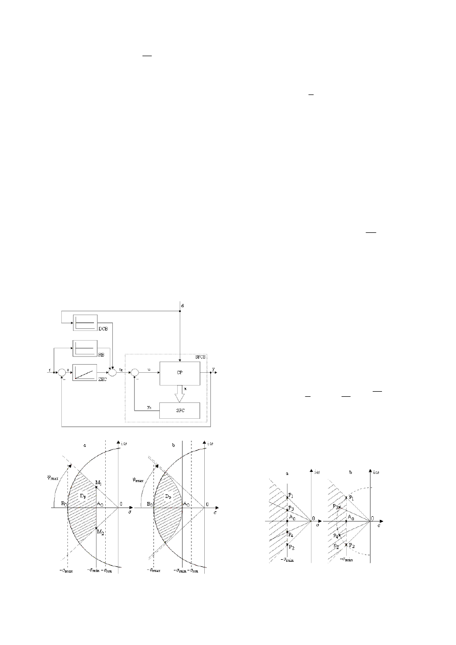
The classical SFCS structure extended with zero error

controller (ZEC), reference block (RB) and disturbance

compensation block (DCB) is presented in Fig. 1 (with CP

– controlled plant). The general principles concerning pole

placement designs applied to SFCSs are well known:
-

Due to the stability conditions, the poles must be

placed in the left-hand half-plane

0

}

Re{

<

s

keeping

a stability margin delimited by

sm

σ

−

.

-

The pole placement must ensure as small as possible

settling times in system’s transients. This leads to the

necessity for the absolute value of the real part of all

1-4244-2407-8/08/$20.00 ©2008 IEEE

Authorized licensed use limited to: Biblioteka Glowna i OINT. Downloaded on May 20, 2009 at 05:51 from IEEE Xplore. Restrictions apply.

poles (

n

k

i

p

k

k

k

,

1

,

=

ω

+

σ

=

with

n

– system’s

order),

|

|

|

}

Re{

|

k

k

p

σ

=

, to be as big as possible, and

|

|

|

|

}

Im{

k

k

k

p

σ

≤

ω

=

. The last requirement can be

expressed under the form of the condition

|

|

|

|

max

σ

<

σ

k

.

-

The choice of an extremely big value of

|

|

max

σ

implies difficulties to be avoided: big values of the

SFC gains, increased sensitivity with respect to

disturbance inputs, additional power at the actuator

level, etc.

Because of these motives, the literature does not offer

ideal or univocal recommendations on the pole placement.

In addition, the recommendations become less and less

accurate when the system order increases.

The above mentioned principles are expressed in terms

of the recommended domain of feasible poles D

p

illustrated in Fig. 2 in two versions, a and B. The version a

presented in Fig. 2 a is used frequently. The limitations

imposed through the values of

min

σ ,

max

σ and

max

ψ

depend on the maximum imposed settling time, the

overshoot

1

σ and the damping factor specific to the

transients, ρ and the constraints related to the

implementation of the SFC. One usual relationship is

)

3

(

2

/

min

max

>

σ

σ

, (1)

Fig. 1. Extended structure of state feedback control system

Fig. 2. Two versions of the domain of feasible poles

and the minimum value

min

σ is correlated often with the

following sum:

¦

=

ν

ν

≤

σ

n

p

n

1

min

|

}

Re{

|

1

. (2)

The value of

M

ψ is usually about 45

o

. The maximum

value,

max

σ , is fixed arbitrarily but in correlation with the

constraints related to the implementation of the SFC.

The first placement rule, which is common to many

methods, involves the hard constraint on the position of

two dominant poles p

1

and p

2

corresponding to the points

M

1

and M

2

in Fig. 2 a. The rule involves also the soft

constraint on the positions of the other poles p

3

, p

4

, etc. in

the domain D

p

. The classical methods of pole placement

concern the placement of the remaining (n–2) poles, they

are presented as follows and referred to as I to IV.

I. All poles fulfill the placement condition

n

p

p

,

3

,

}

Re{

}

Re{

min

2

,

1

=

ν

σ

−

=

=

ν

. (3)

The poles are placed on a parallel line to the imaginary

axis according to Fig. 3 a.

II. The poles are placed on a circle of radius

0

ω

centered in the origin. The circle contains the poles p

1

and

p

2

poles. The angle between two consecutives poles is

constant (Fig. 3 b).

Both methods are easy to use, but II ensures smaller

settling time. The performance of the SFCSs designed by

the methods I and II are satisfactory, but the settling time

takes generally big values.

III. The Butterworth configuration corresponds to the

poles of Butterworth filters. This method is recommended

when the CP and the SFCS do not have dominant zeros.

The placement condition is

n

n

n

i

p

,

1

]},

2

)

1

2

(

2

[

exp{

0

=

ν

π

−

+

π

ω

=

ν

. (4)

The method places the poles on a on a circle of radius

0

ω centered in the origin according to Fig. 4. For n>2 the

placed poles drop outside the recommended domain so the

system becomes more and more oscillating. Three

possibilities of pole placements can be used. They

correspond to three Butterworth circles:

Fig. 3. Poles with constant real part (a) and placed on a circle (b)

Authorized licensed use limited to: Biblioteka Glowna i OINT. Downloaded on May 20, 2009 at 05:51 from IEEE Xplore. Restrictions apply.

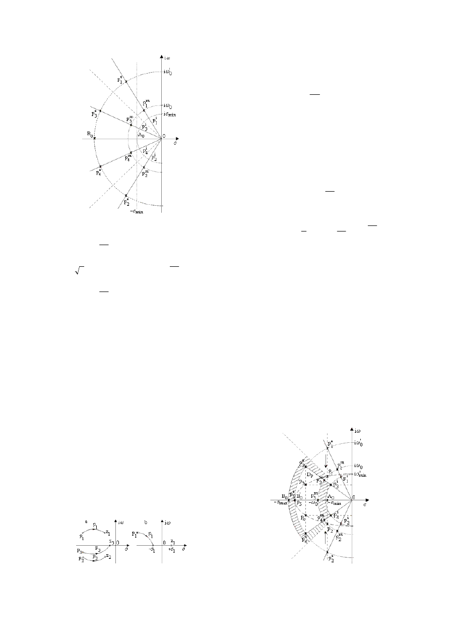
Fig. 4. Butterworth configurations

-

the internal Butterworth circle of radius

min

σ with the

poles

n

p

i

,

1

,

=

ν

ν

, resulting in the slowest SFCS,

-

the medium Butterworth circle of radius

min

0

2

σ

=

ω

with the poles

n

p

m

,

1

,

=

ν

ν

,

-

the external Butterworth circle of radius

'
0

ω with the

poles

n

p

e

,

1

,

=

ν

ν

, resulting in the fastest SFCS.

Only the settling times differ for the three previously

presented versions. The larger the system order is the

larger the overshoot will be.

IV. The minimization of the ITAE performance

criterion [11]

³

∞

=

0

d

|

)

(

|

t

t

e

t

I

, (5)

sets indirectly the pole placement. The calculation of the

integral becomes complicated for n >10.

V. If the controlled plant contains zeros, they will be

preserved in the SFCS structure that will exhibit more and

more oscillating transients as the zeros become more

dominant. That is the reason why it is advised to place the

poles such that they cancel the zeros as follows:

-

zeros placed in the left-hand half-plane are canceled

by poles taking the same values (Fig. 5 a),

-

zeros placed in the right-hand half-plane are canceled

by poles placed symmetrically on the imaginary axis

(Fig. 5 b).

If the cancellation process is imperfect, its favorable effect

will be lost. This is important when the zeros are close to

the imaginary axis.

Fig. 5. Pole-zero cancellation

III.

E

LLIPSE

-

BASED

P

OLE

P

LACEMENT

M

ETHOD

The idea behind this new method is to impose rigidly

that the two dominant poles p

1

and p

2

to be placed in the

points M

1

and M

2

(Fig. 2 a) with

min

2

,

1

}

Re{

σ

−

=

p

and

the other poles

n

p

,

3

,

=

ν

ν

, are placed on an ellipse

centered in the origin and passing through the points M

1

,

M

2

and B

0

(Fig. 2). The coordinates of the imposed poles

are illustrated in Fig. 6 (the domain D

p

is inside the dashed

region) and calculated according to the following steps:
-

Step 1. The values of

min

σ and

max

σ are set

accounting for the desired control system

performance indices and the constraints related to the

implementation of the SFC. Next the values of

0

ω

and

'
0

ω are determined.

-

Step 2. The poles

n

p

e

,

1

,

=

ν

ν

, are placed making use

of the external Butterworth configuration

n

n

n

i

p

e

,

1

]},

2

)

1

2

(

2

[

exp{

'
0

=

ν

π

−

+

π

ω

=

ν

. (6)

The first two poles must fulfill the condition

min

2

,

1

}

Re{

σ

−

=

p

. (7)

-

Step 3. Two situations arise depending on the position
of the point

)

0

,

(

'
0

'

0

i

B

ω

−

with respect to the point

)

0

,

(

max

0

i

B

σ

−

indicating the fastest Butterworth

filter. Firstly, if

'

0

B is placed on the right-hand side of

0

B , then no correction is needed. Secondly, if

'

0

B is

placed on the left-hand side of

0

B , then it will be

necessary to analyze whether the designed solution

fulfills the performance indices and constraints. If
not, then the position of

'

0

B will be position is

bounded to

0

B and a compromise to the value of

min

σ will needed possibly by approach to the origin.

Hence the control system becomes slower and the

abscissa of those poles will set the abscissa of the new

poles placed on the ellipse.

Fig. 6. Ellipse-based pole placement

Authorized licensed use limited to: Biblioteka Glowna i OINT. Downloaded on May 20, 2009 at 05:51 from IEEE Xplore. Restrictions apply.

-

Step 4. The poles

n

p

i

,

1

,

=

ν

ν

, are placed on the

internal Butterworth circle

n

n

n

i

p

i

,

1

]},

2

)

1

2

(

2

[

exp{

'
min

=

ν

π

−

+

π

σ

=

ν

, (7)

where the radius

'
min

σ is calculated in (8):

2

/

2

)

2

2

sin(

0

'
min

ω

=

π

+

π

σ

n

, (8)

for

1

=

ν

and

o

45

max

=

ψ

. These ordinate of these

poles will fix the ordinate of the new poles placed on

the ellipse.

-

Step 5. The dominant poles

p

1

and

p

2

are imposed to

be placed in the points

M

1

and

M

2

belonging to the

medium Butterworth circle of radius

min

0

2

σ

=

ω

for

o

45

max

=

ψ

but moved away from the poles

n

p

m

,

1

,

=

ν

ν

.

-

Step 6. Making use of (8), the

n

poles will be placed

on an ellipse centered in the origin and passing
through the points

M

1

,

M

2

and

'

0

B

:

.

,

,

1

),

2

2

sin(

)

2

2

cos(

'
0

'
min

'
min

'
0

ω

<

σ

=

ν

π

+

π

σ

+

π

+

π

ω

=

ν

n

n

i

n

p

(9)

The equation of that ellipse is

1

)

/

(

)

/

(

2

'
min

2

'
0

=

σ

ω

+

ω

σ

. (10)

It may degenerate to a circle under certain conditions.

IV.

P

OLE

P

LACEMENT

M

ETHOD

B

ASED ON

F

UZZY

L

INEAR

E

QUATIONS

Ackermann’s formula can be employed easily in case of

SISO linear systems resulting in the SFC gain matrix

k

T

:

)

(

]

1

...

0

0

[

1

A

S

k

P

T

−

−

=

, (11)

where

S

is the controllability matrix, with its well

accepted expression.

]

...

[

1

b

A

b

A

b

S

−

−

=

n

. The

matrix polynomial term

)

(

A

P

is obtained from the

desired characteristic polynomial of the closed-loop

system (the SFCS) calculated from the imposed poles

n

p

,

1

,

=

ν

ν

:

∏

=

ν

ν

−

=

n

p

s

s

P

1

)

(

)

(

. (12)

In uncertain environments, the crisp equation obtained

from the transformation of (11):

]

1

...

0

0

[

)

(

1

−

=

−

S

A

k

P

T

, (13)

can be viewed as a fuzzy equation. Unlike crisp equations,

which imply the identity of the left and right-hand

expressions, fuzzy equations do not necessarily carry this

implication. Several definitions of fuzzy equations are

given in [12] accepting the fuzzy sets A, B on R, a real

crisp variable x, and considering * an operator satisfying

Zadeh’s extension principle. Two such definitions are:

-

A type-Į equation is defined as A*x=B; the equation

means that the fuzzy set A*x is the same as the fuzzy

set B.

-

A type-Ȗ equation is defined as A*x§B; this definition

is one of the weak equalities and it is interpreted as

B

x

A

∈

=

*

if

≥∈

)

.

*

(

B

x

A

S

, where S is some scalar

measure of the similarity between two fuzzy sets and

∈

is a suitable threshold value.

In case of fuzzy numbers, a fuzzy linear equation is in

form of

B

x

A

~

~

~

=

, where A

~

, B

~

and x~ are fuzzy numbers.

It is well know that there exist no inverse numbers under

fuzzy numbers arithmetic addition and multiplication

respectively.

If F is a mathematical function involving fuzzy

parameters, then a number X can not be found generally

such that F(X)=B. Even if a solution does exist it becomes

difficult to find. A procedure to determine the degree to

which a proposed solution satisfies a given equation to

settle for a solution which only makes the given equation

only approximately true has been suggested in [13].

Large applicability in control systems can be found for

matrix equations

b

x

A

~

~

~

=

where

1

]

~

[

~

×

=

n

j

x

x

,

n

n

ij

a

×

=

]

~

[

~

A

is a matrix with fuzzy numbers as entries and

1

]

~

[

~

×

=

n

i

b

b

is a vector of fuzzy numbers. Differently expressed, the

fuzzy linear equation is

n

i

b

x

a

i

n

j

j

ij

,

1

,

~

~

~

1

=

=

¦

=

. (14)

Systems of linear interval equations are obtained taking

the Į-levels of (14). But these interval equations are hard

to solve, consequently the exact solution does not always

exists, and a first solution has been proposed in [14]. The

idea of this paper is to consider the equations (13) in the

framework of (14) accounting for the fuzzy modeling of

the controlled plant and the fuzzy pole placement.

V. C

ASE

S

TUDIES

The following six versions of pole placement methods

have been considered for third, fourth and fourth order

linear SFCSs: poles placed on the medium Butterworth

circle (B-m), poles placed on the external Butterworth

circle (B-e), poles resulted from the minimization of the

ITAE performance criterion (abbreviated by ITAE), poles

placed on a parallel line to the imaginary axis in terms of
the method I (M-I), poles placed on a circle of radius

0

ω

centered in the origin in terms of the method II (M-II), and

poles placed in terms of the ellipse-based pole placement

method presented in Section III (abbreviated EBPP). For
all six versions it is accepted that

'

0

B is placed on the

right-hand side of

0

B and

22

.

3

/

1

'
0

max

≤

ω

σ

≤

. The pole

configurations are calculated and presented in Table I

corresponding to all six pole placement versions.

Authorized licensed use limited to: Biblioteka Glowna i OINT. Downloaded on May 20, 2009 at 05:51 from IEEE Xplore. Restrictions apply.

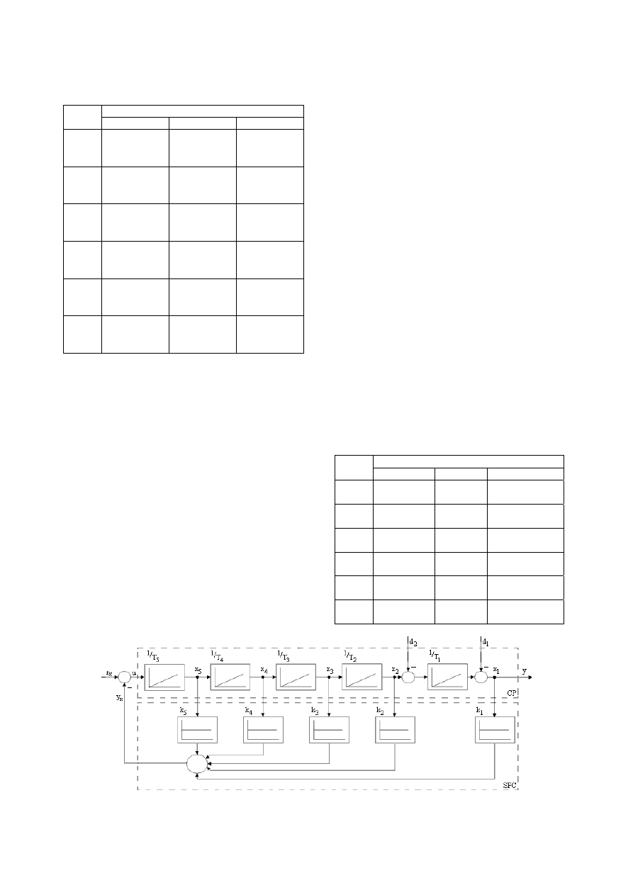
TABLE I.

P

OLE

C

ONFIGURATIONS

Method Case

study

n=3

n=4

n=5

B-m

–0.5

±0.866i,

–1

–0.3827

±0.924i,

–0.924

±0.3827i

–0.309

±0.5877i,

–0.809

±0.951i,

–1

B-e

–0.707

±1.2247i,

–1.4142

–0.707

±1.707i,

–1.707

±0.707i

–0.707

±2.176i,

–1.851

±1.345i,

–2.288

ITAE

–0.521

±1.068i,

–0.707

–0.424

±1.263i,

–0.626

±0.414i

–0.3764

±1.292i,

–0.575

±0.534i,

–0.8955

M-I

–0.707

±0.707i,

–0.707

–0.707

±0.707i,

–0.707

±0.3824i

–0.707

±0.707i,

–0.707

±0.293i,

–0.707

M-II

–0.707

±0.707i,

–1

–0.707

±0.707i,

–0.966

±0.2588i

–0.707

±0.707i,

–0.924

±0.3824i,
–1

EBPP

–0.707

±0.707i,

–1.4142

–0.707

±0.707i,

–0.707

±0.292i

–0.707

±0.707i,

–1.851

±0.437i,

–2.288

The controlled plant is characterized by the following

transfer functions [9]:

.

s

1

.

0

,

s

166

.

0

,

s

25

.

0

,

s

5

.

0

,

s

1

),

/

1

)(

/

1

)(

/

1

)(

/

1

)(

/

1

(

)

(

s,

1

.

0

,

s

25

.

0

,

s

5

.

0

,

s

1

),

/

1

)(

/

1

)(

/

1

)(

/

1

(

)

(

,

s

1

.

0

,

s

5

.

0

,

s

1

),

/

1

)(

/

1

)(

/

1

(

)

(

5

4

3

2

1

5

4

3

2

1

4

3

2

1

4

3

2

1

3

2

1

3

2

1

=

=

=

=

=

=

=

=

=

=

=

=

=

=

=

T

T

T

T

T

s

T

s

T

s

T

s

T

s

T

s

P

T

T

T

T

s

T

s

T

s

T

s

T

s

P

T

T

T

s

T

s

T

s

T

s

P

(15)

The SFCS structure is presented in Fig. 7, where d

1

and d

2

are disturbance inputs. The application of Ackermann’s

formula (11) for the three case studies gives the SFC

matrices presented in Table II.

The behaviors of the designed SFCSs can be analyzed

considering the effects in the system response with respect

to the modification of the reference input, the disturbance

input. The behavior in the frequency domain can be

analyzed, too [9]. The parametric modifications of the

controlled plant can be analyzed in both the frequency and

the time domain in terms of the sensitivity analysis and

eventually the robustness one.

Only the system behavior with respect to the unit step

modification of the reference input is presented here. With

this regard the several linguistic terms corresponding to

the performance indices defined in the time variation of

the controlled output are defined:

-

definitions for the overshoot

1

σ : VG (very good) for

%

7

%

0

1

<

σ

≤

, G (good) for

%

11

%

7

1

<

σ

≤

, A

(acceptable) for

%

15

%

11

1

<

σ

≤

, AQ (acceptable

but questionable) for

%

15

1

≥

σ

,

-

definitions for the first settling time

1

t : VG for

s

05

.

0

s

0

1

<

≤ t

, G for

s

07

.

0

s

05

.

0

1

<

≤ t

, A for

s

1

.

0

s

07

.

0

1

<

≤ t

, AQ for

s

1

.

0

1

≥

t

,

-

definitions for the settling time

s

t : VG for

s

08

.

0

s

0

<

≤

s

t

, G for

s

12

.

0

s

08

.

0

<

≤

s

t

, A for

s

15

.

0

s

12

.

0

<

≤

s

t

, AQ for

s

15

.

0

≥

s

t

,

-

definitions for the IAE performance criterion

³

∞

=

0

d

|

)

(

|

t

t

e

J

: VG for

5

.

0

0

<

≤ J

, G for

1

5

.

0

<

≤ J

, A for

5

.

1

1

<

≤ J

, AQ for

5

.

1

≥

J

.

Therefore the behavior of the fifth order system case study

in (15) with respect to the reference input is highlighted in

Table III.

TABLE II.

S

TATE

F

EEDBACK

C

ONTROLLER

M

ATRICES

Method Case

study

n=3

n=4

n=5

B-m

[.05 .1 .2]

[.13 .0334

.0865 .263]

[.0021 .0067

.0218 .0072 .324]

B-e

[.14 .2 .203]

[.013 .206

.291 .403]

[.131 .105

.261 .457 .74]

ITAE

[.05 .107

.175]

[.012 .0327

.0833 .21]

[.0021 .0071

.0229 .0833 .28]

M-I

[.035 .1 .212]

[.007 .027
.008 .203]

[.0009 .0045

.02 .0931 .354]

M-II

[.05 .107

.241]

[.0125 .042

.118 .335]

[.0021 .009

.033 .1312 .426]

EBPP [.707

.15

.283]

[.037 .096

.221 .4828]

[.0172 .0496

.131 .3593 .74]

Fig. 7. State feedback control system used in case studies

Authorized licensed use limited to: Biblioteka Glowna i OINT. Downloaded on May 20, 2009 at 05:51 from IEEE Xplore. Restrictions apply.

TABLE III.

P

ERFORMANCE

I

NDICES OF

F

IFTH

O

RDER

S

YSTEM

C

ASE

S

TUDY

(15)

IN

U

NIT

S

TEP

M

ODIFICATION OF

R

EFERENCE

I

NPUT

Method Performance

index

ı

1

t

1

t

s

J

B-m G VG A

VG

B-e G VG VG

AQ

ITAE G G VG

VG

M-I AQ AQ G VG

M-II AQ AQ A G

EBPP VG G

(VG) VG A

VI.

C

ONCLUSION

The ellipse-based pole placement method suggested

here for linear control systems exhibits the following

advantages with respect to other ellipse-based methods

reported in the literature:
-

The method does not require sophisticated either

reasoning and / or calculus.

-

The method ensures the univocal placement of poles

inside the recommended domain.

-

The dominant poles are placed in the very favorable

points M

1

and M

2

of the recommended domain that

ensures good SFCS performance indices

characterized by very good overshoot

(

%

5

%

4

1

≤

σ

≤

) and small settling time.

-

The real part of the remaining (n–2) poles is

increasing and their imaginary part is decreasing. This

results in fast and well damped SFCS transients.

-

The method is subject to easy implementation in

terms of algorithms and computer-aided design due to

its systematic six steps formulation.

However the single shortcoming, which is generally met

in all the other pole placement methods, is the rational
setting of

min

σ and

'
0

ω .

The pole placement method based on fuzzy linear

equations method proves to be easily understandable for

the designer and practitioner. Hence this original method

can be implemented in the framework of low-cost

automation solutions when the numerical problems

associated with it can be solved.

Both methods proposed here, the ellipse-based one and

the fuzzy linear equations-based one, can be extended to

the designs of state feedback observers by pole placement.

Extension to quasi-continuous digital control, digital

control, implementations, additional tests and applications

[15-20] represent directions of future research.

The linguistic characterization defined in the previous

Section allows the fuzzy characterization of system’s

behavior. This aspect leads to the idea of a new adaptive

fuzzy control system to be tackled in the future research.

A

CKNOWLEDGMENT

This work was supported by the cooperation between

Budapest Tech Polytechnical Institution and “Politehnica”
University of Timisoara (PUT), and University of
Ljubljana and PUT, in the framework of the Hungarian-
Romanian and Slovenian-Romanian Inter-governmental S

& T Cooperation Programs. The support from the
CNCSIS and CNMP of Romania is acknowledged. The
contribution of Mrs. Dipl. Ing. Angela Porumb in the early
phase of this project is appreciated.

R

EFERENCES

[1] B. C. Kuo and F. Golnaraghi, Automatic Control Systems, 8

th

Edition. New York: John Wiley & Sons, 2002.

[2] J. Ackermann, “Entwurf durch Polvorgabe,” Regelungstechnik,

vol. 25, pp. 173–179, April 1977.

[3] H. -R. Buehler, “Minimierung der Norm des Rückführvektors bei

der Polvorgabe,” Automatisierungstechnik, vol. 34, pp. 152–155,

April 1986.

[4] U. Konigorski, “Entwurf robuster, strukturbeschränkter

Zustandsregelungen durch Polgebietsvorgabe mittels
Straffunktionen,” Automatisierungstechnik, vol. 35, pp. 457–463,

Sept. 1987.

[5] W. Assawinchaichote and S. K. Nguang, “Fuzzy H

∞

output

feedback control design for singularly perturbed systems with pole
placement constraints: an LMI approach,” IEEE Trans. Fuzzy

Syst., vol. 14, pp. 361–371, June 2006.

[6] Y. G. Sun, L. Wang, G. Xie, and M. Yu, “Improved overshoot

estimation in pole placements and its application in observer-based
stabilization for switched systems,” IEEE Trans. Autom. Control,

vol. 51, pp. 1962–1966, Dec. 2006.

[7] Y. Kaiyang and R. Orsi, “Static output feedback pole placement

via a trust region approach,” IEEE Trans. Autom. Control, vol. 52,

pp. 2146–2150, Nov. 2007.

[8] U. Helmke, J. Rosenthal, and X. Wang, “Pole placement results

for complex symmetric and Hamiltonian transfer functions,” in
Proc. 46

th

IEEE Conference on Decision and Control, New

Orleans, LA, 2007, pp. 3450–3453.

[9] S. Preitl and A. Porumb, “About poles placement for sate feedback

control systems design,” in Proc. First International Conference
on Technical Informatics CONTI’94, Timisoara, Romania, 1994,

vol. 3, pp. 119–128.

[10] F. Liu, “Fuzzy pole placement design with H

∞

disturbance

attenuation for uncertain nonlinear systems,” in Proc. 2003 IEEE
Conference on Control Applications, Istanbul, Turkey, 2003, vol.

1, pp. 392–396.

[11] R. C. Dorf and R. H. Bishop, Modern Control Systems, 9

th

Edition.

Upple Saddle River, NJ: Prentice-Hall, 2007.

[12] D. Dubois and H. Prade, Fuzzy Sets and Systems: Theory and

Applications. New York: Academic Press, 1980.

[13] D. P. Filev and R. Yager, “Operations on fuzzy numbers via fuzzy

reasoning,” Fuzzy Sets and Systems, vol. 91, pp 137–142, Oct.

1997.

[14] J. Buckley and Y. Qu, “Solving systems of linear fuzzy

equations,” Fuzzy sets and Systems, vol. 43, pp 33–43, Sept. 1991.

[15] K. Tanaka, T. Ikeda, and H. O. Wang, “Fuzzy regulators and

fuzzy observers: relaxed stability conditions and LMI-based

designs,” IEEE Trans. Fuzzy Syst., vol. 6, pp. 250–265, May 1998.

[16] L. Horváth and I. J. Rudas, Modeling and Problem Solving

Methods for Engineers. Burlington, MA: Academic Press,

Elsevier, 2004.

[17] A. Sala, T. M. Guerra, and R. Babuška, “Perspectives of fuzzy

systems and control,” Fuzzy Sets and Systems, vol. 156, pp. 432–

444, Dec. 2005.

[18] I. Skrjanc, S. Blazic, and O. Agamennoni, “Interval fuzzy model

identification using l

∞

-norm,” IEEE Trans. Fuzzy Syst., vol. 13,

pp. 561–568, Dec. 2005.

[19] T. Orlowska-Kowalska and K. Szabat, “Control of the drive

system with stiff and elastic couplings using adaptive neuro-fuzzy
approach,” IEEE Trans. Ind. Electron., vol. 54, pp. 228–240, Feb.

2007.

[20] R. -E. Precup, S. Preitl, and P. Korondi, “Fuzzy controllers with

maximum sensitivity for servosystems,” IEEE Trans. Ind.

Electron., vol. 54, pp. 1298–1310, June 2007.

Authorized licensed use limited to: Biblioteka Glowna i OINT. Downloaded on May 20, 2009 at 05:51 from IEEE Xplore. Restrictions apply.