1

Monitoring and Early Warning

for Internet Worms

Cliff C. Zou

∗

, Lixin Gao

∗

, Weibo Gong

∗

, Don Towsley

†

∗

Department of Electrical & Computer Engineering

†

Department of Computer Science

Univ. Massachusetts, Amherst

Technical Report: TR-CSE-03-01

Abstract

After the Code Red incident in 2001 and the recent SQL worm in January 2003, it is clear that a

simple self-propagating worm can quickly spread across the Internet and infect most vulnerable computers
before people can take effective countermeasures. The fast spreading nature of these worms calls for
a worm monitoring and warning system. In this paper we propose an effective early warning system.
Based on epidemic models and observation data of a fast-spreading worm, we deploy a Kalman filter
to predict worm propagation in real-time. Furthermore, we can effectively correct the bias introduced
by the observed number of infected hosts. Our simulation results for the Code Red and SQL worm
show that with observation data from a small fraction of IP addresses, we can accurately predict the
worm infection rate when the worm infect about 5% of all vulnerable computers. The total number of
vulnerable computers can also be estimated quickly.

I. I

NTRODUCTION

Since the Morris worm in 1988 [16], the security threat posed by worms has steadily increased,

especially in the last several years. In 2001, the Code Red and Nimda worms infected hundreds of
thousands of computers [13][17], causing millions of dollars loss to our society [9]. These two worms
demonstrated how vulnerable our computer networks are when facing an actively propagating worm.
Furthermore, Staniford et. al presented some worm design techniques such that the new worm could
spread even faster [19]. After a relatively quiet time, the SQL worm recently appeared on January 25th
2003 and quickly spread throughout the Internet. Because its vulnerable population was much smaller
than what Code Red and Nimda had, and also because it was much easier to block the SQL worm traffic
than to block Code Red and Nimda, the SQL worm was quickly constrained after one day [20][15].
However, the SQL worm used UDP to send scans. Thus, while it was active, it sent out huge amount
of scan packets and formed a denial of service attack. Many networks across Asia, Europe and America
were shut down for several hours [6].

Currently, some organizations and security companies, such as the CERT, CAIDA, and SANS Institute

[4][2][18], are monitoring the Internet and paying close attention to any abnormal traffic. Nevertheless,
there is no nation-scale malware monitoring and defense center. Given the fast spreading nature of the
Internet worms, it seems appropriate to setup a worm monitoring and early warning system. In addition,
by collecting more complete data on the worm propagation via the monitoring system, we could estimate
and predict a worm propagation trend and its behavior at its early stage for automatic mitigation.

2

In this paper, we mainly focus on worms that uniformly scan the Internet. The most widespread Internet

worms, including both the Code Red worm and the recent SQL worm, belong to this category. Uniform
scan is a simple and efficient way for worm to propagate when the worm has no knowledge of where
vulnerable computers reside. In fact, more “sophisticated” worms that try to exploit such knowledge
still require certain forms of uniform scanning. For example, a prior knowledge “hitlist” can dramatically
increase worm spreading speed [19]. However once the victims on the hitlist are infected, a worm will still
need to launch a uniform scan from the initial victims. [21] proposed “permutation” technique to improve
worm spreading speed, but it still involve local random scan. Code Red II [8] used local preference in
selecting target IP address. However, local preference scanning might slow down the worm propagation
[5]. In fact, local scans can also cause considerable traffic within local networks that can slow down the
worm scan rate to outside world. In fact, if we can uniformly or regularly distribute the monitors over
the unused IP address space with appropriate density, we should be able to extend our work reported
here to cover these cases.

We believe early warning for fast spreading worms is possible for the following reasons. First, at the

initial stage of propagation there is little human intervention and the worm propagation can be modelled
quite accurately [19]. Second, even though we try to obtain good estimates for worm propagation in a
very short time, the port scan observations are still statistically significant due to the scale and speed of
the Internet worms. Third, the deployment of an effective worm monitoring system to collect port scan
observations is not expensive. Our simulation study indicates that with about one million IP addresses
monitored we can accurately estimate the worm propagation speed when less than 5% of the susceptible
population is infected. The total number of vulnerable machines can also be estimated when about 10%
to 15% of the susceptible population is infected. We believe these estimates are good enough to provide
an early warning that could be used to trigger a system administrator’s action, automatic port blocking
or other containment mechanisms such as those evaluated in [14].

The rest of this paper is organized as follows. Section II gives a brief introduction of the worm model

used in this paper. In Section III, we propose the architecture of the worm monitoring system. In Section
IV, we describe the type of data that should be collected by the monitors and how to correct for biases
within the observation data. In Section V, we present effective algorithms to estimate worm infection
rate and the susceptible population for early warning. We discuss future work in setting up the worm
monitoring and early warning system in Section VI. Section VII is the conclusion.

II. W

ORM

P

ROPAGATION

M

ODEL

A promising approach for modelling and evaluating the behavior of malware is the use of fluid models.

Fluid models are appropriate for systems that consists of a large number of vulnerable hosts involved in
a malware attack. A classic model, taken from modelling the spread of epidemics, assumes that each host
resides in one of two states: susceptible or infectious. The model further assumes that, once infected by
a virus or worm, a host remains in the infectious state forever. Thus only one state transition is allowed
by each host: susceptible

→ infectious [11]. The classical simple epidemic model for a finite population

is

dI

t

dt

= βI

t

[N − I

t

],

(1)

where

I

t

is the number of infected hosts at time

t; N is the size of population; and β is referred to as

the pairwise rate of infection in classical epidemic studies [10]. At

t = 0, I

0

hosts are infectious while

the remaining

N − I

0

hosts are susceptible. This model could capture the mechanism of a uniform scan

worm, especially for the initial part of the worm propagation [19].

3

TABLE I

N

OTATIONS IN THIS PAPER

Notation

Definition

N

Total number of hosts under consideration

I

t

Number of infected hosts at time

t

∆

The length of monitoring interval (time unit in discrete-time model)

β

Pairwise rate of infection in epidemic model

α

Infection rate per infected host,

α = βN

C

t

Number of infected hosts monitored by time

t

Z

t

Monitored worm scan rate at time

t

η

Scan rate per infected host

p

Probability a worm scan is monitored

y

t

Measurement data in Kalman filter

δ

Constant in measurement equation

y

t

= δI

t

+ w

t

R

Variance of observation error

MWC

Abbreviation for “Malware Warning Center”

0

100

200

300

400

500

600

0

0.5

1

1.5

2

2.5

3

3.5

4

4.5

5

x 10

5

Time t

Slow spreading
phase

Fast spreading phase

Slow finishing
phase

Fig. 1.

Worm propagation model

Fig. 1 shows the dynamics of

I

t

as time goes on for one set of parameters. From this figure, we observe

that we can roughly partition the worm propagation into three phases: the slow spreading phase, the fast
spreading phase, and the slow finishing phase. During slow spreading phase, the number of infected hosts
increases slowly. During this phase since

I

t

N, the number of infected hosts increases exponentially

according to model (1). After a certain number of hosts are infected and participate into infecting others,
the worm enters the fast spreading phase where vulnerable hosts are infected at a fast speed. When most
of vulnerable computers have been infected, the worm enters the slow finishing phase because the few
vulnerable computers left are very hard for the worm to search out. Our task is to provide an accurate
estimate of the worm’s “natural” spreading rate based on observations during the slow spreading phase.

In this paper we will model the worm propagation as a discrete-time system. The time will be divided

into monitoring interval of length

∆. To simplify the notations, we use “t” as a discrete time index. The

real time interval between

t − 1 and t is ∆. From (1), the discrete-time epidemic model can be written

4

as:

I

t

= I

t−1

+ βNI

t−1

− βI

2

t−1

= (1 + α)I

t−1

− βI

2

t−1

(2)

where

α = βN . We call α the infection rate, the average number of vulnerable hosts that can be infected

per

∆ time by one infected host during the early stage of worm propagation.

Table. I lists most of the notations used in this paper. We use the notation ˆ

I

t

to denote the estimated

value of

I

t

.

Before we go on to discuss how to use the worm model (2) to estimate and predict worm propagation,

we will first present the monitoring system design in the next Section III and data collection issues in
Section IV.

III. M

ONITORING

S

YSTEM

In this section, we propose an architecture for a worm monitoring system. The monitoring system

aims to provide early warning for worm activities by estimating its potential propagation. The monitoring
system consists of a Malware Warning Center (MWC) and distributed monitors as shown in Figure 2.
The monitors gather data on worm scan activities and send the data to the Malware Warning Center. The
data sent out by the monitors can be either raw scan data or results from preliminary processing of the
data by the monitors.

A. Monitoring System Architecture

Fig. 2.

A generic worm monitoring system

There are two kinds of monitors: egress scan monitors and ingress scan monitors. Ingress scan monitors

are distributed across the Internet and located on local gateways or routers on stub networks. The goal
of the ingress scan monitor is to monitor the scan traffic coming into a stub network by logging the
incoming traffic to unused IP addresses or unused port numbers. The local network administrators have
the best knowledge about how addresses or port numbers inside their networks are allocated. Therefore,
it’s easy for them to setup the ingress scan monitor at one or several routers in their stub networks.

The stub network can also be a black hole network that is set up solely for the purpose of receiving

scan packets. The black hole network does not have any physical machines but the address space covered
by it is announced globally. According to BGP routing tables, only about 30% of IP addresses have
been allocated. It is possible to register some unallocated blocks of IP addresses and place monitors on
these IP address blocks. As a result, a monitor can log scan traffic to an IP address block. Black hole

5

networks have been used for monitoring worm activities. For example, during the Code Red incident on
July 19th, 2002, a /8 network at UCSD and two /16 networks at Lawrence Berkeley Laboratory were
used to collect Code Red scan traffic. All port 80 TCP SYN packets to these networks were considered
to be Code Red scans [13].

Egress scan monitors are located at an egress point of a stub network. The goal of an egress scan

monitor is to monitor the outgoing traffic from a network to infer potential scan activities or scan rate of
a worm. The ingress scan monitors listen to the global traffic on the Internet and can monitor only the
traffic from the Internet. However, it is difficult to determine the behavior of each individual worm from
the data collected by these monitors because not all of the scans sent out by an infected host can be
captured by these monitors. Therefore, it is necessary for us to use egress scan monitors. If a computer
inside a local network is infected, the egress filter on this network can receive most of the scans sent out
by the compromised computer. The closer the egress scan monitor is to an infected computer, the more
complete the data that we can get on the worm’s scan behavior.

For real-time worm warning, the distributed monitors are required to send observation data to MWC

continuously without significant delay, even when the worm scan traffic has caused congestion to the
Internet. For this reason, we can set up a tree-like hierarchy of data mixers between monitors and the
MWC: the MWC is the root; the leaves of the tree are monitors (either ingress scan monitor or egress
scan monitor). Each data mixer is responsible for several nearby monitors. These monitors send observed
data to the data mixer. After fusing this data together, the data mixer passes the data to a higher level data
mixer. An example of fusion might be the removal of redundant addresses from the lists of addresses of
infected hosts reported to the data mixer.

In addition to egress and ingress scan monitors, we can also set up honeypots on unused IP addresses

(they are special ingress scan monitors). These honeypots can accept worm scans and receive the worm
payload. The worm code can be forwarded to the MWC, where it would be analyzed by security experts.

B. Location Selection for Distributed Monitors

For ingress scan monitors, it is ideal to cover as much address space as possible. In addition, we need

to ensure the quality of the address space. For example, it is not efficient to cover well-known reserved
address blocks since hackers can program a worm to avoid these address blocks. As another example,
we could use a large unallocated IP block for the ingress monitors. However, if our monitoring system
is known by the worm designers, they can easily remove this address block from their scanning scope.
Therefore, an important issue is the address space selection. The key to an effective monitoring strategy
is to overlap the address space covered by the monitoring system with the address space scanned by the
worm as much as possible. By uniformly distributing monitors, we can achieve an effective sample of
worm activities. Since worms might choose different destination addresses by using different preferences,
e.g., non-uniform scanning, we need to use multiple address blocks with different sizes and characteristics
to ensure proper coverage.

For egress scan monitors, the worm on different infected computer will exhibit different behaviors.

For example, the worm scan rate is constrained by the computer’s bandwidth. Therefore, we need to set
up multiple egress filters to record the scan behaviors of infected hosts at different locations. In addition,
these egress scan monitors should be scattered in order to cover different network environments.

C. Some Monitoring Principles

Distributing monitors across the Internet can help us distinguish a real spreading worm from hacking

activities. Hackers scan the Internet every day. For example, the Internet Storm Center of incidents.org
provides us the up-to-date reports on port scan activities on the Internet [12]. These scans will appear as

6

noise to our monitoring system. They are usually targeting some specific part of the Internet or scanning
many ports (e.g., for the purpose of collecting network information. On the other hand, a fast spreading
worm will spread through the entire Internet and generate the same type of scans everywhere. If most
of our distributed monitors discover a surge of a particular type of scan, we can have high confidence to
claim that a worm is spreading through the Internet.

In order to prevent hackers or worms from discovering the IP blocks covered by black hole monitors,

the monitors should reply to a sample of scans they receive. An ingress scan monitor can pre-generate
a list of IP addresses that it should reply for when scans arrive directed to these addresses. Since an
allocated IP space contains many unused IP addresses, the monitors should not reply to all received
scans. In addition, when the worm sends too many scans to a monitor, the monitor can stop responding
to worm scans just like an overwhelmed router or gateway. As a result, the ingress scan monitors will
not incur denied of service by the heavy worm traffic and at the same time behaves just like real local
networks.

Usually a worm appears long after the vulnerability has been discovered. For example, Code Red

worm appeared one month after the Windows IIS security hole was discovered [7]; the recent SQL worm
spread six months after the SQL server vulnerabilities were discovered [20]. Therefore, we can design
our monitoring system to have a priority list that includes previously discovered critical vulnerabilities
— all monitors should give high priority to record scans towards these vulnerabilities.

IV. D

ATA

C

OLLECTION AND

C

ORRECTION

After setting up the monitoring system, we need to determine what kind of data should be collected.

The main task for an egress scan monitor is to determine the behavior of individual worm inside its
network, such as the worm’s scan rate and scan distribution. Let us denote the scan rate as

η, namely

the average number of scans sent out by infected host per

∆ time. During each monitoring interval ∆,

an egress scan monitor records the number of infected hosts inside its network that send out scans and
also the number of scan attempts, and then passes these two numbers to the MWC, where such data is
collected from all egress scan monitors and used to calculate the average worm scan rate

η.

Both Code Red worm and SQL worm scanned the Internet IP address space uniformly [7][20]. However,

not all worms behave in such simple way, such as Code Red II [8], which exhibited a local preference
in selecting target IP address. Therefore, it’s important to use egress scan monitors to infer the worm
scan distribution; and the egress scan monitors should cover different sizes of networks in order to more
accurately infer the worm distribution.

To estimate and predict worm propagation in real-time, the ingress scan monitors are required to record

two types of data: the number of scan attempts they receive at

i-th monitoring interval, i = 1, 2, · · · ; and

the IP addresses of infected hosts that have sent scans to the monitors by time

∆i. Each time a monitor

sends an IP address list to the MWC, it only includes the IP addresses of those newly appeared infected
hosts since the last report.

If all monitors send observation data to the MWC every monitoring interval time, we can obtain the

following observation data at each discrete time epoch

t, t = 1, 2, · · · :

•

The worm scan distribution, e.g., uniform scan distribution or scan with address preference.

•

The worm scan rate

η.

•

The total number of scan attempts in a monitoring interval time from time

t − 1 to t, denoted by

Z

t

.

•

The number of infected hosts observed by time

t, denoted by C

t

.

It may be useful to record other types of data. For example, the time stamp of each scan may be useful

for statistical analysis. For the purpose of predicting worm propagation discussed in this paper, we only
need the previously described observation data.

7

A. Correction of biased observation data

In this paper, we primarily focus on worms that uniformly scan the Internet. Denote

p as the probability

that a worm scan is monitored by our monitoring system. If our monitors cover

m IP addresses, then

a worm scan has the probability

p = m/2

32

to hit our monitors. From the discrete time

t − 1 to t, in

average a worm sends out

η scans. Thus the total number of worm scans send out by all infected hosts

in this monitoring interval is

ηI

t

. Therefore, from the definition of

Z

t

, we have

E[Z

t

] = ηpI

t

.

(3)

It means that observation data

Z

t

is proportional to the real number of infected hosts on the Internet.

Each worm scan has a very small probability

p to hit our monitors. An infected host will send out

many scans before one of them is observed by our monitors (like a Bernoulli trial with small probability).
Therefore, the number of infected hosts monitored by time

t, is not proportional to the real number of

infected hosts at the current time

t (see the following experiment Fig. 3 and Fig. 4). In the following,

based on mean value analysis, we present an effective way to obtain an unbiased estimate for the number
of infected hosts

I

t

based on

C

t

and worm scan rate

η.

From our monitoring system, we can obtain the worm scan rate

η directly. Since we know how many IP

addresses our monitors covers, it’s easy to calculate the probability

p that a worm scan hits our monitors.

In a monitoring interval time, a worm sends out

η scans, thus the probability that an infected host has

sent at least one scan to our monitors is

1 − (1 − p)

η

.

At time

t − 1, suppose our monitoring system has observed C

t−1

infected hosts. At time

t, the number

of infected hosts that have not been observed by time

t − 1 is I

t

− C

t−1

. During the monitoring interval

from

t − 1 to t, each infected host has probability 1 − (1 − p)

η

to scan the monitors (at least one scan in

η hit the monitors). Thus the average number of infected hosts monitored at time t conditioned on C

t−1

is

E[C

t

|C

t−1

] = C

t−1

+ (I

t

− C

t−1

)[1 − (1 − p)

η

].

(4)

Remove the condition on

C

t−1

and we have

E[C

t

] = E[C

t−1

] + (I

t

− E[C

t−1

])[1 − (1 − p)

η

],

(5)

which means we can derive

I

t

from the average value of the observed data

E[C

t

] according to:

I

t

=

E[C

t

] − (1 − p)

η

E[C

t−1

]

1 − (1 − p)

η

(6)

Since

E[C

t

] is unknown, we use observed data C

t

to replace it and write the estimated value of

I

t

as

ˆI

t

=

C

t

− (1 − p)

η

C

t−1

1 − (1 − p)

η

(7)

Note that by using discrete-time model, we assume all newly infected hosts from discrete time

t − 1

to

t are infected immediately after the time epoch t − 1 ( i.e., they are infected right after time ∆(t − 1)

in the real world). Therefore, in order to derive the ˆ

I

t

accurately by (7), the monitoring interval should

be small enough compared with the worm scan rate.

In the following, we analyze how the observation error of

C

t

would affect the estimated value of

I

t

.

Suppose the observation data

C

t

is

C

t

= E[C

t

] + w

t

(8)

8

where the observation error

w

t

is a white noise with variance

R. Substituting (8) into bias correction (7)

and we have

ˆI

t

= I

t

+ µ

t

(9)

where error

µ

t

is

µ

t

=

w

t

− (1 − p)

η

w

t−1

1 − (1 − p)

η

(10)

Therefore, the estimated value ˆ

I

t

is unbiased since

E[µ

t

] = 0. The variance of the estimated error is

E[µ

2

t

] =

1 + (1 − p)

2η

[1 − (1 − p)

η

]

2

E[w

2

]

(11)

Because

p is a very small probability, (1 − p)

η

≈ 1 − ηp. Substitute it into the equation above and we

have the variance of the estimated error:

E[µ

2

t

] ≈

2(1 − ηp)

(ηp)

2

R

(12)

We can see that by using the bias correction (7), we amplify the observation error of

C

t

. The estimated

ˆI

t

would be more noisy than observed

C

t

. If our monitors cover less IP space,

p would decrease, then

(12) shows that the estimated ˆ

I

t

would be more noisy. Therefore, we have to let our monitors to cover

enough IP space in order to get accurate estimation on how many computers are infected.

We simulate Code Red to check the validity of (7). In the simulation, we assume there are

500, 000

vulnerable hosts on the Internet. Code Red sends out five scans per second choosing IP address randomly.
The monitoring system covers

2

17

IP addresses (equal to two Class B networks). The monitoring interval

is set to be one minute, thus the worm scan rate is

η = 5 × 60 = 300. Each scan has the probability

p = 2

17

/2

32

to hit the monitors. The simulation result is shown in Fig. 3.

0

100

200

300

400

500

600

700

800

0

0.5

1

1.5

2

2.5

3

3.5

4

4.5

5

x 10

5

Time t (minute)

Number of infected hosts

Real infected hosts
Observed infected hosts
After bias correction

Fig. 3.

Estimate

I

t

based on the biased observed

C

t

(Monitoring

2

17

IP space)

100

200

300

400

500

600

700

800

0

0.5

1

1.5

2

2.5

3

3.5

4

4.5

5

5.5

x 10

5

Time t (minute)

Number of infected hosts

Real infected hosts
Observed infected hosts
After bias correction

Fig. 4.

Estimate

I

t

based on the biased observed

C

t

(Monitoring

2

14

IP space)

Fig. 3 shows that the curve of the observed number of infected hosts,

C

t

, deviates substantially from the

curve of the real value

I

t

. After the bias correction by using (7), the number of estimated infected hosts

9

obtained from our monitors (with small noise) matches well with the real number of infected hosts in the
simulation. Because we simulate a large-scale worm spreading where the population is

N = 500, 000,

the worm propagation is almost a deterministic process. Therefore, the curves of

I

t

and

C

t

are smooth.

Moore et. al [13] collected such kind of data

C

t

during the Code Red propagation on July 19th, 2001.

We can see that the curve

C

t

in Fig. 3 is similar to the curve of the number of code red infected hosts

they observed on two Class B networks.

If our monitors only cover

2

14

IP addresses, then

p = 2

14

/2

32

and the simulation result is shown in

Fig. 4. We can see that the estimated ˆ

I

t

is too noisy because of the error amplification effect described

by (12).

V. E

STIMATION FOR

W

ORM

V

IRULENCE

How to mitigate malware, especially Internet worms such as the Code Red of 2001 and the SQL

worm of 2003, is a serious challenge to network security researchers. The monitoring system described
in the previous sections can provide us information about the worm spreading status. Worm spreading
is a dynamic process. The basic spreading mechanism in recent malware is to spread through random
scanning and reproduction. We need to estimate the spreading parameters for early warning. This is
possible since we have a large set of data from the monitoring system and a good model to represent the
spreading dynamics. The simple epidemic model (2) provides a good starting point for the development
of parameter estimators. In this section we propose estimation methods based on recursive filtering
algorithms for stochastic dynamic systems such as the Kalman filter (see, for example, [1]).

Our monitoring system can track a variety of port scans, their rates, and the sources of these scans. An

abnormal increase in scan rates can be used to trigger the prediction system described in this section to
provide an early warning signal. For this prediction, it is important to quickly obtain accurate estimates
for the malware spreading parameters. Thanks to the speed and scale of the worm spreading, a rich set of
information about the propagation behavior of worms is available in the initial stage of their spreading.
With the monitoring system presented in Section III, we can gather the necessary information to provide
early warning and prediction of the impact of the ongoing worms.

Assume that at MWC, we can collect the reports from the monitors continuously in real-time. Our

task, then, is to develop algorithms for estimating the spreading parameters. We focus on the simple
epidemic model described in equation (2).

A. Problem Description

As discussed before, in the initial phase, we expect worm propagation to be well described by the

simple epidemic model since there will be little mitigation effort and not much congestion caused by the
worm scans [23]. Moreover, for the worm to be effective, the propagation rate should be quite high (a
slow worm typically would not “make it” in the Internet due to phase transition effect [11]). We expect
this to provide a good signal to noise ratio for the purpose of estimating the propagation.

In the monitoring system, all monitors periodically report observation data, such as

C

t

or

Z

t

, to MWC

at each monitoring interval. At the MWC, we want to recursively estimate the parameters

β, N , and

α based on observation data. In the following, we will first provide a Kalman filter type algorithm to
estimate parameters

α and β.

Let

y

1

, y

2

, · · · , y

t

, be measurement data in the Kalman filter algorithm.

y

t

has a simple relationship

with the number of infected hosts

I

t

,

y

t

= δI

t

+ w

t

(13)

where

w

t

is the observation error.

δ is a constant ratio: if we use Z

t

as

y

t

, then

δ = ηp as shown in (3);

if we use ˆ

I

t

derived from

C

t

by the bias correction (7), then

δ = 1. We also assume that the observation

10

error

w

t

is a white noise with variance

R, where R decreases when our monitors cover larger IP address

space and provide more accurate observation data.

B. Parameter Estimation based on Kalman Filter

From (13), we have

I

t

= y

t

/δ − w

t

/δ

(14)

Substitute (14) into the worm model (2), we have the equation describing the relationship between

y

t

and worm’s parameters:

y

t

= (1 + α)y

t−1

−

β

δ

y

2

t−1

+ ν

t

(15)

where the noise is

ν

t

= w

t

− (1 + α)w

t−1

− β(w

2

t−1

− 2y

t−1

w

t−1

)/δ

(16)

and its mean value is

E[ν

t

] =

β

δ

E[w

2

t−1

] =

βR

δ

.

(17)

A recursive least square algorithm for

α and β can be cast in a standard Kalman filter format [1]. Let

ˆα

t

and ˆ

β

t

denote the estimated value of

α and β at time t, respectively. Define the system state vector

as

X

t

=

1 + α

−β/δ

. If we denote

H

t

= [ y

t−1

y

2

t−1

], then the system is described by:

X

t

= X

t−1

y

t

= H

t

X

t

+ ν

t

(18)

and the Kalman filter to estimate the system state

X

t

is














H

t

= [ y

t−1

y

2

t−1

]

K

t

= P

t−1

H

τ

t

/(H

t

P

t−1

H

τ

t

+ R

ν

)

P

t

= (I − K

t

H

t

)P

t−1

ˆ

X

t

= ˆ

X

t−1

+ K

t

(y

t

− H

t

ˆ

X

t−1

)

(19)

where

R

ν

is the variance of noise

ν

t

. When we don’t know

R

ν

, we can simply let it be

1. From the

experiments we found that the value of

R

ν

is not important.

For large-scale worm modeling,

β is very small, on the order 1/N . Thus the mean value of noise ν

t

described by (17) is negligible (for the worm modeling,

δ is neither too big nor too small). However,

ν

t

is a correlated noise. Thus the estimated value

ˆα and ˆβ derived from our Kalman filter may have a

small bias. In this paper, we try to estimate the parameter

ˆα with an acceptable bias error by using more

accurate observation data (the bias drops when the observation error

w

t

has smaller variance). The bias

can be eliminated by refining the algorithm to deal with the correlated noise

ν

t

. This will further reduce

the monitors needed.

If we use

Z

t

as the measurement

y

t

in the Kalman filter and do not know

δ, we still can estimate the

infection rate

α by letting δ = 1. The Kalman filter (19) doesn’t depend on δ; the value of δ only affects

the estimated value of

β.

11

C. Estimation of the Vulnerable Population

For a large-scale worm propagation, the parameter

β in model (2) is usually a very small number (it

is on the order of

1/N). In the Kalman filter above, the system state is X

t

= [ 1 + βN −β/δ ]. The

two elements in the state differ in the order of

N . Thus the Kalman filter can estimate the parameter α

accurately but is not good at estimating

β. Consequently the estimate of N using ˆ

α/ ˆ

β is not good.

We now present an effective way to estimate the population

N based on worm scan rate η and the

estimated

α from the Kalman filter above. A uniform scanning worm sends out η scans per monitoring

interval; each scan has probability

N/2

32

to hit one host in the population under consideration. Hence, at

the beginning when most hosts in the population are vulnerable, a worm can infect, on average,

ηN/2

32

hosts per monitoring interval (the probability of two scans hitting the same host is negligible). From the
definition of infection rate

α, we have α = ηN/2

32

. Therefore, the population

N is

N =

2

32

α

η

(20)

where the worm scan rate

η can be obtained directly from egress scan monitors in our monitoring system.

We can use this equation to estimate

N along with the Kalman filter in estimating α. In this way, the

estimate

N can have similar convergence properties to that of the estimate for α from the Kalman filter.

D. Issues on Using Observation Data to Estimate Worm Virulence

Here we discuss how we use observation data and algorithms above to estimate worm virulence.
From the egress scan monitors in the monitoring system, we can obtain the worm scan rate

η directly.

For the purpose of early warning and prediction, we need to estimate the worm parameters,

N , α and

β, as early as possible. We can either use C

t

, the number of observed infected hosts, or

Z

t

, the number

of scan attempts observed in a monitoring interval time. Here we believe that using scan attempts

Z

t

is

more appropriate than using the number of observed hosts

C

t

.

Based on observation

η and Z

t

, we can estimate all the parameters of the worm at each discrete time

in the following order:

•

Estimate the infection rate

ˆα from the Kalman filter (19).

•

Estimate the population ˆ

N from Equation (20) based on η and estimated ˆ

α.

•

Estimate ˆ

β by ˆ

β = ˆ

α/ ˆ

N .

When we use the estimation algorithms to estimate worm propagation, it’s impossible for us to use

them immediately after the worm begins to propagate from several infected hosts. At this time the worm’s
scan traffic is buried among normal scan activities. The MWC can’t determine that a worm is spreading
based on observation data, and the signal to noise ratio is too low. So when we implement these estimation
algorithms in the monitoring system, they are activated only when the MWC receives a hight number of
scans that is over a predetermined threshold. Therefore, in our simulation experiments, we begin to use
these recursive estimation algorithms after some time to simulate such activation delay.

As shown in [19], a worm that uses “hitlist” can dramatically increase its spreading speed if it first

infects all computers on the hitlist. However, our monitoring system and the estimation algorithms can
still deal with it as long as the worm use random scan after it infects computers on the hitlist. When the
worm begins to randomly scan to propagate, it has a large number of infected hosts that send scans out.
Therefore, our monitors will observe a sudden surge of scans and the MWC will immediately activate the
estimation algorithms. In addition, at this time the signal to noise ratio is high because of large amount
of scans. The estimation algorithms can quickly converge.

We prefer to use

Z

t

instead of

C

t

because of two reasons:

12

•

Additional noise is introduced if we use

C

t

.

•

Collecting

Z

t

from distributed monitors is more quick and robust than collecting

C

t

.

The first reason is that the

C

t

is biased as explained in Section III. We must first use (7) to correct the

bias of

C

t

. At the beginning, when the number of infected hosts are small, our egress scan monitors can

only observe few infected hosts sending out scans. Thus the observed average infection rate

η is noisy.

Using Equation (7) will bring in the additional noise of

η. On the other hand, we can use Z

t

directly

without introducing such kind of noise.

The second reason is about real-time data collection in the monitoring system. For the purpose of

prediction, we need each monitor to send data to the MWC in every monitoring interval. The monitoring
interval,

∆, is determined by the speed of the worm. For fast spreading worm such as the SQL worm,

we need to use 1 second as the monitoring interval in order to catch its speed as shown in the following
experiments. Therefore, we should let each monitor send out data as small as possible to the central
server, especially during the worm fast spreading period. For this reason, sending the single number

Z

t

each monitoring interval is very quick and robust to the possible congestion caused by the worm. On the
other hand, for the observation

C

t

, each monitor must send all the source IP addresses of scans that it

observes in a monitoring interval time to the MWC. This address list could be very long if the monitor
takes charge of a large IP space.

We prefer to use

Z

t

instead of

C

t

, but it doesn’t mean that the observation data

C

t

is not useful. The

curve of

Z

t

in ideal case should match with the curve of

C

t

after bias correction. Therefore, we can use

C

t

to double check if our observed data

Z

t

are correct. In addition, in the process of obtaining

C

t

, we

can know each of the source IP address of infected hosts that are monitored. This IP address list can
help Malware Warning Center to cooperate with other ISPs and take effective countermeasures.

For the observation data of

C

t

, the monitors can send the source IP addresses of infected hosts to the

MWC in a larger time interval, e.g., 10 times of the time interval used in sending

Z

t

.

E. Simulation Experiments

We simulate both Code Red in July 19th, 2001 [7] and the recent “SQL worm” on January 25th, 2003

[20]. In the case of Code Red worm, we set the total number of vulnerable computers on the Internet
at 500,000 and the scan rate at 5 scans per second with IP addresses chosen randomly. We set up a
monitoring system that occupies

2

20

IP space. The monitoring system can record all Code Red scan

attempts targeting their IP space (it doesn’t matter where the monitors are since the worm uniformly
scans the whole IP space). In our simulation, there are 10 initially infected hosts at time 0.

On January 25th 2003, the SQL worm spread much more quickly on the Internet [20], [15]. It

propagated in the same way as Code Red by randomly generating target IP addresses to scan. The
difference is that the SQL worm exhibits a much higher scan rate due to its exploitation of a UDP based
buffer overflow vulnerability. Our simulations for the SQL worm are very similar to that for the Code
Red worm. The only difference is that the time axis is significantly compressed due to the fast spreading
nature of the SQL worm. According to [15], the SQL worm sent out scans at 4000 scans per second at
the beginning. The authors also observed 75,000 hosts were infected in the first 30 minutes. Therefore,
in the case of the SQL worm simulation, we set the total number of vulnerable computers at 100,000
and the scan rate at 4000 scans per second.

In the discrete-time simulation, one monitoring interval

∆ corresponds to one minute for Code Red.

SQL worm sends out scans very fast, so we set monitoring interval to correspond to 1 second. Our
monitoring system records the number of worm scans during each monitoring interval. As mentioned in
the previous Kalman filter, in the following we use worm scan data

Z

t

in place of measurement

y

t

to do

estimation experiments.

13

0

100

200

300

400

500

600

0

0.5

1

1.5

2

2.5

3

3.5

4

4.5

5

5.5

x 10

5

Time t (minute)

Number of infected hosts
Observed data

Fig. 5.

Code Red propagation

compared with observed data

100

150

200

250

300

350

400

0

0.05

0.1

0.15

0.2

0.25

0.3

0.35

0.4

0.45

0.5

Time t (minute)

α

Observed data
Real number of infected hosts

Fig. 6.

Kalman filter estimation of

infection rate

α for Code Red

200 220 240 260 280 300 320 340 360 380 400

0

1

2

3

4

5

6

7

x 10

5

Time t (minute)

Population N

From estimated

β

From

η

and estimated

α

Fig. 7.

Estimation of the population

N for Code Red worm

0

20

40

60

80

100 120 140 160 180 200

0

1

2

3

4

5

6

7

8

9

10

x 10

4

Time t (second)

Number of infected hosts
Observed data

Fig. 8.

SQL worm propagation

compared with observed data

20

40

60

80

100

120

140

0

0.05

0.1

0.15

0.2

0.25

0.3

0.35

0.4

0.45

0.5

Time t (second)

α

Observed data
Real number of infected hosts

Fig. 9.

Kalman filter estimation of

infection rate

α for SQL worm

20

40

60

80

100

120

140

0

2

4

6

8

10

12

14

x 10

4

Time t (second)

Population N

From estimated

β

From

η

and estimated

α

Fig. 10.

Estimation of the population

N for SQL worm

For Code Red, Fig. 5 shows the number of infected hosts in the simulation as a function of time

t.

For comparison, we also draw the number of observed scan attempts on this figure after scaling, i.e.,
multiplying

Z

t

with the corresponding

1/δ.

Fig. 6 shows the estimated value of infection rate

α as time goes on for Code Red worm. Because

the observation data is too noisy at the beginning, we begin to use Kalman filter after

100 minutes

once the worm spreading exhibits a clear trend. For comparison, we also use the true value of

I

t

in our

simulation to estimate the infection rate. In this case the Kalman filter converges quickly since there is
no observation error. Comparing Fig. 5 with Fig. 6, we observe that we are able to use the Kalman filter
to get a relatively accurate estimation of the infection rate

α at about 250 minutes when the worm has

only compromised about 5% of vulnerable population.

For SQL worm, Fig. 8 compares the real number of infected hosts to the observed number of scan

attempts after scaling by

δ. It shows that without congestion and human counteractions, the SQL worm

can infect most of the vulnerable hosts within 3 minutes. In reality, the huge scan traffic sent out by
SQL worm quickly slowed its propagation when its scans caused congestion or even shut down some
networks [15]. Therefore it took about 10 minutes to infect 90% of vulnerable computers [15] instead
of the 3 minutes here. However, at the beginning when there were not much congestion and human
counteractions, the SQL worm propagated according to the epidemic model used here (see [15]).

Fig. 9 shows the estimated value of the infection rate

α as time goes on. Comparing Fig. 8 with Fig.

9, we observe that we are able to get a relatively accurate estimation of

α at about 70 seconds after the

14

worm’s appearance, or when about 5% of vulnerable hosts have been infected. The results are similar to
that for the Code Red worm due to the similar propagation mechanisms of these two worms.

In order to predict the population

N for a fast spreading worm, we use Equation (20) along with

the Kalman filter at each discrete time. For the previous Code Red worm simulation, the infection rate
η = 5 × 60 = 300 per minute. Fig. 7 shows the estimated value of N as time goes on. For comparison,
we use the estimated parameter

β derived from the Kalman filter to directly calculate N by N = α/β.

The resulting curve of

N is also shown in Fig. 7. From this figure we can see that Equation (20) can

provide a more accurate estimate of

N . Comparing with the worm propagation Fig. 5, we observe that

we can estimate the population

N with a 10% error at 280 minutes, the time required to infect 15% of the

vulnerable hosts. Fig. 10 shows the estimate of

N for the SQL worm. It shows that we can estimate the

population

N with a 10% error in less than 80 seconds, the time required to infect 10% of the vulnerable

hosts.

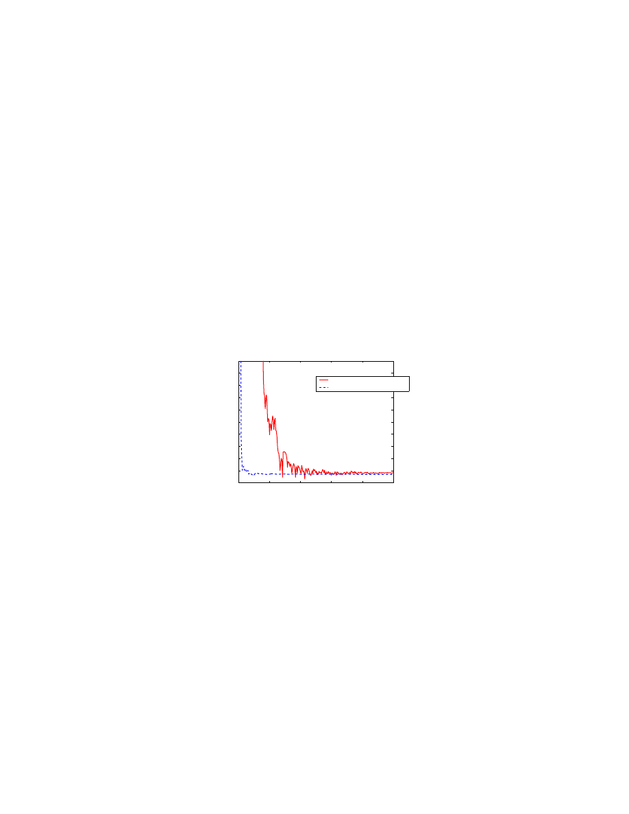
To check the effect of the size of IP address space being monitored, we run the Code Red experiments

again with monitors covering

2

16

IP space. The estimation of infection rate

α as function of time t is

shown in Fig. 11. From it we can see that we can only get relatively accurate estimation of

α after 300

minutes, or when more than 30% of vulnerable computers have been infected. Therefore, the monitoring
system must have enough coverage of IP space in order to get good estimation before it’s too late.

150

200

250

300

350

400

0

0.05

0.1

0.15

0.2

0.25

0.3

0.35

0.4

0.45

0.5

Time t (minute)

α

Observed data
Real number of infected hosts

Fig. 11.

Estimation of Code Red

α ( 2

16

IP space being monitored)

Now we check the effect of initial infected population size. If a future worm uses the “hitlist” technique

to propagate [19], from the monitoring system point of view, the worm has a large number of initially
infected hosts when it begins to propagate. Here we use the same simulation as the previous SQL
experiments except that we increase the initially infected hosts from 10 to 1000. Because the worm’s
high scan traffic at the discrete time 1 will immediately trigger alarm in MWC, we use estimation
algorithms at the beginning.

Fig. 12 compares the worm propagation with different initially infected hosts. The hitlist can dramat-

ically increase the worm spreading speed, but the worm spreading still follows the same dynamics. Fig.
13 shows the estimated value of infection rate

α as time goes on; and Fig. 14 shows the estimated N as

time goes on. For this fast spreading worm, we are still able to estimate both its infection rate and the
vulnerable population at 30 seconds when 10% of vulnerable computers have been infected.

VI. F

UTURE

W

ORKS

Our preliminary study based on simulated Code Red and SQL worms indicate that an early warning

system for Internet worms is feasible. There are, however, some issues need to be studied for an effective

15

0

20

40

60

80

100 120 140 160 180 200

0

1

2

3

4

5

6

7

8

9

10

x 10

4

Time t (second)

Number of infected hosts

10 initially infected hosts
1000 initially infected hosts

Fig. 12.

Worm propagation with

different number of initially infected hosts

0

10

20

30

40

50

60

70

80

0

0.05

0.1

0.15

0.2

0.25

0.3

0.35

0.4

0.45

0.5

Time t (second)

α

Observed data
Real number of infected hosts

Fig. 13.

Estimate infection rate

α

for a worm with hitlist

0

10

20

30

40

50

60

70

80

0

2

4

6

8

10

12

14

x 10

4

Time t (second)

Population N

From estimated

β

From

η

and estimated

α

Fig. 14.

Estimate population

N

for a worm with hitlist

deployment. We briefly discuss them below.

We have assumed a simple epidemic model for our estimation and prediction. While this gives good

results so far, we need to develop more detailed models to reflect the future worm dynamics. For example,
UDP worms could spoof the source addresses to confuse the infection number estimation. Worms could
also vary the scan rates from victim to victim to confuse the scan rate estimation. In the former case
our method can still correctly estimate the scan rate so as to trigger the early warning. In the latter case
worms will be less than maximum possible virulent and there is a need for a game theoretic analysis for
the battle between the worm rate change pattern/virulence and the estimation/mitigation effectiveness.

Our preliminary results apply to the uniform random scan case such as the Code Red and SQL worms.

We need to understand better how the scale of the monitor system should change when worms adopt a
different scanning technique. For example, how large the address space we should monitor for worms
with a local subnet scan? What if worms adapt the strategy of hitlist scan [19]? Especially what if the
attacker install Trojan horses on zombie computers quietly before launching a large scale spreading? Our
system needs to act even faster in these cases, which should be possible since an exponential growth
phase is necessary for a successful attack.

We can select IP address blocks that are owned by but not yet put into use by big ISP’s. From our

analysis result, we see that the number of routable addresses is 10 times higher than the number of hosts
we can find from the DNS table. This means only a small faction of the allocated IP addresses might be
put into use. If we can acquire a list of unused IP address ranges from co-operative ISP’s and monitoring
the traffic toward a random set of them, the attackers might not be able to know which addresses are
under monitoring. We can also apply for many small IP address blocks and use them to do the monitoring
job. Because the address blocks are small, it is hard for the attacker to check all of them to see if they
are used IP addresses. If both the worm and monitoring system dynamically change their strategies, there
could be a game theoretical study.

We need to further study the time step for the discretized filtering algorithm. We may also want to

use a continuous version of the Kalman filter and possible some nonlinear filtering methods, since the
scan observations from a reasonable size of monitoring network would be large enough to be treated as a
continuous time process. The later approach would reduce the significance of the time step size selection
and would work with distributed filtering setting nicely. Actually it is not clear at this point whether a
central processing site would be the best design for the early warning system. Although the total number
of monitors may be on the order of several hundred for the IP V4 address space (with each monitor
covers, for example, 10,000 IP addresses), it could be useful to develop distributed filtering algorithm so

16

as to reduce the latency for the report, which could be important in dealing with fast worms such the
recent SQL worm.

VII. C

ONCLUSIONS

We propose to deploy an early warning system for Internet worms to deliver accurate triggering signal

for mitigation mechanisms. Such system is needed in view of the past worm propagation scale and speed.
Although we have been lucky that the past worms have not been very malicious, the same can not be
said for the future worms. Our analysis and simulation study indicates that such a system is feasible,
and poses many interesting research issues. We hope this paper would generate interest of discussion and
participation in this topic and eventually lead to an effective monitoring and warning system.

VIII. A

CKNOWLEDGEMENT

This work is supported in part by ARO contract DAAD19-01-1-0610; by DARPA under Contract

DOD F30602-00-0554; by NSF under grant EIA-0080119, ANI9980552, ANI-0208116 and by Air Force
Research Lab. Any opinions, findings, and conclusions of the authors do not necessarily reflect the views
of the National Science Foundation.

R

EFERENCES

[1] B.D.O. Anderson and J. Moore. Optimal Filtering. Prentice Hall, 1979.
[2] Cooperative Association for Internet Data Analysis. http://www.caida.org
[3] CERT Advisory. CERT Advisory CA-2002-22 Multiple Vulnerabilities in Microsoft SQL Server. July 29, 2002.

h

ttp://www.cert.org/advisories/CA-2002-22.html

[4] CERT Coordination Center. http://www.cert.org
[5] Z. Chen, L. Gao, and K. Kwiat. Modeling the Spread of Active Worms, IEEE INFOCOM, 2003.
[6] CNN News. Computer worm grounds flights, blocks ATMs.

h

ttp://europe.cnn.com/2003/TECH/internet/01/25/internet.attack/

[7] eEye Digital Security. .ida ”Code Red” Worm. 2001. http://www.eeye.com/html/Research/Advisories/AL20010717.html
[8] eEye Digital Security. CodeRedII Worm Analysis. 2001. http://www.eeye.com/html/Research/Advisories/AL20010804.html
[9] USA Today Technique News. The cost of ’Code Red’: $1.2 billion.

h

ttp://www.usatoday.com/tech/news/2001-08-01-code-red-costs.htm

[10] D.J. Daley and J. Gani. Epidemic Modelling: An Introduction. Cambridge University Press, 1999.
[11] J. C. Frauenthal. Mathematical Modeling in Epidemiology. Springer-Verlag, New York, 1980.
[12] Internet Storm Center. http://isc.incidents.org/
[13] D. Moore. The Spread of Code-Red Worm.

h

ttp://www.caida.org/analysis/security/code-red/coderedv2 analysis.xml

[14] D. Moore, C. Shannon, G. M. Voelker, S. Savage. Internet Quarantine: Requirements for Containing Self-Propagating

Code. Infocom, 2003.

[15] D. Moore, V. Paxson, S. Savage, C. Shannon, S. Staniford, and N. Weaver. The Spread of the Sapphire/Slammer Worm.

h

ttp://www.caida.org/outreach/papers/2003/sapphire/sapphire.html

[16] D. Seeley. A tour of the worm. Proceedings of the Winter Usenix Conference, San Diego, CA, 1989.
[17] Cooperative Association for Internet Data Analysis (CAIDA). Dynamic Graphs of the Nimda worm.

h

ttp://www.caida.org/dynamic/analysis/security/nimda/

[18] SANS Institute. http://www.sans.org
[19] S. Staniford, V. Paxson and N. Weaver. How to Own the Internet in Your Spare Time. 11th Usenix Security Symposium,

San Francisco, August, 2002.

[20] SANS Institute. MS-SQL Server Worm (also called Sapphire, SQL Slammer, SQL Hell).

h

ttp://www.sans.org/alerts/mssql.php

[21] N.C. Weaver. Warhol Worms: The Potential for Very Fast Internet Plagues. 2001.

h

ttp://www.cs.berkeley.edu/ nweaver/warhol.html

[22] G. Welch and G. Bishop. An Introduction to the Kalman Filter. ACM SIGGRAPH, 2001.
[23] C. Zou, W. Gong, and D. Towsley. Code Red Worm Propagation Modeling and Analysis. ACM CCS, 2002.