
KEY CONCEPTS
&
TECHNIQUES
IN
GIS
Albrecht-3572-Prelims.qxd 7/13/2007 4:13 PM Page i

Albrecht-3572-Prelims.qxd 7/13/2007 4:13 PM Page ii

JOCHEN ALBRECHT
KEY CONCEPTS
&
TECHNIQUES
IN
GIS
Albrecht-3572-Prelims.qxd 7/13/2007 4:13 PM Page iii

© Jochen Albrecht 2007
First published 2007
Apart from any fair dealing for the purposes of research or
private study, or criticism or review, as permitted under the
Copyright, Designs and Patents Act, 1988, this publication may
be reproduced, stored or transmitted in any form, or by any
means, only with the prior permission in writing of the publishers,
or in the case of reprographic reproduction, in accordance with the
terms of licences issued by the Copyright Licensing Agency.
Enquiries concerning reproduction outside those terms should be
sent to the publishers.
SAGE Publications Ltd
1 Oliver’s Yard
55 City Road
London EC1Y 1SP
SAGE Publications Inc.
2455 Teller Road
Thousand Oaks, California 91320
SAGE Publications India Pvt Ltd
B1/I I Mohan Cooperative Industrial Area
Mathura Road, New Delhi 110 044
India
SAGE Publications Asia-Pacific Pte Ltd
33 Pekin Street #02-01
Far East Square
Singapore 048763
Library of Congress Control Number 2007922921
British Library Cataloguing in Publication data
A catalogue record for this book is available from
the British Library
ISBN 978-1-4129-1015-6
ISBN 978-1-4129-1016-3 (pbk)
Typeset by C&M Digitals (P) Ltd, Chennai, India
Printed and bound in Great Britain by TJ International Ltd
Printed on paper from sustainable resources
Albrecht-3572-Prelims.qxd 7/13/2007 4:13 PM Page iv

Contents
List of Figures
ix
Preface xi
1
Creating Digital Data
1
1.1
Spatial data
2
1.2
Sampling
3
1.3
Remote sensing
5
1.4
Global positioning systems
7
1.5
Digitizing and scanning
8
1.6
The attribute component of geographic data
8
2
Accessing Existing Data
11
2.1
Data exchange
11
2.2
Conversion
12
2.3
Metadata
13
2.4
Matching geometries (projection and coordinate systems)
13
2.5
Geographic web services
15
3
Handling Uncertainty
17
3.1
Spatial data quality
17
3.2
How to handle data quality issues
19
4
Spatial Search
21
4.1
Simple spatial querying
21
4.2
Conditional querying
22
4.3
The query process
23
4.4
Selection
24
4.5
Background material: Boolean logic
25
5
Spatial Relationships
29
5.1
Recoding
29
5.2
Relationships between measurements
32
5.3
Relationships between features
34
Albrecht-3572-Prelims.qxd 7/13/2007 4:13 PM Page v

6
Combining Spatial Data
37
6.1
Overlay
37
6.2
Spatial Boolean logic
40
6.3
Buffers
41
6.4
Buffering in spatial search
43
6.5
Combining operations
43
6.6
Thiessen polygons
44
7
Location-Allocation
45
7.1
The best way
45
7.2
Gravity model
46
7.3
Location modeling
47
7.4
Allocation modeling
50
8
Map Algebra
51
8.1
Raster GIS
51
8.2
Local functions
53
8.3
Focal functions
55
8.4
Zonal functions
56
8.5
Global functions
57
8.6
Map algebra scripts
58
9
Terrain Modeling
59
9.1
Triangulated irregular networks (TINs)
60
9.2
Visibility analysis
61
9.3
Digital elevation and terrain models
62
9.4
Hydrological modeling
63
10
Spatial Statistics
65
10.1 Geo-statistics
65
10.1.1
Inverse distance weighting
65
10.1.2
Global and local polynomials
66
10.1.3
Splines
67
10.1.4
Kriging
69
10.2 Spatial analysis
70
10.2.1
Geometric descriptors
70
10.2.2
Spatial patterns
72
10.2.3
The modifiable area unit problem (MAUP)
74
10.2.4
Geographic relationships
75
vi
CONTENTS
Albrecht-3572-Prelims.qxd 7/13/2007 4:13 PM Page vi

11
Geocomputation
77
11.1 Fuzzy reasoning
77
11.2 Neural networks
79
11.3 Genetic algorithms
80
11.4 Cellular automata
81
11.5 Agent-based modeling systems
82
12
Epilogue: Four-Dimensional Modeling
85
Glossary
89
References
95
Index
99
CONTENTS
vii
Albrecht-3572-Prelims.qxd 7/13/2007 4:13 PM Page vii

Albrecht-3572-Prelims.qxd 7/13/2007 4:13 PM Page viii

List of Figures
Figure 1
Object vs. field view (vector vs. raster GIS)
3
Figure 2
Couclelis’ ‘Hierarchical Man’
4
Figure 3
Illustration of variable source problem
5
Figure 4
Geographic relationships change according to scale
6
Figure 5
One geography but many different maps
12
Figure 6
Subset of a typical metadata tree
14
Figure 7
The effect of different projections
15
Figure 8
Simple query by location
22
Figure 9
Conditional query or query by (multiple) attributes
23
Figure 10
The relationship between spatial and attribute query
24
Figure 11
Partial and complete selection of features
25
Figure 12
Using one set of features to select another set
26
Figure 13
Simple Boolean logic operations
26
Figure 14
Typical soil map
30
Figure 15
Recoding as simplification
30
Figure 16
Recoding as a filter operation
31
Figure 17
Recoding to derive new information
31
Figure 18
Four possible spatial relationships in a pixel world
33
Figure 19
Simple (top row) and complex (bottom row) geometries
33
Figure 20
Pointer structure between tables of feature geometries
34
Figure 21
Part of the New York subway system
35
Figure 22
Topological relationships between features
35
Figure 23
Schematics of a polygon overlay operation
38
Figure 24
Overlay as a coincidence function
38
Figure 25
Overlay with multiple input layers
39
Figure 26
Spatial Boolean logic
40
Figure 27
The buffer operation in principle
41
Figure 28
Inward or inverse buffer
42
Figure 29
Corridor function
42
Figure 30
Surprise effects of buffering affecting towns
outside a flood zone
43
Figure 31
Thiessen polygons
44
Albrecht-3572-Prelims.qxd 7/13/2007 4:13 PM Page ix

Figure 32
Areas of influence determining the reach
of gravitational pull
47
Figure 33
Von Thünen’s agricultural zones around a market
48
Figure 34
Weber’s triangle
48
Figure 35
Christaller’s Central Place theory
49
Figure 36
Origin-destination matrix
50
Figure 37
The spatial scope of raster operations
52
Figure 38
Raster organization and cell position addressing
52
Figure 39
Zones of raster cells
53
Figure 40
Local function
54
Figure 41
Multiplication of a raster layer by a scalar
54
Figure 42
Multiplying one layer by another one
55
Figure 43
Focal function
55
Figure 44
Averaging neighborhood function
56
Figure 45
Zonal function
57
Figure 46
Value grids as spatial lookup tables
58
Figure 47
Three ways to represent the third dimension
59
Figure 48
Construction of a TIN
60
Figure 49
Viewshed
61
Figure 50
Derivation of slope and aspect
62
Figure 51
Flow accumulation map
63
Figure 52
Inverse distance weighting
66
Figure 53
Polynomials of first and second order
67
Figure 54
Local and global polynomials
67
Figure 55
Historical use of splines
68
Figure 56
Application of splines to surfaces
68
Figure 57
Exact and inexact interpolators
69
Figure 58
Geometric mean
71
Figure 59
Geometric mean and geometric median
72
Figure 60
Standard deviational ellipse
73
Figure 61
Shape measures
73
Figure 62
Joint count statistic
74
Figure 63
Shower tab illustrating fuzzy notions
of water temperature
78
Figure 64
Schematics of a single neuron
79
Figure 65
Genetic algorithms
81
Figure 66
Principles of genetic algorithms
82
x
LIST OF FIGURES
Albrecht-3572-Prelims.qxd 7/13/2007 4:13 PM Page x

Preface
GIS has been coming of age. Millions of people use one GIS or another every day,
and with the advent of Web 2.0 we are promised GIS functionality on virtually every
desktop and web-enabled cellphone. GIS knowledge, once restricted to a few insid-
ers working with minicomputers that, as a category, don’t exist any more, has
proliferated and is bestowed on students at just about every university and increasingly
in community colleges and secondary schools. GIS textbooks abound and in the
course of 20 years have moved from specialized topics (Burrough 1986) to
general-purpose textbooks (Maantay and Ziegler 2006). With such a well-informed
user audience, who needs yet another book on GIS?
The answer is two-fold. First, while there are probably millions who use GIS,
there are far fewer who have had a systematic introduction to the topic. Many are
self-trained and good at the very small aspect of GIS they are doing on an everyday
basis, but they lack the bigger picture. Others have learned GIS somewhat system-
atically in school but were trained with a particular piece of software in mind – and
in any case were not made aware of modern methods and techniques. This book also
addresses decision-makers of all kinds – those who need to decide whether they
should invest in GIS or wait for GIS functionality in Google Earth (Virtual Earth if
you belong to the other camp).
This book is indebted to two role models. In the 1980s, Sage published a tremend-
ously useful series of little green paperbacks that reviewed quantitative methods,
mostly for the social sciences. They were concise, cheap (as in extremely good quality/
price ratio), and served students and practitioners alike. If this little volume that you
are now holding contributes to the revival of this series, then I consider my task to
be fulfilled. The other role model is an unsung hero, mostly because it served such
a small readership. The CATMOG (Concepts and Techniques in Modern
Geography) series fulfills the same set of criteria and I guess it is no coincidence that
it too has been published by Sage. CATMOG is now unfortunately out of print but
deserves to be promoted to the modern GIS audience at large, which as I pointed out
earlier, is just about everybody. With these two exemplars of the publishing pan-
theon in house, is it a wonder that I felt honored to be invited to write this volume?
My kudos goes to the unknown editors of these two series.
Jochen Albrecht
Albrecht-3572-Prelims.qxd 7/13/2007 4:13 PM Page xi

Albrecht-3572-Prelims.qxd 7/13/2007 4:13 PM Page xii

The creation of spatial data is a surprisingly underdeveloped topic in GIS literature.
Part of the problem is that it is a lot easier to talk about tangibles such as data as a
commodity, and digitizing procedures, than to generalize what ought to be the very
first step: an analysis of what is needed to solve a particular geographic question.
Social sciences have developed an impressive array of methods under the umbrella
of research design, originally following the lead of experimental design in the natu-
ral sciences but now an independent body of work that gains considerably more
attention than its counterpart in the natural sciences (Mitchell and Jolley 2001).
For GIScience, however, there is a dearth of literature on the proper development
of (applied) research questions; and even outside academia there is no vendor-
independent guidance for the GIS entrepreneur on setting up the databases that off-
the-shelf software should be applied to. GIS vendors try their best to provide their
customers with a starter package of basic data; but while this suffices for training or
tutorial purposes, it cannot substitute for in-house data that is tailored to the needs
of a particular application area.
On the academic side, some of the more thorough introductions to GIS (e.g.
Chrisman 2002) discuss the history of spatial thought and how it can be expressed
as a dialectic relationship between absolute and relative notions of space and time,
which in turn are mirrored in the two most common spatial representations of raster
and vector GIS. This is a good start in that it forces the developer of a new GIS data-
base to think through the limitations of the different ways of storing (and acquiring)
spatial data, but it still provides little guidance.
One of the reasons for the lack of literature – and I dare say academic research –
is that far fewer GIS would be sold if every potential buyer knew how much work
is involved in actually getting started with one’s own data. Looking from the ivory
tower, there are ever fewer theses written that involve the collection of relevant data
because most good advisors warn their mentees about the time involved in that task
and there is virtually no funding of basic research for the development of new meth-
ods that make use of new technologies (with the exception of remote sensing where
this kind of research is usually funded by the manufacturer). The GIS trade maga-
zines of the 1980s and early 90s were full of eye-witness reports of GIS projects
running over budget; and a common claim back then was that the development of
the database, which allows a company or regional authority to reap the benefits
of the investment, makes up approximately 90% of the project costs. Anecdotal
evidence shows no change in this staggering character of GIS data assembly
(Hamil 2001).
1
Creating Digital Data
Albrecht-3572-Ch-01.qxd 7/13/2007 4:14 PM Page 1

So what are the questions that a prospective GIS manager should look into before
embarking on a GIS implementation? There is no definitive list, but the following
questions will guide us through the remainder of this chapter.
•
What is the nature of the data that we want to work with?
•
Is it quantitative or qualitative?
•
Does it exist hidden in already compiled company data?
•
Does anybody else have the data we need? If yes, how can we get hold of it? See
also Chapter 2.
•
What is the scale of the phenomenon that we try to capture with our data?
•
What is the size of our study area?
•
What is the resolution of our sampling?
•
Do we need to update our data? If yes, how often?
•
How much data do we need, i.e. a sample or a complete census?
•
What does it cost? An honest cost–benefit analysis can be a real eye-opener.
Although by far the most studied, the first question is also the most difficult one
(Gregory 2003). It touches upon issues of research design and starts with a set of
goals and objectives for setting up the GIS database. What are the questions that we
would like to get answered with our GIS? How immutable are those questions – in
other words, how flexible does the setup have to be? It is a lot easier (and hence
cheaper) to develop a database to answer one specific question than to develop a
general-purpose system. On the other hand, it usually is very costly and sometimes
even impossible to change an existing system to answer a new set of questions.
The next step is then to determine what, in an ideal world, the data would look
like that answers our question(s). Our world is not ideal and it is unlikely that we
will gather the kind of data prescribed in this step, but it is interesting to understand
the difference between what we would like to have and what we actually get.
Chapter 3 will expand on the issues related to imperfect data.
1.1 Spatial data
In its most general form, geographic data can be described as any kind of data that
has a spatial reference. A spatial reference is a descriptor for some kind of location,
either in direct form expressed as a coordinate or an address or in indirect form rel-
ative to some other location. The location can (1) stand for itself or (2) be part of a
spatial object, in which case it is part of the boundary definition of that object.
In the first instance, we speak of a field view of geographic information because
all the attributes associated with that location are taken to accurately describe
everything at that very position but are to be taken less seriously the further we get
away from that location (and the closer we can to another location).
The second type of locational reference is used for the description of geographic
objects. The position is part of a geometry that defines the boundary of that object.
2
KEY CONCEPTS AND TECHNIQUES IN GIS
Albrecht-3572-Ch-01.qxd 7/13/2007 4:14 PM Page 2
The attributes associated with this piece of geographic data are supposed to be valid
for all coordinates that are part of the geographic object. For example, if we have the
attribute ‘population density’ for a census unit, then the density value is assumed to
be valid throughout this unit. This would obviously be unrealistic in the case where
a quarter of this unit is occupied by a lake, but it would take either lots of auxiliary
information or sophisticated techniques to deal with this representational flaw.
Temporal aspects are treated just as another attribute. GIS have only very limited
abilities to reason about temporal relationships.
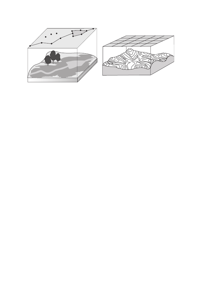
This very general description of spatial data is slightly idealistic (Couclelis 1992). In
practice, most GIS distinguish strictly between the two types of spatial perspectives – the
field view that is typically represented using raster GIS, versus the object view
exemplified by vector GIS (see Figure 1). The sets of functionalities differ consid-
erably depending on which perspective is adopted.
1.2 Sampling
But before we get there, we will have to look at the relationship between the real-
world question and the technological means that we have to answer it. Helen
Couclelis (1982) described this process of abstracting from the world that we live in
to the world of GIS in the form of a ‘hierarchical man’ (see Figure 2). GIS store their
spatial data in a two-dimensional Euclidean geometry representation, and while even
spatial novices tend to formalize geographic concepts as simple geometry, we all
realize that this is not an adequate representation of the real world. The hierarchical
man illustrates the difference between how we perceive and conceptualize the world
and how we represent it on our computers. This in turn then determines the kinds of
questions (procedures) that we can ask of our data.
This explains why it is so important to know what one wants the GIS to answer.
It starts with the seemingly trivial question of what area we should collect the data
for – ‘seemingly’ because, often enough, what we observe for one area is influenced
by factors that originate from outside our area of interest. And unless we have
CREATING DIGITAL DATA
3
32.3
x,y
x,y
x,y
x,y
x,y
x,y
x,y
x,y
x,y
x,y
x,y
x,y
x,y
x,y
x,y
40.8
41.8
43.0
36.1
36.2
32.6
31.1
30.4
31.2
30.6
32.7
33.5
33.6
35.1
33.0
34.6
33.1
31.2
34.9
Figure 1
Object vs. field view (vector vs. raster GIS)
Albrecht-3572-Ch-01.qxd 7/13/2007 4:14 PM Page 3

complete control over all aspects of all our data, we might have to deal with bound-
aries that are imposed on us but have nothing to do with our research question (the
modifiable area unit problem, or MAUP, which we will revisit in Chapter 10). An
example is street crime, where our outer research boundary is unlikely to be related
to the city boundary, which might have been the original research question, and
where the reported cases are distributed according to police precincts, which in turn
would result in different spatial statistics if we collected our data by precinct rather
than by address (see Figure 3).
In 99% of all situations, we cannot conduct a complete census – we cannot inter-
view every customer, test every fox for rabies, or monitor every brown field (former
industrial site). We then have to conduct a sample and the techniques involved are
radically different depending on whether we assume a discrete or continuous distri-
bution and what we believe the causal factors to be. We deal with a chicken-and-egg
dilemma here because the better our understanding of the research question, the
more specific and hence appropriate can be our sampling technique. Our needs,
however, are exactly the other way around. With a generalist (‘if we don’t know any-
thing, let’s assume random distribution’) approach, we are likely to miss the crucial
events that would tell us more about the unknown phenomenon (be it West Nile virus
or terrorist chatter).
4
KEY CONCEPTS AND TECHNIQUES IN GIS
H
1
Real Space
H
2
Conditioned Space
Use Space
H
3
Rated Space
H
4
Adapted Space
H
5
Standard Space
H
K-1
Euclidean Space
H
K
Figure 2
Couclelis’ ‘Hierarchical Man’
Albrecht-3572-Ch-01.qxd 7/13/2007 4:14 PM Page 4

Most sampling techniques apply to so-called point data; i.e., individual locations
are sampled and assumed to be representative for their immediate neighborhood.
Values for non-sampled locations are then interpolated assuming continuous distri-
butions. The interpolation techniques will be discussed in Chapter 10. Currently
unresolved are the sampling of discrete phenomena, and how to deal with spatial
distributions along networks, be they river or street networks.
Surprisingly little attention has been paid to the appropriate scale for sampling.
A neighborhood park may be the world to a squirrel but is only one of many possi-
ble hunting grounds for the falcon nesting on a nearby steeple (see Figure 4). Every
geographic phenomenon can be studied at a multitude of scales but usually only a
small fraction of these is pertinent to the question at hand. As mentioned earlier,
knowing what one is after goes a long way in choosing the right approach.
Given the size of the study area, the assumed form of spatial distribution and
scale, and the budget available, one eventually arrives at a suitable spatial resolution.
However, this might be complicated by the fact that some spatial distributions
change over time (e.g. people on the beach during various seasons). In the end, one
has to make sure that one’s sampling represents, or at least has a chance to represent,
the phenomenon that the GIS is supposed to serve.
1.3 Remote sensing
Without wasting too much time on the question whether remotely sensed data is pri-
mary or secondary data, a brief synopsis of the use of image analysis techniques as
a source for spatial data repositories is in order. Traditionally, the two fields of GIS
and remote sensing were cousins who acknowledged each other’s existence but
otherwise stayed clearly away from each other. The widespread availability of remotely
sensed data and especially pressure from a range of application domains have forced
the two communities to cross-fertilize. This can be seen in the added functionalities
of both GIS and remote sensing packages, although the burden is still on the user to
extract information from remotely sensed data.
CREATING DIGITAL DATA
5
Census
Voting District
Police
Armed Robbery
Assaults
Figure 3
Illustration of variable source problem
Albrecht-3572-Ch-01.qxd 7/13/2007 4:14 PM Page 5

Originally, GIS and remote sensing data were truly complimentary by adding con-
text to the respective other. GIS data helped image analysts to classify otherwise
ambiguous pixels, while imagery used as backdrop to highly specialized vector data
provides orientation and situational setting. Truly integrated software that mixes and
matches raster, vector and image data for all kinds of GIS functions does not exist;
at best, some raster analytical functions take vector data as determinants of process-
ing boundaries. To make full use of remotely sensed data, the GIS user needs to
understand the characteristics of a wide range of sensors and what kind of manipu-
lation the imagery has undergone before it arrives on the user’s desk.
Remotely sensed data is a good example for the field view of spatial information
discussed earlier. For each location we are given a value, called digital number
(DN), usually in the range from 0 to 255, sometimes up to 65,345. These digital
numbers are visualized by different colors on the screen but the software works with
DN values rather than with colors. The satellite or airborne sensors have different
6
KEY CONCEPTS AND TECHNIQUES IN GIS
Figure 4
Geographic relationships change according to scale
Albrecht-3572-Ch-01.qxd 7/13/2007 4:14 PM Page 6

sensitivities in a wide range of the electromagnetic spectrum, and one aspect that is
confusing for many GIS users is that the relationship between a color on the screen and
a DN representing a particular but very small range of the electromagnetic spectrum is
arbitrary. This is unproblematic as long as we leave the analysis entirely to the
computer – but there is only a very limited range of tasks that can be performed auto-
matically. In all other instances we need to understand what a screen color stands for.
Most remotely sensed data comes from so-called passive sensors, where the sen-
sor captures reflections of energy of the earth’s surface that originally comes from
the sun. Active sensors on the other hand send their own signal and allow the image
analyst to make sense of the difference between what was sent off and what bounces
back from the ‘surface’. In either instance, the word surface refers either to the topo-
graphic surface or to parts in close vicinity, such as leaves, roofs, minerals or water
in the ground. Early generations of sensors captured reflections predominantly in a
small number of bands of the visible (to the human eye) and infrared ranges, but the
number of spectral bands as well as their distance from the visible range has
increased. In addition, the resolution of images has improved from multiple kilo-
meters to fractions of a meter (or centimeters in the case of airborne sensors).
With the right sensor, software and expertise of the operator we can now use
remotely sensed data to distinguish not only various kinds of crops but also their
maturity, response to drought conditions or mineral deficiencies. We can detect
buried archaeological sites, do mineral exploration, and measure the height of
waves. But all of these require a thorough understanding of what each sensor can
and cannot capture as well as what conceptual model image analysts use to draw
their conclusions from the digital numbers mentioned above. The difference
between academic theory and operational practice is often discouraging. This author,
for instance, searched in vain for imagery that helps to discern the vanishing rate of
Irish bogs because for many years there happened to be no coincidence between
cloudless days and a satellite over these areas on a clear day.
On the upside, once one has the kind of remotely sensed data that the GIS practi-
tioner is looking for and some expertise in manipulating it (see Chapter 8), then the
options for improved GIS applications are greatly enhanced.
1.4 Global positioning systems
Usually, when we talk about remotely sensed data, we are referring to imagery – that
is, a file that contains reflectance values for many points covering a given rectangular
area. The global positioning system (GPS) is also based on satellite data, but the data
consists of positions only – there is no attribute information other than some metadata
on how the position was determined. Another difference is that GPS data can be col-
lected on a continuing basis, which helps to collect not just single positions but also
route data. In other words, while a remotely sensed image contains data about a lot of
neighboring locations that gets updated on a daily to yearly basis, GPS data potentially
consist of many irregularly spaced points that are separated by seconds or minutes.
CREATING DIGITAL DATA
7
Albrecht-3572-Ch-01.qxd 7/13/2007 4:14 PM Page 7

As of 2006, there was only one easily accessible GPS world-wide. The Russian
system as well as alternative military systems are out of reach of the typical GIS
user, and the planned civilian European system will not be functional for a number
of years. Depending on the type of receiver, ground conditions, and satellite con-
stellations, the horizontal accuracy of GPS measurements lies between a few cen-
timeters and a few hundred meters, which is sufficient for most GIS applications
(however, buyer beware: it is never as good as vendors claim).
GPS data is mainly used to attach a position to field data – that is, to spatialize
attribute measurements taken in the field. It is preferable for the two types of meas-
urement to be taken concurrently because this decreases the opportunity for errors in
matching measurements with their corresponding position. GPS data is increasingly
augmented by a new version of triangulating one’s position that is based on cell-
phone signals (Bryant 2005). Here, the three or more satellites are either replaced or
preferably added to by cellphone towers. This increases the likelihood of having a
continuous signal, especially in urban areas, where buildings might otherwise dis-
rupt GPS reception. Real-time applications especially benefit from the ability to
track moving objects this way.
1.5 Digitizing and scanning
Most spatial legacy data exists in the form of paper maps, sketches or aerial photo-
graphs. And although most newly acquired data comes in digital format, legacy data
holds potentially enormous amounts of valuable information. The term digitizing is
usually applied to the use of a special instrument that allows interactive tracing of
the outline of features on an analogue medium (mostly paper maps). This is in con-
trast to scanning, where an instrument much like a photocopying or fax machine
captures a digital image of the map, picture or sketch. The former creates geometries
for geographic objects, while the latter results in a picture much like early uses of
imagery to provide a backdrop for pertinent geometries.
Nowadays, the two techniques have merged in what is sometimes called on-
screen or heads-up digitizing, where a scanned image is loaded into the GIS and the
operator then traces the outline of objects of their choice on the screen. In any case,
and parallel to the use of GPS measurements, the result is a file of mere geometries,
which then have to be linked with the attribute data describing each geographic
object. Outsiders keep being surprised how little the automatic recognition of objects
has been advanced and hence how much labor is still involved in digitizing or scan-
ning legacy data.
1.6 The attribute component of geographic data
Most of the discussion above concerns the geometric component of geographic
information. This is because it is the geometric aspects that make spatial data
8
KEY CONCEPTS AND TECHNIQUES IN GIS
Albrecht-3572-Ch-01.qxd 7/13/2007 4:14 PM Page 8

special. Handling of the attributes is pretty much the same as for general-purpose
data handling, say in a bank or a personnel department. Choice of the correct
attribute, questions of classification, and error handling are all important topics; but,
in most instances, a standard textbook on database management would provide an
adequate introduction.
More interesting are concerns arising from the combination of attributes and
geometries. In addition to the classical mismatch, we have to pay special attention
to a particular geographic form of ecological fallacy. Spatial distributions are hardly
ever uniform within a unit of interest, nor are they independent of scale.
CREATING DIGITAL DATA
9
Albrecht-3572-Ch-01.qxd 7/13/2007 4:14 PM Page 9

Albrecht-3572-Ch-01.qxd 7/13/2007 4:14 PM Page 10

Most GIS users will start using their systems by accessing data compiled either by
the GIS vendor or by the organization for which they work. Introductory tutorials
tend to gloss over the amount of work involved even if the data does not have to be
created from scratch. Working with existing data starts with finding what’s out there
and what can be rearranged easily to fulfill one’s data requirements. We are currently
experiencing a sea change that comes under the buzz word of interoperability.
GISystems and the data that they consist of used to be insular enterprises, where
even if two parties were using the same software, the data had to exported to an
exchange format. Nowadays different operating systems do not pose any serious
challenge to data exchange any more, and with ubiquitous WWW access, the
remaining issues are not so much technical in nature.
2.1 Data exchange
Following the logic of geographic data structure outlined in Chapter 1, data
exchange has to deal with two dichotomies, the common (though not necessary) dis-
tinction between geometries and attributes, and the difference between the geo-
graphic data on the one hand and its cartographic representation on the other.
Let us have a closer look at the latter issue. Geographic data is stored as a combina-
tion of locational, attribute and possibly temporal components, where the locational part
is represented by a reference to a virtual position or a boundary object. This locational
part can be represented in many different ways – usually referred to as the mapping of
a given geography. This mapping is often the result of a very laborious process of com-
bining different types of geographic data, and if successful, tells us a lot more than the
original tables that it is made up of (see Figure 5). Data exchange can then be seen
as (1) the exchange of the original geography, (2) the exchange of only the map
graphics – that is, the map symbols and their arrangement, or (3) the exchange of both.
The translation from geography to map is a proprietary process, in addition to the user’s
decisions of how to represent a particular geographic phenomenon.
The first thirty years of GIS saw the exchange mainly of ASCII files in a propri-
etary but public format. These exchange files are the result of an export operation
and have to be imported rather than directly read into the second system. Recent
standardization efforts led to a slightly more sophisticated exchange format based on
the Web’s extensible markup language, XML. The ISO standards, however, cover
only a minimum of commonality across the systems and many vendor-specific
features are lost during the data exchange process.
2
Accessing Existing Data
Albrecht-3572-Ch-02.qxd 7/13/2007 5:07 PM Page 11

12
KEY CONCEPTS AND TECHNIQUES IN GIS
2.2 Conversion
Data conversion is the more common way of incorporating data into one’s GIS project.
It comprises three different aspects that make it less straightforward than one might
assume. Although there are literally hundreds of GIS vendors, each with their own
proprietary way of storing spatial information, they all have ways of storing data
using one of the de-facto standards for simple attributes and geometry. These used
to be dBASE™ and AutoCAD™ exchange files but have now been replaced by the
published formats of the main vendors for combined vector and attribute data, most
prominently the ESRI shape file format, and the GeoTIFF™ format for pixel-based
data. As there are hundreds of GIS products, the translation between two less com-
mon formats can be fraught with high information loss and this translation process
has become a market of its own (see, for example, SAFE Corp’s feature manipula-
tion engine FME).
The second conversion aspect is more difficult to deal with. Each vendor, and
arguably even more GIS users, have different ideas of what constitutes a geographic
object. The translation of not just mere geometry but the semantics of what is
encoded in a particular vendor’s scheme is a hot research topic and has sparked a
whole new branch of GIScience dealing with the ontologies of representing geography.
A glimpse of the difficulties associated with translating between ontologies can be
gathered from the differences between a raster and a vector representation of a geo-
graphic phenomenon. The academic discussion has gone beyond the raster/vector
Figure 5
One geography but many different maps
Albrecht-3572-Ch-02.qxd 7/13/2007 5:07 PM Page 12

ACCESSING EXISTING DATA
13
debate, but at the practical level this is still the cause of major headaches, which can
be avoided only if all potential users of a GIS dataset are involved in the original
definition of the database semantics. For example, the description of a specific
shoal/sandbank depends on whether one looks at it as an obstacle (as depicted on a
nautical chart) or as a seal habitat, which requires parts to be above water at all times
but defines a wider buffer of no disturbance than is necessary for purely naviga-
tional purposes.
The third aspect has already been touched upon in the section on data exchange –
the translation from geography to map data. In addition to the semantics of
geographic features, a lot of effort goes into the organization of spatial data. How
complex can individual objects be? Can different vector types be mixed, or vector
and raster definitions of a feature? What about representations at multiple scales? Is
the projection part of the geographic data or the map (see next section)? There are
many ways to skin a cat. And these ways are virtually impossible to mirror in a con-
version from one system to another. One solution is to give up on the exchange of
the underlying geographic data and to use a desktop publishing or web-based SVG
format to convert data from and to. These provide users with the opportunity to alter
the graphical representation. The ubiquitous PDF format, on the other hand, is con-
venient because it allows the exchange of maps regardless of the recipient’s output
device but it is a dead end because it cannot be converted into meaningful map or
geography data.
2.3 Metadata
All of the above options for conversion depend on a thorough documentation of the
data to be exchanged or converted. This area has seen the greatest progress in recent
years as ISO standard 19115 has been widely adopted across the world and across
many disciplines (see Figure 6). A complete metadata specification of a geospatial
dataset is extremely labor-intensive to compile and can be expected only for relatively
new datasets, but many large private and government organizations mandate a proper
documentation, which will eventually benefit the whole geospatial community.
2.4 Matching geometries (projection and coordinate systems)
There are two main reasons why geographic data cannot be adequately represented
by simple geometries used in popular computer aided design (CAD) programs. The
first is that projects covering more than a few square kilometers have to deal with
the curvature of the Earth. If we want to depict something that is little under the
horizon, then we need to come up with ways to flatten the earth to fit into our
two-dimensional computer world. The other reason is that, even for smaller areas,
where the curvature could be neglected, the need to combine data from different
sources, especially satellite imagery – requires matching coordinates from different
Albrecht-3572-Ch-02.qxd 7/13/2007 5:07 PM Page 13

14
KEY CONCEPTS AND TECHNIQUES IN GIS
coordinate systems. The good news is that most GIS these days relieve us from the
burden of translating between the hundreds of projections and coordinate systems.
The bad news is that we still need to understand how this works to ask the right ques-
tions in case the metadata fails to report on these necessities.
Contrary to Dutch or Kansas experiences as well as the way we store data in a
GIS, the Earth is not flat. Given that calculations in spherical geometry are very
complicated, leading to rounding errors, and that we have thousands of calculations
performed each time we ask the GIS to do something, manufacturers have decided
to adopt the simple two-dimensional view of a paper map. Generations of cartogra-
phers have developed a myriad of ways to map positions on a sphere to coordinates
on flat paper. Even the better of these projections all have some flaws and the main
difference between projections is the kind of distortion that they introduce to the data
(see Figure 7). It is, for example, impossible to design a map that measures the
distances between all cities correctly. We can have a table that lists all these dis-
tances but there is no way to draw them properly on a two-dimensional surface.
Many novices to geographic data confuse the concepts of projections and coordinate
systems. The former just describes the way we project points from a sphere on to a flat
surface. The latter determines how we index positions and perform measurements on the
result of the projection process. The confusion arises from the fact that many geographic
Figure 6
Subset of a typical metadata tree
Metadata
Identification Information
Citation
Description
Time Period of Content
Status
Spatial Reference
Horizontal Coordinate System Definition: planar
Map Projection: Lambert conformal conic
Standard parallel: 43.000000
Standard parallel: 45.500000
Longitude of Central Meridian: –120.500000
Latitude of Projection Origin: 41.750000
False Easting: 1312336.000000
False Northing: 0.000000
Abcissa Resolution: 0.004096
Ordinate Resolution: 0.004096
Horizontal Datum: NAD83
Ellipsoid: GRS80
Semi-major Axis: 6378137.000000
Flattening Ratio: 298.572222
Keywords
Access Constraints
Reference Information
Metadata Date
Metadata Contact
Metadata Standard Name
Metadata Standard Version
Albrecht-3572-Ch-02.qxd 7/13/2007 5:07 PM Page 14

ACCESSING EXISTING DATA
15
coordinate systems consist of projections and a mathematical coordinate system, and that
sometimes the same name is used for a geographic coordinate system and the projec-
tion(s) it is based on (e.g. the Universal Transverse Mercator or UTM system). In addi-
tion, geographic coordinate systems differ in their metric (do the numbers that make up
a coordinate represent feet, meters or decimal degrees?), the definition of their origin,
and the assumed shape of the Earth, also known as its geodetic datum. It goes beyond
the scope of this book to explain all these concepts but the reader is invited to visit the
USGS website at http://erg.usgs.gov/isb/pubs/factsheets/fs07701.html for more informa-
tion on this subject.
Sometimes (e.g. when we try to incorporate old sketches or undocumented maps),
we do not have the information that a GIS needs to match different datasets. In that
case, we have to resort to a process known as rubber sheeting, where we interac-
tively try to link as many individually identifiable points in both datasets to gain
enough information to perform a geometric transformation. This assumes that we
have one master dataset whose coordinates we trust and an unknown or untrusted
dataset whose coordinates we try to improve.
2.5 Geographic web services
The previous sections describe a state of data acquisition, which is rapidly becom-
ing outdated in some application areas. Among the first questions that one should
ask oneself before embarking on a GIS project is how unique is this project? If it is
not too specialized then chances are that there is a market for providing this service
or at least the data for it. This is particularly pertinent in application areas where the
geography changes constantly, such as a weather service, traffic monitoring, or real
estate markets. Here it would be prohibitively expensive to constantly collect data
Figure 7
The effect of different projections
Lambert Conformal Conic
Winkel Tripel
Mollweide
Orthographic
Azimuthal Equidistant
Albrecht-3572-Ch-02.qxd 7/13/2007 5:07 PM Page 15

for just one application and one should look for either data or if one is lucky even
the analysis results on the web.
Web-based geographic data provision has come a long (and sometimes unex-
pected) way. In the 1990s and the first few years of the new millennium, the empha-
sis was on FTP servers and web portals that provided access to either public domain
data (the USGS and US Census Bureau played a prominent role in the US) or to
commercial data, most commonly imagery. Standardization efforts, especially those
aimed at congruence with other IT standards, helped geographic services to become
mainstream. Routing services (like it or not, MapQuest has become a household
name for what geography is about), neighborhood searches such as local.yahoo.com,
and geodemographics have helped to catapult geographic web services out of the
academic realm and into the marketplace. There is an emerging market for non-GIS
applications that are yet based on the provision of decentralized geodata in the
widest sense. Many near real-time applications such as sending half a million
volunteers on door-to-door canvassing during the 2004 presidential elections in the
US, the forecast of avalanche risks and subsequent day-to-day operation of ski lifts
in the European Alps, or the coordination of emergency management efforts during
the 2004 tsunami have only been possible because of the interoperability of web
services.
The majority of web services are commercial, accessible only for a fee (commer-
cial providers might have special provisions in case of emergencies). As this is a
very new market, the rates are fluctuating and negotiable but can be substantial if
there are many (as in millions) individual queries. The biggest potential lies in the
emergence of middle-tier applications not aimed at the end user that are based on
raw data and transform these to be combined with other web services. Examples
include concierge services that map attractions around hotels with continuously
updated restaurant menus, department store sales, cinema schedules, etc., or a nature
conservation website that continuously maps GPS locations of collared elephants in
relationship to updated satellite imagery rendered in a 3-D landscape that changes
according to the direction of the track. In some respect, this spells the demise of GIS
as we know it because the tasks that one would usually perform in a GIS are now
executed on a central server that combines individual services the same way that an
end consumer used to combine GIS functions. Similar to the way that a Unix shell
script programmer combines little programs to develop highly customized applica-
tions, web services application programmers now combine traditional GIS function-
ality with commercial services (like the one that performs a secure credit card
transaction) to provide highly specialized functionality at a fraction of the price of a
GIS installation.
This form of outsourcing can have great economical benefits and, as in the case
of emergency applications, may be the only way to compile crucial information at
short notice. But it comes at the price of losing control over how data is combined.
The next chapter will deal with this issue of quality control in some detail.
16
KEY CONCEPTS AND TECHNIQUES IN GIS
Albrecht-3572-Ch-02.qxd 7/13/2007 5:07 PM Page 16

The only way to justifiably be confident about the data one is working with is to
collect all the primary data oneself and to have complete control over all aspects of
acquisition and processing. In the light of the costs involved in creating or accessing
existing data this is not a realistic proposition for most readers.
GIS own their right of existence to their use in a larger spatial decision-making
process. By basing our decisions on GIS data and procedures, we put faith in the
truthfulness of the data and the appropriateness of the procedures. Practical experi-
ence has tested that faith often enough for the GIS community to come up with ways
and means to handle the uncertainty associated with data and procedures over which
we do not have complete control. This chapter will introduce aspects of spatial data
quality and then discuss metadata management as the best method to deal with
spatial data quality.
3.1 Spatial data quality
Quality, in very general terms, is a relative concept. Nothing is or has innate quality;
rather quality is related to purpose. Even the best weather map is pretty useless for
navigation/orientation purposes. Spatial data quality is therefore described along
characterizing dimensions such as positional accuracy or thematic precision. Other
dimensions are completeness, consistency, lineage, semantics and time.
One of the most often misinterpreted concepts is that of accuracy, which often is
seen as synonymous with quality although it is only a not overly significant part of
it. Accuracy is the inverse of error, or in other words the difference between what is
supposed to be encoded and what actually is encoded. ‘Supposed to be encoded’
means that accuracy is measured relative to the world model of the person compil-
ing the data; which, as discussed above, is dependent on the purpose. Knowing for
what purpose data has been collected is therefore crucial in estimating data quality.
This notion of accuracy can now be applied to the positional, the temporal and the
attribute components of geographic data. Spatial accuracy, in turn, can be applied to
points, as well as to the connections between points that we use to depict lines and
boundaries of area features. Given the number of points that are used in a typical GIS
database, the determination of spatial accuracy itself can be the basis for a disserta-
tion in spatial statistics. The same reasoning applies to the temporal component of
geographic data. Temporal accuracy would then describe how close the recorded
time for a crime event, for instance, is to when that crime actually took place.
Thematic accuracy, finally, deals with how close the match is between the attribute
3
Handling Uncertainty
Albrecht-3572-Ch-03.qxd 7/13/2007 4:14 PM Page 17

18
KEY CONCEPTS AND TECHNIQUES IN GIS
value that should be there and that which has been encoded. For quantitative measures
this is determined similarly to positional accuracy. For qualitative measures, such as
the correct land use classification of a pixel in a remotely sensed image, an error
classification matrix is used.
Precision, on the other hand, refers to the amount of detail that can be discerned
in the spatial, temporal or thematic aspects of geographic information. Data model-
ers prefer the term ‘resolution’ as it avoids a term that is often confused with accu-
racy. Precision is indirectly related to accuracy because it determines to a degree the
world model against which the accuracy is measured. The database with the lower
precision automatically also has lower accuracy demands that are easier to fulfill.
For example, one land use categorization might just distinguish commercial versus
residential, transport and green space, while another distinguishes different kinds of
residential (single-family, small rental, large condominium) or commercial uses
(markets, repair facilities, manufacturing, power production). Assigning the correct the-
matic association to each pixel or feature is considerably more difficult in the second
case and in many instances not necessary. Determining the accuracy and precision
requirements is part of the thought process that should precede every data model
design, which in turn is the first step in building a GIS database.
Accuracy and precision are the two most commonly described dimensions of data
quality. Probably next in order of importance is database consistency. In traditional
databases, this is accomplished by normalizing the tables, whereas in geographic
databases topology is used to enforce spatial and temporal consistency. The classi-
cal example is a cadastre of property boundaries. No two properties should overlap.
Topological rules are used to enforce this commonsense requirement; in this case the
rule that all two-dimensional objects must intersect at one-dimensional objects.
Similarly, one can use topology to ascertain that no two events take place at the same
time at the same location. Historically, the discovery of the value of topological rules
for GIS database design can hardly be overestimated.
Next in order of commonly sought data quality characteristics is completeness. It
can be applied to the conceptual model as well as to its implementation. Data model
completeness is a matter of mental rigor at the beginning of a GIS project. How do
we know that we have captured all the relevant aspects of our project? A stakeholder
meeting might be the best answer to that problem. Particularly on the implementa-
tion side, we have to deal with a surprising characteristic of completeness referred
to as over-completeness. We speak of an error of commission when data is stored
that should not be there because it is outside the spatial, temporal or thematic bounds
of the specification.
Important information can be gleaned from the lineage of a dataset. Lineage
describes where the data originally comes from and what transformations it has gone
through. Though a more indirect measure than the previously described aspects
of data quality, it sometimes helps us make better sense of a dataset than accuracy
figures that are measured against an unknown or unrealistic model.
One of the difficulties with measuring data quality is that it is by definition rela-
tive to the world model and that it is very difficult to unambiguously describe one’s
Albrecht-3572-Ch-03.qxd 7/13/2007 4:14 PM Page 18

HANDLING UNCERTAINTY
19
world model. This is the realm of semantics and has, as described in the previous
chapter, initiated a whole new branch of information science trying to unambigu-
ously describe all relevant aspects of a world model. So far, these ontology descrip-
tion languages are able to handle only static representations, which is clearly a
shortcoming where even GIS are now moving into the realm of process orientation.
3.2 How to handle data quality issues
Many jurisdictions now require mandatory data quality reports when transferring
data. Individual and agency reputations need to be protected, particularly when geo-
graphic information is used to support administrative decisions subject to appeal. On
the private market, firms need to safeguard against possible litigation by those who
allege to have suffered harm through the use of products that were of insufficient
quality to meet their needs. Finally, there is the basic scientific requirement of being
able to describe how close information is to the truth it represents.
The scientific community has developed formal models of uncertainty that
help us to understand how uncertainty propagates through spatial processing and
decision-making. The difficulty lies in communicating uncertainty to different levels of
users in less abstract ways. There is no one-size-fits-all to assess the fitness for use
of geographic information and reduce uncertainty to manageable levels for any
given application. In a first step it is necessary to convey to users that uncertainty is
present in geographic information as it is in their everyday lives, and to provide
strategies that help to absorb that uncertainty.
In applying the strategy, consideration has initially to be given to the type of appli-
cation, the nature of the decision to be made and the degree to which system outputs
are utilized within the decision-making process. Ideally, this prior knowledge per-
mits an assessment of the final product quality specifications to be made before a
project is undertaken; however, this may have to be decided later when the level of
uncertainty becomes known. Data, software, hardware and spatial processes are
combined to provide the necessary information products. Assuming that uncertainty
in a product is able to be detected and modeled, the next consideration is how the
various uncertainties may best be communicated to the user. Finally, the user must
decide what product quality is acceptable for the application and whether the uncer-
tainty present is appropriate for the given task.
There are two choices available here: either reject the product as unsuitable and
select uncertainty reduction techniques to create a more accurate product, or absorb
(accept) the uncertainty present and use the product for its intended purpose.
In summary, the description of data quality is a lot more than the mere portrayal
of errors. A thorough account of data quality has the chance to be as exhaustive as
the data itself. Combining all the aspects of data quality in one or more reports is
referred to as metadata (see Chapter 2).
Albrecht-3572-Ch-03.qxd 7/13/2007 4:14 PM Page 19

Albrecht-3572-Ch-03.qxd 7/13/2007 4:14 PM Page 20

Among the most elementary database operations is the quest to find a data item in a
database. Regular databases typically use an indexing scheme that works like a
library catalog. We might search for an item alphabetically by author, by title or by
subject. A modern alternative to this are the indexes built by desktop or Internet
search engines, which basically are very big lookup tables for data that is physically
distributed all over the place.
Spatial search works somewhat differently from that. One reason is that a spatial
coordinate consists of two indices at the same time, x and y. This is like looking for
author and title at the same time. The second reason is that most people, when they
look for a location, do not refer to it by its x/y coordinate. We therefore have to trans-
late between a spatial reference and the way it is stored in a GIS database. Finally,
we often describe the place that we are after indirectly, such as when looking for all
dry cleaners within a city to check for the use of a certain chemical.
In the following we will look at spatial queries, starting with some very basic
examples and ending with rather complex queries that actually require some spatial
analysis before they can be answered. This chapter does deliberately omit any
discussion of special indexing methods, which would be of interest to a computer
scientist but perhaps not to the intended audience of this book.
4.1 Simple spatial querying
When we open a spatial dataset in a GIS, the default view on the data is to see it dis-
played like a map (see Figure 8). Even the most basic systems then allow you to use
a query tool to point to an individual feature and retrieve its attributes. They key
word here is ‘feature’; that is, we are looking at databases that actually store features
rather than field data.
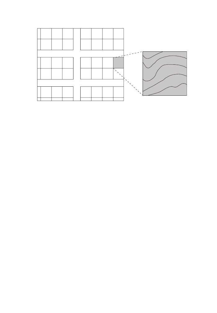
If the database is raster-based, then we have different options, depending on the
sophistication of the system. Let’s have a more detailed look at the right part of
Figure 8. What is displayed here is an elevation dataset. The visual representation
suggests that we have contour lines but this does not necessarily mean that this is the
way the data is actually stored and can hence be queried by. If it is indeed line data,
then the current cursor position would give us nothing because there is no informa-
tion stored for anything in between the lines. If the data is stored as areas (each
plateau of equal elevation forming one area), then we could move around between
any two lines and would always get the same elevation value. Only once we cross a
line would we ‘jump’ to the next higher or lower plateau. Finally, the data could be
4
Spatial Search
Albrecht-3572-Ch-04.qxd 7/13/2007 4:15 PM Page 21
22
KEY CONCEPTS AND TECHNIQUES IN GIS
stored as a raster dataset, but rather than representing thousands of different eleva-
tion values by as many colors, we may make life easier for the computer as well as
for us (interpreting the color values) by displaying similar elevation values with only
one out of say 16 different color values. In this case, the hovering cursor could still
query the underlying pixel and give us the more detailed information that we could
not possibly distinguish by the hue.
This example illustrates another crucial aspect of GIS: the way we store data has
a major impact on what information can be retrieved. We will revisit this theme
repeatedly throughout the book. Basically, data that is not stored, like the area
between lines, cannot simply be queried. It would require rather sophisticated ana-
lytical techniques to interpolate between the lines to come up with a guesstimate for
the elevation when the cursor is between the lines. If, on the other hand, the eleva-
tion is explicitly stored for every location on the screen, then the spatial query is
nothing but a simple lookup.
4.2 Conditional querying
Conditional queries are just one notch up on the level of complication. Within a GIS,
the condition can be either attribute- or geometry-based. To keep it simple and get
the idea across, let’s for now look at attributes only (see Figure 9).
Here, we have a typical excerpt from an attribute table with multiple variables. A
conditional query works like a filter that initially accesses the whole database.
Similar to the way we search for a URL in an Internet search engine, we now pro-
vide the system with all the criteria that have to be fulfilled for us to be interested in
the final presentation of records. Basically, what we are doing is to reject ever more
records until we end up with a manageable number of them. If our query is “Select
the best property that is >40,000m
2
, does not belong to Silma, has tax code ‘B’, and
Parcel# 231-12-687
Owner John
Doe
Zoning A3
Value 179,820
Figure 8
Simple query by location
Albrecht-3572-Ch-04.qxd 7/13/2007 4:15 PM Page 22

SPATIAL SEARCH
23
has soils of high quality”, then we first exclude record #5 because it does not fulfill
the first criterion. Our selection set, after this first step, contains all records but #5.
Next, we exclude record #6 because our query specified that we do not want this
owner. In the third step, we reduce the number of candidates to two because only
records #1 and #3 survived up to here and fulfill the third criterion. In the fourth step,
we are down to just one record, which may now be presented to us either in a win-
dow listing all its attributes or by being highlighted on the map.
Keep in mind that this is a pedagogical example. In a real case, we might end up
with any number of final records, including zero. In that case, our query was overly
restrictive. It depends on the actual application, whether this is something we can
live with or not, and therefore whether we should alter the query. Also, this condi-
tional query is fairly elementary in the way it is phrased. If the GIS database is more
than just a simple table, then the appropriate way to query the database may be to
use one dialect or another of the structured query language SQL.
4.3 The query process
One of the true benefits of a GIS is that we have a choice whether we want to use a
tabular or a map interface for our query. We can even mix and match as part of the
query process. As this book is process-oriented, let’s have a look at the individual
steps. This is particularly important as we are dealing increasingly often with
Internet GIS user interfaces, which are difficult to navigate if the sequence and the
various options on the way are not well understood (see Figure 10).
First, we have to make sure that the data we want to query is actually available.
Usually, there is some table of contents window or a legend that tells us about the
data layers currently loaded. Then, depending on the system, we may have to select
the one data layer we want to query. If we want to find out about soil conditions and
the ‘roads’ layer is active (the terminology may vary a little bit), then our query
result will be empty. Now we have to decide whether we want to use the map or the
tabular interface. In the first instance, we pan around the map and use the identify
Property
Number
Area
M
2
Owner
Tax
Code
Soil
Quality
1
100,000
TULATU
High
High
B
BRAUDO
Medium
A
BRAUDO
Medium
B
ANUNKU
Low
Low
A
ANUNKU
A
SILMA
B
50,000
2
90,000
3
40,800
4
30,200
5
120,200
6
Figure 9
Conditional query or query by (multiple) attributes
Albrecht-3572-Ch-04.qxd 7/13/2007 4:15 PM Page 23

24
KEY CONCEPTS AND TECHNIQUES IN GIS
tool to learn about different restaurants around the hotel we are staying at. In the
second case, we may want to specify ‘Thai cuisine under $40’ to filter the display.
Finally, we may follow the second approach and then make our final decision based
on the visual display of what other features of interest are near the two or three
restaurants depicted.
4.4 Selection
Most of the above examples ended with us selecting one or more records for subse-
quent manipulation or analysis. This is where we move from simple mapping sys-
tems to true GIS. Even the selection process, though, comes at different levels of
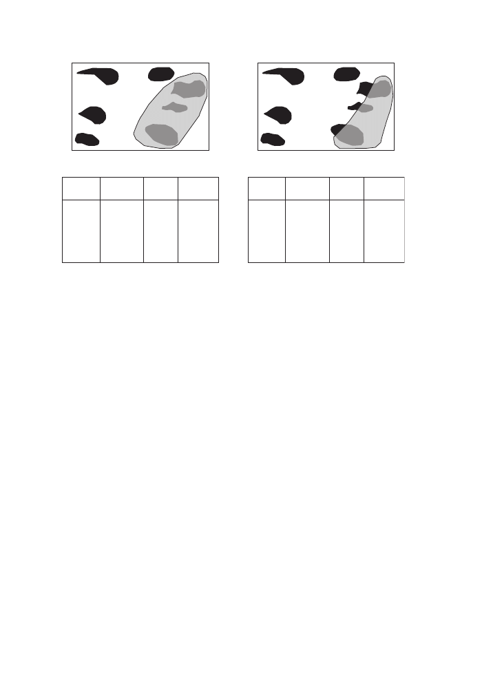
sophistication. Let’s look at Figure 11 for an easy and a complicated example.
In the left part of the figure, our graphical selection neatly encompasses three fea-
tures. In this case, there is no ambiguity – the records for the three features are dis-
played and we can embark on performing our calculations with respect to combined
purchase price or whatever. On the right, our selection area overlaps only partly with
two of the features. The question now is: do we treat the two features as if they got
fully selected or do we work with only those parts that fall within our search area?
If it is the latter, then we have to perform some additional calculations that we will
encounter in the following two chapters.
One aspect that we have glanced over in the above example is that we actually used
one geometry to select some other geometries. Figure 12 is a further illustration of
Command:
List Coverages
Soil
Elevation
Precipitation
Roads
Road Width Length Surface
A
B
C
D
E
8
8
5
5
8
10
5
24
33
31
x–3
x–3
x–5
y–3
y–3
4A
List
Records
List
Fields
5A
5B
3A
3B
Display Database
or
Display Coverage
4B
6B
Zoom
Cursor
Query
Identity:
Road B
Location:
37
°13’22’’S
177
°46’13’’W
1
2
Figure 10
The relationship between spatial and attribute query
Albrecht-3572-Ch-04.qxd 7/13/2007 4:15 PM Page 24
SPATIAL SEARCH
25
the principle. Here, we use a subset of areas (e.g. census areas) to select a subset of
point features such as hospitals. What looks fairly simple on the screen actually
requires quite a number of calculations beneath the surface. We will revisit the topic
in the next chapter.
4.5 Background material: Boolean logic
This topic is not GIS-specific but is necessary background for the next two chapters.
Those who know Boolean logic may merrily jump to the next chapter, the others
should have a sincere look at the following.
Boolean logic was invented by English mathematician George Bool (1815–64)
and underlies almost all our work with computers. Most of us have encountered
Boolean logic in queries using Internet search engines. In essence, his logic can be
described as the kind of mathematics that we can do if we have nothing but zeros
and ones. What made him so famous (after he died) was the simplicity of the rules
to combine those zeros and ones and their powerfulness once they are combined.
The basic three operators in Boolean logic are NOT, OR and AND.
Figure 13 illustrates the effect of the three operators. Let’s assume we have two
GIS layers, one depicting income and the other depicting literacy. Also assume that
the two variables can be in one of two states only, high or low. Then each location
can be a combination of high or low income with high or low literacy. Now we can
look at Figure 13. On the left side we have one particular spatial configuration – not
all that realistic because it’s not usual to have population data in equally sized
spatial units, but it makes it a lot easier to understand the principle. For each area,
we can read the values of the two variables.
Stand
Name
Area
Species
A–3
North
20
Pine
Pine
Mix
10
40
East–1
East–2
C–2
C–2
Stand
Name
Area
Species
A–3
North
10
Pine
Pine
Mix
5
30
East–1
East–2
C–2
C–2
Figure 11
Partial and complete selection of features
Albrecht-3572-Ch-04.qxd 7/13/2007 4:15 PM Page 25

26
KEY CONCEPTS AND TECHNIQUES IN GIS
Now we can query our database and, depending on our use of Boolean operators, we
gain very different insights. In the right half of the figure, we see the results of four
different queries (we get to even more than four different possible outcomes by com-
bining two or more operations). In the first instance, we don’t query about literacy at
all. All we want to make sure is that we reject areas of high income, which leaves us
with the four highlighted areas. The NOT operator is a unary operator – it affects only
the descriptor directly after the operand, in this first instance the income layer.
Point Features
Selected Point Features
Regions
Selected Regions
Figure 13
Simple Boolean logic operations
Figure 12
Using one set of features to select another set
HL
HI
HL
LI
LL
HI
HL
LI
HL
HI
LL
LI
LL
HI
LL
LI
HI
HI
HL
HI
HL
LI
LL
HI
HL
LI
HL
HI
LL
LI
LL
HI
LL
LI
HI
HI
HL
HI
HL
LI
LL
HI
HL
LI
HL
HI
LL
LI
LL
HI
LL
LI
HI
HI
HL
HI
HL
LI
LL
HI
HL
LI
HL
HI
LL
LI
LL
HI
LL
LI
HI
HI
HL
HI
HL
LI
LL
HI
HL
LI
HL
HI
LL
LI
LL
HI
LL
LI
HI
HI
HL not HI
HL: High Literacy
LL: Low Literacy
HI: High Income
LI: Low Income
HL and HI
HL or HI
Not HI
Albrecht-3572-Ch-04.qxd 7/13/2007 4:15 PM Page 26

Next, look at the OR operand. Translated into plain English, OR means ‘one or
the other, I don’t care which one’. This is in effect an easy-going operand, where
only one of the two conditions needs to be fulfilled, and if both are true then the
better. So, no matter whether we look at income or literacy, as long as either one (or
both) is high, the area gets selected. OR operations always result in a maximum
number of items to be selected.
Somewhat contrary to the way the word is used in everyday English, AND does
not give us the combination of two criteria but only those records that fulfill both
conditions. So in our case, only those areas that have both high literacy and high
income at the same time are selected. In effect, the AND operand acts like a strong
filter. We saw this above in the section on conditional queries, where all conditions
had to be fulfilled.
The last example illustrates that we can combine Boolean operations. Here we
look for all areas that have a high literacy rate but not high income. It is a combina-
tion of our first example (NOT HI) with the AND operand. The result becomes clear
if we rearrange the query to state NOT HI AND HL. We say that AND and OR are
binary operands, which means they require one descriptor on the left and one on the
right side. As in regular algebra, parentheses () can be used to specify the sequence
in which the statement should be interpreted. If there are no parentheses, then NOT
precedes (overrides) the other two.
SPATIAL SEARCH
27
Albrecht-3572-Ch-04.qxd 7/13/2007 4:15 PM Page 27

Albrecht-3572-Ch-04.qxd 7/13/2007 4:15 PM Page 28

Spatial relationships are one of the main reasons why one would want to use a GIS.
Many of the cartographic characteristics of a GIS can be implemented with a draw-
ing program, while the repository function of large spatial databases is often taken
care of by traditional database management systems. It is the explicit storage of
spatial relationships and/or their analysis based on geometric reasoning that distin-
guishes GIS from the rest of the pack.
We ended the last chapter with a select-by-location operation, which already
makes use of a derived relationship between areas and points that lay either inside
or outside these areas. Before we embark on a discussion of many other important
spatial relationships, we should insert a little interlude in the form of the spatial data-
base operation ‘recode’. Functionally, and from the perspective of typical GIS usage,
this operation sits in between simple spatial queries and more advanced analytical
functions that result in new data.
5.1 Recoding
Recoding is an operation that is usually applied when the contents of a database have
become confusingly complicated; as such it is used to simplify (our view of) the
database. Soil maps, such as the one depicted in Figure 14, are a perfect example of
that. Ten different soil types may be of interest to the pedologist, but for most
others it is sufficient to know whether the ground is stable enough to build a high-
rise or dense enough to prevent groundwater leakages. In that case, we would like to
aggregate the highly detailed information contained in a soils database and recoding
is the way to do it.
Figure 15 is a stylized version of the previous soil map and illustrates how the
combination of attributes also leads to a combination of geometries. We will make
use of this side effect in the next chapter, when, as a result of combining spatial data,
we have more geometries than we would like. Alternatively, we could use the recod-
ing operation not as much to simplify our view of the database but to reflect a par-
ticular interpretation of the data. A simple application of this is given in Figure 16,
where we simplify a complex map to a binary suitable/non-suitable for agricultural
purposes.
A more complicated (and interesting) version of the same procedure is given in
Figure 17. Here, we recode a complex landcover map by first extracting all different
vegetation types and then recombine these to form a new dataset containing all kinds
of vegetation and nothing but vegetation. In both of these examples, we are creating
5
Spatial Relationships
Albrecht-3572-Ch-05.qxd 7/13/2007 4:15 PM Page 29

30
KEY CONCEPTS AND TECHNIQUES IN GIS
Figure 14
Typical soil map
Typical soil map
Recoded soil map
Simplified map with 10
different soil types
Attribute
Code
Soil
Type
4
4
1
3
2
10
10
9
6
6
7
5
7
9
8
8
1
A1Z
A3X
A2Z
A1H
B1H
B3X
B1X
C3H
C2H
C2X
2
3
4
5
6
7
8
9
10
Attribute
Recode
New
Soil
1
1
A
B
C
2
3
2
3
Figure 15
Recoding as simplification
Albrecht-3572-Ch-05.qxd 7/13/2007 4:15 PM Page 30
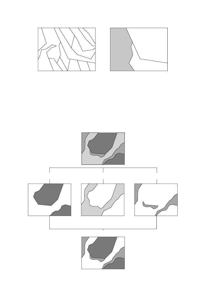
SPATIAL RELATIONSHIPS
31
Soils Before Recoding
Agricultural Soils – A
Agricultural Soils
Non-agricultural Soils – B, C
Recode:
Figure 16
Recoding as a filter operation
Land Cover
Open
Brush
Forest
Vegetation
Figure 17
Recoding to derive new information
Albrecht-3572-Ch-05.qxd 7/13/2007 4:15 PM Page 31

32
KEY CONCEPTS AND TECHNIQUES IN GIS
new data based on a new interpretation of already existing data. There is no category
‘vegetation’ in the original landcover dataset. We will revisit the topic of creating new
data rather than just querying existing data in the next chapter on combining data. This
sneak preview is an indicator of the split personality of the recoding operation; it could
be interpreted as a mere data maintenance operation or as an analytical one.
One intriguing aspect that comes to mind when one looks at Figures 16 and 17 is
that we immediately try to discern patterns in the distribution of selected areas.
Spatial relationships can be studied quantitatively or qualitatively. The former will
be the subject of Chapter 10, while the latter is addressed in the following sections.
Features are defined by their boundaries. On the qualitative side, we can therefore
distinguish between two types of spatial relationship, one where we look at how
individual coordinates are combined to form feature boundaries and the other where
we look at the spatial relationships among features.
5.2 Relationships between measurements
As discussed in Chapter 2, all locational references can be reduced to one or more
coordinates, which are either measured or interpolated. It is important to remind our-
selves that we are talking about the data in our geographic databases, not the geome-
tries that are used to visualize the geographic data, which may be the same but most
likely are not. If you are unsure about this topic, please revisit Chapter 2.
Next, we need to distinguish between the object-centered and the field-based rep-
resentations of geographic information (see also Chapter 1). The latter does not have
any feature representation, so the spatial relationships are reduced to those of the
respective positions of pixels to each other. This then is very straightforward, as we
have only a very limited number of scenarios, as depicted in Figure 18:
•
Cell boundaries can touch each other.
•
Cell corners can touch each other.
•
Cells don’t touch each other at all.
•
Cells relate to each other not within a layer but across (vertically).
We will revisit the cell relationships in Chapter 8, when we look at the analytical
capabilities of raster GIS – which are entirely based on the simplicity of their spatial
relationships.
Features, on the other hand, are defined by their boundaries. We distinguish zero-
through 3-dimensional simple features from their complex counterparts (see Figure
19). One and the same node, edge or area can be shared by any number of higher-
dimensional features. Older GIS consisted of tables of points, lines and areas, which
all consisted of pointers to the respective lower-dimensional tables (see Figure 20).
Modern systems store the nodes of higher-dimensional features redundantly and use
topological rules (see next section) to enforce database integrity. Complex features
consist of multiple disconnected geometries that are treated as one uniform object.
Albrecht-3572-Ch-05.qxd 7/13/2007 4:15 PM Page 32

SPATIAL RELATIONSHIPS
33
No touching
at all
No relationship within,
but across layers
Corners touch
each other
Boundaries touch
each other
Figure 18
Four possible spatial relationships in a pixel world
Figure 19
Simple (top row) and complex (bottom row) geometries
Albrecht-3572-Ch-05.qxd 7/13/2007 4:15 PM Page 33
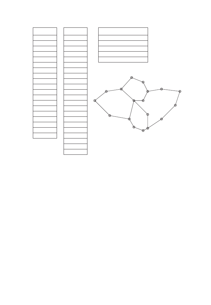
34
KEY CONCEPTS AND TECHNIQUES IN GIS
Networks form an extra category of relationships between measurements. Similar
to one-dimensional features, the connections between any two nodes are more
abstract. In the world of features, we assume a spatial relationship, when two ele-
ments have the same coordinate. In networks, the default is no relationship, unless
it has been explicitly stored as a node attribute. A network is understood as a graph
whose lines may or may not intersect even when they visually do. The technical term
for this is non-planarity, which means that although we draw the network on a flat
plane, the intersecting lines may actually mean to be at different levels. A subway
map would be a practical example of that; if the lines intersect without a station sym-
bol (a node) then there is no connectivity, which in turn means that passengers can-
not switch from one line to the other (see Figure 21). The qualitative spatial
relationship is hence one of connectedness – whether a node is reachable or not.
5.3 Relationships between features
The qualitative spatial relationship between features is again described in a form of
connectedness called topology. Topology is the branch of mathematics that deals
with persistence of relationships, no matter how much we contort the objects of
Node table
Line table
Area table
01 07,30
02 12,35
03 15,22
04 20,37
05 25,20
06 28,30
01 01,02
02 02,04
03 04,07
04 07,11
05 11,12
06 12,16
01 1,2,17,16,14,15
02 3,4,5,19,18,17
03 6,7,8,9,10,21,20,18,19
04 20,21,11,12,13,16
ID x,y
ID from to
ID lines
07 16,18
08 18,17
09 17,15
10 15,14
11 14,09
12 09,08
13 08,05
14 05,03
15 03,01
16 05,06
17 06,04
18 06,10
19 10,12
20 10,13
21 13,14
07 27,42
08 28,15
09 32,14
10 32,30
11 32,40
12 35,35
13 35,22
14 35,15
15 42,20
16 42,37
17 50,28
18 52,35
1
2
3
4
5
6
7
8
9
10
11
12
13
14
15
16
17
18
A
B
C
D
E
F
G
H
I
K
L
M
N
19
20
21
O
P
R
S
Q
Figure 20
Pointer structure between tables of feature geometries
Albrecht-3572-Ch-05.qxd 7/13/2007 4:15 PM Page 34
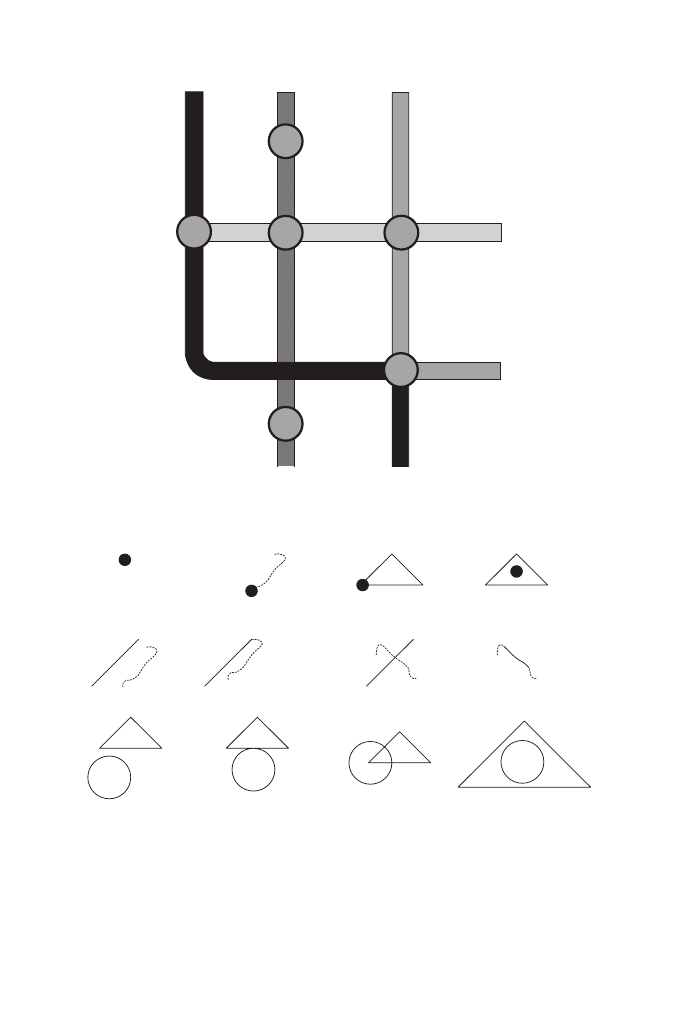
SPATIAL RELATIONSHIPS
35
interest, short of cutting them up. We distinguish between containment, intersecting,
touching, and no relationship whatsoever, and do so for the relationships across a
range of dimensionalities. We hence have all possible combinations of the above
relationships among and between points, lines, areas and volumes (Egenhofer 1993).
18th St
6th Ave
W 4th St
Christopher St
Figure 21
Part of the New York subway system
Figure 22
Topological relationships between features
Albrecht-3572-Ch-05.qxd 7/13/2007 4:15 PM Page 35

36
KEY CONCEPTS AND TECHNIQUES IN GIS
Figure 22 lists a selection of such topological relationships. Volumes have been
written about what are the mathematically distinguishable qualitative relationships,
how they relate to quantitative measures, and whether we even have names for them
in different human languages. In English, for instance, we use verbs such as touch,
border, intersect, overlap and contain, to describe the relationships depicted in
Figure 22.
The use of topological rules has proven to be a very useful instrument for check-
ing the consistency of a GIS database. Until recently, GIS could store only one type
of geometry per feature class. Spatial relationships within one and the same feature
class can be encoded as part of the data structure, which imposes additional con-
straints on the data organization and helps to check for database consistency. If these
rules are applied across feature classes, then we have to (a) perform a topology check
by at least temporarily combining spatial features, and (b) store these in an extra
table that is associated with a group of feature classes. We will revisit this topic in
the next chapter about combining spatial data.
Albrecht-3572-Ch-05.qxd 7/13/2007 4:15 PM Page 36

As mentioned in the previous chapter, many spatial relationships are difficult to
derive or even describe. Rather than storing all possible relationships between all
features of a database, we can use GIS operations to answer specific questions about
the spatial relationships among our features of interest. This is not only far more effi-
cient but also gives us more freedom, because we can determine on the fly what
pieces of data we want to relate to each other – and in the age of the Internet, these
pieces may even be distributed across the world.
This chapter deals with two families of GIS operations that in practice make up
some 75–80% of all analytical GIS operations. Overlay is the quintessential GIS
operation that seems to define a GIS. If a software package can perform overlay
operations, then it is indeed a GIS and not a mere CAD or cartography program. The
poor cousin is the buffer operation, which always seems to be mentioned second.
Both are actually place-holders for a number of different operations, but we will
discuss this in detail in the following.
6.1 Overlay
In the recoding section of the last chapter, we saw how tightly linked attributes and
geometries are. By recombining attributes we automatically changed the graphical
representation as well. However, when we look at it from the perspective of lines
store in our database (see Figure 20), the recoding operation did not create any new
geometries. This changes now with the group of overlay operations. Let’s look at
Figure 23 to see what happens to geometries and attributes in an overlay operation.
For pedagogical reasons, we use very simple geometries and only two layers of
binary data. This is extremely unrealistic but helps us to get the principle across. We
will look at more realistic examples later on.
The figure shows a number of important aspects of the overlay operation. We have
two or more input feature classes and one (new) output feature class. The geometries
of the two input layers are most likely to be different; that is, they do not have to
come from the same provider and do not have to have anything in common other
than the general extent (it does not make sense to overlay data in South America with
other data from Africa). Also observe that the first feature class has no attributes
describing vegetation, while the second has none describing soils. The overlay oper-
ation depicted here looks for coincidences at the same location. In other words, for
any given location, it looks what information there is in one feature class, then in the
6
Combining Spatial Data
Albrecht-3572-Ch-06.qxd 7/13/2007 5:08 PM Page 37

38
KEY CONCEPTS AND TECHNIQUES IN GIS
other feature class, and then it combines the two in the output dataset. The geome-
tries of the output dataset did not exist before. We really create completely new data.
We used this notion of coincidence earlier when we looked at some of the more
advanced spatial search functions. Figure 24 is a case in point.
Input
Feature Class 1
Input
Feature Class 1
Output
Feature Class 3
+
=
Polygon
Type
Size
Polygon
Type
Size
Polygon
Type
Size
1
Clay
2
Sand
2
2
A
1A
1
1
1
1
Clay Grass
Sand Grass
Sand Trees
Clay Trees
2A
1B
2B
Grass
2
2
Trees
B
Soils
Vegetation
C
LAY
1
2
S
AND
G
RASS
2A
1A
2B
1B
T
REES
A
B
Figure 23
Schematics of a polygon overlay operation
Soils
Which soils occur in County C?
Coincidence view
Counties
A
B
C
D
E
Figure 24
Overlay as a coincidence function
Albrecht-3572-Ch-06.qxd 7/13/2007 5:08 PM Page 38
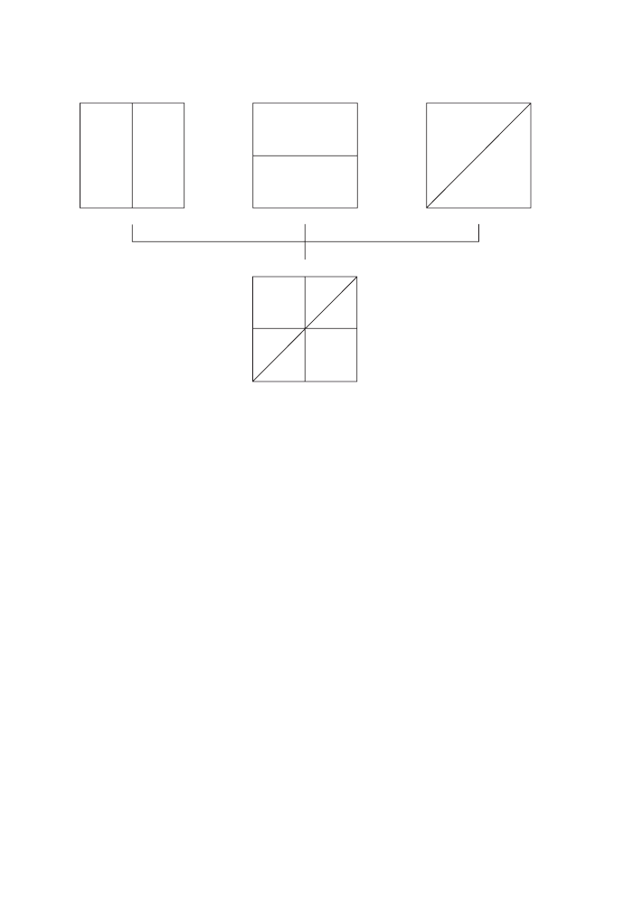
COMBINING SPATIAL DATA
39
The question ‘Which soils occur in county C?’ appears to be a simple spatial
search function. However, what actually happens here is that we overlay the two fea-
ture classes and then look for those parts of the soils feature class that fall within the
polygon that marks county C in the counties feature class. In Chapter 4, we did not
have an answer to how to deal with those soil polygons that lie only partially within
county C. Now, we applied the overlay operation like a cookie cutter and created
several new pieces of data. When you look back at Figure 23, you see that there is
quite a lot happening here. New files or at least tables get created, new geometries
have to be calculated, new connections between attributes and geometries have to
be formed and maintained. This may seem like a lot for a simple spatial search
operation – and it is! Keep this in mind, the next time you wait impatiently for the
result of your spatial search.
What we did in Figure 24 was to overlay one layer of areal features with another
one. A slightly more complicated (realistic) example is depicted in Figure 25. Here
we are using three input layers and possibly some weighting scheme to calculate
agricultural yield potential. Going beyond the pure area-on-area situation, we could
just as well overlay areal with point or line feature classes, for example to determine
which historic site is in what administrative unit or to ascertain all the countries that
the river Nile is flowing through. We could even overlay point and line feature
classes to learn whether the Christopher St subway station is on the red or the blue
line (see Figure 21). In each of these cases we make use of the topological relation-
ships between all the features involved.
Soil Type
Crop Type
Yield Potential
1AX
1BX
1BY
2BY
2AY
2AX
Farming Practice
A
B
1
2
Y
X
+
+
Figure 25
Overlay with multiple input layers
Albrecht-3572-Ch-06.qxd 7/13/2007 5:08 PM Page 39

40
KEY CONCEPTS AND TECHNIQUES IN GIS
6.2 Spatial Boolean logic
In Chapter 4, we looked briefly at Boolean logic as the foundation for general com-
puting. You may recall that the three basic Boolean operators were NOT, AND and
OR. In Chapter 4, we used them to form query strings to retrieve records from attrib-
ute tables. The same operators are also applicable to the combination of geometries;
and in the same way that the use of these operators resulted in very different outputs,
the application of NOT, AND and OR has completely different effects on the com-
bination (or overlay) of layer geometries.
Figure 26 illustrates the effect of the different operands in a single overlay opera-
tion. This is why we referred to overlay as a group of functions. Figure 26 is possi-
bly the most important in this book. It is not entirely easy to digest the information
provided here and the reader is invited to spend some time studying each of the sit-
uations depicted. Again, for pedagogical reasons, there are only two layers with only
one feature each. In reality, the calculations are repeated thousands of times when
we overlay two geographic datasets. What is depicted here is the resulting geometry
only. As in the example of Figure 23 above, all the attributes from all the input
layers are passed on to the output layer.
Depending on whether we use one or two Boolean operators and how we relate
them to the operands, we get six very different outcomes. Clearly one overlay is not
the same as the other. At the risk of sounding overbearing, this really is a very impor-
tant figure to study. GIS analysis is dependent on the user understanding what is
All but A and B
Everything not A or B
Separate identities
for each segment
Any A that does
not include B
Union levels
A not B
Intersect A and B
Coincidence A and B
A or B but not both
Any part A or B
Not intersect
Union A or B
A
+
B
Figure 26
Spatial Boolean logic
Albrecht-3572-Ch-06.qxd 7/13/2007 5:08 PM Page 40

COMBINING SPATIAL DATA
41
happening here and being able to instruct whatever system is employed to perform
the correct overlay operation.
The relative success of the overlay operations can be attributed to their cognitive
consonance with the way we detect spatial patterns. Overlays are instrumental in
answering questions like ‘What else can be observed at this location?’, or ‘How often
do we find woods and bison at the same place?’.
6.3 Buffers
Compared to overlay, the buffer operation is more quantitative if not analytical. And
while, at least in a raster-based system, we could conceive of overlay as a pure data-
base operation, buffering is as spatial as it gets. Typically, a buffer operation creates
a new area around our object of interest – although we will see exotic exceptions
from this rule. The buffer operation takes two parameters: a buffer distance and
the object around which the buffer is to be created. The result can be observed in
Figure 27.
A classical, though not GIS-based, example of a buffer operation can be found in
every larger furniture store. You will invariably find some stylized or real topo-
graphic map with concentric rings usually drawn with a felt pen that center on the
location of the store or their storage facility. The rings mark the price that the store
charges for the delivery of their furniture. It is crude but surprisingly functional.
Regardless of the dimension of the input feature class (point, line or polygon), the
result of a regular buffer operation is always an area. Sample applications for points
would be no-fly zones around nuclear power plants, and for lines noise buffers
around highways. The buffer distance is usually applied to the outer boundary of the
object to be buffered. If features are closer to each other than the buffer distance
between them, then the newly created buffer areas merge – as can be seen for the
two right-most groups of points in Figure 27.
There are a few interesting exceptions to the general idea of buffers. One is the
notion of inward buffers, which by its nature can only be applied to one- or higher-
dimensional features. A practical example would be to define the core of an ecological
Original Points
Buffered Points
Dissolved Buffers
Figure 27
The buffer operation in principle
Albrecht-3572-Ch-06.qxd 7/13/2007 5:08 PM Page 41
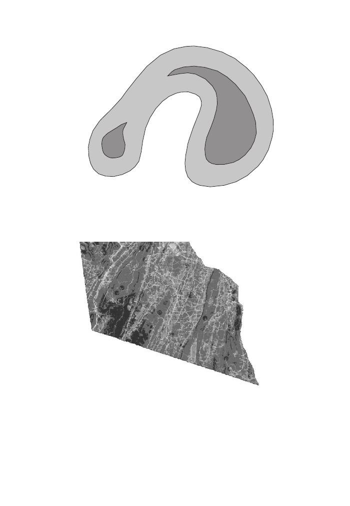
42
KEY CONCEPTS AND TECHNIQUES IN GIS
reserve (see Figure 28). A combination of the regular and the inverse buffer applied
simultaneously to all features of interest is called a corridor function (see Figure 29).
Finally, within a street network, the buffer operation can be applied along the edges
(a one-dimensional buffer) rather than the often applied but useless as-the-crow-flies
circular buffer. We will revisit this in the next chapter.
Core
Figure 28
Inward or inverse buffer
Figure 29
Corridor function
Albrecht-3572-Ch-06.qxd 7/13/2007 5:08 PM Page 42

COMBINING SPATIAL DATA
43
6.4 Buffering in spatial search
A few paragraphs above we saw how overlay underlies some of the (not overtly)
more complicated spatial search operations. The same holds true for buffering.
Conceptually, buffers are in this case used as a form of neighborhood. ‘Find all
customers within ZIP code 123’ is an overlay operation, but ‘Find all customers in a
radius of 5 miles’ is a buffer operation. Buffers are often used as an intermediate
select, where we use the result of the buffer operation in subsequent analysis (see
next section).
6.5 Combining operations
If the above statement that buffers and overlays make up in practice some 75% of
all analytical GIS functionality is true, then how is it that GIS has become such an
important genre of software? The solution to this paradox lies in the fact that opera-
tions can be concatenated to form workflows. The following is an example from a
major flood in Mozambique in 2000 (see Figure 30).
Input layers
Roads
Towns
River
Directly affected;
under water
Indirectly affected;
dry but cut off
Not affected at all
Overlay and buffer
Overlay
Identification of
indirectly affected
towns
Figure 30
Surprise effects of buffering affecting towns outside a flood zone
Albrecht-3572-Ch-06.qxd 7/13/2007 5:08 PM Page 43

44
KEY CONCEPTS AND TECHNIQUES IN GIS
We start out with three input layers – towns, roads and hydrology. The first step
is to buffer the hydrology layer to identify flood zones (this makes sense only in
coastal plains, such as was the case with the Southern African floods in 2000). Step
two is to overlay the township layer with the flood layer to identify those towns that
are directly affected. Parallel to this, an overlay of the roads layer with the flood
layer selects those roads that have become impassable. A final overlay of the impass-
able roads layer with the towns helps us to identify the towns that are indirectly
affected – that is, not flooded but cut off because none of the roads to these towns is
passable. Figure 30 is only a small subset of the area that was affected in 2000.
6.6 Thiessen polygons
A special form of buffer is hidden behind a function that is called a Thiessen poly-
gon (pronounced the German way as ‘ee’) or Voronoi diagram. Originally, these
functions had been developed in the context of graph theory and applied to GIS
based on triangulated irregular networks (TINs), which we will discuss in Chapter
9. It is introduced here as a buffer operation because conceptually what happens is
that each of the points of the input layer is simultaneously buffered with ever-
increasing buffer size. Wherever the buffers hit upon each other, a ‘cease line’ is cre-
ated until no buffer can increase any more. The result is depicted in Figure 31.
Figure 31
Thiessen polygons
Each location within the newly created areas is closer to the originating point than
to any other one. This makes Thiessen polygons an ideal tool for allocation studies,
which we will study in detail in the next chapter.
Albrecht-3572-Ch-06.qxd 7/13/2007 5:08 PM Page 44

Among the main reasons for wanting to use a GIS are (1) finding a location, (2) finding
the best way to get to that location, (3) finding the best location to do whatever our
business is, and (4) optimizing the use of our limited resources to conduct our
business. The first question has been answered at varying levels of complexity in the
earlier chapters. Now I want to address the other three questions.
General GIS textbooks usually direct the reader to answer these questions by
using the third and so far neglected form of GIS data structure, the network GIS.
This is, however, slightly misleading as we could just as well use map algebra
(Chapter 8), and some of the more advanced regional science models would even
use data aggregated to polygons (although here the shape of the polygons and hence
much of the reason why we would use vector GIS is not considered). The following
notes are more about concepts; the actual procedures in raster or in network GIS
would differ considerably from each other. But that is an implementation issue and
should not be of immediate concern to the end user.
7.1 The best way
Finding the best way to a particular location is usually referred to as shortest-path
analysis. But that is shorthand for a larger group of operations, which we will look
at here. To determine the best way one needs at a minimum an origin and a desti-
nation. On a featureless flat plain, the direct line between these two locations would
mark the best way. In the real world, though, we have geography interfering with
this simple geometric view. Even if we limit ourselves to just the shortest distance,
we tend to stay on streets (where available), don’t walk through walls, and don’t
want to get stuck in a traffic jam. Often, we have other criteria but pure distance that
determine which route we choose: familiarity, scenery, opportunity to get some
other business done on the way, and so on. Finally, we typically are not the only
ones to embark on a journey, say from home to work. Our decisions, our choice of
what is the best way, are influenced by what other people are doing, and they are
time-dependent. An optimal route in the morning may not easily be traced back in
the evening. In most general terms, what we are trying to accomplish with our best-
way analysis is to model the flows of commodities, people, capital or information
over space (Reggiani 2001). How, then, can all these issues be addressed in a GIS,
and how does all this get implemented?
A beginning is to describe the origin and the target. This could be done in the
form of two coordinate pairs, or a relative position given by distance and direction
7
Location–Allocation
Albrecht-3572-Ch-07.qxd 7/13/2007 4:16 PM Page 45

46
KEY CONCEPTS AND TECHNIQUES IN GIS
from an origin. Either location can be imbued with resources in the widest sense,
possibly better described as push and pull factors. Assuming for a moment that the
origin is a point (node, centroid, pixel), we can run a wide range of calculations on
the attributes of that point to determine what factors make the target more desirable
than our origin and what resources to use to get there. The same is true for any point
in between that we might visit or want to avoid. Finally, we have to decide how we
want to travel. There may be a constraining geometry underlying our geography. In
the field view perspective we could investigate all locations within our view shed,
whereas in a network we would be constrained by the links between the nodes.
These links usually have a set of attributes of their own, determining speed, capac-
ity (remember, we are unlikely to be the only ones with the wish to travel), or mode
of transport. In a raster GIS, the attributes for links and nodes are combined at each
pixel, which actually makes it easier to deal with hybrid functionality such as turns.
Turn tables are a special class of attribute table that permit or prevent us from chang-
ing direction; they can also be used to switch modes of transportation. Each pixel,
node or link could have its own schedule or a link to a big central time table that
determines the local behavior at any given time in the modeling scenario.
The task is then to determine the best way among all the options outlined above.
Two coordinate pairs and a straight line between them rarely describes our real
world problem adequately (we would not need a GIS for that). The full implemen-
tation of all of the above options is as of writing this book just being tested for a few
mid-sized cities. Just to assemble all the data (before even embarking on developing
the routing algorithms) is a major challenge. Given the large number of options, we
are faced with an optimization problem. The implementation is usually based on
graph theoretical constructs (forward star search, Dijkstra algorithm) and will not be
covered here. But conceptually, the relationship between origins and targets is based
on the gravity model, which we will look at in the following section.
7.2 Gravity model
In the above section, we referred to the resources that we have available and talked
about the push and pull of every point. This vocabulary is borrowed from a naive
model of physics going all the way back to Isaac Newton. Locations influence each
other in a similar way that planets do in a solar system. Each variable exerts a field
of influence around its center and that field is modeled using the same equations that
were employed in mechanics. This intellectual source has provided lots of ammuni-
tion for social scientists who thought the analogy to be too crude. But modern appli-
cations of the gravity model in location–allocation models are as similar to Newton’s
role model as a GPS receiver to a compass.
The gravity model in spatial analysis is the inductive formalization of Tobler’s
First Law (see Chapter 10). Mathematically, we refer to a distance–decay function,
which in Newton’s case was one over the square of distance but in spatial analysis
can be a wide range of functions. By way of example, $2 may get me 50 km away
Albrecht-3572-Ch-07.qxd 7/13/2007 4:16 PM Page 46
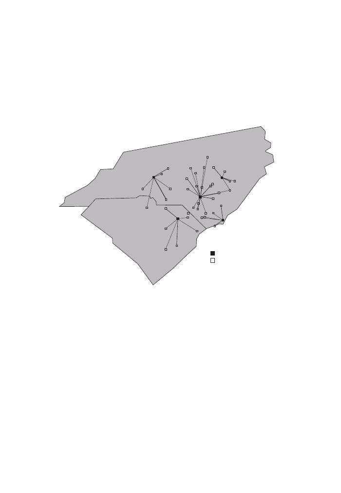
LOCATION–ALLOCATION
47
from the central station in New York, 20 km in Hamburg, Germany, and nowhere
in Detroit if my mode of transport is a subway train. We can now associate fields of
influence based on a number of different metrics with each location in our dataset
(see Figure 32). Sometimes they act as a resource as in our fare example, sometimes
they act as an attractor that determines how far we are willing to access a certain
resource (school, hospital, etc.). Sometimes they may even act as a distracter, an
area that we don’t want to get too close to (nuclear power plants, prisons, predators).
North Carolina
Rocky Mount
Fayetteville
Wilmington
Statesville
Florence
South Carolina
Sinks
Sources
Figure 32
Areas of influence determining the reach of gravitational pull
This push and pull across all known locations of a study area forms the basis for
answering the next question, finding the optimal location or site for a particular
resource, be it a new fire station or a coffee shop. The next section will describe the
concepts behind location modeling.
7.3 Location modeling
Finding an optimal location has been the goal of much research in business schools
and can be traced all the way back to nineteenth and early twentieth century schol-
ars such as von Thünen, Weber and Christaller. The idea of the gravity model applies
to all of them (see Figures 33–35), albeit in increasingly complicated ways. Von
Thünen worked on an isolated agricultural town. Weber postulated a simple triangle
of resource, manufacturer and market location. Christaller expanded this view into a
whole network of spheres of influence.
Albrecht-3572-Ch-07.qxd 7/13/2007 4:16 PM Page 47
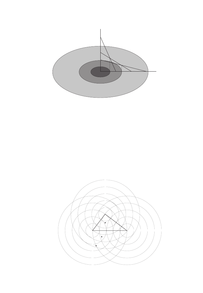
48
KEY CONCEPTS AND TECHNIQUES IN GIS
In the previous chapter, if we had wanted to find an optimal location, we would
have used a combination of buffer and overlay operations to derive the set of loca-
tions, whose attribute combination and spatial characteristics fulfill a chosen crite-
rion. While the buffer operation lends a bit of spatial optimization, the procedure
(common as it is as a pedagogical example) is limited to static representations of
territorial characteristics. Location modeling has a more human-centered approach
and captures flows rather than static attributes, making it much more interesting. It
tries to mimic human decision choices at every known location (node, cell or area).
Weber’s triangle (Figure 34) is particularly illustrative of the dynamic character of
the weights pulling our target over space.
R
A
B
C
A
B
C
K
Z
I
II
III
Zone 1
Zone 2
Zone 3
Figure 33
Von Thünen’s agricultural zones around a market
M = Raw material
K = Consumer
P = Production
L = Labor
M
2
M
1
L
1
L
2
P
K
1
2
3
4
5
5
4
3
2
1
1
2
3
4
5
Figure 34
Weber’s triangle
Albrecht-3572-Ch-07.qxd 7/13/2007 4:16 PM Page 48
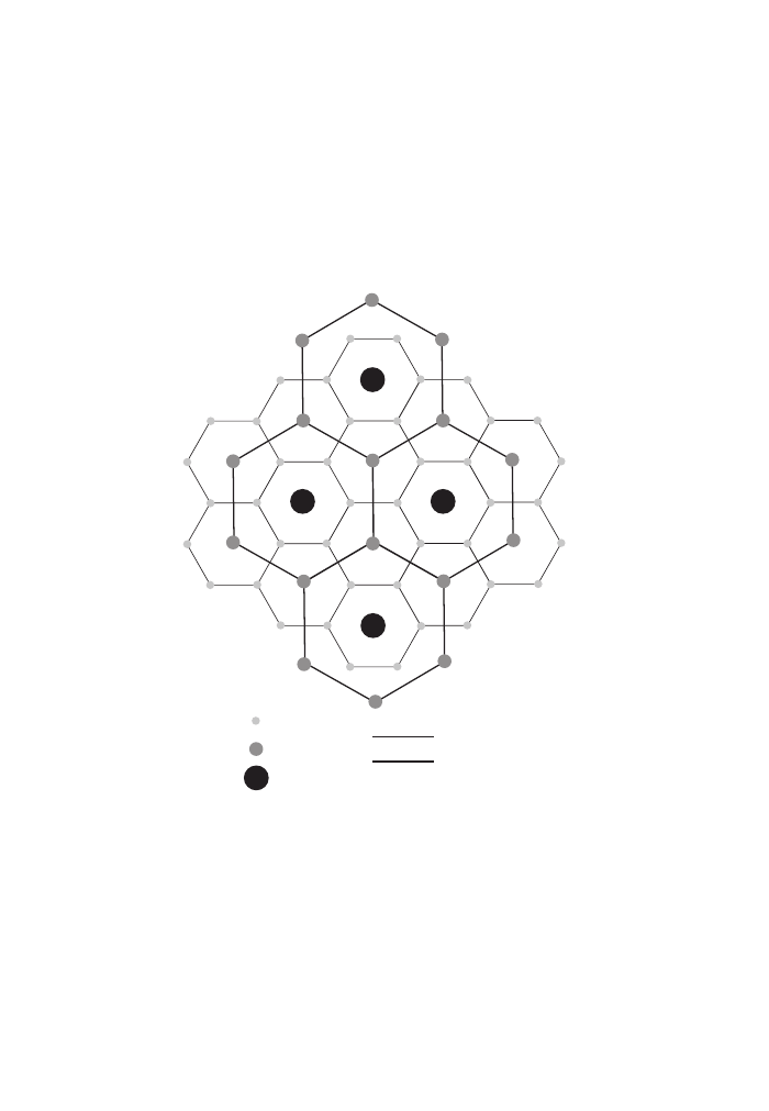
LOCATION–ALLOCATION
49
Two additions to this image drive the analogy home. Rather than having a plane
surface, we model the weights pulling our optimal center across some rugged terrain.
Each hill and peak marks push factors or locations we want to avoid. The number of
weights is equivalent to the number of locations that we assume to have an influence
over our optimal target site. The weights themselves finally consist of as many
criteria given as much weight as we wish to apply. The weights could even vary
depending on time of day, or season, or real-time sensor readings. The latter would
then be an example for the placement of sentinels in a public safety scenario.
Central Place
Theory
Boundaries
Village
Town
City
Figure 35
Christaller’s Central Place theory
The implementation of such a system of gravity models is fairly straightforward
for a raster model (as we will see in the discussion of zonal operations in the fol-
lowing chapter) or a network model (particularly if our commodities are shipped
along given routes). For a system of regions interacting with each other, the imple-
mentation is traditionally less feature-based. Instead, large input–output tables
representing the flows from each area to each other area are used in what is called a
flow matrix (see Figure 36). The geometry of each of these areas is neglected and
the flows are aggregated to one in each direction across a boundary. Traditionally
employed in regional science applications, the complications of geometry are
Albrecht-3572-Ch-07.qxd 7/13/2007 4:16 PM Page 49

50
KEY CONCEPTS AND TECHNIQUES IN GIS
overridden by the large number of variables (weights) that are pulling our target cell
across the matrix.
7.4 Allocation modeling
All of the above so far assumed that there is only one target location that we either
want to reach or place. If this decision has already been made (by us and/or our com-
petitors) then the question arises as to what is the next best location. As in the
statistical urn game, we may want to pursue this question with or without the option
of moving already existing sites. And finally, we may want to find out when the rate
of diminishing returns means that we have saturated the market (the term ‘market’
is here to be seen in a very wide sense; we could talk about placement of policemen,
expensive instruments, any non-ubiquitous item). Allocation models are the domain
of optimization theory and operations research, and the spatial sciences have not
made many inroads into these fields. In the course of this chapter, the problems
tackled and the required toolset have grown ever bigger. Allocation models, if they
are supposed to show any resemblance with reality, are enormously complicated
and require huge amounts of data – which often does not exist (Alonso 1978). The
methods discussed in Chapter 11, in particular a combination of genetic algorithms,
neural networks and agent-based modeling systems, may be employed to address
these questions in the future.
The discussion above illustrates how models quickly become very complicated
when we try to deal with a point, line and polygon representation of geographic
phenomena. Modelers in the natural sciences did not abandon the notion of space to
the degree that regional scientists do and turned their back on spatial entities rather
than space itself. In other words, they embraced the field perspective, which is
computationally a lot simpler and gave them the freedom to develop a plethora of
advanced spatial modeling tools, which we will discuss in the next chapter.
Figure 36
Origin-destination matrix
From
Zone 1
Zone 2
Zone 3
Row sums
Zone 1
27
4
16
47
Zone 2
9
23
4
36
Zone 3
0
6
20
26
Column sums
36
33
40
109
To Destinations
Albrecht-3572-Ch-07.qxd 7/13/2007 4:16 PM Page 50

This chapter introduces the most powerful analytical toolset that we have in GIS.
Map algebra is inherently raster-based and therefore not often taught in introductory
GIS courses, except for applications in resource management. Traditional vector-
based GIS basically knows the buffer and overlay operations we encountered
in Chapter 6. The few systems that can handle network data then add the location–
allocation functionality we encountered in Chapter 7. All of that pales in compari-
son to the possibilities provided by map algebra, and this chapter can really only
give an introduction. Please check out the list of suggested readings at the end of this
chapter.
Map Algebra was invented by a chap called Dana Tomlin as part of his PhD
thesis. He published his thesis in 1990 under the very unfortunate title of
Cartographic Modeling and both names are used synonymously. His book (Tomlin
1990) deserves all the accolades that it received, but the title is really misleading, as
the techniques compiled in it have little if anything to do with cartography.
The term ‘map algebra’ is apt because it describes arithmetic on cells, groups of
cells, or whole feature classes in form of equations. Every map algebra expression has
the form <output
=
function(input)>. The function can be unary (applying to only one
operand), binary (combining two operands as in the elementary arithmetic functions
plus, minus, multiply and divide), or n-ary, that is applying to many operands at once.
We distinguish map algebra operations by their spatial scope; local functions
operate on one cell at a time, neighborhood functions apply to cells in the immedi-
ate vicinity, zonal functions apply to all cells of the same value, and global functions
apply to all cells of a layer/feature class. In spite of the scope, all map algebra func-
tions work on a cell-by-cell basis. The scope only determines how many other cells
the function takes into consideration, while calculating the output value for the cell
it currently operates on (see Figure 37). However, before we get into the details of
map algebra functions, we have to have a look at how raster GIS data is organized.
8.1 Raster GIS
Raster datasets can come in many disguises. Images – raw, georeferenced, or even
classified – consist of raster data. So do many thematic maps if they come from a
natural resource environment, digital elevation models (see Chapter 9), and most
dynamic models in GIS. As you may recall from Chapter 2, a raster dataset describes
the location and characteristics of an area and their relative position in space. A single
raster dataset typically describes a single theme such as land use or elevation.
8
Map Algebra
Albrecht-3572-Ch-08.qxd 7/13/2007 4:16 PM Page 51

52
KEY CONCEPTS AND TECHNIQUES IN GIS
At the core of the raster dataset is the cell. Cells are organized in rows and
columns and have a cell value – very much like spreadsheets (see Figure 38). To
prove this point, Waldo Tobler, in a 1992 article, described building a GIS using
Microsoft Excel; you are not encouraged to follow that example as the coding of GIS
functionality is extremely cumbersome and definitely not efficient. Borrowing from
the nomenclature of map algebra, all cells of the same value are said to belong to the
same zone (see Figure 39). Cells that are empty – that is, for which there is no known
value – are marked as NoData. NoData is different from 0 (zero) or –9999, or any
Row
Column
Figure 38
Raster organization and cell position addressing
Input 1
Input 2
Output
Local
Focal
Zonal
Operating cell
Cells contained
within the scope
Figure 37
The spatial scope of raster operations
Albrecht-3572-Ch-08.qxd 7/13/2007 4:16 PM Page 52

MAP ALGEBRA
53
other typically out-of-range value. Upon encountering a NoData cell, map algebra
functions react in a well-defined way.
Cell values can have two different purposes. They can represent a true quantita-
tive value (e.g. elevation or amount of precipitation), or they can represent a class,
whose values are then described in an external table. In the latter case, the cell value
acts as a pointer to the correct record in the external table.
8.2 Local functions
All map algebra functions work one cell at a time. Local functions derive their name
from the fact that in the calculation of the output value only input cells with exactly
the same coordinate are considered (see Figure 40). The somewhat tedious descrip-
tion of the procedure goes as follows.
A local map algebra function reads the cell values of cell position (1,1) and
applies a certain calculation on these input values. It then writes the result to cell
(1,1) in the output layer and proceeds to the second cell in the row, where the whole
procedure is repeated, one cell at a time until we get to the last cell in the last row.
It is easy to see that this would be very slow if each reading/writing step were to
involve the hard disk. With the price of memory coming down, most GIS nowadays
are able to process one or two layers (depending on their size) virtually before writ-
ing the result to a file or table. The cumbersomeness of the process is mitigated by
the fact that no complicated geometric calculations have to be performed (as all cells
2
1
4
4
3
2
2
3
3
2
2
2
3
4
5
1
2
3
4
5
1
1
1
5
5
Figure 39
Zones of raster cells
Albrecht-3572-Ch-08.qxd 7/13/2007 4:16 PM Page 53
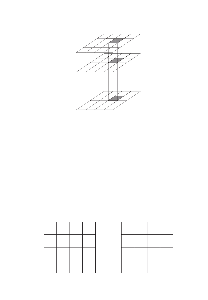
54
KEY CONCEPTS AND TECHNIQUES IN GIS
2
0
1
1
2
3
0
4
4
2
3
1
1
2
6
0
3
3
6
9
0
12
12
6
9
3
3
6
×
3
=
Figure 41
Multiplication of a raster layer by a scalar
are of the same size and orientation), and that the calculations themselves can often
be executed within the processor itself, which makes it extremely fast. So, although
a million cells may be processed, the result of a local operation is often instanta-
neous. Compare this to the complexity of overlay operations in the vector world (see
Chapter 6)!
Local map algebra functions can be arithmetic, trigonometric, exponential, loga-
rithmic, statistical or logical in nature. A trivial example would involve only one
input layer, where we multiply all cell values by a constant value, say ‘3’. As a result,
we could have an elevation layer, where the ratio of horizontal to vertical distances
is now exaggerated enough to visually discern terrain features (see Figure 41).
One notch up on the ladder of sophistication is the use of a multiplier layer (see
Figure 42). Say we have counties with different property tax rates. We could then
calculate not just purchase prices but long-term costs by multiplying the costs of
Local
Figure 40
Local function
Albrecht-3572-Ch-08.qxd 7/13/2007 4:16 PM Page 54

MAP ALGEBRA
55
each property by the tax rates. Observe what happens to the cells with no values;
NoData times something results in NoData.
8.3 Focal functions
Neighborhood or focal functions are the main reason for the success of map alge-
bra. Local functions, in a way, are nothing but fancy recoding operations, which
could indeed easily be performed in a proper database management system. Focal
functions, on the other hand, take into account all cells in a user-defined neighbor-
hood. Anybody who ever tried to calculate a cell value in a spreadsheet based on a
combination of surrounding cells knows that the query string very quickly becomes
really complicated. Again, the procedure is one cell at a time, except that for the
calculation of an output cell value, we now look at all cells surrounding the process-
ing location of all input layers (see Figure 43).
2
0
1
1
2
3
0
4
4
2
3
1
1
2
6
0
3
3
6
9
0
12
12
6
9
3
3
6
12
0
3
3
12
27
0
48
48
12
27
3
3
12
×
=
Figure 42
Multiplying one layer by another one
Focal
Figure 43
Focal function
Albrecht-3572-Ch-08.qxd 7/13/2007 4:16 PM Page 55

56
KEY CONCEPTS AND TECHNIQUES IN GIS
By default, the neighborhood is defined to be all eight cells touching the processing
cell, plus the processing cell in the middle. As an interesting aside, the first step of
a focal function uses only three neighboring cells because cell (1,1) sits in a corner
and has no more neighbors. Many GIS allow us to define different neighborhoods,
though. We may change the extent (size) of the neighborhood, its shape, or its ker-
nel (where in relationship to the neighborhood sits the operating cell?).
Just about any function type (arithmetic, trigonometric, exponential, logarithmic,
statistical or logical) that we encountered for local functions is also applicable for
focal functions. In addition, we have functions that compare cell values within a
neighborhood, rather than across multiple input layers. This way, we can determine
the average, minimum or maximum value within the neighborhood or calculate the
span (range) of values. One of the attractive features of map algebra is its naming
conventions. Identifiers such as FocalSum, FocalMean, LocalAND or ZonalMax are
more or less self-explanatory, yet this is exactly how all map algebra functions are
formed. Actual vendor implementations change a little bit in their semantics (e.g.
average versus mean) but stick to the principle.
Figure 44 describes a prominent focal function that is the basis for many image
processing operations. You are encouraged to work the example, or at least the first
row of cells in Figure 44. Remember to include the processing cell in all calcula-
tions. We will revisit neighborhood functions in Chapter 9, as the very notion of
terrain is a focal one.
2
0
1
1
2
3
0
4
4
2
2
3
3
1
1
2
1.8
1.3
1.5
1.5
2.2
2.0
1.8
1.8
2.2
2.0
2.2
2.3
2.0
2.2
2.2
2.5
=
Figure 44
Averaging neighborhood function
8.4 Zonal functions
Zonal functions are in effect a mixture of local and focal functions. Based on
Tobler’s First Law of Geography (see Chapter 10), cells of similar values can be
expected to lie next to each other. Hence everything that was said about focal func-
tions applies to zonal functions as well. On the other hand, more important than
spatial contiguity is the fact that all cells within a zone have the same value and they
are treated the same. Zonal functions therefore take on the character of recoding
functions that typified local functions.
Albrecht-3572-Ch-08.qxd 7/13/2007 4:16 PM Page 56

MAP ALGEBRA
57
The process is a bit more complicated than before. Again, zonal functions work
on a cell-by-cell basis. However, the zone now acts as a kind of variable neighbor-
hood definition (see Figure 45), and the zonal input layer as a lookup table. A zonal
function processes at least two input layers, one so-called zone layer, and one
or more value layers. The zones can be (and usually are) but do not have to be
contiguous.
Zonal
Figure 45
Zonal function
Figure 46 is an abstract example for a ZonalMax function. Again, as all map alge-
bra functions, it starts at cell (1,1), and looks what zonal number it contains. Then it
looks at all other cells with the same zonal number and creates a list of their values
from the second input layer. Upon determining the maximum value, it writes that
value to cell (1,1) in the output layer and proceeds to the next cell. If that next cell
has the same zonal number then the output value from the previous step is written to
cell (1,2). If the zonal number is different, then a new list of values belonging to all
cells of the new zone number is created and its maximum is written to cell (1,2). In
practice, the zonal number grids represent classified images or thematic maps, where
we run calculations on the value layer based on the cell’s membership to one class
or another.
8.5 Global functions
Global functions differ from the rest in that many of the arithmetic or statistical
operations do not make sense if applied globally (they would result in the same
value for all cells of the output grid). Instead, global functions determine the spatial
relationship between cells of interest – or in other words, the distance between cells.
Albrecht-3572-Ch-08.qxd 7/13/2007 4:16 PM Page 57

58
KEY CONCEPTS AND TECHNIQUES IN GIS
There are two types of global or distance function, Euclidean and weighted. The for-
mer is a straightforward geometric calculation, while the latter involves a second
input layer that encodes a cost or friction surface. With global functions, it is fairly
easy to implement the most complicated vector GIS operations: Thiessen polygons,
corridors and location–allocation.
8.6 Map algebra scripts
One of the most convincing arguments for map algebra was Tomlin’s use of map
algebra scripts, a concatenation of functions that represents a complete GIS analysis
workflow or even a dynamic model. While Tomlin just used simple sequences,
authors like Kirby and Pazner (1990), Wesseling and van Deursen (1995) and Pullar
(2003) developed temporal constructs that mimic classic programming languages
augmented by spatial expressions. A simple example is the following script, which
models the spread of a pollutant from a point source:
For
i = 1 to 100
plume = buffer(plume)* 1/
i
One of the interesting characteristics of most raster-based programs (particularly
image processing packages) is that the target file can be overwritten in a program-
ming loop. This saves disk space but of course prevents the analysis of intermediate
steps. Scripts are also the mechanism behind the raster-based terrain modeling oper-
ations discussed in Chapter 9.
2
2
1
1
2
3
3
1
2
3
1
1
2
2
1
2
3
4
5
6
7
8
1
2
3
4
5
5
5
5
5
5
8
8
5
7
8
7
8
5
8
8
5
5
=
Zone grid
Value grid
Figure 46
Value grids as spatial lookup tables
Albrecht-3572-Ch-08.qxd 7/13/2007 4:16 PM Page 58

All GIS functionality discussed so far assumed the world to be flat. This is, of
course, utterly unrealistic but GIS has succeeded in getting away with this deficiency
surprisingly well. Since 3-D representations are commonplace in modern CAD soft-
ware, the obvious question is why has GIS not followed suit? The answer lies in the
distinction between mere data representation that is common to CAD and vector
GIS, on the one hand, and the spatial reasoning capacity that is unique to GIS.
In general, we can distinguish between three different ways to represent the third
dimension (see Figure 47). One is the use of true three-dimensional coordinates to
construct what in CAD is called a wire frame model. The second uses the same
coordinates but constructs a mesh of triangles to drape a surface going through all
the points. Applied to relatively small areas but at high precision, this data structure
is often used in civil engineering applications. The last uses raster cells and records
for each cell an elevation value as the pertinent attribute. The image of the raster
surface in Figure 47 indicates a fourth representation, the use of contour lines. They
are a filter on the former, leaving only values at certain intervals, which are then
connected by a polyline. As we have seen earlier, the way we organize data directly
determines what kind of questions we can ask of the data. The wire frame model is
up to now the most limited of 3-D GIS models, serving mostly rendering functions
similar to those of architectural software packages.
9
Terrain Modeling
3-D wire frame
Raster surface
Snow depth
Tin
Figure 47
Three ways to represent the third dimension
Albrecht-3572-Ch-09.qxd 7/13/2007 5:09 PM Page 59
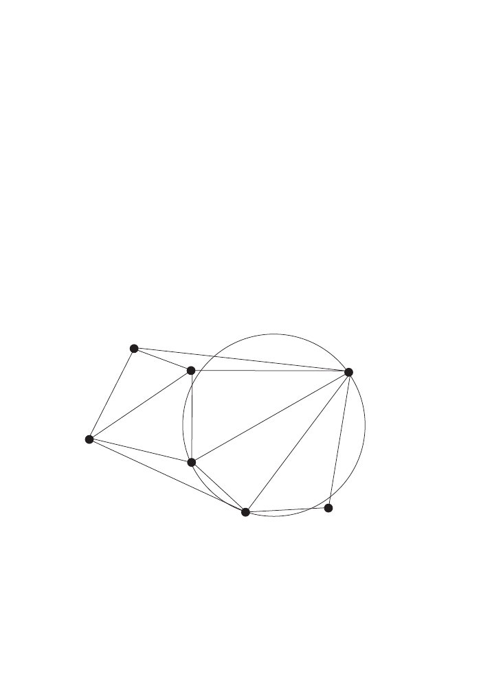
60
KEY CONCEPTS AND TECHNIQUES IN GIS
9.1 Triangulated irregular networks (TINs)
While the wire frame data at least in theory allows for a truly three-dimensional rep-
resentation (i.e., multiple objects intersecting with each other in all three dimen-
sions), triangulated irregular networks or TINs are used for surfaces only. This may
look like a limitation but it is not because none of the readily available off-the-shelf
GIS have extended their analytical capacities to the third dimension. TINs are func-
tionally a hybrid between the precise point representations typical for vector data
and the field view of raster data; as a matter of fact, we could interpret them as an
agglomeration of tiny fields, each represented by a triangular area. The triangles sat-
isfy the Delaunay criterion, which ensures that no node lies within the interior of any
of the circumcircles of the triangles (see Figure 48). This assures that the minimum
interior angle of all of the triangles is maximized and long, thin triangles are
avoided. In the process of calculating the best fitting triangles between all the points
that make up a given surface, the GIS determines and stores slope and aspect of
each. This is useful for two reasons. For one, this information is used in the render-
ing of 3-D surfaces and speeds up the process of displaying intricately shaded ter-
rain. Second, it makes it easy to calculate volumes of irregularly shaped bodies – a
task of particular pertinence in civil engineering.
G
F
E
D
C
A
B
Figure 48
Construction of a TIN
TINs and raster-based elevation models are often contrasted as incorporating the
classic difference between raster and vector GIS – the former being simple but either
imprecise or huge; the latter being complicated, precise and very efficient. In prac-
tice, the precision of TINs is a function of how precise the original measurement
was – which can be surprisingly poor in the third dimension. Also, most useful TINs
consist of millions of points, either because of how they were derived from raster
Albrecht-3572-Ch-09.qxd 7/13/2007 5:09 PM Page 60

TERRAIN MODELING
61
datasets, or because the surfaces used for civil engineering are so varied and have to
reflect many sharp edges that we would not encounter in natural settings. The main
difference then boils down to TINs being used (as the name implies) where we have
irregularly spaced measurements, and raster-based elevation models being regular.
9.2 Visibility analysis
Viewshed analysis was originally a classical raster GIS function, typically applied to
forest clear cuts in an attempt to determine which areas are visible from a road and
should hence be left to avoid the wrath of environmentalists (Bettinger and Sessions
2003) (see Figure 49).
Figure 49
Viewshed
When cellphone usage took off in the 1990s, providers looked for tools that would
help them to maximize coverage and minimize efforts for optimal placement of cell-
phone towers. The challenge for these companies was twofold. On the one hand they
had to provide nationwide coverage as fast as possible and digital elevation models
(see next section) are the obvious choice for that. On the other hand, the majority of
customers are located in cities with a very different and impeding topography, which
is better represented by TINs that are derived from high-resolution imagery.
Cellphone signals travel the same way as light does, and more important are
obstructed in a similar way. In a raster environment, we are hence looking at a
repeated zonal buffer operation. Due to the different data structure, the algorithms
for a TIN work very differently; they are based on the same computational geome-
try that film studios now use for rendering.
Albrecht-3572-Ch-09.qxd 7/13/2007 5:09 PM Page 61

62
KEY CONCEPTS AND TECHNIQUES IN GIS
9.3 Digital elevation and terrain models
Raster-based digital elevation models (DEMs) are by far the most common basis for
dealing with the third dimension. As a matter of fact, many people have difficulties
conceptualizing a raster attribute as anything but elevation. This is especially true for
digital elevation models that cover larger areas. There are two reasons for this. For
one, automated data capture for large areas tends to involve remote sensing methods
that result in raster datasets. As important, however, is the fact that map algebra
offers a plethora of analytical methods that require nothing but elevation and result
in an astounding array of derivatives.
In Chapter 8, we saw how focal or neighborhood operations are used to analyze
the combined spatial and attribute relationship between locations. The first set of
focal operations transforms a DEM to a digital terrain model or DTM. The differ-
ence between the two is that the latter stores, in addition to mere elevation, two
important derivatives – slope and aspect (see Figure 50). Slope is the ratio of eleva-
tion difference between the higher neighbors and the lower neighbors, and horizon-
tal distance between those neighbors. It is usually calculated based on the
8-neighborhood, which in turn defines the distance as twice the cell width in the
cardinal directions, and
√
2 times the former distance for the diagonals. Once we
know the slope at each cell location, it is another simple focal operation to compare
all neighbors and determine in what direction the surface slopes; this is called
aspect. Given that both operations are fairly simple, and that processing power of
modern computers is sufficient to calculate slope and aspect efficiently, DTMs are
decreasing in importance.
Aspect
Slope
36%
20
°
14
°
8.5
°
2.9
°
1.1
°
25%
15%
5%
0
45
90
135
180
225
270
315
2%
Figure 50
Derivation of slope and aspect
Albrecht-3572-Ch-09.qxd 7/13/2007 5:09 PM Page 62
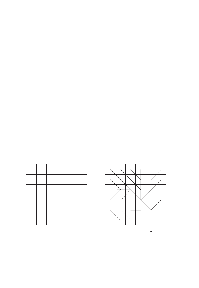
TERRAIN MODELING
63
9.4 Hydrological modeling
Slope and aspect are the cornerstones of hydrological modeling. The underlying
principle is fairly simple – and sometimes the application of out-of-the-box hydro-
logical GIS functions is a bit simplistic. The idea is that once we know slope and
aspect, we have a fairly good idea in what direction a drop of water would run off
once it hits the surface. Clearly, in reality this is applicable only in either barren
terrain or on totally saturated soils. On the other hand, all these complications can be
(and are) addressed by more complicated map algebra scripts that combine infiltra-
tion and runoff models.
To get back to the basic idea, once we know into which neighboring cell a drop of
water would flow, we can derive a flow direction map for the whole study area, which
in turn becomes the basis for a flow accumulation map (see Figure 51). Basically, what
happens here is that we look at each cell from the point of view of how many cells it
receives from, and into which cell it passes its accumulated flow. We are virtually drain-
ing the terrain, and as a result see where streams would flow (Wilson & Gallant 2000).
As mentioned above, this simple perspective works best in ‘well-behaving’ terrain,
where there is a discernable slope and the land cover is not too variable. Under those
conditions the resulting runoff calculation is surprisingly accurate; and with ever-
increasing precision of DEM data, a range of national and international organizations is
currently developing sophisticated hydrological models. The work at the University of
Texas’ Center for Research in Water Resources is fairly representative for these endeav-
ors; their efforts to provide access to all their models and data via their website at
http://www.crwr.utexas.edu/ is exemplary.
0
0
0
0
0
0
0
1
1
2
2
0
0
3
7
5
4
0
0
0
0
20
0
1
0
0
0
1
24
0
0
2
4
7
35
1
0
0
0
0
0
0
0
1
1
2
2
0
0
3
7
5
4
0
0
0
0
20
0
1
0
0
0
1
24
0
0
2
4
7
35
1
Figure 51
Flow accumulation map
Two aspects of hydrological modeling deserve extra mention. As can be seen
from these four sections, all we needed in the beginning was a DEM. Each of the
maps was a direct result of applying one operation or script to its predecessor. It is
therefore fairly straightforward to write a rather longish script that creates all the
Albrecht-3572-Ch-09.qxd 7/13/2007 5:09 PM Page 63

64
KEY CONCEPTS AND TECHNIQUES IN GIS
intermediate files and derives a flood forecast model in one go – a prime example
for the power of map algebra. Second, impressive as all of this is, it provides only a
hint at all the models that can be developed and linked with each other. For exam-
ple, based on a comparison of satellite images, we can develop models of urban
sprawl and impervious surfaces. These can then be linked with the runoff model
above to develop true simulation models, possibly linked with real-time readings of
precipitation.
All of the above are true terrain modeling applications. The methods discussed in
this chapter are, however, just as applicable to artificial surfaces, where the third
dimension represents an attribute value such as property value or air pollution. These
kinds of surfaces are typically interpolated from sparse measurements. The follow-
ing chapter will cover spatial interpolation techniques and more.
Albrecht-3572-Ch-09.qxd 7/13/2007 5:09 PM Page 64

This chapter consists of two distinct parts because the phrase ‘spatial statistics’ has
two rather different meanings, depending where one comes from. The first comes
from a geophysics background and is also known as geo-statistics. The second has
its roots in analytical cartography and is known as spatial analysis.
10.1 Geo-statistics
Typically, stochastic methods are applied when we have lots of data but not a really
good idea of what drives the data. Deterministic models, on the other hand, are used
when the data is sparse but we are confident that our understanding of the phenom-
enon, say based on a long history of similar observations, is good. The following set
of methods cover both approaches, although the underlying commonality is a
scarcity of data. All spatial interpolation techniques discussed here aim at creating
surfaces from point data. It is important to recognize that most applications are not
in terrain modeling but that the surfaces are intended to allow estimates of any kind
of continuous variable, such as pollution, crime or mineral resources.
All model-based interpolation methods assume Tobler’s (1970) First Law of
Geography, which basically means that everything is related to everything else, but
things that are closer in space (i.e., neighbors) are also closer with respect to their
attribute values. There are many interpolation methods and we use some descriptors
to categorize them by the number of input values (local versus global methods) and
the characteristics of the resulting surface. If the surface goes through the values of
known locations, then we label a method as exact. Otherwise we refer to it as a
smooth interpolator, because the resulting surface avoids ruggedness around meas-
ured locations. The most common of these methods are inverse distance weighting
(IDW), polynomials and splines.
10.1.1 Inverse distance weighting
IDW is the most direct implementation of Tobler’s First Law (see Figure 52). Given
known values at some locations, we try to determine the most probable value at a
location for which we don’t have a measurement.
The calculation is made up of known values of neighboring locations, which are
weighted according to their distance from the one location for which we want to
determine a value. This calculation is repeated for as many points as we care about.
If the surface to be created is based on a TIN data structure, then we probably only
double or triple the number of original points. If the surface is a raster dataset, then
10
Spatial Statistics
Albrecht-3572-Ch-10.qxd 7/13/2007 5:09 PM Page 65

66
KEY CONCEPTS AND TECHNIQUES IN GIS
the calculation is repeated for every cell for which we don’t have a measurement.
The implementation of IDW differs among software packages, but most of them
allow specification of the number and or distance of known values to be included,
and in order to function properly they must allow for the user to specify the rate at
which a location’s weight decreases over distance. The differences lie in how sophis-
ticated that distance–decay function can be. Because IDW calculates new values
only for points for which no measurements exist, it does not touch the values of
known locations and hence is an exact interpolator.
10.1.2 Global and local polynomials
Most readers will remember polynomials from their high school geometry classes.
These are equations that we use to fit a line or curve through a number of known
points. We encountered them in their simplest form in the calculation of slope, usu-
ally described in the form y = a + bx. Here we fit a straight line between two points,
which works perfectly well in a raster GIS, where the distance from one elevation
value to the next is minimal.
If the distance between the measured point locations is large, however, then a straight
line is unlikely to adequately represent the surface; it would also be highly unusual for
all the measured points to line up along a straight line (see Figure 53). Polynomials of
second or higher degree (the number of plus or minus signs in the equation determines
the degree of a polynomial) represent the actual surface much better.
Increasingly higher degrees have two disadvantages. First, the math to solve higher
degree polynomials is quite complicated (remember your geometry class?). Second,
even more importantly, a very sophisticated equation is likely to be an overfit. An over-
fit occurs when the equation is made to fit one particular set of input points but gets
thrown off when that set changes or even when just one other point is added. In prac-
tice, polynomials of second or third degree have proven to strike the best balance.
We distinguish between so-called local and global polynomials, depending on
whether we attempt to derive a surface for all our data or for only parts of it. By their
very nature, local polynomials are more accurate within their local realm. It depends
on our knowledge of what the data is supposed to represent, whether a single global
P
= 0
P
= 1
P
= 2
20
15
10
5
Relative Weight
Distance
0
1.0
0.8
0.6
0.4
0.2
0.0
Figure 52
Inverse distance weighting
Albrecht-3572-Ch-10.qxd 7/13/2007 5:09 PM Page 66

SPATIAL STATISTICS
67
polynomial is sufficient, or whether we need to subdivide the study area into regions
(see Figure 54). Especially, lower degree polynomials are smooth interpolators – the
resulting surface tends to miss measured values.
10.1.3 Splines
Splines are a common function in CAD packages, where the goal is to create smooth
surfaces that minimize turbulence. The word originally described a long piece of
wood that is bent by attaching weights along its length, pulling it into a desired shape
(e.g. the outline of a violin or a ship’s hull – see Figure 55).
Starting in the 1940s, mathematicians used the idea of weights pulling orthogo-
nally to a line to develop rather complicated sets of local polynomials. They refer to
splines as radial basis functions. The calculation of splines is computing intensive;
the results definitely look pretty but may not be a good characterization of a natural
landscape. Similar to IDW, the input points remain intact (see Figure 56) – which
means that splines, in spite of their smooth appearance, actually are exact interpola-
tors (see Figure 57).
First order
Second order
Figure 53
Polynomials of first and second order
Global
(all points are considered at once)
Local
(only a few points at a time considered)
Figure 54
Local and global polynomials
Albrecht-3572-Ch-10.qxd 7/13/2007 5:09 PM Page 67
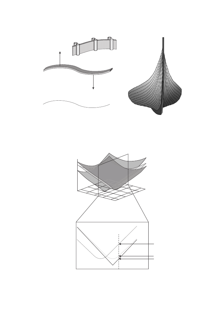
68
KEY CONCEPTS AND TECHNIQUES IN GIS
Bending of a Plank
Abstraction
Final Product
Figure 55
Historical use of splines
1
10
10
8
8
6
6
6
X
8
10
6
X
Y
4
4
4
4
2
2
2
0
2
234
Z
Z
567
Φ
3
Φ
2
Φ
3
Figure 56
Application of splines to surfaces
Albrecht-3572-Ch-10.qxd 7/13/2007 5:09 PM Page 68

SPATIAL STATISTICS
69
10.1.4 Kriging
All of the above interpolation methods use a model of what the analyst believes is
the best representation of the interpolated surface. Kriging does this too; however,
it uses statistics to develop the model. Originally developed for applications in the
mining industry, it is now widely used in epidemiology, the environmental sciences,
and of course geophysics. The term ‘kriging’ now signifies a whole family of meth-
ods, which to explain would go way beyond the scope of this book. The following
is therefore only a general description of what underlies all kriging methods.
Kriging adopts the simple polynomial view of the world but concentrates on the
tail end of the equation – called error – that describes what is not captured by the
equation proper. In
y
=
a
+ bx + cx
2
+ e
for instance, we have a second-degree polynomial with an error term e, which basi-
cally is a vessel for all discrepancies between the model result and the observed out-
come (remember, polynomials are smooth or inexact interpolators). Using the First
Law of Geography, it is now fair to assume that all the errors are spatially autocorre-
lated – that is, they increase the further we get away from a measured point. Kriging
uses a brute force method of computing the relationships between all measured points
and then runs statistics over the resulting table to determine which points have how
much influence on what other points. This information is then fed back into the sur-
face equation, which ideally is then error-free, making kriging an exact interpolator.
In practice there are a number of complications, each of which is addressed by a
particular kind of kriging method. Especially the more sophisticated forms of krig-
ing are extremely computing intensive; the results are no great shake if the number
of original measurements is too small and the calculations run out of bounds if we
have a rich input dataset. For the right number of points, and if the computing power
is available, kriging delivers very robust results.
Exact:
never exceeding
given values
Exact:
possibly exaggerating
Figure 57
Exact and inexact interpolators
Albrecht-3572-Ch-10.qxd 7/13/2007 5:09 PM Page 69

70
KEY CONCEPTS AND TECHNIQUES IN GIS
10.2 Spatial analysis
Spatial analysis comprises of a whole bag of different methods dealing with the
quantitative analysis of spatial data. It ranges from simple geometric descriptors to
highly sophisticated spatial interaction models. In a narrow sense, spatial analysis is
the decidedly pre-GIS set of methods developed by geographers during the quanti-
tative revolution of the 1960s, who in turn borrowed from analytical cartographers.
Their goal was to describe geographic distributions, identify spatial patterns, and
analyze geographic relationships and processes – all without GIS and often enough
even without anything close to a computer.
10.2.1 Geometric descriptors
This is the application of descriptive statistics to spatial data. While we may some-
times borrow directly from traditional statistics, more often than not spatial also
means special. In other words, we will have to come up with procedures that capture
the spirit of what the traditional methods try to accomplish but adjust their imple-
mentation to the multi-dimensionality of spatial data, and possibly more important
to the fact that we cannot assume spatial samples to be independent of each other.
We referred to the phenomenon of spatial autocorrelation above but did not
expand on what a nuisance it poses for the statistical analysis of spatial data.
Traditional statistics is based on the fact that samples are taken independently of
each other and most methods assume a normal distribution. Both of these assump-
tions do not hold with geographic data – if they did, then there would be no basis for
the discipline of geography. If a distribution is random then it is decidedly non-
geographic, and Tobler’s First Law of Geography would not hold.
The most basic descriptors in traditional statistics are mean, mode and standard
deviation. Of these, the mean is relatively easy to translate into a spatial context; we
just have to make sure that we calculate the average along as many dimensions
(typically 1 to 3 for transects, areas or volumes) as we need. Figure 58 gives an
example of a geometric mean.
The geometric median is a bit different from its traditional counterpart.
Calculating the median values along x, y and possibly z to then mark the median
location does not capture what we usually strive for in the calculation of a median.
In traditional statistics, the median marks the point that is as far away from one end
of the distribution as from the other. Translated into the spatial realm, this means
that we are looking for a location that does the same not just within a dimension but
also across. As it turns out, this is a really useful measure because it describes the
location that minimizes the combined distances from that central point to all other
locations. Unfortunately, there is no simple equation for that – the point can be found
only through iterative optimization. Figure 59 illustrates the difference between a
spatial mean and a spatial median.
A simple measure of central tendency is often too crude to adequately describe a
geographic distribution. Analogue to the standard deviation in traditional statistics,
Albrecht-3572-Ch-10.qxd 7/13/2007 5:09 PM Page 70

SPATIAL STATISTICS
71
we can employ standard distance as the circle around the mean, which captures a
significant number of neighbors. The smaller the circle the more compact is the phe-
nomenon; a wide circle tells us that the spatial mean is not very representative.
However, by just calculating the standard distance, we throw away a lot of additional
information. If we separate the standard distance into its x and y components, we get
a standard deviational eclipse (see Figure 60) that tells us about the orientation or
direction of the phenomenon and hence gives us additional clues as to what causes
or at least influences it. This even applies to linear features, as a multitude of paths
distributed over a larger surface (e.g. hurricanes or a river network) provides valu-
able clues as to what forces a change in direction.
The field of spatial pattern descriptors was expanded by landscape ecologists in
the 1980s, who developed a myriad of measures to describe shapes and geometric
relationships between features. Shape measures (see Figure 61) try to come up with
characteristic numbers such as the ratio of edge length to area size, the degree of
roundness (with a circle being perfectly round), or a figure for a feature’s fractal
dimension. While we will discuss more advanced spatial relationships in the next
section, it is worthwhile to mention that a number of landscape ecological measures
calculate average, min and max distance between features in general and on a fea-
ture class by feature class basis.
22
20
18
16
14
12
10
8
6
4
2
2
4
6
8
10
12
14
16
18
20
22
Figure 58
Geometric mean
Albrecht-3572-Ch-10.qxd 7/13/2007 5:09 PM Page 71

72
KEY CONCEPTS AND TECHNIQUES IN GIS
10.2.2 Spatial patterns
All of the above are global descriptors; they work well if the phenomenon we are
studying is evenly distributed across the study area. But those are not the interesting
geographic research questions. If we want to pursue locational variation then we
need descriptors of local change. Although it sounds like an oxymoron, we have both
global and local descriptors or local change.
Similar to the way we measure confidence in traditional statistics, we use the dif-
ference between observed distributions and expected (using the null hypothesis of
randomness) to determine the degree of ‘geography-drivenness’. Unfortunately, this
is a bit more difficult than in traditional statistics because the numbers (and hence
our confidence) change depending on how we configure size and origin of the search
window within which we compare the two distributions.
One of the most often used spatial analytical methods is a nearest-neighbor analy-
sis. Here we measure for each feature (zone in the raster world) the distance to its
nearest neighbor and then calculate the average, min or max distance between neigh-
bors of the same class or neighbors of two classes that we want to juxtapose with
each other. Again, we can use a comparison between observed versus expected
nearest-neighbor distance to in this case describe a particular distribution as clus-
tered, random or dispersed. When we do this repeatedly with ever-changing search
22
20
18
16
14
12
10
8
6
4
2
2
4
6
8
10
12
14
16
18
20
22
Figure 59
Geometric mean and geometric median
Albrecht-3572-Ch-10.qxd 7/13/2007 5:09 PM Page 72

SPATIAL STATISTICS
73
window size, we find the scale at which a given spatial pattern is particularly promi-
nent, which in turn helps us to identify the process that is driving the spatial pattern.
So far, we have assumed that all features either belonged to one and the same class
or to a limited number of classes, for which we then describe the respective spatial
22
20
18
16
14
12
10
8
6
4
2
2
4
6
8
10
12
14
16
18
20
22
Figure 60
Standard deviational ellipse
High Value
Low Value
Area
Edge
Shape
Diversity
Core
Area
Nearest
Neighbor
Patch
Density
Figure 61
Shape measures
Albrecht-3572-Ch-10.qxd 7/13/2007 5:09 PM Page 73
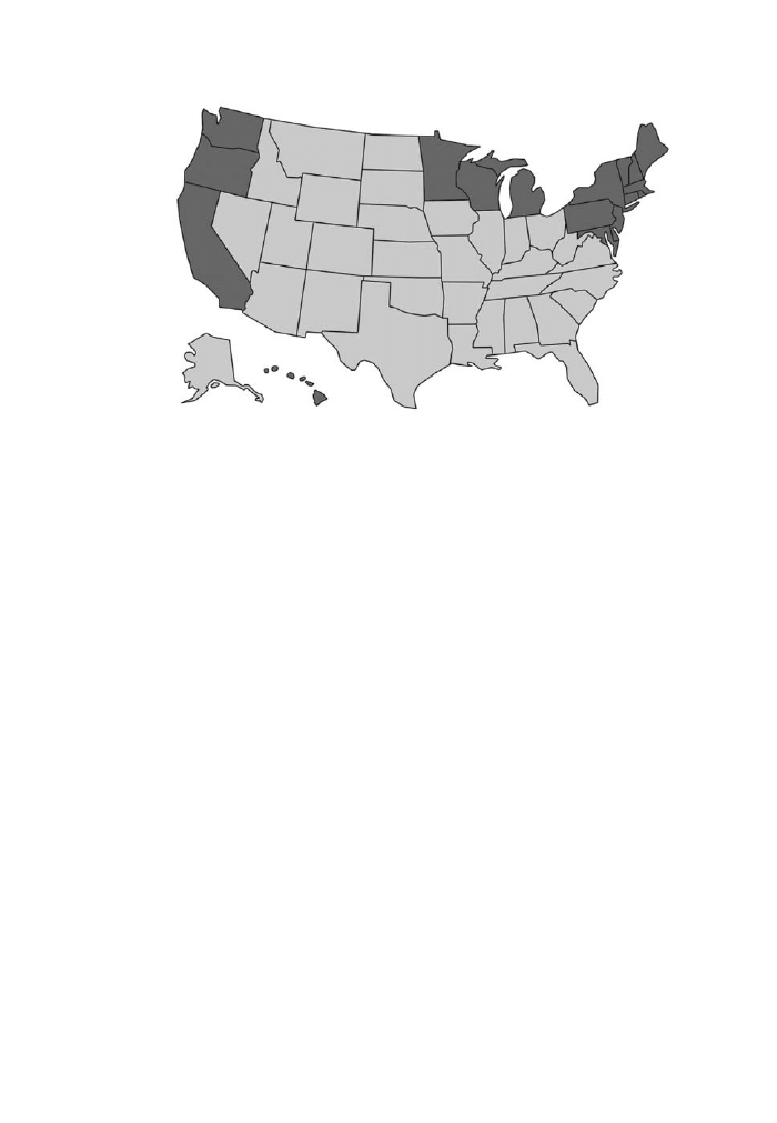
74
KEY CONCEPTS AND TECHNIQUES IN GIS
relationship. Alternatively, we could look at the attribute values of neighboring fea-
tures and try to determine how similar or dissimilar they are. Common measures for
the similarity of neighboring features are Geary’s contiguity ratio c and Moran’s I,
and more recently the general G-statistic, which measures the degree of concentra-
tion of high versus low values. For categorical values, finally, we can use a so-called
joint-count statistic, which compares the observed combination of neighboring val-
ues with a random combination. Figure 62 is a joint-count statistic of blue versus red
states in the 2004 presidential elections in the United States.
All of the above is commonly applied to Euclidean distances but all of these
measures work just as well on cost distances. And last but not least, the pattern ana-
lyzers can be applied to regional subsets, which often is more telling than a global
measure.
10.2.3 The modifiable area unit problem (MAUP)
As mentioned at the beginning of the previous section, there are both global and
local pattern detectors. The problem with the local ones, although they would be
much more specific, is that it is hard to tell how to draw the boundaries. And as if
this is not enough, more often than not the local boundaries for our data are
predetermined. When we want to work with census data, for instance, we do not
have control over how the data is collected or aggregated, and numerous studies
have proven that, by drawing different boundaries, the results of a spatial analysis
could be completely reversed. Without access to non-aggregated data, this is a severe
limitation of spatial analysis, similar though not the same as the ecological fallacy
problem in traditional statistics.
Figure 62
Joint count statistic
Albrecht-3572-Ch-10.qxd 7/13/2007 5:09 PM Page 74

SPATIAL STATISTICS
75
10.2.4 Geographic relationships
Another major contributor to spatial analysis techniques is the discipline of regional
science, somewhat of a hybrid between economic geography and spatial economet-
rics. Some of the network-based location–allocation models come out of that realm,
but what interests us here is the use of systems of regression equations to represent
these relationships between geographic features. The polynomials that we encoun-
tered in geostatistics can be used the other way around – not to calculate missing val-
ues but to determine the underlying forcing functions that result in the observed
values. Although there are examples for global regression analysis, the local (also
known as geographically weighted) regression is of particular interest.
Many of these calculations are computationally very expensive, especially
because an unbiased analysis requires the repeated run of many scenarios, where
parameters are altered one at a time (Monte Carlo analysis). The frustration with this
Pandora box of spatial analysis problems led to the development of geo-computation
as a field, where the latest information science methods are applied to solving
uncomfortably large spatial analysis problems. We look at these in the next chapter.
Albrecht-3572-Ch-10.qxd 7/13/2007 5:09 PM Page 75

Albrecht-3572-Ch-10.qxd 7/13/2007 5:09 PM Page 76

Geocomputation is a set of computational methods that has been customized to
address the special characteristics of spatial data. Given that definition, GIS would
be a geocomputational method but it is decidedly not. The term was invented by
geographer Stan Openshaw and became institutionalized with the first Geo-
Computation conference in 1996. The term ‘computational’ has come to replace what
used to be known as artificial intelligence techniques: from genetic algorithms, neu-
ral networks, and fuzzy reasoning to cellular automata, agent-based modeling, and
highly parallelized processing. The common ground behind all of these is that if we
throw lots of processing power and the latest advances in information science at
large spatial datasets, then we have a good shot at deriving new insights.
A look at the proceedings of the GeoComputation conference series (www.
geocomputation.org) conveys the wide range of topics, far more than could be
covered in this chapter. We will concentrate here on five areas of research that have
matured more than others: fuzzy reasoning, neural networks, genetic algorithms,
cellular automata and agent-based modeling systems.
11.1 Fuzzy reasoning
As mentioned above, geocomputational techniques are borrowed from information
science and then applied to spatial data. Lofti Zadeh (1965) formalized a set of rules
to work with multi-valued logic, which allows us to capture the multi-valuedness of
our thinking. Rather than categorizing everything as yes/no, black/white, zero/one
etc., as we did when we introduced Boolean logic in Chapter 6, fuzzy logic extends
the hard values zero and one to everything in between. An attribute can now be a
little bit of green and a little more of blue rather than either green or blue. And
applied to geographic phenomena, Florida can be 10% tropical, 80% subtropical,
and another 10% moderate in climate.
The best everyday illustration of how fuzziness works is a shower knob that this
author found in the bathroom of a New Zealand colleague (see Figure 63). People
tend to have different opinions about what is warm water. By having the marking for
cold water become ever thinner as the marking for warm water increases in width,
the definition covers a wide range of beliefs with the majority somewhere in the
middle at around 45°centigrade.
11
Geocomputation
Albrecht-3572-Ch-11.qxd 7/13/2007 4:18 PM Page 77

Formally, we describe fuzziness as a set of values ranging from 0 to 1. The grade
to which an individual observation z is a member of the set is determined by a mem-
bership function, where membership values close to 1 represent observations close
to the core concept. The value of the membership function reflects a kind of degree
that is not based on probability but on admitted possibility. This concept of fuzziness
allows us to work with imprecision, describing classes that for various reasons do
not have sharply defined boundaries (Burrough and Frank 1996). The use of fuzzy
sets is appropriate, whenever one has to deal with ambiguous, vague and ambivalent
issues in models of empirical phenomena, and even supports working with qualita-
tive data.
Data in fuzzy sets can be manipulated using basic operations that are similar to
those found in Boolean logic – union (OR), intersection (AND) and negation (NOT).
These operations are employed on both the spatial and the attributive aspects of an
observation. The union operation (OR) combines fuzzy sets by selecting the maxi-
mum value of the membership function. The intersection operation (AND) requires
the selection of the minimum membership value of the fuzzy sets in question. These
operations perform the computation of a new membership value, which is called the
joint membership function value.
The beauty of fuzzy logic applications in GIS is that it (a) overcomes the sim-
plistic black/white perspective that traditional GIS forces us to adopt, and (b) it – at
least in theory – allows us to work with qualitative notions of space. The Conference
78
KEY CONCEPTS AND TECHNIQUES IN GIS
Hot
Warm
Cold
Figure 63
Shower tab illustrating fuzzy notions of water temperature
Albrecht-3572-Ch-11.qxd 7/13/2007 4:18 PM Page 78
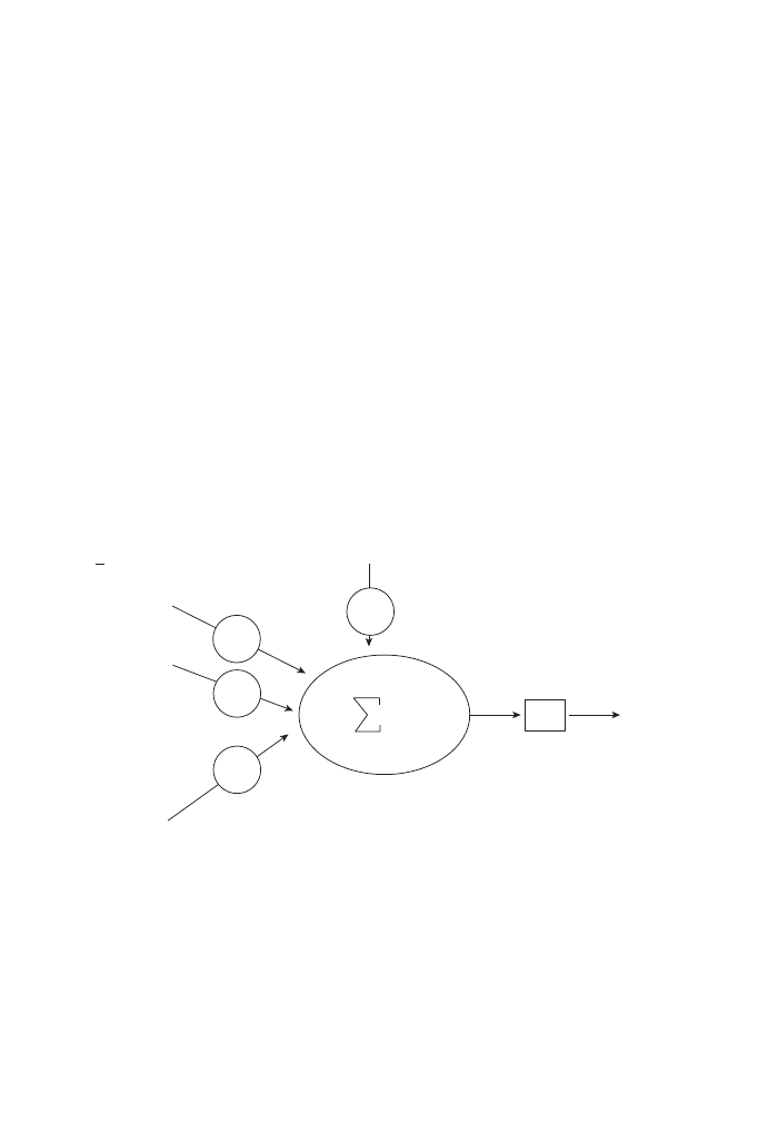
on Spatial Information Theory (COSIT) series is to a large degree devoted to the
development of methods of qualitative spatial reasoning; unfortunately not much of
the work presented there (1993–2005) has made it into readily available software.
11.2 Neural networks
With the advent of large spatial databases, sometimes consisting of terabytes of data,
traditional methods of statistics such as those described in the previous chapter
become untenable. The first group of GIScientists to encounter that problem was
remote sensing specialists, and so it is no surprise that they were the first to ‘dis-
cover’ neural networks as a possible solution. Neural networks grew out of research
in artificial intelligence, where one line of research attempts to reproduce intelli-
gence by building systems with an architecture that is similar to the human brain
(Hebb 1949). Using a very large number of extremely simple processing units (each
performing a weighted sum of its inputs, and then firing a binary signal if the total
input exceeds a certain level) the brain manages to perform extremely complex tasks
(see Figure 64).
GEOCOMPUTATION
79
Feature vector
Weights
(parameters)
Non–linear
Non–decreasing
Activation function
Threshold effect described as
an additional constant input:
X
0
= −1 (threshold)
X
0
= +1 (bias)
X
= (X
1
,X
2
,...X
n
)
t
X
0
= 1
X
1
X
2
X
n
W
1
W
2
W
3
W
0
v
y
n
i
= 0
W
i
X
i
ϕ(v)
Figure 64
Schematics of a single neuron, the building block of an artificial neural
network
Using the software (sometimes, though rarely, hardware) equivalent of the kind of
neural network that makes up the brain, artificial neural networks accomplish tasks
that were previously thought impossible for a computer. Examples include adaptive
learning, self-organization, error tolerance, real-time operation and parallel process-
ing. As data is given to a neural network, it (re-)organizes its structure to reflect the
Albrecht-3572-Ch-11.qxd 7/13/2007 4:18 PM Page 79

properties of the given data. In most neural network models, the term ‘self-organization’
refers to the determination of the connection strengths between data objects, the so-
called neurons. Several distinct neural network models can be distinguished both
from their internal architecture and from the learning algorithms that they use, but it
would be beyond the scope of this book to go into detail here.
An important aspect of neural networks is whether or not they need guidance in
learning. Based on the way they learn, all artificial neural networks can be divided
into two learning types – supervised and unsupervised (analogous to the same idea
in image classification used by remote sensers). In supervised learning, a desired
output result for each input vector is required when the network is trained. It uses the
target result to guide the formation of the neural parameters. In unsupervised learn-
ing, the training of the network is entirely data-driven and no target results for the
input data vectors are provided. A neural network of the unsupervised learning type,
such as Kohonen’s (1982) self-organizing map, can be used for clustering the input
data.
This alludes to the fact that the outcome of the application of neural networks is
nothing really new. All this wizardry results in pretty much the same regression
equations that we encountered in the previous chapter. There are two main differ-
ences. First, given the data volume, we could not have arrived at these results, which
is the positive aspect. On the downside, the results are data and do not give us any
insight into what is actually happening. From a scientific perspective, statistics is
supposed to help us understand how things work. Neural networks, however, act like
a black box – there is no algorithm (and no explanatory structure) that would help
us to understand the phenomenon we are studying.
11.3 Genetic algorithms
There is nothing inherently spatial in genetic or evolutionary programming, so the
reader might wonder why they became a popular geocomputational tool. Invented
by Holland (1975), they are the dynamic equivalent of neural networks. While the
latter are used when we have a large amount of data, genetic algorithms are used
when we have a large number of possible solutions. A nice spatial example is the
traveling salesman problem, where the task is to find the optimal sequence of cus-
tomers in a sequential path. The problem cannot be solved for more than a handful
of points because of the combinatorial explosion of options. This is, by the way, the
reason why computers have not yet been able to beat a good player of the Japanese
game of ‘Go’, another inherently spatial application. Genetic algorithms cannot
claim to find the absolute best solution, but they are very good at finding better solu-
tions than anyone or anything else.
I alluded to the use of genetic algorithms at the end of Chapter 7 (Location–
Allocation), when we found that the model becomes intractably complicated. When
we have a large number of origins and destinations, with multiple cases of each other
influencing weights, then the equations not only become long and complicated, but
80
KEY CONCEPTS AND TECHNIQUES IN GIS
Albrecht-3572-Ch-11.qxd 7/13/2007 4:18 PM Page 80

the possible solution space of varying parameters becomes as large as in our traveling
salesman problem, depicted in Figure 65. Who would venture a guess, which part of
the equation should be tweaked to improve the result?
GEOCOMPUTATION
81
Figure 65
Genetic algorithms are mainly applied when the model becomes too
complicated to be solved deterministically
Evolutionary programming starts by generating a population of purely random
expressions – that is, random model equations. These are evaluated in terms of a
fitness function. The best expressions are reused and sent to compete with a new
generation of crossovers and slightly mutated versions of previously successful
expressions. This process is repeated until no improvement is achieved. The terms
‘crossover’ and ‘mutation’ are borrowed from their biological analogues and func-
tion exactly the same way (see Figure 66). A crossover is a mixing of previously
successful strategies, while a mutation is a slight alteration. Together with the best
members of a previous generation, these new entities have to prove themselves. If
they succeed (i.e., fare better in the evaluation of fitness for a particular goal), then
they are allowed to stay for the next round.
Evolutionary techniques have not yet made it into commercially available GIS
packages, but public domain versions of linkages are available. The interested reader
may want to search www.sourceforge.net for a combination of the terms genetic and
GIS.
11.4 Cellular automata
CA are a modeling framework for spatially continuous phenomena (Langton 1986),
such as landscape processes or urban sprawl (Haff 2001; Box 2002; Silva and Clarke
2002). They are simple models used to represent the diffusion of things such as matter,
information or energy, over a spatial structure. In its most simple form, a CA is
Albrecht-3572-Ch-11.qxd 7/13/2007 4:18 PM Page 81
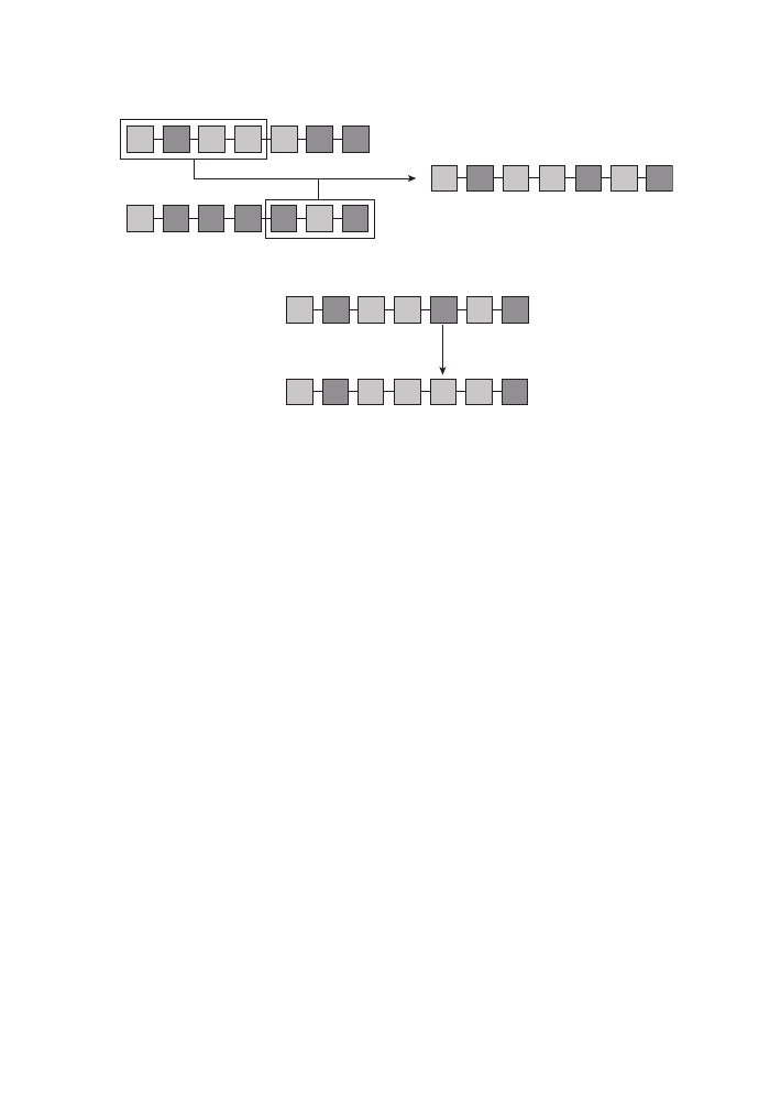
composed of a uniformly tessellated surface (typically a grid) whose cells may exist in
a finite number of discrete states (see O’Sullivan 2001 for extensions). As such, CA can
be considered a dynamic extension to raster GIS (Bian 2000). Each cell has an identi-
cally sized neighborhood consisting of nearby cells and a rule set defining how each cell
changes based on the state of its neighborhood. These changes can be a function of
either relative or absolute models of time, absolute time being where the scheduled tick
of the model clock defines the change, and relative time expressed as a cascading
process of event-based changes from one cell to the next. With these component parts,
the model is initiated and run where each cell in the CA checks its neighborhood and
changes its state based on the rules defining its behavior.
Despite the simplicity of construction, the dynamics of a CA model can produce
complex results. For example, O’Sullivan measures change as the record of the time-
series evolution of a measure of spatial pattern (2001).
However, CA are limited when it comes to modeling dynamic spatial phenomena.
The most important limitation is that the structure of the tessellation is typically
static, although there has been some promising experimentation with mutable CA in
urban modeling (Semboloni 2000), and the use of self-modifying rules to capture
nonlinear behavior (Silva and Clarke 2002). Yet there remains little scope for feed-
back and consequent self-organization of the cellular structure.
11.5 Agent-based modeling systems
Agent-based modeling (ABM), synonymous with individual-based modeling in
ecology (Bian 2000), is a simulation methodology focused on mobile individuals
and their interaction. It is based on the development of multi-agent systems (MAS),
82
KEY CONCEPTS AND TECHNIQUES IN GIS
Parent 1
Parent 2
Offspring
Before mutation
After mutation
1
0
1
1
1
0
0
1
0
0
0
0
1
0
1
0
1
1
0
1
0
1
0
1
1
1
1
0
1
0
1
1
0
1
0
Figure 66
Principles of genetic algorithms
Albrecht-3572-Ch-11.qxd 7/13/2007 4:18 PM Page 82

which were created in the field of distributed artificial intelligence (Gilbert and
Terna 2000).
‘Agent’ is a generic term used for any constituent entity whose behavior we wish
to model, and for its representation within the model. Agent-based models offer the
ability to capture the dynamic interactions of individuals and the context in which
they occur. Agent-based models enable the creation of ‘artificial societies’ which can
be viewed as laboratories in which to conduct experiments (Epstein and Axtell
1996). Agents are defined, placed in an environment and given a set of bounded
rules of behavior. The goal is to observe how interactions among individuals
produce the collective behaviors that are being studied.
An agent-based simulation implemented in the framework of a computational
laboratory offers the following advantages (Epstein and Axtell 1996; Gilbert and
Terna 2000). First, agent-based models allow heterogeneity among individuals that
more closely approximates the variety found in life. Second, the agents and the land-
scape can be held constant or systematically varied in order to provide a level of con-
trol impossible to attain using traditional social science methods. Third, the
combination of heterogeneous agents and control enables the researcher to conduct
a variety of experiments, using different conditions or applying various prevention
scenarios and then evaluating outcomes for minimal cost compared to experiments
in the real world. Using simulations allows us to repeat experiments under controlled
conditions and to compress spatio-temporal scales, so we are no longer limited to
observing just a few outcomes that happen to be presented by the real world. In addi-
tion, we are able to explore, evaluate and refine alternative scenarios and plans for
remediation safely and at reasonable costs and risks.
The observables or attributes of an agent (including spatial location) are meas-
urable characteristics of the agent that change over time (Parunak et al. 1998).
These observables describe the state of the system at any one time and are the pri-
mary output of an ABM. ABMs develop histories of system states, where, as with
temporal extensions to GIS, change is handled by storing the system state at each
time or by storing vectors of events for each agent; that is, an agent logs each new
state it enters. The focus of ABM is to understand the emergent outcome of each
model, where emergent ‘denotes the stable macroscopic patterns arising from
the local interactions of agents’ (Epstein and Axtell 1996, p. 35). In terms of
spatial ABMs, this is the spatial pattern of observables (e.g. Parker and Meretsky
2004).
The primary distinction between CA and ABM is the conceptual primitive used to
represent phenomena. In CA, this primitive is a static cell or pixel, a collection of
which composes a layer of cells. Its dynamics involve each cell transferring infor-
mation to its neighboring cells. An ABM, in contrast, is composed of distinguishable
objects, the same geometric primitives of point, line or polygon data models found
in GIS. Agent-based modeling enables the dynamic, situation-based decisions of
individuals to drive emerging macro-level patterns of the phenomenon under study
and is indispensable to the modeling of individual-level decision-making.
Furthermore, an agent has the added advantage of being mobile.
GEOCOMPUTATION
83
Albrecht-3572-Ch-11.qxd 7/13/2007 4:18 PM Page 83

There has been interest in intelligent software agents in GIScience in a variety
of contexts. In particular, agents have been employed in geographic simulation
modeling of a variety of phenomena, including simulation of land-use/cover change
(Manson 2002; Parker et al. 2003), wayfinding (Raubal 2001) and social simulations
(Gilbert and Doran 1994; Epstein and Axtell 1996; Gilbert and Troitzsch 1999;
Conte et al. 2001). Only limited integration of GIS and agent-based models to
simulate social phenomena has been achieved (Gimblett 2002). Agent-based simu-
lation models are particularly promising for urban applications (Batty 2001;
Benenson et al. 2002; Deadman and Gimblett 1994; Dean et al. 2000; Westervelt
and Hopkins 1999).
84
KEY CONCEPTS AND TECHNIQUES IN GIS
Albrecht-3572-Ch-11.qxd 7/13/2007 4:18 PM Page 84

Many of the geocomputational techniques discussed in the Chapter 11 go beyond the
scope of commercial GIS. That is partly because the tools are too complicated for a
mass market, and partly because the problems these tools are applied to are too
academic. Before the reader starts to abandon the concepts and techniques towards
the end of this book as belonging into the ivory tower, I hasten to outline, with this
final chapter, why the research frontier in GIScience is important to the general pub-
lic. This chapter could be read as ‘all the things you cannot (yet) do with GIS’.
Based on the last few chapters, the limitations of GIS should now be obvious. In
most general terms, they can be described as the lack of currently easily available
software to deal (a) with true 3-D, (b) with spatial processes, and (c) with qualitative
data. Interestingly, (a) does not seem to pose a significant problem in the real world.
As discussed in Chapter 9, true 3-D GIS have been developed for mineral resources
applications (and arguably but not easily proven for military applications).
There are two distinct directions into which 3-D applications are moving. Based
on market demand and increased graphics capabilities of modern hardware, 3-D
visualization is becoming commonplace. It comes in the form of spherical represen-
tations of the globe, oblique scene rendering, fly-throughs, and even photographic
textures of extruded buildings. For analytical purposes the development of true 3-D
data structures is more interesting. There is an official standard in the form of the
geographic markup language (GML v3), a pseudo standard in the form of U3D
(ECMA 2006), which now that it is supported in the latest versions of general-
purpose document viewing software (Acrobat 8) achieves wide market penetration,
and terrain models that mix and match all three forms of 3-D data: TINs, DEMs and
extruded vector data. We hence now finally have the data structures to support real
3-D analysis, and it is only a matter of time until the analysis methods will follow
suit. One early example has been presented by Mennis et al. (2005) in the form of a
multidimensional map algebra. The development of semantics for 3-D data that
helps us to distinguish buildings from each other by more than just their geometry is
part of the CityGML initiative (CityGML 2005).
The incorporation of qualitative data, and even more problematic, qualitative
spatial relationships, has not progressed much in the past ten years. The emphasis in
that research area has shifted towards the development of spatial ontologies in sup-
port of the semantic web, an intelligent classification of web-based data resources
and already alluded to with respect to CityGML.
This leaves us the most promising area for new developments in GIScience – the
realm of spatial process modeling. Cellular automata (CA) and agent-based models
12
Epilogue: Four-Dimensional Modeling
Albrecht-3572-Ch-12.qxd 7/13/2007 4:19 PM Page 85

(ABM) (Epstein and Axtell 1996; Gilbert and Terna 1999) were introduced in
Chapter 11. They become even more interesting when they are run on richly struc-
tured landscapes. These bottom-up models focus on studying the emergent proper-
ties of systems by starting with individual-level interactions. They both model the
same notion of underlying absolute space and utilize the same types of time, falling
into what Zeigler terms discrete time or discrete event systems, depending on the
modeling approach taken (Zeigler et al. 2000). The development of object-oriented
software design has enabled scientists to develop models that realistically reflect the
objects and relationships found in the real world (Gilbert and Terna 1999). And from
a practical perspective, it allows software engineers to link GIS objects with ABM
objects, as for instance in the AgentAnalyst extension that has been developed as a
public domain project (http://www.institute.redlands.edu/agentanalyst).
On a more traditional side, especially environmental scientists (hydrologists, ani-
mal ecologists etc.) have for quite a while and with some success tried to nudge GIS
to deal with time. As long as this is done within GIS, most attempts are based on map
algebra. Some looping and conditional constructs, well-known from procedural pro-
gramming languages, allow for state-based changes of features. The change in a
landscape is then the sum of the changes of the features that it consists of (Pullar
2003). This, of course, does not capture transitions from one type of feature to
another, such as when a cliff erodes to become a beach. One step further goes the
PCRaster system developed at the University of Utrecht (The Netherlands), which
addresses the needs of geophysicists and hydrologists to include differential equa-
tions in their GIS work.
Be it for lack of a commercial vendor or because a wider applicability has not
been shown, many people interested in truly dynamic phenomena such as ground-
water modeling (GMS, MODFLOW), wildfire spread (FARSITE), traffic conges-
tions (EMME/2, WATSim) or weather forecasting (CALPUFF) prefer to link GIS
with external software packages capable of dynamic modeling. What all of these
packages lack (and why they link to GIS) is the notion of spatial differentiation.
Space, and hence geography, is treated as a dependent variable if it is acknowledged
at all.
In addition to traditional forms of GIS process modeling or the linking of GIS
with external dynamic modeling programs, there is a third, and so far not much
explored option: truly spatio-temporal systems that have processes as their building
blocks. Many of the processes that we study in geography and related disciplines are
the confluence of smaller scale (both spatial and temporal) processes. For instance,
a housing boom can be the result of increased immigration, a disastrous hurricane,
or the fact that other forms of capital investment are less lucrative. All of these are
not features in the traditional GIS sense but processes.
A logical question then is: What can we expect to see from this form of process
modeling in the near future? We will probably have a good number of process
models, all well-specified, albeit in the beginning using different formalizations. The
research agenda therefore includes development of a uniform process description
language, similar to what the unified modeling language (OMG 2005) does for
86
KEY CONCEPTS AND TECHNIQUES IN GIS
Albrecht-3572-Ch-12.qxd 7/13/2007 4:19 PM Page 86

structures (UML 2 allows for the representation of activities but falls short of the
needs of dynamic process modeling). Ideally, such a language would have the
expressiveness and ease of use of the web ontology language OWL (McGuinness
and van Harmelen 2004), while extending it to include rules and behavior. The
Kepler system for scientific workflows is an early and still fairly primitive example
for the kind of process libraries. The value of such process libraries has been recog-
nized, both in the business world, where process models are a well-established
component in operations research, and in the natural sciences (see, for example, the
Kepler system (http://keplerproject.org) that is part of the SEEK program heavily
funded by NSF).
Linking these kinds of process model with 3-dimensional GIS models will be the
ultimate goal. Unfortunately, this book will be long out of print before we can expect
such software systems in the hand of the reader.
EPILOGUE: FOUR-DIMENSIONAL MODELING
87
Albrecht-3572-Ch-12.qxd 7/13/2007 4:19 PM Page 87

Albrecht-3572-Ch-12.qxd 7/13/2007 4:19 PM Page 88

ABM
Agent-based modeling system – a simulation tool used to investigate the
aggregate outcome of actions of individuals
Accuracy
The difference between what is supposed to be encoded and what
actually is encoded
Address
Short for street address, a spatial reference commonly used by postal services
and humans but not by GIS
Attribute
The characteristic of a feature or location
AutoCAD™
Popular computer design program whose drawing exchange format has become
a de-facto standard for the exchange of geometric data
Autocorrelated
Statistical fact underlying most geographic phenomena that renders
traditional statistical techniques obsolete
Boolean logic
Binary logic underlying most digital equipment; also commonly used in GIS over-
lay operations
Buffer
Result of a GIS operation determining the neighborhood of a feature
CA
Cellular automata implement transition rules to mimic the evolution of an arti-
ficial landscape
CAD
Computer-aided design – a type of software that processes geometries similar to GIS
but at a larger scale, without geo-reference and less emphasis on the link between
geometries and attributes. A number of GISystems have been developed from CAD
software
Centroid
Middle-most (central) point of an area or region
Glossary
Albrecht-3572-Glossary.qxd 7/13/2007 4:19 PM Page 89

90
KEY CONCEPTS AND TECHNIQUES IN GIS
Coordinate
Location in a Cartesian or polar coordinate system
dBASE™
Originally a database program, it has become a de-facto standard for the
exchange of attribute data
DEM
Digital elevation model – a framework for recording spot elevations in a raster
layer
Digital number
Attribute value of a cell in a raster image
Digitizing
The act of transforming analogue data (such as a paper map) into digital data
Feature
The object of interest in a GIS; it has to have a location and some attribute
Field view
Represents space as a continuous surface of attributes
First Law
An off remark in a 1970 article that became famous (... of Geography, because it
indeed underlies everything geographical)
Focal function
Neighborhood function in map algebra
FTP
File transfer protocol – a network standard that is commonly used for the trans-
fer of large datasets
Fuzzy reasoning
A form of multi-valued logic based on set theory that allows for reasoning with
vague data and relationships
Geodemographics
A spatial analysis of demographic data pioneered in marketing applications
Geographic object
See Feature
GeoTIFF
Tiff format with a spatial reference
GIS
Geographic Information System
Albrecht-3572-Glossary.qxd 7/13/2007 4:19 PM Page 90

GLOSSARY
91
GIScience
Body of knowledge created by combining many of the mother disciplines that
are necessary for the successful development of GIS
GML
Geographic markup language – an XML dialect for the exchange of data
between GISystems
GPS
Global positioning system – an array of satellites that (given an appropriate
receiver) can help to determine one’s location on Earth
IDW
Inverse distance weighting – a spatial interpolation method that incorporates
information from known points according to the inverse of their distance to the
unknown point
ISO
International Standards Organization – instrumental in setting many of the standards
(such as 19115) used for the processing of geographic information
Kriging
Spatial interpolation method that uses weights based on the statistical analysis
of covariances in a global point dataset
Lineage
The history of a dataset – an important metadata item
Map algebra
Extremely powerful rule set for combining raster layers
Map projection
The application of mathematical formulas to transform spherical coordinates
describing features on the surface of the Earth to Euclidean coordinates used in
most GIS
MapQuest®
Company that pioneered the use of online mapping
MAUP
Modifiable area unit problem – arising from the attempt to combine sets of data that
have been aggregated in different though overlapping spatial units
Metadata
Literally data about data – important for archiving and re-use of geographic
information
Neural network
Computational technique that mimics brain functions to arrive at statistical
results
Albrecht-3572-Glossary.qxd 7/13/2007 4:19 PM Page 91

92
KEY CONCEPTS AND TECHNIQUES IN GIS
Object view
Represents the features as discrete objects with well-define boundaries in an empty
space
Ontology
Formal specification of the meaning of a datum
Overlay
Quintessential GIS operation that determines spatial coincidences
PDF
Portable document format – an open file format for the description of device-
independent documents
Pedologist
One who studies soil science
Precision
The amount of detail that can be discerned in geographic information
Projection
See Map projection
Raster
Spatial organization of data similar to an array or a spreadsheet; space is com-
pletely filled by the cells that make up the raster
Regional science
Academic discipline at the intersection of economics and geography that devel-
oped its own set of spatial analysis techniques
Remote sensing
The technique (and science behind) gathering information from objects without
touching them
Scanning
An automated form of digitizing that results in raster data
Semantics
The meaning of a datum
Shape measures
Set of statistical measures to describe spatial configurations; originally devel-
oped in landscape ecology
Spatial reference
Descriptor for a location on Earth
SQL
Structured query language – a standard (with many variations) way of querying a
database
Albrecht-3572-Glossary.qxd 7/13/2007 4:19 PM Page 92

SVG
Scalable vector graphics – an XML dialect for the description of vector data
Thiessen polygon
For a point dataset, the area around one point that is closer to this point than
to any other point
TIFF
Tagged image file format – an error-free storage format for raster data
TIN
Triangulated irregular network – a representation of a surface derived from
irregularly spaced sample points
Topology
Branch of mathematics that deals with qualitative spatial relations. Topological rela-
tionships are important for many GIS operations and have been used as a check for
the geometric consistency of a GIS database
UML
Unified modeling language – an ISO standard for the specification of database
schemas
Unix
Family of multi-user operating systems
UTM
Universal Transverse Mercator projection and coordinate system. Originally used
by the US armed forces, it is now common throughout the world for GIS applica-
tions covering larger areas
Vector GIS
GIS that uses points, lines and polygons to represent geographic features
Web 2.0
A set of techniques associated with web technologies that enable users to
develop their own applications
XML
Extensible markup language – a superset of what many know as web description
languages such as HTML. XML is not meant to be read by humans but to facili-
tate automated exchanges between computers
GLOSSARY
93
Albrecht-3572-Glossary.qxd 7/13/2007 4:19 PM Page 93

Albrecht-3572-Glossary.qxd 7/13/2007 4:19 PM Page 94

Alonso, W. (1978). A theory of movements. In Hansen, N.M. (ed.): Human Settlement
Systems: International Perspectives on Structure, Change and Public Policy, pp. 197–211.
Cambridge, MA: Ballinger Publishing.
Batty, M. (2001). Cellular dynamics: modelling urban growth as a spatial epidemic. In Fischer,
M. and Leung, Y. (eds): GeoComputational Modelling: Techniques and Application,
pp. 109–141. Berlin: Springer-Verlag.
Benenson, I., Omer, I. and Hatna, E. (2002). Entity-based modeling of urban residential
dynamics: the case of Yaffo, Tel Aviv. Environment and Planning B: Planning and Design,
29, 491–512.
Bettinger, P. and Sessions, J. (2003). Spatial forest planning: to adopt, or not to adopt?
Journal of Forestry, 101(2), 24.
Bian, L. (2000). Object-oriented representation for modelling objects in an aquatic envi-
ronment. International Journal of Geographic Information Science, 14, 603–623.
Box, P. (2002). Spatial units as agents: making the landscape an equal player in agent-based
simulations. In Gimblett, H.R. (ed.): Integrating Geographic Information Systems and
Agent-based Modeling Techniques for Simulating Social and Ecological Processes, pp.
59–82. New York: Oxford University Press.
Bryant, R. (2005). Assisted GPS: using cellular telephone networks for GPS anywhere. GPS
World, May 2005, 40–46. Online article at www.gpsworld.com/gpsworld/content/print
ContentPopup.jsp?id=163593
Burrough, P.A. (1986). Principles of Geographic Information Systems. Oxford: Oxford
University Press.
Burrough, P.A. and Frank, A.U. (1996). Geographic Objects with Indeterminate Boundaries.
London: Taylor & Francis.
Chrisman, N. (2002). Exploring Geographic Information Systems. New York: Wiley.
CityGML (2005). Exchange and storage of virtual 3D city models. OGC discussion paper,
available online at https://portal.opengeospatial.org/ files/?artifact_id= 16675
Conte, R., Edmonds, B., Moss, S. and Sawyer, K. (2001). Sociology and social theory in agent-
based social simulation: a symposium. Computational and Mathematical Organization
Theory, 7(3), 183–205.
Couclelis, H. (1982). Philosophy in the construction of geographic reality: some thoughts
upon the advent of the ‘qualitative revolution’ in human geography. In Gould, P. and
Olsson, G. (eds): A Search for Common Ground, pp. 105–138. London: Pion.
References
Albrecht-3572-References.qxd 7/13/2007 4:20 PM Page 95

96
KEY CONCEPTS AND TECHNIQUES IN GIS
Couclelis, H. (1992). People manipulate objects (but cultivate fields): beyond the
raster–vector debate in GIS. In Theories and Methods of Spatio-Temporal Reasoning in
Geographic Space, vol. 639. Berlin: York: Springer-Verlag.
Deadman, P. and Gimblett, H.R. (1994). The role of goal-oriented autonomous agents in
modeling people–environment interactions in forest recreation. Mathematical and
Computer Modeling, 20(8), 121–133.
Dean, J.S., Gumerman, G.J., Epstein, J.M., Axtell, R.L., Swedlund, A.C., Parker, M.T. and
McCarroll, S. (2000). Understanding Anasazi cultural change through agent-based
modeling. In Kohler, T.A. and Gumerman, G.J. (eds): Dynamics in Human and Primate
Societies, pp. 179–205. Oxford: Oxford University Press.
ECMA (2006). Universal 3D File Format, 3rd edn. ECMA International and European
Association for Standardizing Information and Communication Systems, Geneva. Online
document accessible at www.ecma-international.org/ publications/files/ECMA-ST/ECMA-
363.pdf
Egenhofer, M. (1993). A model for detailed binary topological relationships. Geomatica,
47(3/4), 261–273.
Epstein, J.M. and Axtell, R. (1996). Growing Artificial Societies: Social Science from the
Bottom Up. Cambridge, MA: MIT Press.
Gilbert, N. and Doran, J. (eds) (1994). Simulating Societies: The Computer Simulation of
Social Phenomena. London: UCL Press.
Gilbert, N. and Troitzsch, K.G. (1999). Simulation for the Social Scientist. Buckingham: Open
University Press.
Gilbert, N. and Terna, P. (2000). How to build and use agent-based models in social science.
Mind & Society, 1, 57–72.
Gimblett, H.R. (ed.) (2002). Integrating Geographic Information Systems and Agent-based
Modeling Techniques for Simulating Social and Ecological Processes [Sante Fe Institute
Studies in the Sciences of Complexity]. New York: Oxford University Press.
Gregory, I. (2003). A Place in History: A Guide to Using GIS in Historical Research. Oxford:
Oxbow Books.
Haff, P.K. (2001). Waterbots. In Harmon, R.S. and Doe, W.W. (eds): Landscape Erosion and
Evolution Modeling, pp. 239–275. New York: Kluwer.
Hamil, D. (2001). Your mission, should you choose to accept it: project management excel-
lence. Online article at http://spatialnews.geocomm.com/features/mesa1/hamil1.pdf
Hebb, D.O. (1949). The Organization of Behavior: A Neuropsychological Theory. New York:
Wiley.
Holland, J.H. (1975). Adaptation in Natural and Artificial Systems: An Introductory Analysis
with Applications to Biology, Control, and Artificial Intelligence. Ann Arbor: University
of Michigan Press.
Kirby, K. and Pazner, M. (1990). Graphic map algebra. In Brassel/ Kishimoto (eds):
Proceedings of the 4th International Symposium on Spatial Data Handling, vol. 1,
Albrecht-3572-References.qxd 7/13/2007 4:20 PM Page 96

REFERENCES
97
pp. 413–422. Columbus, Ohio, USA: International Geographical Union (IGU), Commission
on Geographic Information Systems.
Kohonen, T. (1982). Self-organized formation of topologically correct feature maps.
Biological Cybernetics, 43, 59–69.
Langton, C. (1986). Studying artificial life with cellular automata. Physica D, 22,
pp. 120–149.
Maantay, J. and Ziegler, J. (2006). GIS for the Urban Environment. Redlands, CA: ESRI Press.
Manson, S.M. (2002). Integrated assessment and projection of land-use and land-cover change
in the Southern Yucatán Peninsular Region of Mexico. In Parker, D.C., Berger, T. and
Manson, S.M. (eds): Agent-based Models of Land-Use and Land-Cover Change, pp. 56–59.
Bloomington, IN: LUCC International Project Office.
McGuinness, D.L. and van Harmelen, F. (2004). OWL web ontology language overview:
W3C recommendation 10 February 2004. Available at www.w3.org/ TR/owl-features
Mennis, J., Leong, J. and Khanna, R. (2005). Multidimensional map algebra. In Proceedings
of the 8th International Conference on GeoComputation, 1–3 August, Ann Arbor, MI.
Ypsilante, Michigan, USA: Institute for Geospatial Research & Education.
Mitchell, M.L. and Jolley, J.M. (2001). Research Design Explained, 4th edn. Pacific Grove,
CA: Wadsworth.
OMG (2005). Introduction to PMG’s Unified Modeling Language. Needham, MA: Object
Management Group. Online document, accessible at www.omg.org/gettingstarted/
what_is_uml.htm
O’Sullivan, D. (2001). Exploring spatial process dynamics using irregular cellular automaton
models. Geographical Analysis, 33, 1–18.
Parker, D., and Meretsky, V. (2004). Measuring Pattern Outcomes in an Agent-Based Model
of Edge-effect Externalities using Spatial Metrics. Agriculture, Ecosystems, and
Environment, 101: 233–250.
Parker, D.C., Manson, S.M., Janssen, M.A., Hoffmann, M.J. and Deadman, P. (2003). Multi-
agent systems for the simulation of land-use and land-cover change: a review. Annals of
the Association of American Geographers, pp. 314–337.
Parunak, H.V.D., Sauter, J. and Clark, S.J. (1998). Toward the specification and design of
industrial synthetic ecosystems. In Singh, M.P., Rao, A. and Wooldridge, M.J. (eds):
Intelligent Agents IV: Agent Theories, Architectures, and Languages [Lecture Notes in
Artificial Intelligence 1365], pp. 45–59. Berlin: Springer. Available at www.altarum.net/~
van/agentDesignMethod.pdf
Pullar, D. (2003). Simulation modelling applied to runoff modelling using MapScript. TGIS,
7(2), 267–283.
Raubal, M. (2001). Ontology and epistemology for agent-based wayfinding simulation.
International Journal of Geographical Information Science, 15(7), 653–665.
Reggiani, A. (2001). Spatial Economic Science: Frontiers in Theory and Methodology.
Berlin: Springer-Verlag.
Albrecht-3572-References.qxd 7/13/2007 4:20 PM Page 97

Semboloni, F. (2000). The growth of an urban cluster into a dynamic self-modifying spatial
pattern. Environment and Planning B, 27, 549–564.
Silva, E.A. and Clarke, K.C. (2002). Calibration of the SLEUTH urban growth model for
Lisbon and Porto, Portugal. Computers, Environment and Urban Systems, 26, 525–552.
Tobler, W.R. (1970). A computer movie simulating urban growth in the Detroit Region.
Economic Geography, 46, 234–240.
Tomlin, C.D. (1990). Geographic information systems and cartographic modeling.
Englewood Cliffs, NJ: Prentice-Hall.
Wesseling, C. and van Deursen, W. (1995). A spatial modelling language for integrating
dynamic environmental simulations in GIS. In Proceedings of the Joint European
Conference and Exhibition on Geographical Information, (JEC-GI), vol. 1, pp. 368–373.
Lisbon, Portugal: European Unbrella Organisation for Geographic Information.
Westervelt, J.D. and Hopkins, L.D. (1999). Modeling mobile individuals in dynamic land-
scapes. International Journal of Geographical Information Science, 13(3), 191–208.
Wilson, J.P. and Gallant, J.C. (2000). Terrain Analysis: Principles and Applications. New York:
Wiley.
Zadeh, L. (1965). Fuzzy Logic and its Applications. New York: Academic Press.
Zeigler, B.P., Praehofer, H. and Kim, T.G. (2000). Theory of Modeling and Simulation:
Integrating Discrete Event and Continuous Complex Dynamic Systems. San Diego:
Academic Press.
98
KEY CONCEPTS AND TECHNIQUES IN GIS
Albrecht-3572-References.qxd 7/13/2007 4:20 PM Page 98

ABM. See agent-based modeling
accuracy, 17–18, 89
address, 89
aerial photographs, 8
agent, definition, 83
AgentAnalyst, 86
agent-based modeling (ABM), 50, 77,
82–86, 89
allocation modeling, 50
analytical cartographers, 70
area table, 34
artificial intelligence, 77, 79, 83.
See also neural networks
aspect, 62, 61–63
attribute(s), 8–12, 17, 22, 24, 29, 30,
34, 40, 46, 59, 89
AutoCAD, 12, 89
autocorrelation, 70, 89
Boolean logic
fuzzy reasoning and, 77–78
invention of, 25
operations, 25–27, 26, 40
spatial, 40–41, 40
buffer, 43, 89
inward/inverse, 42
operation, 37, 41–44, 48, 51
in spatial search, 43
surprise effects in, 43
CA. See cellular automata
CAD. See computer aided design
cellular automata (CA), 77, 81–83,
85, 89
census data, 74
centroid, 46, 89
Christaller’s Central Place Theory, 49
CityGML, 85
computer aided design (CAD), 13, 37,
59, 67, 89
contour lines, 21, 59
coordinates, 2, 14–15, 21, 34, 45–46,
53, 89, 92
coordinate systems, 14
corridor function, 42
Couclelis’ “Hierarchical Man”, 3, 4
data
completeness, 18
conversion, 12
costs, 17 (see also GIS: budgets)
data capture, automated, 62
elevation, 21
exchange, 11–12
geographic, 11, 13, 17
quality, 17–19
retrieval, 22
wire frame, 60
See also database; specific
data models
database
consistency, 18, 36
development, 1
indexing scheme, 21
lineage, 18
raster-based, 21
dBase, 12, 89
Delaunay criterion, 60
DEM (digital elevation model),
62–63, 85, 89
desktop publishing, 13
digital elevation model (DEM),
62–63, 85, 89
digital terrain model (DTM), 62
digital number (DN), 6–7, 90
digitizing, 1, 8, 90
Dijkstra algorithm, 46
dimensionality, 17–18, 60, 70
distance-decay function, 46, 66
distance function. See global
functions
DN (digital number), 6–7, 90
Index
Figures in bold
Tables in italics
Albrecht-3572-Index.qxd 7/13/2007 4:20 PM Page 99

100
KEY CONCEPTS AND TECHNIQUES IN GIS
DTM (digital terrain model), 62
dynamic modeling, 58, 82, 86
ecologists, 71, 85
electromagnetic spectrum, 7
elevation, 21–22, 24, 51, 54,
59–62, 66, 89
emergent properties, 83, 86
error, 8–9, 14, 17–19, 69, 79, 92
error classification matrix, 18
Euclidean geometry, 3, 74
Euclidean space, 4
evolutionary programming. See
genetic algorithms
extended markup language (XML),
11, 91–92
field view, 2–3, 90
file transfer protocol (FTP), 16, 90
First Law of Geography, 46, 56, 65,
69–70
focal function, 51, 52, 55, 55–56,
62, 90
FocalMean, 56
focal operations, 62
FocalSum, 56
forward star search, 46
FTP (file transfer protocol), 16, 90
functions
corridor, 42
distance-decay function, 46, 66
focal (neighborhood), 51, 52, 55,
55–56, 62, 90
global, 51, 57–58
local, 51, 53–54, 54, 56
neighborhood (focal), 51, 52, 55,
55–56, 62, 90
zonal, 51, 54–57, 57
fuzzy reasoning, 77–78, 90
Geary’s contiguity ratio (c), 74
general G-statistic, 74
genetic algorithms, 50, 77,
80, 81–82
geocomputation, 75–77, 85
geodemographics, 16, 90
geographic attribute, 6, 8, 90
geographic data, 11, 13, 17
geographic markup language
(GML v3), 85, 90
geographic object, 2–3, 8, 12
geographic web services, 15–16
geography, ontologies of
representing, 12–13
geometric mean, 71–72
geometric median, 70, 72
geometry
combinations, 29, 40
complex, 33
simple, 33
spherical, 14
geostatistics, 65
GeoTIFF, 12, 90
GIS
agent-based modeling and, 84
analysis workflow, 58
benefits, 23
budgets, 1, 5
commercial, 85
cartographic characteristics and, 29
databases, 1–3, 17–18, 21,
23, 36, 92
dataset, 13
installation, 16
limitations, 85
literature, 1
manager, 2
models, 3-D, 87
older, 32
raster, 46
selection and, 24–25, 25
textbooks, 45
uses for, 45
vendors, 1, 12
GIScience, 1, 12, 84–85, 90, 94
global functions, 51, 57–58
global pattern detectors, 74
global positioning system (GPS), 7–8,
16, 90
GML (geographic markup language),
85, 90
GPS (global positioning system),
7–8, 16, 90
gravity model, 46–47, 47
“Hierarchical Man”, 3, 4
hydrological modeling, 63
image analysis, 5
information. See data
International Standards Organization
(ISO), 11, 13, 90, 92
Albrecht-3572-Index.qxd 7/13/2007 4:20 PM Page 100

INDEX
101
internet
GIS user interfaces, 23
search engines, 21–22, 25
interoperability, 11
interpolation, 65, 69, 69
inverse distance weighting (IDW),
65–66, 66, 90
ISO. See International Standards
Organization
joint count statistic, 73, 74
kriging, 69, 90
lineage, 18, 91
line table, 34
LocalAND, 56
local function, 51, 53–54, 54, 56
local pattern detectors, 74
local regression analysis, 75
locational part, 11
lookup table, 21, 57–58, 58
map algebra, 51, 53–54, 56–58,
62–64, 85, 91
MapQuest, 16, 91
maps, 8, 11, 12, 13, 15–16, 29, 30,
51, 57, 63, 91
MAS (multi-agent systems), 81. See
also agent-based modeling
MAUP (modifiable area unit
problem), 4, 74, 91
metadata, 7, 13–14, 14, 17, 19, 91
modeling
agent-based, 50, 77, 82–86, 89
allocation, 50
digital elevation, 62–63, 85, 89
digital terrain (DTM), 62
dynamic, 58, 82, 86
language, 86–87, 92
network-based location-allocation, 75
raster-based elevation, 60–62
terrain, 64
uncertainty, 19
wire frame, 59
models. See modeling
modifiable area unit problem
(MAUP), 4, 74, 91
Moran’s I, 74
multi-agent systems (MAS), 82. See
also agent-based modeling
neighborhood (focal) functions, 51,
52, 55, 55–56, 62, 90
network-based location-allocation
models, 75
networks, 34, 42, 45–47, 49, 51,
79–80, 91
neural, 50, 77, 79, 79–80
node, 32, 33, 33, 46, 48, 60
non-planarity, 34
object view, 3, 3, 91
ontology description
language, 19, 88
operations
algebra, 51
buffer, 37, 41–44, 48, 61
combining 43–44
filter, 31
focal (neighborhood), 62
GIS, 37, 58, 89, 91, 92
logic, 26
overlay, 37–41, 43, 48,
51, 54, 89
raster, 52
real-time, 79
zonal, 49, 61
optimization
location, 47–50
path, 45–47
origin-destination matrix, 50
overlays, 37–41, 38–39, 43,
54, 90–91
parallel processing, 77, 79
PCRaster system, 86
PDF. See portable document
format
pedologists, 29, 91
pointer structure, 34
polynomials, 65–66, 67, 68–69
portable document format
(PDF), 13, 91
precision, 18–19
product quality, 19
projections, 13–15, 15. See also
splines
query
conditional, 22, 23
by location, 21, 22
by (multiple) attributes, 23, 24
Albrecht-3572-Index.qxd 7/13/2007 4:20 PM Page 101

102
KEY CONCEPTS AND TECHNIQUES IN GIS
raster
-based elevation models, 60–62
-based programs, 58
cells, 52, 52–53, 59
data, 22, 51, 60, 65, 91
GIS, 32, 41, 49, 51, 61, 66, 81
zones, 53
rated space, 4
real space, 4
recoding, 29, 30–41, 2–9
regional science, 45, 49, 75, 91
regression analysis, 75, 80
remote sensing, 1, 5–7,
62, 79, 91
resolution, 7, 18
sampling, 3–5
satellite imaging, 6–7, 13, 16, 64
scanning, 8, 91. See also
digitizing
scripts, 58
selection, 24–25, 25
self-organization, 79–80, 82
semantics, 12, 91
sensitivity, 7
sensors, 6–7
shape measures, 71, 73, 92
shortest-path analysis, 45–46. See
also optimization
slope, 62
space, 4
spatial analysis, 21, 46, 65, 70,
72, 74–75, 92
spatial autocorrelation, 70
spatial Boolean logic, 40, 40
spatial data, 1–2, 8, 17–19, 29
spatial distributions, 5, 9
spatial econometrics, 75
spatial interpolation, 65
spatial patterns, 72–74
spatial reference, 2, 21, 90–92
spatial relationships, 29,
32, 33, 36
spatial search, 21, 39
space, types of, 4
splines, 67, 67–68
SQL (structure query language),
23, 92
standard deviational ellipse, 72
standard space, 4
statistics, traditional, 70, 72, 74
structure query language
(SQL), 24, 92
tagged image file format (TIFF),
91–92
Thiessen polygon, 44, 44, 92
third dimension
digital elevation models and, 62
representation of, 59
TIFF (tagged image file format),
91–92
TIN. See triangulated irregular
networks
Tobler’s First Law of Geography, 46,
56, 65, 69–70
topology, 18, 34–36, 35, 92
traveling salesman
problem, 80–81
triangulated irregular networks (TIN),
44, 60, 60–61, 65, 85, 92
triangulation, 8
UML. See unified modeling
language
unified modeling language
(UML), 86–87, 92
Universal Transverse
Mercator, 15, 92
Unix, 16, 92
US
Census Bureau, 16
Geological Survey, 15–16
UTM (Universal Transverse Mercator),
15, 92
value grids, 58
variable source problem, 5
vector
-based GIS, 1, 3, 45, 51,
58–60, 92
data, 6, 60, 86, 92
viewshed analysis, 61, 61
visibility analysis, 61
Voronoi diagram. See Thiessen
polygon
Web 22, 92
web
-based geographic data, 16
Albrecht-3572-Index.qxd 7/13/2007 4:20 PM Page 102

web cont.
-based SVG format, 13
services, 16
Weber’s triangle, 48
wire frame
data, 60
model, 59
workflows, 43, 58, 87
XML (extensible markup
language), 11, 91–92
zonal functions, 51, 56–57, 57
ZonalMax, 59–57
zonal number, 57
zonal operation, 49, 61
INDEX
103
Albrecht-3572-Index.qxd 7/13/2007 4:20 PM Page 103

Albrecht-3572-Index.qxd 7/13/2007 4:20 PM Page 104

Albrecht-3572-Index.qxd 7/13/2007 4:20 PM Page 105

Albrecht-3572-Index.qxd 7/13/2007 4:20 PM Page 106

Albrecht-3572-Index.qxd 7/13/2007 4:20 PM Page 107

Albrecht-3572-Index.qxd 7/13/2007 4:20 PM Page 108
Document Outline
- Contents
- List of Figures
- Preface
- 1 Creating Digital Data
- 2 Accessing Existing Data
- 3 Handling Uncertainty
- 4 Spatial Search
- 5 Spatial Relationships
- 6 Combining Spatial Data
- 7 Location–Allocation
- 8 Map Algebra
- 9 Terrain Modeling
- 10 Spatial Statistics
- 11 Geocomputation
- 12 Epilogue: Four-Dimensional Modeling
- Glossary
- References
- Index
Wyszukiwarka
Podobne podstrony:
Key Concepts in Language and Linguistics
Key Concepts in Language and Linguistics
Key concepts in Postcolonial Literature
conceptual storage in bilinguals and its?fects on creativi
5 Techniki in situ
Techniki in vitro
07 AI Techniques in Games
Dane Rudhyar THE PRACTICE OF ASTROLOGY AS A TECHNIQUE IN HUMAN UNDERSTANDING
Primary Education The Key Concepts Feb 2006
Pirmin Stekeler Weithofer Conceptual thinking in Hegel‘s Science of Logic
FIDE Trainers Surveys 2011 12 Alexander Beliavsky Winning and Defending Technique in the Queen Endin
executor Query Execution Techniques in PostgreSQL, Neil Conway
class 6 key to exercises in handout 3
Jünger, Ernst Technik In Der Zukunftsschlacht (Militaer Wochenblatt, 1921)
class 6 key to exercise 2 in handout 1
SzczygielskiStopa Usage of new soil improvement techniques in road embankment constructions
więcej podobnych podstron