Lecture Notes: Introduction to Finite Element Method
Chapter 1. Introduction
© 1998 Yijun Liu, University of Cincinnati
1
Chapter 1. Introduction
I. Basic Concepts
The finite element method (FEM), or finite element analysis
(FEA), is based on the idea of building a complicated object with
simple blocks, or, dividing a complicated object into small and
manageable pieces. Application of this simple idea can be found
everywhere in everyday life as well as in engineering.
Examples:
•
Lego (kids’ play)
•
Buildings
•
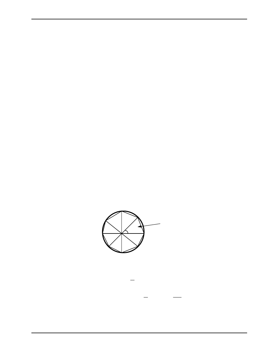
Approximation of the area of a circle:
Area of one triangle:
S
R
i
i
=
1
2
2
sin
θ
Area of the circle:
S
S
R N
N
R as N
N
i
i
N
=
=
→
→ ∞
=
∑
1
2
2
1
2
2
sin
π
π
where N = total number of triangles (elements).
R
θ
i
“Element” S
i

Lecture Notes: Introduction to Finite Element Method
Chapter 1. Introduction
© 1998 Yijun Liu, University of Cincinnati
2
Why Finite Element Method?
•
Design analysis: hand calculations, experiments, and
computer simulations
•
FEM/FEA is the most widely applied computer simulation
method in engineering
•
Closely integrated with CAD/CAM applications
•
...
Applications of FEM in Engineering
•
Mechanical/Aerospace/Civil/Automobile Engineering
•
Structure analysis (static/dynamic, linear/nonlinear)
•
Thermal/fluid flows
•
Electromagnetics
•
Geomechanics
•
Biomechanics
•
...
Examples:
...

Lecture Notes: Introduction to Finite Element Method
Chapter 1. Introduction
© 1998 Yijun Liu, University of Cincinnati
3
A Brief History of the FEM
•
1943 ----- Courant (Variational methods)
•
1956 ----- Turner, Clough, Martin and Topp (Stiffness)
•
1960 ----- Clough (“Finite Element”, plane problems)
•
1970s ----- Applications on mainframe computers
•
1980s ----- Microcomputers, pre- and postprocessors
•
1990s ----- Analysis of large structural systems

Lecture Notes: Introduction to Finite Element Method
Chapter 1. Introduction
© 1998 Yijun Liu, University of Cincinnati
4
FEM in Structural Analysis
Procedures:
•
Divide structure into pieces (elements with nodes)
•
Describe the behavior of the physical quantities on each
element
•
Connect (assemble) the elements at the nodes to form an
approximate system of equations for the whole structure
•
Solve the system of equations involving unknown
quantities at the nodes (e.g., displacements)
•
Calculate desired quantities (e.g., strains and stresses) at
selected elements
Example:

Lecture Notes: Introduction to Finite Element Method
Chapter 1. Introduction
© 1998 Yijun Liu, University of Cincinnati
5
Computer Implementations
•
Preprocessing (build FE model, loads and constraints)
•
FEA solver (assemble and solve the system of equations)
•
Postprocessing (sort and display the results)
Available Commercial FEM Software Packages
•
ANSYS (General purpose, PC and workstations)
•
SDRC/I-DEAS (Complete CAD/CAM/CAE package)
•
NASTRAN (General purpose FEA on mainframes)
•
ABAQUS (Nonlinear and dynamic analyses)
•
COSMOS (General purpose FEA)
•
ALGOR (PC and workstations)
•
PATRAN (Pre/Post Processor)
•
HyperMesh (Pre/Post Processor)
•
Dyna-3D (Crash/impact analysis)
•
...

Lecture Notes: Introduction to Finite Element Method
Chapter 1. Introduction
© 1998 Yijun Liu, University of Cincinnati
6
Objectives of This FEM Course
•
Understand the fundamental ideas of the FEM
•
Know the behavior and usage of each type of elements
covered in this course
•
Be able to prepare a suitable FE model for given problems
•
Can interpret and evaluate the quality of the results (know
the physics of the problems)
•
Be aware of the limitations of the FEM (don’t misuse the
FEM - a numerical tool)

Lecture Notes: Introduction to Finite Element Method
Chapter 1. Introduction
© 1998 Yijun Liu, University of Cincinnati
7
II. Review of Matrix Algebra
Linear System of Algebraic Equations
a x
a x
a x
b
a x
a x
a x
b
a x
a x
a x
b
n
n
n
n
n
n
nn
n
n
11
1
12
2
1
1
21
1
22
2
2
2
1
1
2
2
+
+ +
=
+
+ +
=
+
+ +
=
...
...
.......
...
(1)
where x
1
, x
2
, ..., x
n
are the unknowns.
In matrix form:
Ax
b
=
(2)
where
[ ]
{ }
{ }
A
x
b
=
=
=
=
=
=
a
a
a
a
a
a
a
a
a
a
x
x
x
x
b
b
b
b
ij
n
n
n
n
nn
i
n
i
n
11
12
1
21
22
2
1
2
1
2
1
2
...
...
...
...
...
...
...
:
:
(3)
A is called a n×n (square) matrix, and x and b are (column)
vectors of dimension n.

Lecture Notes: Introduction to Finite Element Method
Chapter 1. Introduction
© 1998 Yijun Liu, University of Cincinnati
8
Row and Column Vectors
[
]
v
w
=
=
v
v
v
w
w
w
1
2
3
1
2
3
Matrix Addition and Subtraction
For two matrices A and B, both of the same size (m×n), the
addition and subtraction are defined by
C
A
B
D
A
B
= +
=
+
= −
=
−
with
with
c
a
b
d
a
b
ij
ij
ij
ij
ij
ij
Scalar Multiplication
[ ]
λ
λ
A
=
a
ij
Matrix Multiplication
For two matrices A (of size l×m) and B (of size m×n), the
product of AB is defined by
C
AB
=
= ∑
=
with c
a b
ij
ik
k
m
kj
1
where i = 1, 2, ..., l; j = 1, 2, ..., n.
Note that, in general, AB
BA
≠
, but
(
)
(
)
AB C
A BC
=
(associative).

Lecture Notes: Introduction to Finite Element Method
Chapter 1. Introduction
© 1998 Yijun Liu, University of Cincinnati
9
Transpose of a Matrix
If A = [a
ij
], then the transpose of A is
[ ]
A
T
ji
a
=
Notice that (
)
AB
B A
T
T
T
=
.
Symmetric Matrix
A square (n×n) matrix A is called symmetric, if
A
A
=
T
or
a
a
ij
ji
=
Unit (Identity) Matrix
I
=
1
0
0
0
1
0
0
0
1
...
...
... ... ... ...
...
Note that AI = A, Ix = x.
Determinant of a Matrix
The determinant of square matrix A is a scalar number
denoted by det A or |A|. For 2×2 and 3×3 matrices, their
determinants are given by
det
a
b
c
d
ad
bc
=
−

Lecture Notes: Introduction to Finite Element Method
Chapter 1. Introduction
© 1998 Yijun Liu, University of Cincinnati
10
and
det
a
a
a
a
a
a
a
a
a
a a a
a a a
a a a
a a a
a a a
a a a
11
12
13
21
22
23
31
32
33
11 22
33
12
23 31
21 32 13
13 22
31
12
21 33
23 32 11
=
+
+
−
−
−
Singular Matrix
A square matrix A is singular if det A = 0, which indicates
problems in the systems (nonunique solutions, degeneracy, etc.)
Matrix Inversion
For a square and nonsingular matrix A ( det A
≠
0), its
inverse A
-1
is constructed in such a way that
AA
A A
I
−
−
=
=
1
1
The cofactor matrix C of matrix A is defined by
C
M
ij
i
j
ij
= −
+
(
)
1
where M
ij
is the determinant of the smaller matrix obtained by
eliminating the ith row and jth column of A.
Thus, the inverse of A can be determined by
A
A
C
−
=
1
1
det
T
We can show that (
)
AB
B A
−
−
−
=
1
1
1
.

Lecture Notes: Introduction to Finite Element Method
Chapter 1. Introduction
© 1998 Yijun Liu, University of Cincinnati
11
Examples:
(1)
a
b
c
d
ad
bc
d
b
c
a
=
−
−
−
−
1
1
(
)
Checking,
a
b
c
d
a
b
c
d
ad
bc
d
b
c
a
a
b
c
d
=
−
−
−
=
−
1
1
1
0
0
1
(
)
(2)
1
1
0
1
2
1
0
1
2
1
4 2 1
3
2 1
2
2 1
1
1 1
3 2 1
2
2 1
1
1 1
1
−
−
−
−
=
− −
=
−
(
)
T
Checking,
1
1
0
1
2
1
0
1
2
3
2 1
2
2 1
1
1 1
1
0
0
0
1
0
0
0
1
−
−
−
−
=
If det A = 0 (i.e., A is singular), then A
-1
does not exist!
The solution of the linear system of equations (Eq.(1)) can be
expressed as (assuming the coefficient matrix A is nonsingular)
x
A b
=
−
1
Thus, the main task in solving a linear system of equations is to
found the inverse of the coefficient matrix.

Lecture Notes: Introduction to Finite Element Method
Chapter 1. Introduction
© 1998 Yijun Liu, University of Cincinnati
12
Solution Techniques for Linear Systems of Equations
•
Gauss elimination methods
•
Iterative methods
Positive Definite Matrix
A square (n×n) matrix A is said to be positive definite, if for
any nonzero vector x of dimension n,
x Ax
T
>
0
Note that positive definite matrices are nonsingular.
Differentiation and Integration of a Matrix
Let
[ ]
A( )
( )
t
a t
ij
=
then the differentiation is defined by
d
dt
t
da t
dt
ij
A( )
( )
=
and the integration by
A( )
( )
t dt
a t dt
ij
=
∫
∫
Lecture Notes: Introduction to Finite Element Method
Chapter 1. Introduction
© 1998 Yijun Liu, University of Cincinnati
13
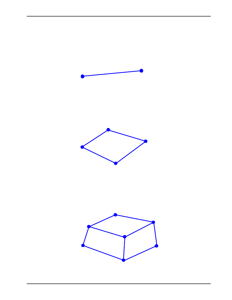
Types of Finite Elements
1-D (Line) Element
(Spring, truss, beam, pipe, etc.)
2-D (Plane) Element
(Membrane, plate, shell, etc.)
3-D (Solid) Element
(3-D fields - temperature, displacement, stress, flow velocity)
Lecture Notes: Introduction to Finite Element Method
Chapter 1. Introduction
© 1998 Yijun Liu, University of Cincinnati
14
III. Spring Element
“
Everything important is simple
.
”
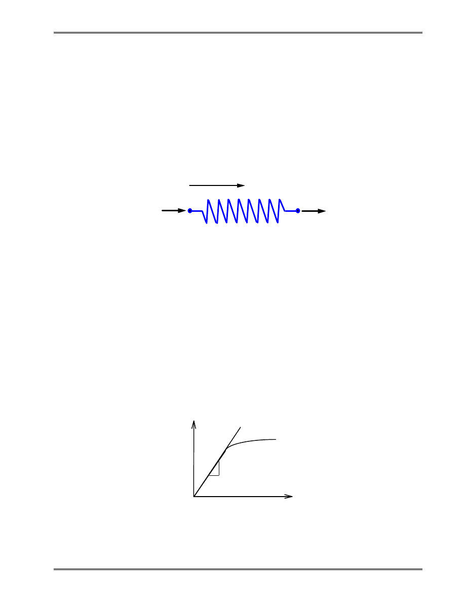
One Spring Element
Two nodes:
i, j
Nodal displacements:
u
i
, u
j
(in, m, mm)
Nodal forces:
f
i
, f
j
(lb, Newton)
Spring constant (stiffness):
k (lb/in, N/m, N/mm)
Spring force-displacement relationship:
F
k
= ∆
with
∆ =
−
u
u
j
i
k
F
=
/
∆
(> 0) is the force needed to produce a unit stretch.
k
i
j
u
j
u
i
f
i
f
j
x
∆
F
Nonlinear
Linear
k

Lecture Notes: Introduction to Finite Element Method
Chapter 1. Introduction
© 1998 Yijun Liu, University of Cincinnati
15
We only consider linear problems in this introductory
course.
Consider the equilibrium of forces for the spring. At node i,
we have
f
F
k u
u
ku
ku
i
j
i
i
j
= −
= −
−
=
−
(
)
and at node j,
f
F
k u
u
ku
ku
j
j
i
i
j
= =
−
= −
+
(
)
In matrix form,
k
k
k
k
u
u
f
f
i
j
i
j
−
−
=
or,
ku
f
=
where
k = (element) stiffness matrix
u = (element nodal) displacement vector
f = (element nodal) force vector
Note that k is symmetric. Is k singular or nonsingular? That is,
can we solve the equation? If not, why?
Lecture Notes: Introduction to Finite Element Method
Chapter 1. Introduction
© 1998 Yijun Liu, University of Cincinnati
16
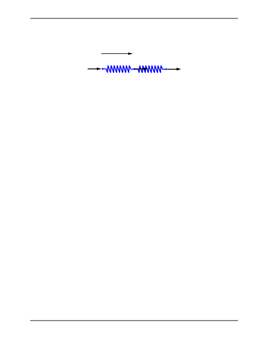
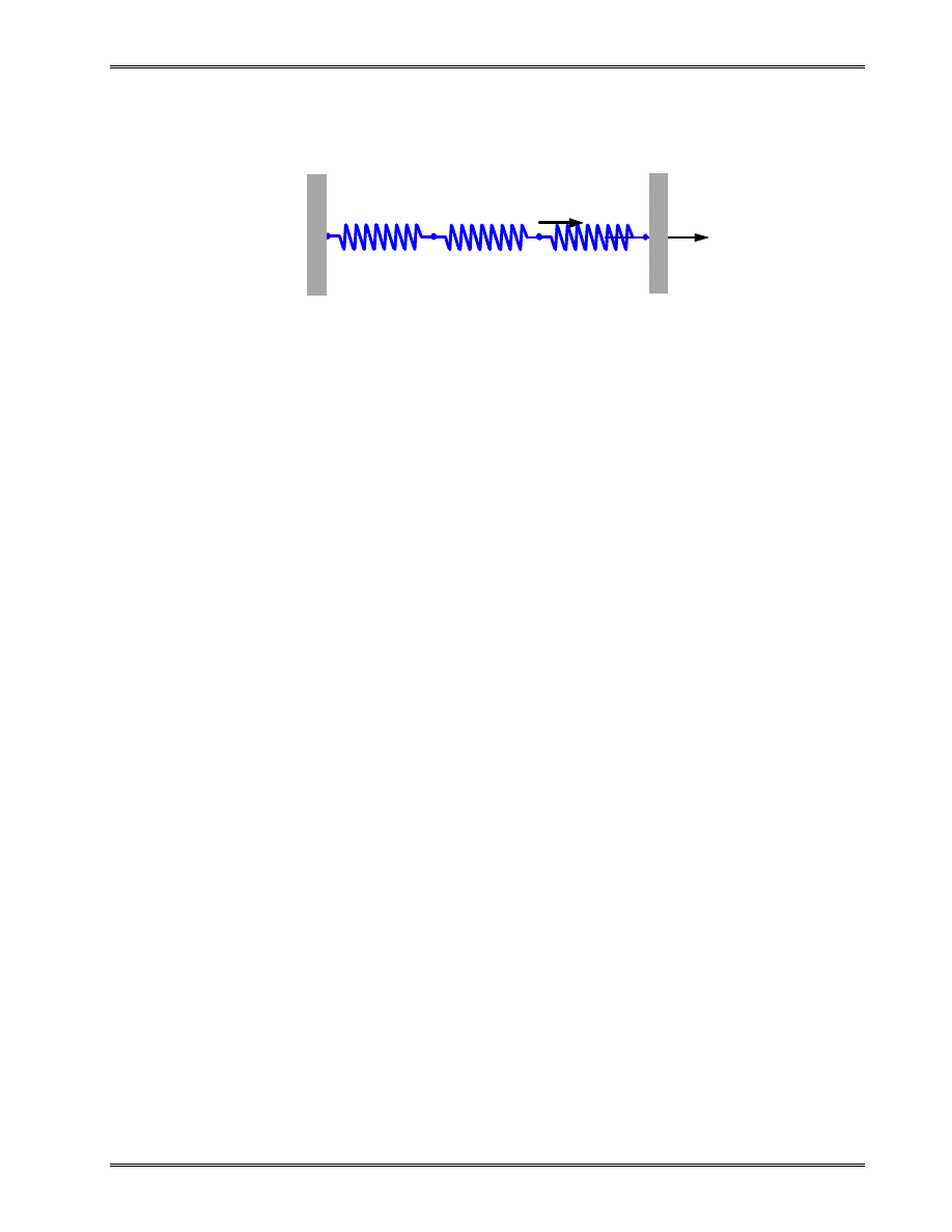
Spring System
For element 1,
k
k
k
k
u
u
f
f
1
1
1
1
1
2
1
1
2
1
−
−
=
element 2,
k
k
k
k
u
u
f
f
2
2
2
2
2
3
1
2
2
2
−
−
=
where
f
i
m
is the (internal) force acting on local node i of element
m (i = 1, 2).
Assemble the stiffness matrix for the whole system:
Consider the equilibrium of forces at node 1,
F
f
1
1
1
=
at node 2,
F
f
f
2
2
1
1
2
=
+
and node 3,
F
f
3
2
2
=
k
1
u
1,
F
1
x
k
2
u
2,
F
2
u
3,
F
3
1
2
3

Lecture Notes: Introduction to Finite Element Method
Chapter 1. Introduction
© 1998 Yijun Liu, University of Cincinnati
17
That is,
F
k u
k u
F
k u
k
k u
k u
F
k u
k u
1
1 1
1
2
2
1 1
1
2
2
2
3
3
2
2
2
3
=
−
= −
+
+
−
= −
+
(
)
In matrix form,
k
k
k
k
k
k
k
k
u
u
u
F
F
F
1
1
1
1
2
2
2
2
1
2
3
1
2
3
0
0
−
−
+
−
−
=
or
KU
F
=
K is the stiffness matrix (structure matrix) for the spring system.
An alternative way of assembling the whole stiffness matrix:
“Enlarging” the stiffness matrices for elements 1 and 2, we
have
k
k
k
k
u
u
u
f
f
1
1
1
1
1
2
3
1
1
2
1
0
0
0
0
0
0
−
−
=
0
0
0
0
0
0
2
2
2
2
1
2
3
1
2
2
2
k
k
k
k
u
u
u
f
f
−
−
=

Lecture Notes: Introduction to Finite Element Method
Chapter 1. Introduction
© 1998 Yijun Liu, University of Cincinnati
18
Adding the two matrix equations (superposition), we have
k
k
k
k
k
k
k
k
u
u
u
f
f
f
f
1
1
1
1
2
2
2
2
1
2
3
1
1
2
1
1
2
2
2
0
0
−
−
+
−
−
=
+
This is the same equation we derived by using the force
equilibrium concept.
Boundary and load conditions:
Assuming,
u
F
F
P
1
2
3
0
=
=
=
and
we have
k
k
k
k
k
k
k
k
u
u
F
P
P
1
1
1
1
2
2
2
2
2
3
1
0
0
0
−
−
+
−
−
=
which reduces to
k
k
k
k
k
u
u
P
P
1
2
2
2
2
2
3
+
−
−
=
and
F
k u
1
1
2
= −
Unknowns are
U
=
u
u
2
3
and the reaction force
F
1
(if desired).

Lecture Notes: Introduction to Finite Element Method
Chapter 1. Introduction
© 1998 Yijun Liu, University of Cincinnati
19
Solving the equations, we obtain the displacements
u
u
P k
P k
P k
2
3
1
1
2
2
2
=
+
/
/
/
and the reaction force
F
P
1
2
= −
Checking the Results
•
Deformed shape of the structure
•
Balance of the external forces
•
Order of magnitudes of the numbers
Notes About the Spring Elements
•
Suitable for stiffness analysis
•
Not suitable for stress analysis of the spring itself
•
Can have spring elements with stiffness in the lateral
direction, spring elements for torsion, etc.
Lecture Notes: Introduction to Finite Element Method
Chapter 1. Introduction
© 1998 Yijun Liu, University of Cincinnati
20
Example 1.1
Given:
For the spring system shown above,
k
k
k
P
u
1
2
3
4
0
=
=
=
=
=
=
100 N / mm,
200 N / mm,
100 N / mm
500 N, u
1
Find:
(a) the global stiffness matrix
(b) displacements of nodes 2 and 3
(c) the reaction forces at nodes 1 and 4
(d) the force in the spring 2
Solution:
(a) The element stiffness matrices are
k
1
100
100
100
100
=
−
−
(N/mm)
(1)
k
2
200
200
200
200
=
−
−
(N/mm)
(2)
k
3
100
100
100
100
=
−
−
(N/mm)
(3)
k
1
x
k
2
1
2
3
k
3
4
P
Lecture Notes: Introduction to Finite Element Method
Chapter 1. Introduction
© 1998 Yijun Liu, University of Cincinnati
21
Applying the superposition concept, we obtain the global stiffness
matrix for the spring system as
u
u
u
u
1
2
3
4
100
100
0
0
100 100 200
200
0
0
200
200 100
100
0
0
100
100
K
=
−
−
+
−
−
+
−
−
or
K
=
−
−
−
−
−
−
100
100
0
0
100
300
200
0
0
200
300
100
0
0
100
100
which is symmetric and banded.
Equilibrium (FE) equation for the whole system is
100
100
0
0
100
300
200
0
0
200
300
100
0
0
100
100
0
1
2
3
4
1
4
−
−
−
−
−
−
=
u
u
u
u
F
P
F
(4)
(b) Applying the BC (
u
u
1
4
0
=
=
) in Eq(4), or deleting the 1
st
and
4
th
rows and columns, we have

Lecture Notes: Introduction to Finite Element Method
Chapter 1. Introduction
© 1998 Yijun Liu, University of Cincinnati
22
300
200
200
300
0
2
3
−
−
=
u
u
P
(5)
Solving Eq.(5), we obtain
u
u
P
P
2
3
250
3
500
2
3
=
=
/
/
(
)
mm
(6)
(c) From the 1
st
and 4
th
equations in (4), we get the reaction forces
F
u
1
2
100
200
= −
= −
(N)
F
u
4
3
100
300
= −
= −
( )
N
(d) The FE equation for spring (element) 2 is
200
200
200
200
−
−
=
u
u
f
f
i
j
i
j
Here i = 2, j = 3 for element 2. Thus we can calculate the spring
force as
[
]
[
]
F
f
f
u
u
j
i
=
= −
= −
= −
=
200 200
200 200
2
3
200
2
3
(N)
Check the results!
Lecture Notes: Introduction to Finite Element Method
Chapter 1. Introduction
© 1998 Yijun Liu, University of Cincinnati
23
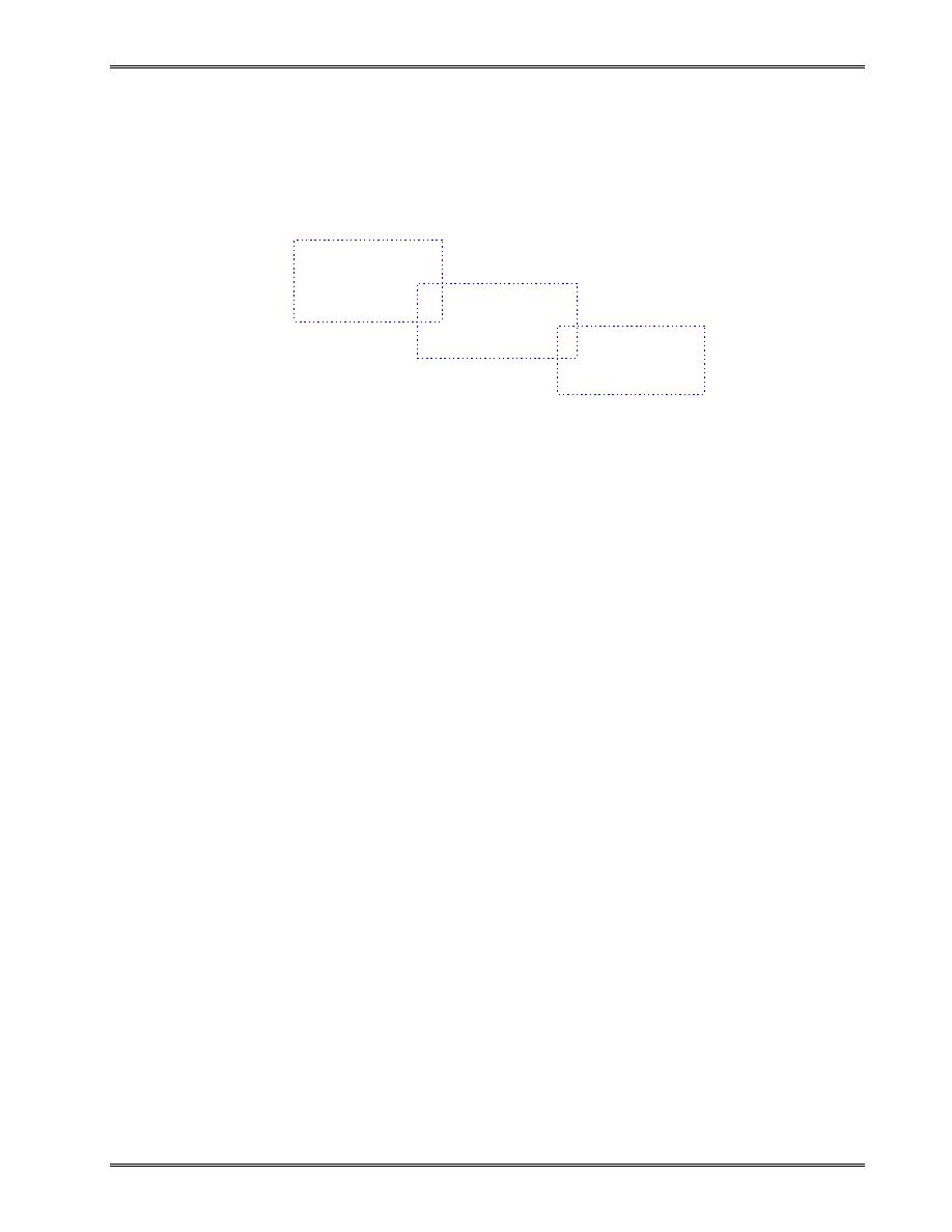
Example 1.2
Problem: For the spring system with arbitrarily numbered nodes
and elements, as shown above, find the global stiffness
matrix.
Solution:
First we construct the following
which specifies the global node numbers corresponding to the
local node numbers for each element.
Then we can write the element stiffness matrices as follows
k
1
x
k
2
4
2
3
k
3
5
F
2
F
1
k
4
1
1
2
3
4
Element Connectivity Table
Element
Node i (1)
Node j (2)
1
4
2
2
2
3
3
3
5
4
2
1

Lecture Notes: Introduction to Finite Element Method
Chapter 1. Introduction
© 1998 Yijun Liu, University of Cincinnati
24
u
u
k
k
k
k
4
2
1
1
1
1
1
k
=
−
−
u
u
k
k
k
k
2
3
2
2
2
2
2
k
=
−
−
u
u
k
k
k
k
3
5
3
3
3
3
3
k
=
−
−
u
u
k
k
k
k
2
1
4
4
4
4
4
k
=
−
−
Finally, applying the superposition method, we obtain the global
stiffness matrix as follows
u
u
u
u
u
k
k
k
k
k
k
k
k
k
k
k
k
k
k
k
k
1
2
3
4
5
4
4
4
1
2
4
2
1
2
2
3
3
1
1
3
3
0
0
0
0
0
0
0
0
0
0
0
0
K
=
−
−
+
+
−
−
−
+
−
−
−
The matrix is symmetric, banded, but singular.

Lecture Notes: Introduction to Finite Element Method
Chapter 2. Bar and Beam Elements
© 1998 Yijun Liu, University of Cincinnati
25
Chapter 2. Bar and Beam Elements.
Linear Static Analysis
I. Linear Static Analysis
Most structural analysis problems can be treated as linear
static problems, based on the following assumptions
1. Small deformations (loading pattern is not changed due
to the deformed shape)
2. Elastic materials (no plasticity or failures)
3. Static loads (the load is applied to the structure in a slow
or steady fashion)
Linear analysis can provide most of the information about
the behavior of a structure, and can be a good approximation for
many analyses. It is also the bases of nonlinear analysis in most
of the cases.
Lecture Notes: Introduction to Finite Element Method
Chapter 2. Bar and Beam Elements
© 1998 Yijun Liu, University of Cincinnati
26
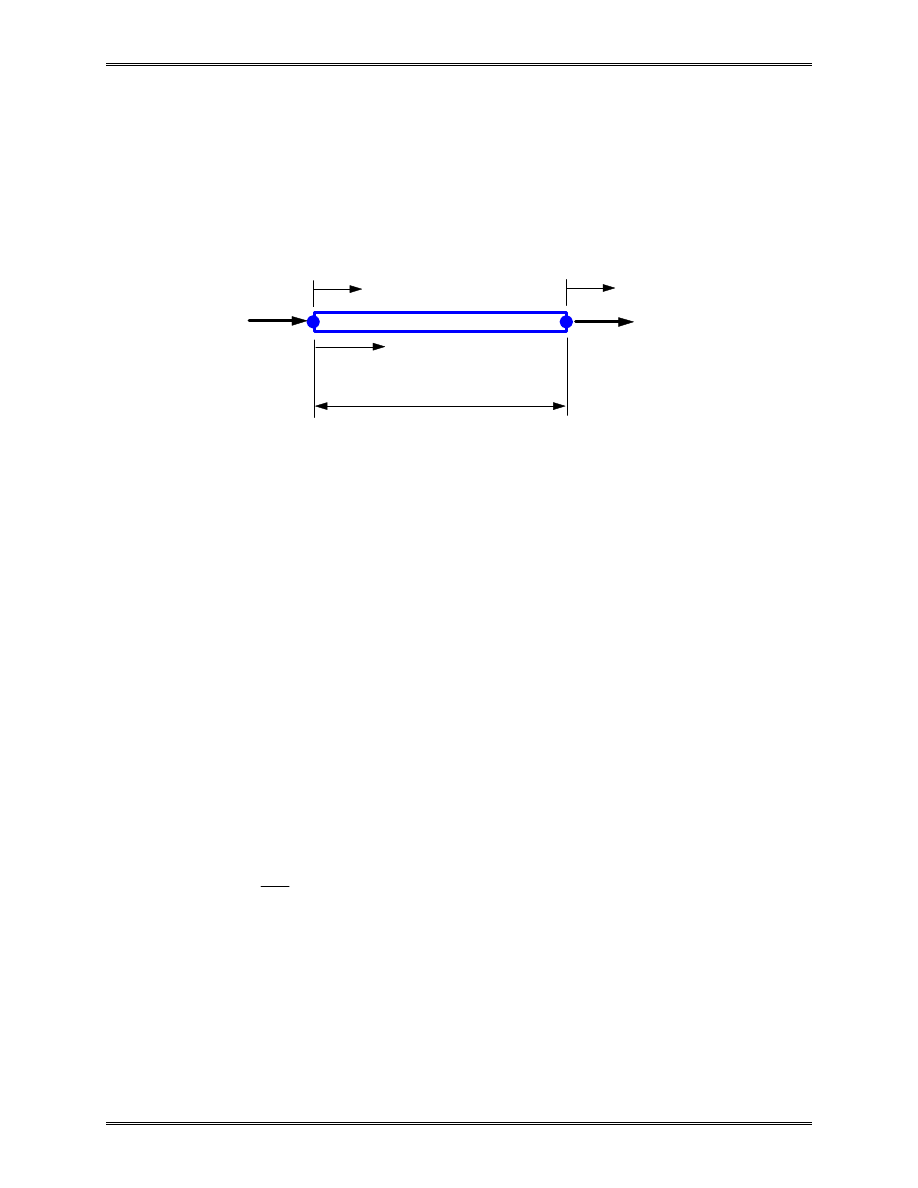
II. Bar Element
Consider a uniform prismatic bar:
L
length
A
cross-sectional area
E
elastic modulus
u
u x
=
( )
displacement
ε ε
=
( )
x
strain
σ σ
=
( )
x
stress
Strain-displacement relation:
ε
=
du
dx
(1)
Stress-strain relation:
σ
ε
=
E
(2)
L
x
f
i
i
j
f
j
u
i
u
j
A,E

Lecture Notes: Introduction to Finite Element Method
Chapter 2. Bar and Beam Elements
© 1998 Yijun Liu, University of Cincinnati
27
Stiffness Matrix --- Direct Method
Assuming that the displacement u is varying linearly along
the axis of the bar, i.e.,
u x
x
L
u
x
L
u
i
j
( )
= −
+
1
(3)
we have
ε
=
−
=
u
u
L
L
j
i
∆
(
∆
= elongation)
(4)
σ
ε
=
=
E
E
L
∆
(5)
We also have
σ
=
F
A
(F = force in bar)
(6)
Thus, (5) and (6) lead to
F
EA
L
k
=
=
∆
∆
(7)
where
k
EA
L
=
is the stiffness of the bar.
The bar is acting like a spring in this case and we conclude
that element stiffness matrix is

Lecture Notes: Introduction to Finite Element Method
Chapter 2. Bar and Beam Elements
© 1998 Yijun Liu, University of Cincinnati
28
k
=
−
−
=
−
−
k
k
k
k
EA
L
EA
L
EA
L
EA
L
or
k
=
−
−
EA
L
1
1
1
1
(8)
This can be verified by considering the equilibrium of the forces
at the two nodes.
Element equilibrium equation is
EA
L
u
u
f
f
i
j
i
j
1
1
1
1
−
−
=
(9)
Degree of Freedom (dof)
Number of components of the displacement vector at a
node.
For 1-D bar element: one dof at each node.
Physical Meaning of the Coefficients in k
The jth column of k (here j = 1 or 2) represents the forces
applied to the bar to maintain a deformed shape with unit
displacement at node j and zero displacement at the other node.

Lecture Notes: Introduction to Finite Element Method
Chapter 2. Bar and Beam Elements
© 1998 Yijun Liu, University of Cincinnati
29
Stiffness Matrix --- A Formal Approach
We derive the same stiffness matrix for the bar using a
formal approach which can be applied to many other more
complicated situations.
Define two linear shape functions as follows
N
N
i
j
( )
,
( )
ξ
ξ
ξ
ξ
= −
=
1
(10)
where
ξ
ξ
=
≤ ≤
x
L
,
0
1
(11)
From (3) we can write the displacement as
u x
u
N
u
N
u
i
i
j
j
( )
( )
( )
( )
=
=
+
ξ
ξ
ξ
or
[
]
u
N
N
u
u
i
j
i
j
=
=
Nu
(12)
Strain is given by (1) and (12) as
ε
=
=
=
du
dx
d
dx
N u
Bu
(13)
where B is the element strain-displacement matrix, which is
[
] [
]
B
=
=
•
d
dx
N
N
d
d
N
N
d
dx
i
j
i
j
( )
( )
( )
( )
ξ
ξ
ξ
ξ
ξ
ξ
i.e.,
[
]
B
= −
1
1
/
/
L
L
(14)

Lecture Notes: Introduction to Finite Element Method
Chapter 2. Bar and Beam Elements
© 1998 Yijun Liu, University of Cincinnati
30
Stress can be written as
σ
ε
=
=
E
EBu
(15)
Consider the strain energy stored in the bar
(
)
(
)
U
dV
E
dV
E
dV
V
V
V
=
=
=
∫
∫
∫
1
2
1
2
1
2
σ ε
T
T
T
T
T
u B
Bu
u
B
B
u
(16)
where (13) and (15) have been used.
The work done by the two nodal forces is
W
f u
f u
i
i
j
j
=
+
=
1
2
1
2
1
2
u f
T
(17)
For conservative system, we state that
U
W
=
(18)
which gives
(
)
1
2
1
2
u
B
B
u
u f
T
T
T
E
dV
V
∫
=
We can conclude that
(
)
B
B
u
f
T
E
dV
V
∫
=
or

Lecture Notes: Introduction to Finite Element Method
Chapter 2. Bar and Beam Elements
© 1998 Yijun Liu, University of Cincinnati
31
ku
f
=
(19)
where
(
)
k
B
B
T
=
∫
E
dV
V
(20)
is the element stiffness matrix.
Expression (20) is a general result which can be used for
the construction of other types of elements. This expression can
also be derived using other more rigorous approaches, such as
the Principle of Minimum Potential Energy, or the Galerkin’s
Method.
Now, we evaluate (20) for the bar element by using (14)
[
]
k
=
−
−
=
−
−
∫
1
1
1
1
1
1
1
1
0
/
/
/
/
L
L
E
L
L Adx
EA
L
L
which is the same as we derived using the direct method.
Note that from (16) and (20), the strain energy in the
element can be written as
U
=
1
2
u ku
T
(21)
Lecture Notes: Introduction to Finite Element Method
Chapter 2. Bar and Beam Elements
© 1998 Yijun Liu, University of Cincinnati
32
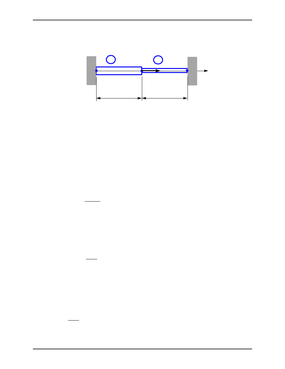
Example 2.1
Problem: Find the stresses in the two bar assembly which is
loaded with force P, and constrained at the two ends,
as shown in the figure.
Solution: Use two 1-D bar elements.
Element 1,
u
u
EA
L
1
2
1
2
1
1
1
1
k
=
−
−
Element 2,
u
u
EA
L
2
3
2
1
1
1
1
k
=
−
−
Imagine a frictionless pin at node 2, which connects the two
elements. We can assemble the global FE equation as follows,
EA
L
u
u
u
F
F
F
2
2
0
2
3
1
0
1
1
1
2
3
1
2
3
−
−
−
−
=
L
x
1
P
2A,E
L
2
3
A,E
1
2

Lecture Notes: Introduction to Finite Element Method
Chapter 2. Bar and Beam Elements
© 1998 Yijun Liu, University of Cincinnati
33
Load and boundary conditions (BC) are,
u
u
F
P
1
3
2
0
=
=
=
,
FE equation becomes,
EA
L
u
F
P
F
2
2
0
2
3
1
0
1
1
0
0
2
1
3
−
−
−
−
=
Deleting the 1
st
row and column, and the 3
rd
row and column,
we obtain,
[]
{ } { }
EA
L
u
P
3
2
=
Thus,
u
PL
EA
2
3
=
and
u
u
u
PL
EA
1
2
3
3
0
1
0
=
Stress in element 1 is
[
]
σ
ε
1
1
1
1
1
2
2
1
1
1
3
0
3
=
=
=
−
=
−
=
−
=
E
E
E
L
L
u
u
E
u
u
L
E
L
PL
EA
P
A
B u
/
/

Lecture Notes: Introduction to Finite Element Method
Chapter 2. Bar and Beam Elements
© 1998 Yijun Liu, University of Cincinnati
34
Similarly, stress in element 2 is
[
]
σ
ε
2
2
2
2
2
3
3
2
1
1
0
3
3
=
=
=
−
=
−
=
−
= −
E
E
E
L
L
u
u
E
u
u
L
E
L
PL
EA
P
A
B u
/
/
which indicates that bar 2 is in compression.
Check the results!
Notes:
•
In this case, the calculated stresses in elements 1 and 2
are exact within the linear theory for 1-D bar structures.
It will not help if we further divide element 1 or 2 into
smaller finite elements.
•
For tapered bars, averaged values of the cross-sectional
areas should be used for the elements.
•
We need to find the displacements first in order to find
the stresses, since we are using the displacement based
FEM.
Lecture Notes: Introduction to Finite Element Method
Chapter 2. Bar and Beam Elements
© 1998 Yijun Liu, University of Cincinnati
35
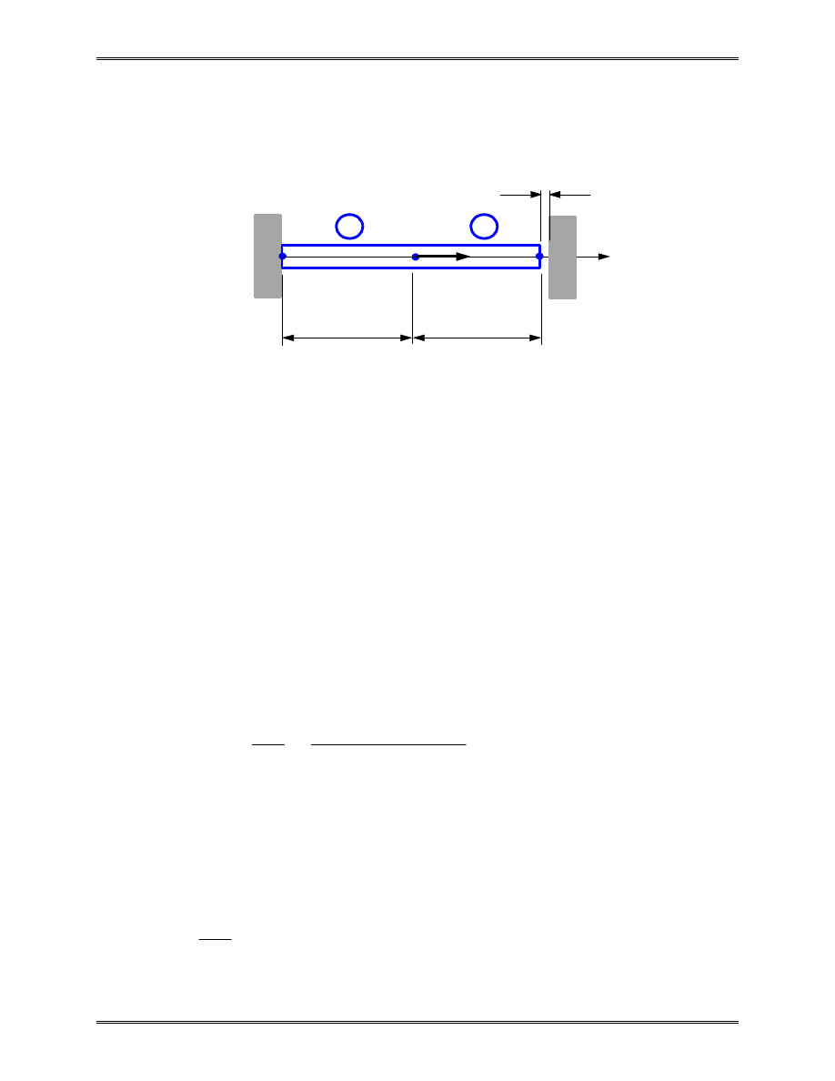
Example 2.2
Problem: Determine the support reaction forces at the two ends
of the bar shown above, given the following,
P
E
A
L
=
=
×
=
×
=
=
6 0 10
2 0 10
250
150
4
4
2
.
,
.
,
,
N
N / mm
mm
mm,
1.2 mm
2
∆
Solution:
We first check to see if or not the contact of the bar with
the wall on the right will occur. To do this, we imagine the wall
on the right is removed and calculate the displacement at the
right end,
∆
∆
0
4
4
6 0 10
150
2 0 10
250
18
12
=
=
×
×
=
> =
PL
EA
( .
)(
)
( .
)(
)
.
.
mm
mm
Thus, contact occurs.
The global FE equation is found to be,
EA
L
u
u
u
F
F
F
1
1
0
1
2
1
0
1
1
1
2
3
1
2
3
−
−
−
−
=
L
x
1
P
A,E
L
2
3
1
2
∆

Lecture Notes: Introduction to Finite Element Method
Chapter 2. Bar and Beam Elements
© 1998 Yijun Liu, University of Cincinnati
36
The load and boundary conditions are,
F
P
u
u
2
4
1
3
6 0 10
0
1 2
= =
×
=
= =
.
,
.
N
mm
∆
FE equation becomes,
EA
L
u
F
P
F
1
1
0
1
2
1
0
1
1
0
2
1
3
−
−
−
−
=
∆
The 2
nd
equation gives,
[
]
{ }
EA
L
u
P
2
1
2
−
=
∆
that is,
[]
{ }
EA
L
u
P
EA
L
2
2
=
+
∆
Solving this, we obtain
u
PL
EA
2
1
2
15
=
+
=
∆
. mm
and
u
u
u
1
2
3
0
15
12
=
.
.
(
)
mm

Lecture Notes: Introduction to Finite Element Method
Chapter 2. Bar and Beam Elements
© 1998 Yijun Liu, University of Cincinnati
37
To calculate the support reaction forces, we apply the 1
st
and 3
rd
equations in the global FE equation.
The 1
st
equation gives,
[
]
(
)
F
EA
L
u
u
u
EA
L
u
1
1
2
3
2
4
1
1 0
5 0
10
=
−
=
−
= −
×
.
N
and the 3
rd
equation gives,
[
]
(
)
F
EA
L
u
u
u
EA
L
u
u
3
1
2
3
2
3
4
0
1 1
10
10
=
−
=
−
+
= −
×
.
N
Check the results.!
Lecture Notes: Introduction to Finite Element Method
Chapter 2. Bar and Beam Elements
© 1998 Yijun Liu, University of Cincinnati
38
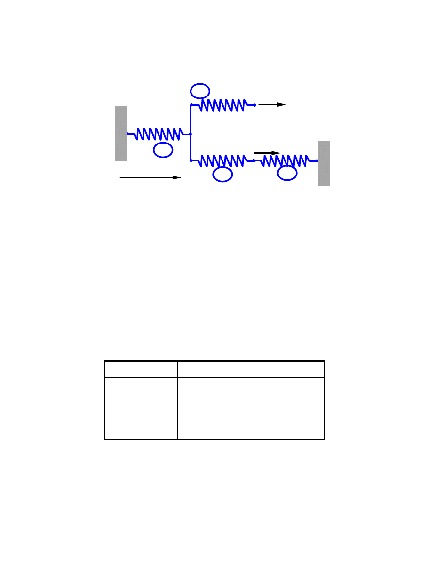
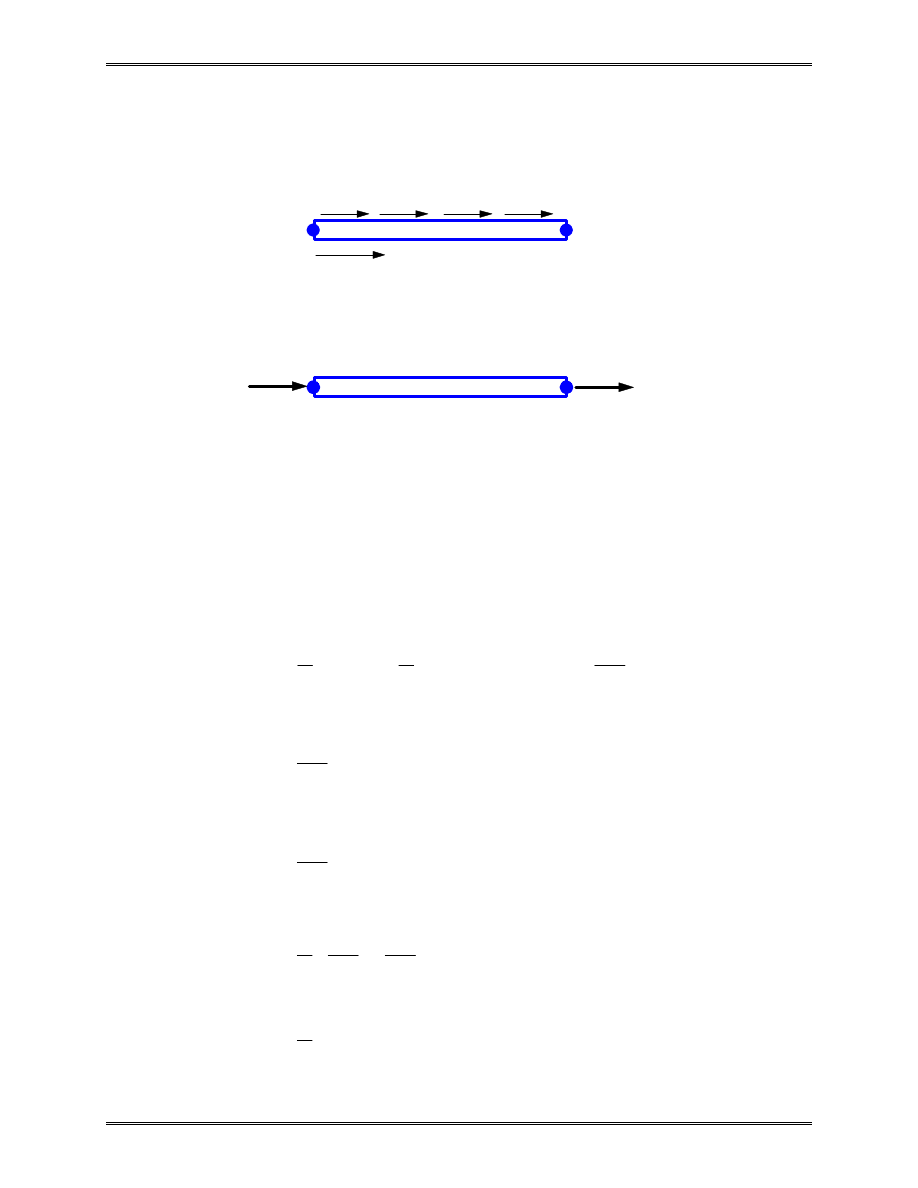
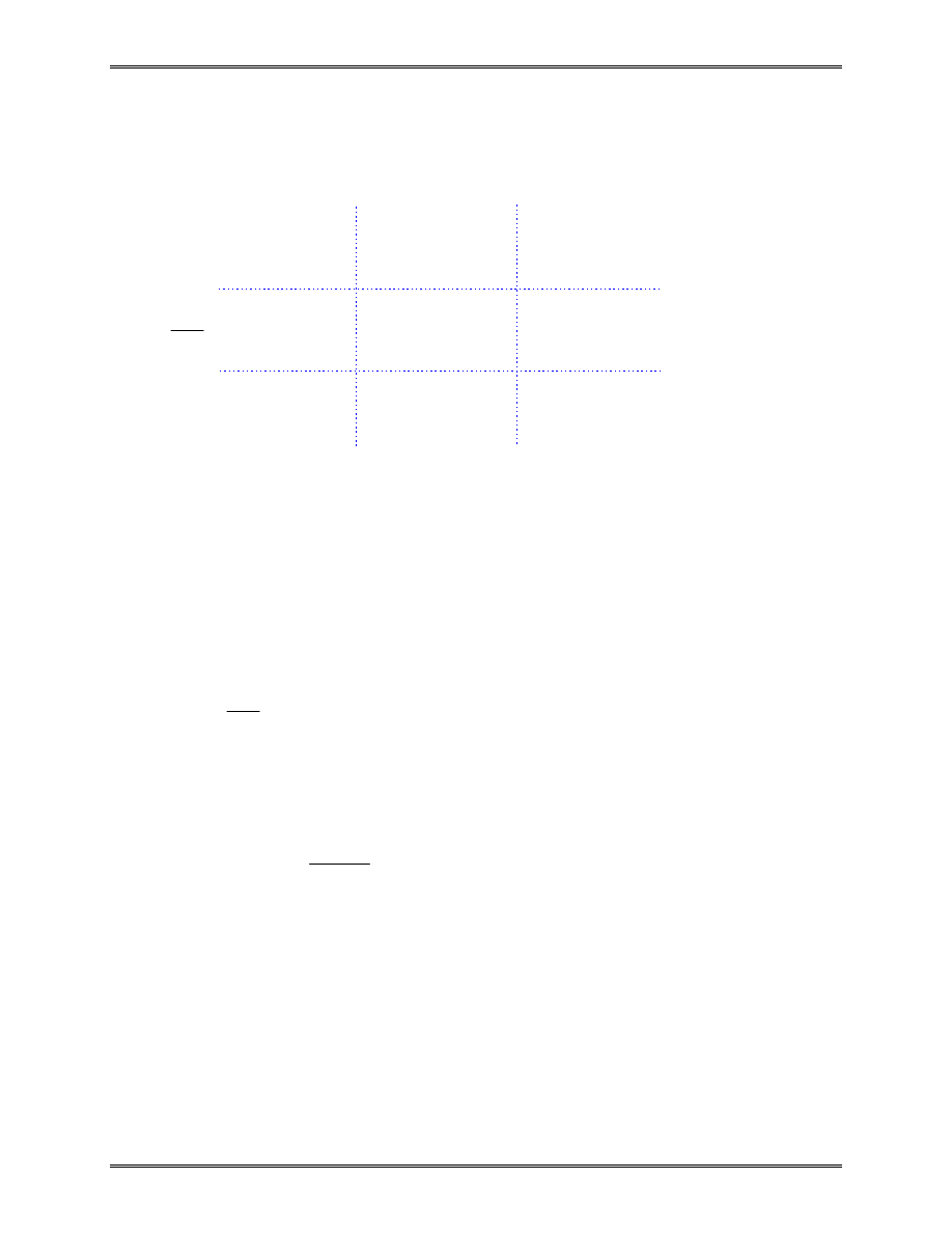
Distributed Load
Uniformly distributed axial load q (N/mm, N/m, lb/in) can
be converted to two equivalent nodal forces of magnitude qL/2.
We verify this by considering the work done by the load q,
[
]
[
]
[
]
W
uqdx
u
q Ld
qL
u
d
qL
N
N
u
u
d
qL
d
u
u
qL
qL
u
u
u
u
qL
qL
q
L
i
j
i
j
i
j
i
j
i
j
=
=
=
=
=
−
=
=
∫
∫
∫
∫
∫
1
2
1
2
2
2
2
1
1
2
2
2
1
2
2
2
0
0
1
0
1
0
1
0
1
( ) (
)
( )
( )
( )
/
/
ξ
ξ
ξ ξ
ξ
ξ
ξ
ξ ξ ξ
x
i
j
q
qL/2
i
j
qL/2
Lecture Notes: Introduction to Finite Element Method
Chapter 2. Bar and Beam Elements
© 1998 Yijun Liu, University of Cincinnati
39
that is,
W
qL
qL
q
T
q
q
=
=
1
2
2
2
u f
f
with
/
/
(22)
Thus, from the U=W concept for the element, we have
1
2
1
2
1
2
u ku
u f
u f
T
T
T
q
=
+
(23)
which yields
ku
f
f
= +
q
(24)
The new nodal force vector is
f
f
+
=
+
+
q
i
j
f
qL
f
qL
/
/
2
2
(25)
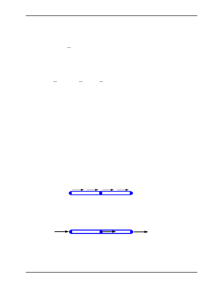
In an assembly of bars,
1
3
q
qL/2
1
3
qL/2
2
2
qL
Lecture Notes: Introduction to Finite Element Method
Chapter 2. Bar and Beam Elements
© 1998 Yijun Liu, University of Cincinnati
40
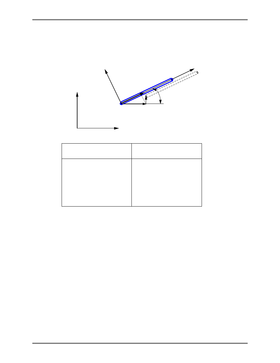
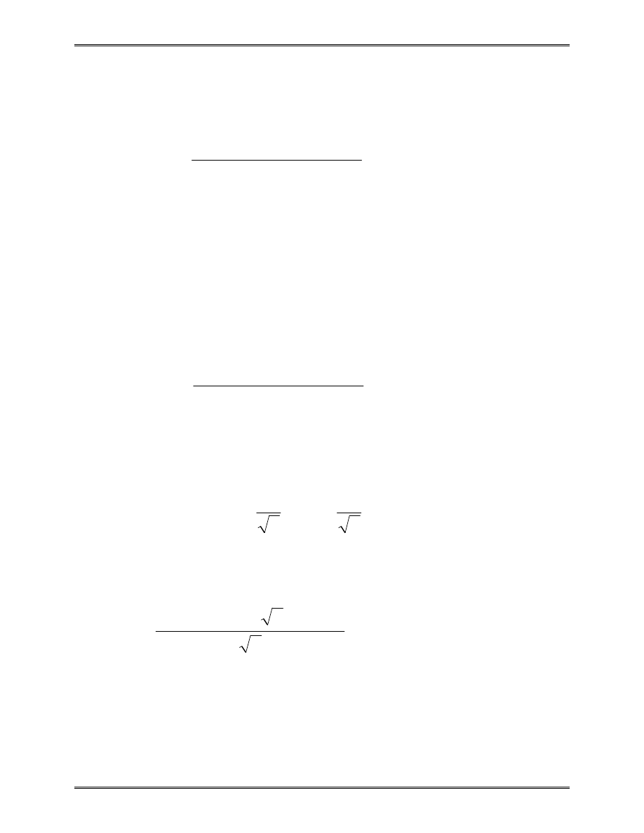
Bar Elements in 2-D and 3-D Space
2-D Case
Local
Global
x, y
X, Y
u v
i
i
'
'
,
u v
i
i
,
1 dof at node
2 dof’s at node
Note: Lateral displacement v
i
’
does not contribute to the stretch
of the bar, within the linear theory.
Transformation
[
]
[
]
u
u
v
l
m
u
v
v
u
v
m
l
u
v
i
i
i
i
i
i
i
i
i
i
'
'
cos
sin
sin
cos
=
+
=
= −
+
= −
θ
θ
θ
θ
where
l
m
=
=
cos ,
sin
θ
θ .
x
i
j
u
i
’
y
X
Y
θ
u
i
v
i

Lecture Notes: Introduction to Finite Element Method
Chapter 2. Bar and Beam Elements
© 1998 Yijun Liu, University of Cincinnati
41
In matrix form,
u
v
l
m
m
l
u
v
i
i
i
i
'
'
=
−
(26)
or,
u
Tu
i
i
'
~
=
where the transformation matrix
~
T
=
−
l
m
m
l
(27)
is orthogonal, that is,
~
~
T
T
−
=
1
T
.
For the two nodes of the bar element, we have
u
v
u
v
l
m
m
l
l
m
m
l
u
v
u
v
i
i
j
j
i
i
j
j
'
'
'
'
=
−
−
0
0
0
0
0
0
0
0
(28)
or,
u
Tu
'
=
with
T
T
0
0
T
=
~
~
(29)
The nodal forces are transformed in the same way,
f
Tf
'
=
(30)

Lecture Notes: Introduction to Finite Element Method
Chapter 2. Bar and Beam Elements
© 1998 Yijun Liu, University of Cincinnati
42
Stiffness Matrix in the 2-D Space
In the local coordinate system, we have
EA
L
u
u
f
f
i
j
i
j
1
1
1
1
−
−
=
'
'
'
'
Augmenting this equation, we write
EA
L
u
v
u
v
f
f
i
i
j
j
i
j
1
0
1 0
0
0
0
0
1 0
1
0
0
0
0
0
0
0
−
−
=
'
'
'
'
'
'
or,
k u
f
'
'
'
=
Using transformations given in (29) and (30), we obtain
k Tu
Tf
'
=
Multiplying both sides by T
T
and noticing that T
T
T = I, we
obtain
T k Tu
f
T
'
=
(31)
Thus, the element stiffness matrix k in the global coordinate
system is
k
T k T
=
T
'
(32)
which is a 4
×
4 symmetric matrix.

Lecture Notes: Introduction to Finite Element Method
Chapter 2. Bar and Beam Elements
© 1998 Yijun Liu, University of Cincinnati
43
Explicit form,
u
v
u
v
EA
L
l
lm
l
lm
lm
m
lm
m
l
lm
l
lm
lm
m
lm
m
i
i
j
j
k
=
−
−
−
−
−
−
−
−
2
2
2
2
2
2
2
2
(33)
Calculation of the directional cosines l and m:
l
X
X
L
m
Y
Y
L
j
i
j
i
=
=
−
=
=
−
cos
,
sin
θ
θ
(34)
The structure stiffness matrix is assembled by using the element
stiffness matrices in the usual way as in the 1-D case.
Element Stress
σ
ε
=
=
=
−
E
E
u
u
E
L
L
l
m
l
m
u
v
u
v
i
j
i
i
j
j
B
'
'
1
1
0
0
0
0
That is,
[
]
σ
=
−
−
E
L
l
m
l
m
u
v
u
v
i
i
j
j
(35)
Lecture Notes: Introduction to Finite Element Method
Chapter 2. Bar and Beam Elements
© 1998 Yijun Liu, University of Cincinnati
44
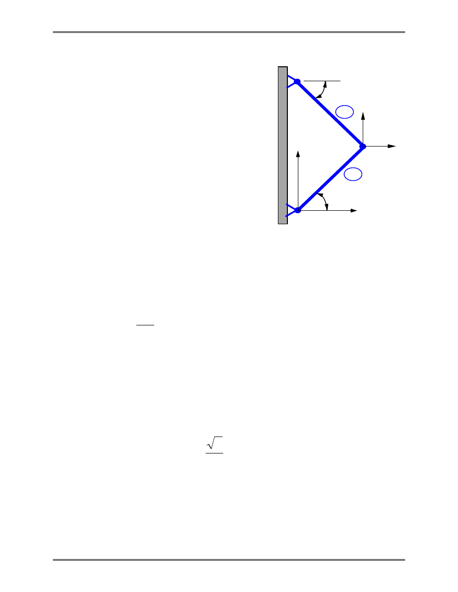
Example 2.3
A simple plane truss is made
of two identical bars (with E, A, and
L), and loaded as shown in the
figure. Find
1) displacement of node 2;
2) stress in each bar.
Solution:
This simple structure is used
here to demonstrate the assembly
and solution process using the bar element in 2-D space.
In local coordinate systems, we have
k
k
1
2
1
1
1
1
'
'
=
−
−
=
EA
L
These two matrices cannot be assembled together, because they
are in different coordinate systems. We need to convert them to
global coordinate system OXY.
Element 1:
θ
=
= =
45
2
2
o
l
m
,
Using formula (32) or (33), we obtain the stiffness matrix in the
global system
X
Y
P
1
P
2
45
o
45
o
3
2
1
1
2

Lecture Notes: Introduction to Finite Element Method
Chapter 2. Bar and Beam Elements
© 1998 Yijun Liu, University of Cincinnati
45
u
v
u
v
EA
L
T
1
1
2
2
1
1
1
1
2
1
1
1
1
1
1
1
1
1
1
1
1
1
1
1
1
k
T k T
=
=
−
−
−
−
−
−
−
−
'
Element 2:
θ
=
= −
=
135
2
2
2
2
o
l
m
,
,
We have,
u
v
u
v
EA
L
T
2
2
3
3
2
2
2
2
2
1
1
1
1
1
1
1
1
1
1
1
1
1
1
1
1
k
T k T
=
=
−
−
−
−
−
−
−
−
'
Assemble the structure FE equation,
u
v
u
v
u
v
EA
L
u
v
u
v
u
v
F
F
F
F
F
F
X
Y
X
Y
X
Y
1
1
2
2
3
3
1
1
2
2
3
3
1
1
2
2
3
3
2
1
1
1
1
0
0
1
1
1
1
0
0
1
1
2
0
1
1
1
1
0
2
1
1
0
0
1
1
1
1
0
0
1
1
1
1
−
−
−
−
−
−
−
−
−
−
−
−
−
−
=
Lecture Notes: Introduction to Finite Element Method
Chapter 2. Bar and Beam Elements
© 1998 Yijun Liu, University of Cincinnati
46
Load and boundary conditions (BC):
u
v
u
v
F
P
F
P
X
Y
1
1
3
3
2
1
2
2
0
= =
=
=
=
=
,
,
Condensed FE equation,
EA
L
u
v
P
P
2
2
0
0
2
2
2
1
2
=
Solving this, we obtain the displacement of node 2,
u
v
L
EA
P
P
2
2
1
2
=
Using formula (35), we calculate the stresses in the two bars,
[
]
(
)
σ
1
1
2
1
2
2
2
1
1 1 1
0
0
2
2
=
−
−
=
+
E
L
L
EA P
P
A
P
P
[
]
(
)
σ
2
1
2
1
2
2
2
1
1
1 1
0
0
2
2
=
−
−
=
−
E
L
L
EA
P
P
A
P
P
Check the results:
Look for the equilibrium conditions, symmetry,
antisymmetry, etc.
Lecture Notes: Introduction to Finite Element Method
Chapter 2. Bar and Beam Elements
© 1998 Yijun Liu, University of Cincinnati
47
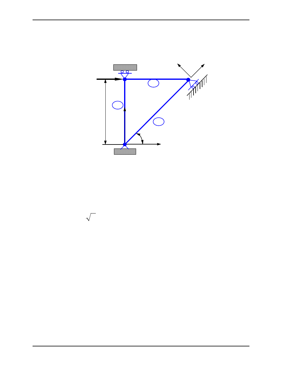
Example 2.4 (Multipoint Constraint)
For the plane truss shown above,
P
L
m
E
GPa
A
m
A
m
=
=
=
=
×
=
×
−
−
1000
1
210
6 0 10
6 2 10
4
2
4
2
kN,
for elements 1 and 2,
for element 3.
,
,
.
Determine the displacements and reaction forces.
Solution:
We have an inclined roller at node 3, which needs special
attention in the FE solution. We first assemble the global FE
equation for the truss.
Element 1:
θ
=
=
=
90
0
1
o
l
m
,
,
X
Y
P
45
o
3
2
1
3
2
1
x
’
y
’
L
Lecture Notes: Introduction to Finite Element Method
Chapter 2. Bar and Beam Elements
© 1998 Yijun Liu, University of Cincinnati
48
u
v
u
v
1
1
2
2
1
9
4
210 10
6 0 10
1
0
0
0
0
0
1
0
1
0
0
0
0
0
1 0
1
k
=
×
×
−
−
−
(
)( .
)
(
)
N / m
Element 2:
θ
=
=
=
0
1
0
o
l
m
,
,
u
v
u
v
2
2
3
3
2
9
4
210 10
6 0 10
1
1
0
1 0
0
0
0
0
1 0
1
0
0
0
0
0
k
=
×
×
−
−
−
(
)( .
)
(
)
N / m
Element 3:
θ
=
=
=
45
1
2
1
2
o
l
m
,
,
u
v
u
v
1
1
3
3
3
9
4
210
10
6 2
10
2
0 5
0 5
0 5
0 5
0 5
0 5
0 5
0 5
0 5
0 5
0 5
0 5
0 5
0 5
0 5
0 5
k
=
×
×
−
−
−
−
−
−
−
−
−
(
)(
)
.
.
.
.
.
.
.
.
.
.
.
.
.
.
.
.
(
)
N / m

Lecture Notes: Introduction to Finite Element Method
Chapter 2. Bar and Beam Elements
© 1998 Yijun Liu, University of Cincinnati
49
The global FE equation is,
1260 10
0 5
0 5 0
0
0 5
0 5
15
0
1
0 5
0 5
1
0
1
0
1
0
0
15
0 5
0 5
5
1
1
2
2
3
3
1
1
2
2
3
3
×
−
−
−
−
−
−
=
.
.
.
.
.
.
.
.
.
.
Sym.
u
v
u
v
u
v
F
F
F
F
F
F
X
Y
X
Y
X
Y
Load and boundary conditions (BC):
u
v
v
v
F
P
F
X
x
1
1
2
3
2
3
0
0
0
= =
=
=
=
=
,
,
,
.
'
'
and
From the transformation relation and the BC, we have
v
u
v
u
v
3
3
3
3
3
2
2
2
2
2
2
0
'
(
)
,
= −
=
−
+
=
that is,
u
v
3
3
0
−
=
This is a multipoint constraint (MPC).
Similarly, we have a relation for the force at node 3,
F
F
F
F
F
x
X
Y
X
Y
3
3
3
3
3
2
2
2
2
2
2
0
'
(
)
,
=
=
+
=
that is,
F
F
X
Y
3
3
0
+
=

Lecture Notes: Introduction to Finite Element Method
Chapter 2. Bar and Beam Elements
© 1998 Yijun Liu, University of Cincinnati
50
Applying the load and BC’s in the structure FE equation by
‘deleting’ 1
st
, 2
nd
and 4
th
rows and columns, we have
1260 10
1
1
0
1 15
0 5
0
0 5 0 5
5
2
3
3
3
3
×
−
−
=
.
.
.
.
u
u
v
P
F
F
X
Y
Further, from the MPC and the force relation at node 3, the
equation becomes,
1260 10
1
1
0
1 15
0 5
0
0 5 0 5
5
2
3
3
3
3
×
−
−
=
−
.
.
.
.
u
u
u
P
F
F
X
X
which is
1260 10
1
1
1
2
0
1
5
2
3
3
3
×
−
−
=
−
u
u
P
F
F
X
X
The 3
rd
equation yields,
F
u
X
3
5
3
1260 10
= −
×
Substituting this into the 2
nd
equation and rearranging, we have
1260 10
1
1
1
3
0
5
2
3
×
−
−
=
u
u
P
Solving this, we obtain the displacements,

Lecture Notes: Introduction to Finite Element Method Chapter 2. Bar and Beam Elements
© 1998 Yijun Liu, University of Cincinnati 51
u
u
P
P
2
3
5
1
2520
10
3 0 01191
0 003968
=
×
=
.
.
( )
m
From the global FE equation, we can calculate the reaction
forces,
F
F
F
F
F
u
u
v
X
Y
Y
X
Y
1
1
2
3
3
5
2
3
3
1260 10
0 0 5 0 5
0 0 5 0 5
0 0 0
1 15 0 5
0 0 5 0 5
500
500
0 0
500
500
= ×
− −
− −
−
=
−
−
−
. .
. .
. .
. .
. ( )
kN
Check the results!
A general multipoint constraint (MPC) can be described as,
A u
j j
j
=
∑
0
where A
j
’s are constants and u
j
’s are nodal displacement
components. In the FE software, such as MSC/NASTRAN,
users only need to specify this relation to the software. The
software will take care of the solution.
Penalty Approach for Handling BC’s and MPC’s
Lecture Notes: Introduction to Finite Element Method
Chapter 2. Bar and Beam Elements
© 1998 Yijun Liu, University of Cincinnati
52
3-D Case
Local
Global
x, y, z
X, Y, Z
u v
w
i
i
i
'
'
'
, ,
u v w
i
i
i
, ,
1 dof at node
3 dof’s at node
Element stiffness matrices are calculated in the local
coordinate systems and then transformed into the global
coordinate system (X, Y, Z) where they are assembled.
FEA software packages will do this transformation
automatically.
Input data for bar elements:
•
(X, Y, Z) for each node
•
E and A for each element
x
i
j
y
X
Y
Z
z
Lecture Notes: Introduction to Finite Element Method
Chapter 2. Bar and Beam Elements
© 1998 Yijun Liu, University of Cincinnati
53
III. Beam Element
Simple Plane Beam Element
L
length
I
moment of inertia of the cross-sectional area
E
elastic modulus
v
v x
=
( )
deflection (lateral displacement) of the
neutral axis
θ
=
dv
dx
rotation about the z-axis
F
F x
=
( )
shear force
M
M x
=
( )
moment about z-axis
Elementary Beam Theory:
EI
d v
dx
M x
2
2
=
( )
(36)
σ
= −
My
I
(37)
L
x
i
j
v
j
, F
j
E,I
θ
i
, M
i
θ
j
, M
j
v
i
, F
i
y

Lecture Notes: Introduction to Finite Element Method
Chapter 2. Bar and Beam Elements
© 1998 Yijun Liu, University of Cincinnati
54
Direct Method
Using the results from elementary beam theory to compute
each column of the stiffness matrix.
(Fig. 2.3-1. on Page 21 of Cook’s Book)
Element stiffness equation (local node: i, j or 1, 2):
v
v
EI
L
L
L
L
L
L
L
L
L
L
L
L
L
v
v
F
M
F
M
i
i
j
j
i
i
j
j
i
i
j
j
θ
θ
θ
θ
3
2
2
2
2
12
6
12
6
6
4
6
2
12
6
12
6
6
2
6
4
−
−
−
−
−
−
=
(38)

Lecture Notes: Introduction to Finite Element Method
Chapter 2. Bar and Beam Elements
© 1998 Yijun Liu, University of Cincinnati
55
Formal Approach
Apply the formula,
k
B
B
=
∫
T
L
EI dx
0
(39)
To derive this, we introduce the shape functions,
N x
x
L
x
L
N
x
x
x
L
x
L
N x
x
L
x
L
N
x
x
L
x
L
1
2
2
3
3
2
2
3
2
3
2
2
3
3
4
2
3
2
1 3
2
2
3
2
( )
/
/
( )
/
/
( )
/
/
( )
/
/
= −
+
= −
+
=
−
= −
+
(40)
Then, we can represent the deflection as,
[
]
v x
N x
N
x
N x
N
x
v
v
i
i
j
j
( )
( )
( )
( )
( )
=
=
Nu
1
2
3
4
θ
θ
(41)
which is a cubic function. Notice that,
N
N
N
N L
N
x
1
3
2
3
4
1
+
=
+
+
=
which implies that the rigid body motion is represented by the
assumed deformed shape of the beam.

Lecture Notes: Introduction to Finite Element Method
Chapter 2. Bar and Beam Elements
© 1998 Yijun Liu, University of Cincinnati
56
Curvature of the beam is,
d v
dx
d
dx
2
2
2
2
=
=
Nu
Bu
(42)
where the strain-displacement matrix B is given by,
[
]
B
N
=
=
= −
+
−
+
−
−
+
d
dx
N
x
N
x
N
x
N
x
L
x
L
L
x
L
L
x
L
L
x
L
2
2
1
2
3
4
2
3
2
2
3
2
6
12
4
6
6
12
2
6
"
"
"
"
( )
( )
( )
( )
(43)
Strain energy stored in the beam element is
( ) ( )
U
dV
My
I
E
My
I
dAdx
M
EI
Mdx
d v
dx
EI
d v
dx
dx
EI
dx
EI dx
T
V
A
L
T
T
L
T
L
T
L
T
T
L
=
=
−
−
=
=
=
=
∫
∫
∫
∫
∫
∫
∫
1
2
1
2
1
1
2
1
1
2
1
2
1
2
0
0
2
2
2
2
0
0
0
σ ε
Bu
Bu
u
B
B
u
We conclude that the stiffness matrix for the simple beam
element is
k
B
B
=
∫
T
L
EI dx
0

Lecture Notes: Introduction to Finite Element Method
Chapter 2. Bar and Beam Elements
© 1998 Yijun Liu, University of Cincinnati
57
Applying the result in (43) and carrying out the integration, we
arrive at the same stiffness matrix as given in (38).
Combining the axial stiffness (bar element), we obtain the
stiffness matrix of a general 2-D beam element,
u
v
u
v
EA
L
EA
L
EI
L
EI
L
EI
L
EI
L
EI
L
EI
L
EI
L
EI
L
EA
L
EA
L
EI
L
EI
L
EI
L
EI
L
EI
L
EI
L
EI
L
EI
L
i
i
i
j
j
j
θ
θ
k
=
−
−
−
−
−
−
−
−
0
0
0
0
0
12
6
0
12
6
0
6
4
0
6
2
0
0
0
0
0
12
6
0
12
6
0
6
2
0
6
4
3
2
3
2
2
2
3
2
3
2
2
2
3-D Beam Element
The element stiffness matrix is formed in the local (2-D)
coordinate system first and then transformed into the global (3-
D) coordinate system to be assembled.
(Fig. 2.3-2. On Page 24)
Lecture Notes: Introduction to Finite Element Method
Chapter 2. Bar and Beam Elements
© 1998 Yijun Liu, University of Cincinnati
58
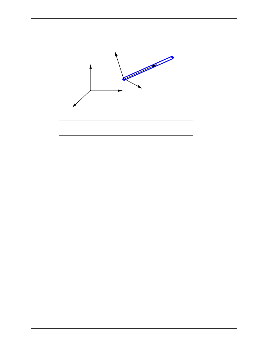
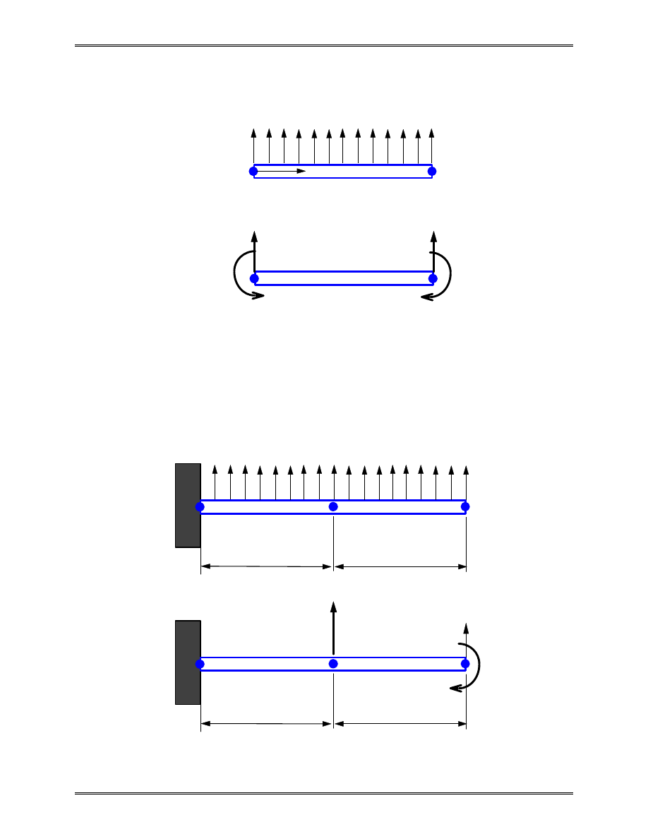
Example 2.5
Given:
The beam shown above is clamped at the two ends and
acted upon by the force P and moment M in the mid-
span.
Find:
The deflection and rotation at the center node and the
reaction forces and moments at the two ends.
Solution: Element stiffness matrices are,
v
v
EI
L
L
L
L
L
L
L
L
L
L
L
L
L
1
1
2
2
1
3
2
2
2
2
12
6
12
6
6
4
6
2
12
6
12
6
6
2
6
4
θ
θ
k
=
−
−
−
−
−
−
v
v
EI
L
L
L
L
L
L
L
L
L
L
L
L
L
2
2
3
3
2
3
2
2
2
2
12
6
12
6
6
4
6
2
12
6
12
6
6
2
6
4
θ
θ
k
=
−
−
−
−
−
−
L
X
1
2
P
E,I
Y
L
3
M
1
2
Lecture Notes: Introduction to Finite Element Method
Chapter 2. Bar and Beam Elements
© 1998 Yijun Liu, University of Cincinnati
59
Global FE equation is,
v
v
v
EI
L
L
L
L
L
L
L
L
L
L
L
L
L
L
L
L
L
L
L
L
v
v
v
F
M
F
M
F
M
Y
Y
Y
1
1
2
2
3
3
3
2
2
2
2
2
2
2
1
1
2
2
3
3
1
1
2
2
3
3
12
6
12
6
0
0
6
4
6
2
0
0
12
6
24
0
12
6
6
2
0
8
6
2
0
0
12
6
12
6
0
0
6
2
6
4
θ
θ
θ
θ
θ
θ
−
−
−
−
−
−
−
−
−
−
=
Loads and constraints (BC’s) are,
F
P
M
M
v
v
Y
2
2
1
3
1
3
0
= −
=
=
=
=
=
,
,
θ θ
Reduced FE equation,
EI
L
L
v
P
M
3
2
2
2
24
0
0
8
=
−
θ
Solving this we obtain,
v
L
EI
PL
M
2
2
2
24
3
θ
=
−
From global FE equation, we obtain the reaction forces and
moments,

Lecture Notes: Introduction to Finite Element Method
Chapter 2. Bar and Beam Elements
© 1998 Yijun Liu, University of Cincinnati
60
F
M
F
M
EI
L
L
L
L
L
L
L
v
P
M L
PL
M
P
M L
PL
M
Y
Y
1
1
3
3
3
2
2
2
2
12
6
6
2
12
6
6
2
1
4
2
3
2
3
=
−
−
−
−
=
+
+
−
−
+
θ
/
/
Stresses in the beam at the two ends can be calculated using the
formula,
σ σ
=
= −
x
My
I
Note that the FE solution is exact according to the simple beam
theory, since no distributed load is present between the nodes.
Recall that,
EI
d v
dx
M x
2
2
=
( )
and
dM
dx
V
V
dV
dx
q
q
=
=
(
(
- shear force in the beam)
- distributed load on the beam)
Thus,
EI
d v
dx
q x
4
4
=
( )
If q(x)=0, then exact solution for the deflection v is a cubic
function of x, which is what described by our shape functions.
Lecture Notes: Introduction to Finite Element Method
Chapter 2. Bar and Beam Elements
© 1998 Yijun Liu, University of Cincinnati
61
Equivalent Nodal Loads of Distributed Transverse Load
This can be verified by considering the work done by the
distributed load q.
x
i
j
q
qL/2
i
j
qL/2
L
qL
2
/12
qL
2
/12
L
q
L
L
qL
L
qL/2
qL
2
/12
Lecture Notes: Introduction to Finite Element Method
Chapter 2. Bar and Beam Elements
© 1998 Yijun Liu, University of Cincinnati
62
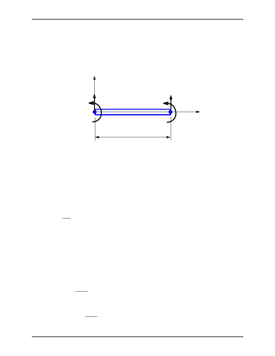
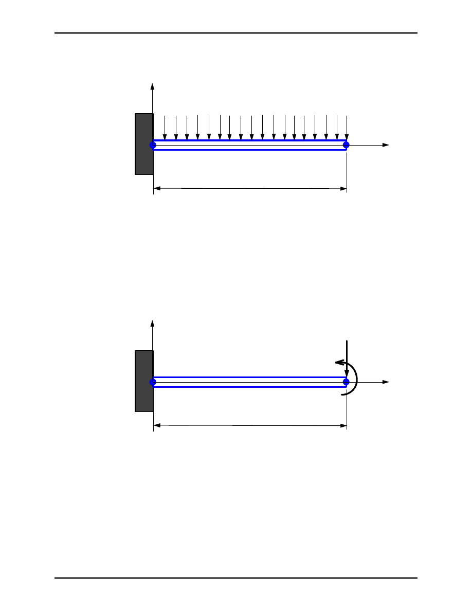
Example 2.6
Given:
A cantilever beam with distributed lateral load p as
shown above.
Find:
The deflection and rotation at the right end, the
reaction force and moment at the left end.
Solution: The work-equivalent nodal loads are shown below,
where
f
pL
m
pL
=
=
/ ,
/
2
12
2
Applying the FE equation, we have
L
x
1
2
p
E,I
y
L
x
1
2
f
E,I
y
m

Lecture Notes: Introduction to Finite Element Method
Chapter 2. Bar and Beam Elements
© 1998 Yijun Liu, University of Cincinnati
63
EI
L
L
L
L
L
L
L
L
L
L
L
L
L
v
v
F
M
F
M
Y
Y
3
2
2
2
2
1
1
2
2
1
1
2
2
12
6
12
6
6
4
6
2
12
6
12
6
6
2
6
4
−
−
−
−
−
−
=
θ
θ
Load and constraints (BC’s) are,
F
f
M
m
v
Y
2
2
1
1
0
= −
=
=
=
,
θ
Reduced equation is,
EI
L
L
L
L
v
f
m
3
2
2
2
12
6
6
4
−
−
=
−
θ
Solving this, we obtain,
v
L
EI
L f
Lm
Lf
m
pL
EI
pL
EI
2
2
2
4
3
6
2
3
3
6
8
6
θ
=
−
+
−
+
=
−
−
/
/
(A)
These nodal values are the same as the exact solution.
Note that the deflection v(x) (for 0 < x< 0) in the beam by the
FEM is, however, different from that by the exact solution. The
exact solution by the simple beam theory is a 4
th
order
polynomial of x, while the FE solution of v is only a 3
rd
order
polynomial of x.
If the equivalent moment m is ignored, we have,
v
L
EI
L f
Lf
pL
EI
pL
EI
2
2
2
4
3
6
2
3
6
4
θ
=
−
−
=
−
−
/
/
(B)

Lecture Notes: Introduction to Finite Element Method
Chapter 2. Bar and Beam Elements
© 1998 Yijun Liu, University of Cincinnati
64
The errors in (B) will decrease if more elements are used. The
equivalent moment m is often ignored in the FEM applications.
The FE solutions still converge as more elements are applied.
From the FE equation, we can calculate the reaction force
and moment as,
F
M
L
EI
L
L
L
v
pL
pL
Y
1
1
3
2
2
2
2
12
6
6
2
2
5
12
=
−
−
=
θ
/
/
where the result in (A) is used. This force vector gives the total
effective nodal forces which include the equivalent nodal forces
for the distributed lateral load p given by,
−
−
pL
pL
/
/
2
12
2
The correct reaction forces can be obtained as follows,
F
M
pL
pL
pL
pL
pL
pL
Y
1
1
2
2
2
2
5
12
2
12
2
=
−
−
−
=
/
/
/
/
/
Check the results!
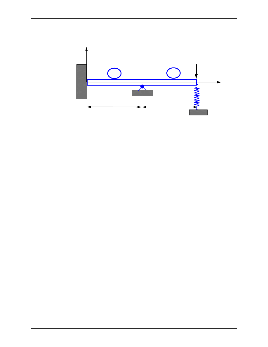
Lecture Notes: Introduction to Finite Element Method
Chapter 2. Bar and Beam Elements
© 1998 Yijun Liu, University of Cincinnati
65
Example 2.7
Given:
P = 50 kN, k = 200 kN/m, L = 3 m,
E = 210 GPa, I = 2
×
10
-4
m
4
.
Find:
Deflections, rotations and reaction forces.
Solution:
The beam has a roller (or hinge) support at node 2 and a
spring support at node 3. We use two beam elements and one
spring element to solve this problem.
The spring stiffness matrix is given by,
v
v
k
k
k
k
s
3
4
k
=
−
−
Adding this stiffness matrix to the global FE equation (see
Example 2.5), we have
L
X
1
2
P
E,I
Y
L
3
1
2
k
4

Lecture Notes: Introduction to Finite Element Method
Chapter 2. Bar and Beam Elements
© 1998 Yijun Liu, University of Cincinnati
66
v
v
v
v
EI
L
L
L
L
L
L
L
L
L
L
k
L
L
k
Symmetry
k
v
v
v
v
F
M
F
M
F
M
F
Y
Y
Y
Y
1
1
2
2
3
3
4
3
2
2
2
2
2
1
1
2
2
3
3
4
1
1
2
2
3
3
4
12
6
12
6
0
0
4
6
2
0
0
24
0
12
6
8
6
2
12
6
4
0
0
0
0
0
θ
θ
θ
θ
θ
θ
−
−
−
−
+
−
−
=
'
'
'
in which
k
L
EI
k
'
=
3
is used to simply the notation.
We now apply the boundary conditions,
v
v
v
M
M
F
P
Y
1
1
2
4
2
3
3
0
0
=
=
=
=
=
=
= −
θ
,
,
‘Deleting’ the first three and seventh equations (rows and
columns), we have the following reduced equation,
EI
L
L
L
L
L
k
L
L
L
L
v
P
3
2
2
2
2
2
3
3
8
6
2
6
12
6
2
6
4
0
0
−
−
+
−
−
= −
'
θ
θ
Solving this equation, we obtain the deflection and rotations at
node 2 and node 3,
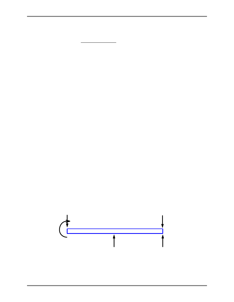
Lecture Notes: Introduction to Finite Element Method
Chapter 2. Bar and Beam Elements
© 1998 Yijun Liu, University of Cincinnati
67
θ
θ
2
3
3
2
12
7
3
7
9
v
PL
EI
k
L
= −
+
(
' )
The influence of the spring k is easily seen from this result.
Plugging in the given numbers, we can calculate
θ
θ
2
3
3
0 002492
0 01744
0 007475
v
=
−
−
−
.
.
.
rad
m
rad
From the global FE equation, we obtain the nodal reaction
forces as,
F
M
F
F
Y
Y
Y
1
1
2
4
69 78
69 78
116 2
3 488
=
−
−
⋅
.
.
.
.
kN
kN m
kN
kN
Checking the results: Draw free body diagram of the beam
1
2
50 kN
3
3.488 kN
116.2 kN
69.78 kN
69.78 kN
⋅
m
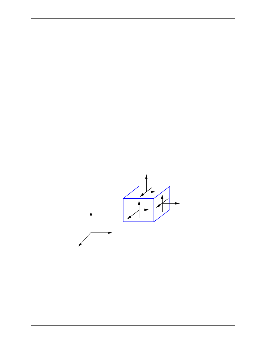
Lecture Notes: Introduction to Finite Element Method
Chapter 3. Two-Dimensional Problems
© 1998 Yijun Liu, University of Cincinnati
75
Chapter 3. Two-Dimensional Problems
I. Review of the Basic Theory
In general, the stresses and strains in a structure consist of
six components:
σ σ σ τ τ τ
x
y
z
xy
yz
zx
,
,
,
,
,
for stresses,
and
ε ε ε γ γ γ
x
y
z
xy
yz
zx
,
,
,
,
,
for strains.
Under contain conditions, the state of stresses and strains
can be simplified. A general 3-D structure analysis can,
therefore, be reduced to a 2-D analysis.
x
z
y
σ
x
σ
y
σ
z
τ
yz
τ
zx
τ
xy
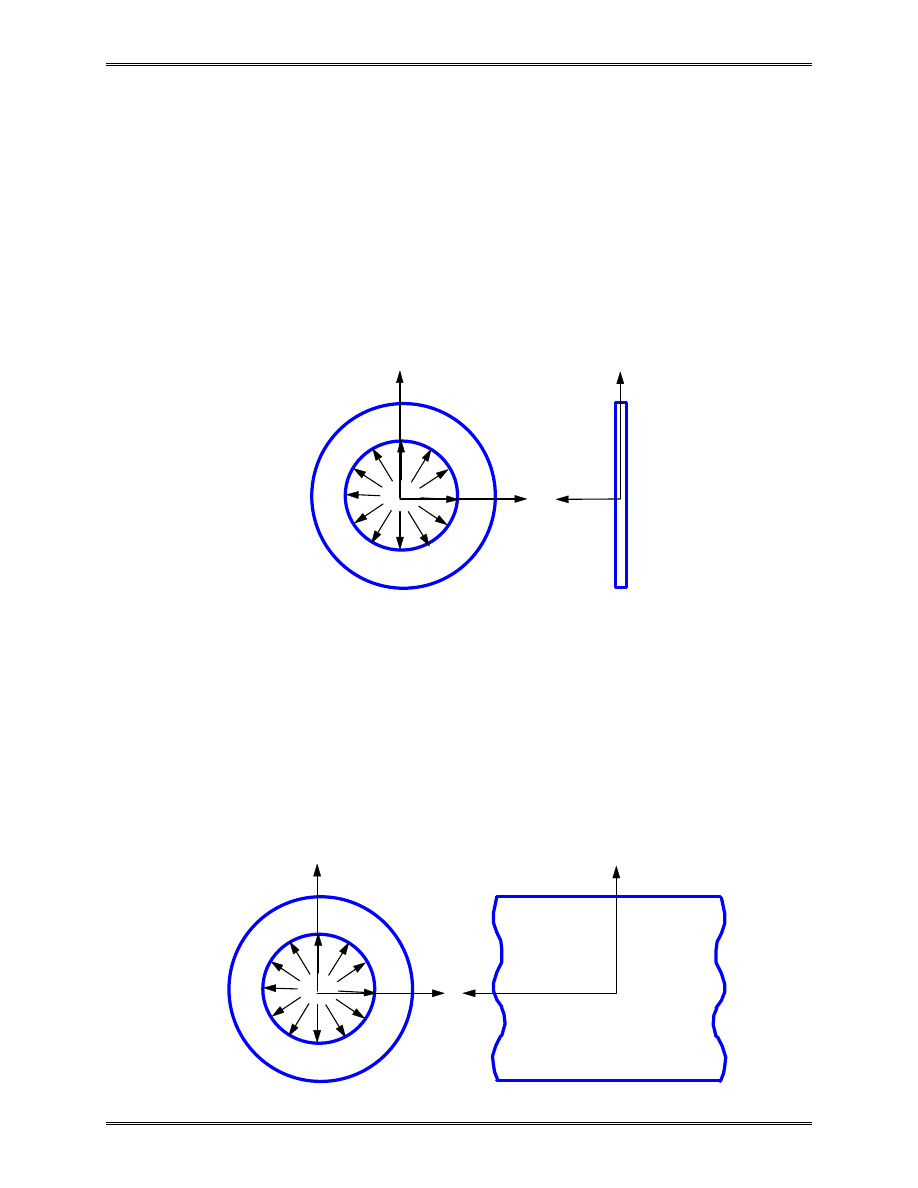
Lecture Notes: Introduction to Finite Element Method
Chapter 3. Two-Dimensional Problems
© 1998 Yijun Liu, University of Cincinnati
76
Plane (2-D) Problems
•
Plane stress:
σ τ
τ
ε
z
yz
zx
z
=
=
=
≠
0
0
(
)
(1)
A thin planar structure with constant thickness and
loading within the plane of the structure (xy-plane).
•
Plane strain:
ε γ γ
σ
z
yz
zx
z
=
=
=
≠
0
0
(
)
(2)
A long structure with a uniform cross section and
transverse loading along its length (z-direction).
p
y
x
y
z
p
y
x
y
z

Lecture Notes: Introduction to Finite Element Method
Chapter 3. Two-Dimensional Problems
© 1998 Yijun Liu, University of Cincinnati
77
Stress-Strain-Temperature (Constitutive) Relations
For elastic and isotropic materials, we have,
ε
ε
γ
ν
ν
σ
σ
τ
ε
ε
γ
x
y
xy
x
y
xy
x
y
xy
E
E
E
E
G
=
−
−
+
1
0
1
0
0
0
1
0
0
0
/
/
/
/
/
(3)
or,
ε
σ ε
=
+
−
E
1
0
where
ε
0
is the initial strain, E the Young’s modulus,
ν the
Poisson’s ratio and G the shear modulus. Note that,
G
E
=
+
2 1
(
)
ν
(4)
which means that there are only two independent materials
constants for homogeneous and isotropic materials.
We can also express stresses in terms of strains by solving
the above equation,
σ
σ
τ
ν
ν
ν
ν
ε
ε
γ
ε
ε
γ
x
y
xy
x
y
xy
x
y
xy
E
=
−
−
−
1
1
0
1
0
0
0
1
2
2
0
0
0
(
) /
(5)
or,
σ
ε σ
=
+
E
0
where
σ
ε
0
0
= −
E is the initial stress.

Lecture Notes: Introduction to Finite Element Method
Chapter 3. Two-Dimensional Problems
© 1998 Yijun Liu, University of Cincinnati
78
The above relations are valid for plane stress case. For
plane strain case, we need to replace the material constants in
the above equations in the following fashion,
E
E
G
G
→
−
→
−
→
1
1
2
ν
ν
ν
ν
(6)
For example, the stress is related to strain by
σ
σ
τ
ν
ν
ν
ν
ν
ν
ν
ε
ε
γ
ε
ε
γ
x
y
xy
x
y
xy
x
y
xy
E
=
+
−
−
−
−
−
(
)(
)
(
) /
1
1
2
1
0
1
0
0
0
1
2
2
0
0
0
in the plane strain case.
Initial strains due to temperature change (thermal loading)
is given by,
ε
ε
γ
α
α
x
y
xy
T
T
0
0
0
0
=
∆
∆
(7)
where
α
is the coefficient of thermal expansion,
∆
T the change
of temperature. Note that if the structure is free to deform under
thermal loading, there will be no (elastic) stresses in the
structure.

Lecture Notes: Introduction to Finite Element Method
Chapter 3. Two-Dimensional Problems
© 1998 Yijun Liu, University of Cincinnati
79
Strain and Displacement Relations
For small strains and small rotations, we have,
ε
∂
∂
ε
∂
∂
γ ∂
∂
∂
∂
x
y
xy
u
x
v
y
u
y
v
x
=
=
=
+
,
,
In matrix form,
ε
ε
γ
∂ ∂
∂ ∂
∂ ∂ ∂ ∂
x
y
xy
x
y
y
x
u
v
=
/
/
/
/
0
0
, or
ε
=
Du
(8)
From this relation, we know that the strains (and thus
stresses) are one order lower than the displacements, if the
displacements are represented by polynomials.
Equilibrium Equations
In elasticity theory, the stresses in the structure must satisfy
the following equilibrium equations,
∂σ
∂
∂τ
∂
∂τ
∂
∂σ
∂
x
xy
x
xy
y
y
x
y
f
x
y
f
+
+
=
+
+
=
0
0
(9)
where f
x
and f
y
are body forces (such as gravity forces) per unit
volume. In FEM, these equilibrium conditions are satisfied in
an approximate sense.
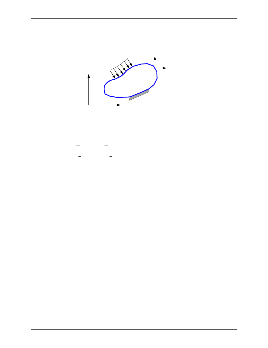
Lecture Notes: Introduction to Finite Element Method
Chapter 3. Two-Dimensional Problems
© 1998 Yijun Liu, University of Cincinnati
80
Boundary Conditions
The boundary S of the body can be divided into two parts,
S
u
and S
t
. The boundary conditions (BC’s) are described as,
u
u
v
v
S
t
t
t
t
S
u
x
x
y
y
t
=
=
=
=
,
,
,
,
on
on
(10)
in which t
x
and t
y
are traction forces (stresses on the boundary)
and the barred quantities are those with known values.
In FEM, all types of loads (distributed surface loads, body
forces, concentrated forces and moments, etc.) are converted to
point forces acting at the nodes.
Exact Elasticity Solution
The exact solution (displacements, strains and stresses) of a
given problem must satisfy the equilibrium equations (9), the
given boundary conditions (10) and compatibility conditions
(structures should deform in a continuous manner, no cracks and
overlaps in the obtained displacement fields).
x
y
p
t
x
t
y
S
u
S
t
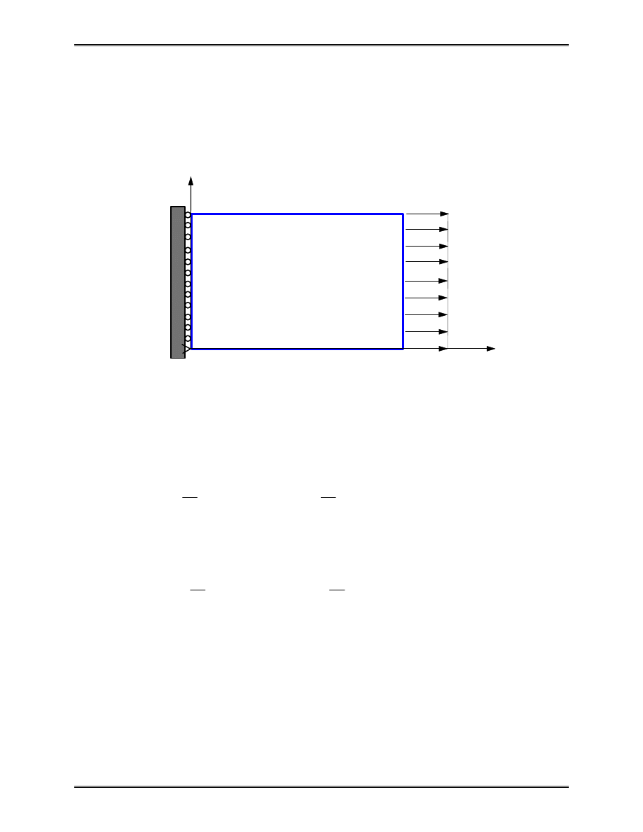
Lecture Notes: Introduction to Finite Element Method
Chapter 3. Two-Dimensional Problems
© 1998 Yijun Liu, University of Cincinnati
81
Example 3.1
A plate is supported and loaded with distributed force p as
shown in the figure. The material constants are E and
ν
.
The exact solution for this simple problem can be found
easily as follows,
Displacement:
u
p
E
x
v
p
E
y
=
= −
,
ν
Strain:
ε
ε
ν
γ
x
y
xy
p
E
p
E
=
= −
=
,
,
0
Stress:
σ
σ
τ
x
y
xy
p
=
=
=
,
,
0
0
Exact (or analytical) solutions for simple problems are
numbered (suppose there is a hole in the plate!). That is why we
need FEM!
x
y
p

Lecture Notes: Introduction to Finite Element Method
Chapter 3. Two-Dimensional Problems
© 1998 Yijun Liu, University of Cincinnati
82
II. Finite Elements for 2-D Problems
A General Formula for the Stiffness Matrix
Displacements (u, v) in a plane element are interpolated
from nodal displacements (u
i
, v
i
) using shape functions N
i
as
follows,
u
v
N
N
N
N
u
v
u
v
=
=
1
2
1
2
1
1
2
2
0
0
0
0
L
L
M
or
u
Nd
(11)
where N is the shape function matrix, u the displacement vector
and d the nodal displacement vector. Here we have assumed
that u depends on the nodal values of u only, and v on nodal
values of v only.
From strain-displacement relation (Eq.(8)), the strain vector
is,
ε
ε
=
=
=
Du
DNd
Bd
,
or
(12)
where B = DN is the strain-displacement matrix.

Lecture Notes: Introduction to Finite Element Method
Chapter 3. Two-Dimensional Problems
© 1998 Yijun Liu, University of Cincinnati
83
Consider the strain energy stored in an element,
(
)
( )
U
dV
dV
dV
dV
dV
T
V
x
x
y
y
xy
xy
V
T
V
T
V
T
T
V
T
=
=
+
+
=
=
=
=
∫
∫
∫
∫
∫
1
2
1
2
1
2
1
2
1
2
1
2
σ ε
σ ε σ ε
τ γ
ε ε
ε ε
E
E
d
B EB
d
d kd
From this, we obtain the general formula for the element
stiffness matrix,
k
B EB
=
∫
T
V
dV
(13)
Note that unlike the 1-D cases, E here is a matrix which is given
by the stress-strain relation (e.g., Eq.(5) for plane stress).
The stiffness matrix k defined by (13) is symmetric since E
is symmetric. Also note that given the material property, the
behavior of k depends on the B matrix only, which in turn on
the shape functions. Thus, the quality of finite elements in
representing the behavior of a structure is entirely determined by
the choice of shape functions.
Most commonly employed 2-D elements are linear or
quadratic triangles and quadrilaterals.
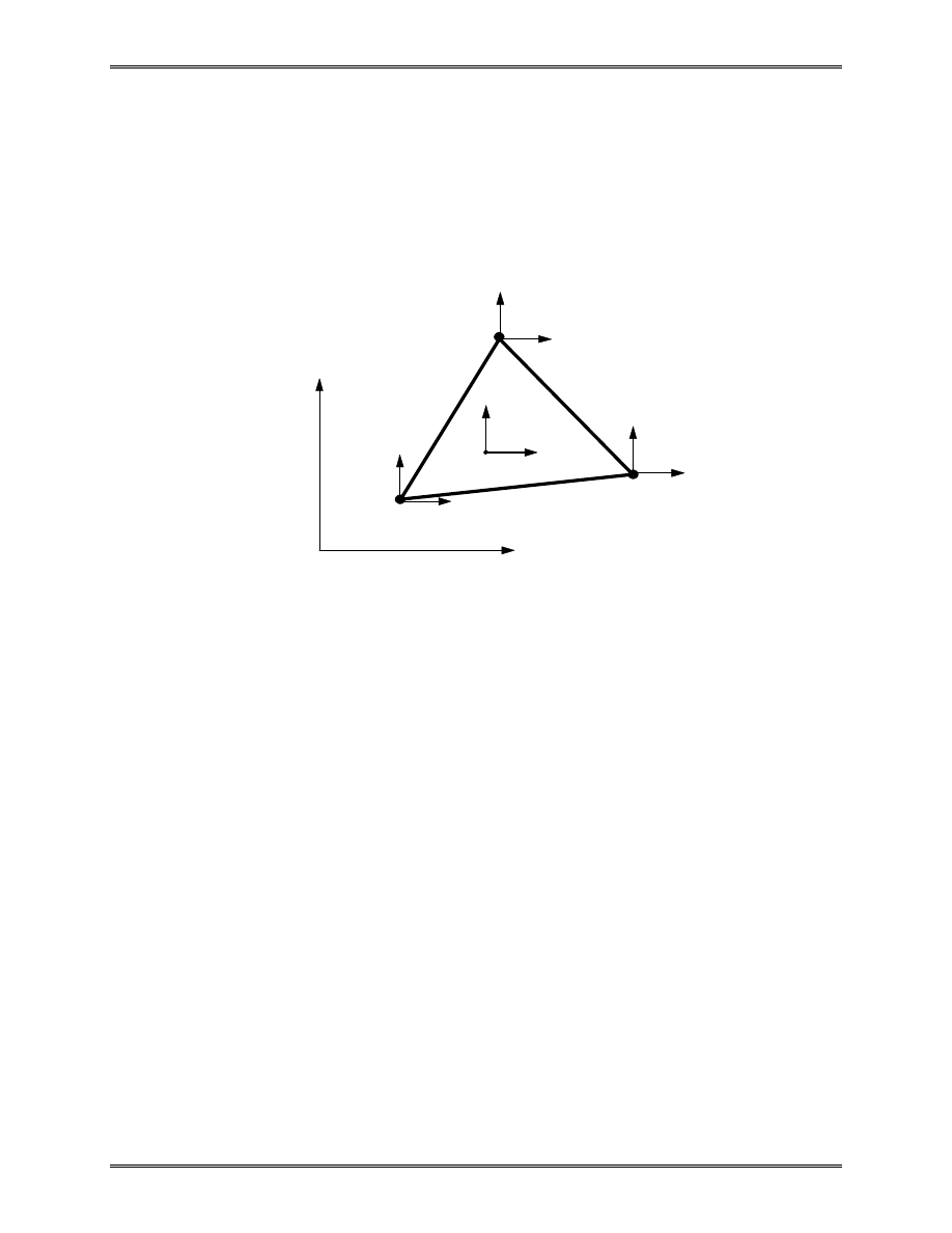
Lecture Notes: Introduction to Finite Element Method
Chapter 3. Two-Dimensional Problems
© 1998 Yijun Liu, University of Cincinnati
84
Constant Strain Triangle (CST or T3)
This is the simplest 2-D element, which is also called
linear triangular element.
For this element, we have three nodes at the vertices of the
triangle, which are numbered around the element in the
counterclockwise direction. Each node has two degrees of
freedom (can move in the x and y directions). The
displacements u and v are assumed to be linear functions within
the element, that is,
u
b
b x
b y
v
b
b x
b y
= +
+
=
+
+
1
2
3
4
5
6
,
(14)
where b
i
(i = 1, 2, ..., 6) are constants. From these, the strains
are found to be,
ε
ε
γ
x
y
xy
b
b
b
b
=
=
= +
2
6
3
5
,
,
(15)
which are constant throughout the element. Thus, we have the
name “constant strain triangle” (CST).
x
y
1
3
2
(x
1
, y
1
)
(x
3
, y
3
)
(x
2
, y
2
)
u
v
(x, y)
u
1
v
1
u
2
v
2
u
3
v
3
Linear Triangular Element

Lecture Notes: Introduction to Finite Element Method
Chapter 3. Two-Dimensional Problems
© 1998 Yijun Liu, University of Cincinnati
85
Displacements given by (14) should satisfy the following
six equations,
u
b
b x
b y
u
b
b x
b y
v
b
b x
b y
1
1
2
1
3
1
2
1
2
2
3
2
3
4
5
3
6
3
= +
+
= +
+
= +
+
M
Solving these equations, we can find the coefficients b
1
, b
2
, ...,
and b
6
in terms of nodal displacements and coordinates.
Substituting these coefficients into (14) and rearranging the
terms, we obtain,
u
v
N
N
N
N
N
N
u
v
u
v
u
v
=
1
2
3
1
2
3
1
1
2
2
3
3
0
0
0
0
0
0
(16)
where the shape functions (linear functions in x and y) are
{
}
{
}
{
}
N
A
x y
x y
y
y x
x
x
y
N
A
x y
x y
y
y x
x
x y
N
A
x y
x y
y
y x
x
x y
1
2
3
3
2
2
3
3
2
2
3
1
1
3
3
1
1
3
3
1
2
2
1
1
2
2
1
1
2
1
2
1
2
=
−
+
−
+
−
=
−
+
−
+
−
=
−
+
−
+
−
(
) (
)
(
)
(
) (
)
(
)
(
) (
)
(
)
(17)
and

Lecture Notes: Introduction to Finite Element Method
Chapter 3. Two-Dimensional Problems
© 1998 Yijun Liu, University of Cincinnati
86
A
x
y
x
y
x
y
=
1
2
1
1
1
1
1
2
2
3
3
det
(18)
is the area of the triangle (Prove this!).
Using the strain-displacement relation (8), results (16) and
(17), we have,
ε
ε
γ
x
y
xy
A
y
y
y
x
x
x
x
y
x
y
x
y
u
v
u
v
u
v
=
=
Bd
1
2
0
0
0
0
0
0
23
31
12
32
13
21
32
23
13
31
21
12
1
1
2
2
3
3
(19)
where x
ij
= x
i
- x
j
and y
ij
= y
i
- y
j
(i, j = 1, 2, 3). Again, we see
constant strains within the element. From stress-strain relation
(Eq.(5), for example), we see that stresses obtained using the
CST element are also constant.
Applying formula (13), we obtain the element stiffness
matrix for the CST element,
k
B EB
B EB
=
=
∫
T
V
T
dV
tA(
)
(20)
in which t is the thickness of the element. Notice that k for CST
is a 6 by 6 symmetric matrix. The matrix multiplication in (20)
can be carried out by a computer program.
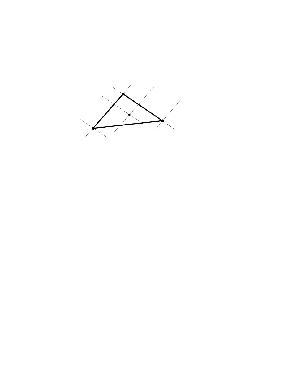
Lecture Notes: Introduction to Finite Element Method
Chapter 3. Two-Dimensional Problems
© 1998 Yijun Liu, University of Cincinnati
87
Both the expressions of the shape functions in (17) and
their derivations are lengthy and offer little insight into the
behavior of the element.
We introduce the natural coordinates
( , )
ξ η on the
triangle, then the shape functions can be represented simply by,
N
N
N
1
2
3
1
=
=
= − −
ξ
η
ξ η
,
,
(21)
Notice that,
N
N
N
1
2
3
1
+
+
=
(22)
which ensures that the rigid body translation is represented by
the chosen shape functions. Also, as in the 1-D case,
N
i
=
1
0
,
,
at node i;
at the other nodes
(23)
and varies linearly within the element. The plot for shape
function N
1
is shown in the following figure. N
2
and N
3
have
similar features.
1
3
2
ξ
=0
ξ
=1
ξ
=a
η
=0
η
=1
η
=b
The Natural Coordinates
(a, b)
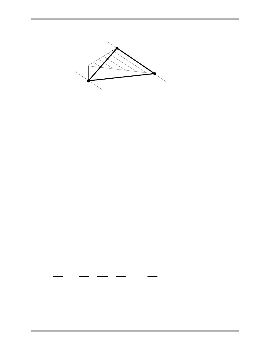
Lecture Notes: Introduction to Finite Element Method
Chapter 3. Two-Dimensional Problems
© 1998 Yijun Liu, University of Cincinnati
88
We have two coordinate systems for the element: the global
coordinates (x, y) and the natural coordinates
( , )
ξ η . The
relation between the two is given by
x
N x
N x
N x
y
N y
N y
N y
=
+
+
=
+
+
1 1
2
2
3
3
1
1
2
2
3
3
(24)
or,
x
x
x
x
y
y
y
y
=
+
+
=
+
+
13
23
3
13
23
3
ξ
η
ξ
η
(25)
where x
ij
= x
i
- x
j
and y
ij
= y
i
- y
j
(i, j = 1, 2, 3) as defined earlier.
Displacement u or v on the element can be viewed as
functions of (x, y) or
( , )
ξ η . Using the chain rule for derivatives,
we have,
∂
∂ξ
∂
∂η
∂
∂ξ
∂
∂ξ
∂
∂η
∂
∂η
∂
∂
∂
∂
∂
∂
∂
∂
u
u
x
y
x
y
u
x
u
y
u
x
u
y
=
=
J
(26)
where J is called the Jacobian matrix of the transformation.
1
3
2
ξ
=0
ξ
=1
Shape Function N
1
for CST
N
1
1

Lecture Notes: Introduction to Finite Element Method
Chapter 3. Two-Dimensional Problems
© 1998 Yijun Liu, University of Cincinnati
89
From (25), we calculate,
J
J
=
=
−
−
−
x
y
x
y
A
y
y
x
x
13
13
23
23
1
23
13
23
13
1
2
,
(27)
where
det J
=
−
=
x y
x y
A
13
23
23
13
2 has been used (A is the area of
the triangular element. Prove this!).
From (26), (27), (16) and (21) we have,
∂
∂
∂
∂
∂
∂ξ
∂
∂η
u
x
u
y
A
y
y
x
x
u
u
A
y
y
x
x
u
u
u
u
=
−
−
=
−
−
−
−
1
2
1
2
23
13
23
13
23
13
23
13
1
3
2
3
(28)
Similarly,
∂
∂
∂
∂
v
x
v
y
A
y
y
x
x
v
v
v
v
=
−
−
−
−
1
2
23
13
23
13
1
3
2
3
(29)
Using the results in (28) and (29), and the relations
ε
=
=
=
Du
DNd
Bd , we obtain the strain-displacement matrix,
B
=
1
2
0
0
0
0
0
0
23
31
12
32
13
21
32
23
13
31
21
12
A
y
y
y
x
x
x
x
y
x
y
x
y
(30)
which is the same as we derived earlier in (19).

Lecture Notes: Introduction to Finite Element Method
Chapter 3. Two-Dimensional Problems
© 1998 Yijun Liu, University of Cincinnati
90
Applications of the CST Element:
•
Use in areas where the strain gradient is small.
•
Use in mesh transition areas (fine mesh to coarse mesh).
•
Avoid using CST in stress concentration or other crucial
areas in the structure, such as edges of holes and corners.
•
Recommended for quick and preliminary FE analysis of
2-D problems.
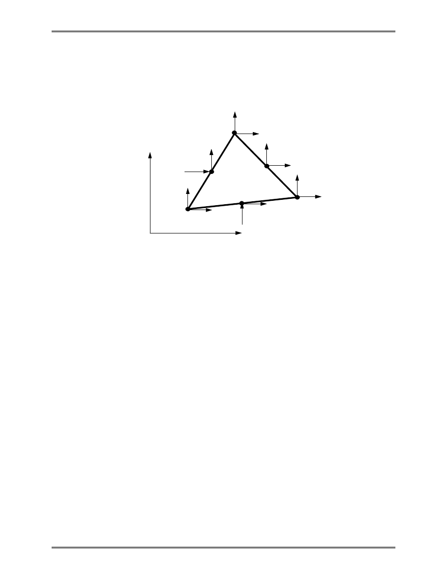
Lecture Notes: Introduction to Finite Element Method
Chapter 3. Two-Dimensional Problems
© 1998 Yijun Liu, University of Cincinnati
91
Linear Strain Triangle (LST or T6)
This element is also called quadratic triangular element.
There are six nodes on this element: three corner nodes and
three midside nodes. Each node has two degrees of freedom
(DOF) as before. The displacements (u, v) are assumed to be
quadratic functions of (x, y),
u
b
b x
b y
b x
b xy
b y
v
b
b x
b y
b x
b xy
b y
= +
+
+
+
+
= +
+
+
+
+
1
2
3
4
2
5
6
2
7
8
9
10
2
11
12
2
(31)
where b
i
(i = 1, 2, ..., 12) are constants. From these, the strains
are found to be,
ε
ε
γ
x
y
xy
b
b x
b y
b
b x
b y
b
b
b
b
x
b
b
y
= +
+
= +
+
=
+
+
+
+
+
2
4
5
9
11
12
3
8
5
10
6
11
2
2
2
2
(
) (
)
(
)
(32)
which are linear functions. Thus, we have the “linear strain
triangle” (LST), which provides better results than the CST.
x
y
1
3
2
u
1
v
1
u
2
v
2
u
3
v
3
Quadratic Triangular Element
u
4
v
4
u
5
v
5
u
6
v
6
6
5
4
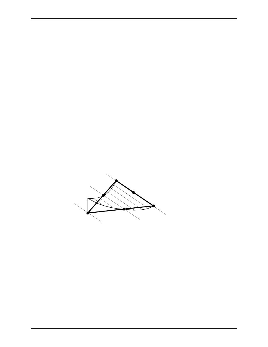
Lecture Notes: Introduction to Finite Element Method
Chapter 3. Two-Dimensional Problems
© 1998 Yijun Liu, University of Cincinnati
92
In the natural coordinate system we defined earlier, the six
shape functions for the LST element are,
N
N
N
N
N
N
1
2
3
4
5
6
2
1
2
1
2
1
4
4
4
=
−
=
−
=
−
=
=
=
ξ ξ
η η
ζ ζ
ξη
ηζ
ζ ξ
(
)
(
)
(
)
(33)
in which
ζ
ξ η
= − −
1
. Each of these six shape functions
represents a quadratic form on the element as shown in the
figure.
Displacements can be written as,
u
N u
v
N v
i
i
i
i
i
i
=
=
=
=
∑
∑
1
6
1
6
,
(34)
The element stiffness matrix is still given by
k
B EB
=
∫
T
V
dV , but here B
T
EB is quadratic in x and y. In
general, the integral has to be computed numerically.
1
3
2
ξ
=0
ξ
=1
Shape Function N
1
for LST
N
1
1
ξ
=1/2
6
5
4
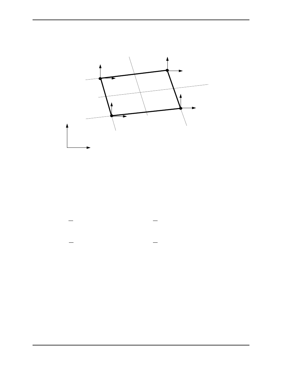
Lecture Notes: Introduction to Finite Element Method
Chapter 3. Two-Dimensional Problems
© 1998 Yijun Liu, University of Cincinnati
93
Linear Quadrilateral Element (Q4)
There are four nodes at the corners of the quadrilateral
shape. In the natural coordinate system
( , )
ξ η , the four shape
functions are,
N
N
N
N
1
2
3
4
1
4
1
1
1
4
1
1
1
4
1
1
1
4
1
1
=
−
−
=
+
−
=
+
+
=
−
+
(
)(
),
(
)(
)
(
)(
),
(
)(
)
ξ
η
ξ
η
ξ
η
ξ
η
(35)
Note that
N
i
i
=
∑
=
1
4
1 at any point inside the element, as expected.
The displacement field is given by
u
N u
v
N v
i
i
i
i
i
i
=
=
=
=
∑
∑
1
4
1
4
,
(36)
which are bilinear functions over the element.
x
y
1
3
2
u
4
v
4
u
1
v
1
u
2
v
2
u
3
v
3
Linear Quadrilateral Element
4
ξ
η
ξ
= −
1
ξ
=
1
η
= −
1
η
=
1
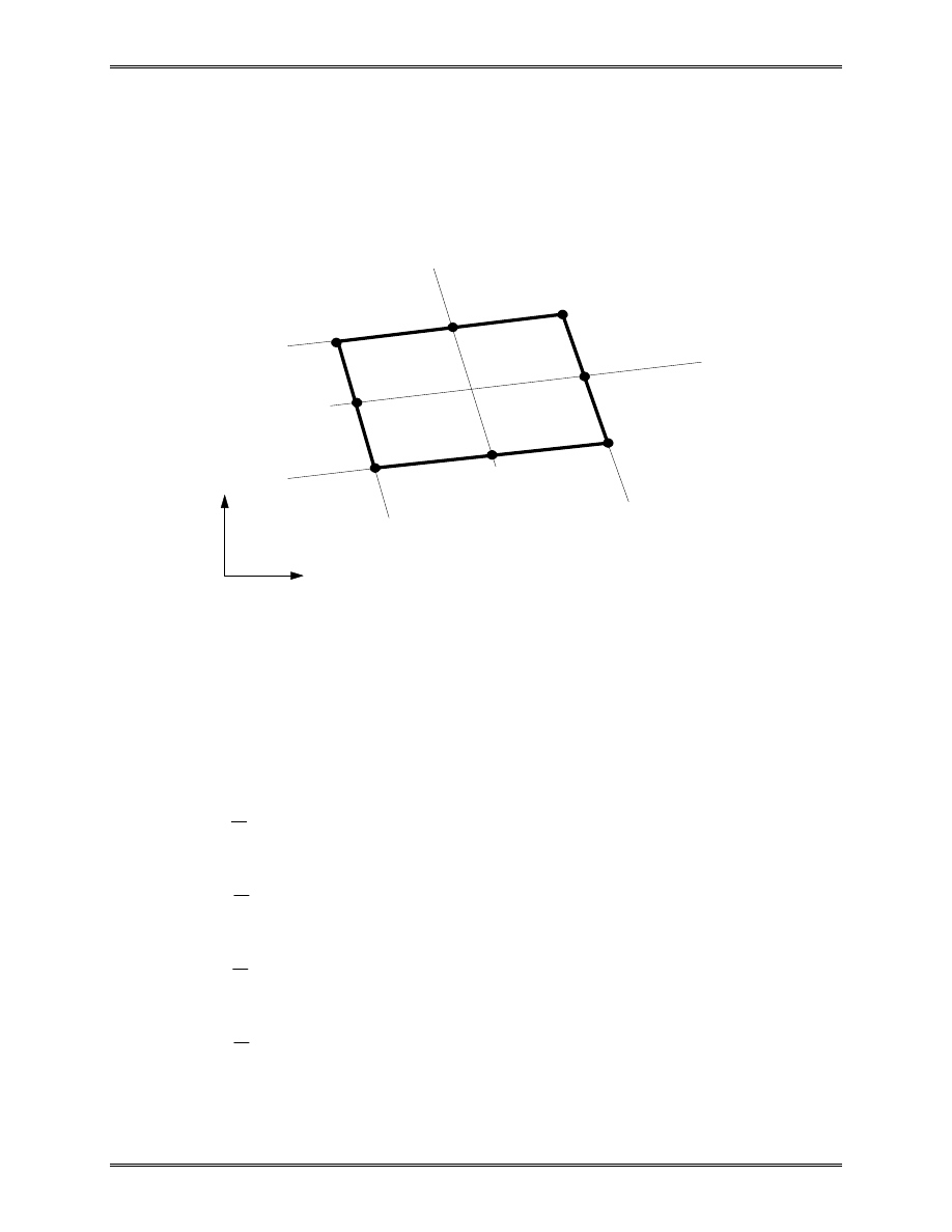
Lecture Notes: Introduction to Finite Element Method
Chapter 3. Two-Dimensional Problems
© 1998 Yijun Liu, University of Cincinnati
94
Quadratic Quadrilateral Element (Q8)
This is the most widely used element for 2-D problems due
to its high accuracy in analysis and flexibility in modeling.
There are eight nodes for this element, four corners nodes
and four midside nodes. In the natural coordinate system
( , )
ξ η ,
the eight shape functions are,
N
N
N
N
1
2
3
4
1
4
1
1
1
1
4
1
1
1
1
4
1
1
1
1
4
1
1
1
=
−
−
+ +
=
+
−
− +
=
+
+
+ −
=
−
+
− +
(
)(
)(
)
(
)(
)(
)
(
)(
)(
)
(
)(
)(
)
ξ η
ξ η
ξ η
η ξ
ξ
η ξ η
ξ
η
ξ η
(37)
x
y
1
3
2
Quadratic Quadrilateral Element
4
ξ
η
ξ
= −
1
ξ
=
1
η
= −
1
η
=
1
6
7
5
8

Lecture Notes: Introduction to Finite Element Method
Chapter 3. Two-Dimensional Problems
© 1998 Yijun Liu, University of Cincinnati
95
N
N
N
N
5
2
6
2
7
2
8
2
1
2
1
1
1
2
1
1
1
2
1
1
1
2
1
1
=
−
−
=
+
−
=
+
−
=
−
−
(
)(
)
(
)(
)
(
)(
)
(
)(
)
η
ξ
ξ
η
η
ξ
ξ
η
Again, we have
N
i
i
=
∑
=
1
8
1 at any point inside the element.
The displacement field is given by
u
N u
v
N v
i
i
i
i
i
i
=
=
=
=
∑
∑
1
8
1
8
,
(38)
which are quadratic functions over the element. Strains and
stresses over a quadratic quadrilateral element are linear
functions, which are better representations.
Notes:
•
Q4 and T3 are usually used together in a mesh with
linear elements.
•
Q8 and T6 are usually applied in a mesh composed of
quadratic elements.
•
Quadratic elements are preferred for stress analysis,
because of their high accuracy and the flexibility in
modeling complex geometry, such as curved boundaries.
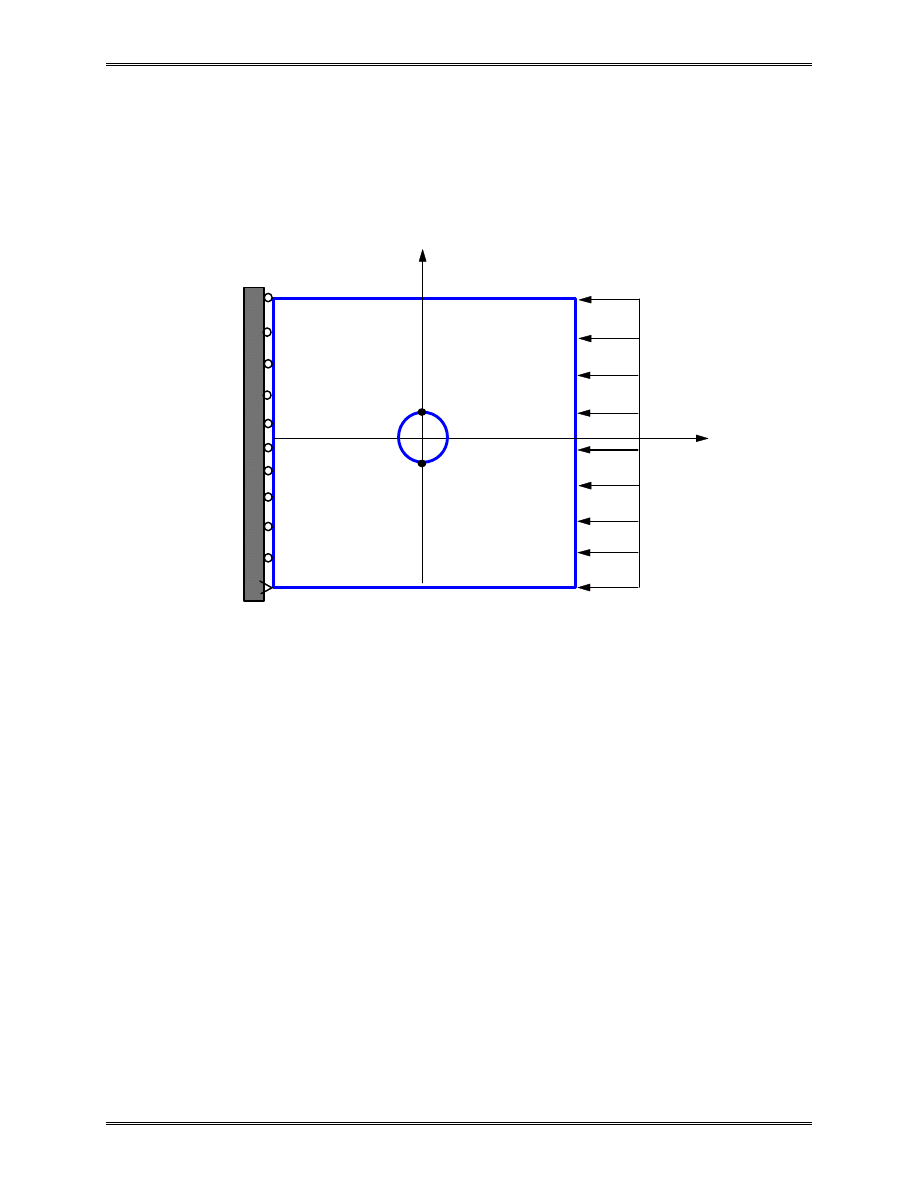
Lecture Notes: Introduction to Finite Element Method
Chapter 3. Two-Dimensional Problems
© 1998 Yijun Liu, University of Cincinnati
96
Example 3.2
A square plate with a hole at the center and under pressure
in one direction.
The dimension of the plate is 10 in. x 10 in., thickness is
0.1 in. and radius of the hole is 1 in. Assume E = 10x10
6
psi, v
= 0.3 and p = 100 psi. Find the maximum stress in the plate.
FE Analysis:
From the knowledge of stress concentrations, we should
expect the maximum stresses occur at points A and B on the
edge of the hole. Value of this stress should be around 3p (=
300 psi) which is the exact solution for an infinitely large plate
with a hole.
x
y
p
B
A
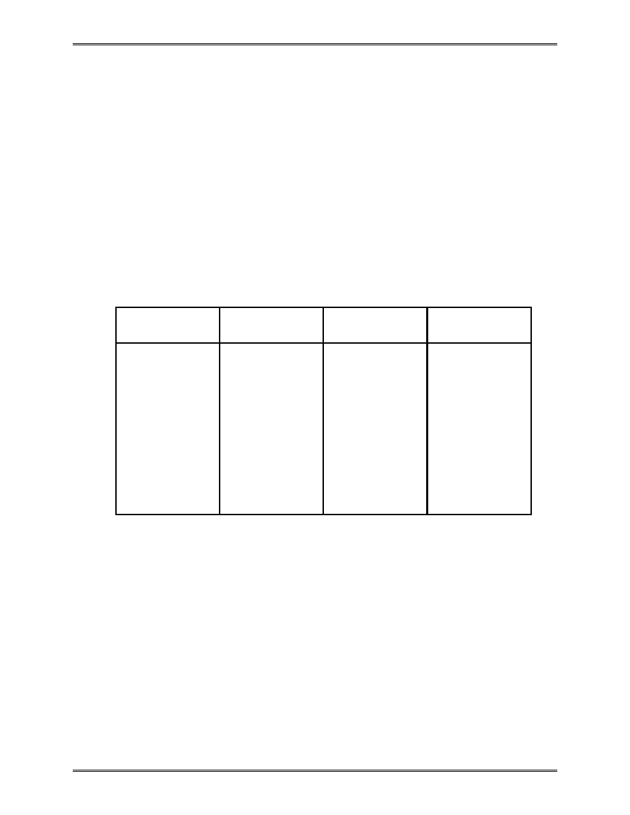
Lecture Notes: Introduction to Finite Element Method
Chapter 3. Two-Dimensional Problems
© 1998 Yijun Liu, University of Cincinnati
97
We use the ANSYS FEA software to do the modeling
(meshing) and analysis, using quadratic triangular (T6 or LST),
linear quadrilateral (Q4) and quadratic quadrilateral (Q8)
elements. Linear triangles (CST or T3) is NOT available in
ANSYS.
The stress calculations are listed in the following table,
along with the number of elements and DOF used, for
comparison.
Table. FEA Stress Results
Elem. Type
No. Elem.
DOF
Max.
σ
(psi)
T6
966
4056
310.1
Q4
493
1082
286.0
Q8
493
3150
327.1
...
...
...
...
Q8
2727
16,826
322.3
Discussions:
•
Check the deformed shape of the plate
•
Check convergence (use a finer mesh, if possible)
•
Less elements (~ 100) should be enough to achieve the
same accuracy with a better or “smarter” mesh
•
We’ll redo this example in next chapter employing the
symmetry conditions.
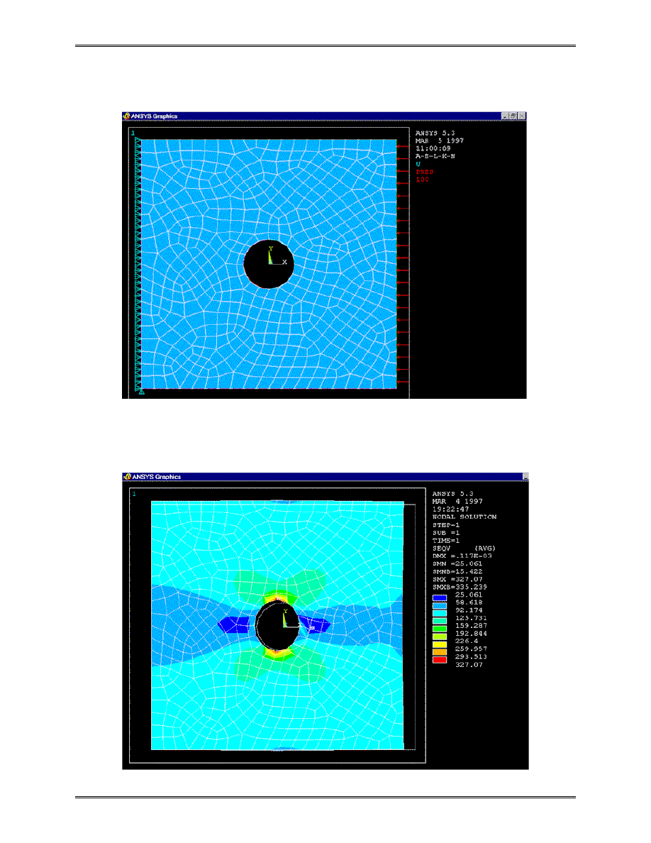
Lecture Notes: Introduction to Finite Element Method
Chapter 3. Two-Dimensional Problems
© 1998 Yijun Liu, University of Cincinnati
98
FEA Mesh (Q8, 493 elements)
FEA Stress Plot (Q8, 493 elements)
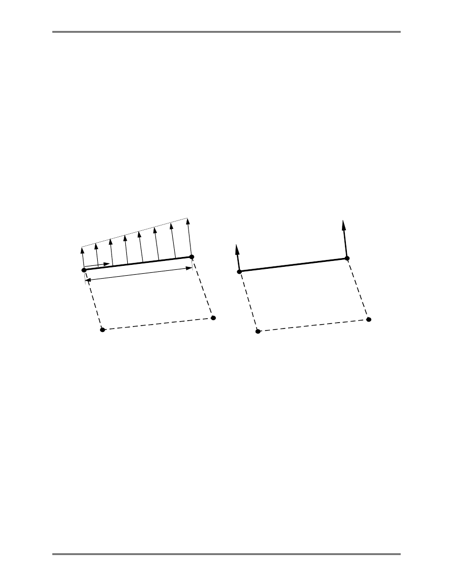
Lecture Notes: Introduction to Finite Element Method
Chapter 3. Two-Dimensional Problems
© 1998 Yijun Liu, University of Cincinnati
99
Transformation of Loads
Concentrated load (point forces), surface traction (pressure
loads) and body force (weight) are the main types of loads
applied to a structure. Both traction and body forces need to be
converted to nodal forces in the FEA, since they cannot be
applied to the FE model directly. The conversions of these
loads are based on the same idea (the equivalent-work concept)
which we have used for the cases of bar and beam elements.
Suppose, for example, we have a linearly varying traction q
on a Q4 element edge, as shown in the figure. The traction is
normal to the boundary. Using the local (tangential) coordinate
s, we can write the work done by the traction q as,
W
t u s q s ds
q
n
L
=
∫
( ) ( )
0
where t is the thickness, L the side length and u
n
the component
of displacement normal to the edge AB.
Traction on a Q4 element
A
B
L
s
q
q
A
q
B
A
B
f
A
f
B

Lecture Notes: Introduction to Finite Element Method
Chapter 3. Two-Dimensional Problems
© 1998 Yijun Liu, University of Cincinnati
100
For the Q4 element (linear displacement field), we have
u s
s L u
s L u
n
nA
nB
( )
(
/ )
( / )
= −
+
1
The traction q(s), which is also linear, is given in a similar way,
q s
s L q
s L q
A
B
( )
(
/ )
( / )
= −
+
1
Thus, we have,
[
]
[
]
[
]
[
]
W
t
u
u
s L
s L
s L
s L
q
q
ds
u
u
t
s L
s L
s L
s L
s L
s L
ds
q
q
u
u
tL
q
q
q
nA
nB
A
B
L
nA
nB
L
A
B
nA
nB
A
B
=
−
−
=
−
−
−
=
∫
∫
1
1
1
1
1
6
2
1
1
2
0
2
2
0
/
/
/
/
(
/ )
( / )(
/ )
( / )(
/ )
( / )
and the equivalent nodal force vector is,
f
f
tL
q
q
A
B
A
B
=
6
2
1
1
2
Note, for constant q, we have,
f
f
qtL
A
B
=
2
1
1
For quadratic elements (either triangular or quadrilateral),
the traction is converted to forces at three nodes along the edge,
instead of two nodes.
Traction tangent to the boundary, as well as body forces,
are converted to nodal forces in a similar way.

Lecture Notes: Introduction to Finite Element Method
Chapter 3. Two-Dimensional Problems
© 1998 Yijun Liu, University of Cincinnati
101
Stress Calculation
The stress in an element is determined by the following
relation,
σ
σ
τ
ε
ε
γ
x
y
xy
x
y
xy
=
=
E
EBd
(39)
where B is the strain-nodal displacement matrix and d is the
nodal displacement vector which is known for each element
once the global FE equation has been solved.
Stresses can be evaluated at any point inside the element
(such as the center) or at the nodes. Contour plots are usually
used in FEA software packages (during post-process) for users
to visually inspect the stress results.
The von Mises Stress:
The von Mises stress is the effective or equivalent stress for
2-D and 3-D stress analysis. For a ductile material, the stress
level is considered to be safe, if
σ
σ
e
Y
≤
where
σ
e
is the von Mises stress and
σ
Y
the yield stress of the
material. This is a generalization of the 1-D (experimental)
result to 2-D and 3-D situations.
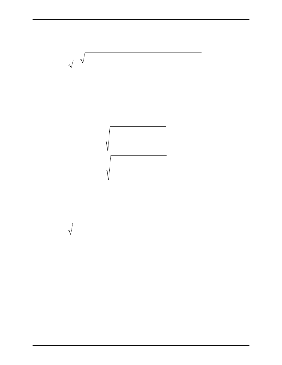
Lecture Notes: Introduction to Finite Element Method
Chapter 3. Two-Dimensional Problems
© 1998 Yijun Liu, University of Cincinnati
102
The von Mises stress is defined by
σ
σ σ
σ σ
σ σ
e
=
−
+
−
+
−
1
2
1
2
2
2
3
2
3
1
2
(
)
(
)
(
)
(40)
in which
σ σ
σ
1
2
3
,
and
are the three principle stresses at the
considered point in a structure.
For 2-D problems, the two principle stresses in the plane
are determined by
σ
σ σ
σ σ
τ
σ
σ σ
σ σ
τ
1
2
2
2
2
2
2
2
2
2
P
x
y
x
y
xy
P
x
y
x
y
xy
=
+
+
−
+
=
+
−
−
+
(41)
Thus, we can also express the von Mises stress in terms of
the stress components in the xy coordinate system. For plane
stress conditions, we have,
σ
σ σ
σ σ
τ
e
x
y
x
y
xy
=
+
−
−
(
)
(
)
2
2
3
(42)
Averaged Stresses:
Stresses are usually averaged at nodes in FEA software
packages to provide more accurate stress values. This option
should be turned off at nodes between two materials or other
geometry discontinuity locations where stress discontinuity does
exist.
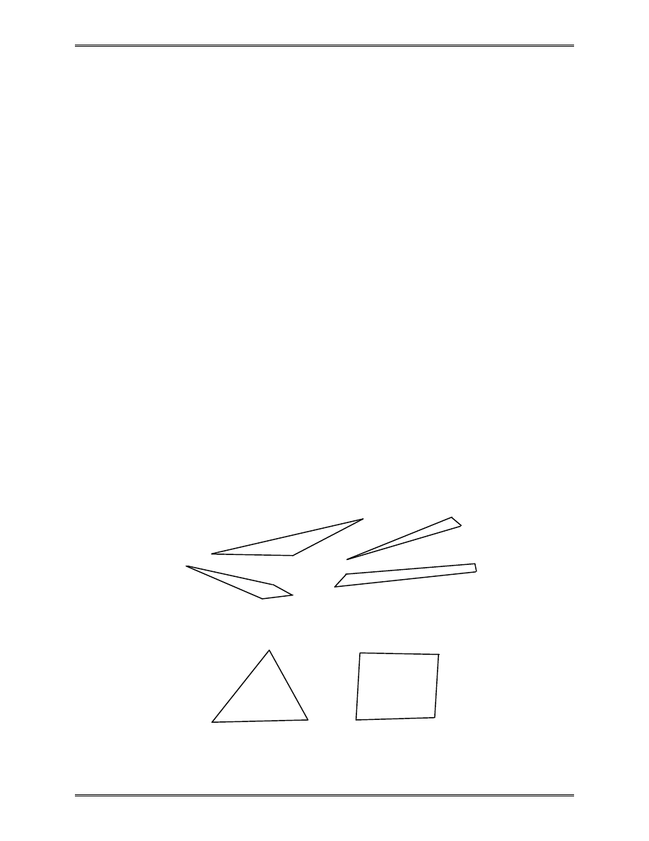
Lecture Notes: Introduction to Finite Element Method
Chapter 3. Two-Dimensional Problems
© 1998 Yijun Liu, University of Cincinnati
103
Discussions
1) Know the behaviors of each type of elements:
T3 and Q4: linear displacement, constant strain and stress;
T6 and Q8: quadratic displacement, linear strain and stress.
2) Choose the right type of elements for a given problem:
When in doubt, use higher order elements or a finer mesh.
3) Avoid elements with large aspect ratios and corner angles:
Aspect ratio = L
max
/ L
min
where L
max
and L
min
are the largest and smallest characteristic
lengths of an element, respectively.
Elements with Bad Shapes
Elements with Nice Shapes
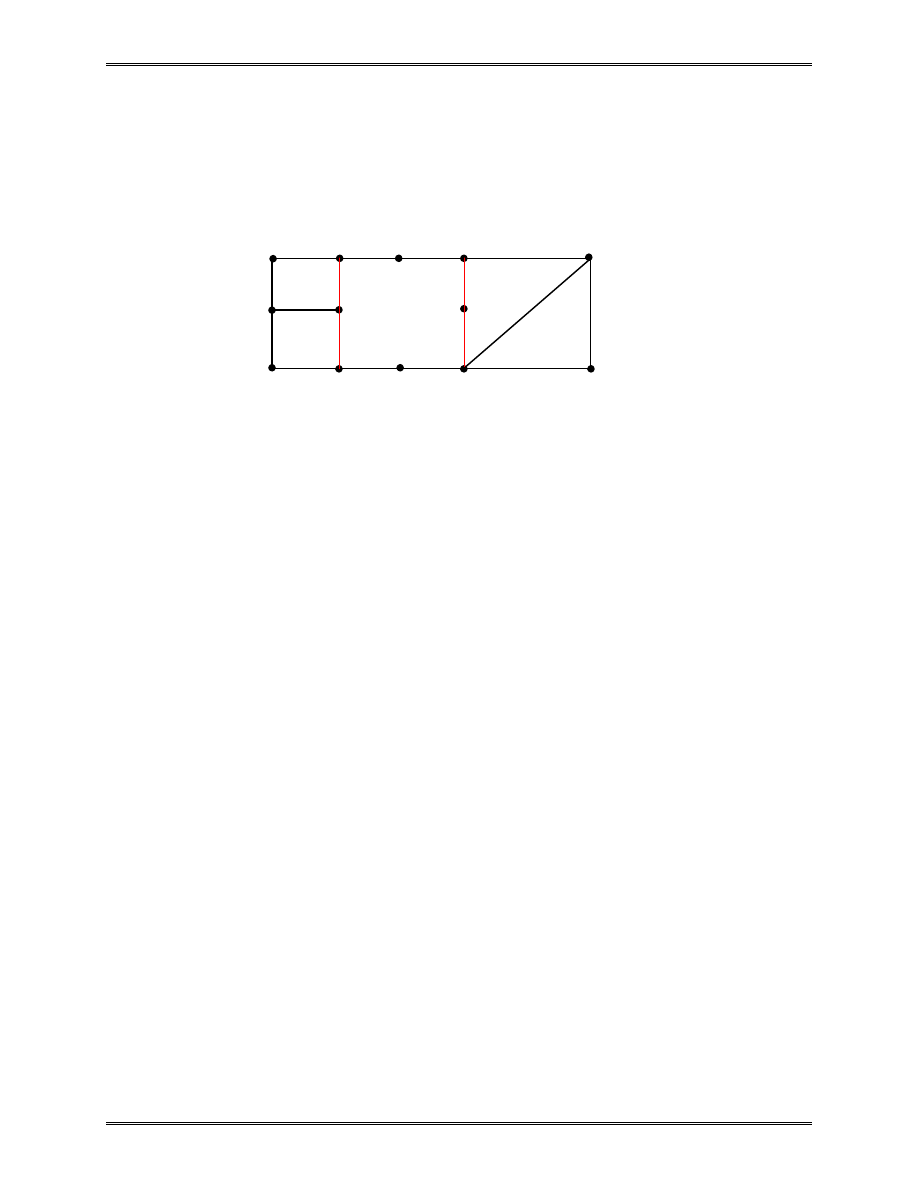
Lecture Notes: Introduction to Finite Element Method
Chapter 3. Two-Dimensional Problems
© 1998 Yijun Liu, University of Cincinnati
104
4) Connect the elements properly:
Don’t leave unintended gaps or free elements in FE models.
Readings:
Sections 3.1-3.5 and 3.8-3.12 of Cook’s book.
A
B
C
D
Improper connections (gaps along AB and CD)

Lecture Notes: Introduction to Finite Element Method
Chapter 4. FE Modeling and Solution Techniques
© 1998 Yijun Liu, University of Cincinnati
105
Chapter 4. Finite Element Modeling and
Solution Techniques
I. Symmetry
A structure possesses symmetry if its components are
arranged in a periodic or reflective manner.
Types of Symmetry:
•
Reflective (mirror, bilateral) symmetry
•
Rotational (cyclic) symmetry
•
Axisymmetry
•
Translational symmetry
•
...
Examples:
…

Lecture Notes: Introduction to Finite Element Method
Chapter 4. FE Modeling and Solution Techniques
© 1998 Yijun Liu, University of Cincinnati
106
Applications of the symmetry properties:
•
Reducing the size of the problems (save CPU time, disk
space, postprocessing effort, etc.)
•
Simplifying the modeling task
•
Checking the FEA results
•
...
Symmetry of a structure should be fully exploited and
retained in the FE model to ensure the efficiency and quality of
FE solutions.
Examples:
…
Cautions:
In vibration and buckling analyses, symmetry concepts, in
general, should not be used in FE solutions (works fine in
modeling), since symmetric structures often have antisymmetric
vibration or buckling modes.
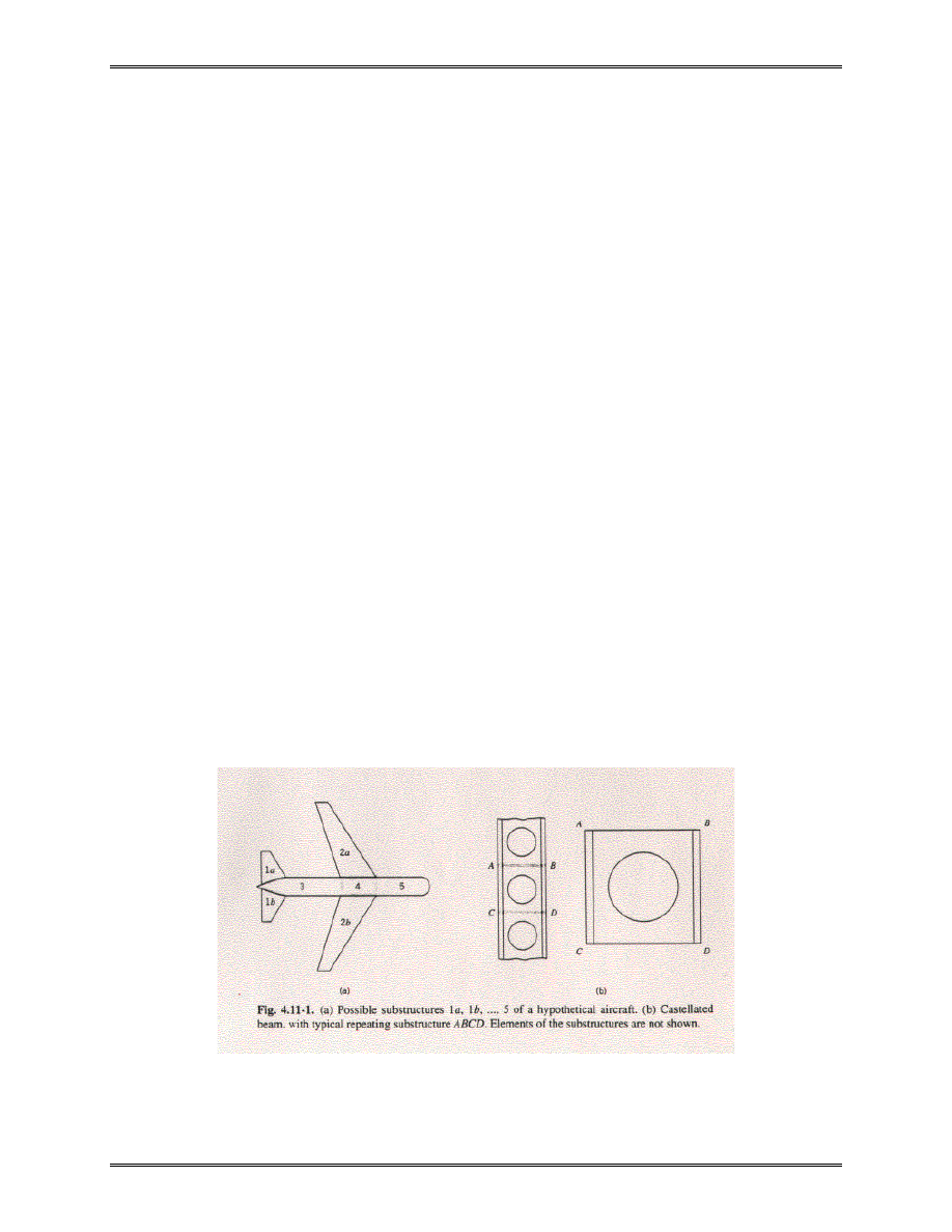
Lecture Notes: Introduction to Finite Element Method
Chapter 4. FE Modeling and Solution Techniques
© 1998 Yijun Liu, University of Cincinnati
107
II. Substructures (Superelements)
Substructuring is a process of analyzing a large structure as
a collection of (natural) components. The FE models for these
components are called substructures or superelements (SE).
Physical Meaning:
A finite element model of a portion of structure.
Mathematical Meaning:
Boundary matrices which are load and stiffness matrices
reduced (condensed) from the interior points to the exterior or
boundary points.

Lecture Notes: Introduction to Finite Element Method
Chapter 4. FE Modeling and Solution Techniques
© 1998 Yijun Liu, University of Cincinnati
108
Advantages of Using Substructures/Superelements:
•
Large problems (which will otherwise exceed your
computer capabilities)
•
Less CPU time per run once the superelements have
been processed (i.e., matrices have been saved)
•
Components may be modeled by different groups
•
Partial redesign requires only partial reanalysis (reduced
cost)
•
Efficient for problems with local nonlinearities (such as
confined plastic deformations) which can be placed in
one superelement (residual structure)
•
Exact for static stress analysis
Disadvantages:
•
Increased overhead for file management
•
Matrix condensation for dynamic problems introduce
new approximations
•
...

Lecture Notes: Introduction to Finite Element Method
Chapter 4. FE Modeling and Solution Techniques
© 1998 Yijun Liu, University of Cincinnati
109
III.
Equation Solving
Direct Methods (Gauss Elimination):
•
Solution time proportional to NB
2
(N is the dimension of
the matrix, B the bandwidth)
•
Suitable for small to medium problems, or slender
structures (small bandwidth)
•
Easy to handle multiple load cases
Iterative Methods:
•
Solution time is unknown beforehand
•
Reduced storage requirement
•
Suitable for large problems, or bulky structures (large
bandwidth, converge faster)
•
Need solving again for different load cases

Lecture Notes: Introduction to Finite Element Method
Chapter 4. FE Modeling and Solution Techniques
© 1998 Yijun Liu, University of Cincinnati
110
Gauss Elimination - Example:
−
=
−
−
−
−
3
1
2
3
3
0
3
4
2
0
2
8
3
2
1
x
x
x
or
b
Ax
=
.
Forward Elimination:
Form
−
−
−
−
−
3
1
2
3
3
0
3
4
2
0
2
8
)
3
(
)
2
(
)
1
(
;
(1) + 4 x (2)
⇒
(2):
−
−
−
−
3
2
2
3
3
0
12
14
0
0
2
8
)
3
(
)
2
(
)
1
(
;
(2) +
3
14
(3)
⇒
(3):
−
−
−
12
2
2
2
0
0
12
14
0
0
2
8
)
3
(
)
2
(
)
1
(
;
Back Substitution:
5
.
1
8
/
)
2
2
(
5
14
/
)
12
2
(
6
2
/
12
2
1
3
2
3
=
+
=
=
+
−
=
=
=
x
x
x
x
x
or
=
6
5
5
1.
x
.

Lecture Notes: Introduction to Finite Element Method
Chapter 4. FE Modeling and Solution Techniques
© 1998 Yijun Liu, University of Cincinnati
111
Iterative Method - Example:
The Gauss-Seidel Method
b
Ax
=
(A is symmetric)
or
.
...,
,
2
,
1
,
1
N
i
b
x
a
N
j
i
j
ij
=
=
∑
=
Start with an estimate
)
( 0
x
and then iterate using the following:
.
...,
,
2
,
1
for
,
1
1
1
1
)
(
)
1
(
)
1
(
N
i
x
a
x
a
b
a
x
i
j
N
i
j
k
j
ij
k
j
ij
i
ii
k
i
=
−
−
=
∑
∑
−
=
+
=
+
+
In vector form,
[
]
,
)
(
)
1
(
1
)
1
(
k
T
L
k
L
D
k
x
A
x
A
b
A
x
−
−
=
+
−
+
where
〉
〈
=
ii
D
a
A
is the diagonal matrix of A,
L
A
is the lower triangular matrix of A,
such that
.
T
L
L
D
A
A
A
A
+
+
=
Iterations continue until solution x converges, i.e.
,
)
(
)
(
)
1
(
ε
≤
−
+
k
k
k
x
x
x
where
ε
is the tolerance for convergence control.
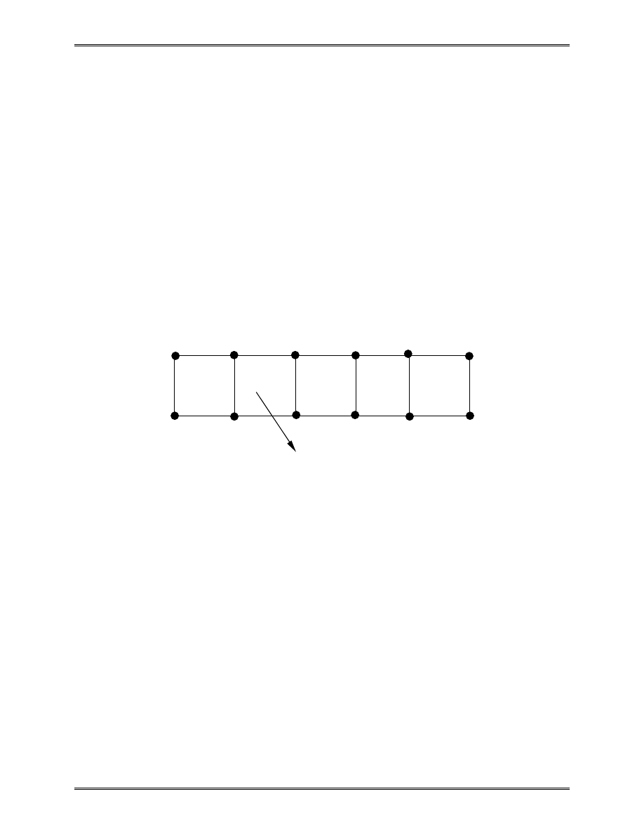
Lecture Notes: Introduction to Finite Element Method
Chapter 4. FE Modeling and Solution Techniques
© 1998 Yijun Liu, University of Cincinnati
112
IV. Nature of Finite Element Solutions
•
FE Model – A mathematical model of the real structure,
based on many approximations.
•
Real Structure -- Infinite number of nodes (physical
points or particles), thus infinite number of DOF’s.
•
FE Model – finite number of nodes, thus finite number
of DOF’s.
ð Displacement field is controlled (or constrained) by the
values at a limited number of nodes.
Stiffening Effect:
•
FE Model is stiffer than the real structure.
•
In general, displacement results are smaller in
magnitudes than the exact values.
∑
=
=
4
1
:
element
an
on
that
Recall
α
α
α
u
N
u
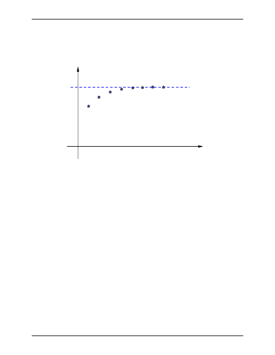
Lecture Notes: Introduction to Finite Element Method
Chapter 4. FE Modeling and Solution Techniques
© 1998 Yijun Liu, University of Cincinnati
113
Hence, FEM solution of displacement provides a lower
bound of the exact solution.
The FEM solution approaches the exact solution from
below.
This is true for displacement based FEA only!
No. of DOF’s
∆
(Displacement)
Exact Solution
FEM Solutions
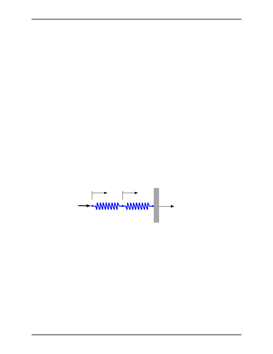
Lecture Notes: Introduction to Finite Element Method
Chapter 4. FE Modeling and Solution Techniques
© 1998 Yijun Liu, University of Cincinnati
114
V. Numerical Error
Error
≠
Mistakes in FEM (modeling or solution).
Types of Error:
•
Modeling Error (beam, plate … theories)
•
Discretization Error (finite, piecewise … )
•
Numerical Error ( in solving FE equations)
Example (numerical error):
FE Equations:
=
+
−
−
0
2
1
2
1
1
1
1
P
u
u
k
k
k
k
k
and
2
1
k
k
Det
=
K
.
The system will be singular if k
2
is small compared with k
1
.
k
1
x
k
2
1
2
P
u
1
u
2
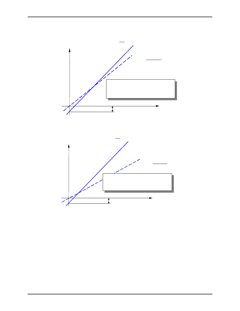
Lecture Notes: Introduction to Finite Element Method
Chapter 4. FE Modeling and Solution Techniques
© 1998 Yijun Liu, University of Cincinnati
115
•
Large difference in stiffness of different parts in FE
model may cause ill-conditioning in FE equations.
Hence giving results with large errors.
•
Ill-conditioned system of equations can lead to large
changes in solution with small changes in input
(right hand side vector).
1
u
2
u
1
2
1
1
2
u
k
k
k
u
+
=
1
1
2
k
P
u
u
−
=
k
2
<< k
1
(two lines close):
ð System ill-conditioned.
P/k
1
1
u
2
u
1
2
1
1
2
u
k
k
k
u
+
=
1
1
2
k
P
u
u
−
=
k
2
>> k
1
(two line apart):
ð System well conditioned.
P/k
1

Lecture Notes: Introduction to Finite Element Method
Chapter 4. FE Modeling and Solution Techniques
© 1998 Yijun Liu, University of Cincinnati
116
VI. Convergence of FE Solutions
As the mesh in an FE model is “refined” repeatedly, the FE
solution will converge to the exact solution of the mathematical
model of the problem (the model based on bar, beam, plane
stress/strain, plate, shell, or 3-D elasticity theories or
assumptions).
Types of Refinement:
h-refinement:
reduce the size of the element (“h” refers to the
typical size of the elements);
p-refinement:
Increase the order of the polynomials on an
element (linear to quadratic, etc.; “h” refers to
the highest order in a polynomial);
r-refinement:
re-arrange the nodes in the mesh;
hp-refinement: Combination of the h- and p-refinements
(better results!).
Examples:
…

Lecture Notes: Introduction to Finite Element Method
Chapter 4. FE Modeling and Solution Techniques
© 1998 Yijun Liu, University of Cincinnati
117
VII. Adaptivity (h-, p-, and hp-Methods)
•
Future of FE applications
•
Automatic refinement of FE meshes until converged
results are obtained
•
User’s responsibility reduced: only need to generate a
good initial mesh
Error Indicators:
Define,
σ --- element by element stress field (discontinuous),
σ
*
--- averaged or smooth stress (continuous),
σ
E
=
σ
-
σ
*
--- the error stress field.
Compute strain energy,
∫
∑
−
=
=
=
i
V
T
i
M
i
i
dV
U
U
U
s
E
s
1
1
2
1
,
;
∫
∑
−
=
=
=
i
i
V
T
M
i
i
dV
U
U
U
*
1
*
*
1
*
*
2
1
,
s
E
s
;
∫
∑
−
=
=
=
i
V
E
T
E
i
E
M
i
i
E
E
dV
U
U
U
s
E
s
1
1
2
1
,
;
where M is the total number of elements,
i
V is the volume of the
element i.

Lecture Notes: Introduction to Finite Element Method
Chapter 4. FE Modeling and Solution Techniques
© 1998 Yijun Liu, University of Cincinnati
118
One error indicator --- the relative energy error:
)
1
0
(
.
2
/
1
≤
≤
+
=
η
η
E
E
U
U
U
The indicator
η
is computed after each FE solution. Refinement
of the FE model continues until, say
η
≤
0.05.
=> converged FE solution.
Examples:
…

Lecture Notes: Introduction to Finite Element Method Chapter 5. Plate and Shell Elements
© 1999 Yijun Liu, University of Cincinnati
119
Chapter 5. Plate and Shell Elements
I. Plate Theory
•
Flat plate
•
Lateral loading
•
Bending behavior dominates
Note the following similarity:
1-D straight beam model
ó 2-D flat plate model
Applications:
•
Shear walls
•
Floor panels
•
Shelves
•
…
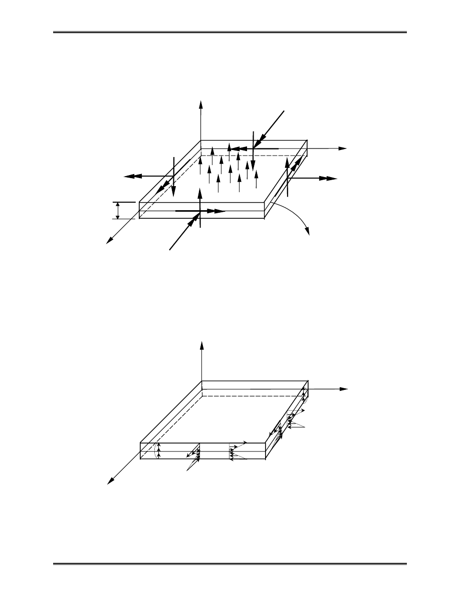
Lecture Notes: Introduction to Finite Element Method Chapter 5. Plate and Shell Elements
© 1999 Yijun Liu, University of Cincinnati
120
Forces and Moments Acting on the Plate:
Stresses:
M
xy
M
x
Q
x
M
xy
M
y
Q
y
x
y
z
Mid surface
q(x,y)
t
∆
x
∆
y
σ
x
τ
xz
x
y
z
τ
xy
σ
y
τ
xy
τ
yz

Lecture Notes: Introduction to Finite Element Method Chapter 5. Plate and Shell Elements
© 1999 Yijun Liu, University of Cincinnati
121
Relations Between Forces and Stresses
Bending moments (per unit length):
)
/
(
,
2
/
2
/
m
m
N
zdz
M
t
t
x
x
⋅
=
∫
−
σ
(1)
)
/
(
,
2
/
2
/
m
m
N
zdz
M
t
t
y
y
⋅
=
∫
−
σ
(2)
Twisting moment (per unit length):
)
/
(
,
2
/
2
/
m
m
N
zdz
M
t
t
xy
xy
⋅
=
∫
−
τ
(3)
Shear Forces (per unit length):
)
/
(
,
2
/
2
/
m
N
dz
Q
t
t
xz
x
∫
−
=
τ
(4)
)
/
(
,
2
/
2
/
m
N
dz
Q
t
t
yz
y
∫
−
=
τ
(5)
Maximum bending stresses:
2
max
2
max
6
)
(
,
6
)
(
t
M
t
M
y
y
x
x
±
=
±
=
σ
σ
.
(6)
•
Maximum stress is always at
2
/
t
z
±
=
•
No bending stresses at midsurface (similar to the beam
model)
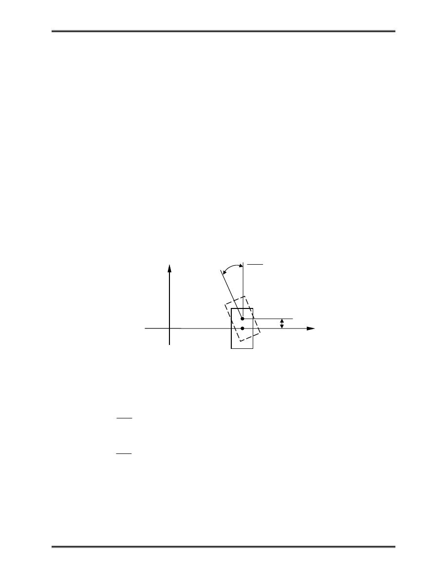
Lecture Notes: Introduction to Finite Element Method Chapter 5. Plate and Shell Elements
© 1999 Yijun Liu, University of Cincinnati
122
Thin Plate Theory ( Kirchhoff Plate Theory)
Assumptions (similar to those in the beam theory):
A straight line along the normal to the mid surface remains
straight and normal to the deflected mid surface after loading,
that is, these is no transverse shear deformation:
0
=
=
yz
xz
γ
γ
.
Displacement:
.
,
)
(
),
,
(
y
w
z
v
x
w
z
u
deflection
y
x
w
w
∂
∂
∂
∂
−
=
−
=
=
(7)
x
z
w
x
w
∂
∂

Lecture Notes: Introduction to Finite Element Method Chapter 5. Plate and Shell Elements
© 1999 Yijun Liu, University of Cincinnati
123
Strains:
.
2
,
,
2
2
2
2
2
y
x
w
z
y
w
z
x
w
z
xy
y
x
∂
∂
∂
γ
∂
∂
ε
∂
∂
ε
−
=
−
=
−
=
(8)
Note that there is no stretch of the mid surface due to the
deflection (bending) of the plate.
Stresses (plane stress state):
−
−
=
xy
y
x
xy
y
x
E
γ
ε
ε
ν
ν
ν
ν
τ
σ
σ
2
/
)
1
(
0
0
0
1
0
1
1
2
,
or,
∂
∂
∂
∂
∂
∂
∂
−
−
−
=
y
x
w
y
w
x
w
E
z
xy
y
x
2
2
2
2
2
2
)
1
(
0
0
0
1
0
1
1
ν
ν
ν
ν
τ
σ
σ
.
(9)
Main variable: deflection
)
,
(
y
x
w
w
=
.

Lecture Notes: Introduction to Finite Element Method Chapter 5. Plate and Shell Elements
© 1999 Yijun Liu, University of Cincinnati
124
Governing Equation:
)
,
(
4
y
x
q
w
D
=
∇
, (10)
where
),
2
(
4
4
2
2
4
4
4
4
y
y
x
x
∂
∂
∂
∂
∂
∂
∂
+
+
≡
∇
)
1
(
12
2
3
ν
−
=
Et
D
(the bending rigidity of the plate),
q = lateral distributed load (force/area).
Compare the 1-D equation for straight beam:
)
(
4
4
x
q
dx
w
d
EI
=
.
Note: Equation (10) represents the equilibrium condition
in the z-direction. To see this, refer to the previous figure
showing all the forces on a plate element. Summing the forces
in the z-direction, we have,
,
0
=
∆
∆
+
∆
+
∆
y
x
q
x
Q
y
Q
y
x
which yields,
0
)
,
(
=
+
∂
∂
+
∂
∂
y
x
q
y
Q
x
Q
y
x
.
Substituting the following relations into the above equation, we
obtain Eq. (10).
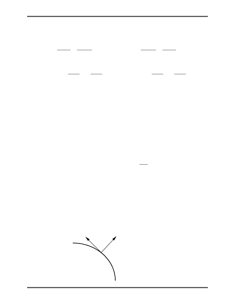
Lecture Notes: Introduction to Finite Element Method Chapter 5. Plate and Shell Elements
© 1999 Yijun Liu, University of Cincinnati
125
Shear forces and bending moments:
,
,
y
M
x
M
Q
y
M
x
M
Q
y
xy
y
xy
x
x
∂
∂
+
∂
∂
=
∂
∂
+
∂
∂
=
∂
∂
+
∂
∂
=
∂
∂
+
∂
∂
=
2
2
2
2
2
2
2
2
,
x
w
y
w
D
M
y
w
x
w
D
M
y
x
ν
ν
.
The fourth-order partial differential equation, given in (10)
and in terms of the deflection w(x,y), needs to be solved under
certain given boundary conditions.
Boundary Conditions:
Clamped:
0
,
0
=
∂
∂
=
n
w
w
;
(11)
Simply supported:
0
,
0
=
=
n
M
w
;
(12)
Free:
0
,
0
=
=
n
n
M
Q
;
(13)
where n is the normal direction of the boundary. Note that the
given values in the boundary conditions shown above can be
non-zero values as well.
boundary
n
s
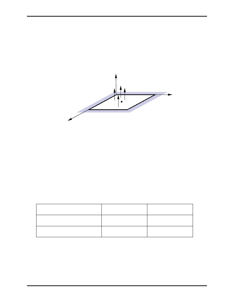
Lecture Notes: Introduction to Finite Element Method Chapter 5. Plate and Shell Elements
© 1999 Yijun Liu, University of Cincinnati
126
Examples:
A square plate with four edges clamped or hinged, and
under a uniform load q or a concentrated force P at the center C.
For this simple geometry, Eq. (10) with boundary condition
(11) or (12) can be solved analytically. The maximum
deflections are given in the following table for the different
cases.
Deflection at the Center (w
c
)
Clamped
Simply supported
Under uniform load q
0.00126 qL
4
/D
0.00406 qL
4
/D
Under concentrated force P
0.00560 PL
2
/D
0.0116 PL
2
/D
in which: D= Et
3
/(12(1-v
2
)).
These values can be used to verify the FEA solutions.
x
y
z
Given: E, t, and
ν
= 0.3
C
L
L
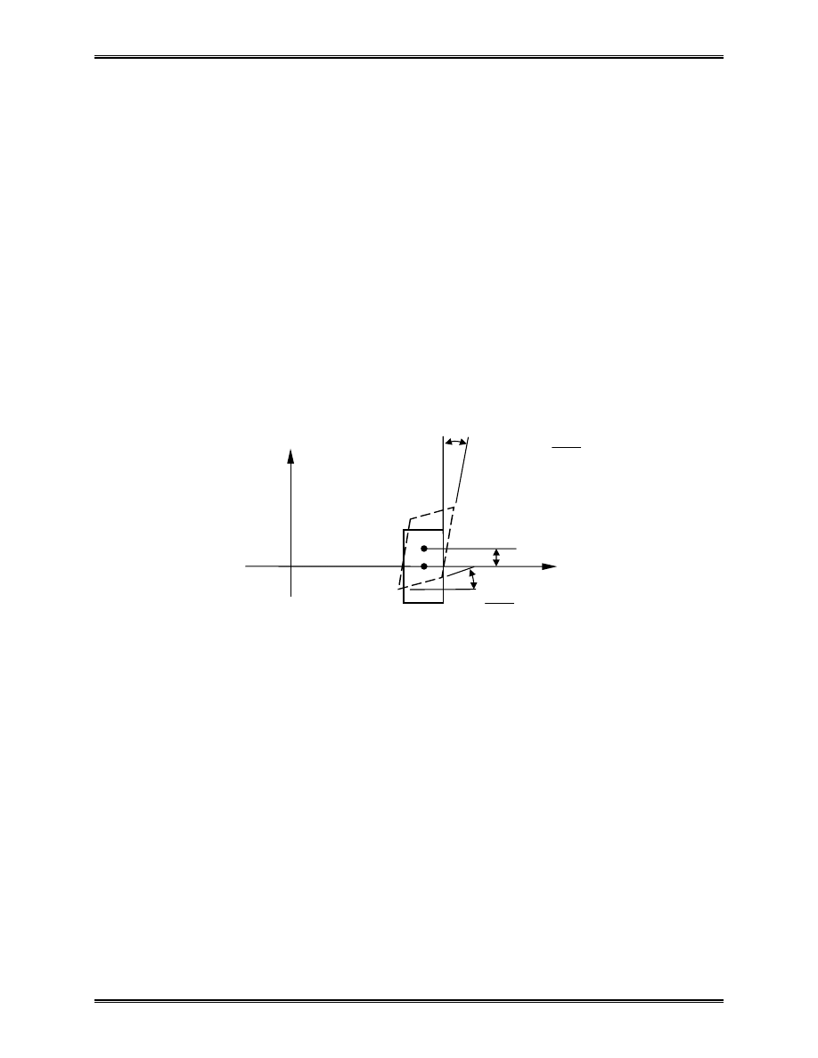
Lecture Notes: Introduction to Finite Element Method Chapter 5. Plate and Shell Elements
© 1999 Yijun Liu, University of Cincinnati
127
Thick Plate Theory (Mindlin Plate Theory)
If the thickness t of a plate is not “thin”, e.g.,
10
/
1
/
≥
L
t
(L = a characteristic dimension of the plate), then the thick plate
theory by Mindlin should be applied. This theory accounts for
the angle changes within a cross section, that is,
0
,
0
≠
≠
yz
xz
γ
γ
.
This means that a line which is normal to the mid surface before
the deformation will not be so after the deformation.
New independent variables:
x
θ
and
y
θ
: rotation angles of a line, which is normal to the
mid surface before the deformation, about x- and y-axis,
respectively.
x
z
w
x
w
∂
∂
∂
∂
−
≠
x
w
y
θ

Lecture Notes: Introduction to Finite Element Method Chapter 5. Plate and Shell Elements
© 1999 Yijun Liu, University of Cincinnati
128
New relations:
x
y
z
v
z
u
θ
θ
−
=
=
,
;
(14)
.
,
),
(
,
,
x
yz
y
xz
x
y
xy
x
y
y
x
y
w
x
w
x
y
z
y
z
x
z
θ
∂
∂
γ
θ
∂
∂
γ
∂
∂θ
∂
∂θ
γ
∂
∂θ
ε
∂
∂θ
ε
−
=
+
=
−
=
−
=
=
(15)
Note that if we imposed the conditions (or assumptions)
that
,
0
,
0
=
−
=
=
+
=
x
yz
y
xz
y
w
x
w
θ
∂
∂
γ
θ
∂
∂
γ
then we can recover the relations applied in the thin plate
theory.
Main variables:
)
,
(
and
)
,
(
),
,
(
y
x
y
x
y
x
w
y
x
θ
θ
.
The governing equations and boundary conditions can be
established for thick plate based on the above assumptions.
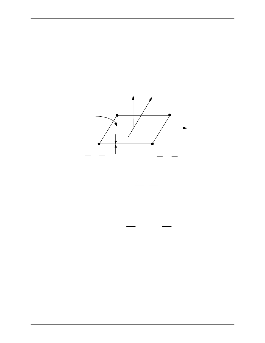
Lecture Notes: Introduction to Finite Element Method Chapter 5. Plate and Shell Elements
© 1999 Yijun Liu, University of Cincinnati
129
II. Plate Elements
Kirchhoff Plate Elements:
4-Node Quadrilateral Element
DOF at each node:
y
w
y
w
w
∂
∂
∂
∂
,
,
.
On each element, the deflection w(x,y) is represented by
∑
=
+
+
=
4
1
)
(
)
(
)
,
(
i
i
yi
i
xi
i
i
y
w
N
x
w
N
w
N
y
x
w
∂
∂
∂
∂
,
where N
i
, N
xi
and N
yi
are shape functions. This is an
incompatible element! The stiffness matrix is still of the form
∫
=
V
T
dV
EB
B
k
,
where B is the strain-displacement matrix, and E the stress-
strain matrix.
x
y
z
t
1
2
3
4
1
1
1
,
,
∂
∂
∂
∂
y
w
x
w
w
2
2
2
,
,
∂
∂
∂
∂
y
w
x
w
w
Mid surface
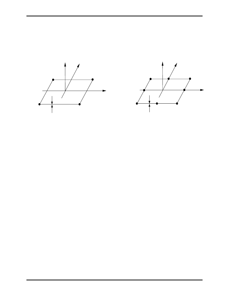
Lecture Notes: Introduction to Finite Element Method Chapter 5. Plate and Shell Elements
© 1999 Yijun Liu, University of Cincinnati
130
Mindlin Plate Elements:
4-Node Quadrilateral
8-Node Quadrilateral
DOF at each node:
w,
θ
x
and
θ
y
.
On each element:
.
)
,
(
,
)
,
(
,
)
,
(
1
1
1
∑
∑
∑
=
=
=
=
=
=
n
i
yi
i
y
n
i
xi
i
x
n
i
i
i
N
y
x
N
y
x
w
N
y
x
w
θ
θ
θ
θ
•
Three independent fields.
•
Deflection w(x,y) is linear for Q4, and quadratic for Q8.
x
y
z
t
1
2
3
4
x
y
z
t
1
2
3
4
5
6
7
8
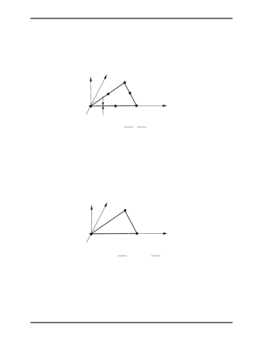
Lecture Notes: Introduction to Finite Element Method Chapter 5. Plate and Shell Elements
© 1999 Yijun Liu, University of Cincinnati
131
Discrete Kirchhoff Element:
Triangular plate element (not available in ANSYS).
Start with a 6-node triangular element,
DOF at corner nodes:
y
x
y
w
x
w
w
θ
θ
∂
∂
∂
∂
,
,
,
,
;
DOF at mid side nodes:
y
x
θ
θ
,
.
Total DOF = 21.
Then, impose conditions
0
=
=
yz
xz
γ
γ
, etc., at selected
nodes to reduce the DOF (using relations in (15)). Obtain:
At each node:
=
=
y
w
x
w
w
y
x
∂
∂
θ
∂
∂
θ
,
,
.
Total DOF = 9 (DKT Element).
•
Incompatible w(x,y); convergence is faster (w is cubic
along each edge) and it is efficient.
x
y
z
t
1
2
3
4
5
6
x
y
z
1
2
3
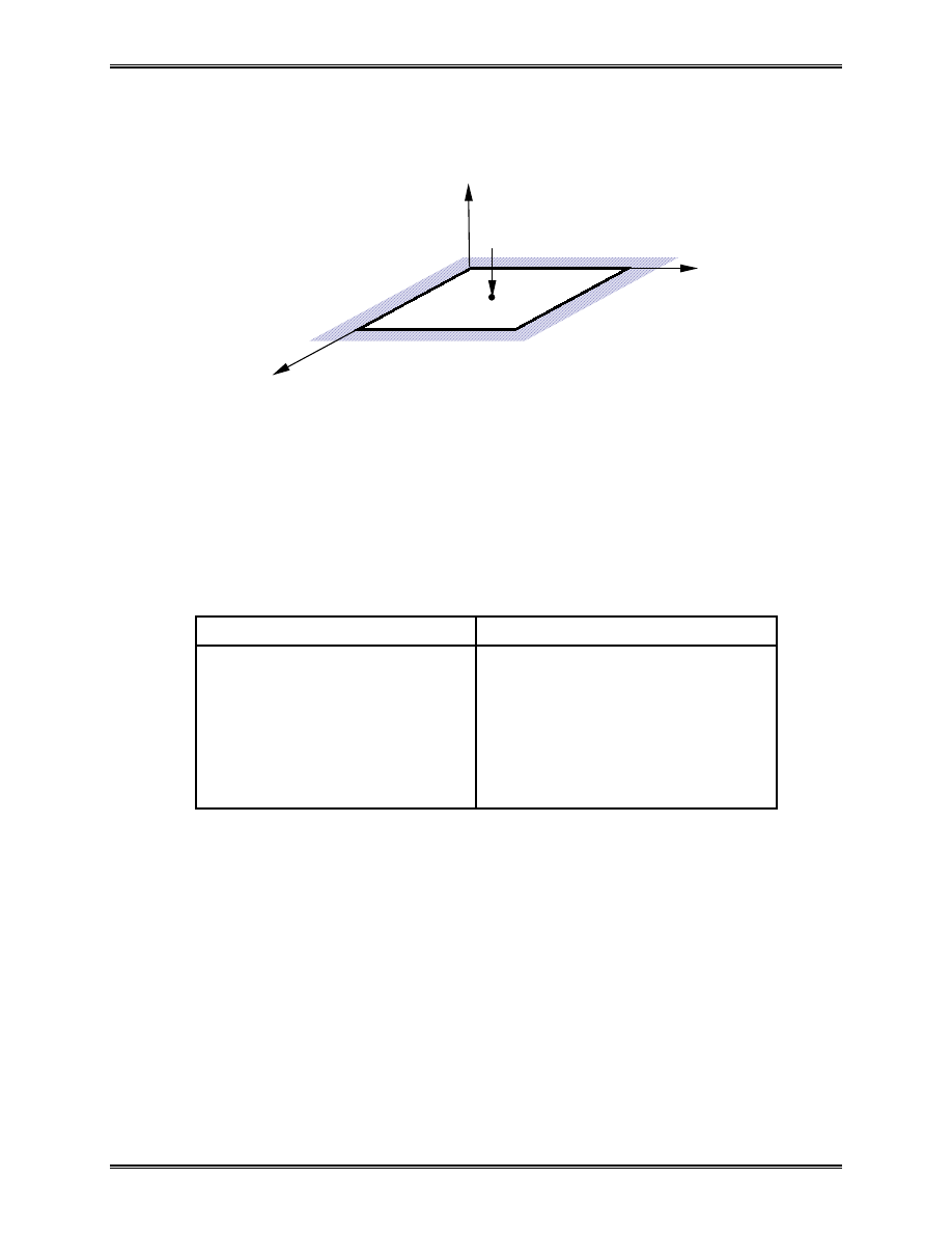
Lecture Notes: Introduction to Finite Element Method Chapter 5. Plate and Shell Elements
© 1999 Yijun Liu, University of Cincinnati
132
Test Problem:
ANSYS 4-node quadrilateral plate element.
ANSYS Result for w
c
Mesh
w
c
(
×
PL
2
/D)
2
×
2
0.00593
4
×
4
0.00598
8
×
8
0.00574
16
×
16
0.00565
:
:
Exact Solution
0.00560
Question: Converges from “above”? Contradiction to what
we learnt about the nature of the FEA solution?
Reason: This is an incompatible element ( See comments
on p. 177).
x
y
z
L/t = 10,
ν
= 0.3
C
L
L
P
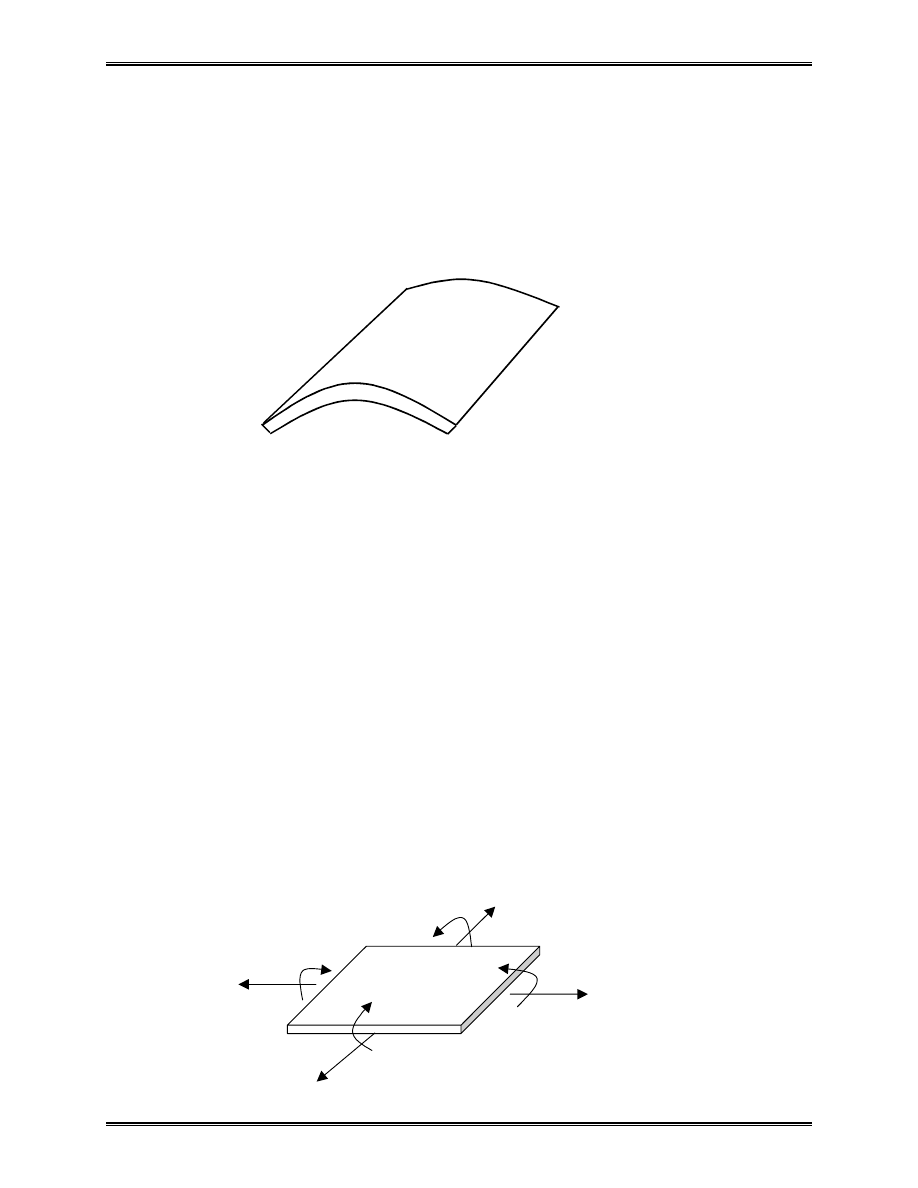
Lecture Notes: Introduction to Finite Element Method Chapter 5. Plate and Shell Elements
© 1999 Yijun Liu, University of Cincinnati
133
III. Shells and Shell Elements
Shells – Thin structures witch span over curved surfaces.
Example:
•
Sea shell, egg shell (the wonder of the nature);
•
Containers, pipes, tanks;
•
Car bodies;
•
Roofs, buildings (the Superdome), etc.
Forces in shells:
Membrane forces + Bending Moments
(cf. plates: bending only)
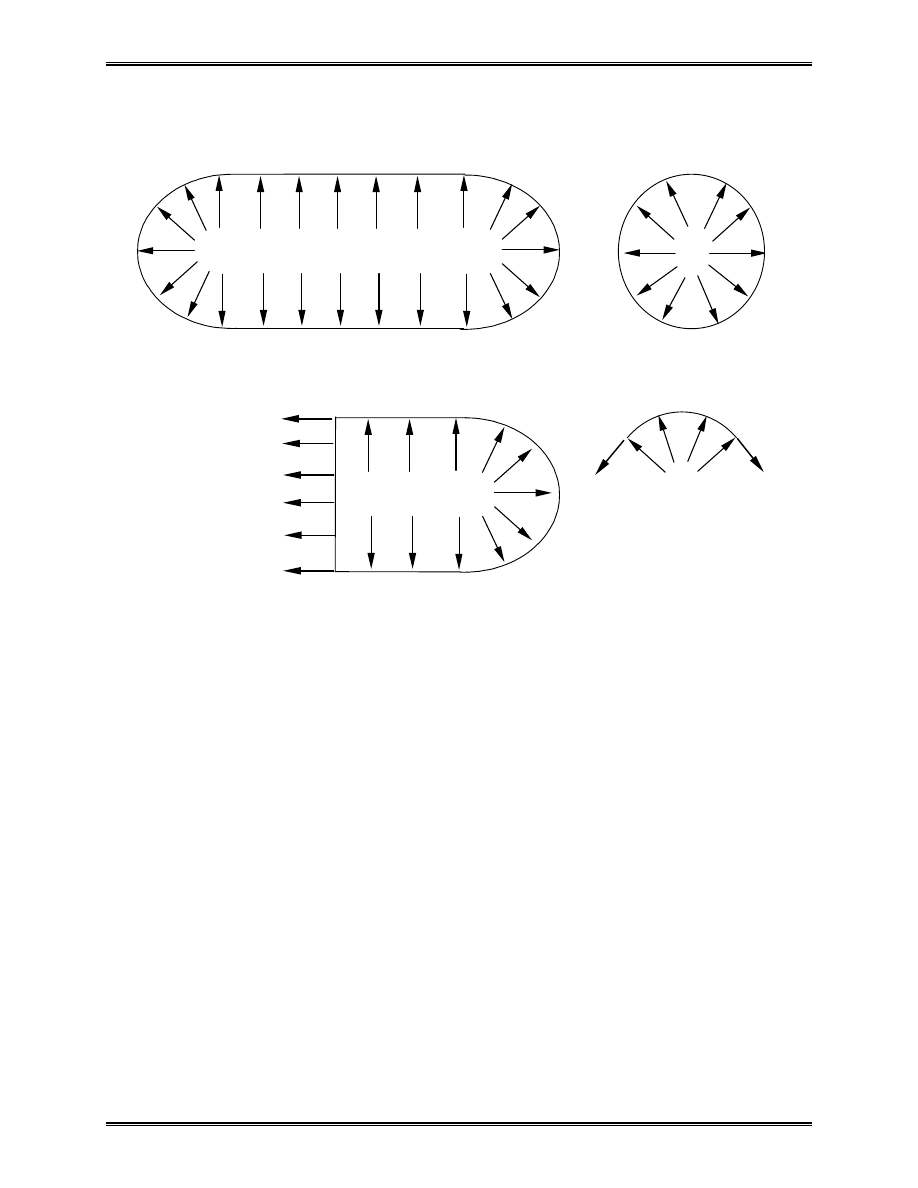
Lecture Notes: Introduction to Finite Element Method Chapter 5. Plate and Shell Elements
© 1999 Yijun Liu, University of Cincinnati
134
Example: A Cylindrical Container.
Shell Theory:
•
Thin shell theory
•
Thick shell theory
Shell theories are the most complicated ones to formulate
and analyze in mechanics (Russian’s contributions).
•
Engineering
≠
Craftsmanship
•
Demand strong analytical skill
p
p
internal forces:
membrane stresses
dominate
p
p
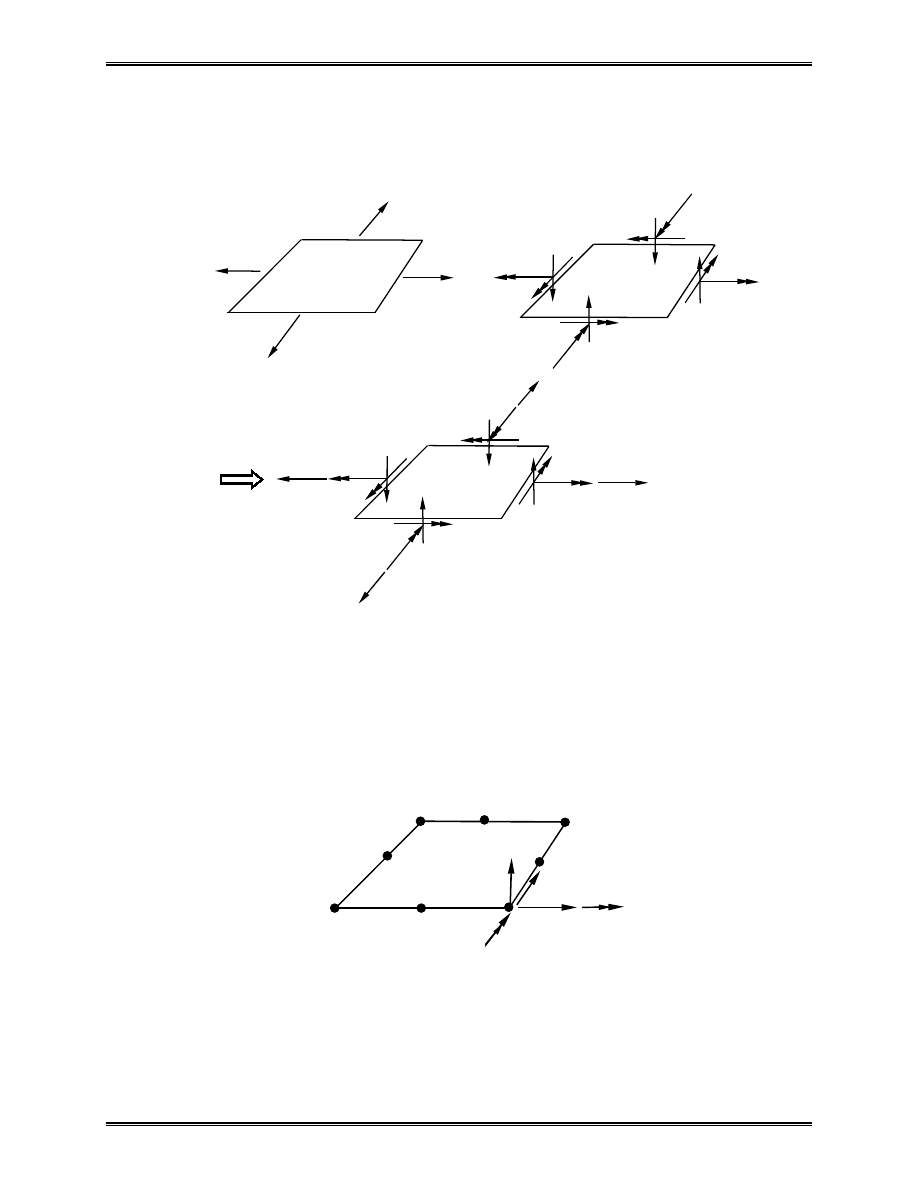
Lecture Notes: Introduction to Finite Element Method Chapter 5. Plate and Shell Elements
© 1999 Yijun Liu, University of Cincinnati
135
Shell Elements:
cf.: bar + simple beam element => general beam element.
DOF at each node:
Q4 or Q8 shell element.
+
plane stress element
plate bending element
flat shell element
u
v
w
θ
x
θ
y
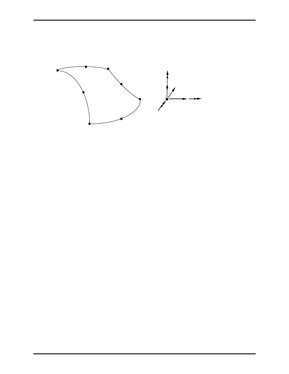
Lecture Notes: Introduction to Finite Element Method Chapter 5. Plate and Shell Elements
© 1999 Yijun Liu, University of Cincinnati
136
Curved shell elements:
•
Based on shell theories;
•
Most general shell elements (flat shell and plate
elements are subsets);
•
Complicated in formulation.
u
v
w
θ
x
θ
y
θ
z
i
i
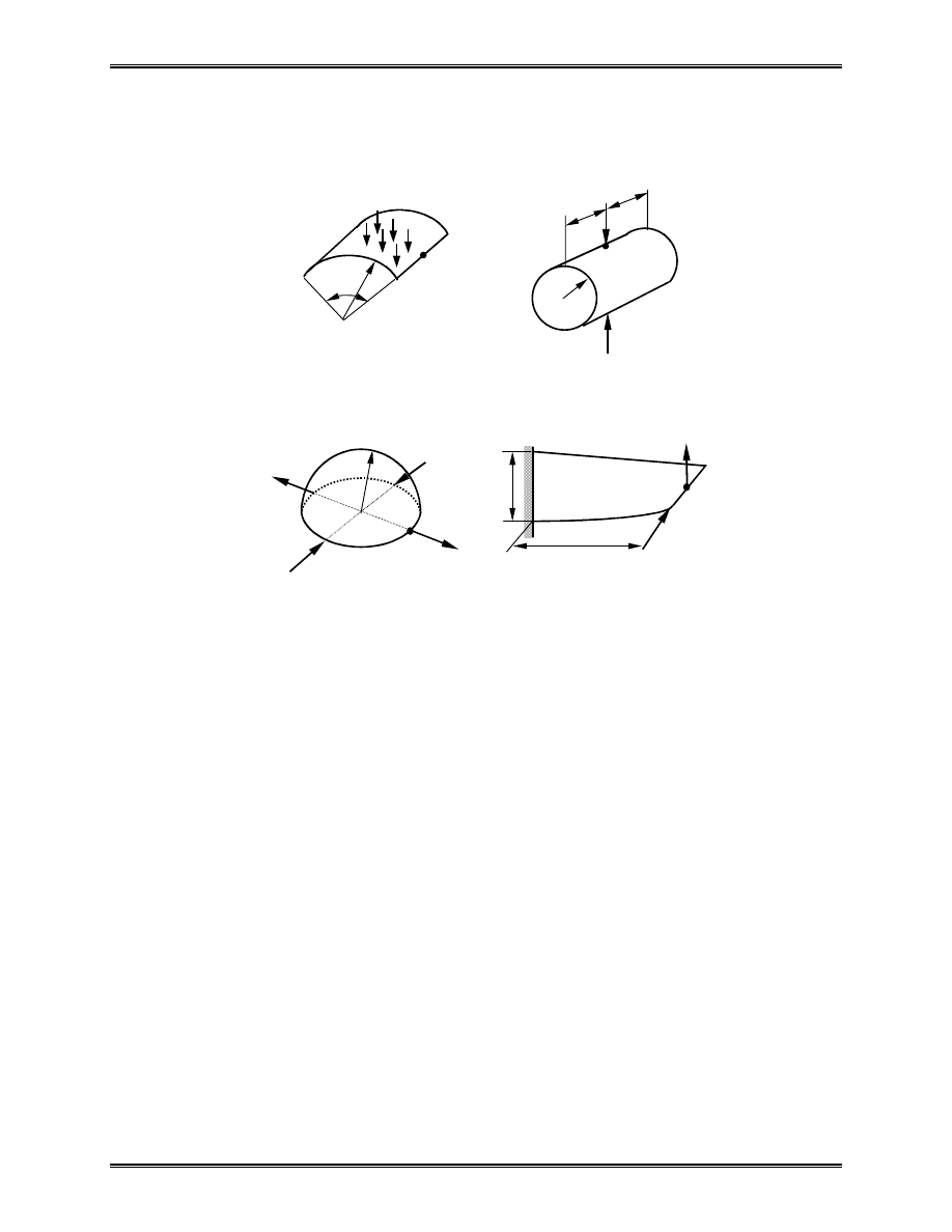
Lecture Notes: Introduction to Finite Element Method Chapter 5. Plate and Shell Elements
© 1999 Yijun Liu, University of Cincinnati
137
Test Cases:
ð
Check the Table, on page 188 of Cook’s book, for
values of the displacement
∆
A
under the various loading
conditions.
Difficulties in Application:
•
Non uniform thickness (turbo blades, vessels with
stiffeners, thin layered structures, etc.);
ð
Should turn to 3-D theory and apply solid elements.
A
R
80
o
Roof
R
A
F
F
L/2
L/2
Pinched Cylinder
A
F
F
F
F
R
Pinched Hemisphere
q
A
F
2
F
1
b
L
Twisted Strip (90
o
)
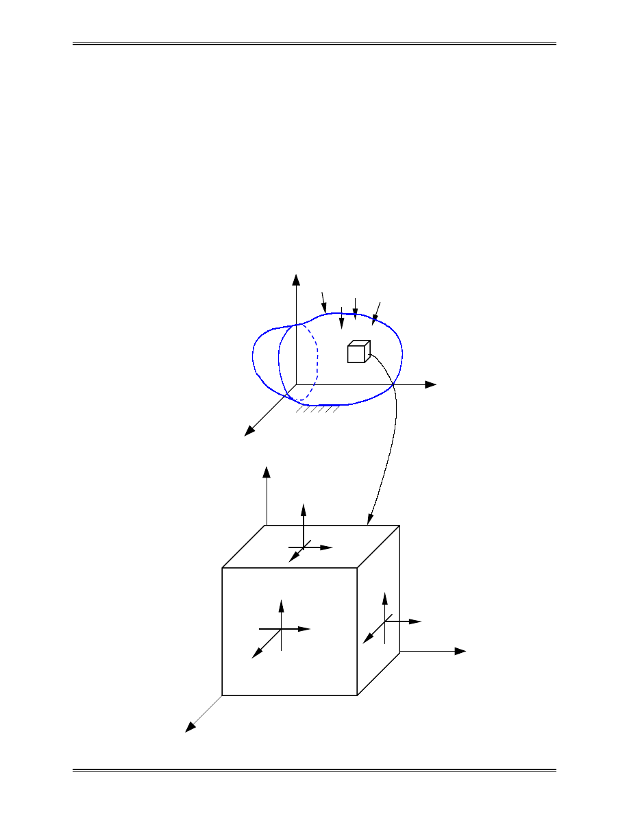
Lecture Notes: Introduction to Finite Element Method Chapter 6. Solid Elements
© 1999 Yijun Liu, University of Cincinnati
138
Chapter 6. Solid Elements for 3-D Problems
I. 3-D Elasticity Theory
Stress State:
y
F
x
z
y
σ
yx
τ
yz
τ
zy
τ
zx
τ
z
σ
xz
τ
x
σ
xy
τ
y , v
x, u
z, w

Lecture Notes: Introduction to Finite Element Method Chapter 6. Solid Elements
© 1999 Yijun Liu, University of Cincinnati
139
{ }
[ ]
)
1
(
,
ij
zx
yz
xy
z
y
x
or
σ
τ
τ
τ
σ
σ
σ
σ
=
=
ó
Strains:
{ }
[ ]
)
2
(
,
ij
zx
yz
xy
z
y
x
or
ε
γ
γ
γ
ε
ε
ε
ε
=
=
å
Stress-strain relation:
−
−
−
−
−
−
−
+
=
zx
yz
xy
z
y
x
zx
yz
xy
z
y
x
v
v
v
v
v
v
v
v
v
v
v
v
v
v
E
γ
γ
γ
ε
ε
ε
τ
τ
τ
σ
σ
σ
2
2
1
0
0
0
0
0
0
2
2
1
0
0
0
0
0
0
2
2
1
0
0
0
0
0
0
1
0
0
0
1
0
0
0
1
)
2
1
)(
1
(
or
)
3
(
E
å
ó
=

Lecture Notes: Introduction to Finite Element Method Chapter 6. Solid Elements
© 1999 Yijun Liu, University of Cincinnati
140
Displacement:
)
4
(
)
,
,
(
)
,
,
(
)
,
,
(
3
2
1
=
=
u
u
u
z
y
x
w
z
y
x
v
z
y
x
u
u
Strain-Displacement Relation:
)
5
(
,
,
,
,
,
x
w
z
u
z
v
y
w
y
u
x
v
z
w
y
v
x
u
xz
yz
xy
z
y
x
∂
∂
+
∂
∂
=
∂
∂
+
∂
∂
=
∂
∂
+
∂
∂
=
∂
∂
=
∂
∂
=
∂
∂
=
γ
γ
γ
ε
ε
ε
or
(
)
(
)
notation)
tensor
(
2
1
simply,
or
3
,
2
,
1
,
,
2
1
,
,
i
j
j
i
ij
i
j
j
i
ij
u
u
j
i
x
u
x
u
+
=
=
∂
∂
+
∂
∂
=
ε
ε
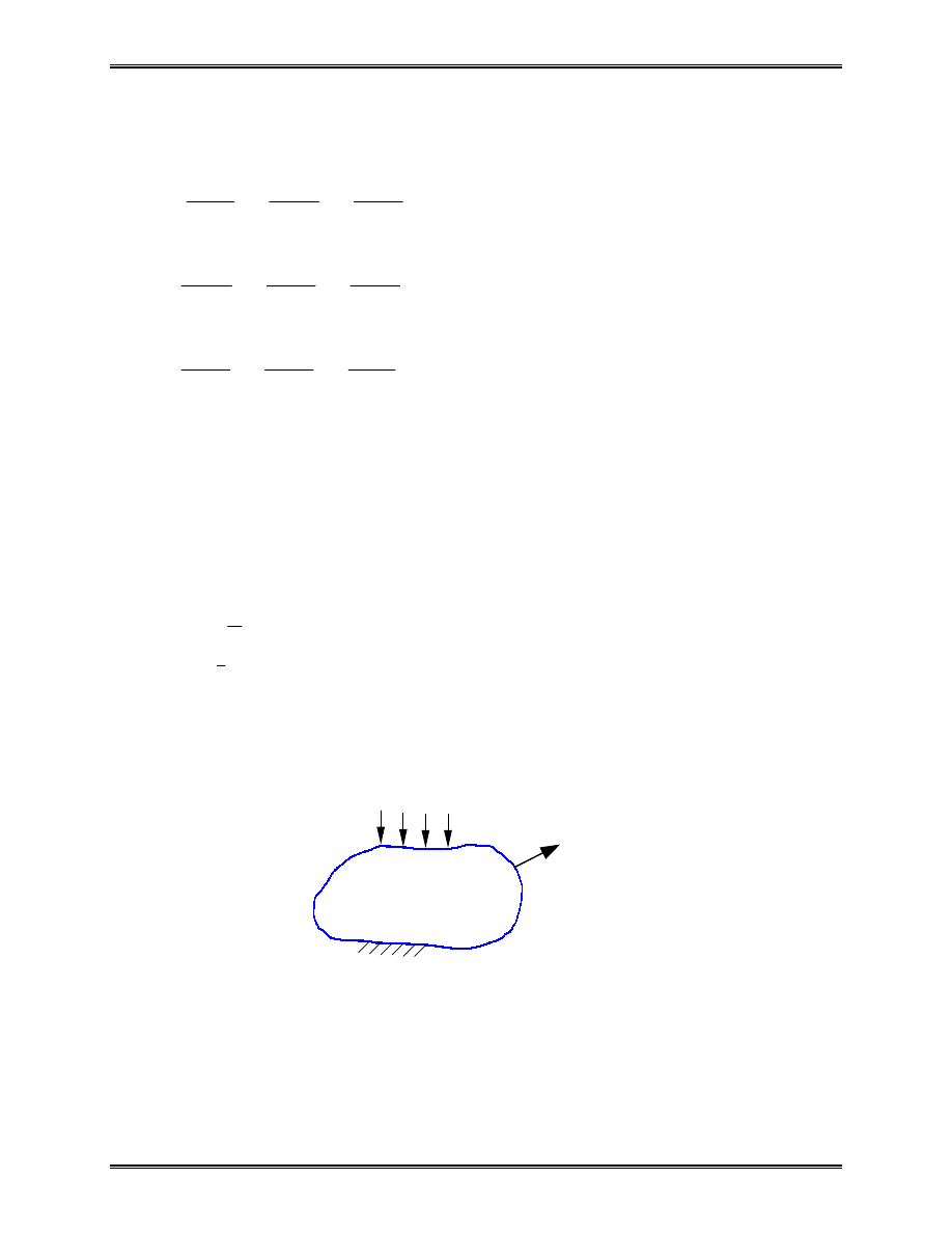
Lecture Notes: Introduction to Finite Element Method Chapter 6. Solid Elements
© 1999 Yijun Liu, University of Cincinnati
141
Equilibrium Equations:
0
or
,
0
)
6
(
,
0
,
0
,
=
+
=
+
∂
∂
+
∂
∂
+
∂
∂
=
+
∂
∂
+
∂
∂
+
∂
∂
=
+
∂
∂
+
∂
∂
+
∂
∂
i
j
ij
z
z
zy
zx
y
yz
y
yx
x
xz
xy
x
f
f
z
y
x
f
z
y
x
f
z
y
x
σ
σ
τ
τ
τ
σ
τ
τ
τ
σ
Boundary Conditions (BC’s):
)
traction
(
)
7
(
)
(
,
)
(
,
j
ij
i
i
i
u
i
i
n
t
traction
specified
on
t
t
nt
displaceme
specified
on
u
u
σ
σ
=
Γ
=
Γ
=
Stress Analysis:
Solving equations in (6) under the BC’s in (7).
p
n
σ
Γ
u
Γ
)
(
σ
Γ
+
Γ
=
Γ
u
Lecture Notes: Introduction to Finite Element Method Chapter 6. Solid Elements
© 1999 Yijun Liu, University of Cincinnati
142
II. Finite Element Formulation
Displacement Field:
i
N
i
i
i
N
i
i
N
i
i
i
w
N
w
v
N
v
u
N
u
∑
∑
∑
=
=
=
=
=
=
1
1
1
)
8
(
Nodal values
In matrix form:
)
9
(
)
1
3
(
)
3
3
(
)
1
3
(
2
2
2
1
1
1
2
1
2
1
2
1
0
0
0
0
0
0
0
0
0
0
0
0
×
×
×
=
N
N
w
v
u
w
v
u
N
N
N
N
N
N
w
v
u
M
L
L
L
or
d
N
u
=
Using relations (5) and (8), we can derive the strain vector
ε
=B d
(6
×
1) (6
×
3N)
×
(3N
×
1)

Lecture Notes: Introduction to Finite Element Method Chapter 6. Solid Elements
© 1999 Yijun Liu, University of Cincinnati
143
Stiffness Matrix:
)
10
(
∫
=
v
T
dv
B
E
B
k
(3
×
N) (3N
×
6)
×
(6
×
6)
×
(6
×
3N)
Numerical quadratures are often needed to evaluate the
above integration.
Rigid-body motions for 3-D bodies (6 components):
3 translations, 3 rotations.
These rigid-body motions (singularity of the system of
equations) must be removed from the FEA model to ensure the
quality of the analysis.
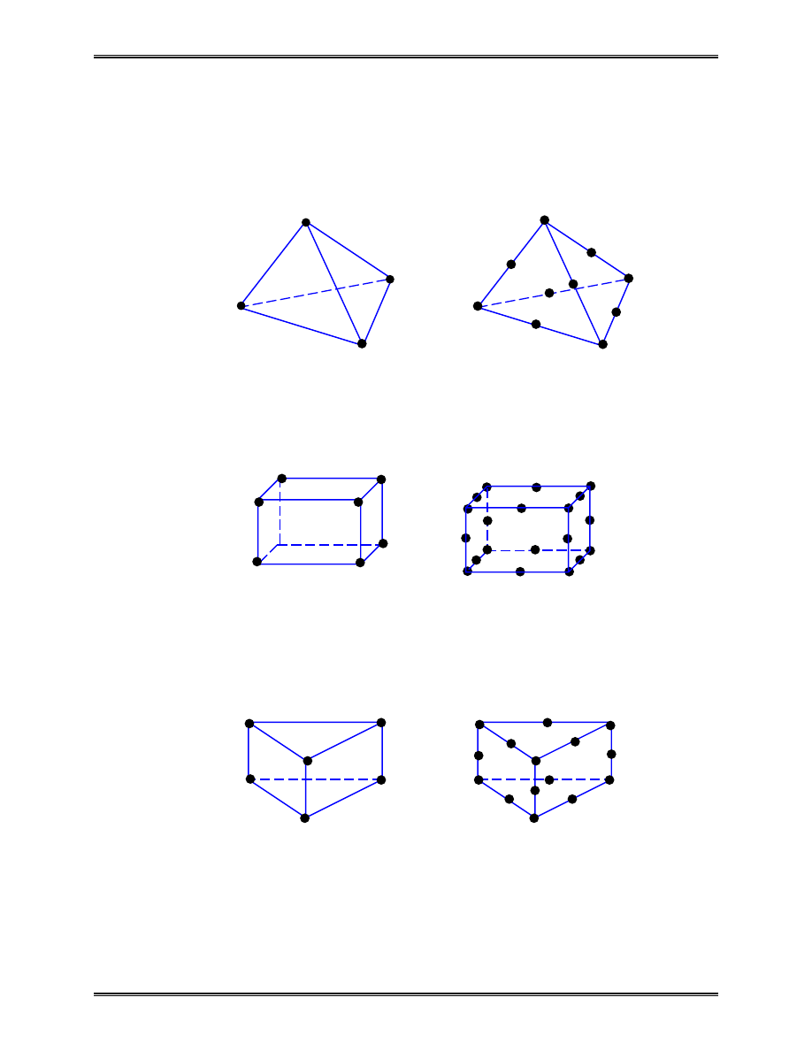
Lecture Notes: Introduction to Finite Element Method Chapter 6. Solid Elements
© 1999 Yijun Liu, University of Cincinnati
144
III Typical 3-D Solid Elements
Tetrahedron:
Hexahedron (brick):
Penta:
Avoid using the linear (4-node) tetrahedron element in 3-D
stress analysis (Inaccurate! But it is OK for dynamic analysis).
linear (4 nodes) quadratic (10 nodes)
linear (8 nodes) quadratic (20 nodes)
linear (6 nodes) quadratic (15 nodes)
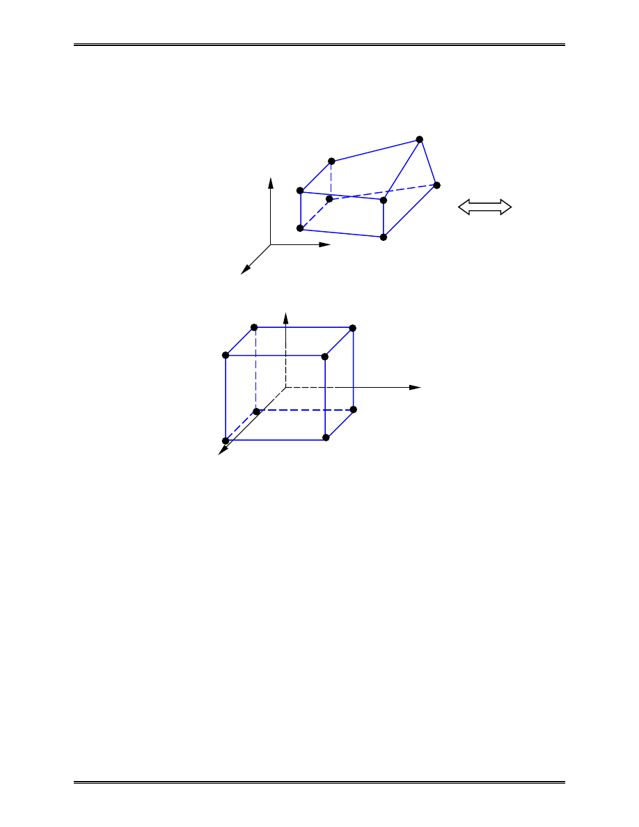
Lecture Notes: Introduction to Finite Element Method Chapter 6. Solid Elements
© 1999 Yijun Liu, University of Cincinnati
145
Element Formulation:
Linear Hexahedron Element
Displacement field in the element:
)
11
(
,
,
8
1
8
1
1
8
1
∑
∑
∑
=
=
=
=
=
=
i
i
i
i
i
i
i
i
i
w
N
w
v
N
v
u
N
u
6
5
y 8
7
2
1
4
3
mapping (x
↔ξ
)
x (-1
≤
ξ
,
η
,
ζ
≤
1)
z
η
(-1,1,-1) 4 3 (1,1,-1)
(-1,1,1) 8
7 (1,1,1)
o
ξ
(-1,-1,-1) 1
2 (1,-1,-1)
(-1,-1,1) 5
6 (1,-1,1)
ζ

Lecture Notes: Introduction to Finite Element Method Chapter 6. Solid Elements
© 1999 Yijun Liu, University of Cincinnati
146
Shape functions:
.
)
1
(
)
1
(
)
1
(
8
1
)
,
,
(
)
12
(
,
)
1
(
)
1
(
)
1
(
8
1
)
,
,
(
,
)
1
(
)
1
(
)
1
(
8
1
)
,
,
(
,
)
1
(
)
1
(
)
1
(
8
1
)
,
,
(
8
3
2
1
ζ
η
ξ
ζ
η
ξ
ζ
η
ξ
ζ
η
ξ
ζ
η
ξ
ζ
η
ξ
ζ
η
ξ
ζ
η
ξ
+
+
−
=
−
+
+
=
−
−
+
=
−
−
−
=
N
N
N
N
M
M
Note that we have the following relations for the shape
functions:
.
1
)
,
,
(
.
8
,
,
2
,
1
,
,
)
,
,
(
8
1
∑
=
=
=
=
i
i
ij
j
j
j
i
N
j
i
N
ζ
η
ξ
δ
ζ
η
ξ
L
Coordinate Transformation (Mapping):
)
13
(
.
,
,
8
1
8
1
8
1
∑
∑
∑
=
=
=
=
=
=
i
i
i
i
i
i
i
i
i
z
N
z
y
N
y
x
N
x
The same shape functions are used as for the displacement
field.
⇒
Isoparametric element.

Lecture Notes: Introduction to Finite Element Method Chapter 6. Solid Elements
© 1999 Yijun Liu, University of Cincinnati
147
Jacobian Matrix:
matrix
Jacobian
z
u
y
u
x
u
z
y
x
z
y
x
z
y
x
u
u
u
J
≡
∂
∂
∂
∂
∂
∂
∂
∂
∂
∂
∂
∂
∂
∂
∂
∂
∂
∂
∂
∂
∂
∂
∂
∂
=
∂
∂
∂
∂
∂
∂
)
14
(
ζ
ζ
ζ
η
η
η
ξ
ξ
ξ
ζ
η
ξ
⇒
∂
∂
=
∂
∂
∂
∂
∂
∂
∂
∂
=
∂
∂
∂
∂
∂
∂
∑
=
−
.
,
,
8
1
1
etc
u
N
u
u
u
u
z
u
y
u
x
u
i
i
i
ξ
ξ
ζ
η
ξ
J
and
)
15
(
,
1
∂
∂
∂
∂
∂
∂
=
∂
∂
∂
∂
∂
∂
−
ζ
η
ξ
v
v
v
z
v
y
v
x
v
J
also for w.

Lecture Notes: Introduction to Finite Element Method Chapter 6. Solid Elements
© 1999 Yijun Liu, University of Cincinnati
148
⇒
where d is the nodal displacement vector,
i.e.,
)
16
(
d
B
å
=
(6
×
1) (6
×
24)
×
(24
×
1)
d
B
å
=
=
∂
∂
+
∂
∂
∂
∂
+
∂
∂
∂
∂
+
∂
∂
∂
∂
∂
∂
∂
∂
=
=
)
15
(
use
zx
yz
xy
z
y
x
x
w
z
u
z
v
y
w
y
u
x
x
z
w
y
v
x
u
L
γ
γ
γ
ε
ε
ε

Lecture Notes: Introduction to Finite Element Method Chapter 6. Solid Elements
© 1999 Yijun Liu, University of Cincinnati
149
Strain energy,
)
17
(
2
1
2
1
)
(
2
1
2
1
d
B
E
B
d
å
E
å
å
E
å
å
ó
=
=
=
=
∫
∫
∫
∫
V
T
T
V
T
V
T
V
T
dV
dV
dV
dV
U
Element stiffness matrix,
)
18
(
∫
=
V
T
dV
B
E
B
k
(24
×
24) (24
×
6)
×
(6
×
6)
×
(6
×
24)
In
ξηζ
coordinates:
)
19
(
)
det
(
ζ
η
ξ
d
d
d
dV
J
=
⇒
)
20
(
)
(det
1
1
1
1
1
1
∫ ∫ ∫
− − −
=
ζ
η
ξ
d
d
d
T
J
B
E
B
k
( Numerical integration)
•
3-D elements usually do not use rotational DOFs.
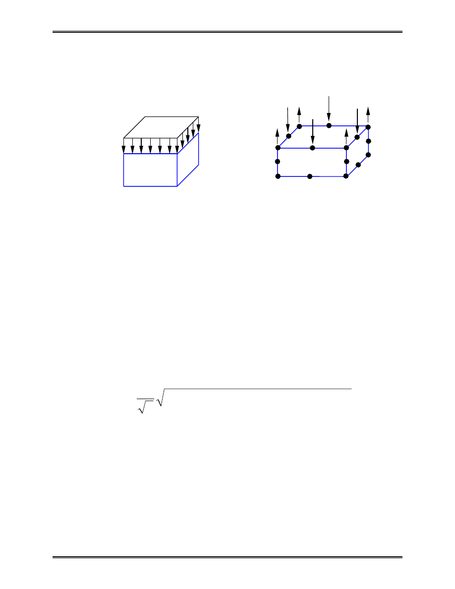
Lecture Notes: Introduction to Finite Element Method Chapter 6. Solid Elements
© 1999 Yijun Liu, University of Cincinnati
150
Loads:
Distributed loads
⇒
Nodal forces
Area =A Nodal forces for 20-node
Hexahedron
Stresses:
d
B
E
å
E
ó
=
=
Principal stresses:
.
,
,
3
2
1
σ
σ
σ
von Mises stress:
2
1
3
2
3
2
2
2
1
)
(
)
(
)
(
2
1
σ
σ
σ
σ
σ
σ
σ
σ
−
+
−
+
−
=
=
VM
e
.
Stresses are evaluated at selected points (including nodes)
on each element. Averaging (around a node, for example) may
be employed to smooth the field.
Examples: …
pA/3 pA/12
p
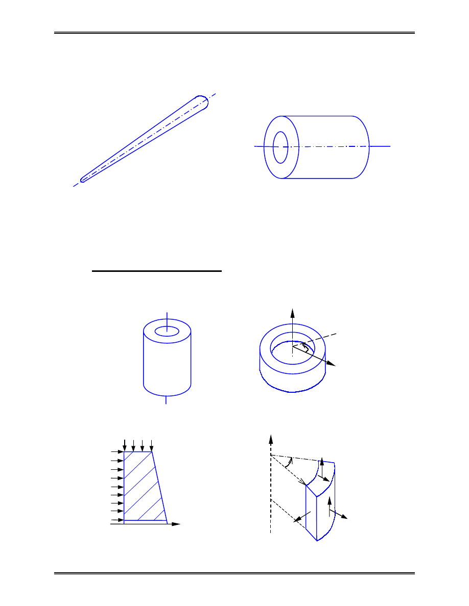
Lecture Notes: Introduction to Finite Element Method Chapter 6. Solid Elements
© 1999 Yijun Liu, University of Cincinnati
151
Solids of Revolution (Axisymmetric Solids):
Baseball bat shaft
Apply cylindrical coordinates:
( x, y, z)
⇒
(r,
θ
, z)
θ
r, u
z,w
z, w
θ
r, u
θ
σ
z
σ
rz
τ
r
σ
r
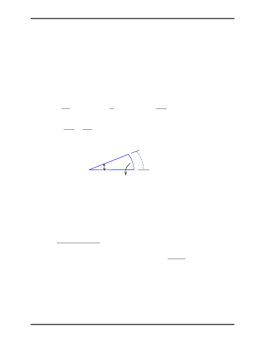
Lecture Notes: Introduction to Finite Element Method Chapter 6. Solid Elements
© 1999 Yijun Liu, University of Cincinnati
152
Displacement field:
(
)
component
ntial
circumfere
No
)
,
(
,
)
,
(
−
=
=
v
z
r
w
w
z
r
u
u
Strains:
)
21
(
)
0
(
,
,
,
,
=
=
∂
∂
+
∂
∂
=
∂
∂
=
=
∂
∂
=
θ
θ
θ
γ
γ
γ
ε
ε
ε
z
r
rz
z
r
z
u
r
w
z
w
r
u
r
u
Stresses:
)
22
(
2
2
1
0
0
0
0
1
0
1
0
1
)
2
1
(
)
1
(
−
−
−
−
−
+
=
rz
z
r
rz
z
r
v
v
v
v
v
v
v
v
v
v
v
v
E
γ
ε
ε
ε
τ
σ
σ
σ
θ
θ
d
θ
r
(r+u)d
θ
rd
θ
u
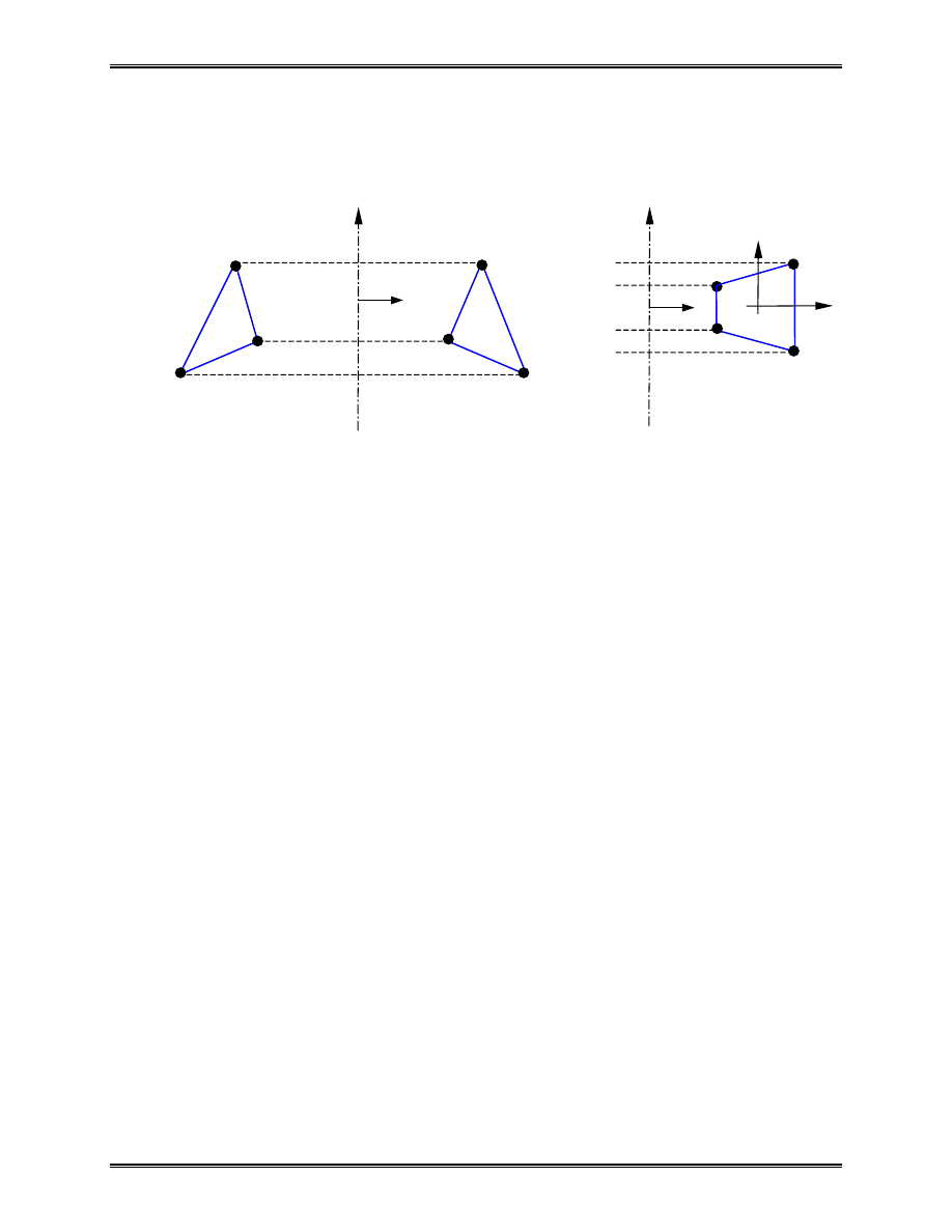
Lecture Notes: Introduction to Finite Element Method Chapter 6. Solid Elements
© 1999 Yijun Liu, University of Cincinnati
153
Axisymmetric Elements:
)
23
(
∫
=
V
T
dz
d
rdr
θ
B
E
B
k
or
)
24
(
)
(det
2
)
(det
1
1
1
1
2
0
1
1
1
1
η
ξ
π
θ
η
ξ
π
d
d
r
d
d
d
r
T
T
∫∫
∫∫∫
− −
− −
=
=
J
B
E
B
J
B
E
B
k
r, u
3
2
4
1
ξ
η
r, u
2
3
1
1
2
3
3-node element (ring)
4-node element (ring)
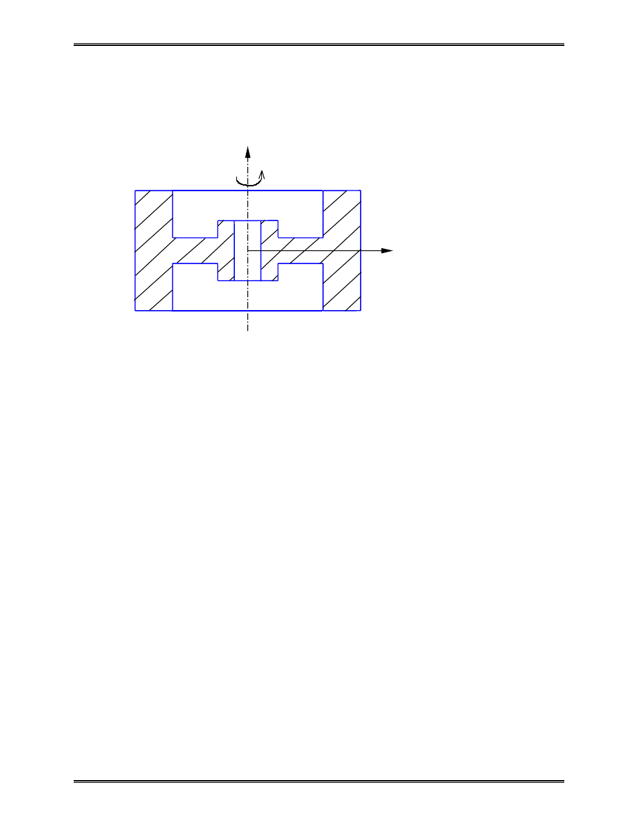
Lecture Notes: Introduction to Finite Element Method Chapter 6. Solid Elements
© 1999 Yijun Liu, University of Cincinnati
154
Applications:
•
Rotating Flywheel:
Body forces:
)
force
nal
gravitatio
(
)
force
inertial
l/
centrifuga
radial
equivalent
(
2
g
f
r
f
z
r
ρ
ω
ρ
−
=
=
z
ω
angular velocity (rad/s)
r
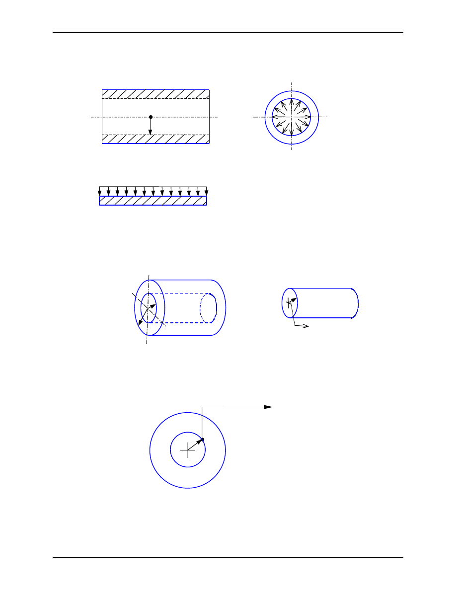
Lecture Notes: Introduction to Finite Element Method Chapter 6. Solid Elements
© 1999 Yijun Liu, University of Cincinnati
155
•
Cylinder Subject to Internal Pressure:
•
Press Fit:
ring ( Sleeve) shaft
p
0
r
0
2
)
(
r
p
q
π
=
0
r
i
r
δ
+
i
r
“i” “o”
MPC
u
u
i
o
⇒
=
−
δ
:
i
r
r
at
=
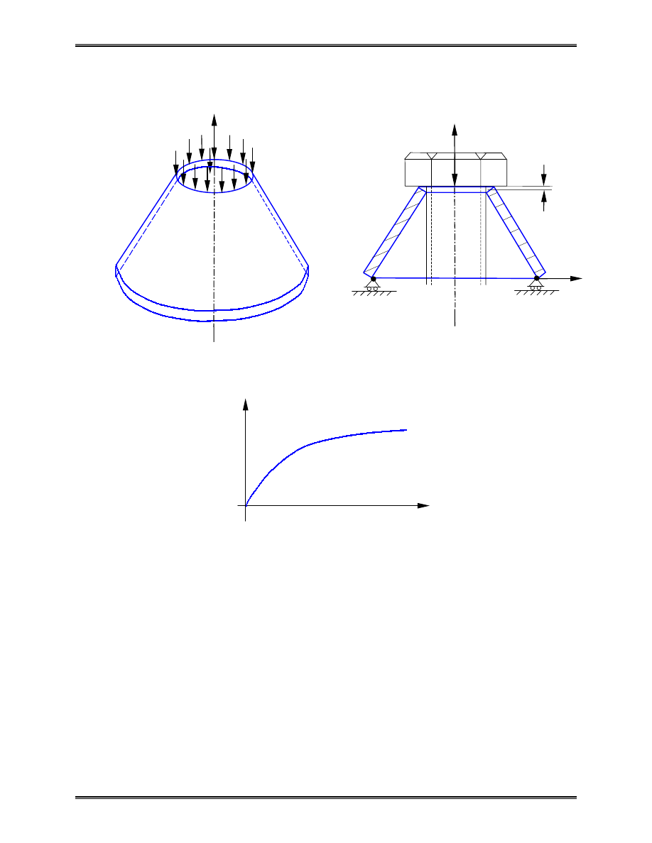
Lecture Notes: Introduction to Finite Element Method Chapter 6. Solid Elements
© 1999 Yijun Liu, University of Cincinnati
156
•
Belleville (Conical) Spring:
This is a geometrically nonlinear (large deformation)
problem and iteration method (incremental approach) needs to
be employed.
p
p
δ
z
δ
r
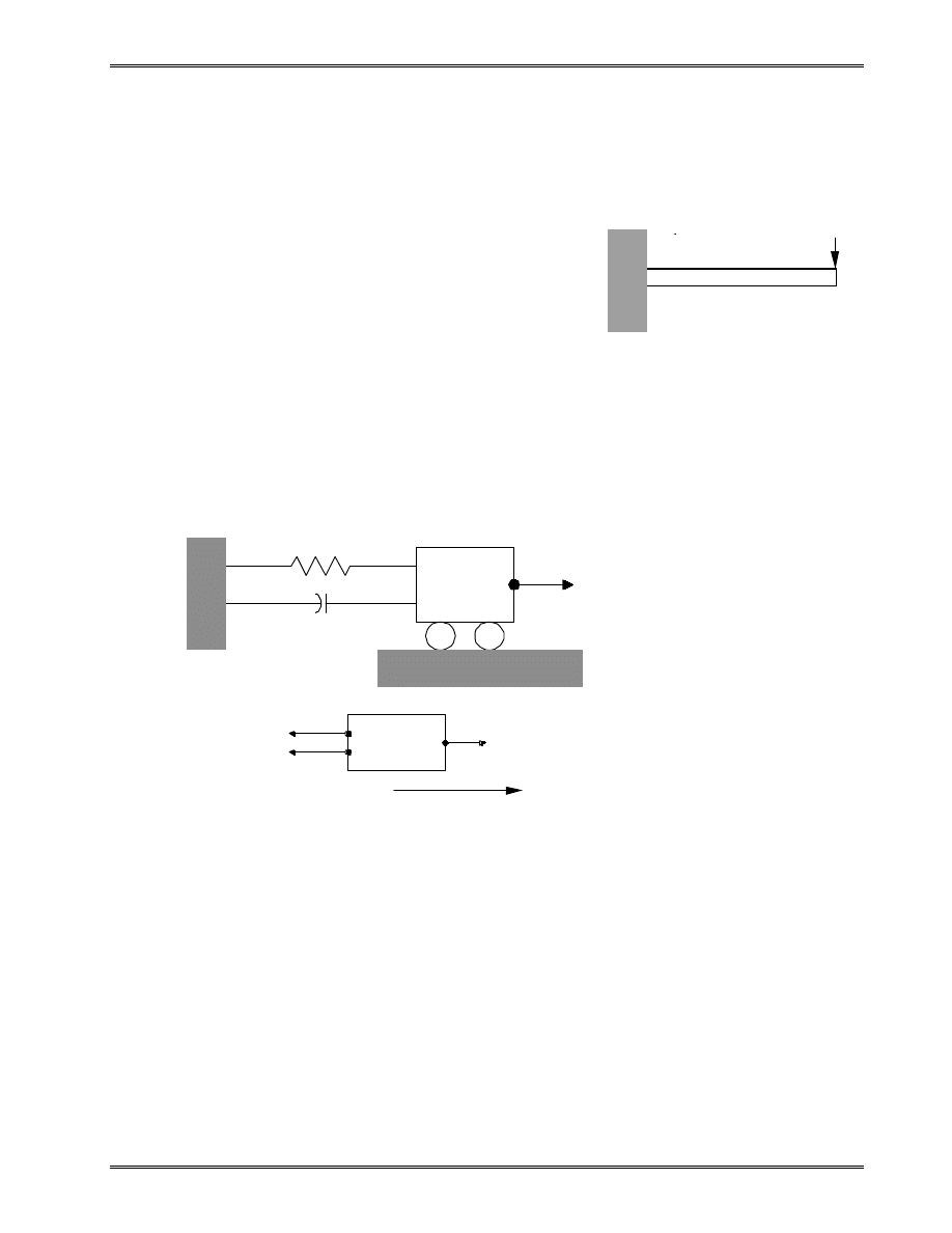
Lecture Notes: Introduction to Finite Element Method Chapter 7. Structural Vibration and Dynamics
© 1999 Yijun Liu, University of Cincinnati
157
Chapter 7. Structural Vibration and Dynamics
•
Natural frequencies and modes
•
Frequency response (F(t)=F
o
sin
ωt)
•
Transient response (F(t) arbitrary)
I. Basic Equations
A. Single DOF System
From Newton’s law of motion (ma = F), we have
u
c
u
k
f(t)
u
m
&
&&
−
−
=
,
i.e.
f(t)
u
k
u
c
u
m
=
+
+
&
&&
, (1)
where u is the displacement,
dt
du
u
/
=
&
and
.
/
2
2
dt
u
d
u
=
&
&
F(t)
m
m
f=f(t)
k
c
f(t)
u
c
ku
&
force
-
)
(
damping
-
stiffness
-
mass
-
t
f
c
k
m
x, u

Lecture Notes: Introduction to Finite Element Method Chapter 7. Structural Vibration and Dynamics
© 1999 Yijun Liu, University of Cincinnati
158
Free Vibration:
f(t) = 0 and no damping (c = 0)
Eq. (1) becomes
0
=
+
u
k
u
m &
&
.
(2)
(meaning: inertia force + stiffness force = 0)
Assume:
t)
(
U
u(t)
ω
sin
=
,
where
ω
is the frequency of oscillation, U the amplitude.
Eq. (2) yields
0
sin
sin
2
=
+
−
t)
ù
(
U
k
t)
ù
(
m
ù
U
i.e.,
[
]
0
2
=
+
−
U
k
m
ω
.
For nontrivial solutions for U, we must have
[
]
0
2
=
+
−
k
m
ω
,
which yields
m
k
=
ω
.
(3)
This is the circular natural frequency of the single DOF
system (rad/s). The cyclic frequency (1/s = Hz) is
π
ω
2
=
f
,
(4)
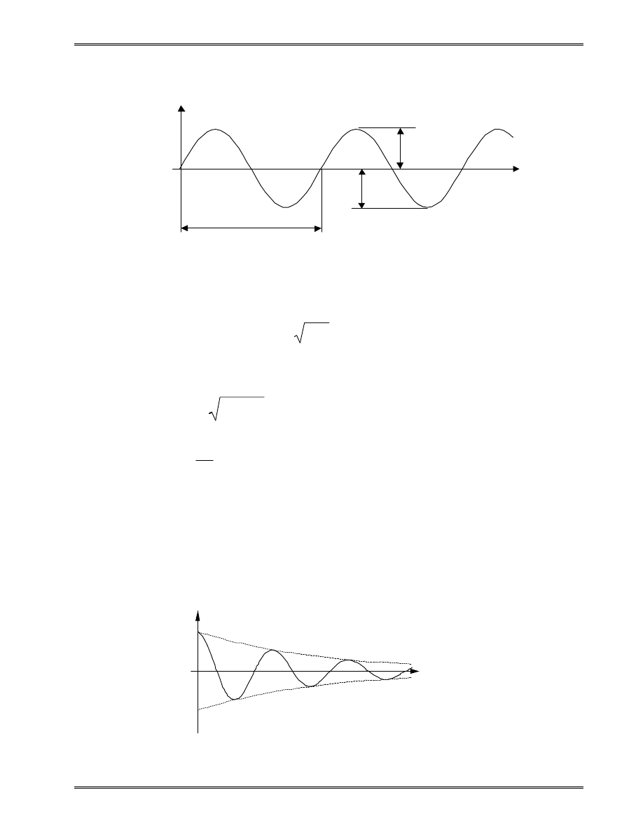
Lecture Notes: Introduction to Finite Element Method Chapter 7. Structural Vibration and Dynamics
© 1999 Yijun Liu, University of Cincinnati
159
With non-zero damping c, where
m
k
m
c
c
c
2
2
0
=
=
<
<
ω
(c
c
= critical damping) (5)
we have the damped natural frequency:
2
1
ξ
ω
ω
−
=
d
,
(6)
where
c
c
c
=
ξ
(damping ratio).
For structural damping:
15
.
0
0
<
≤
ξ
(usually 1~5%)
ω
ω
≈
d
.
(7)
Thus, we can ignore damping in normal mode analysis.
u
t
U
U
T = 1 / f
U n d a m p e d F r e e V i b r a t i o n
u = U s i n w t
u
t
Damped Free Vibration
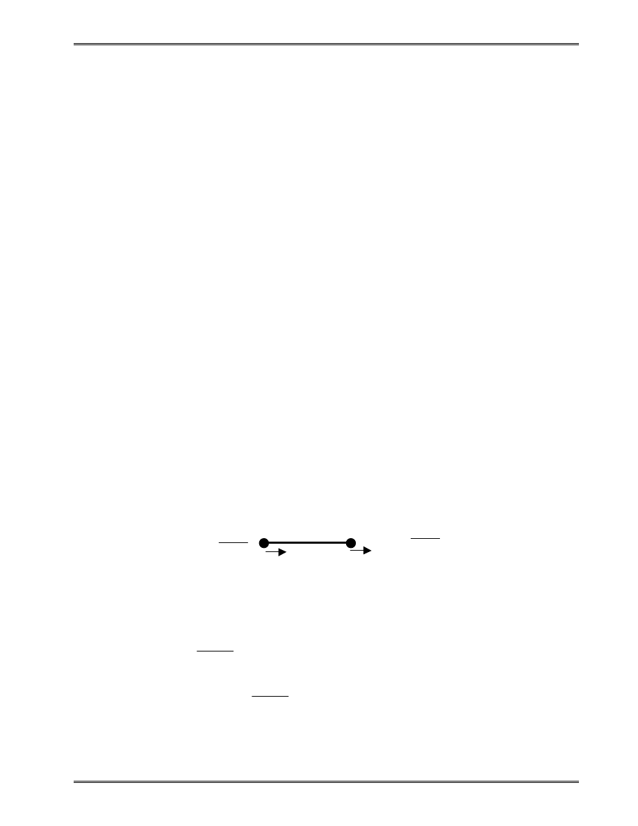
Lecture Notes: Introduction to Finite Element Method Chapter 7. Structural Vibration and Dynamics
© 1999 Yijun Liu, University of Cincinnati
160
B. Multiple DOF System
Equation of Motion
Equation of motion for the whole structure is
)
(t
f
Ku
u
C
u
M
=
+
+
&
&
&
,
(8)
in which:
u
nodal displacement vector,
M
mass matrix,
C
damping matrix,
K
stiffness matrix,
f
forcing vector.
Physical meaning of Eq. (8):
Inertia forces + Damping forces + Elastic forces
= Applied forces
Mass Matrices
Lumped mass matrix (1-D bar element):
1
ρ,A,L 2
u
1
u
2
Element mass matrix is found to be
4
4 3
4
4 2
1
matrix
diagonal
2
0
0
2
=
AL
AL
ρ
ρ
m
2
1
AL
m
ρ
=
2
2
AL
m
ρ
=

Lecture Notes: Introduction to Finite Element Method Chapter 7. Structural Vibration and Dynamics
© 1999 Yijun Liu, University of Cincinnati
161
In general, we have the consistent mass matrix given by
dV
V
T
∫
=
N
N
m
ρ
(9)
where N is the same shape function matrix as used for the
displacement field.
This is obtained by considering the kinetic energy:
( )
( ) ( )
u
N
N
u
u
N
u
N
u
m
u
m
&
43
42
1
&
&
&
&
&
&
&
&
∫
∫
∫
∫
=
=
=
=
=
Κ
V
T
T
V
T
V
T
V
T
dV
dV
dV
u
u
dV
u
mv
ρ
ρ
ρ
ρ
2
1
2
1
2
1
2
1
)
2
1
(cf.
2
1
2
2
Bar Element (linear shape function):
[
]
3
/
1
6
/
1
6
/
1
3
/
1
1
1
2
1
u
u
AL
ALd
V
&
&
&
&
=
−
−
=
∫
ρ
ξ
ξ
ξ
ξ
ξ
ρ
m
(10)
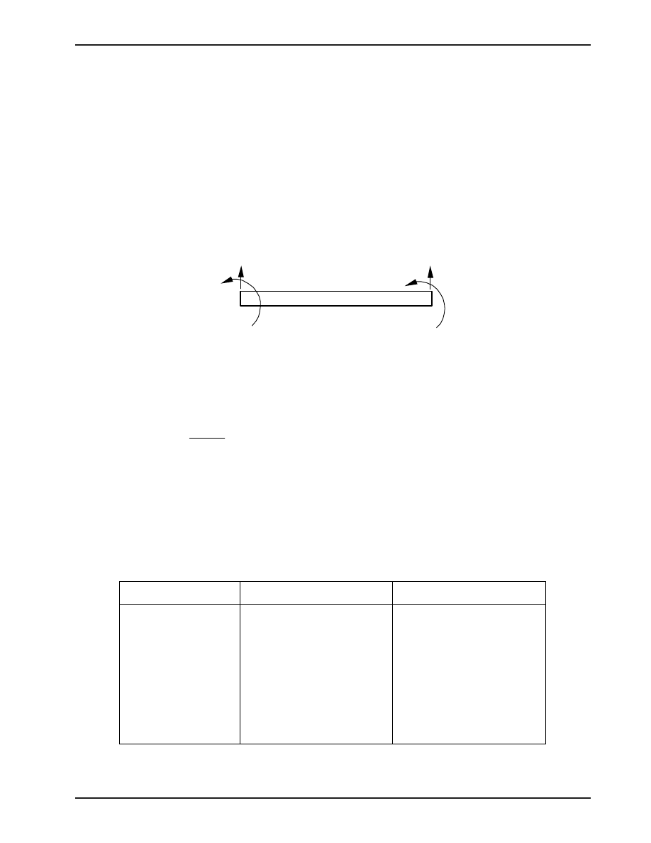
Lecture Notes: Introduction to Finite Element Method Chapter 7. Structural Vibration and Dynamics
© 1999 Yijun Liu, University of Cincinnati
162
Element mass matrices:
⇒
local coordinates
⇒
to global coordinates
⇒
assembly of the global structure mass matrix M.
Simple Beam Element:
4
22
3
13
22
156
13
54
3
13
4
22
13
54
22
156
420
2
2
1
1
2
2
2
2
θ
θ
ρ
ρ
&
&
&
&
&
&
&
&
v
v
L
L
L
L
L
L
L
L
L
L
L
L
AL
dV
T
−
−
−
−
−
−
=
=
∫
V
N
N
m
(11)
Units in dynamic analysis (make sure they are consistent):
Choice I
Choice II
t (time)
L (length)
m (mass)
a (accel.)
f (force)
ρ (density)
s
m
kg
m/s
2
N
kg/m
3
s
mm
Mg
mm/s
2
N
Mg/mm
3
1
1
θ
v
2
2
θ
v
ρ, A, L

Lecture Notes: Introduction to Finite Element Method Chapter 7. Structural Vibration and Dynamics
© 1999 Yijun Liu, University of Cincinnati
163
II. Free Vibration
Study of the dynamic characteristics of a structure:
•
natural frequencies
•
normal modes (shapes)
Let f(t) = 0 and C = 0 (ignore damping) in the dynamic
equation (8) and obtain
0
Ku
u
M
=
+
&
&
(12)
Assume that displacements vary harmonically with time, that
is,
),
sin(
)
(
),
cos(
)
(
),
sin(
)
(
2
t
t
t
t
t
t
ω
ω
ω
ω
ω
u
u
u
u
u
u
−
=
=
=
&
&
&
where
u
is the vector of nodal displacement amplitudes.
Eq. (12) yields,
[
]
0
u
M
K
=
−
2
ω
(13)
This is a generalized eigenvalue problem (EVP).
Solutions?

Lecture Notes: Introduction to Finite Element Method Chapter 7. Structural Vibration and Dynamics
© 1999 Yijun Liu, University of Cincinnati
164
Trivial solution:
0
u
=
for any values of
ω
(not interesting).
Nontrivial solutions:
0
u
≠
only if
0
2
=
−
M
K
ω
(14)
This is an n-th order polynomial of
ω
2
, from which we can
find n solutions (roots) or eigenvalues
ω
i
.
• ω
i
(i = 1, 2, …, n) are the natural frequencies (or
characteristic frequencies) of the structure.
• ω
1
(the smallest one) is called the fundamental frequency.
•
For each
ω
i
, Eq. (13) gives one solution (or eigen) vector
[
]
0
u
M
K
=
−
i
i
2
ω
.
i
u
(i=1,2,…,n) are the normal modes (or natural
modes, mode shapes, etc.).
Properties of Normal Modes
0
=
j
T
i
u
K
u
,
0
=
j
T
i
u
M
u
, for i
≠ j, (15)
if
j
i
ω
ω
≠
. That is, modes are orthogonal (or independent) to
each other with respect to K and M matrices.

Lecture Notes: Introduction to Finite Element Method Chapter 7. Structural Vibration and Dynamics
© 1999 Yijun Liu, University of Cincinnati
165
Normalize the modes:
.
,
1
2
i
i
T
i
i
T
i
ω
=
=
u
K
u
u
M
u
(16)
Note:
•
Magnitudes of displacements (modes) or stresses in normal
mode analysis have no physical meaning.
•
For normal mode analysis, no support of the structure is
necessary.
ω
i
= 0
⇔
there are rigid body motions of the whole or a
part of the structure.
⇒
apply this to check the FEA model (check for
mechanism or free elements in the models).
•
Lower modes are more accurate than higher modes in the
FE calculations (less spatial variations in the lower modes
⇒
fewer elements/wave length are needed).
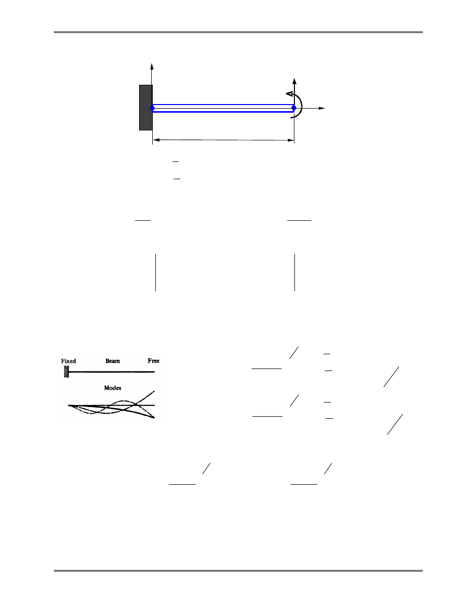
Lecture Notes: Introduction to Finite Element Method Chapter 7. Structural Vibration and Dynamics
© 1999 Yijun Liu, University of Cincinnati
166
Example:
[
]
.
4
22
22
156
420
,
4
6
6
12
,
0
0
2
2
3
2
2
2
−
−
=
−
−
=
=
−
L
L
L
AL
L
L
L
L
EI
v
ρ
θ
ω
M
K
M
K
EVP:
in which
EI
AL
420
/
4
2
ρ
ω
λ
=
.
Solving the EVP, we obtain,
Exact solutions:
.
03
.
22
,
516
.
3
2
1
4
2
2
1
4
1
=
=
AL
EI
AL
EI
ρ
ω
ρ
ω
We can see that mode 1 is calculated much more accurately
than mode 2, with one beam element.
L
x
1
2
v
2
ρ, A, EI
y
θ
2
,
0
4
4
22
6
22
6
156
12
2
2
=
−
+
−
+
−
−
λ
λ
λ
λ
L
L
L
L
L
L
.
62
.
7
1
v
,
81
.
34
,
38
.
1
1
v
,
533
.
3
2
2
2
2
1
4
2
1
2
2
2
1
4
1
=
=
=
=
L
AL
EI
L
AL
EI
θ
ρ
ω
θ
ρ
ω
#1
#2
#3
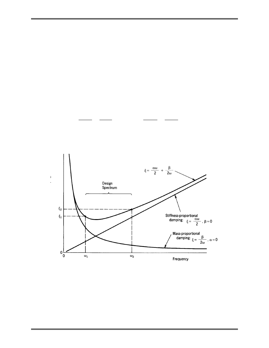
Lecture Notes: Introduction to Finite Element Method Chapter 7. Structural Vibration and Dynamics
© 1999 Yijun Liu, University of Cincinnati
167
III. Damping
Two commonly used models for viscous damping.
A.
Proportional Damping (Rayleigh Damping)
K
M
C
β
α
+
=
(17)
where the constants
α
&
β
are found from
,
2
2
,
2
2
2
2
2
1
1
1
ω
β
αω
ξ
ω
β
αω
ξ
+
=
+
=
with
2
1
2
1
&
,
,
ξ
ξ
ω
ω
(damping ratio) being selected.
B. Modal Damping
Incorporate the viscous damping in modal equations.
Dam
p
ing
r
a
ti
o

Lecture Notes: Introduction to Finite Element Method Chapter 7. Structural Vibration and Dynamics
© 1999 Yijun Liu, University of Cincinnati
168
IV. Modal Equations
•
Use the normal modes (modal matrix) to transform the
coupled system of dynamic equations to uncoupled
system of equations.
We have
[
]
n
1,2,...,
,
2
=
=
−
i
i
i
0
u
M
K
ω
(18)
where the normal mode
i
u satisfies:
=
=
,
0
,
0
j
T
i
j
T
i
u
M
u
u
K
u
for
i
≠
j,
and
=
=
,
,
1
2
i
i
T
i
i
T
i
ω
u
K
u
u
M
u
for i = 1, 2, …, n.
Form the modal matrix:
[
]
n
n
n
u
u
u
Ö
2
1
)
(
L
=
×
(19)
Can verify that
.
,
matrix)
Spectral
(
0
0
0
0
0
0
2
n
2
2
2
1
I
M
Ö
Ö
Ù
K
Ö
Ö
=
=
=
T
T
ω
ω
ω
L
O
M
M
L
(20)

Lecture Notes: Introduction to Finite Element Method Chapter 7. Structural Vibration and Dynamics
© 1999 Yijun Liu, University of Cincinnati
169
Transformation for the displacement vector,
z
u
u
u
u
Φ
=
+
+
+
=
n
n
z
z
z
L
2
2
1
1
, (21)
where
=
)
(
)
(
)
(
2
1
t
z
t
z
t
z
n
M
z
are called principal coordinates.
Substitute (21) into the dynamic equation:
Pre-multiply by
Φ
T
, and apply (20):
),
( t
p
z
z
C
z
=
Ω
+
+
&
&&
φ
(22)
where
Ω
+
=
β
α
φ
I
C
(proportional damping),
)
( t
T
f
p
Φ
=
.
Using Modal Damping
=
n
n
ω
ξ
ω
ξ
ω
ξ
φ
2
0
2
0
0
0
2
2
2
1
1
L
M
O
M
L
C
. (23)
).
( t
f
z
K
z
C
z
M
=
Φ
+
Φ
+
Φ
&
&
&

Lecture Notes: Introduction to Finite Element Method Chapter 7. Structural Vibration and Dynamics
© 1999 Yijun Liu, University of Cincinnati
170
Equation (22) becomes,
),
(
2
2
t
p
z
z
z
i
i
i
i
i
i
i
=
+
+
ω
ω
ξ
&
&&
i = 1,2,…,n. (24)
Equations in (22) or (24) are called modal equations.
These are uncoupled, second-order differential equations,
which are much easier to solve than the original dynamic
equation (coupled system).
To recover u from z, apply transformation (21) again, once
z is obtained from (24).
Notes:
•
Only the first few modes may be needed in constructing
the modal matrix
Φ
(i.e.,
Φ
could be an n
×
m rectangular
matrix with m<n). Thus, significant reduction in the
size of the system can be achieved.
•
Modal equations are best suited for problems in which
higher modes are not important (i.e., structural
vibrations, but not shock loading).
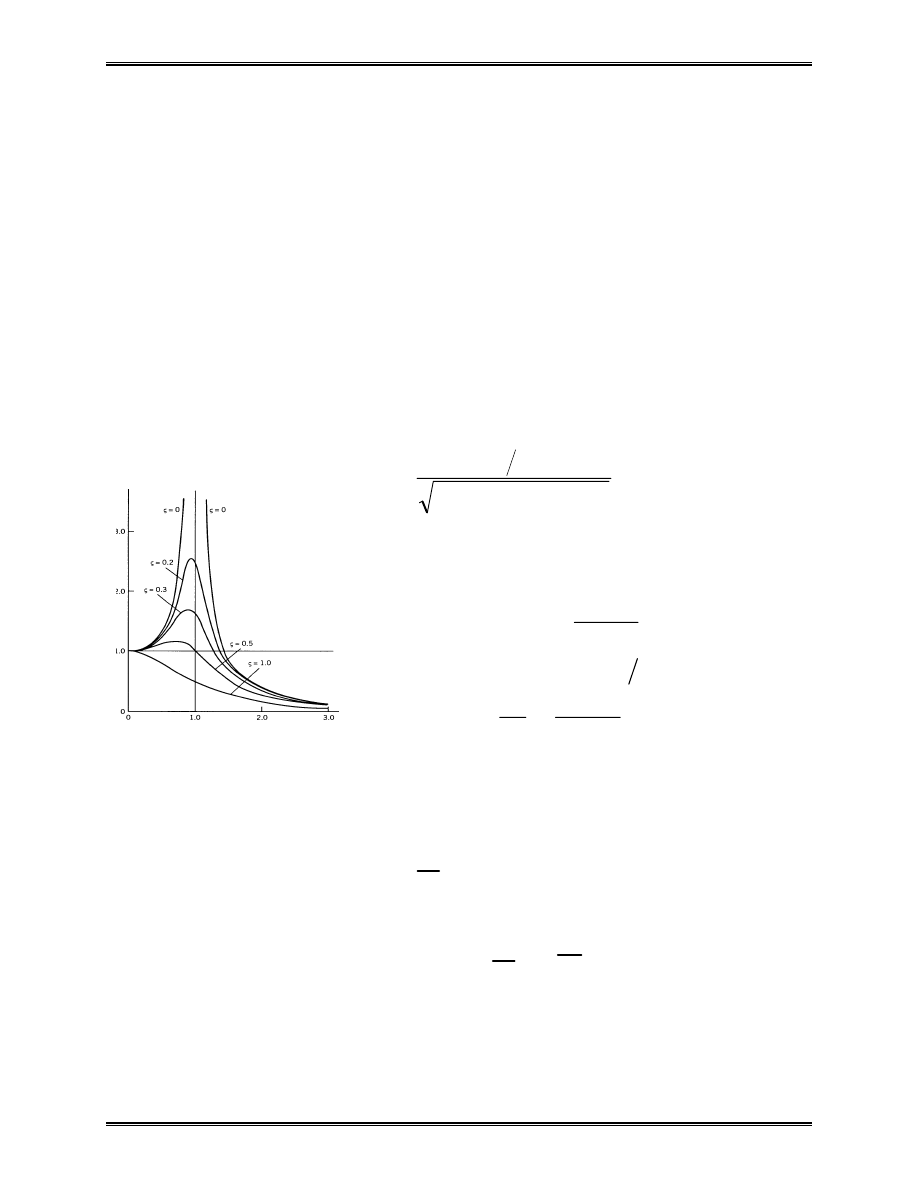
Lecture Notes: Introduction to Finite Element Method Chapter 7. Structural Vibration and Dynamics
© 1999 Yijun Liu, University of Cincinnati
171
V. Frequency Response Analysis
(Harmonic Response Analysis)
3
2
1
&
&&
loading
Harmonic
sin t
ω
F
Ku
u
C
u
M
=
+
+
(25)
Modal method: Apply the modal equations,
,
sin
2
2
t
p
z
z
z
i
i
i
i
i
i
i
ω
ω
ω
ξ
=
+
+
&
&&
i=1,2,…,m. (26)
These are 1-D equations. Solutions are
),
sin(
)
2
(
)
1
(
)
(
2
2
2
2
i
i
i
i
i
i
i
t
p
t
z
θ
ω
η
ξ
η
ω
−
+
−
=
(27)
where
=
=
=
−
=
ratio
damping
,
2
,
angle
phase
,
1
2
arctan
i
2
i
i
c
i
i
i
i
i
i
i
m
c
c
c
ω
ξ
ω
ω
η
η
η
ξ
θ
Recover u from (21).
Direct Method: Solve Eq. (25) directly, that is, calculate
the inverse. With
t
i
e
ω
u
u
=
(complex notation), Eq. (25)
becomes
[
]
.
2
F
u
M
C
K
=
−
+
ω
ω
i
This equation is expensive to solve and matrix is ill-
conditioned if
ω
is close to any
ω
i
.
z
i
ω
/
ω
i
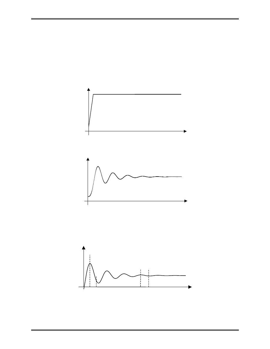
Lecture Notes: Introduction to Finite Element Method Chapter 7. Structural Vibration and Dynamics
© 1999 Yijun Liu, University of Cincinnati
172
VI. Transient Response Analysis
(Dynamic Response/Time-History Analysis)
•
Structure response to arbitrary, time-dependent loading.
f(t)
t
u(t)
t
Compute responses by integrating through time:
t
0
t
1
t
2
t
n
t
n+1
u
1
u
2
u
n
u
n+1
t

Lecture Notes: Introduction to Finite Element Method Chapter 7. Structural Vibration and Dynamics
© 1999 Yijun Liu, University of Cincinnati
173
Equation of motion at instance
n
t , n = 0, 1, 2, 3,
⋅⋅⋅
:
.
n
n
n
n
f
Ku
u
C
u
M
=
+
+
&
&&
Time increment:
∆
t=t
n+1
-t
n
, n=0, 1, 2, 3,
⋅⋅⋅
.
There are two categories of methods for transient analysis.
A. Direct Methods (Direct Integration Methods)
•
Central Difference Method
Approximate using finite difference:
)
2
(
)
(
1
),
(
2
1
1
1
2
1
1
−
+
−
+
+
−
∆
=
−
∆
=
n
n
n
n
n
n
n
t
t
u
u
u
u
u
u
u
&
&
&
Dynamic equation becomes,
,
)
(
2
1
)
2
(
)
(
1
1
1
1
1
2
n
n
n
n
n
n
n
t
t
f
Ku
u
u
C
u
u
u
M
=
+
−
∆
+
+
−
∆
−
+
−
+
which yields,
)
(
1
t
n
F
Au
=
+
where
( )
( )
( )
∆
−
∆
−
∆
−
−
=
∆
+
∆
=
−
.
2
1
1
2
)
(
,
2
1
1
1
2
2
2
n
n
n
t
t
t
t
t
t
u
C
M
u
M
K
f
F
C
M
A

Lecture Notes: Introduction to Finite Element Method Chapter 7. Structural Vibration and Dynamics
© 1999 Yijun Liu, University of Cincinnati
174
u
n+1
is calculated from u
n
& u
n-1
, and solution is
marching from
,
,
1
,
,
1
,
0
L
L
+
n
n
t
t
t
t
until convergent.
This method is unstable if
∆
t is too large.
•
Newmark Method:
Use approximations:
[
]
[
]
,
)
1
(
)
(
,
2
)
2
1
(
2
)
(
1
1
1
1
2
1
+
+
+
+
+
+
−
∆
+
≈
=
→
+
−
∆
+
∆
+
≈
n
n
n
n
n
n
n
n
n
n
t
t
t
u
u
u
u
u
u
u
u
u
u
&&
&&
&
&
L
&&
&&
&&
&
γ
γ
β
β
where
β
&
γ
are chosen constants. These lead to
)
(
1
t
n
F
Au
=
+
where
).
,
,
,
,
,
,
,
,
(
)
(
,
)
(
1
1
2
n
n
n
n
t
f
t
t
t
u
u
u
M
C
f
F
M
C
K
A
&&
&
∆
=
∆
+
∆
+
=
+
β
γ
β
β
γ
This method is unconditionally stable if
4
1
,
2
1
.,
.
e
.
2
1
2
=
=
≥
≥
β
γ
γ
β
g
which gives the constant average acceleration method.
Direct methods can be expensive! (the need to
compute A
-1
, often repeatedly for each time step).
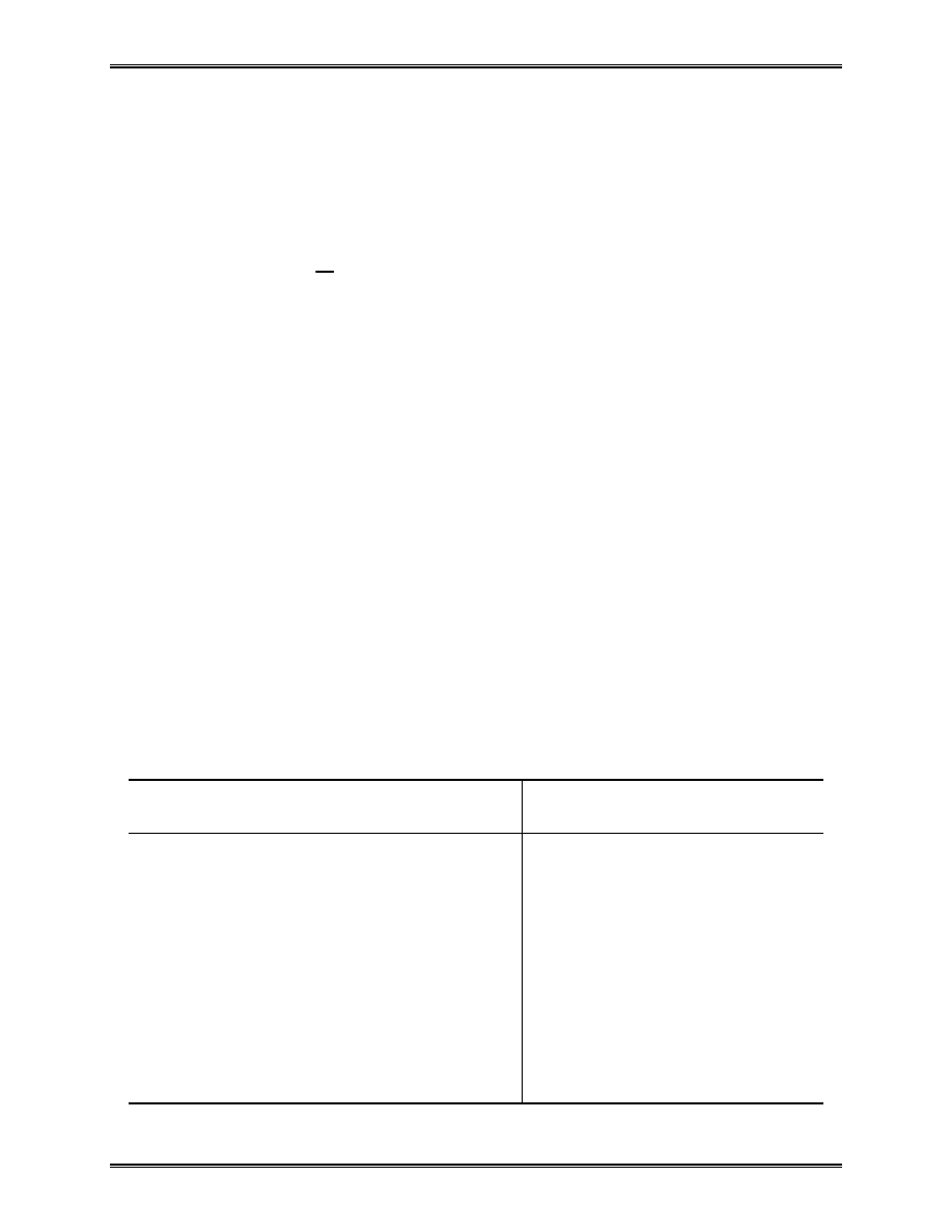
Lecture Notes: Introduction to Finite Element Method Chapter 7. Structural Vibration and Dynamics
© 1999 Yijun Liu, University of Cincinnati
175
B. Modal Method
First, do the transformation of the dynamic equations using
the modal matrix before the time marching:
),
(
2
,
)
(
1
t
p
z
z
z
t
z
i
i
i
i
i
i
i
m
i
i
i
=
+
+
Φ
=
=
∑
=
ω
ω
ξ
&
&&
z
u
u
i = 1,2,
⋅⋅⋅
, m.
Then, solve the uncoupled equations using an integration
method. Can use, e.g., 10%, of the total modes (m= n/10).
•
Uncoupled system,
•
Fewer equations,
•
No inverse of matrices,
•
More efficient for large problems.
Comparisons of the Methods
Direct Methods
Modal Method
•
Small model
•
More accurate (with small
∆
t)
•
Single loading
•
Shock loading
•
…
•
Large model
•
Higher modes ignored
•
Multiple loading
•
Periodic loading
•
…

Lecture Notes: Introduction to Finite Element Method Chapter 7. Structural Vibration and Dynamics
© 1999 Yijun Liu, University of Cincinnati
176
Cautions in Dynamic Analysis
•
Symmetry: It should not be used in the dynamic analysis
(normal modes, etc.) because symmetric structures can
have antisymmetric modes.
•
Mechanism, rigid body motion means
ω
= 0. Can use
this to check FEA models to see if they are properly
connected and/or supported.
•
Input for FEA: loading F(t) or F(
ω
) can be very
complicated in real applications and often needs to be
filtered first before used as input for FEA.
Examples
Impact, drop test, etc.
Document Outline
- Chapt_01_Lect01.pdf
- Chapt_01_Lect02.pdf
- Chapt_01_Lect03.pdf
- Chapt_01_Lect04.pdf
- Chapt_02_Lect01.pdf
- Chapt_02_Lect02.pdf
- Chapt_02_Lect03.pdf
- Chapt_02_Lect04.pdf
- Chapt_02_Lect05.pdf
- Chapt_02_Lect06.pdf
- Chapt_02_Lect07.pdf
- Chapt_03_Lect01.pdf
- Chapt_03_Lect02.pdf
- Chapt_03_Lect03.pdf
- Chapt_03_Lect04.pdf
- Chapt_04_Lect01.pdf
- Chapt_04_Lect02.pdf
- Chapt_04_Lect03.pdf
- Chapt_05_Lect01.pdf
- Chapt_05_Lect02.pdf
- Chapt_06_Lect01.pdf
- Chapt_06_Lect02.pdf
- Chapt_06_Lect03.pdf
- Chapt_07_Lect01.pdf
- Chapt_07_Lect02.pdf
- Chapt_07_Lect03.pdf
- Chapt_07_Lect04.pdf
Wyszukiwarka
Podobne podstrony:
FINITE ELEMENT METHOD II 09 intro
FINITE ELEMENT METHOD II 09 intro
Fascia in the Abdominal Wall to the Thigh KT method
9 Finite Element Method using ProENGINEER and ANSYS
Intro to the Arduino
The Beginning of the Monte Carlo Method [jnl article] N Metropolis (1987) WW
Elementary Number Theory Notes D Santos (2004) WW
Functional Analysis [lecture notes] D Arnold (1997) WW
Intro to Braided Geometry & Q Minkowski Space [jnl article] S Majid (1994) WW
8 Intro to lg socio1 LECTURE2014
4 Intro to lg morph LECTURE2014
12 Intro to origins of lg LECTURE2014
Butterworth Finite element analysis of Structural Steelwork Beam to Column Bolted Connections (2)
3 Intro to lg phonol LECTURE201 Nieznany
więcej podobnych podstron