
3
Basic Process Calculations
and Simulations in Drying
Zdzisław Pakowski and Arun S. Mujumdar
CONTENTS
General Rules for a Dryer Model Formulation....................................................................................... 55
3.4.1
ß
2006 by Taylor & Francis Group, LLC.

Nomenclature ................................................................................................................................................... 78
References ........................................................................................................................................................ 79
3.1 INTRODUCTION
Since the publication of the first and second editions of
this handbook, we have been witnessing a revolution in
methods of engineering calculations. Computer tools
have become easily available and have replaced the old
graphical methods. An entirely new discipline of com-
puter-aided process design (CAPD) has emerged.
Today even simple problems are solved using dedi-
cated computer software. The same is not necessarily
true for drying calculations; dedicated software for this
process is still scarce. However, general computing
tools including Excel, Mathcad, MATLAB, and
Mathematica are easily available in any engineering
company. Bearing this in mind, we have decided to
present here a more computer-oriented calculation
methodology and simulation methods than to rely on
old graphical and shortcut methods. This does not
mean that the computer will relieve one from thinking.
In this respect, the old simple methods and rules of
thumb are still valid and provide a simple common-
sense tool for verifying computer-generated results.
3.2 OBJECTIVES
Before going into details of process calculations we
need to determine when such calculations are neces-
sary in industrial practice. The following typical cases
can be distinguished:
.
Design—(a) selection of a suitable dryer type
and size for a given product to optimize the
capital and operating costs within the range of
limits imposed—this case is often termed pro-
cess synthesis in CAPD; (b) specification of all
process parameters and dimensioning of a
selected dryer type so the set of design param-
eters or assumptions is fulfilled—this is the com-
mon design problem.
.
Simulation—for a given dryer, calculation of
dryer performance including all inputs and out-
puts, internal distributions, and their time de-
pendence.
.
Optimization—in design and simulation an op-
timum for the specified set of parameters is
sought. The objective function can be formu-
lated in terms of economic, quality, or other
factors, and restrictions may be imposed on
ranges of parameters allowed.
.
Process control—for a given dryer and a speci-
fied vector of input and control parameters the
output parameters at a given instance are
sought. This is a special case when not only the
accuracy of the obtained results but the required
computation time is equally important. Al-
though drying is not always a rapid process, in
general for real-time control, calculations need
to provide an answer almost instantly. This usu-
ally requires a dedicated set of computational
tools like neural network models.
In all of the above methods we need a model of the
process as the core of our computational problem. A
model is a set of equations connecting all process
parameters and a set of constraints in the form of
inequalities describing adequately the behavior of the
system. When all process parameters are determined
with a probability equal to 1 we have a deterministic
model, otherwise the model is a stochastic one.
In the following sections we show how to construct
a suitable model of the process and how to solve it for a
given case. We will show only deterministic models of
convective drying. Models beyond this range are im-
portant but relatively less frequent in practice.
In our analysis we will consider each phase as a
continuum unless stated otherwise. In fact, elaborate
models exist describing aerodynamics of flow of gas and
granular solid mixture where phases are considered
noncontinuous (e.g., bubbling bed model of fluid bed,
two-phase model for pneumatic conveying, etc.).
3.3 BASIC CLASSES OF MODELS
AND GENERIC DRYER TYPES
Two classes of processes are encountered in practice:
steady state and unsteady state (batch). The differ-
ence can easily be seen in the form of general balance
equation of a given entity for a specific volume of
space (e.g., the dryer or a single phase contained in it):
Inputs
outputs ¼ accumulation
(3:1)
ß
2006 by Taylor & Francis Group, LLC.
For inst ance, for mass flow of mois ture in a solid
phase being dried (in kg/s) this equati on reads:
W
S
X
1
W
S
X
2
w
D
A
¼ m
S
dX
dt
(3 : 2)
In steady -state proc esses, as in all continuou sly ope r-
ated dryers , the accumul ation term van ishes and the
balance e quation assum es the form of an algebr aic
equati on. W hen the pro cess is of batch type or when a
continuous process is be ing started up or shut down,
the accumul ation term is nonzero an d the balance
equati on becomes an ord inary different ial equ ation
(ODE) with respect to time.
, we have assum ed that
only the inpu t an d output pa rameters coun t. Inde ed,
when the volume unde r con siderati on is perfec tly
mixed , all pha ses inside this volume will have the
same pr operty as that at the output. This is the prin-
ciple of a lumped pa rameter model (LPM).
If a pr operty varies c ontinuousl y along the flow
direction (in one dimens ion for sim plicity), the bal-
ance equatio n can only be writt en for a different ial
space elemen t. Here Equat ion 3.2 will now read
W
S
X
W
S
X
þ
@ X
@ l
dl
w
D
dA
¼ dm
S
@ X
@t
(3 : 3)
or, afte r su bstituting dA
¼ a
V
Sdl and dm
S
¼ (1 «)
r
S
S d l, we obtain
W
S
@ X
@ l
w
D
a
V
S
¼ (1 «) r
S
S
@ X
@t
(3 : 4)
As we can see for this case, which we call a dist ributed
parame ter mod el (DPM) , in steady state (in the one -
dimens ional case) the model beco mes an ODE wi th
respect to space coordinat e, and in uns teady state it
becomes a partial different ial eq uation (PDE). Thi s
has a far-reachi ng influen ce on methods of solvin g the
model. A corres pondi ng equati on will have to be
written for y et another phase (gaseo us), and the equ a-
tions will be co upled by the drying rate exp ression.
Befo re star ting with constru cting and solvin g a
specific dryer mod el it is reco mmended to class ify
the methods , so typic al cases c an easily be identifie d.
We will classify typic al cases when a soli d is co ntacted
with a he at carri er. Three facto rs will be co nsidered :
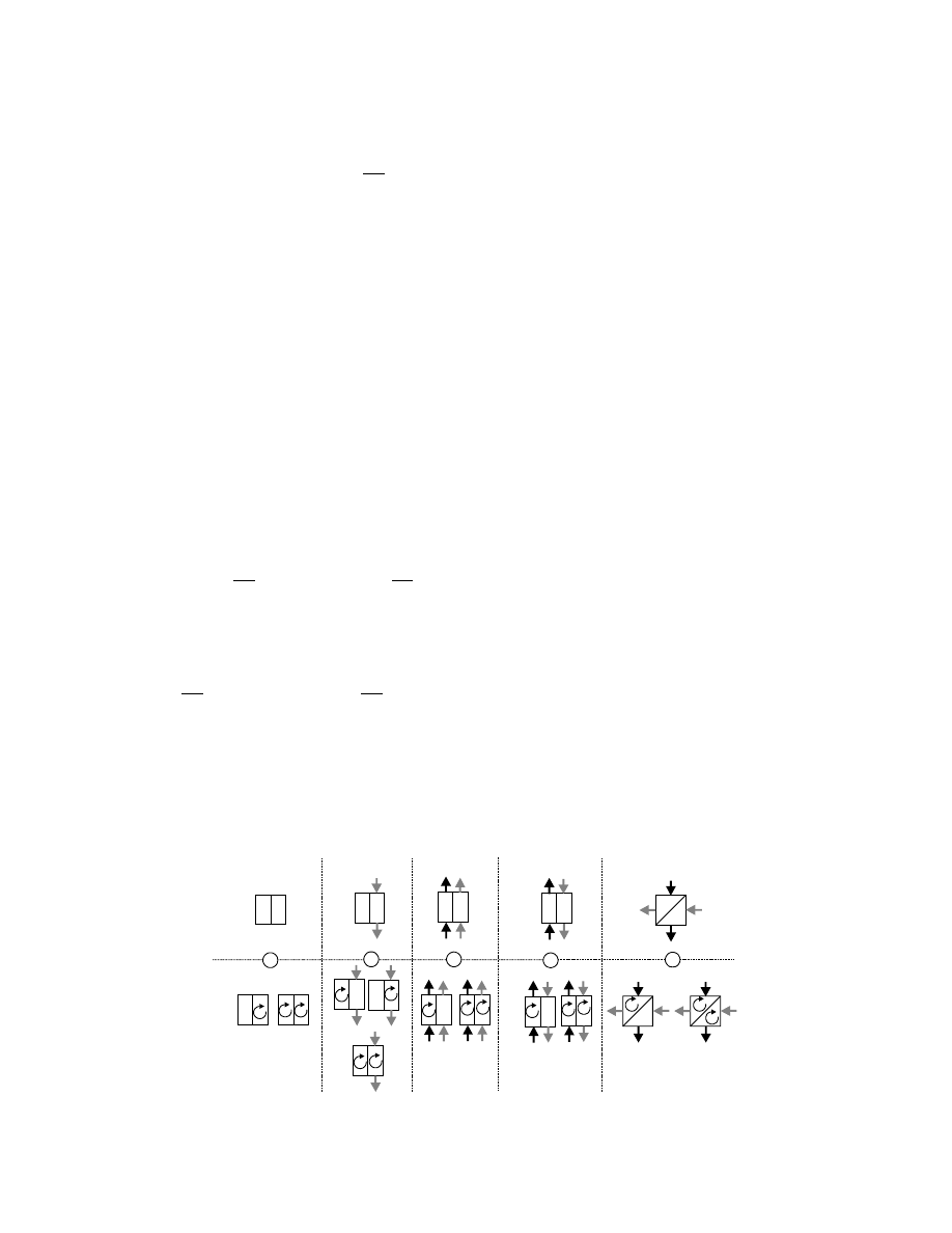
1. Operation type—we will co nsider eithe r batch
or co ntinuous process wi th respect to given
phase.
2. Flow g eometry type—w e will consider only
parallel flow, cocurrent , countercur rent, and
cross-flow cases.
3. Flow type—w e will con sider two lim iting cases,
either plug flow or perfectly mixe d flow.
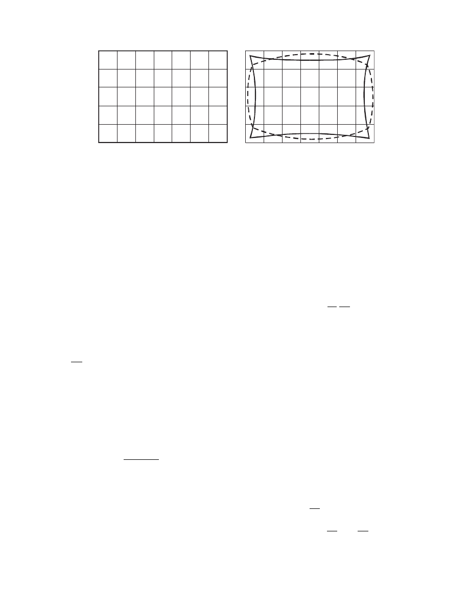
These three assum ptions for two pha ses present resul t
in 1 6 generic cases as sho wn in Figure 3.1. Before
constructing a model it is de sirable to identi fy the
class to whi ch it be longs so that writing appropriate
model equations is facilitated.
Dryers of type 1 do not exist in industry; there-
fore, dryers of type 2 are usually called batch dryers as
is done in this text. An additional term—semicontin-
uous —will be us ed for dry ers descri bed in
.
Their principle of operation is different from any of
the types shown in Figure 3.1.
3.4 GENERAL RULES FOR A DRYER MODEL
FORMULATION
When trying to derive a model of a dryer we first have to
identify a volume of space that will represent a dryer.
Batch
Semibatch
Continuous
countercurrent
Continuous
cocurrent
Continuous
cross-flow
No mixing
With ideal mixing of
one or two phases
a
a
a
a
a
b
b
b
b
b
c
c
c
c
c
d
1
2
4
5
3
FIGURE 3.1 Generic types of dryers.
ß
2006 by Taylor & Francis Group, LLC.

If a dryer or a whol e system is composed of many such
volume s, a separat e submod el will have to be built for
each vo lume and the mod els co nnected toget her by
streams e xchanged between them. Each stre am enter-
ing the volume must be identified wi th parame ters .
Basical ly for syst ems unde r c onstant pressur e it is
enough to describe e ach stream by the na me of the
compon ent (humi d gas, wet solid, conden sate, etc.),
its flowra te, moisture content , and tempe ratur e. All
heat an d other energy fluxe s must also be identified .
The followi ng five parts of a determ inistic mo del
can usually be dist inguishe d:
1. Balance equati ons—the y repres ent Natur e’s
laws of con servation and can be wri tten in
the form of
energy).
2. Constitu tive e quations (also called kinetic
equatio ns)—they conn ect fluxe s in the syst em
to respect ive drivi ng forces.
3. Equilib rium relationshi ps—neces sary if a pha se
bounda ry exist s somew here in the system.
4. Property equ ations—som e propert ies c an be
consider ed constant but, for exampl e, satura ted
water vap or pre ssure is strong ly dependen t on
temperatur e even in a narrow tempe rature
range.
5. Geometri c relationsh ips—they a re usually ne -
cessary to co nvert flowra tes present in balance
equatio ns to flux es present in consti tutive eq ua-
tions. Bas ically they include flow cross-sect ion,
specific area of phase contact , etc.
Typical form ulation of ba sic mod el eq uations will be
summ arized late r.
3.4.1 M
ASS AND
E
NERGY
B
ALANCES
Input–out put balance equ ations for a typical case of
convecti ve drying and LPM assum e the foll owing
form:
3.4.1.1 Mass Balances
Solid pha se:
W
S
X
1
W
S
X
2
w
Dm
A
¼ m
S
d X
dt
(3 : 5)
Gas pha se:
W
B
Y
1
W
B
Y
2
þ w
Dm
A
¼ m
B
dY
dt
(3 : 6)
3.4.1.2 Energy balances
Solid pha se:
W
S
i
m1
W
S
i
m2
þ (S q
m
w
Dm
h
A
)A
¼ m
S
di
m
dt
(3 : 7)
Gas pha se:
W
B
i
g1
W
B
i
g2
( Sq
m
w
Dm
h
A
)A
¼ m
B
d i
g
dt
(3 : 8)
In the above eq uations S q
m
an d w
Dm
are a sum of mean
interfaci al heat flux es and a drying rate, respectivel y.
Accum ulation in the gas phase ca n almos t alw ays be
neglected ev en in a batch process as smal l co mpared to
accumul ation in the soli d phase. In a continuous pro -
cess the accu mulation in solid pha se will also be
neglected .
In the case of DPMs for a given pha se the balance
equati on for prop erty G reads:
div [G
u] div[ D grad G] b a
V
DG
G
@G
@t
¼ 0
(3: 9)
where the LH S terms are, respectivel y (from the left):
convecti ve term, diffusion (or axial disper sion) term ,
interfaci al term, source or sink (prod uction or de-
struction) term, an d accumul ation term .
Thi s eq uation can now be writt en for a single pha se
for the case of mass an d energy transfer in the foll owing
way:
div[ r X
u] div[ D grad( r X ) ] k
X
a
V
DX
@r X
@t
¼ 0
(3 : 10)
div[ r c
m
T
u] div
l
r c
m
grad( r c
m
T )
aa
V
DT
þ q
ex
@rc
m
T
@t
¼ 0
(3:11)
Note that density here is related to the whole volume
of the phase: e.g., for solid phase composed of granu-
lar material it will be equal to r
m
(1
«). Moreover,
the interfacial term is expressed here as k
X
a
V
DX
for
consistency, although it is expressed as k
Y
a
V
DY
else-
where (
Now, consider a one-dimensional parallel flow of
two phases either in co- or countercurrent flow, ex-
changing mass and heat with each other. Neglecting
diffusional (or dispersion) terms, in steady state the
balance equations become
ß
2006 by Taylor & Francis Group, LLC.

W
S
dX
dl
¼ w
D
a
V
S (3 : 12)
W
B
d Y
dl
¼ w
D
a
V
S (3 : 13)
W
S
d i
m
dl
¼ ( q w
D
h
Av
) a
V
S (3 : 14)
W
B
di
g
dl
¼ ( q w
D
h
Av
) a
V
S (3 : 15)
where the LHSs of Equat ion 3.13 and Equat ion 3.15
carry the positive sign for cocurrent and the negative
sign for cou ntercurren t ope ration. Both heat and
mass fluxes, q and w
D
, are ca lculated from the con sti-
tutive equ ations as explai ned in the follo wing sectio n.
Havin g in mind that
di
g
dl
¼ ( c
B
þ c
A
Y )
dt
g
dl
þ ( c
A
t
g
þ D h
v0
)
dY
dl
(3 : 16)
and that enthal py of steam eman ating from the solid
is
h
Av
¼ c
A
t
m
þ Dh
v0
(3 : 17)
we can now rewrite (Eq uation 3.12 throu gh Equation
3.15) in a more con venient worki ng version
d X
d l
¼
S
W
S
w
D
a
V
(3 : 18)
d t
m
dl
¼
S
W
S
a
V
c
S
þ c
Al
X
[ q
þ w
D
( (c
Al
c
A
)t
m
Dh
v0
)]
(3 : 19)
d Y
dl
¼
1
x
S
W
B
w
D
a
V
(3 : 20)
dt
g
d l
¼
1
x
S
W
B
a
V
c
B
þ c
A
Y
[ q
þ w
D
c
A
( t
g
t
m
)] (3 : 21)
where x is 1 for cocurrent an d
1 for co untercur rent
operati on.
For a monoli thic soli d phase conv ective and inter -
facial terms disappea r and in uns teady stat e, for the
one-dim ensional case, the eq uations beco me
D
eff
@
2
X
@ x
2
¼
@ X
@t
(3 : 22)
l
@
2
t
m
@ x
2
¼ c
p
r
m
@ t
@t
(3 : 23)
These equati ons are named Fick ’s law and Fourier’ s
law, respect ively, and can be solved with suita ble
bounda ry and initial condition s. Li terature on solving
these eq uations is ab undan t, and for diff usion a clas-
sic work is that of Crank (1975) . It is wort h mentio n-
ing that, in view of irreversi ble thermod ynamics, mass
flux is also due to therm odiffu sion and barod iffusion.
Formula tion of Equation 3.22 an d Equation 3.23
contai ning terms of therm odiffu sion was favore d by
Luikov (1966) .
3.4.2 C
ONSTITUTIVE
E
QUATIONS
They are ne cessary to estimat e eithe r the local non-
convecti ve flux es caused by co nduction of heat or
diffusion of mois ture or the inter facial fluxes ex-
changed eithe r betw een two phases or through syst em
bounda ries (e.g ., heat losse s throu gh a wall) . The first
are usu ally express ed as
q
¼ l
dt
dl
(3 : 24)
j
¼ r D
eff
dX
dl
(3 : 25)
and they are alrea dy incorpora ted in the balance
equati ons (3.22 and 3.23). The interfaci al flux equ a-
tions assum e the foll owing form :
q
¼ a( t
g
t
m
)
(3:26)
w
D
¼ k
Y
f
(Y *
Y )
(3:27)
where f is
f
¼
M
A
=M
B
Y *
Y
ln 1
þ
Y *
Y
M
A
=M
B
þ Y
(3:28)
While the convective heat flux expression is straight-
forward, the expression for drying rate needs explan-
ation. The drying rate can be calculated from this
formula, when drying is controlled by gas-side resist-
ance. The driving force is then the difference between
absolute humidity at equilibrium with solid surface
and that of bulk gas. When solid surface is saturated
with moisture, the expression for Y* is identical to
; when solid surface co ntains bound
moisture, Y* will result from Equation 3.46 and a
sorption isotherm. This is in essence the so-called
equilibrium method of drying rate calculation.
When the drying rate is controlled by diffusion in
the solid phase (i.e., in the falling drying rate period),
the conditions at solid surface are difficult to find,
unless we are solving the DPM (Fick’s law or equiva-
lent) for the solid itself. Therefore, if the solid itself
has lumped parameters, its drying rate must be repre-
sented by an empirical expression. Two forms are
commonly used.
ß
2006 by Taylor & Francis Group, LLC.
3.4.2.1 Characteristic Drying Curve
In this approach the measured drying rate is repre-
sented as a function of the actual moisture content
(normalized) and the drying rate in the constant dry-
ing rate period:
w
D
¼ w
DI
f (F)
(3:29)
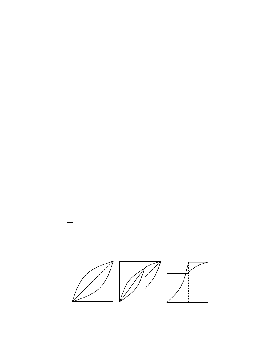
The f function can be represented in various forms to fit
the behavior of typical solids. The form proposed by
Langrish et al. (1991) is particularly useful. They split
the falling rate periods into two segments (as it often
occurs in practice) separated by F
B
. The equations are:
f
¼ F
a
c
B
for F # F
B
f
¼ F
a
for F > F
B
(3:30)
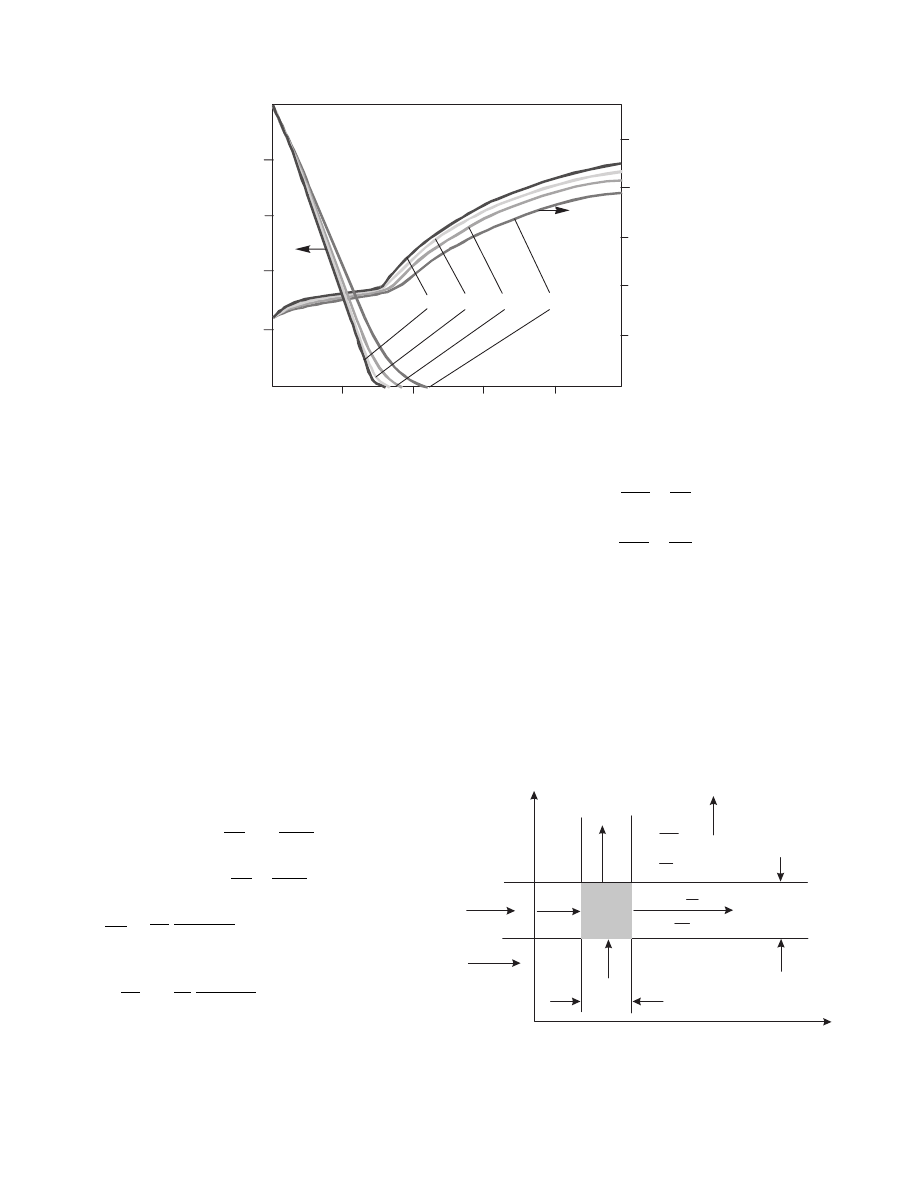
Figure 3.2 shows the form of a possible drying rate
curve using Equation 3.30.
Other such equations also exist in the literature
(e.g., Halstro¨m and Wimmerstedt, 1983; Nijdam and
Keey, 2000).
3.4.2.2 Kinetic Equation (e.g., Thin-Layer
Equations)
In agricultural sciences it is common to present drying
kinetics in the form of the following equation:
F
¼ f (t, process parameters)
(3:31)
The function f is often established theoretically, for
example, when using the drying model formulated by
Lewis (1921)
dX
dt
¼ k(X X *)
(3:32)
After integration one obtains
F
¼ exp (kt)
(3:33)
A similar equation can be obtained by solving Fick’s
equation in spherical geometry:
F
¼
6
p
2
X
1
n
¼1
1
n
2
exp
n
2
p
2
D
eff
R
2
t
(3:34)
By truncating the RHS side one obtains
F
¼
6
p
2
exp
p
2
D
eff
R
2
t
¼ a exp (kt)
(3:35)
This equation was empirically modified by Page
(1949), and is now known as the Page equation:
F
¼ exp (kt
n
)
(3:36)
A collection of such equations for popular agricul-
tural products is contained in Jayas et al. (1991).
Other process parameters such as air velocity, tem-
perature, and humidity are often incorporated into
these equations.
The volumetric drying rate, which is necessary in
balance equations, can be derived from the TLE in
the following way:
w
D
a
V
¼
m
S
A
a
V
dF
dt
(X
c
X *)
¼
m
S
V
dF
dt
(X
c
X *)
(3:37)
while
m
S
¼ V (1 «)r
S
(3:38)
and
w
D
a
V
¼ (1 «)r
S
(X
c
X *)
dF
dt
(3:39)
The drying rate ratio of CDC is then calculated as
Φ
B
f
c
<1
c
<1
a
<1
a
=1
a
>1
c
=1
c
>1
Φ
B
f
a
=
c<1
a
=
c
=1
a
=
c
>1
0
1
0
Φ
B
f
c
=
0
a
=
0
a
<1
1
FIGURE 3.2 The influence of parameters a and c of Equation 3.30 on CDC shape.
ß
2006 by Taylor & Francis Group, LLC.

f
¼
(1
«)r
S
(X
c
X *)
k
Y
f
( Y *
Y ) a
V
d F
dt
(3 : 40)
To be able to calcul ate the volume tric drying rate
from TLE, one needs to know the voidage « and
specific contact area a
V
in the dryer.
W hen dried soli ds are monoli thic or grain size is
overly large , the above lumped parame ter approxim a-
tions of drying rate woul d be una cceptable , in which
case a DPM repres ents the entire soli d phase. Such
models are shown in
.
3.4.3 A
UXILIARY
R
ELATIONSHIPS
3.4.3.1 Humid Gas Properties and Psychrometric
Calculations
The ability to perfor m psychro metric calcul ations
forms a basis on which all drying models are
built. One princi pal prob lem is how to determine the
solid tempe rature in the constant drying rate co ndi-
tions.
In psychrom etric calculati ons we co nsider therm o-
dynami cs of three pha ses: inert gas pha se, mois ture
vapor phase, and mois ture liquid pha se. Two gaseou s
phases form a solution (mixtur e) call ed humid gas. To
determ ine the degree of co mplex ity of our approach we
will make the follo wing assum ptions :
.
Inert gas componen t is insol uble in the liquid
phase
.
Gaseous phase be havior is close to ideal gas;
this limits our total pressur e ran ge to less than
2 bar
.
Liquid phase is incompr essi ble
.
Comp onents of both phases do not chemi cally
react with thems elves
Before writi ng the psyc hrometric relat ionship s we
will first present the ne cessary approxim ating equ a-
tions to descri be phy sical propert ies of syst em com-
ponen ts.
Depe ndence of satur ated vapor pressure on tem-
peratur e (e.g ., Antoin e eq uation):
ln p
s
¼ A
B
C
þ t
(3 : 41)
Dependen ce of late nt heat of vaporiz ation on tem-
peratur e (e.g ., Watson equati on):
Dh
v
¼ H ( t t
ref
)
n
(3 : 42)
Dependen ce of specific heat on temperatur e for vapo r
phase—polynomial form:
c
A
¼ c
A0
þ c
A1
t
þ c
A2
t
2
þ c
A3
t
3
(3:43)
Dependence of specific heat on temperature for liquid
phase—polynomial form:
c
Al
¼ c
Al0
þ c
Al1
t
þ c
Al2
t
2
þ c
Al3
t
3
(3:44)
Table 3.1 contains coefficients of the above listed
propert y eq uations for selec ted liqui ds and
for gases. These data can be found in specialized
books (e.g., Reid et al., 1987; Yaws, 1999) and com-
puterized data banks for other liquids and gases.
TABLE 3.1
Coefficients of Approximating Equations for Properties of Selected Liquids
Property
Water
Ethanol
Isopropanol
Toluene
Molar mass, kg/kmol
M
A
18.01
46.069
60.096
92.141
Saturated vapor pressure, kPa
A
16.376953
16.664044
18.428032
13.998714
B
3878.8223
3667.7049
4628.9558
3096.52
C
229.861
226.1864
252.636
219.48
Heat of vaporization, kJ/kg
H
352.58
110.17
104.358
47.409
t
ref
374.14
243.1
235.14
318.8
n
0.33052
0.4
0.371331
0.38
Specific heat of vapor, kJ/(kg K)
c
A0
1.883
0.02174
0.04636
0.4244
c
A1
10
3
0.16737
5.662
5.95837
6.2933
c
A2
10
6
0.84386
3.4616
3.54923
3.9623
c
A3
10
9
0.26966
0.8613
16.3354
0.93604
Specific heat of liquid, kJ/(kg K)
c
Al0
2.822232
1.4661
5.58272
0.61169
c
Al1
10
2
1.182771
4.0052
4.6261
1.9192
c
Al2
10
4
0.350477
1.5863
1.701
0.56354
c
Al3
10
8
3.60107
22.873
16.3354
5.9661
ß
2006 by Taylor & Francis Group, LLC.

3.4.3.2 Relations between Absolute Humidity,
Relative Humidity, Temperature,
and Enthalpy of Humid Gas
With the above assumptions and property equations
we can use Equation 3.45 through Equation 3.47 for
calculating these basic relationships (note that mois-
ture is described as component A and inert gas as
component B).
Definition of relative humidity w (we will use here
w
defined as decimal fraction instead of RH given in
percentage points):
w
(t)
¼ p=p
s
(t)
(3:45)
Relation between absolute and relative humidities:
Y
¼
M
A
M
B
wp
s
(t)
P
0
wp
s
(t)
(3:46)
Definition of enthalpy of humid gas (per unit mass of
dry gas):
i
g
¼ (c
A
Y
þ c
B
)t
þ Dh
v0
Y
(3:47)
Equation 3.46 and Equation 3.47 are sufficient to
find any two missing humid gas parameters from Y,
w
, t, i
g
, if the other two are given. These calculations
were traditionally done graphically using a psychro-
metric chart, but they are easy to perform numerically.
When solving these equations one must remember that
resulting Y for a given t must be lower than that at
saturation, otherwise the point will represent a fog
(supersaturated condition), not humid gas.
3.4.3.3 Calculations Involving Dew-Point
Temperature, Adiabatic-Saturation
Temperature, and Wet-Bulb Temperature
Dew-point temperature (DPT) is the temperature
reached by humid gas when it is cooled until it
becomes saturated (i.e., w
¼ 1). From Equation
3.46 we obtain
Y
s
¼
M
A
M
B
p
s
(t)
P
0
p
s
(t)
(3:48)
To find DPT when Y is known this equation must be
solved numerically. On the other hand, the inverse
problem is trivial and requires substituting DPT into
Equation 3.48.
Adiabatic-saturation temperature (AST) is the
temperature reached when adiabatically contacting
limited amounts of gas and liquid until equilibrium.
The suitable equation is
i
g
i
gs
,
AST
Y
Y
s
,
AST
¼ c
Al
t
AS
(3:49)
Wet-bulb temperature (WBT) is the one reached by a
small amount of liquid exposed to an infinite amount
of humid gas in steady state. The following are the
governing equations.
.
For water–air system, approximately
t
t
WB
Y
Y
s
,
WBT
¼
Dh
v
,
WBT
c
H
(3:50)
where
c
H
(t)
¼ c
A
(t)Y
þ c
B
(t)
(3:51)
Incidentally, this equation is equivalent to Equa-
tion 3.49 (see Treybal, 1980) for air and water
vapor system.
.
For other systems with higher Lewis numbers
the deviation of WBT from AST is noticeable
and can reach several degrees Celsius, thus caus-
ing serious errors in drying rate estimation. For
such systems the following equation is recom-
mended (Keey, 1978):
TABLE 3.2
Coefficients of Approximating Equations for Properties of Selected Gases
Property
Air
Nitrogen
CO
2
Molar mass, kg/kmol
M
B
28.9645
28.013
44.010
Specific heat of gas, kJ/(kg K)
c
B0
1.02287
1.0566764
0.48898
c
B1
10
3
0.5512
0.197286
1.46505
c
B2
10
6
0.181871
0.49471
0.94562
c
B3
10
9
0.05122
0.18832
0.23022
ß
2006 by Taylor & Francis Group, LLC.
t
t
WB
Y
Y
s
,
WBT
¼
Dh
v
,
WBT
c
H
Le
2=3
f
(3:52)
Typically in the wet-bulb calculations the fol-
lowing two situations are common:
.
One searches for humidity of gas of which both
dry- and wet-bulb temperatures are known: it is
enough to substitute relationships for Y
s
, Dh
v
,
and c
H
into Equation 3.52 and solve it for Y.
.
One searches for WBT once dry-bulb tempera-
ture and humidity are known: the same substi-
tutions are necessary but now one solves the
resulting equation for WBT.
The Lewis number
Le
¼
l
g
c
p
r
g
D
AB
(3:53)
is defined usually for conditions midway of the con-
vective boundary layer. Recent investigations (Berg
et al., 2002) indicate that Equation 3.52 needs correc-
tions to become applicable to systems of high WBT
approaching boiling point of liquid. However, for
common engineering applications it is usually suffi-
ciently accurate.
Over a narrow temperature range, e.g., for water–
air system between 0 and 1008C, to simplify calcula-
tions one can take constant specific heats equal to
c
A
¼ 1.91 and c
B
¼ 1.02 kJ/(kg K). In all calculations
involving enthalpy balances specific heats are averaged
between the reference and actual temperature.
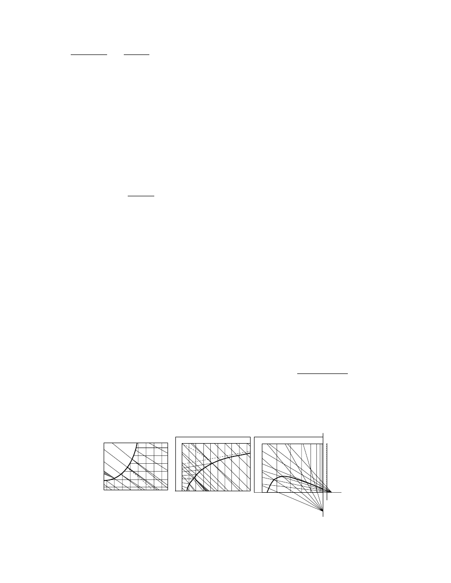
3.4.3.4 Construction of Psychrometric Charts
Construction of psychrometric charts by computer
methods is common. Three types of charts are most
popular: Grosvenor chart, Grosvenor (1907) (or the
psychrometric chart), Mollier chart, Mollier (1923)
(or enthalpy-humidity chart), and Salin chart (or
deformed enthalpy-humidity chart); these are shown
schematically in Figure 3.3.
Since the Grosvenor chart is plotted in undistorted
Cartesian coordinates, plotting procedures are simple.
Plotting methods are presented and charts of high ac-
curacy produced as explained in Shallcross (1994). Pro-
cedures for the Mollier chart plotting are explained in
Pakowski (1986) and Pakowski and Mujumdar (1987),
and those for the Salin chart in Soininen (1986).
It is worth stressing that computer-generated psy-
chrometric charts are used mainly as illustration ma-
terial for presenting computed results or experimental
data. They are now seldom used for graphical calcu-
lation of dryers.
3.4.3.5 Wet Solid Properties
Humid gas properties have been described together
with humid gas psychrometry. The pertinent data for
wet solid are presented below.
Sorption isotherms of the wet solid are, from the
point of view of model structure, equilibrium rela-
tionships, and are a property of the solid–liquid–
gas system. For the most common air–water system,
sorption isotherms are, however, traditionally consid-
ered as a solid property. Two forms of sorption iso-
therm equations exist—explicit and implicit:
w
*
¼ f (t,X )
(3:54)
X *
¼ f (t,a
w
)
(3:55)
where a
w
is the water activity and is practically
equivalent to w. The implicit equation, favored by
food and agricultural sciences, is of little use in
dryer calculations unless it can be converted to the
explicit form. In numerous cases it can be done ana-
lytically. For example, the GAB equation
X *
¼
aw
(1
bw)(1 þ cw)
(3:56)
can be solved analytically for w, and when the wrong
root is rejected, the only solution is
Mollier
i
i
i = const
t = const
t = const
i = const
i = const
t
Y
Y
Y
Grosvenor
j
= 1
j
= 1
j = 1
Salin
FIGURE 3.3 Schematics of the Grosvenor, Mollier, and Salin charts.
ß
2006 by Taylor & Francis Group, LLC.
w
*
¼
a
X
þ b c
þ
ffiffiffiffiffiffiffiffiffiffiffiffiffiffiffiffiffiffiffiffiffiffiffiffiffiffiffiffiffiffiffiffiffiffiffiffiffiffi
a
X
þ b c
2
þ 4bc
q
2bc
(3:57)
Numerous sorption isotherm equations (of approxi-
mately 80 available) cannot be analytically converted
to the explicit form. In this case they have to be solved
numerically for w* each time Y* is computed, i.e., at
every drying rate calculation. This slows down com-
putations considerably.
Sorptional capacity varies with temperature, and
the thermal effect associated with this phenomenon is
isosteric heat of sorption, which can be numerically
calculated using the Clausius–Clapeyron equation
Dh
s
¼
R
M
A
d ln w
d(1=T)
X
¼ const
(3:58)
If the sorption isotherm is temperature-independent
the heat of sorption is zero; therefore a number of
sorption isotherm equations used in agricultural sci-
ences are useless from the point of view of dryer
calculations unless drying is isothermal. It is note-
worthy that in the model equations derived in this
section the heat of sorption is neglected, but it can
easily be added by introducing Equation 3.59 for the
solid enthalpy in energy balances of the solid phase.
Wet solid enthalpy (per unit mass of dry solid) can
now be defined as
i
m
¼ (c
S
þ c
Al
X )t
m
Dh
s
X
(3:59)
The specific heat of dry solid c
S
is usually presented as
a polynomial dependence of temperature.
Diffusivity of moisture in the solid phase due to
various governing mechanisms will be here termed as
an effective diffusivity. It is often presented in the
Arrhenius form of dependence on temperature
D
eff
¼ D
0
exp
E
a
RT
(3:60)
However, it also depends on moisture content. Vari-
ous forms of dependence of D
eff
on t and X are
available (e.g., Marinos-Kouris and Maroulis, 1995).
3.4.4 P
ROPERTY
D
ATABASES
As in all process calculations, reliable property data
are essential (but not a guarantee) for obtaining sound
results. For drying, three separate databases are neces-
sary: for liquids (moisture), for gases, and for solids.
Data for gases and liquids are widespread and are
easily available in printed form (e.g., Yaws, 1999)
or in electronic version. Relatively good property
prediction methods exist (Reid et al., 1987). However,
when it comes to solids, we are almost always con-
fronted with a problem of availability of property
data. Only a few source books exist with data for
various products (Nikitina, 1968; Ginzburg and
Savina, 1982; Iglesias and Chirife, 1984). Some data
are available in this handbook also. However, numer-
ous data are spread over technical literature and re-
quire a thorough search. Finally, since solids are not
identical even if they represent the same product, it is
always recommended to measure all the required prop-
erties and fit them with necessary empirical equations.
The following solid property data are necessary
for an advanced dryer design:
.
Specific heat of bone-dry solid
.
Sorption isotherm
.
Diffusivity of water in solid phase
.
Shrinkage data
.
Particle size distribution for granular solids
3.5 GENERAL REMARKS ON SOLVING
MODELS
Whenever an attempt to solve a model is made, it is
necessary to calculate the degrees of freedom of the
model. It is defined as
N
D
¼ N
V
N
E
(3:61)
where N
V
is the number of variables and N
E
the num-
ber of independent equations. It applies also to models
that consist of algebraic, differential, integral, or other
forms of equations. Typically the number of variables
far exceeds the number of available equations. In this
case several selected variables must be made constants;
these selected variables are then called process vari-
ables. The model can be solved only when its degrees
of freedom are zero. It must be borne in mind that not
all vectors of process variables are valid or allow for a
successful solution of the model.
To solve models one needs appropriate tools.
They are either specialized for the specific dryer de-
sign or may have a form of universal mathematical
tools. In the second case, certain experience in hand-
ling these tools is necessary.
3.6 BASIC MODELS OF DRYERS
IN STEADY STATE
3.6.1 I
NPUT
–O
UTPUT
M
ODELS
Input–output models are suitable for the case when
both phases are perfectly mixed (cases 3c, 4c, and 5c
ß
2006 by Taylor & Francis Group, LLC.
), which almost never hap pens. On the
other ha nd, this mo del is very often used to repres ent
a case of unmixe d flows when there is lack of a DP M.
Input–out put modeli ng consis ts basica lly of balan-
cing all inputs and outp uts of a dryer and is often
perfor med to iden tify, for exampl e, heat losse s to the
surroundi ngs, calculate performan ce, and for dryer
audits in general .
For a steady-st ate dryer balanci ng can be made
for the whol e dryer only, so the system of
equati ons
W
S
( X
1
X
2
)
¼ W
B
( Y
2
Y
1
)
(3: 62)
W
S
( i
m2
i
m1
)
¼ W
B
( i
g1
i
g2
)
þ q
c
q
l
þ Dq
t
þ q
m
(3 : 63)
where sub scripts on heat fluxes indica te: c, indir ect
heat inp ut; l, heat losses; t, net he at carried in by
transp ort devices; and m, mechani cal en ergy input.
Let us assum e that all q, W
S
, W
B
, X
1
, i
m1
, Y
1
, i
g1
are
known as in a typic al design case. The remaining
variab les are X
2
, Y
2
, i
m2
, and i
g2
. Sin ce we have two
equati ons, the syst em ha s two degrees of freedom and
cannot be solved unless two other varia bles are set as
process pa rameters. In design we can assum e X
2
since
it is a design specifica tion, but then one ex tra param-
eter must be assum ed. This of co urse ca nnot be done
rationa lly, unless we are su re that the process runs in
constant drying rate pe riod—th en i
m2
can be calcu-
lated from WBT. Othe rwise, we must look for oth er
equati ons, whi ch could be the foll owing:
W
S
(X
1
X
2
)
¼ Va
V
k
Y
D Y
m
(3 : 64)
W
S
( i
m2
i
m1
)
¼ Va
V
(aDt
m
þ Sq
k
Y
DY
m
h
A
) (3 : 65)
Provided that we know all kineti c da ta, a
V
, k
Y
, and a,
these tw o equati ons carry onl y one new varia ble V
since tempe ratures can be derived from suitable
enthal pies. Provided that we know how to calcul ate
the average d drivi ng forces, the model now can be
solved and exit stream parame ters an d volume of the
dryer calcula ted. The success , howeve r, dep ends on
how well we can esti mate the average d drivi ng forces .
3.6.2 D
ISTRIBUTED
P
ARAMETER
M
ODELS
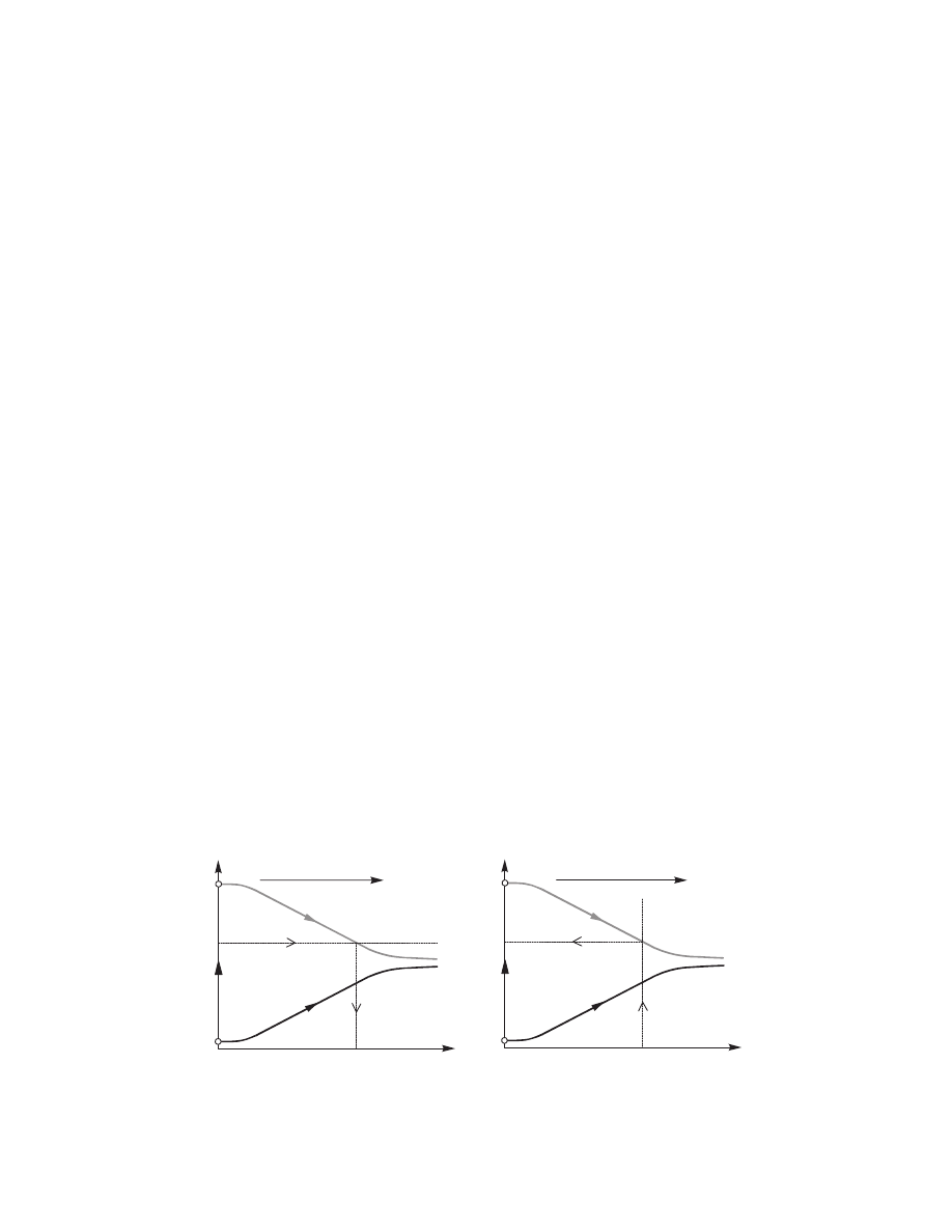
3.6.2.1 Cocurrent Flow
For cocurrent operatio n (case 3a in Figure 3.1) both
the case design and sim ulation are simple. The fou r
balance equ ations (
) supp lemented
by a suit able drying rate and heat flux equ ations
are solved starting at inlet end of the dr yer, where
all bounda ry conditio ns (i.e., all parame ters of incom-
ing streams) are defin ed. Thi s situ ation is shown in
Figure 3.4.
In the case of design the calcul ations are term in-
ated when the design parame ter, usually final mois -
ture con tent, is reached. Dis tance at this point is the
requir ed dryer length . In the case simu lation the cal-
culation s are terminat ed onc e the dryer lengt h is
reached.
Par ameters of both gas and solid pha se (repr e-
sented by gas in eq uilibrium with the so lid surfa ce)
can be plotted in a psychrom etric ch art as pro cess
paths. Thes e phase diagra ms (no timescal e is availab le
there) show schema tically how the pr ocess goes on.
To illustrate the case the mo del compo sed of
Equation 3.18 through Equation 3.21,
typical con ditions and the resul ts are sh own in
X
Y
X
des
L
L
des
Direction of integration
(a)
(b)
X
Y
L
L
X
1
Y
1
X
1
Y
1
X
2
Direction of integration
FIGURE 3.4 Schematic of design and simulation in cocurrent case: (a) design; (b) simulation. X
des
is the design value of final
moisture content.
ß
2006 by Taylor & Francis Group, LLC.
3.6.2.2 Countercurrent Flow
The situati on in countercur rent case (case 4a in
) design a nd sim ulation is shown in Fi gure 3.6.
In both cases we see that bounda ry conditio ns are
defined at oppos ite en ds of the integ ration domain.
It leads to the split boundar y value problem .
In design this prob lem can be avoided by using the
design parame ters for the solid specified at the exit
end. Then, by writin g input–out put balances ov er the
whole dryer, inlet parame ters of gas can easil y be
found (unles s local heat losses or other distribut ed
parame ter phe nomena need also be consider ed).
Howev er, in sim ulation the split bounda ry value
problem exist s and must be solved by a suit able nu-
merical method , e.g., the shooting met hod . Basical ly
the method consis ts of assum ing certain parame ters
for the exit ing gas stre am and perfor ming integ ration
starting at the so lid inlet end. If the gas parame ters at
the other en d conve rges to the known inlet gas
parame ters, the assum ption is sati sfactory; otherwis e,
a new assump tion is made. The process is repeat ed
under co ntrol of a suit able convergence co ntrol
method, e.g. , Wegst ein.
countercur rent c ase calcul ation for the same mate rial
as that used in Figu re 3.5.
0
20
40
60
80
% of dryer length
100
0.0
25.0
50.0
50.0
75.0
100.0
125.0
150.0
150.0
175.0
200.0
225.0
t
⬚C
0.0
10.0
20.0
30.0
40.0
50.0
60.0
70.0
80.0
0.0
0.0
0.0
0.0
20.0
20.0
40.0
60.0
80.0
100.0
100.0
120.0
140.0
160.0
180.0
200.0
200.0 220.0
40.0 60.0 80.0
g/kg
10.0
20.0
30.0
40.0
50.0
60.0
70.0
80.0
90.0
100.0
dryPAK v.3.6
dryPAK v.3.6
Calculated profile graph
for cocurrent contact of sand
containing water with air
Y, g/kg X, g/kg
⬚C
Continuous cocurrent contact of sand and water in air
20
30
40
50
60
70
80
90
100
t
m
t
g
y
x
250.0
300.0
350.0
400.0
450.0
kJ/kg
10
@101.325 kPa
FIGURE 3.5 Process paths and longitudinal distribution of parameters for cocurrent drying of sand in air.
X
Y
X
des
L
L
des
X
1
Y
1
Y
1
Direction of integration
X
Y
L
L
X
1
Y
1
Y
2
⬘
Y
2
X
2
Direction of integration
(a)
(b)
FIGURE 3.6 Schematic of design and simulation in cocurrent case: (a) design—split boundary value problem is avoided by
calculating Y
1
from the overall mass balance; (b) simulation—split boundary value problem cannot be avoided, broken line
shows an unsuccessful iteration, solid line shows a successful iteration—with Y
2
assumed the Y profile converged to Y
1
.
ß
2006 by Taylor & Francis Group, LLC.
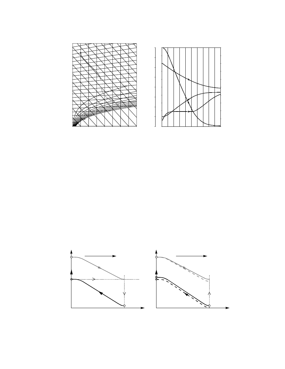
3.6.2.3 Cross-Flow
3.6.2.3.1 Solid Phase is One-Dimensional
This is a sim ple case corresp onding to case 5b of
. By assuming that the so lid phase is per-
fectly mixe d in the direction of gas flow, the solid
phase beco mes one -dimen sional. This situ ation oc -
curs with a co ntinuous plug-flow fluid be d dryer.
Schemat ic of an elem ent of the dr yer length wi th finite
thickne ss D l is sho wn in Figure 3.8.
The balance e quations for the solid pha se can be
parallel flow:
W
S
S
dX
dl
¼ w
D
a
V
(3 : 66)
W
S
S
di
m
d l
¼ ( q w
D
h
Av
) a
V
(3 : 67)
The analogo us eq uations for the gas phase are:
mass balance
1
S
dW
B
(Y
2
Y
1
)
dl
¼ w
D
a
V
(3 : 68)
energy balance
1
S
dW
B
( i
g2
i
g1
)
dl
¼ (q w
D
h
Av
) a
V
(3 : 69)
In the case of an eq uilibrium method of calculati on of
the dry ing rate the kineti c eq uations are:
w
D
¼ k
Y
D Y
m
(3 : 70)
q
¼ aDt
m
(3 : 71)
In other models (CDC an d TLE) the drying rate will
be modified as sh own in
Since the heat and mass coeffici ents can be defined
on the basis of eithe r the inlet drivi ng force or the
mean logari thmic driving force, DY
m
and D t
m
are
calculated respect ively as
DY
m
¼ (Y * Y
1
)
(3: 72)
0
0.0
0.0
0.0
10.0
10.0
10.0
20.0
20.0
20.0
30.0
30.0
30.0
40.0
40.0
40.0
50.0
50.0
50.0
60.0
60.0
60.0
70.0
70.0
70.0
80.0
80.0
80.0
90.0
90.0
Y, g/kg x, g/kg
100.0
110.0
0.0
0.0
25.0
50.0
75.0
100.0
125.0
150.0
175.0
200.0
20.0
40.0
60.0
80.0
100.0
120.0
140.0
160.0
180.0
200.0
220.0
225.0 250.0 275.0 300.0 325.0 350.0 375.0 400.0 425.0 450.0
10 20 30 40 50 60 70 80 90 100
% of dryer length
0.0
20.0
40.0
60.0
80.0
100.0
120.0
140.0
160.0
180.0
200.0
220.0
t, ⬚C
dryPAKv.3.6
g/kg
⬚C
dryPAK v.3.6
20
30
40
50
60
70
80
90
100
Calculated profile graph
for countercurrent contact of sand
containing water with air
Continuous countercurrent contact of sand and water in air
kJ/kg
@101.325 kPa
10
t
m
y
x
t
g
FIGURE 3.7 Process paths and longitudinal distribution of parameters for countercurrent drying of sand in air.
d
l
d
W
B
d
W
B
Y
1
Y
2
i
g
1
i
g2
W
S
X
W
S
i
m
X+ dl
i
m
+ d
l
d
X
d
l
d
i
m
d
l
_
_
__
FIGURE 3.8 Element of a cross-flow dryer.
ß
2006 by Taylor & Francis Group, LLC.
or
D Y
m
¼
Y
2
Y
1
ln
Y *
Y
1
Y *
Y
2
(3 : 73)
Dt
m
¼ (t
m
t
g1
)
(3: 74)
or
Dt
m
¼
t
g2
t
g1
ln
t
m
t
g2
t
m
t
g1
(3 : 75)
one need s
to assum e a unifor m dist ribution of gas over the
whole lengt h of the dryer, an d therefore
dW
B
dl
¼
W
B
L
(3 : 76)
When the algebr aic Equation 3.68 and Equat ion 3.69
are solved to obtain the exiting gas parame ters Y
2
and
i
g2
, one c an plug the LH S of these equati ons into
and
to obtain
dX
dl
¼
1
W
S
W
B
L
( Y
2
Y
1
)
(3: 77)
di
m
dl
¼
1
W
S
W
B
L
( i
g2
i
g1
)
(3: 78)
The followi ng equ ations can easil y be integrate d
starting at the soli ds inlet. In Figu re 3.9 sample pr o-
cess pa rameter profiles alon g the dryer are sho wn.
Cros s-flow drying in a plug-flow , continuou s fluid
bed is a case when axial disper sion of flow is often
consider ed. Let us briefly present a method of solving
this case. First, the governi ng ba lance equ ations for
the soli d pha se will have the followi ng form de rived
from
u
m
dX
dl
¼ E
m
d
2
X
dl
2
a
V
w
D
r
S
(1
«)
(3 : 79)
u
m
di
m
d l
¼ E
h
d
2
i
m
d l
2
þ
a
V
( q
w
D
h
Av
)
r
S
(1
«)
(3 : 80)
or
u
m
dt
m
dl
¼ E
h
d
2
i
m
dl
2
þ
a
V
r
S
(1
«)
1
c
S
þ c
Al
X
[ q þ ((c
Al
c
A
) t
m
D h
v0
)w
D
] (3 : 81)
where
u
m
¼
W
S
r
S
(1
«)
(3:82)
These equations are supplemented by equations for
w
D
and q according to Equation 3.70 and Equation
3.71. It is a common assumption that E
m
¼ E
h
,
because in fluid beds they result from longitudinal
mixing by rising bubbles. Boundary conditions
(BCs) assume the following form:
At l
¼ 0
X
¼ X
0
and
i
m
¼ i
m0
(3:83)
At l
¼ L
dX
dl
¼ 0
and
di
m
dl
¼ 0
(3:84)
0
10
0
0.2
0.4
0.6
Dryer length, m
X
, kg/kg
Y
*10, kg/kg
0
10
0
50
100
150
Dryer length, m
Temperature,
⬚C
t
WB
5
5
(a)
(b)
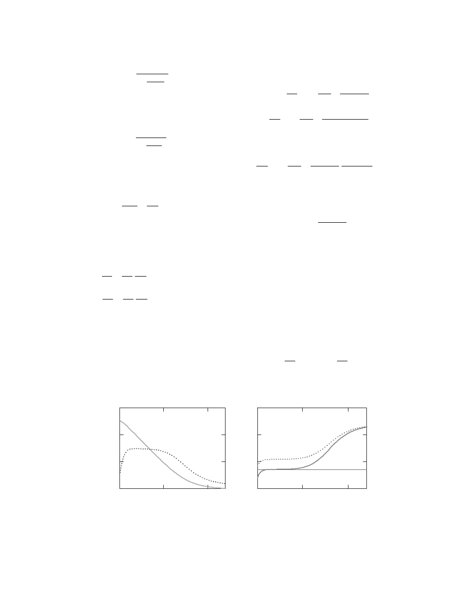
FIGURE 3.9 Longitudinal parameter distribution for a cross-flow dryer with one-dimensional solid flow. Drying of a
moderately hygroscopic solid: (a) material moisture content (solid line) and local exit air humidity (broken line): (b) material
temperature (solid line) and local exit air temperature (broken line). t
WB
is wetbulb temperature of the incoming air.
ß
2006 by Taylor & Francis Group, LLC.
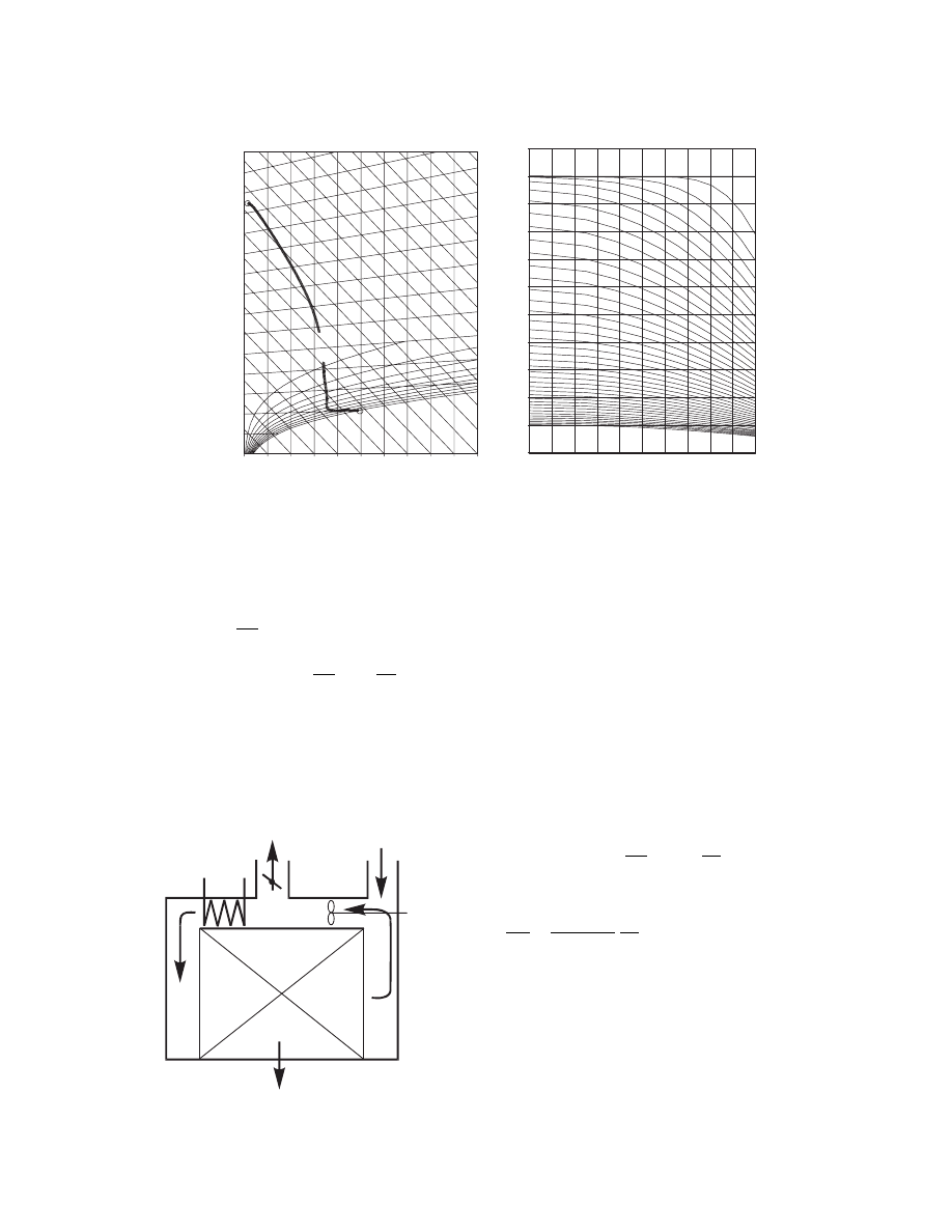
The secon d BC is due to Danck werts a nd has been used
for chemi cal reactor mo dels. This leads, of co urse, to a
split bounda ry value problem , whi ch needs to be
solved by an appropri ate numerica l techni que. The
resulting longit udinal profi les of solid moisture co n-
tent and tempe ratur e in a dryer for various Pec let
numbers ( Pe
¼ u
m
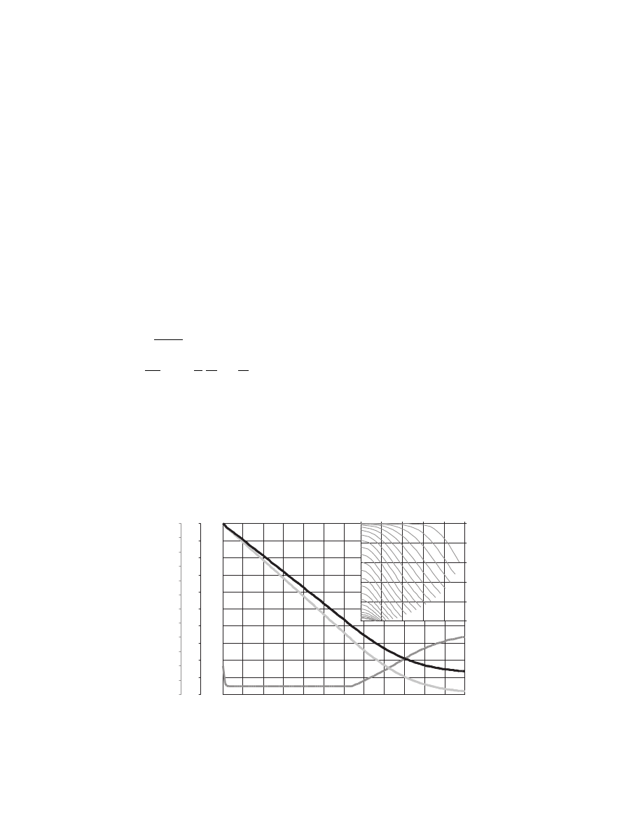
L/E ) are present ed in Figure 3.10.
As one can see, only at low Pe numbe rs, pro files
differ signi ficantl y. When Pe > 0.5, the flow may be
consider ed a plug-flow.
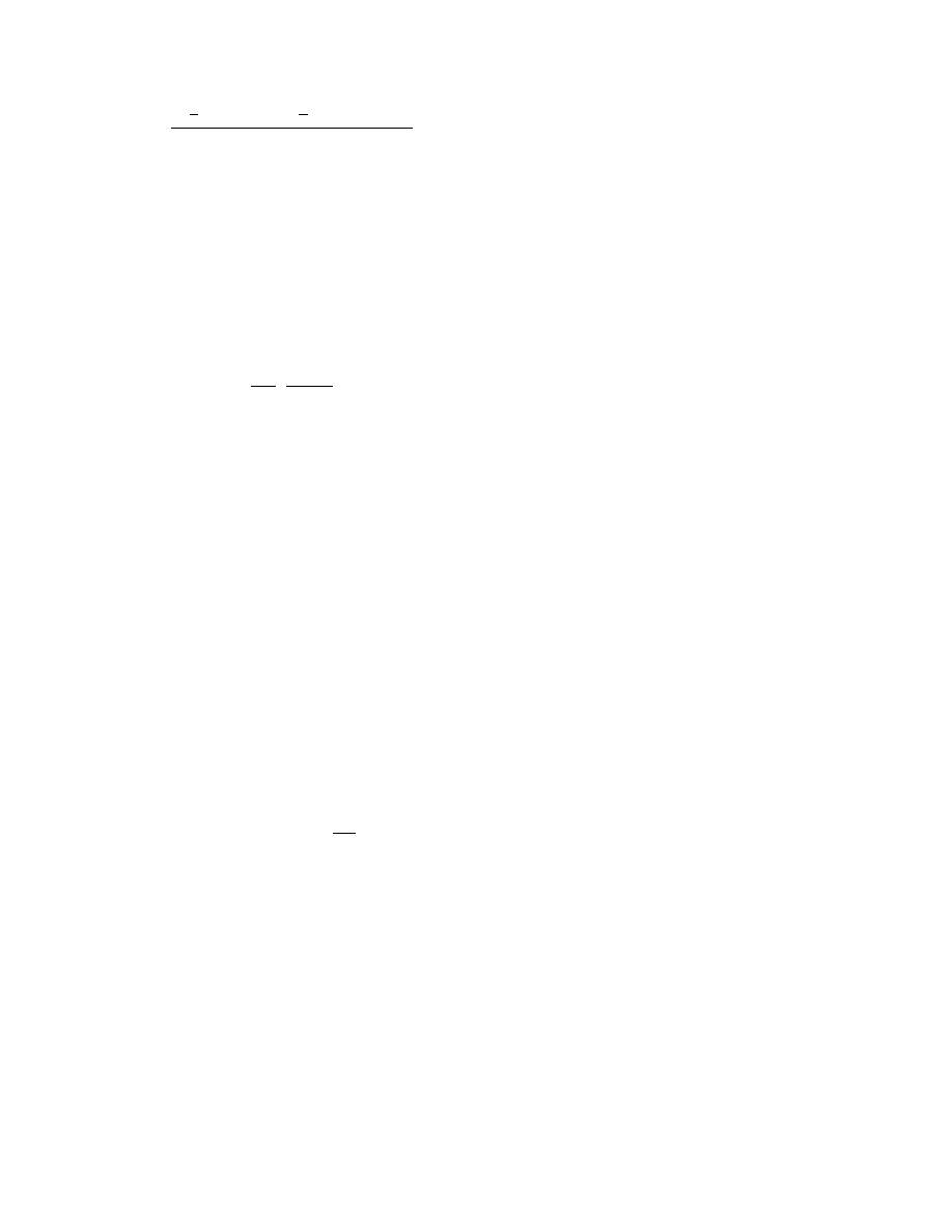
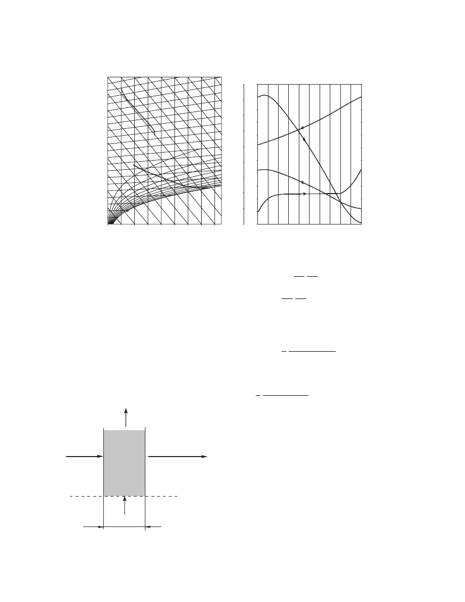
3.6.2.3.2 Solid Phase is Two-Dimensional
This case ha ppens when solid phase is not mixe d
but moves as a block. This situati on happ ens in
certain dryers for wet grains. The mod el must
be de rived for different ial bed eleme nt as shown in
Figure 3.11.
The model e quations are now:
dX
dl
¼
w
D
a
V
s
H
(3 : 85)
dY
d h
¼
w
D
a
V
s
L
(3 : 86)
dt
m
d l
¼
a
V
s
H
1
c
S
þ c
Al
X
[q (( c
A
c
Al
)t
m
þ Dh
v0
) w
D
]
(3 : 87)
dt
g
dh
¼
a
V
s
L
1
c
B
þ c
A
Y
[ q
þ c
A
(t
g
t
m
) w
D
]
(3: 88)
The symbols s
H
and s
L
are flow den sities pe r 1 m for
solid and gas mass flowra tes, respect ively, an d are
defined as follows :
s
H
¼
d W
S
dh
¼
W
S
H
(3 : 89)
s
L
¼
dW
B
dl
¼
W
B
L
(3 : 90)
The third term in these form ulatio ns app lies when
distribut ion of flow is uniform, otherwis e an adequ ate
distribut ion fun ction must be used. An ex emplary
model solut ion is shown in
. The solution
only presents the heat transfer case (cooling of granu-
lar solid with air), so mass transfer equations are
neglected.
0
0
0.2
0.4
0.6
0.8
0
0.5
1.0
1.5
2.0
2.5
t
m
/
t
WB
0.2
0.4
0.6
0.8
Φ
Pe = ∞ > Pe
3
>
Pe
2
>
Pe
1
I/L
FIGURE 3.10 Sample profiles of material moisture content and temperature for various Pe numbers.
d
W
S
d
W
S
(
t
m
+
dl
)
d
t
m
d
l
d
X
d
l
(
t
g
+
d
h
)
(
Y+ dh
)
d
t
g
d
h
d
Y
d
h
d
W
S
W
S
W
B
l
h
d
l
d
h
t
m
X
(
X + dl
)
d
W
B
t
g
Y
d
W
B
FIGURE 3.11 Schematic of a two-dimensional cross-flow
dryer.
ß
2006 by Taylor & Francis Group, LLC.
3.7 DISTRIBUTED PARAMETER MODELS
FOR THE SOLID
This case occu rs when dried soli ds are mono lithic or
have large grain size so that LPM for the drying rate
would be an una cceptabl e ap proximati on. To answ er
the que stion as to wheth er this case applies one has to
calcula te the Biot num ber for mass trans fer. It is
recomm ended to calculate it from
since various de finition s are foun d in the literat ure.
When Bi < 1, the case is exter nally control led and no
DPM for the soli d is requir ed.
3.7.1 ONE-DIMENSIONAL MODELS
3.7.1.1 N
ONSHRINKING
S
OLIDS
Assuming that mois ture diffusion takes place in one
direction only, i.e., in the direction normal to surface
for plate an d in radial direction for cyli nder and
sphere, and that no other way of mo isture transp ort
exists but diffusion, the followin g second Fick’s law
may be de rived
@ X
@t
¼
1
r
n
@
@ r
r
n
D
eff
(t
m
, X )
@ X
@ r
(3 : 91)
where n
¼ 0 for plate , 1 for cylin der, 2 for sph ere, and
r is current distan ce (radiu s) measur ed from the solid
center . This parame ter reaches a maxi mum value of
R, i.e., plate is 2R thick if dried at both sides.
Initially we assume that moisture content is uni-
formly distributed and the initial solid moisture con-
tent is X
0
. To solve Equation 3.91 one requires a set of
BCs. For high Bi numbers (Bi > 100) BC is called BC
of the first kind and assumes the following form at the
solid surface:
At r
¼ R
X
¼ X *(t,Y )
(3:92)
For moderate Bi numbers (1 < Bi < 100) it is known as
BC of the third kind and assumes the following form:
At r
¼ R
D
eff
r
m
@X
@r
i
¼ k
Y
[Y *(X ,t)
i
Y ]
(3:93)
where subscript i denotes the solid–gas interface. BC
of the second kind as known from calculus (constant
flux at the surface)
At r
¼ R
w
Di
¼ const
(3:94)
has little practical interest and can be incorporated in
BC of the third kind. Quite often (here as well),
therefore, BC of the third kind is named BC of the
second kind. Additionally, at the symmetry plane we
have
At r
¼ 0
@X
@r
¼ 0
(3:95)
When solving the Fick’s equation with constant dif-
fusivity it is recommended to convert it to a dimen-
sionless form. The following dimensionless variables
are introduced for this purpose:
F
¼
X
X *
X
c
X *
,
Fo
¼
D
eff 0
t
R
2
,
z
¼
r
R
(3:96)
In the nondimensional form Fick’s equation becomes
@X
@Fo
¼
1
z
n
@
@z
z
n
D
eff
D
eff 0
@F
@z
(3:97)
and the BCs assume the following form:
BC I BC II
at z
¼ 1,
F
¼ 0
@F
@z
i
þBi
*
D
F
¼ 0
(3:98)
at z
¼ 0,
@F
@z
¼ 0
@F
@r
¼ 0
(3:99)
0
0
5
5
10
10
20
20
40
60
80
100
15
15
20
t
g ,
t
m
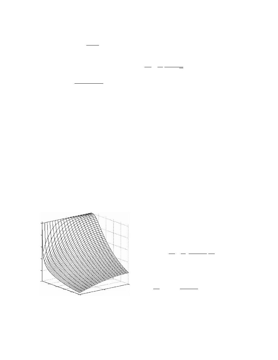
FIGURE 3.12 Solution of a two-dimensional cross-flow
dryer model for cooling of granular solid with hot air.
Solid flow enters through the front face of the cube, gas
flows from left to right. Upper surface, solid temperature;
lower surface, gas temperature.
ß
2006 by Taylor & Francis Group, LLC.
where
Bi
*
D
¼ m
XY
k
Y
fR
D
eff
r
m
(3 : 100)
is the modified Biot num ber in which m
XY
is a local
slope of equ ilibrium curve given by the foll owing
express ion:
m
XY
¼
Y *(X , t
m
)
i
Y
X
X *
(3 : 101)
The diffusional Biot numb er modified by the m
XY
factor sho uld be used for classificat ion of the cases
instead of Bi
D
¼ k
Y
R/( D
eff
r
m
) encoun tered in severa l
texts. Note that due to depen dence of D
eff
on X Bi ot
number can vary dur ing the course of drying, thu s
changing classificat ion of the prob lem.
Sin ce drying usuall y pro ceeds wi th varyi ng exter nal
conditi ons and variable diff usivity, analytical solu-
tions will be of littl e inter est. Instead we suggest us ing
a general-purp ose tool for solvi ng parabolic (
) and ellip tic PDE in one-dim ensional geomet ry
like the pdepe so lver of MATL AB. The resul t for Bi
*
D
¼ 5 obtaine d with this tool is shown in Figure 3.13.
The resul ts wer e obtaine d for isothermal conditio ns.
When conditio ns are nonisot hermal , a questi on aris es
as to wheth er it is necessa ry to sim ultaneo usly solve
Equation 3.22 and Equation 3.23. Since Bi ot num bers
for mass transfer far exceed those for heat trans fer,
usually the prob lem of heat transfer is pur ely exter nal,
and interna l profiles of tempe rature are almost flat.
This allow s one to use LPM for the energy ba lance.
Therefor e, to mo nitor the solid tempe ratur e it is
enough to supplem ent
ing energy balance equatio n:
dt
m
d t
¼
A
m
S
1
c
S
þ c
Al
X
[ q
þ ( (c
A
c
Al
) t
m
þ Dh
v0
) w
D
]
(3 : 102)
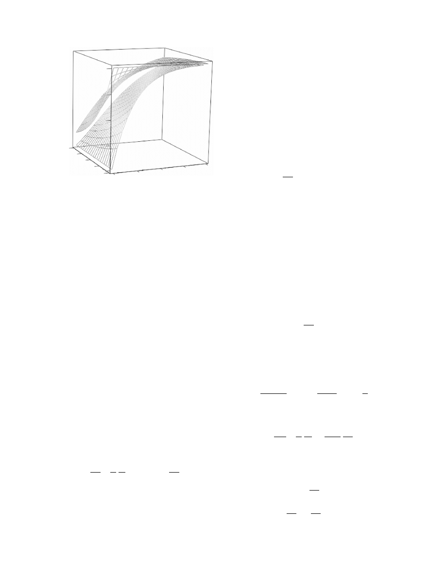
simulta neously, the pro blem beco mes stiff and re-
quires specia lize d solvers.
3.7.1.2 Shrinking Solids
3.7.1.2.1 Unrestrained Shrinkage
When solid s shrink vo lumetric ally (majori ty of food
products doe s), their volume is us ually related to
moisture content by the foll owing empir ical law:
V
¼ V
s
(1
þ sX )
(3: 103)
If one assumes that, for instance, a plate shrinks only
in the direct ion of its thickne ss, the follo wing rela-
tionsh ip may be deduc ed from the a bove equati on:
R
¼ R
s
(1
þ sX )
(3: 104)
where R is the actual plate thickn ess and R
s
is the
thickne ss of absolut ely dry plate .
In Euleri an coordinat es, shrinkin g causes an a d-
vective mass flux , which is difficult to ha ndle. By
changing the co ordinat e system to Lag rangia n, i.e.,
the one conn ected wi th dry mass basis, it is possible
to eliminat e this flux. This is the princi ple of a
method pro posed by Kechaou and Roq ues (1990) .
In Lagrang ian coordinat es
for one -
dimens ional shrinka ge of an infinite plate be comes:
@ X
@t
¼
@
@z
D
eff
(1
þ sX )
2
@ X
@z
(3 : 105)
All bounda ry and init ial condition s remain but the
BC of
@X
@z
z
¼R
S
¼
(1
þ sX )
2
r
S
D
eff
k
Y
(Y *
Y )
(3:106)
In Equation 3.105 and Equation 3.106, z is the
Lagrangian space coordinate, and it changes from 0
to R
s
. For the above case of one-dimensional shrink-
age the relationship between r and z is identical to
that in Equation 3.104:
1
1
1
0.8
0.8
0.6
0.6
0.4
0.4
0.2
0.2
0
0.5
x/L
Fo
0
Φ
FIGURE 3.13 Solution of the DPM isothermal drying
model of one-dimensional plate by pdepe solver of
MATLAB. Finite difference discretization by uniform
mesh both for space and time, Bi
*
D
¼ 5. Fo is dimensionless
time, x/L is dimensionless distance.
ß
2006 by Taylor & Francis Group, LLC.
r
¼ z (1 þ sX )
(3: 107)
The mo del was proved to work well for solids wi th
s > 1 (gel atin, polyacr ylam ide g el). An exemp lary
solution of this model for a shrinki ng gelatin film is
shown in Figure 3.14.
3.7.1.2.2 Restrained Shrinkage
For many mate rials shrinka ge accompan ying the
drying pr ocess may be opposed by the rigidit y of
the soli d skeleton or by viscous forces in liquid
phase a s it is co mpressed by sh rinking extern al
layers. This results in de velopm ent of stre ss within
the soli d. The developm ent of stress is inter esting
from the poin t of view of possible da mage of dr ied
produc t by deformati on or c racking . In or der to ac-
count for this, new eq uations have to be a dded to
Equation 3.10 and Equat ion 3.11. These are the bal-
ance of force eq uation an d liquid mois ture flow eq ua-
tion writt en as
G
r
2
U
þ
G
1
2n
r e ar p ¼ 0
(3: 108)
k
m
Al
r
2
p
¼
1
Q
@ p
@t
þ a
@ e
@t
(3 : 109)
where U is the deform ation matr ix, e is strain tensor
elemen t, and p is internal pressur e ( Q and a are
constant s). The eq uations were developed by Bi ot
and are explain ed in detai l by Hasat ani and Itaya
(1996). Equat ion 3.108 a nd Equat ion 3.109 can be
provided that a suita ble rheologica l mod el
of the soli d is known . The solution is almos t
always obtaine d by the finite elem ent method due to
inevitable deform ation of geomet ry. Solu tion of
such pro blems is complex an d requir es much more
computa tional power than any oth er problem in this
section.
3.7.2 T
WO
-
AND
T
HREE
-D
IMENSIONAL
M
ODELS
In fact some suppo sedly three-d imensional cases can
be co nverted to one -dimen sional by trans form ation
of the coordinat e syst em. This allows one to use a
finite diffe rence method , which is easy to program .
Lima et al. (2001) show how ovo id soli ds (e.g ., cereal
grains, silkworm cocoons) can be modeled by a one-
dimensional model. This even allows for uniform
shrinkage to be considered in the model. However,
in the case of two- and three-dimensional models
when shrinkage is not negligible, the finite difference
method can no longer be used. This is due to unavoid-
able deformation of corner elements, as shown in
.
The finite element methods have been used instead
for two- and three-dimensional shrinking solids (see
Perre and Turner, 1999, 2000). So far no commercial
software was proven to be able to handle drying
problems in this case and all reported simulations
were performed by programs individually written for
the purpose.
t
m
dryA
K
v
.3.6P
0
100 200 300 400 500 600 700 800 900 1000 1100 1200
Time, min
0.0
0.0
0.1
0.2
0.3
0.4
0.5
0.6
0.7
0.8
1.0
0.0
15
20
25
30
35
40
45
0.2
0.4
0.6
0.8
1.0
0.9
0.0
0.2
0.2
0.4
0.4
0.6
0.6
0.8
0.8
1.0
1.0
Φ,−
r/R,−
t
m
,
−
Φ,−
d,
−
Drying curve by Fickian diffusion: plate, BC II
with shrinkage for gelatine at 26.0
⬚C
d
FIGURE 3.14 Solution of a model of drying for a shrinking solid. Gelatin plate 3-mm thick, initial moisture content
6.55 kg/kg. Shrinkage coefficient s
¼ 1.36. Main plot shows dimensionless moisture content F, dimensionless thickness
d
¼ R/R
0
, solid temperature t
m
. Insert shows evolution of the internal profiles of F.
ß
2006 by Taylor & Francis Group, LLC.
3.7.3 S
IMULTANEOUS
S
OLVING
DPM
OF
S
OLIDS
AND
G
AS
P
HASE
Usually in texts the DPM for soli ds (e.g ., Fick ’s law )
is solved for constant exter nal cond itions of ga s. Thi s
is espec ially the case when analytical solutions are
used. As the drying progres ses, the exter nal co ndi-
tions chan ge. At present with power ful ODE integ ra-
tors there is essential ly only compu ter power lim it for
simulta neou sly solvin g PDEs for the solid and ODEs
for the gas pha se. Let us discus s the case when spher-
ical soli d parti cles flow in parallel to gas stre am ex-
changing mass an d he at.
The inter nal mass trans fer in the solid phase de-
will be discr etized by a finite
difference method into the follo wing set of equatio ns
d X
i
dt
¼ f ( X
i
1
, X
i
, X
i
þ 1
, v )
for i
¼ 1, . . . , num ber of node s (3 : 110)
where X
i
is the mois ture co ntent at a given node a nd v
is the vector of pro cess parame ters . W e wi ll add
to this set. In
the last three eq uations the space increm ent d l can be
convert ed to tim e increm ent by
dl
¼
S (1
«) r
m
W
S
dt (3 : 111)
The resulting set of ODEs can be solved by any ODE
solver. The drying rate can be calculated be tween time
steps (Equati on 3.112) from temporal change of
space- average d mo isture co ntent. As a resul t one ob-
tains sim ultane ously spatial pro files of moisture co n-
tent in the solid as well as longitud inal distribut ion of
parame ters in the ga s phase. Exe mplary resul ts are
shown for cocurrent fla sh drying of spheri cal pa rticles
in
.
3.8 MODELS FOR BATCH DRYERS
We will not discus s here cases pertin ent to startup or
shutdow n of typic ally con tinuous dryers but conce n-
trate on three common cases of batch dryers . In batch
drying the defi nition of drying rate, i.e.,
w
D
¼
m
S
A
dX
dt
(3 : 112)
provides a ba sis for drying time computa tion.
3.8.1 B
ATCH
-D
RYING
O
VEN
The sim plest batch dryer is a tray dryer shown in
. Here wet soli d is placed in thin layer s
on trays and on a truck, which is then loaded into the
dryer.
The fan is star ted and a he ater power turned on.
A certain air ven tilation rate is a lso determined. Let
us assume that the soli d layer can be descri bed by
an LPM. The same applie s to the air inside the dryer; -
because of inter nal fan, the air is well mixe d and the
case corresp onds to case 2d in
. Here, the
air humidity and temperature inside the dryer will
change in time as well as solid moisture content and
temperature. The resulting model equations are there-
fore
m
S
dX
dt
¼ w
D
A
(3:113)
W
B
Y
0
W
B
Y
¼ m
s
dX
dt
þ m
B
dY
dt
(3:114)
(a)
(b)
FIGURE 3.15 Finite difference mesh in the case two-dimensional drying with shrinkage: (a) before deformation; (b) after
deformation. Broken line—for unrestrained shrinkage, solid line—for restrained shrinkage.
ß
2006 by Taylor & Francis Group, LLC.
m
S
d i
m
d t
¼ ( q w
D
h
Av
) A (3 : 115)
W
B
i
g0
W
B
i
g
þ Sq ¼ m
S
di
m
d t
þ m
B
di
g
d t
(3 : 116)
is in fact the drying rate
definiti on (
). In wri ting these eq uations
we assume that the stream of air exit ing the dryer ha s
the same parame ters as the air inside—thi s is a resul t
of assum ing perfec t mixin g of the air.
This system of equations is mathematically stiff be -
cause changes of gas parameters are much faster than
changes in solid due to the small mass of gas in the dryer.
It is advisable to neglect accumulation in the gas phase
and assume that gas phase instantly follows changes of
other parameters.
will now have an asymptotic form of algebraic equa-
tions. Equation 3.113 through Equation 3.116 can now
be converted to the following working form:
dX
dt
¼ w
D
A
m
S
(3 : 117)
W
B
(Y
0
Y ) þ w
D
A
¼ 0
(3: 118)
d t
m
dt
¼
1
c
S
þ c
Al
X
A
m
S
[q
þ w
D
( (c
Al
c
A
) t
m
Dh
v0
) ]
(3 : 119)
W
B
[(c
B
þ c
A
Y
0
) t
g0
( c
B
þ c
A
Y ) t
g0
þ ( Y Y
0
) c
A
t
g
]
A [ q þ w
D
c
A
(t
g
t
m
)]
þ S q ¼ 0
(3: 120)
The syst em of eq uations (E quation 3.117 a nd Equa-
tion 3.119) is then solved by an ODE solver for a
given set of data and initial co ndition s. For each
time step air pa rameters Y and t
g
are found by solving
0.0
0.0
0.0
50.0
100.0
100.0
150.0
200.0
200.0
250.0
300.0
350.0 400.0 450.0 500.0 550.0 kJ/kg
300.0
0.0
0.0
0.1
0.1
0.2
0.2
0.3
0.3
0.4
0.4
0.5
0.5
0.6
0.6
0.7
0.8
0.9
1.0
0.7 0.8 0.9 1.0
10.0 20.0 30.0 40.0 50.0 60.0 70.0 80.0 90.0 100.0
Φ, −
Time step between lines [s] = 69.93
dryPAK v.3.6
dryPAK v.3.6
r/R,−
g/kg
20
30
40
50
60
70
80
100%
⬚C
Continuous cocurrent contact of clay and
water in air. Kinetics by Fickian diffusion.
@101.325 kPa
10
(a)
(b)
FIGURE 3.16 Cocurrent drying of clay spheres d ¼ 10 mm in air at t
g
¼ 2508C. Solid throughput 0.1 kg/s, air throughput
0.06 kg/s. Simultaneous solution for gas phase and solid phase: (a) process trajectories—solid is represented by air in
equilibrium with surface; (b) internal moisture distribution profiles.
q
h
W
B
W
B
Y
o
Yt
g
t
gC
X
t
m
q
l
Y t
g
FIGURE 3.17 Schematic of a batchdrying oven.
ß
2006 by Taylor & Francis Group, LLC.
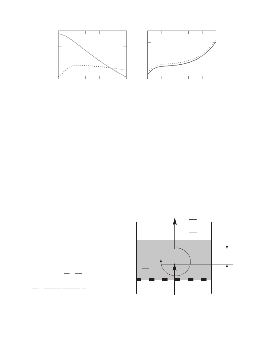
and
. Sa mple sim ula-
tion results for this case are plott ed in Figure 3.18.
Note that at the end of drying, the tempe ratur e in the
dryer increa ses excess ivel y due to con stant power
being sup plied to the internal he ater. The mod el
may serve as a tool to con trol the process , e.g., in-
crease the ventilat ion rate W
B
when drying beco mes
too slow or reduce the heater power when tempe ra-
ture be comes too high as in this case.
3.8.2 B
ATCH
F
LUID
B
ED
D
RYING
In this case the soli d pha se may be consider ed as
perfec tly mixe d, so it wi ll be described by an inp ut–
output mod el wi th accumul ation term. On the oth er
hand, the gas phase changes its parame ters progres -
sively as it trave ls through the bed. This situ ation is
shown in Figure 3.19.
Ther efore, gas phase will be de scribed by a DPM
with no accu mulation and the solid pha se will be
describ ed by an LPM with an accu mulation term .
The resul ting equ ations are:
dX
dt
¼
a
V
(1
«) r
S
1
H
Z
H
0
w
D
dh (3 : 121)
dY
dh
¼
S
W
B
w
D
a
V
(3 : 122)
d t
m
dt
¼
a
V
(1
«) r
S
1
c
S
þ c
Al
X
1
H
Z
H
0
[ q
(( c
A
c
Al
)t
m
þ Dh
v0
)w
D
]d h
(3 : 123)
dt
g
dh
¼
S
W
B
a
V
1
c
B
þ c
A
Y
[ q
þ c
A
( t
g
t
m
) w
D
] (3: 124)
Equation 3.122 and Equation 3.124 for the gas pha se
serve only to compute distribut ions of Y an d t
g
along
bed height , which is necessa ry to calcul ate q an d w
D
.
They can easil y be integ rated num erically, e.g., by the
Euler method , at each time step. The integrals in
Equation 3.121 and Equat ion 3.123 can be numeri c-
ally calculated, e.g., by the trapezoidal rule. This
allows Equation 3.121 and Equation 3.123 to be
solved by any ODE solver. The model has been
solved for a sample case and the results are shown
in
.
0
0.2
0.4
0.6
0.8
1
0
0.1
0.2
0.3
Time, h
X
, Y
, kg/kg
0
0.2
0.4
0.6
0.8
1
0
50
100
150
200
Time, h
t
m
, t
g
, ⬚
C
(a)
(b)
FIGURE 3.18 Solution of a batch oven dryer model—solid dry mass is 90 kg, internal heater power is 20 kW and air
ventilation rate is 0.1 kg/s (dry basis); external air humidity is 2 g/kg and temperature 208C: (a) moisture content X (solid line)
and air humidity Y (broken line); (b) material temperature t
m
(solid line) and air temperature t
g
(broken line).
d
h
d
X
d
t
d
t
m
d
t
W
B
W
B
Y
t
g
Y +
d
h
t
g
+
d
h
d
Y
d
h
d
t
g
d
h
m
S
FIGURE 3.19 Schematic of a batch fluid bed dryer.
ß
2006 by Taylor & Francis Group, LLC.
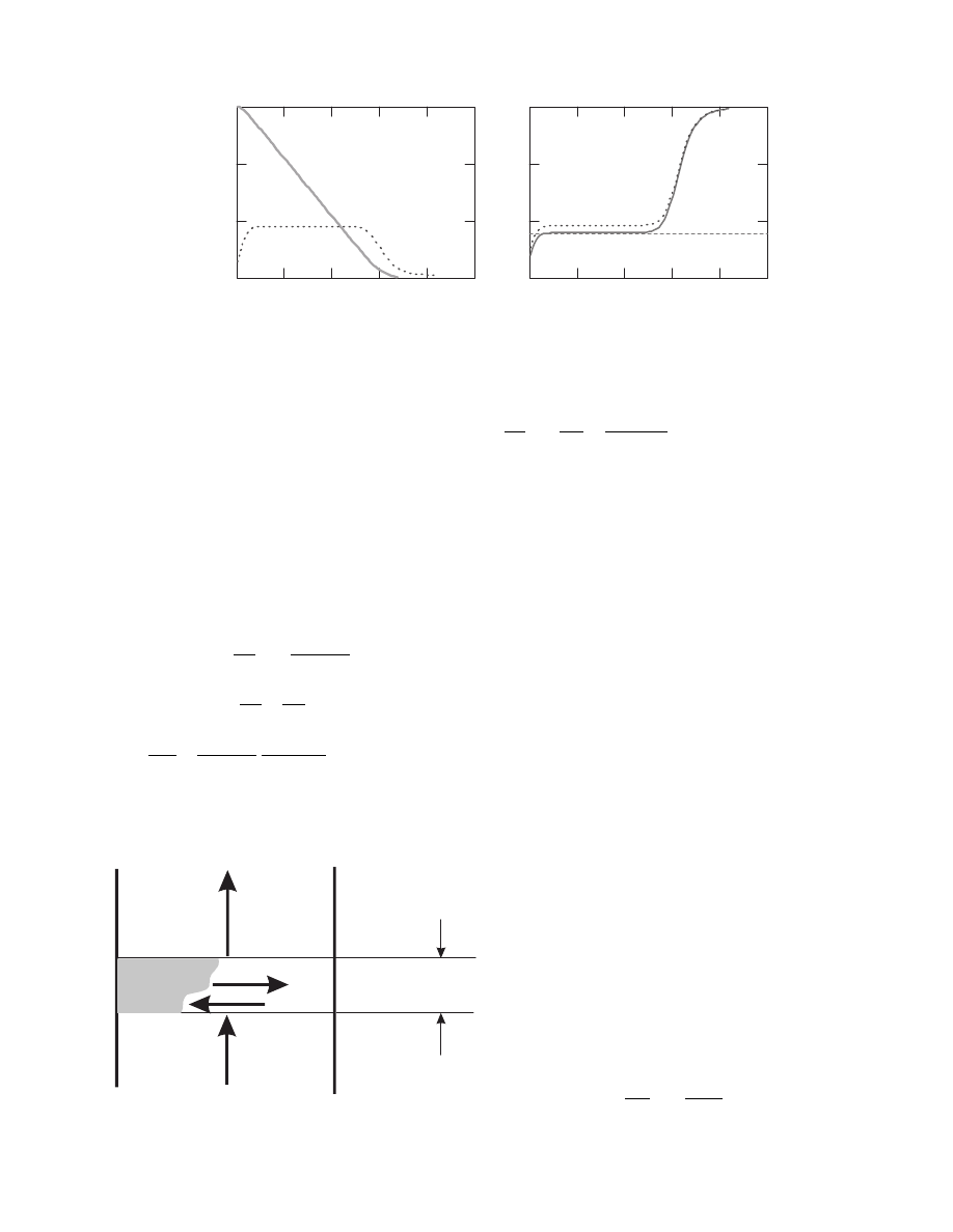
3.8.3 D
EEP
B
ED
D
RYING
In de ep be d drying solid pha se is stationar y and re-
mains in the dryer for a certain tim e whi le gas pha se
flows through it continuou sly (case 2a of
) .
Drying begins at the inlet end of gas and progres ses
through the entire bed . A typical desorpt ion wave
travels through the bed. The situatio n is sh own sche-
matical ly in Figure 3.21.
The above situatio n is described by the foll owing
set of equati ons:
dX
d t
¼
w
D
a
V
(1
«) r
S
(3 : 125)
dY
dh
¼
S
W
B
w
D
a
V
(3 : 126)
d t
m
dt
¼
a
V
(1
«) r
S
1
c
S
þ c
Al
X
¼ [ q ((c
A
c
Al
) t
m
þ D h
v0
) w
D
]
(3: 127)
dt
g
dh
¼
S
W
B
a
V
1
c
B
þ c
A
Y
[ q
þ c
A
( t
g
t
m
) w
D
] (3: 128)
The equatio ns can be solved by finite diff erence dis-
cretizat ion and a su itable numerica l techni que.
presents the resul ts of a sim ulation of drying
cereal grains in a thick bed using Ma thcad. Note
how a de sorption wave is formed , and also that the
solid in deeper regions of the be d init ially takes up
moisture from the air humidi fied during its pa ssage
through the entry region.
Give n a model togeth er with its method of solu-
tion it is relative ly easy to vary BCs, e.g., chan ge air
tempe rature in tim e or switch the gas flow from top to
bottom intermittent ly, a nd observe the beh avior of
the syst em.
3.9 MODELS FOR SEMICONTINUOUS
DRYERS
In some cases the dryers are operate d in such a way that
a batch of soli ds is loaded into the dryer and it progres -
sively mo ves through the dryer. New batches are
loaded a t specified time intervals and at the same mo-
ment dry batches are remove d at the other en d. Ther e-
fore, the mate rial is not mov ing continuous ly but by
step increm ents. This is a typic al situatio n in a tun-
nel dryer where trucks are loaded at one end of a tun nel
and unloaded at the other, as shown in
.
To simplify the case one can take an LPM for
each truck and a DPM for circulating air. As before,
we will neglect accumulation in the gas phase but of
course consider it in the solid phase. The resulting set
of equations is
dX
i
dt
¼
w
Di
A
i
m
Si
(3:129)
0
0
0.5
1
1.5
Drying time, h
X
, kg/kg
Y
2
*10, kg/kg
0
0
50
100
150
Drying time, h
t
m
, t
g
⬚
C
t
WB
1
2
3
4
5
1
2
3
4
5
FIGURE 3.20 Temporal changes of solid moisture content and temperature and exit air humidity and temperature in a
sample batch fluid bed dryer. Bed diameter 0.6 m, bed height 1.2 m, particle diameter 3 mm, particle density 1200 kg/m
3
, air
temperature 1508C, and humidity 1 g/kg.
d
h
W
B
Y+ dh
t
g
+ d
h
Y
W
B
d
Y
d
h
d
t
g
d
h
__
__
w
D
t
g
q
X
t
m
FIGURE 3.21 Schematic of batch drying in a deep layer.
ß
2006 by Taylor & Francis Group, LLC.
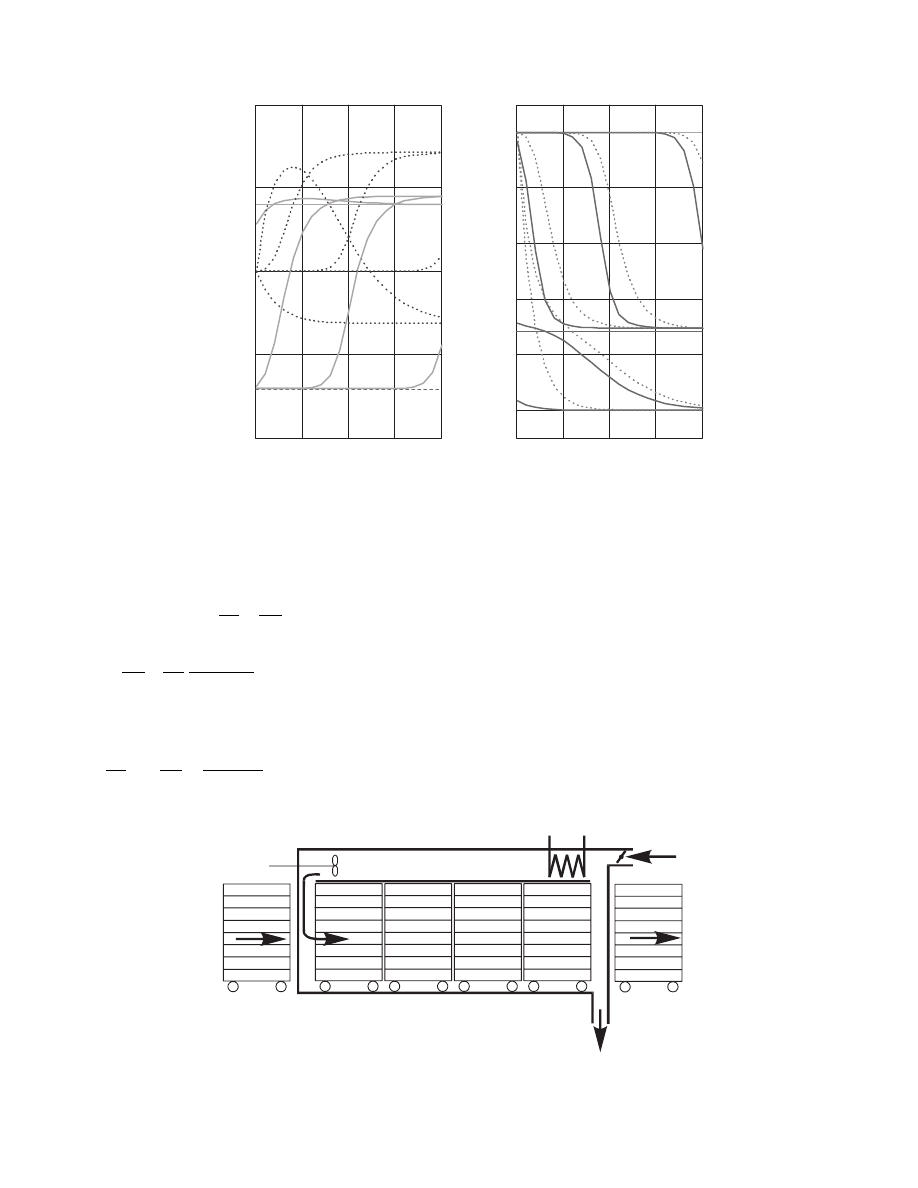
dY
dl
¼
S
W
B
w
D
a
V
(3:130)
dt
i
m
dt
¼
A
i
m
Si
1
c
S
þ c
Al
X
i
[q
i
((c
A
c
Al
)t
i
m
þ Dh
v0
)w
Di
]
(3:131)
dt
g
dl
¼
S
W
B
a
V
1
c
B
þ c
A
Y
[q
þ c
A
(t
g
t
m
)w
D
] (3:132)
where i is the number of a current truck. Additionally,
a balance equation for mixing of airstreams at fresh
air entry point is required. The semi-steady-state
solution is when a new cycle of temporal change of
X
i
and t
m
i
will be identical to the old cycle. In order to
converge to a semi–steady state the initial profiles of
X
i
and t
m
i
must be assumed. Usually a linear distribu-
tion between the initial and the final values is enough.
The profiles are adjusted with each iteration until a
cyclic solution is found.
0
0.05
0.1
0.15
0.2
0
0.1
0.2
0.3
0.4
(a)
(b)
Bed height, m
X
, kg/kg
Y
*10, kg/kg
X
e
0
0.05
0.1
0.15
0.2
20
30
40
50
60
70
Bed height, m
t
m
, t
g
, ⬚
C
t
WB
FIGURE 3.22 Simulation of deep bed drying of cereal grains: (a) moisture content profiles (solid lines) and gas humidity
profiles (broken lines); (b) material temperature (solid lines) and air temperature (broken lines). Initial solid temperature
208C and gas inlet temperature 708C. Profiles are calculated at 0.33, 1.67, 3.33, 6.67, and 11.67 min of elapsed time. X
e
is
equilibrium moisture content and t
WB
is wet-bulb temperature.
i
q
h
W
B
FIGURE 3.23 Schematic of a semicontinuous tunnel dryer.
ß
2006 by Taylor & Francis Group, LLC.
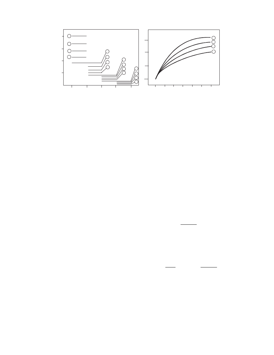
The so lution of this system of equa tions is sche-
matical ly shown in Figure 3.24 for semi -steady-s tate
operati on and four trucks in the dryer. In eac h truck
moisture content dro ps in time until the load–unl oad
time inter val. Then the truck is moved one position
forward so the last mo isture co ntent for this truck at
former pos ition becomes its init ial mois ture co ntent
at the ne w position. A practical a pplication of this
model for drying of grapes is present ed by Cace res-
Huambo and Men egalli (2002) .
3.10 SHORTCUT METHODS FOR DRYER
CALCULATION
When no data on sorpti onal propert ies, water diff u-
sivity, shrinka g e, etc. , are avail able, dryer design can
only be approxim ate, ne vertheless useful, as a first
approach . We will identi fy here two such situ ations.
3.10.1 D
RYING
R
ATE FROM
P
REDICTED
K
INETICS
3.10.1.1 Free Moisture
This case exists when dr ying of the prod uct entir ely
takes place in the constant drying rate period. It is
almost always possibl e when the soli d contain s un-
bound moisture. Tex tiles, miner als, and inorgani c
chemi cals are example s of such solids.
Let us investiga te a co ntinuous dryer calcul ation.
In this case soli d tempe ratur e will reach, dep ending on
a number of trans fer units in the dryer, a value between
AST and WBT, which can easily be calcul ated from
. Now mass and en-
ergy ba lances can be closed over the whol e dryer and
exit parame ters of air and mate rial obtaine d. Having
these, the average d solid an d gas temperatur es and
moisture content s in the dryer can be calculated. Fi-
nally the drying rate can be calcul ated from
, whi ch in turn allows one to calcul ate solid area in
the dr yer. Various aspect ratios of the dryer chambe r
can be designe d; one shou ld use judgme nt to calcul ate
dryer cross- section in such a way that air veloci ty will
not cause soli d entrai nment, etc.
3.10.1.2 Bound Moisture
In this case we can predict drying rate by assuming
that it is linea r, and at X
¼ X * drying rate is zero,
whereas at X
¼ X
cr
dry ing rate is w
DI
. The equ ation
of drying rate then be comes
w
D
¼ w
DI
X
X *
X
c
X *
¼ w
DI
F
(3 : 133)
This equati on can be used for calcul ation of drying
time in ba tch drying. Substi tuting this equ ation into
and integrati on from the initial X
0
to
final moisture content X
f
, the drying time is obtaine d
t
¼
m
S
Aw
DI
(X
c
X *) ln
X
0
X *
X
f
X *
(3 : 134)
Similarly , Equation 3.133 can be used in a mo del of a
continuous dryer.
3.10.2 D
RYING
R
ATE FROM
E
XPERIMENTAL
K
INETICS
Another simple case is when the drying curve has
been obtained experimentally. We will discuss both
batch and continuous drying.
L
X
L
Y
Truck 1
Truck 2
Truck 3
Truck 4
0
0
1
1
1
1
1
2
2
2
2
2
3
3
3
3
3
4
4
4
4
4
(a)
(b)
FIGURE 3.24 Schematic of the model solution for semicontinuous tunnel dryer for cocurrent flow of air vs. truck
direction—mass transfer only: (a) moisture content in trucks at specified equal time intervals; (b) humidity profiles at
specified time intervals. 1, 2, 3, 4—elapsed times.
ß
2006 by Taylor & Francis Group, LLC.
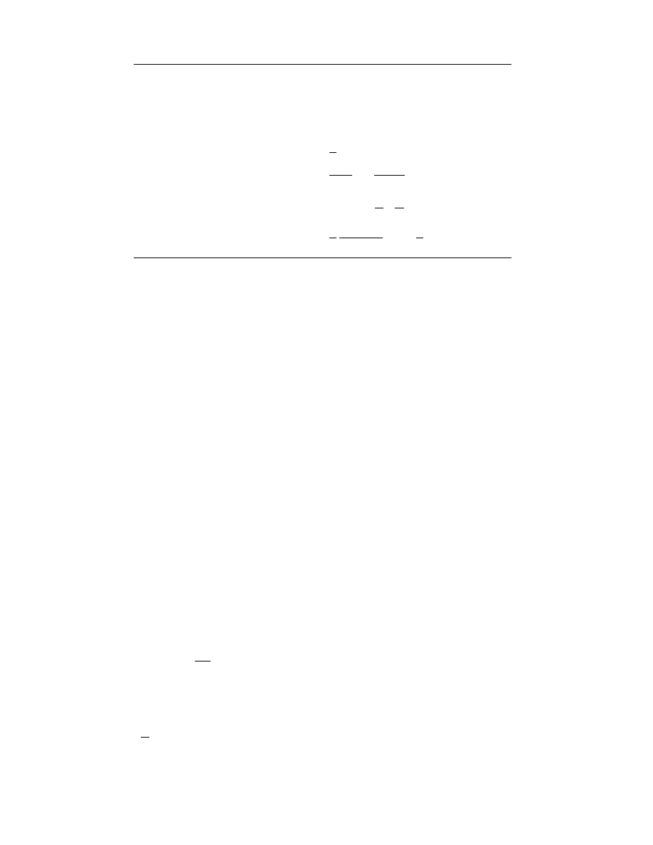
3.10.2.1 Batch Drying
We may assum e that if the solid size and drying
conditi ons in the indu strial dryer a re the same, the
drying time will also be the same as obtaine d experi -
menta lly. Other sim ple scali ng rules ap ply, e.g. , if a
batch fluid bed thickn ess is double of the experi men-
tal one, the dry ing time will a lso double .
3.10.2.2 Continuous Drying
Here the exp erimental drying kinetics can only be
used if mate rial flow in the dryer is of plug type. In
other words , it is as if the dryer served as a trans -
porter of a batch co ntainer wher e drying is identi cal
to that in the expe riment. How ever, when a certa in
degree of mixi ng of the solid pha se occu rs, parti cles of
the solid pha se exiting the dryer will have v arious
residen ce times and will theref ore differ in mois ture
content . In this case we c an only talk of average fina l
moisture con tent. To ca lculate this value we will use
methods of resi dence tim e distribut ion (RTD ) analy-
sis. If the emp irical drying kinetic s curve can be repre-
sented by the follo wing relationshi p:
X
¼ f (X
0
, t )
(3: 135)
and mean reside nce time by
t
r
¼
m
S
W
S
(3 : 136)
the average exit soli d mois ture con tent can be calcu-
lated using the external RTD function E as
X
¼
Z
1
0
E ( t )X ( X
0
,t ) dt (3 : 137)
Formula s for E functi on are present ed in Tabl e 3.3
for the most common flow models .
is an exempl ary compari son of a batch
and real drying c urves. As can be seen, dr ying tim e in
real flow co nditions is approxim ately 50% longer
here.
3.11 SOFTWARE TOOLS FOR DRYER
CALCULATIONS
Menshu tina and Kudra (2001) present 17 commer cial
and semicomm ercia l program s for drying calcul ations
that they were able to identi fy on the market . Only a
few of them perfor m process calculati ons of dryers
includin g dryer dimens ioning, usually for fluid bed
dryers . Typical ly a program for dryer calcul ations
perfor ms ba lancin g of heat and mass and, if dimen-
sionin g is possibl e, the pr ogram requires empir ical
coeffici ents, whic h the us er ha s to supp ly. Similarl y,
the dr ying pro cess is de signed in commer cial pro cess
simulat ors used in ch emical and process engineer ing.
A program that does all calcul ations presented in this
chapter does not exist. How ever, wi th presen t-day
computer technol ogy, co nstruction of su ch so ftware
is possibl e; dryPAK (Silva and Correa, 199 8;
Pakowski , 1 999) is a program that evolves in this
direction. The main concept in dr yPAK is that all
models share the same da tabase of hum id ga s, mois t
material prop erties, methods for calcul ation of dry ing
rate, etc. The resul ts are also visual ized in the same
way.
,
, an d
wer e in fact prod uced with dryPAK .
General-purpose mathematical software can greatly
simplify solvin g new models of not-too-com plex
structure. Calculat ions shown in
,
produced with Mathcad. Mathcad or MATLAB can
TABLE 3.3
External RTD Function for Selected Models of Flow
Model of Flow
E Function
Plug flow
E(t)
¼ d(t t
r
)
(3.138)
Perfectly mixed flow
E(t)
¼
1
t
r
e
t=t
r
(3.139)
Plug flow with axial dispersion
E(t)
¼
1
s
ffiffiffiffiffiffi
2p
p
exp
(t
t
r
)
2
2s
2
!
(3.140)
where for Pe $ 10,
s
2
t
2
r
¼
2
Pe
n-Perfectly mixed uniform beds
E(t)
¼
n
t
r
(n(t=t
r
) )
n
1
(n
1)!
exp
n
t
t
r
(3.141)
ß
2006 by Taylor & Francis Group, LLC.
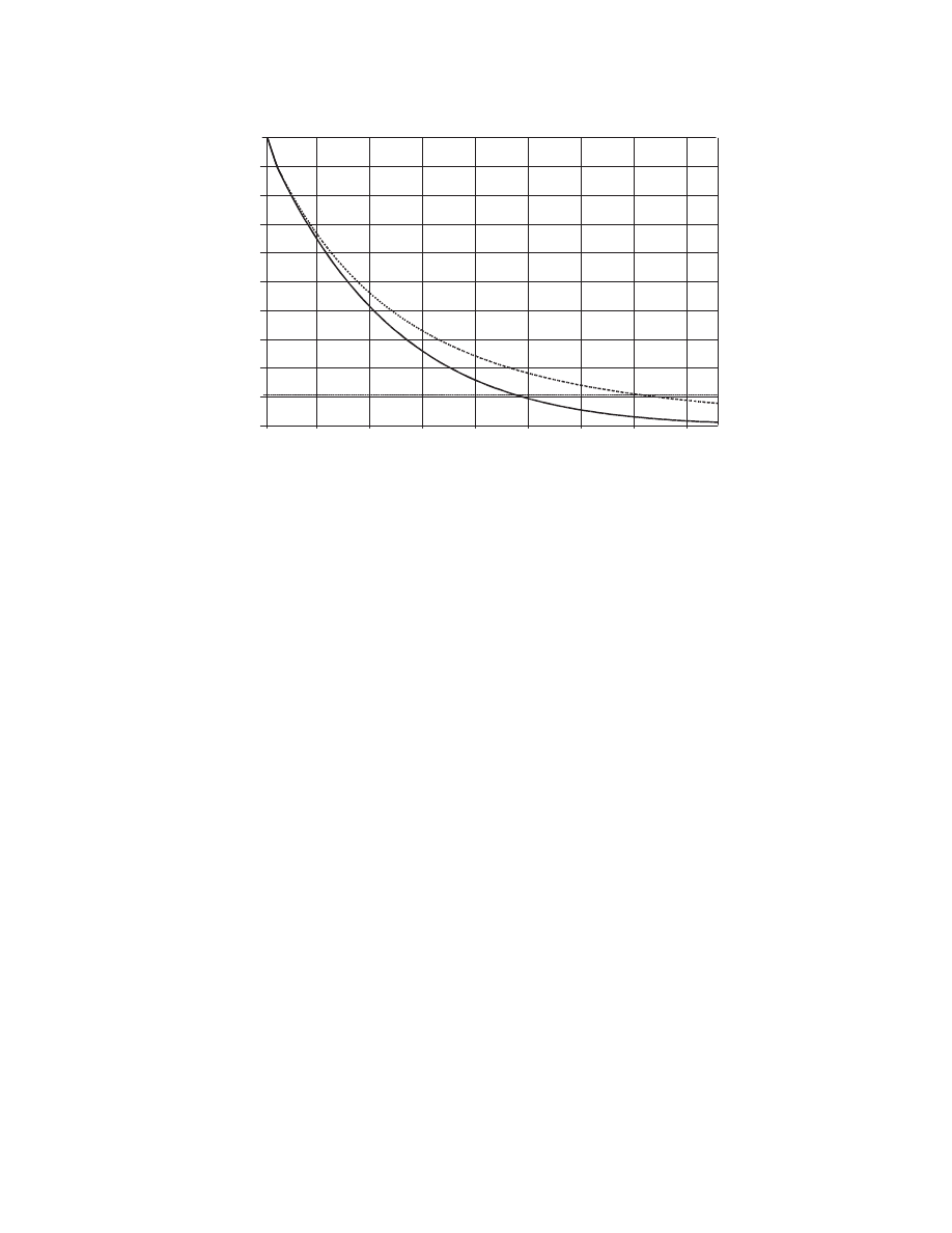
signific antly reduce the effort involv ed with numeri cal
solution s of equatio n syst ems as they co ntain a multi-
tude of solver s for both algebr aic and different ial eq ua-
tions. Prob lems that woul d requir e severa l da ys of
work can now be solved within hours. To let the read er
get acqu ainted with this tool severa l Mathcad files
contai ning selec ted solut ions of problem s presen ted
in this sectio n wi ll be made available at
. Both MATLAB a nd Mathcad
offer associated tools for visual modeli ng of dy namic
systems (Sim ulink and VisiSi m, respect ivel y) that
make simulat ion of batch system even easie r.
3.12 CONCLUSION
In this chapter we have illustrated how dry er calcul a-
tions can be made by con structing a mo del of a dr yer
and solvin g it using appropri ate num erical methods .
Using general-pu rpose mathe matical softwar e solving
models is a task that can be handled by any engineer .
The resul ts can be obtaine d in a short time and pr o-
vide a so und ba sis for mo re detailed dryer calcul a-
tions. For more advan ced an d spec ialized drye r
design de dicated softwar e shou ld be sought. How -
ever, the que stion of how to obt ain the ne cessary
propert y data of dried mate rials remai ns. Thi s que s-
tion is as important now as it was before since ve ry
little ha s been done in the area of mate rials databas es.
The data are spread over the literatu re and, in the
case of unsuccess ful search, an exp erimental deter-
mination of the mis sing da ta is nec essary.
NOMENCLATURE
A
interfacial area of phase contact, m
2
a,b,c
constants of GAB equation
a
V
characteristic interfacial area per unit volume
of dryer, 1/m
c
specific heat, kJ/(kg K)
D
diffusivity, m
2
/s
E
axial dispersion coefficient, m
2
/s
E
external RTD function
f
ratio of drying rates in CDC equation
G
shear modulus, Pa
h
specific enthalpy per unit mass of species,
kJ/kg
Dh
s
latent heat of sorption, kJ/kg
Dh
v
latent heat of vaporization, kJ/kg
i
specific enthalpy per dry basis, kJ/kg
k
permeability, m
2
k
Y
mass transfer coefficient, kg/(m
2
s)
L
total length, m
l
running length, m
M
molar mass, kg/kmol
m
mass holdup, kg
p
vapor pressure, Pa
P
0
total pressure, Pa
q
heat flux, kW/m
2
R
maximum radius, m
R
universal gas constant, kJ/(kmol K)
r
actual radius, m
S
cross-sectional area normal to flow direction,
m
2
0.0
0.0
0.1
0.2
0.3
0.4
0.5
0.6
0.7
0.8
0.9
1.0
0.5
1.0
1.5
2.0
2.5
3.0
3.5
4.0
Drying curve influenced by RTD
calculated by CDC for sand
Drying time ca. 8.48 min
dryPAK v.3.6
Φ final
Φ, −
q
, −
FIGURE 3.25 Experimental (solid line) and actual (broken line) drying kinetic curves for three tanks in series model of flow.
u
is the ratio of the actual to mean residence times, F is dimensionless moisture content.
ß
2006 by Taylor & Francis Group, LLC.

s shrinka ge coeffici ent
t tempe ratur e, 8 C
T absolut e temperatur e, K
W mass flowra te, kg /s
w
D
drying rate, kg/(m
2
s)
X mois ture con tent per dry basis, kg/kg
x coord inate in Car tesian syst em, m
Y absolut e humidi ty per dry basis, kg/kg
V total volume , m
3
a
heat transfer coeffici ent, kW/(m
2
K)
d
Dirac delta function
«
voidage
F
dimens ionles s mois ture content
¼ (X – X*)/
( X
c
– X*)
f
w
relative humidi ty
l
therm al con ductivity , kW /(m K)
m
viscos ity, Pa s
n
Poisson’ s ratio
r
densit y, kg/m
3
t
time, s
S
UBSCRIPTS AND
S
UPERSCRIPTS
A mois ture
AS adiabat ic satur ation
B dry gas
c critical (for moisture content )
g humid gas
i at inter face
m wet solid
m mean value
s at satur ation
S dry solid
WB wet bulb
v vapor pha se
* in equilibrium
– space average d
REFERENCES
Berg C.G., Kemp I.C., Stenstro¨ m S., Wimmerstedt R.,
2002, Transport equations for moist air at elevated
wet bulb temperatures, in The 13th International
Drying Symposium , Beijing, China, Conference Pro-
ceedings, pp. 135–144.
Caceres-Huambo B.N., Menegalli F.C., 2002, Simulation
and optimization of semi-continuous tray tunnel
dryers for grapes, in Drying’2002 , Beijing, A 471–480.
Crank J., 1975, The Mathematics of Diffusion , Clarendon
Press, Oxford.
Ginzburg A.S., Savina I.M., 1982, Mass transfer character-
istics of food products, Handbook, (in Russian),
LiPP, Moscow.
Grosvenor W.M., 1907, Calculations for dryer design,
Trans. A.I.Ch.E ., 1, 184–202.
Hallstro¨ m A., Wimmerstedt R., 1983, Drying of porous
granular materials, Chem. Eng. Sci ., 38, 1507–
1516.
Hasatani M., Itaya Y., 1996, Drying-induced strain and
stress: a review, Drying Technol., 14(5), 1011–1040.
Iglesias H.A., Chirife J., 1984, Handbook of Food Isotherms,
Academic Press, New York.
Jayas D.S., Cenkowski S., Pabis S., Muir W.E., 1991, Re-
view of thin-layer drying and wetting equations,
Drying Technol., 9(3), 551–588.
Kechaou N., Roques M., 1990, A model for convective
drying of nonporous shrinking spheres, IDS90, vol
1, p. 369–373.
Keey, R.B., 1978, Introduction to Industrial Drying Oper-
ations, Pergamon Press, Oxford.
Langrish T., Bahu R., Reay D., 1991, Drying kinetics of
particles from thin layer drying experiments, Trans.
IChemE, 69A(1–8), 417–424.
Lewis W.K., 1921, The rate of drying of solid materials,
J. Ind. Eng. Chem., 13, 427–433.
Lima A.G.B., Nebra S.A., Queiroz M.R., 2001, Theoretical
analysis of the diffusion process inside prolate
spheroidal solids, Drying Technol., 18(1–2), 21–48.
Luikov A.V., 1966, Heat and Mass Transfer in Capillary-
Porous Bodies, Pergamon Press, Oxford.
Marinos-Kouris D., Maroulis Z.B., 1995, Transport prop-
erties in the drying of solids, in Handbook of Indus-
trial Drying, A.S. Mujumdar (Ed.), 2nd ed., Vol. 2,
Marcel Dekker, New York, pp. 113–159.
Menshutina N.V., Kudra T., 2001, Computer aided
drying technologies, Drying Technol., 19(8), 1825–
1849.
Mollier R., 1923, Ein neues Diagram fuer Dampfluftge-
mische, Zeits. VDI, 67, 869–872.
Nijdam J., Keey R.B., 2000, Impact of variations in wood
density on kiln drying softwood boards, Bull. Pol.
Acad. Sci. (Techn. Sci.), 48(3), 301–313.
Nikitina L.M., 1968, Thermodynamic parameters and co-
efficients of mass transfer in wet solids (in Russian),
Energia, Moscow.
Page C., 1949, Factors Influencing the Maximum Rates of
Drying Shelled Corn in Layer, M.Sc. thesis, Depart-
ment of Agricultural Engineering, Purdue Univer-
sity, West Lafayette.
Pakowski Z., 1986, Computer drawing of enthalpy-humid-
ity charts, Hung. J. Ind. Chem., 14, 225.
Pakowski Z., 1999, Simulation of the process of convective
drying: identification of generic computation rou-
tines and their implementation in computer code
dryPAK, Comput. Chemical Eng., 23(1), S719–S722.
Pakowski Z., Mujumdar A.S., 1987 (I ed.), 1995 (II ed.)
Basic process calculations in drying, in Handbook of
Industrial Drying, A.S. Mujumdar (Ed.), Marcel
Dekker, New York.
Perre P., Turner I., 1999, A 3D version of TransPore: a
comprehensive heat and mass transfer computa-
ß
2006 by Taylor & Francis Group, LLC.

tional model for simulation the drying of porous
media, Int. J. Heat Mass Transfer, 42(24), 4501–
4521.
Perre P., Turner I. (Eds.), 2000, Mathematical Modeling and
Numerical Techniques in Drying Technology, Marcel
Dekker, New York.
Reid R.C., Prausnitz J.M., Polling B.E., 1987, The Prop-
erties of Gases and Liquids, McGraw-Hill, New
York.
Shallcross D.C, 1994, Construction of psychometric charts
for systems other than water vapour in air, Trans.
IChemE, 72, A, 763–776.
Silva M.A., Correa J.L.G., 1998, Using dryPAK to simulate
drying processes, IDS98, A, 303–310.
Soininen M., 1986, A perspectively transformed psychro-
metric chart and its applications to drying calcula-
tions, Drying Technol., 4(2), 295–305.
Strumillo C., Pakowski Z., Zylla R., 1986, Design of FB
and VFB dryers by computer methods (in Russian),
Zhurn. Prikl. Khim., 9, 2108.
Treybal R.E., 1980, Mass-Transfer Operations, 3rd ed.,
McGraw-Hill, New York.
Yaws C.L., 1999, Chemical Properties Handbook, McGraw-
Hill, New York.
ß
2006 by Taylor & Francis Group, LLC.
Document Outline
- Table of Contents
- Chapter 003: Basic Process Calculations and Simulations in Drying
- 3.1 Introduction
- 3.2 Objectives
- 3.3 Basic Classes of Models and Generic Dryer Types
- 3.4 General Rules for a Dryer Model Formulation
- 3.4.1 Mass and Energy Balances
- 3.4.2 Constitutive Equations
- 3.4.3 Auxiliary Relationships
- 3.4.3.1 Humid Gas Properties and Psychrometric Calculations
- 3.4.3.2 Relations between Absolute Humidity, Relative Humidity, Temperature, and Enthalpy of Humid Gas
- 3.4.3.3 Calculations Involving Dew-Point Temperature, Adiabatic-Saturation Temperature, and Wet-Bulb Temperature
- 3.4.3.4 Construction of Psychrometric Charts
- 3.4.3.5 Wet Solid Properties
- 3.4.4 Property Databases
- 3.5 General Remarks on Solving Models
- 3.6 Basic Models of Dryers in Steady State
- 3.7 Distributed Parameter Models for the Solid
- 3.8 Models for Batch Dryers
- 3.9 Models for Semicontinuous Dryers
- 3.10 Shortcut Methods for Dryer Calculation
- 3.11 Software Tools for Dryer Calculations
- 3.12 Conclusion
- Nomenclature
- References
Wyszukiwarka
Podobne podstrony:
Chemotherapy Dose Calculation and Administration in Exotic Animal Species
Ionic liquids as solvents for polymerization processes Progress and challenges Progress in Polymer
Combined Radiant and Conductive Vacuum Drying in a Vibrated Bed (Shek Atiqure Rahman, Arun Mujumdar)
Influence of different microwave seed roasting processes on the changes in quality and fatty acid co
Use of exponential, Page’s and diffusional models to simulate the drying kinetics of kiwi fruit
BASIC MALTESE GRAMMAR AND DIC (G Falzon)
Degradable Polymers and Plastics in Landfill Sites
Estimation of Dietary Pb and Cd Intake from Pb and Cd in blood and urine
Aftershock Protect Yourself and Profit in the Next Global Financial Meltdown
General Government Expenditure and Revenue in 2005 tcm90 41888
Basic AC Generators and Motors
Basic setting for caustics effect in C4D
A Guide to the Law and Courts in the Empire
D Stuart Ritual and History in the Stucco Inscription from Temple XIX at Palenque
Exile and Pain In Three Elegiac Poems
A picnic table is a project you?n buy all the material for and build in a?y
Economic and Political?velopment in Zimbabwe
więcej podobnych podstron