
Algorithm Collections for Digital Signal Processing
Applications Using Matlab

Algorithm Collections
for Digital Signal Processing
Applications Using Matlab
E.S. Gopi
National Institute of Technology, Tiruchi, India

A C.I.P. Catalogue record for this book is available from the Library of Congress.
ISBN 978-1-4020-6409-8 (HB)
ISBN 978-1-4020-6410-4 (e-book)
Published by Springer,
P.O. Box 17, 3300 AA Dordrecht, The Netherlands.
www.springer.com
Printed on acid-free paper
All Rights Reserved
© 2007 Springer
No part of this work may be reproduced, stored in a retrieval system, or transmitted in
any form or by any means, electronic, mechanical, photocopying, microfilming, recording
or otherwise, without written permission from the Publisher, with the exception
of any material supplied specifically for the purpose of being entered
and executed on a computer system, for exclusive use by the purchaser of the work.

This book is dedicated to
my Wife G.Viji
and my Son V.G.Vasig

Contents
Preface xiii
Acknowledgments x
Chapter 1 ARTIFICIAL INTELLIGENCE
1 Particle Swarm Algorithm
1
1-1 How are the Values of ‘x’ and ‘y’ are Updated
in Every Iteration?
2
1-2 PSO Algorithm to Maximize the Function F(X, Y, Z)
4
1-3 M-program for PSO Algorithm
6
1-4 Program Illustration
8
2 Genetic Algorithm
9
2-1 Roulette Wheel Selection Rule
10
2-2 Example
11
2-2-1 M-program for genetic algorithm
11
2-2-2 Program illustration
13
2-3 Classification of Genetic Operators
15
2-3-1 Simple crossover
16
2-3-2 Heuristic crossover
16
2-3-3 Arith crossover
17
3 Simulated Annealing
18
3-1 Simulated Annealing Algorithm
19
3-2 Example
19
3-3 M-program for Simulated Annealing
23
v
vii

4 Back Propagation Neural Network
24
4-1 Single Neuron Architecture
25
4-2 Algorithm
27
4-3 Example
29
4-4 M-program for Training the Artificial Neural Network
for the Problem Proposed in the Previous Section
31
5 Fuzzy Logic Systems
32
5-1 Union and Intersection of Two Fuzzy Sets
32
5-2 Fuzzy Logic Systems
33
5-2-1 Algorithm
35
5-3 Why Fuzzy Logic Systems?
38
5-4 Example
39
5-5 M-program for the Realization of Fuzzy Logic System
for the Specifications given in Section 5-4
41
6 Ant Colony Optimization
44
6-1 Algorithm
44
6-2 Example
48
6-3 M-program for Finding the Optimal Order using Ant Colony
Technique for the Specifications given in the Section 6-2
50
Chapter 2 PROBABILITY AND RANDOM PROCESS
1 Independent Component Analysis
53
1-1 ICA for Two Mixed Signals
53
1-1-1 ICA algorithm
62
1-2 M-file for Independent Component Analysis
65
2 Gaussian Mixture Model
68
2-1 Expectation-maximization Algorithm
70
2-1-1 Expectation stage
71
2-1-2 Maximization stage
71
2-2 Example
72
2-3 Matlab Program
73
2-4 Program Illustration
76
3 K-Means Algorithm for Pattern Recognition
77
3-1 K-means Algorithm
77
3-2 Example
77
3-3 Matlab Program for the K-means Algorithm Applied
for the Example given in Section 3-2
78
4 Fuzzy K-Means Algorithm for Pattern Recognition
79
4-1 Fuzzy K-means Algorithm
80
4-2 Example
81
4-3 Matlab Program for the Fuzzy k-means Algorithm Applied
for the Example given in Section 4-2
83
viii
Contents

5 Mean and Variance Normalization
84
5-1 Algorithm
84
5-2 Example 1
85
5-3 M-program for Mean and Variance Normalization
86
Chapter 3 NUMERICAL LINEAR ALGEBRA
87
1 Hotelling Transformation
87
1-1 Diagonalization of the Matrix ‘CM’
88
1-2 Example
88
1-3 Matlab Program
90
2 Eigen Basis
91
2-1 Example 1
91
3 Singular Value Decomposition (SVD)
93
3-1 Example
94
4 Projection Matrix
95
4-1 Projection of the Vector ‘a’ on the Vector ‘b’
95
4-2 Projection of the Vector on the Plane Described
by Two Columns Vectors of the Matrix ‘X’
96
4-2-1 Example
97
4-2-2 Example 2
98
5 Orthonormal Vectors
100
5-1 Gram-Schmidt Orthogonalization procedure
100
5-2 Example
101
5-3 Need for Orthonormal Basis
101
5-4 M-file for Gram-Schmidt Orthogonalization Procedure
103
6 Computation of the Powers of the Matrix ‘A’
103
7 Determination of K
th
Element in the Sequence
104
8 Computation of Exponential of the Matrix ‘A’
107
8.1 Example
107
9 Solving Differential Equation Using Eigen decomposition
108
10 Computation of Pseudo Inverse of the Matrix
109
11 Computation of Transformation Matrices
111
11-1 Computation of Transformation Matrix for the Fourier
Transformation
113
11-2 Basis Co-efficient transformation
115
11-3 Transformation Matrix for Obtaining Co-efficient
of Eigen Basis
117
11-4 Transformation Matrix for Obtaining Co-efficient
of Wavelet Basis
117
12 System Stability Test Using Eigen Values
118
13 Positive Definite Matrix test for Minimal Location
of the Function f (x1, x2, x3, x4…xn)
119
ix
Contents

x
14 Wavelet Transformation Using Matrix Method
119
14-1 Haar Transformation
120
14-1-1 Example
122
14-1-2 M-file for haar forward and inverse
transformation 125
14-2 Daubechies-4 Transformation
127
14-2-1 Example
128
14-2-2 M-file for daubechies 4 forward
and inverse transformation
131
Chapter 4 SELECTED APPLICATIONS
135
1 Ear Pattern Recognition Using Eigen Ear
135
1-1 Algorithm
135
1-2 M-program for Ear Pattern Recognition
138
2 Ear Image Data Compression using Eigen Basis
141
2-1 Approach
141
2-2 M-program for Ear Image Data Compression
143
3 Adaptive Noise Filtering using Back Propagation
Neural Network
145
3-1 Approach
146
3-2 M-file for Noise Filtering Using ANN
147
3-3 Program Illustration
149
4 Binary Image Rotation Using Transformation Matrix
150
4-1 Algorithm
151
4-2 M-program for Binary Image Rotation with 45 Degree
Anticlockwise Direction
152
5 Clustering Texture Images Using K-means Algorithm
152
5-1 Approach
153
5-2 M-program for Texture Images Clustering
155
6 Search Engine Using Interactive Genetic Algorithm
156
6-1 Procedure
156
6-2 Example
158
6-3 M-program for Interactive Genetic Algorithm
160
6-4 Program Illustration
165
7 Speech Signal Separation and Denoising Using Independent
Component Analysis
166
7-1 Experiment 1
166
7-2 Experiment 2
167
7-3 M-program for Denoising
169
Contents
1-3 Program
Illustration
140

xi
8 Detecting Photorealistic Images using ICA Basis
170
8-1 Approach
171
8-1-1 To classify the new image into one among the
photographic or photorealistic image
171
8-2 M-program for Detecting Photo Realistic Images
Using ICA basis
172
8-3 Program Illustration
174
9 Binary Image Watermarking Using Wavelet Domain
of the Audio Signal
9-1 Example
175
9-2 M-file for Binary Image Watermarking
in Wavelet Domain of the Audio Signal
176
9-3 Program Illustration
180
Appendix
183
Index 189
Contents
175

Preface
The Algorithms such as SVD, Eigen decomposition, Gaussian Mixture
Model, PSO, Ant Colony etc. are scattered in different fields. There is the
need to collect all such algorithms for quick reference. Also there is the need
to view such algorithms in application point of view. This Book attempts to
satisfy the above requirement. Also the algorithms are made clear using
MATLAB programs. This book will be useful for the Beginners Research
scholars and Students who are doing research work on practical applications
of Digital Signal Processing using MATLAB.
xiii

Acknowledgments
I am extremely happy to express my thanks to the Director
Dr M.Chidambaram, National Institute of Technology Trichy India for his
support. I would also like to thank Dr B.Venkatramani, Head of the
Electronics and Communication Engineering Department, National Institute
of Technology Trichy India and Dr K.M.M. Prabhu, Professor of the
Electrical Engineering Department, Indian Institute of Technology Madras
India for their valuable suggestions. Last but not least I would like to thank
those who directly or indirectly involved in bringing up this book
sucessfully. Special thanks to my family members father Mr E.Sankara
subbu, mother Mrs E.S.Meena, Sisters R.Priyaravi, M.Sathyamathi,
E.S.Abinaya and Brother E.S.Anukeerthi.
Thanks
E.S.Gopi
xv

Chapter 1
ARTIFICIAL INTELLIGENCE
Algorithm Collections
1.
PARTICLE SWARM ALGORITHM
Consider the two swarms flying in the sky, trying to reach the particular
destination. Swarms based on their individual experience choose the proper
path to reach the particular destination. Apart from their individual
decisions, decisions about the optimal path are taken based on their
neighbor’s decision and hence they are able to reach their destination faster.
The mathematical model for the above mentioned behavior of the swarm is
being used in the optimization technique as the Particle Swarm Optimization
Algorithm (PSO).
For example, let us consider the two variables ‘x’ and ‘y’ as the two
swarms. They are flying in the sky to reach the particular destination (i.e.)
they continuously change their values to minimize the function (x-10)
2
+(y-
5)
2
. Final value for ‘x’ and ‘y’ are 10.1165 and 5 respectively after 100
iterations.
The Figure 1-1 gives the closed look of how the values of x and y are
changing along with the function value to be minimized. The minimization
function value reached almost zero within 35 iterations. Figure 1-2 shows
the zoomed version to show how the position of x and y are varying until
they reach the steady state.
1
2 Chapter
1
Figure 1-1.
PSO Example zoomed version
Figure 1-2. PSO Example
1.1
How are the Values of ‘x and y’ are Updated
The vector representation for updating the values for x and y is given in
Figure 1-3. Let the position of the swarms be at ‘a’ and ‘b’ respectively as
shown in the figure. Both are trying to reach the position ‘e’. Let ‘a’ decides
to move towards ‘c’ and ‘b’ decides to move towards ‘d’.
The distance between the position ‘c’ and ‘e’ is greater than the distance
between ‘d’ and ‘e’. so based on the neighbor’s decision position ‘d’ is
treated as the common position decided by both ‘a’ and ‘b’. (ie) the position
‘c’ is the individual decision taken by ‘a’, position ‘d’ is the individual
decision taken by ‘b’ and the position ‘d’ is the common position decided by
both ‘a’ and ‘b’.
in Every Iteration?

1. Artificial Intelligence
3
‘a’ based on the above knowledge, finally decides to move towards the
position ‘g’ as the linear combination of ‘oa’ , ‘ac’ and ‘ad’ . [As ‘d’ is the
common position decided].The linear combination of ‘oa’ and scaled ‘ac’
(ie) ‘af’ is the vector ‘of’. The vector ‘of’ combined with vector ‘fg’ (ie)
scaled version of ‘ad’ to get ‘og’ and hence final position decided by ‘a’ is
‘g’.
Similarly, ‘b’ decides the position ‘h’ as the final position. It is the linear
combination of ‘ob’ and ‘bh’(ie) scaled version of ‘bd’. Note as ‘d’ is the
common position decided by ‘a’ and ‘b’, the final position is decided by
linear combinations of two vectors alone.
Thus finally the swarms ‘a’ and ‘b’ moves towards the position ‘g’ and
‘h’ respectively for reaching the final destination position ‘e’. The swarm ‘a’
and ‘b’ randomly select scaling value for linear combination. Note that ‘oa’
and ‘ob’ are scaled with 1 (ie) actual values are used without scaling. Thus
the decision of the swarm ‘a’ to reach ‘e’ is decided by its own intuition
along with its neighbor’s intuition.
Now let us consider three swarms (A,B,C) are trying to reach the
particular destination point ‘D’. A decides A’, B decides B’ and C decides
C’ as the next position. Let the distance between the B’ and D is less
compared with A’D and C’ and hence, B’ is treated as the global decision
point to reach the destination faster.
Thus the final decision taken by A is to move to the point, which is the
linear combination of OA, AA’ and AB’. Similarly the final decision taken
Figure 1-3. Vector Representation of PSO Algorithm

4 Chapter
1
by B is to move the point which is the linear combination of OB, BB’. The
final decision taken by C is to move the point which is the linear
combination of OC, CC’ and CB’.
1.2
PSO Algorithm to Maximize the Function F (X, Y, Z)
1. Initialize the values for initial position a, b, c, d, e
2. Initialize the next positions decided by the individual swarms as a’, b’, c’
d’ and e’
3. Global decision regarding the next position is computed as follows.
Compute f (a’, b, c, d, e), f (a, b’, c, d, e), f (a, b, c’, d, e), f (a, b, c, d’, e)
and f (a, b, c, d, e’). Find minimum among the computed values. If f (a’,
b, c, d, e) is minimum among all, the global position decided regarding
the next position is a’. Similarly If f (a, b’, c, d, e) is minimum among all,
b’ is decided as the global position regarding the next position to be
shifted and so on. Let the selected global position is represented ad
‘global’
4. Next value for a is computed as the linear combination of ‘a’ , (a’-a) and
(global-a) (ie)
• nexta = a+ C1 * RAND * (a’ –a) + C2 * RAND * (global –a )
• nextb = b+ C1 * RAND * (b’ –b) + C2 * RAND * (global –b)
• nextc = c+ C1 * RAND * (c’ –c) + C2 * RAND * (global –c )
• nextd = d+ C1 * RAND * (d’ –d) + C2 * RAND * (global –d )
• nexte = e+ C1 * RAND * (e’ –e) + C2 * RAND * (global –e )
5. Change the current value for a, b, c, d and e as nexta, nextb, nextc, nextd
and nexte
6. If f (nexta, b, c, d, e) is less than f (a’, b, c, d, e) then update the value for
a’ as nexta, otherwise a’ is not changed.
If f (a, nextb, c, d, e) is less than f (a, b’, c, d, e) then update the value for
b’ as nextb, otherwise b’ is not changed
If f (a, b, nextc, d, e) is less than f (a, b, c’, d, e) then update the value
for c’ as nextc, otherwise c’ is not changed

1. Artificial Intelligence
5
7. Repeat the steps 3 to 6 for much iteration to reach the final decision.
The values for ‘c1’,’c2’ are decided based on the weightage given to
individual decision and global decision respectively.
Let
Δa(t) is the change in the value for updating the value for ‘a’ in t
iteration, then nexta at (t+1)th iteration can be computed using the following
formula. This is considered as the velocity for updating the position of the
swarm in every iteration.
‘w ( t )’ is the weight at t
th
iteration. The value for ‘w’ is adjusted at every
iteration as given below, where ‘iter’ is total number of iteration used.
w(t+1)=w(t)-t*w(t)/(iter).
Decision taken in the previous iteration is also used for deciding the next
position to be shifted by the swarm. But as iteration increases, the
contribution of the previous decision is decreases and finally reaches zero in
the final iteration.
If f (a, b, c, nextd, e) is less than f (a, b, c, d’, e) then update the value
for d’ as nextd, otherwise d’ is not changed
If f (a, b, c, d, nexte) is less than f (a, b, c, d, e’) then update the value
for e’ as nexte, otherwise e’ is not changed
th
nexta (t+1) = (t) +
a(t+1) = c1 * rand * (a’ –a ) + c2 * rand * ( global –a ) +
w(t)*
Δa(t)
Δ
a(t+1)
Δ
where
a

6 Chapter
1
1.3
M – program for PSO Algorithm
psogv .m
function [value]=psogv(fun,range,ITER)
%psogv.m
%Particle swarm algorithm for maximizing the function fun with two variables x
%and y.
%Syntax
%[value]=psogv(fun,range,ITER)
%example
%fun='f1'
%create the function fun.m
%function [res]=fun(x,y)
%res=sin(x)+cos(x);
%range=[-pi pi;-pi pi];
%ITER is the total number of Iteration
error=[];
vel1=[];
vel2=[];
%Intialize the swarm position
swarm=[];
x(1)=rand*range(1,2)+range(1,1);
y(1)=rand*range(2,2)+range(2,1);
x(2)=rand*range(1,2)+range(1,1);
y(2)=rand*range(2,2)+range(2,1);
%Intialize weight
w=1;
c1=2;
c2=2;
%Initialize the velocity
v1=0;%velocity for x
v2=0;%velocity for y
for i=1:1:ITER
[p,q]=min([f1(fun,x(2),y(1)) f1(fun,x(1),y(2))]);
if (q==1)
capture=x(2);
else
capture=y(2);
end

1. Artificial Intelligence
7
Continued…
v1=w*v1+c1*rand*(x(2)-x(1))+c2*rand*(capture-x(1));
v2=w*v2+c1*rand*(y(2)-y(1))+c2*rand*(capture-y(1));
vel1=[vel1 v1];
vel2=[vel2 v2];
%updating x(1) and y(1)
x(1)=x(1)+v1;
y(1)=y(1)+v2;
%updating x(2) and y(2)
if((f1(fun,x(2),y(1)))<=(f1(fun,x(1),y(1))))
x(2)=x(2);
else
x(2)=x(1);
end;
if((f1(fun,x(1),y(2)))<=(f1(fun,x(1),y(1))))
y(2)=y(2);
else
y(2)=y(1);
end
error=[error f1(fun,x(2),y(2))];
w=w-w*i/ITER;
swarm=[swarm;x(2) y(2)];
subplot(3,1,3)
plot(error,'-')
title('Error(vs) Iteration');
subplot(3,1,1)
plot(swarm(:,1),'-')
title('x (vs) Iteration');
subplot(3,1,2)
plot(swarm(:,2),'-')
title('y (vs) Iteration');
pause(0.2)
end
value=[x(2);y(2)];
__________________________________________________________________________
f1.m
function [res]=f1(fun,x,y);
s=strcat(fun,'(x,y)');
res=eval(s);

8 Chapter
1
1.4
Program Illustration
Following the sample results obtained after the execution of the program
psogv.m for maximizing the function ‘f1.m’

1. Artificial Intelligence
9
2.
GENETIC ALGORITHM
Chromosomes cross over each other. Mutate itself and new set of
chromosomes is generated. Based on the requirement, some of the
chromosomes survive. This is the cycle of one generation in Biological
Genetics. The above process is repeated for many generations and finally
best set of chromosomes based on the requirement will be available. This is
the natural process of Biological Genetics. The Mathematical algorithm
equivalent to the above behavior used as the optimization technique is called
as Artificial Genetic Algorithm.
Let us consider the problem for maximizing the function f(x) subject to
the constraint x varies from ‘m’ to ‘n’. The function f(x) is called fitness
function. Initial population of chromosomes is generated randomly. (i.e.) the
values for the variable ‘x’ are selected randomly between the range ‘m’ to
‘n’. Let the values be x
1
, x
2
…..x
L
, where ‘L’ is the population size. Note that
they are called as chromosomes in Biological context.
The Genetic operations like Cross over and Mutation are performed to
obtain ‘2*L’ chromosomes as described below.
Two chromosomes of the current population is randomly selected (ie)
select two numbers from the current population. Cross over operation
generates another two numbers y1 and y2 using the selected numbers. Let
the randomly selected numbers be x3 and x9.
1
r)*x9. Similarly y
2
is computed as (1-r)*x
3
+r*x
9
, where ‘r’ is the random
number generated between 0 to1.
The same operation is repeated ‘L’ times to get ‘2*L’ newly generated
chromosomes. Mutation operation is performed for the obtained
chromosomes to generate ‘2*L’ mutated chromosomes. For instance the
generated number ‘y
1
’ is mutated to give z
1
mathematically computed as
r
1
*y, where r
1
is the random number generated. Thus the new set of
chromosomes after crossover and Mutation are obtained as [z
1
z
2
z
3
…z
2L
].
Among the ‘2L’ values generated after genetic operations, ‘L’ values are
selected based on Roulette Wheel selection.
A basic element of the Biological Genetics is the chromosomes.
Y is computed as r*x3+(1-

10 Chapter
1
2.1
Roulette Wheel Selection Rule
Consider the wheel partitioned with different sectors as shown in the
Figure 1-4. Let the pointer ‘p’ be in the fixed position and wheel is pivoted
such that the wheel can be rotated freely. This is the Roulette wheel setup.
Wheel is rotated and allowed to settle down.
The sector pointed by the pointer after settling is selected. Thus the
selection of the particular sector among the available sectors are done using
Roulette wheel selection rule.
In Genetic flow ‘L’ values from ‘2L’ values obtained after cross over and
mutation are selected by simulating the roulette wheel mathematically.
Roulette wheel is formed with ‘2L’ sectors with area of each sector is
proportional to f(z
1
), f(z
2
) f(z
3
)… and f(z
2L
) respectively, where ‘f(x)’ is the
fitness function as described above. They are arranged in the row to form the
fitness vector as [f(z
1
), f(z
2
) f(z
3
)…f(z
2L
)]. Fitness vector is normalized to
form Normalized fitness vector as [f
n
(z
1
), f
n
(z
2
) f
n
(z
3
)…f
n
(z
2L
)], so that sum
of the Normalized fitness values become 1 (i.e.) normalized fitness value of
f(z
1
) is computed as f
n
(z
1
) = f(z
1
) / [f(z
1
) + f(z
2
)+ f(z
3
)+ f(z
4
)… f(z
2L
)].
Similarly normalized fitness value is computed for others.
Cumulative distribution of the obtained normalized fitness vector is
obtained as
[f
n
(z
1
) f
n
(z
1
)+ f
n
(z
2
) f
n
(z
1
)+ f
n
(z
2
)+ f
n
(z
3
) … 1].
Generating the random number ‘r’ simulates rotation of the Roulette
Wheel.
Compare the generated random number with the elements of the
cumulative distribution vector. If ‘r< f
n
(z
1
)’ and ‘r > 0’, the number ‘z
1
’ is
selected for the next generation. Similarly if ‘r< f
n
(z
1
)+ f
n
(z
2
)’ and ‘r > f
n
(z
1
)’
the number ‘z
2
’ is selected for the next generation and so on.
Figure 1-4. Roulette Wheel

1. Artificial Intelligence
11
The above operation defined as the simulation for rotating the roulette
wheel and selecting the sector is repeated ‘L’ times for selecting ‘L’ values
for the next generation. Note that the number corresponding to the big sector
is having more chance for selection.
The process of generating new set of numbers (ie) next generation
population from existing set of numbers (ie) current generation population is
repeated for many iteration.
The Best value is chosen from the last generation corresponding to the
maximum fitness value.
2.2
Example
Let us consider the optimization problem for maximizing the function f(x) =
x+10*sin (5*x) +7*cos (4*x) +sin(x) ,subject to the constraint x varies from
0 to 9.
The numbers between 0 and 9 with the resolution of 0.001 are treated as
the chromosomes used in the Genetic Algorithm. (ie) Float chromosomes are
used in this example. Population size of 10 chromosomes is survived in
every generation. Arithmetic cross over is used as the genetic operator.
Mutation operation is not used in this example Roulette Wheel selection is
made at every generation. Algorithm flow is terminated after attaining the
maximum number of iterations. In this example Maximum number of
iterations used is 100.
The Best solution for the above problem is obtained in the thirteenth
generation using Genetic algorithm as 4.165 and the corresponding
fitness function f(x) is computed as 8.443. Note that Genetic algorithm
ends up with local maxima as shown in the figure 1-5. This is the
drawback of the Genetic Algorithm. When you run the algorithm again, it
may end up with Global maxima. The chromosomes generated randomly
during the first generation affects the best solution obtained using genetic
algorithm.
Best chromosome at every generation is collected. Best among the
collection is treated as the final Best solution which maximizes the
function f(x).
2.2.1
M-program for genetic algorithm
The Matlab program for obtaining the best solution for maximizing the
function f(x) = x+10*sin (5*x) +7*cos (4*x) +sin(x) using Genetic
Algorithm is given below.

12 Chapter
1
geneticgv.m
clear all, close all
pop=0:0.001:9;
pos=round(rand(1,10)*9000)+1;
pop1=pop(pos);
BEST=[];
for iter=1:1:100
col1=[];
col2=[];
for do=1:1:10
r1=round(rand(1)*9)+1;
r2=round(rand(1)*9)+1 ;
r3=rand;
v1=r3*pop1(r1)+(1-r3)*pop1(r2);
v2=r3*pop1(r2)+(1-r3)*pop1(r1);
col1=[col1 v1 v2];
end
sect=fcn(col1)+abs(min(fcn(col1)));
sect=sect/sum(sect);
[u,v]=min(sect);
c=cumsum(sect);
for i=1:1:10
r=rand;
c1=c-r;
[p,q]=find(c1>=0);
if(length(q)~=0)
col2=[col2 col1(q(1))];
else
col2=[col2 col1(v)];
end
end
pop1=col2;
s=fcn(pop);
plot(pop,s)
[u,v]=max(fcn(pop1));
BEST=[BEST;pop1(v(1)) fcn(pop1(v(1)))];
hold on
plot(pop1,fcn(pop1),'r.');
M(iter)=getframe;
pause(0.3)
hold off
[iter pop1(v(1)) fcn(pop1(v(1)))]
end

1. Artificial Intelligence
13
pop1=col2;
s=fcn(pop);
plot(pop,s)
[u,v]=max(fcn(pop1));
BEST=[BEST;pop1(v(1)) fcn(pop1(v(1)))];
hold on
plot(pop1,fcn(pop1),'r.');
M(iter)=getframe;
pause(0.3)
hold off
[iter pop1(v(1)) fcn(pop1(v(1)))]
end
for i=1:1:14
D(:,:,:,i)=M(i).cdata;
end
figure
imshow(M(1).cdata)
figure
imshow(M(4).cdata)
figure
imshow(M(10).cdata)
figure
imshow(M(30).cdata)
___________________________________________________________________________
fcn.m
function [res]=fcn(x)
res=x+10*sin(5*x)+7*cos(4*x)+sin(x);
Note that the m-file fcn.m may be edited for changing the fitness function
2.2.2
Program illustration
The following is the sample results obtained during the execution of the
program geneticgv.m

14 Chapter
1
Figure 1-5. Convergence of population
The graph is plotted between the variable ‘x’ and fitness function ‘f (x)’. The
values for the variable ‘x’ ranges from 0 to 9 with the resolution of 0.001. The
dots on the graph are indicating the fitness value of the corresponding
population in the particular generation. Note that in the first generation the
populations are randomly distributed. In the thirteenth generation populations
are converged to the particular value called as the best value, which is equal to
4.165, and the corresponding fitness value f (x) is 8.443.

2.3
Classification of Genetic Operators
In genetic algorithm, chromosomes are represented as follows
¾
Float form
The raw data itself acts as the chromosomes and can be used without
without any modification.
¾
Binary form
Binary representation of the number is used as the chromosomes. Num-
ber of Bits used to represent the raw data depends upon the resolu-
tion required which is measure of accuracy in representation.
1. Artificial Intelligence
15

16 Chapter
1
Suppose the requirement is to find the order in which sales man is
traveling among the ‘n’ places such that total distance traveled by that
person is minimum. In this case, the data is the order in which the characters
are arranged. Example data = [a b e f g c]. This type of representation is
called Order based form of representation.
The tree diagram given above summarizes the different type of Genetic
operators. The Examples for every operators are listed below
2.3.1
Simple crossover
from 0.1 to 0.4.
Let the two chromosomes of the current population be C1 and C2
respectively.
Before crossover
C1 = [0.31 0.45 0.11] and C2 = [0.25 0.32 0.3] (say).
After crossover
C1 = [0.3100 0.3200 0.3000]
C2 = [0.2500 0.4500 0.1100]
Simple cross over can also be applied for Binary representation as
mentioned below
Before Crossover
C1 =
[‘10101’, ‘01010’,’01
011’]
C2 = [‘11111’, ‘01011’, ‘10
100
’]
After Crossover
C1 =
[‘10101’,’01010’,’01
100’]
C2 = [‘11111’,’01011’,’10
011
’]
Note that the crossover point is selected by combining all the binary string
into the single string.
2.3.2
Heuristic crossover
from 0.1 to 0.4.
¾
Order based form
Suppose the requirement is to maximize the function f (x, y, z) subject to the
constraints x varies from 0.2 to 0.4, y varies from 0.3 to 0.6 and z varies
Suppose the requirement is to maximize the function f (x, y, z) subject to the
constraints x varies from 0.2 to 0.4, y varies from 0.3 to 0.6 and z varies

1. Artificial Intelligence
17
Before crossover
C1 = [0.31 0.45 0.11] and C2 = [0.25 0.32 0.3] (say) and the
corresponding fitness value (ie) f(x,y,z)=0.9 and 0.5 respectively
Heuristic crossover identifies the best and worst chromosomes as
mentioned below
Best chromosome is one for which the fitness value is maximum. Worst
chromosome is one for which the fitness value is minimum. In this example
Best chromosome [Bt] is [0.31 0.45 0.11] and Worst Chromosome [Wt] is
[0.25 0.32 0.3].
Bt = [0.31 0.45 0.11]
Wt = [0.25 0.32 0.3]
Bt chromosome is returned without disturbance (ie) After cross over,
C1=Bt= [0.31 0.45 0.11]
Second Chromosome after crossover is obtained as follows.
1. Generate the random number ‘r’
C2=(Bt-Wt)*r+Bt
2. Check whether C2 is within the required boundary values (i.e.) first value
of the vector C2 is within the range from 0.2 to 0.4, second value is within
the range from 0.3 to 0.6 and third value is within the range from 0.1 to 0.4.
3. If the condition is satisfied, computed C2 is returned as the second
chromosome after crossover.
4. If the condition is not satisfied, repeat the steps 1 to 3.
5. Finite attempts are made to obtain the modified chromosome after cross
over as described above. (i.e) If the condition is not satisfied for ‘N’ attempts,
C2=Wt is returned as the second chromosome after crossover.
2.3.3
Arith crossover
respectively.
Before crossover
C1 = [0.31 0.45 0.11] and C2 = [0.25 0.32 0.3] (say)
Let the two chromosomes of the current population be C1 and C2
respectively.
Let the two chromosomes of the current population be C1 and C2

18 Chapter
1
Generate the random number r=0.3(say)
C1=r*C1+(1-r)*C2= [0.2680 0.3590 0.2430]
C2=(1-r)*C1+r*C2= [0.2920 0.4110 0.1670 ]
3.
SIMULATED ANNEALING
The energy of the particle in thermodynamic annealing process can be
compared with the cost function to be minimized in optimization problem.
The particles of the solid can be compared with the independent variables
used in the minimization function.
Initially the values assigned to the variables are randomly selected from
the wide range of values. The cost function corresponding to the selected
values are treated as the energy of the current state. Searching the values
from the wide range of the values can be compared with the particles
flowing in the solid body when it is kept in high temperature.
The next energy state of the particles is obtained when the solid body is
slowly cooled. This is equivalent to randomly selecting next set of the
values.
When the solid body is slowly cooled, the particles of the body try to
reach the lower energy state. But as the temperature is high, random flow of
the particles still continuous and hence there may be chance for the particles
to reach higher energy state during this transition. Probability of reaching the
higher energy state is inversely proportional to the temperature of the solid
body at that instant.
In the same fashion the values are randomly selected so that cost function
of the currently selected random values is minimum compared with the
previous cost function value. At the same time, the values corresponding to
the higher cost function compared with the previous cost function are also
selected with some probability. The probability depends upon the current
simulated temperature ‘T’. If the temperature is large, probability of
After Crossover
The process of heating the solid body to the high temperature and allowed to
cool slowly is called Annealing. Annealing makes the particles of the solid
material to reach the minimum energy state. This is due to the fact that when
the solid body is heated to the very high temperature, the particles of the
solid body are allowed to move freely and when it is cooled slowly, the
particles are able to arrange itself so that the energy of the particles are made
minimum. The mathematical equivalent of the thermodynamic annealing as
described above is called simulated annealing.

1. Artificial Intelligence
19
iteration. The values obtained after the finite number of iteration can be
assumed as the values with lowest energy state (i.e) lowest cost function
Thus the simulated Annealing algorithm is summarized as follow.
3.1
Simulated Annealing Algorithm
‘x
min
‘to ‘x
max
’. ‘y’ varies from ‘y’ varies ‘y
min
’ to ‘y
max
’ .’z’ varies from
‘z
min
’ to ‘z
max
’
3.2
Example
selecting the values corresponding to higher energy levels are more. This
process of selecting the values randomly is repeated for the finite number of
The optimization problem is to estimate the best values for ‘x’, ‘y’ and
‘z’ such that the cost function f (x, y, z) is minimized. ‘x’ varies from
Consider the optimization problem of estimating the best values for ‘x’ such
that the cost function f(x)= x+10*sin(5*x)+7*cos(4*x)+sin(x) is minimized
and x varies from 0 to 5.
Step 1: Intialize the value the temperature ‘T’.
Step 2: Randomly select the current values for the variables ‘x’, ’y’ and ‘z’
from the range as defined above. Let it be ‘x
c
’, ‘y
c
’ and ‘z
c
’
respectively.
Step 3: Compute the corresponding cost function value f (x
c
, y
c,
z
c
).
Step 4: Randomly select the next set of values for the variables ‘x’, ’y’ and
‘z’ from the range as defined above. Let it be ‘x
n
’, ‘y
n
’ and ‘z
n
’
respectively.
Step 5: Compute the corresponding cost function value f (x
n
, y
n,
z
n
).
Step 6: If f (x
n
, y
n,
z
n
)<= f (x
c
, y
c,
z
c
), then the current values for the random
variables x
c
= x
n
, y
c,=
y
n
and z
c
=z .
n
Step 7: If f(x
n
, y
n,
z
n
)>f(x
c
, y
c,
z
c
), then the current values for the random
variables x
c
= x
n
, y
c,=
y
n
and z
c
=z
n
are assigned only when
exp [(f (x
c
, y
c,
z
c
)- f(x
n
, y
n,
z
n
))/T] > rand
Note that when the temperature ‘T’ is less, the probability of selecting the
new values as the current values is less.
Step 8: Reduce the temperature T=r*T. r’ is scaling factor varies from
0 to 1.
Step 9: Repeat STEP 3 to STEP8 for n times until ‘T’ reduces to the
particular percentage of initial value assigned to ‘T’
20 Chapter
1
Figure 1-6 Illustration of simulated Annealing
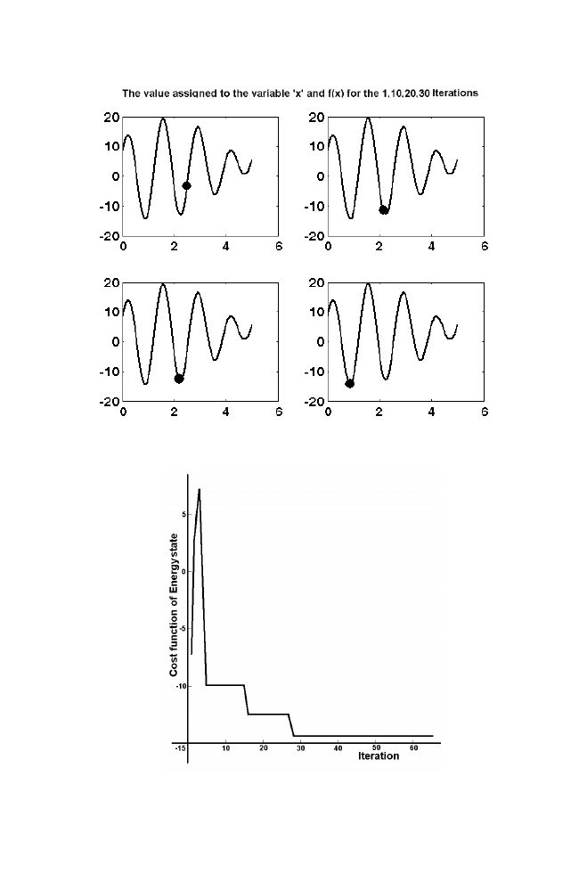
Initially the random value is selected within the range (0 to 5). Let the
selected value be 2.5 and the corresponding cost function is -3.4382. The
variable ‘curval’ is assigned the value 2.5 and the variable ‘curcost’ is
assigned the value -3.4382. Intialize the simulated temperature as T=1000.
Let the next randomly selected value be 4.9 and the corresponding cost
function is 3.2729. The variable ‘newval’ is assigned the value 4.9 and the
‘newcost’ is assigned the value 3.2729.
Note that ‘newcost’ value is higher than the ‘curcost’ value. As
‘newcost’> ‘curcost’, ‘newval’ is inferior compared with ‘curval’ in
minimizing the cost function. As the temperature (T) is large and
exp((curcost-newcost)/T)>rand, ‘newcost’ value is assigned to ‘curcost’ and
‘newval’ is assigned to ‘curval’. Now the temperature ‘T’ is reduced by the
factor 0.2171=1/log(100), where 100 is the number of iterations used. This is
the thumb rule used in this example. This process is said to one complete
iteration. Next randomly selected value is selected and the above described
process is repeated for 100 iterations.
The order in which the values are selected in the first 6 iterations is not
moving towards the local minima point which can be noted from the figure
1-6. This is due to the fact that the initial simulated temperature of the
annealing process is high.
The figure 1-6 shows all possible cost function values corresponding to
the ‘x’ values ranges from 0 to 5. The goal is to find the best value of x
corresponding to global minima of the graph given above. Note that the
global minima is approximately at x=0.8.
1. Artificial Intelligence
21
Figure1-7 Illustration of Simulated Annealing 1
As iteration increases the simulated temperature is decreased and the
value selected for the variable ‘x is moving towards the global minima point
as shown in the figure 1-7.
Thus values assigned to the variable ‘x’ for the first few iterations
(about 10 iterations in this example) is not really in decreasing order of
f(x). This helps to search the complete range and hence helps in
overcoming the problem of local minima. As iteration goes on increasing
the values selected for the variable ‘x’ is moving towards the global
minima which can be noted from the figure 1-8.
22 Chapter
1
Figure 1-8. Illustration of Simulated Annealing 2
Figure1-9. Illustration of Simulated Annealing 3

1. Artificial Intelligence
23
3.3
M-program for Simulated Annealing
___________________________________________________________
sagv.m
x=0:1/300:5
plot(x, minfcn(x))
hold
curval=rand*5;
curcost=minfcn(curval);
T=1000;
for i=1:1:100
newval=rand*5;
newcost=minfcn(newval);
if((newcost-curcost)<=0)
curval=newval;
curcost=minfcn(curval);
else
if(exp((curcost-newcost)/T)>rand)
curval=newval;
curcost=minfcn(curval);
end
end
T=T/log(100)
plot(curval,minfcn(curval),'r*');
CURRENTVAL{i}=curval;
M{i}=minfcn(curval);
pause(0.2)
end
___________________________________________________________
minfcn.m
function [res]=minfcn(x)
res=x+10*sin(5*x)+7*cos(4*x)+sin(x)
Matlab program for minimizing the function f(x)= x+10*sin(5*x)+
7*cos(4*x)+sin(x),where x varies from 0 to 5 .
24 Chapter
1
4.
BACK PROPAGATION NEURAL NETWORK
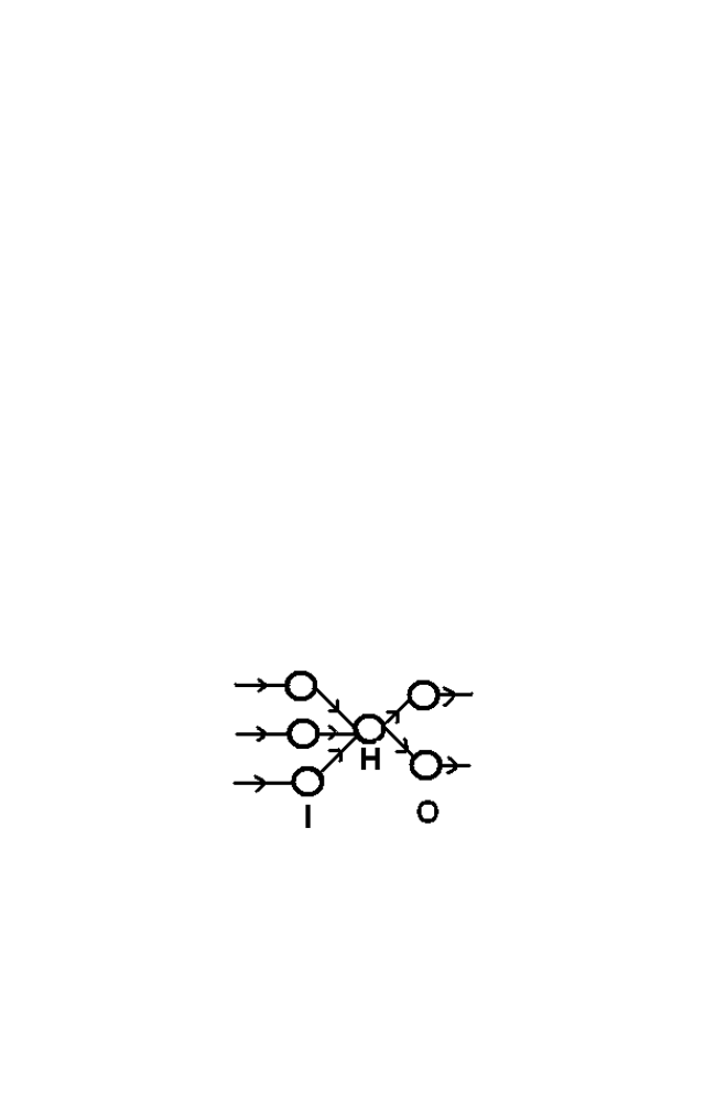
The model consists of layered architecture as shown in the figure 1-10.
Figure 1-10 BPN Structure
The mathematical model of the Biological Neural Network is defined as
Artificial Neural Network. One of the Neural Network models which are
used almost in all the fields is Back propagation Neural Network.
‘I’ is the Input layer ‘O’ is the output layer and ‘H’ is the hidden layer.
Every neuron of the input layer is connected to every neuron in the hidden
layer. Similarly every neuron in the Hidden layer is connected with every
neuron in the output layer. The connection is called weights.
Number of neurons in the input layer is equal to the size of the input
vector of the Neural Network. Similarly number of neurons in the output
layer is equal to the size of the output vector of the Neural Network. Size of
the hidden layer is optional and altered depends upon the requirement
For every input vector, the corresponding output vector is computed as
follows
[hidden vector] = func ([Input vector]*[Weight Matrix 1] + [Bias1 ])
[output vector] = func ([hidden vector]*[Weight Matrix 2] + [Bias2 ])
If the term [Input vector]*[Weight Matrix 1] value becomes zero, the
output vector also becomes zero. This can be avoided by using Bias vectors.
Similarly to make the value of the term ‘[Input vector]*[Weight Matrix 1] +
[Bias1]’ always bounded, the function ‘func’ is used as mentioned in the
equation given above.

1. Artificial Intelligence
25
___________
[1+exp(-x)]
tansig(x) = 2
_____________
[1+exp(-2x)]
The requirement is to find the common Weight Matrix and common Bias
vector such that for the particular input vector, computed output vector must
match with the expected target vector. The process of obtaining the Weight
matrix and Bias vector is called training.
Consider the architecture shown in the figure 1-9. Number of neurons in
the input layer is 3 and number of neurons in the output layer is 2. Number of
neurons in the hidden layer is 1.The weight connecting the i
th
neuron in the
first layer and j
th
neuron in the hidden layer is represented as W
ij
The weight
connecting i
th
neuron in the hidden layer and j
th
neuron in the output layer is
represented as W
ij
’ .
Let the input vector is represented as [i
1
i
2
i
3
]. Hidden layer output is
represented as [h
1
] and output vector is represented as [o
1
o
2
]. The bias
vector in the hidden layer is given as [b
h
] and the bias vector in the output
layer is given as [b
1
b
2
]. Desired ouput vector is represented is [t1 t2]
The vectors are related as follows.
h1=func1 (w
11
*i
1
+w
21
*i
2
+w
31
*i
3
+ b
h
)
o1= func2 (w
11
’*h
1
+b
1
)
o2= func2 (w
12
’*h
1
+b
2
)
t1~=o1
t2~=o2
4.1
Single Neuron Architecture
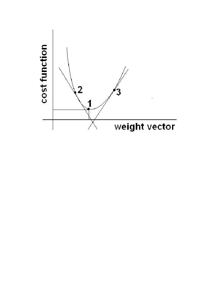
Consider the single neuron input layer and single neuron output layer.
Output= func (input * W +B)
Desired ouput vector be represented as ‘Target’
Requirement is to find the optimal value of W so that Cost function =
(Target-Output)
2
is reduced. The graph plotted between the weight vector
commonly Usually used ‘func’ are
logsig (x) = 1
‘W’ and the cost function is given in the figure 1-11.
Optimum value of the weight vector is the vector corresponding to the
point 1 which is global minima point, where the cost value is lowest.
26 Chapter
1
Figure 1-11 ANN Algorithm Illustration
The slope computed at point 2 in the figure is negative. Suppose if the
weight vector corresponding to the point 2 is treated as current weight vector
assumed, the next best value (i.e) global point is at right side of it. Similarly
if the slope is positive, next best value is left side of the current value. This
can be seen from the graph. The slope at point 3 is a positive. The best value
(i.e) global minimum is left of the current value.
Thus to obtain the best value of the weight vector. Initialize the weight
vector. Change the weight vector iteratively. Best weight vector is obtained
after finite number of iteration. The change in the weight vector in every
iteration is represented as ‘
ΔW’.
(i.e.) W (n+1) =W (n) +
ΔW (n+1)
W(n+1) is the weight vector at (n+1)
th
iteration W(n) is the weight vector
at n
th
iteration and
ΔW(n+1) is the change in the weight vector at (n+1)
th
iteration.
The sign and magnitude of the ‘
ΔW’ depends upon the direction and
magnitude of the slope of the cost function computed at the point
corresponding to the current weight vector.

1. Artificial Intelligence
27
Thus the weight vector is adjusted as following
New weight vector = Old weight vector -
μ*slope at the current cost value.
Cost function(C) = (Target-Output)
2
⇒ C= (Target- func (input * W +B))
2
Slope is computed by differentiating the variable C with respect to W and
is approximated as follows.
2((Target- func (input * W +B))* (-input)
=2*error*input
Thus W(n+1) =W(n) - 2*
μ*error*(-input)
⇒ W(n+1) = W(n) + γ error * input
This is back propagation algorithm because error is back propagated for
adjusting the weights. The Back propagation algorithm for the sample
architecture mentioned in figure 1-9 is given below.
4.2
Algorithm
Step 1: Initialize the Weight matrices with random numbers.
Step 2: Initialize the Bias vectors with random numbers.
Step 3: With the initialized values compute the output vector corresponding
to the input vector [i
1
i
2
i
3
] as given below. Let the desired target
vector be [t
1
t
2
]
h
1
=func1 (w
11
*i
1
+w
21
*i
2
+w
31
*i
3
+b
h
)
o
1
= func2 (w
11
’*h
1
+b
1
)
o
2
= func2 (w
12
’*h
1
+b
2
)
Step 4: Adjustment to weights
a) Between Hidden and Output layer.
w
11
’(n+1) = w
11
’(n) + γ
O
(t
1
-o
1
) *h
1
w
12
’(n+1) = w
12
’(n) + γ
O
(t
2
-o
2
) *h
1

28 Chapter
1
Note if momentum is included during training updating equations are
modified as follows.
w
11
’(n+1) = w
11
’(n) + γ
O
(t
1
-o
1
) *h
1
+
ρo * Δw
11
’(n)
Δw
11
’(n+1)
w
12
’(n+1) = w
12
’(n) +
Δw
12
’(n+1) +
ρo * Δw
12
(n)
w
11
(n+1) = w
11
(n) +
Δw
1
(n+1) +
ρ
H
*
Δw
11
(n)
w
21
(n+1) = w
21
(n) +
Δw
21
(n+1) +
ρ
H
*
Δw
21
(n)
b) Between Input layer and Hidden layer
w
11
(n+1) = w
11
(n) + γ
H
* e* i
1
w
21
(n+1) = w
21
(n) + γ
H
* e * i
2
w
31
(n+1) = w
31
(n) + γ
H
* e * i
3
‘e’ is the estimated error at the hidden layer using the actual error
computed in the output layer
(i.e.) e = h
1
* (1-h1)* [(t
1
-o
1
) + (t
2
-o
2
)]
Step 5: Adjustment of Bias
b
h
(n+1)= b
h
(n) +e* γ
H
b
1
(n+1) = b
1
(n) + (t
1
-o
1
)* γ
O
b
2
(n+1) = b
2
(n) + (t
2
-o
2
)* γ
O
Step 6: Repeat step 3 to step 5 for all the pairs of input vector and the
corresponding desired target vector one by one.
Step 7: Let d
1
, d
2
d
3
…d
n
be the set of desired vectors and y
1
, y
2
y
3
y
n
be the
corresponding output vectors computed using the latest updated
weights and bias vectors. The sum squared error is calculated as
SSE= (d
1
- y
1
)
2
+ (d
2
- y
2
)
2
+(d
3
- y
3
)
2
+(d
4
- y
4
)
2
+ … (d
n
- y
n
)
2
Step 8: Repeat the steps 3 to 7 until the particular SSE is reached.

1. Artificial Intelligence
29
w
31
(n+1) = w
31
(n) +
Δw
31
(n+1) +
ρ
H
*
Δw
31
(n)
b
h
(n+1)= b
h
(n) +e* γ
H +
ρ
H
*
Δb
h
(n)
Δ b
h
(n+1)
b
1
(n+1) = b
1
(n) +
Δ b
1
(n+1)
+
ρ
O
*
Δb
1
(n)
b
2
(n+1) = b
2
(n) +
Δ b
2
(n+1)
+
ρ
O
*
Δb
2
(n)
ρ
H
and
ρ
O
are the momentums used in the hidden and output layer
respectively.
4.3
Example
Consider the problem for training the Back propagation Neural Network
with Hetero associative data as mentioned below
Input
Desired Output
0 0 0 0 0
0 0 1 0 1
0 1 0 0 1
0 1 1 0 1
1 0 0 0 1
1 0 1 0 1
1 1 0 0 1
1 1 1 1 1
ANN Specifications
Number of layers = 3
Number of neurons in the input layer = 3
Number of neurons in the hidden layer =1
Number of neurons in the output layer = 2
Learning rate =0.01
Transfer function used in the hidden layer = ‘logsig’
Transfer function used in the output layer = ‘linear’ (i.e) output is taken as
obtained without applying non-linear function like ‘logsig’,’ tansig’.
30 Chapter
1
(See Figure 1-10)
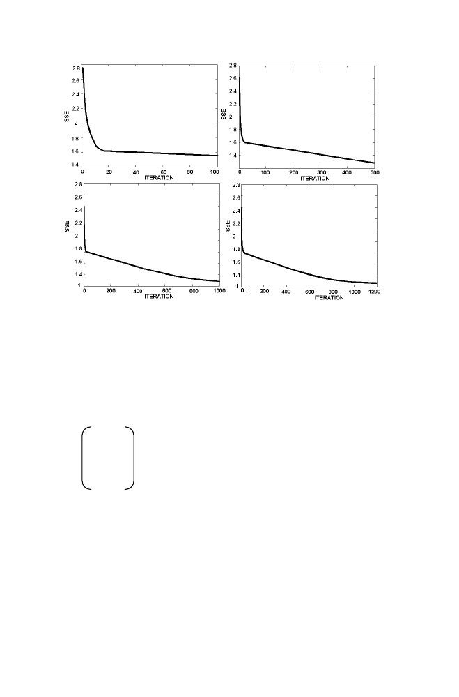
The Figure 1-12 describes how the Sum squared error is decreasing as
iteration increases. Note that sum squared error is gradually decreasing from
2.7656 as iteration increases and reaches 1.0545 after 1200 Iteration.
Trained Weight and Bias Matrix
W1 = 1.0374
0.9713
0.8236
B1= [-0.5526]
W2= [0.8499 1.3129]
B2= [-0.4466 -0.0163]
OUTPUT obtained after training the neural network
-0.1361 0.4632
0.0356 0.7285
0.0660 0.7756
0.2129 1.0024
0.0794 0.7962
Figure 1-12. Illustration of SSE decreases with Iteration

1. Artificial Intelligence
31
0.2225 1.0172
0.2426 1.0483
0.3244 1.1747
After rounding OUTPUT exactly matches with the Desired Output as shown
below
0 0
0 1
0 1
0 1
0 1
0 1
0 1
0 1
4.4
M-program for Training the Artificial Neural
Network for the Problem Proposed in the Previous
___________________________________________________________
anngv.m
SSE=[ ]; INDEX=[ ];
INPUT=[0 0 0;0 0 1;0 1 0;0 1 1;1 0 0;1 0 1;1 1 0;1 1 1];
DOUTPUT=[0 0;0 1;0 1 ;0 1;0 1;0 1;0 1 ;1 1];
W1=rand(3,1);W2=rand(1,2);
B1=rand(1,1); B2=rand(1,2);
for i=1:1:1200
for j=1:1:8
H=logsiggv(INPUT*W1+repmat(B1,[8 1]));
OUTPUT=H*W2 +repmat(B2,[8 1]);
ERR_HO=DOUTPUT - OUTPUT;
ERR_IH=H.*(1-H).*(sum(ERR_HO')');
lr_ho=0.01;
lr_ih=0.01;
W2(1,1)=W2(1,1)+ERR_HO(j,1)*H(j,1)*lr_ho;
W2(1,2)=W2(1,2)+ERR_HO(j,2)*H(j,1)*lr_ho;
W1(1,1)=W1(1,1)+ERR_IH(j,1)*INPUT(j,1)*lr_ih;
W1(2,1)=W1(2,1)+ERR_IH(j,1)*INPUT(j,2)*lr_ih;
W1(3,1)=W1(3,1)+ERR_IH(j,1)*INPUT(j,3)*lr_ih;
B1=B1+ERR_IH(j,1)*lr_ih;
B2(1,1)=B2(1,1)+ERR_HO(j,1)*lr_ho;
Section

32 Chapter
1
B2(1,2)=B2(1,2)+ERR_HO(j,2)*lr_ho;
end
INDEX=[INDEX i];
SSE=[SSE sum(sum(ERR_HO.^2))];
plot(INDEX,SSE,'r');
xlabel('ITERATION')
ylabel('SSE')
pause(0.2)
end
H=logsig(INPUT*W1+repmat(B1,[8 1]));
OUTPUT=H*W2 +repmat(B2,[8 1]);
______________________________________________________________________
logsiggv.m
function [res]=logsiggv(x)
res=1/(1+exp(-x));
5.
FUZZY LOGIC SYSTEMS
Monday, Tuesday, Wednesday, Thursday, Friday, and Saturday}. This is the
set in which elements belongs to the set with 100% membership.
Let us consider the set of rainy days ={Sunday (0.6), Monday (0.4),
Tuesday (0.4), Wednesday (0.6), Thursday (0.2), Friday (0.6), Saturday
(0.3)}. This is the set in which elements are associated with fuzzy
membership. Sunday (0.6) indicates that the Sunday belongs to the set of
rainy days with membership value 0.6. This is different from probability
assignment because in case of probability assignment, Sunday belongs to
non-rainy days with membership value 0.4. (ie) (1-0.6). But in case of fuzzy
sets Sunday belongs to non-rainy days with membership value of not
necessarily 0.4. It can be any value between 0 to 1.
5.1
Union and Intersection of Two Fuzzy Sets
Let us consider the example of computing union and intersection of fuzzy
sets as described below.
A={a (0.3), b (0.8), c (0.1), d (0.3)}
B={a (0.1), b (0.6), c (0.9), e (0-.1)}
Fuzzy is the set theory in which the elements of the set are associated with
fuzzy membership. Let us consider the set of days = {Sunday,
1. Artificial Intelligence
33
The elements of the set AUB are the unique elements collected from both
the sets A and B. The membership value associated with the elements of the
set AUB is the maximum of the corresponding membership values collected
from the set A and B.
Thus AUB = {a (0.3), b (0.8), c (0.9), d (0.3), e (0.1)}
Similarly the elements of the set A
∩B are the common elements
collected from the sets A and B. The membership value associated with the
elements of the set AUB is the minimum of the corresponding membership
values collected from the set A and B.
Thus
A
∩B= {a (0.1), b (0.6), c (0.1)}
5.2
Fuzzy Logic Systems
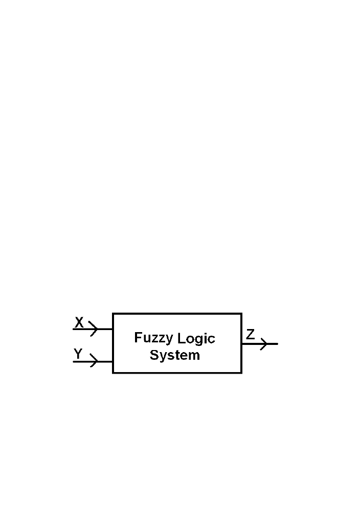
Let us consider the problem of obtaining the optimum value of the
variable ‘Z’ obtained as the output of the fuzzy logic system decided by the
values of the variable ‘X’ and ‘Y’ taken as the input to the fuzzy logic
system using fuzzy logic algorithm.
The values of the variable ‘X’ vary from X
min
to X
max.
Actual value of
min
to
X
max
is grouped into 3 sets XSMALL, XMEDIUM, XLARGE. The
relationship between the crisp value and fuzzy membership value is given in
the figure 1-13.
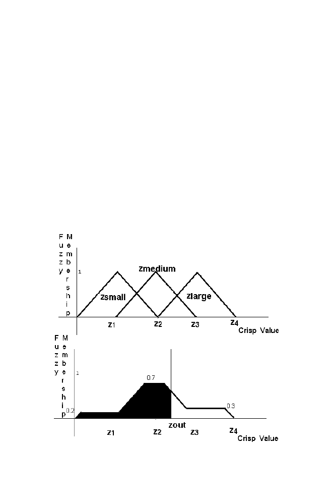
Figure 1-13. Fuzzy system
the variable is called crisp value. The group of the values ranges from X
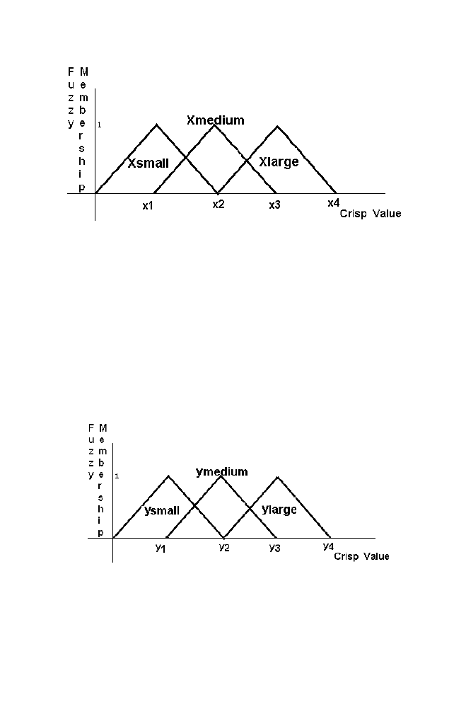
34 Chapter
1
Figure 1-14. Relaionship between crisp value and Fuzzy membership value for the variable X
The crisp values ranges from 0 to x2 belong to the set Xsmall. The crisp
values ranges from x1 to x3 belong to the set Xmedium. The crisp value
ranges from x2 to x4 belongs to the set Xlarge.
The crisp value from x1 to x2 of the Xsmall set and Xmedium set with
different membership value as mentioned in the Figure 1-14. Corresponding
membership value decreases gradually from 1 to 0 in the Xsmall set. But the
corresponding membership value increases gradually from 0 to 1 in the
Xmedium set.
Similarly the relationship between the crisp value and Fuzzy member
ship value for the variable ‘Y’ and the variable ‘Z’ are mentioned in the
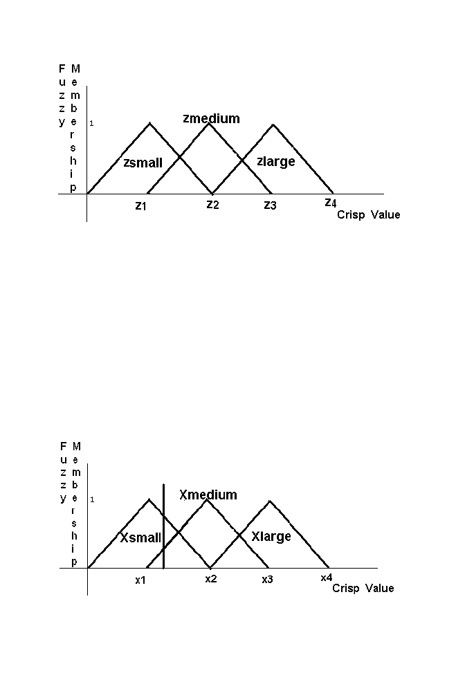
Figure 1-15 and Figure 1-16 respectively.
Figure 1-15. Relaionship between crisp value and Fuzzy membership value for the variable Y
1. Artificial Intelligence
35
Figure 1-16. Relaionship between crisp value and Fuzzy membership value for the variable Z
The identical relationship between the crisp value and fuzzy value of all
the variables X, Y and Z are chosen for the sake of simplicity (see figure).
Steps involved in obtaining the crisp value of the output variable for the
particular crisp values for the variable X and Y are summarized below.
5.2.1
Algorithm
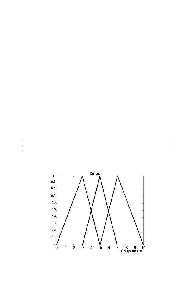
Step 1: Crisp to fuzzy conversion for the input variable ‘X’ and ‘Y’
Let us consider the crisp value of the input variable X be Xinput the crisp
value of the input variable Y be Yinput. Let Xinput belongs to the set
Xsmall with fuzzy membership 0.7 (say) belongs to set Xmedium 0.3 (say)
as shown in the Figure 1-17 and Figure 1-18 given below.
Figure 1-17. Xinput as the crisp input for the variable X
36 Chapter
1
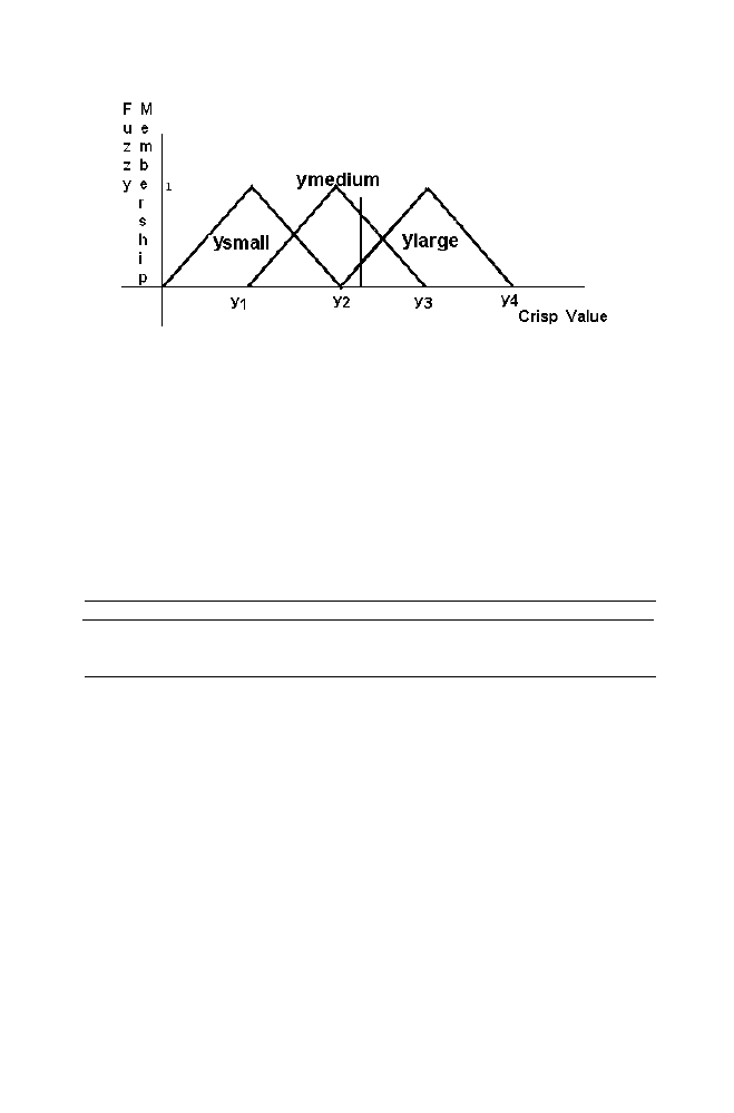
Similarly the Yinput belongs to the set Ymedium with fuzzy membership 0.7
and belongs to the set Ylarge with 0.2 as shown in the figure given below
Step 2: Fuzzy input to fuzzy output mapping using fuzzy base rule
Fuzzy base rule is the set of rules relating the fuzzy input and fuzzy output
of the fuzzy based system. Let us consider the Fuzzy Base Rule as shown in
the table given below.
Table 1-1. Fuzzy Base Rule
Ysmall Ymedium Ylarge
small
Zmedum Zmedium Zsmall
Xmedium
Zmedium Zlarge Zlarge
Xlarge
Zlarge Zlarge
Zmedium
Thus Fuzzy input set Xsmall = {Xinput (0.7) }
Xmedium = {Xinput (0.3) }
Xlarge = {Xlarge( 0 )
Ysmall = {Yinput (0) }
Ymedium = {Yinput (0.7) }
Ylarge = {Xlarge(0.2)
Fuzzy output set is obtained in two stages.
1. Intersection of Fuzzy sets
• Xsmall ∩ Ysmall = Zmedium ={Zoutput(0)}
• Xsmall ∩ Ymedium = Zmedium ={Zoutput(0.7)}
• Xsmall ∩ Ylarge = Zsmall ={Zoutput(0.2)}
• Xmedium ∩ Ysmall = Zmedium ={Zoutput(0)}
• Xmedium ∩ Ymedium = Zlarge={Zoutput(0.3)}
Figure 1-18. Yinput as the crisp input for the variable Y
1. Artificial Intelligence
37
• Xmedium ∩ Ylarge = Zlarge ={Zoutput(0.2)}
• Xlarge ∩ Ysmall = Zlarge ={Zoutput(0)}
• Xlarge ∩ Ymedium = Zmedium ={Zoutput(0)}
• Xlarge ∩ Ylarge = Zsmall ={Zoutput(0)}
2. Union of Fuzzy sets
• Zsmall = U(Zoutput(0.2), Zoutput(0))={ Zoutput(0.2) }
• Zmedium = U(Zoutput(0), Zoutput(0.7), Zoutput(0),Zoutput(0))
= {Zoutput (0.7)}
• Zlarge = U(Zoutput(0.3), Zoutput(0.2), Zoutput(0))={Zoutput(0.3)}
Thus Fuzzy output based on the framed fuzzy base rule is given as
Zsmall = {Zoutput(0.2)
Zmedium = {Zoutput(0.7}
Zlarge = {Zoutput(0.3)}
Step 3: Fuzzy to Crisp conversion for the output variable Z using
Centroid method
Figure 1-19. Defuzzification

38 Chapter
1
Truncate the portions of the Zsmall, Zmedium and Zlarge sections of the
output relationship above the corresponding thresholds obtained from output
fuzzy membership as shown in the figure. Remaining portions are combined
with overlapping of the individual sections. Combined sections can also be
obtained by adding the individual sections instantaneously as illustrated in
the example given in the section 5.4 Obtain the crisp value Zout which
divides the combined sections into two halves as shown in the figure. Thus
crisp value Zout is obtained for the corresponding input crisp value Xinput
and Yinput using Fuzzy logic system.
5.3
Why Fuzzy Logic System?
decide the output data. For example the automatic system is designed to
maintain the temperature of the water heater by adjusting the heat knob
based on the water level at that particular instant and temperature at that
particular instant. In this example water level measured using the sensor at
that particular instant and temperature measured using the sensor at that
particular instant are the input to the control system. Control system uses the
set of rules framed as given below for deciding the position of the heat knob
which is the output of the control system
• If T1<=Temperature <=T2 and W1<=Water level<=W2, Adjust the heat
knob position to K1. (Say).
• If T0<=Temperature <=T1 and W0<=Water level<=W1, Adjust the heat
knob position to K2. (Say) etc.
Suppose if the temperature is just less than T1, this rule is not selected.
The small variation ‘
ΔT’ makes the automatic control system not to select
this particular rule. To overcome this problem instead of using crisp value
for framing the rule, fuzzy values can be used to frame the rules (i.e) without
using the actual values obtained through input sensors This is called fuzzy
base rule as given below
• If the temperature of the water is small and water level is high, place the
heat knob in the high position. (say)
• If the temperature of the water is medium and water level is less, place
the heat knob in the less position. (say) etc.
The Automatic system uses set of rules framed with the input data to
1. Artificial Intelligence
39
In this case the problem only fuzzy sets are used for decision making which
makes the system to take decision like the human decision.
To design the fuzzy based system, the knowledge about the system
behavior is required to find the relationship between crisp value and the
fuzzy value (see above) and to frame the fuzzy base rule. This is the
drawback of the fuzzy based system when compared to ANN based system
which doesn’t require any knowledge about the system behavior.
5.4
Example
Let us consider the problem of obtaining the optimum value of the
variable ‘Z’ obtained as the output of the fuzzy logic system decided by the
values of the variable ‘X’ and ‘Y’ taken as the input to the fuzzy logic
system using fuzzy logic algorithm. The crisp –fuzzy relationship is as
mentioned in the section 5.2. The fuzzy base rule is as given in the table 1-1.
The values for the variables used in the section 5.2 are assumed as
mentioned in the table 1-2.
Table 1-2. Assumed values for the variables used in the section 5.2
X1 X2 X3 X4 Y1 Y2 Y3 Y4 Z1 Z2 Z3 Z4
3 5 7 10 20 45 65 100 35 70 90 100
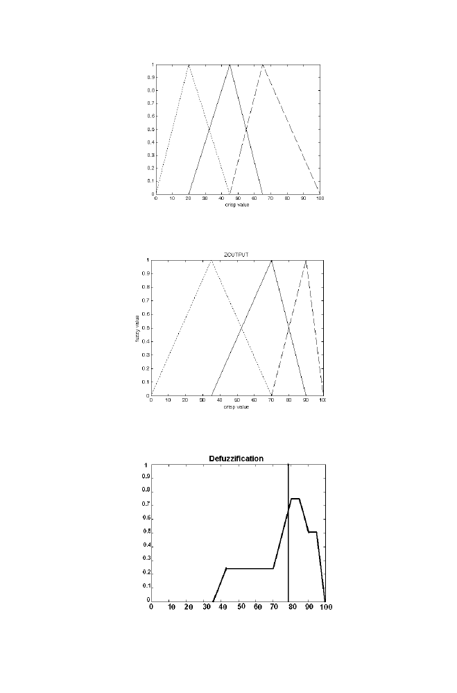
Figure 1-20. Relationship between crisp value and fuzzy membership for the Input variable X
For the arbitrary input crisp values xinput=6 and yinput=50, zout is obtained
as 78.8 using fuzzy logic system described in the section 5.2
in the example
40 Chapter
1
Figure1-21. Relationship between crisp value and fuzzy membership for the Input variable Y
Figure 1-22. Relationship between crisp value and fuzzy membership for the Input variable Z
Figure 1-23. Defuzzification in the example
in the example
in the example

1. Artificial Intelligence
41
5.5
M-program for the Realization of Fuzzy Logic
___________________________________________________________
fuzzygv . m
posx=[0 3 5 7 10];
maxx=max(posx);
posx=posx/max(posx);
posy=[0 20 45 65 100];
maxy=max(posy);
posy=posy/max(posy);
posz=[0 35 70 90 100];
maxz=max(posz);
posz=posz/max(posz);
i=posx(1):1/999:posx(2);
j=(posx(2)):(1/999):posx(3);
k=(posx(3)):(1/999):posx(4);
l=(posx(4)):(1/999):posx(5);
xsmall=[1/posx(2)*i (-1/(posx(3)-posx(2))*(j-posx(3))) zeros(1,length([k l]))];
xmedium =[zeros(1,length([i])) (1/(posx(3)-posx(2))*(j-posx(2))) (-1/(posx(4)-
posx(3))*(k-posx(4))) zeros(1,length([l]))];
xlarge=[zeros(1,length([i j])) (1/(posx(4)-posx(3))*(k-posx(3))) (-1/(posx(5)-posx(4))*(l-
posx(5))) ];
figure
plot([i j k l]*maxx,xsmall,':');
hold
plot([i j k l]*maxx,xmedium,'-');
plot([i j k l]*maxx,xlarge,'--');
xlabel('crisp value')
ylabel('fuzzy value')
title('XINPUT')
i=posy(1):1/999:posy(2);
j=(posy(2)):(1/999):posy(3);
k=(posy(3)):(1/999):posy(4);
l=(posy(4)):(1/999):posy(5);
ysmall=[1/posy(2)*i (-1/(posy(3)-posy(2))*(j-posy(3))) zeros(1,length([k l]))];
System for the Specifications given in Section 5.4

42 Chapter
1
ymedium =[zeros(1,length([i])) (1/(posy(3)-posy(2))*(j-posy(2))) (-1/(posy(4)-
posy(3))*(k-posy(4))) zeros(1,length([l]))];
ylarge=[zeros(1,length([i j])) (1/(posy(4)-posy(3))*(k-posy(3))) (-1/(posy(5)-posy(4))*(l-
posy(5))) ];
figure
plot([i j k l]*maxy,ysmall,':');
hold
plot([i j k l]*maxy,ymedium,'-');
plot([i j k l]*maxy,ylarge,'--');
xlabel('crisp value')
ylabel('fuzzy value')
title('YINPUT')
i=posz(1):1/999:posz(2);
j=(posz(2)):(1/999):posz(3);
k=(posz(3)):(1/999):posz(4);
l=(posz(4)):(1/999):posz(5);
zsmall=[1/posz(2)*i (-1/(posz(3)-posz(2))*(j-posz(3))) zeros(1,length([k l]))];
zmedium =[zeros(1,length([i])) (1/(posz(3)-posz(2))*(j-posz(2))) (-1/(posz(4)-
posz(3))*(k-posz(4))) zeros(1,length([l]))];
zlarge=[zeros(1,length([i j])) (1/(posz(4)-posz(3))*(k-posz(3))) (-1/(posz(5)-posz(4))*(l-
posz(5))) ];
figure
plot([i j k l]*maxz,zsmall,':');
hold
plot([i j k l]*maxz,zmedium,'-');
plot([i j k l]*maxz,zlarge,'--');
xlabel('crisp value')
ylabel('fuzzy value')
title('ZOUTPUT')
xinput=[6];
xinput=round(((xinput/maxx)*1000))
yinput=[50];
yinput=round(((yinput/maxy)*1000))
%fuzzy values
xfuzzy=[xsmall(xinput) xmedium(xinput) xlarge(xinput)];
yfuzzy=[ysmall(yinput) ymedium(yinput) ylarge(yinput)];

1. Artificial Intelligence
43
%Output fuzzy values obtained using framed fuzzy base rule
zfuzzys=max([(min([xfuzzy(1) yfuzzy(3)]))]);
zfuzzym=max([(min([xfuzzy(1) yfuzzy(2)])) (min([xfuzzy(2) yfuzzy(1)]))
(min([xfuzzy(3) yfuzzy(3)]))]);
zfuzzyl=max([(min([xfuzzy(2) yfuzzy(2)])) (min([xfuzzy(2) yfuzzy(3)])) (min([xfuzzy(3)
yfuzzy(1)])) (min([xfuzzy(3) yfuzzy(2)]))]);
%Defuzzification
zs=reshape((quantiz(zsmall,zfuzzys)*2-2)*(-
1/2),1,size(zsmall,2)).*zsmall+quantiz(zsmall,zfuzzys)'.*zfuzzys;
zm=reshape((quantiz(zmedium,zfuzzym)*2-2)*(-
1/2),1,size(zmedium,2)).*zmedium+quantiz(zmedium,zfuzzym)'.*zfuzzym;
zl=reshape((quantiz(zlarge,zfuzzyl)*2-2)*(-
1/2),1,size(zlarge,2)).*zlarge+quantiz(zlarge,zfuzzyl)'.*zfuzzyl;
figure
plot([i j k l]*maxz,zs,':')
hold
plot([i j k l]*maxz,zm,'-')
plot(zl,'--')
final=sum([zs;zm;zl]);
figure
plot([i j k l]*maxz ,final)
title('DEFUZZIFICATION')
S=cumsum(final)
[p,q]=find(S>=(sum(final)/2))
zout=(q(1)/1000)*maxz;
hold
plot(ones(1,100)*zout,[0:1/99:1],'*')
________________________________________________________________________
44 Chapter
1
6.
ANT COLONY OPTIMIZATION
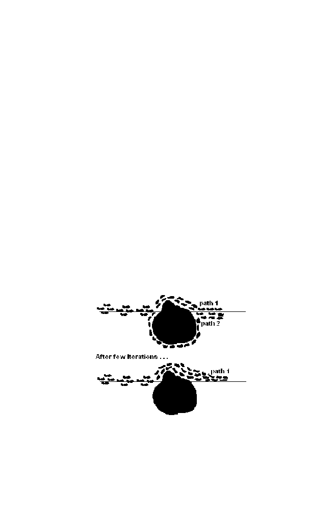
The figure 1-24 is the top view of the ants moving from source to
destination in search of food. There is the obstacle in the middle. There are
two paths available so that the ants can choose to move from source to
destination. As expected after some time duration ants prefer to choose
path1, which is the shortest distance between source and destination. This is
due to the fact that ants excrete the pheromones when they are moving. As
more ants have crossed the shortest path within the stipulated time when
compared to the other path, more pheromones are excreted in the shortest
path. This helps the following ants to choose the shortest path to cross the
obstacles.
The mathematical equivalent of this behavior is used in optimization
technique as the Ant colony optimization.
6.1
Algorithm
Consider the problem of finding the optimum order in which the numbers
from 1 to 8 are arranged so that the cost of that order is maximized. Cost of
the particular order is computed using the two matrices A and B as described
below.
Ant colony optimization techniques exploit the natural behavior of ants in
finding the shortest path to reach destination from the source.
Figure 1-24. Illustration of Ant Colony
1. Artificial Intelligence
45
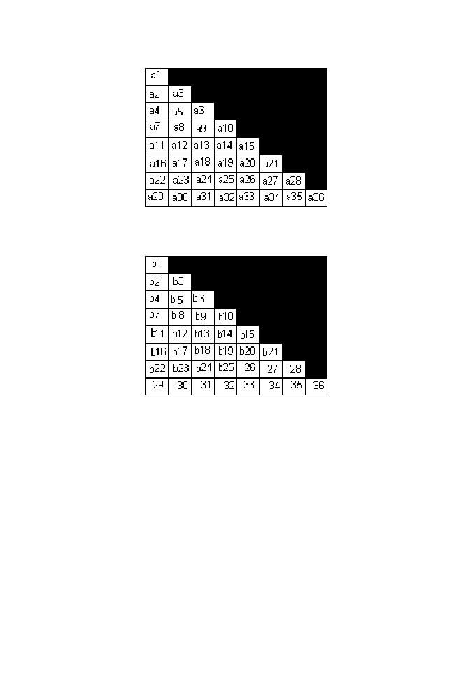
Figure 1-25. Matrix A
Figure 1-26. Matrix B
The cost of the order [3 2 1 5 7 2 4 6 8] is computed as the sum of the
product of values obtained from the positions (1,3) or (3,1), (2,2), (3,1), (4,5)
or (5,4) , (5,7) or (7,5) ,(6,2), (7,4) and (8,6) of the matrices A and B .
Cost ([3 2 1 5 7 2 4 6 8] ) =
a6*b6 + a3*b3 + a6*a6 + a14*b14 + a26*b26 +
a17*b17 +a25*b25 + a36*b36
(see Matrix A and Matrix B )
The problem of finding the optimal order is achieved using Ant colony
optimization technique as described below.
Step 1: Generate the 5 sets of orders randomly which are treated as the
initial values selected by the 5 Ants respectively.
The following are the orders selected by the 5 ants along with the
corresponding cost measured as described in the previous section.

46 Chapter
1
Table 1-3. Initialization of 5 values to the 5 Ants (say)
ANT ORDERS COST
ANT 1
7 1 3 6 2 5 4 8
C1
ANT 2
ANT 3
ANT 4
ANT 5
2 4 8 6 3 7 5 1
7 2 3 5 1 6 4 8
1 5 4 8 7 3 2 6
4 8 5 3 6 2 7 1
C2
C3
C4
C5
Pheromone matrix (n+1) = Pheromone matrix (n) + Updating Pheromone matrix
The value of the updating pheromone matrix must be high if the minimum
cost is assigned. Hence the matrix is filled up with the inverse values of the
corresponding cost as displayed below.
Table 1-4. Updating Pheromone Matrix
1 2 3 4 5 6 7 8
1 1/C4
1/C1
0
0 1/C3 0 0
1/C2+1/C5
2 1/C2
1/C3 0 0 1/C1
1/C5
1/C4 0
3 0 0
1/C1+1/C3
1/C5 1/C2 1/C4
0
0
4 1/C5
1/C2
1/C4 0 0 0
1/C1+1/C3
0
5
0 1/C4 1/C5 1/C3 0 1/C1 1/C2 0
6 0 0 0
1/C1+1/C2
1/C5 1/C3 0 1/C4
7
8
1/C1+1/C3
0
0
1/C5
0
1/C2
0
1/C4
1/C4
0
1/C2
0
1/C5
0
0
1/C1+1/C3
Step 2: Pheromone is the value assigned for selecting the i
th
number for the
j
th
position of the sequence selected by all the ants.(i.e) it is the
matrix in which the value at the index (i ,j) is the value assigned for
selecting the ith number for the jth position of the order selected by
all the ants. Initially the values of the matrix are completely filled up
with ones. The values of the Pheromone matrix are updated in every
iteration as

1. Artificial Intelligence
47
Let the order decided by the ant1 be represented as [u1 u2 u3 u4 u5 u6
u7 u8 ]
• The value for the u7 in the order as mentioned above is selected first as
the first number of the randomly generated position sequence is 7.
• To select the value for the u7, 7
th
column of the pheromone matrix is
used .(Note that 7
th
column belongs to 7
th
position of the order generated)
• 7
th
column of the pheromone matrix is rewritten below as Column7
vector arranged in row wise for better clarity.
Column7 = [0 1/C4 0 1/C1+1/C3 1/C2 0 1/C5 0]
• Normalized value of the 7
th
column of the pheromone matrix is given
below as Normalized vector7 arranged in row wise. This is also called as
the probability vector used for selecting the value for the u7 in the order.
S = [0 + 1/C4 + (1/C1+1/C3) + 1/C2 + 1/C5]
Normalized vector7 = (Column 7) / S = [p1 p2 p3 p4 p5 p6 p7 p8] (say)
Select the number corresponding to the position of the lowest value of the
normalized vector. Suppose if p5 is the lowest among the values in the
vector, the number 5 is assigned to the variable u7.
• The next value in the position sequence is 8.Hence the value for the
variable u8 is selected. But the value cannot be 5 as it was already
assigned to the variable u7. 8
th
column of the pheromone matrix except
the 5
th
row is used for selecting the value to be assigned to the variable u8
as described below.
• 8
th
column of the pheromone matrix is rewritten below as Column 8
vector with 5
th
row filled up X indicating 5
th
row is not consider for
selection. The vector is rearranged in row wise as displayed below
Column 8= [ (1/C2 +1/C5) 0 0 0 X 1/C4 0 (1/C1+1/C3) ]
• Normalized value of the 8
th
column of the pheromone matrix is
S= [(1/C2 +1/C5) + 0 + 0 + 0 + 1/C4 + 0 + (1/C1+1/C3)]
Normalized vector8 = (Column 8) / S = [q1 q2 q3 q4 q6 q7 q8]
Step 3: Next set of orders selected by the ants is as described below.
• Generate the position sequence randomly
7 8 2 3 6 4 1 5 (say)

48 Chapter
1
Select the number corresponding to the position of the lowest value of the
Normalized vector8. Suppose if q3 is the lowest among the values in the
vector, the number 3 is assigned to the variable u8.
This process is repeated to obtain the orders selected by the Ant 2, Ant3,
An4 and Ant 5.This is called one iteration.
Step 4:
• The updating pheromone matrix for the second iteration is computed as
described in the step 2 using the set of orders selected by the five ants in
the first iteration. This is called as Updating pheromone matrix (2).
• Pheromone matrix used in the 2
nd
iteration is computed as
Pheromone matrix (2) = Pheromone matrix (1) +Updating Pheromone matrix (2)
Note that best among the best set of orders selected by the five ants
in the last iteration is selected as the global best order.
6.2
Example
particular order is computed as described in the section 6.1. The matrices A and
B are given below.
A= 9 0 0 0 0 0 0 0 0
0 9 0 0 0 0 0 0 0
0 0 9 0 0 0 0 0 0
0 0 0 9 0 0 0 0 0
0 0 0 0 9 0 0 0 0
0 0 0 0 0 9 0 0 0
0 0 0 0 0 0 9 0 0
0 0 0 0 0 0 0 9 0
0 0 0 0 0 0 0 0 9
Consider the problem of finding the optimum order in which the numbers from
1 to 8 are arranged so that the cost of the order is maximized. Cost of the
Step 5: Next set of orders selected by the five ants are computed as
described in the step 3.
Step 6: The step 3 to step 5 is repeated for the particular number of
iterations. Thus best set of orders selected by the five ants are
obtained using Ant colony optimization.

1. Artificial Intelligence
49
B= 9 0 0 0 0 0 0 0 0
0 9 0 0 0 0 0 0 0
0 0 9 0 0 0 0 0 0
0 0 0 9 0 0 0 0 0
0 0 0 0 9 0 0 0 0
0 0 0 0 0 9 0 0 0
0 0 0 0 0 0 9 0 0
0 0 0 0 0 0 0 9 0
0 0 0 0 0 0 0 0 9
Initial orders selected by the four ants are displayed below.
ANT1: 5 4 2 1 3 6 7 8
ANT2: 3 7 8 5 2 1 4 6
ANT3: 5 1 7 2 4 3 6 8
ANT4: 6 1 7 2 8 5 3 4
Number of ants used to find the optimum order is 4. The orders selected
by the four ants after 50 Iterations are displayed below.
ANT1: 1 2 3 4 5 6 7 8
ANT2: 1 2 3 4 5 6 7 8
ANT3: 3 2 7 4 1 6 5 8
ANT4: 4 2 3 7 1 6 5 8
Note that ANT1 and ANT2 found the best order as expected using Ant
colony technique.
Initially the cost values are having more changes. After 40
th
iteration,
cost value gradually increases and reaches maximum which is the optimum
cost corresponding the optimum order selected using Ant colony
technique.
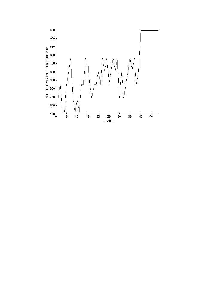
50 Chapter
1
Figure 1-27. Iteration (vs.) Best Cost selected by the 4 ants
6.3
M-program for Finding the
r the Specifications given in the
________________________________________________________
antcolonygv.m
%Consider the problem of finding the optimum order in which the numbers from 1 to 8
are
arranged
so
that
%the cost of that order is decreased .Cost of the particular order is computed using the
two matrices A and B as described below.
%The cost of the order [3 2 1 5 7 2 4 6 8] is computed as the sum of the product of
values
%obtained from the positions (1,3) or (3,1),(2,2),(3,1) ,(4,5) or (5,4) , (5,7) or (7,5) ,(6,2),
(7,4) and (8,6) of the matrices A and B .
%Cost ([3 2 1 5 7 2 4 6 8] ) = a6*b6 + a3*b3 + a6*a6 + a14*b14 + a26*b26 + a17*b17
+a25*b25 + a36*b36 see Matrix A and Matrix B
%Form the matrices given below
matA=diag([ones(1,9)*9]);
Optimal Order using Ant
Section 6.2
Colony Technique fo

1. Artificial Intelligence
51
matB=diag([ones(1,9)*9]);
%Initializing the orders selected by 4 Ants
[p1,ANT1]=sort(rand(1,8));
[p2,ANT2]=sort(rand(1,8));
[p3,ANT3]=sort(rand(1,8));
[p4,ANT4]=sort(rand(1,8));
%Intializing the Pheromone matrix
%columns are the positions
%rows are the value of the position
ANTS=[ANT1;ANT2;ANT3;ANT4];
P=ones(8,8);
col=[];
figure
hold
for i=1:1:50
%Updating pheromones
c1=computecost(ANTS(1,:),matA,matB);
c2=computecost(ANTS(2,:),matA,matB);
c3=computecost(ANTS(3,:),matA,matB);
c4=computecost(ANTS(4,:),matA,matB);
col=[col max([c1 c2 c3 c4])];
plot(col)
pause(0.01)
c=[c1 c2 c3 c4];
for i=1:1:8
for j=1:1:8
[x,y] = find(ANTS(:,i)==j);
for k=1:1:length(x)
P(j,i)=P(j,i)+(1/c(x(k)));
end
end
end
ANTS=[];
for i=1:1:4
P_cur=P;
tempant=zeros(1,8);
notation=[1 2 3 4 5 6 7 8];
[p,position]=sort(rand(1,8));

52 Chapter
1
for i=1:1:8
temp=P_cur(:,position(i));
temp=temp/sum(temp);
[value,index]=min(temp);
tempant(position(i))=notation(index);
P_cur(index,:)=[];
notation(index)=[];
end
ANTS=[ANTS;tempant];
end
c1=computecost(ANTS(1,:),matA,matB);
c2=computecost(ANTS(2,:),matA,matB);
c3=computecost(ANTS(3,:),matA,matB);
c4=computecost(ANTS(4,:),matA,matB);
end
_____________________________________________________________
computecost.m
function
[s]=computecost(A,P,Q)
s=0;
for
i=1:1:8
s=s+P(max(i,A(i)),min(i,A(i))).*Q(max(i,A(i)),min(i,A(i)));
end

Chapter 2
PROBABILITY AND RANDOM PROCESS
Algorithm Collections
1.
INDEPENDENT COMPONENT ANALYSIS
combination of ‘n’ independent signals x
1
(t) , x
2
(t) … x
n
(t) , where n>=m is
given below.
y
1
(t) = a
11
x
1
(t) + a
12
x
2
(t) + a
13
x
3
(t) + …a
1n
x
n
(t)
y
2
(t) = a
21
x
1
(t) + a
22
x
2
(t) + a
23
x
3
(t) + …a
2n
x
n
(t)
y
3
(t) = a
31
x
1
(t) + a
32
x
2
(t) + a
33
x
3
(t) + …a
3n
x
n
(t)
y
4
(t) = a
41
x
1
(t) + a
42
x
2
(t) + a
43
x
3
(t) + …a
4n
x
n
(t)
…
y
m
(t) = a
m1
x
1
(t) + a
m2
x
2
(t) + a
m3
x
3
(t) + …a
mn
x
n
(t)
Independent signals are obtained from the mixed signals using
Independent Component Analysis (ICA) algorithm as described below
1.1
ICA for Two Mixed Signals
The samples of the signals x
1
(t) and x
2
(t) are represented in the vector
form as x
1
=[x
11
x
12
x
13
…x
1n
] and x
2
=[x
21
x
22
x
23
… x
2n
] respectively. The
signals y
1
(t)=a
11
*x
1
(t)+a
12
*x
2
(t) and y
2
(t)=a
21
*x
1
(t)+a
22
*x
2
(t) are represented
in the vector form as y
1
=[y
11
y
12
y
13
…y
1n
] and y
2
=[y
21
y
22
y
23
… y
2n
]
Consider ‘m’ mixed signals y
1
(t), y
2
(t)…y
m
(t) obtained from the linear
53
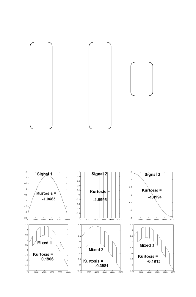
54 Chapter
2
respectively. Thus the ICA problem can be represented in the form of matrix
as described below.
y
11
y
21
x
11
x
21
y
12
y
22
x
12
x
22
y
13
y
23
x
13
x
23
y
14
y
24
x
14
x
24
a
11
a
21
y
15
y
25
x
15
x
25
y
16
y
26
=
x
16
x
26
a
12
a
22
.
.
.
y
1n
y
2n
x
1n
x
2n
[Y]
T
= [X]
T
[A]
T
Given the matrix [Y], obtaining the matrices [X] and [A] such that the
columns of the matrix [X]
T
are independent to each other is the ICA problem.
Consider three independent signals and the corresponding mixed signals
along with the kurtosis values are displayed below.

2. Probability and Random Process
55
Kurtosis is the statistical parameter used to measure the Gaussian nature
of the signal. Kurtosis is inversely proportional to the Gaussianity of the
signal. Note that the kurtosis values are maximum for independent signals
compared to the mixed signals. (i.e.) Independent signals are more non-
Gaussian compared with mixed signals. Mathematically kurtosis is
computed using the formula as displayed below, where E[X] is the
expectation of the vector X
ICA problem is to obtain the matrices [X] and [A] such that column
vectors of the matrix [X]
T
are independent to each other. (i.e.) Kurtosis
values computed for the column vectors are maximum.
[Y]
T
= [X]
T
[A]
T
( i.e.) [Y] = [A] [X]
[X] = [A]
-1
[Y]
[X]=[B][Y]
X1 and X2 are the two column vectors of the matrix [X]
T
(i.e.) [X]
T
= [X1 X2]
Kurtosis measured for the Column vector [X1] is given as
E [X1
4
]-3{E [X1
2
]}
2
Similarly kurtosis measured for the column vector [X2] is given as
E [X2
4
]-3{E [X2
2
]}
2
56
Estimating the best values for the matrix [B] such that kurtosis measured
for the column vectors of the matrix [X]
T
= [[B][Y]]
T
as defined above is
maximum
We require another constraint about the matrix [B] to obtain the values of
the matrix [B] which is described below
The covariance matrix (COV(Y)) computed for the group of vectors
collected row-by-row of the matrix Y
T
is computed using the formula as
displayed below
Let M = (y
11
+ y
12
+y
13
+…y
1n
) / n
(y
21
+ y
22
+y
23
+…y
2n
) / n
COV(Y) =
y
11
y
11
y
21
+ y
12
y
12
y
22
+ … y
1n
y
1n
y
2 n
/n
-
MM
T
y
21
y
22
y
2n
(i.e) COV(Y) = E[YY
T
] - MM
T
The matrix computed is of size 2x2. The value at the position (1,1)
conveys the information about how the first elements of the collected vectors
are correlated with itself (variance). The value at the position (1,2) conveys
the information about how the first elements are correlated with second
elements of the collected vectors.
For example the covariance matrix computed for 2D vectors collected
from the particular independent signals and the corresponding mixed signals
are given below.
COV
independent
=
0.2641 x 10
-006
-0.1086 x 10
-006
-0.1086 x 10
-006
0.5908 x 10
-006
COV
mixed
= 0.1086 0.0613
0.0613 0.0512
Chapter
2

2. Probability and Random Process
57
To compare the covariance matrix, correlation coefficient is used. It is the
normalized covariance matrix whose (m, n) element is computed as
COV( m, n) / (sqrt(COV(m,m)*COV(n,n))
The correlation co-efficient for the above covariance matrix (COV) is given
below
CORR
independent
= 1 -0.2750
-0.2750 1
CORR
mixed
= 1
0.822
0.822 1
Note that cross correlation value is less for independent signals compared to
the mixed signals. This fact is used as the source for second constraint. (i.e.)
the correlation coefficients matrix of the independent signals is almost
identity matrix. Also if the variances of the signals are unity the covariance
matrix and the correlation co-effients are identical.
The mean and variance of the mixed signals are made 0 and 1 respectively
so that the mean and variance of the row vectors of the matrix [Y] are 0 and
1 respectively. [Refer Mean and variance Normalization Section 4 of
Chapter 2]
The matrix [Y] can be transformed into another matrix [Z] such that the
covariance matrix computed for the 2D vectors collected from the matrix [Z]
as described above is almost unit vector (diagonal) using KLT (Refer
Hotelling transformation). (i.e.) E[[Z][Z]
T
]=[I]
Let us define the transformation matrix [T], which transforms the matrix
[Y] into [Z] as described below.
[Z]=[T][Y] implies
[Y]=[T]
-1
[Z] implies
[Y]=[U] [Z]
Also, [X]=[B][Y]

58
[X]=[B][U][Z]
[B][U][Z]=[X]
[B][U][B][B]
-1
[Z]=[X]
[A][Z]={[B][U][B]}
-1
[X]
Note that A=[B]
-1
Column vectors of the transformation matrix [U] are orthonormal to
each other. (ie) [U]
T
= [U]
-1
If E [XX
T
] = [I] (Identity Matrix)
((i.e.) Covariance matrix of the Independent signals with mean zero and
variance one is Identity matrix )
Computing Covariance Matrix of the RHS of the equation
[A][Z]={[B][U][B]}
-1
[X]
E [({[B][U][B]}
-1
[X]) ({[B][U][B]}
-1
[X])
T
]
= E [({[B][U][B]}
-1
)
[X] [X]
T
({[B][U][B]}
-1
)
T
]
= ({[B][U][B]}
-1
) E [XX
T
] ({[B][U][B]}
-1
)
T
= ({[B][U][B]}
-1
) ({[B][U][B]}
-1
)
T
= ([B]
-1
[U]
-1
[B]
-1
) ( [B]
-1
[U]
-1
[B]
-1
)
T
=[B]
-1
[U]
-1
[B]
-1
[B
-1
]
T
[U
-1
]
T
[B
-1
]
T
Chapter
2

2. Probability and Random Process
59
If the columns of the B matrix is orthonormal to each other
( i.e.) [B]
-1
= [B]
T
[B]
-1
[U]
-1
[B]
-1
[B
-1
]
T
[U
-1
]
T
[B
-1
]
T
=[B]
-1
[U]
-1
[U
-1
]
T
[B
-1
]
T
= [B]
-1
[B
-1
]
T
(Because [U]
T
=[U]
-1
)
=[B]
-1
[B]
= [I] (Identity Matrix )
Computing Covariance Matrix of the LHS of the equation
[A][Z]={[B][U][B]}
-1
[X]
E (([A][Z]) ([A][Z])
T
)
=AE[ZZ
T
]A
T
= [A][I][A]
T
= [B]
-1
[B
-1
]
T
= [I]
(Because [B]
-1
=[B]
T
is assumed )
Thus Covariance matrix of the LHS and RHS are Identity matrix if
• E[XX
T
] is the Identity matrix (Assumed)
• E[ZZ
T
] is the Identity matrix (Property)
• [B]
-1
= [B]
T
(Assumed)
• [U]
-1
=[U]
T
(Property)
60
In other words, If the Columns of the matrix [B] are orthonormal to each
other (i.e) [B]
-1
= [B]
T
, then E[XX
T
]=[I] (i.e) Covariance Matrix of the
independent signals is the Identity Matrix.(Required).
[A][Z]={[B][U][B]}
-1
[X]
When [A] is estimated such that covariance matrix of the LHS and RHS are
Identity Matrix, [A][Z]=[X] (ie) {[B][U][B]}
-1
becomes the Identity matrix.
Thus ICA Problem is the optimization problem as mentioned below.
Given the matrix [Y], estimating the best values for the matrix [B] such
that kurtosis measured for the row vectors of the matrix [X]
=
[A][Z]=[B
T
][Z] is maximum.
Subject to the constraint B
T
B=[I] (i.e) column vectors of the matrix B is
orthonormal to each other.
Let [B] = b
11
b
12
b
21
b
22
Z = z
11
z
12
z
13
… z
1n
z
21
z
22
z
23
… z
2n
[B]
T
[Z] = b
11
b
21
z
11
z
12
z
13
… z
1n
b
12
b
22
z
21
z
22
z
23
… z
2n
= b
11
z
11
+b
21
z
21
b
11
z
12
+b
21
z
22
… b
11
z
1n
+b
21
z
2n
b
12
z
11
+b
22
z
21
b
12
z
12
+b
22
z
22
… b
12
z
1n
+b
22
z
2n
Kurtosis of the first row = E[(b
11
z
1i
+b
21
z
2i
)
4
] – 3 {E[(b
11
z
1i
+b
21
z
2i
)
2
]}
2
Kurtosis of the second row= E[(b
12
z
1i
+b
22
z
2i
)
4
] – 3 {E[(b
12
z
1i
+b
22
z
2i
)
2
]}
2
Chapter
2

2. Probability and Random Process
61
Constraint [B]
T
[B]=[I ]
(i.e ) b
11
b
11
+b
21
b
21
=1
b
12
b
12
+b
22
b
22
=1
Thus Iterative approach to estimate the best values for B matrix using
Lagrange’s method is described below.
Partial differentiating the function
E[(b
11
z
1i
+b
21
z
2i
)
4
] – 3 {E[(b
11
z
1i
+b
21
z
2i
)
2
]}
2
+
λ (b
11
b
11
+b
21
b
21
–1)
with respect to the unknown constants b
11,
b
21
and equate to zero.
With respect to b
11
E[4(b
11
z
1i
+b
21
z
2i
)
3
z
1i
]-3 *2{E[(b
11
z
1i
+b
21
z
2i
)
2
]}E[2(b
11
z
1i
+b
21
z
2i
) z
1i
]
+
λ*2*b
11
=0
E[(b
11
z
1i
+b
21
z
2i
)
2
] is the variance of the independent signal. This can be
assumed to be 1.
Also E (z
1i
z
1i
) is the variance of the first mixed signal and hence it is 1. E
(z
1i
z
2i
) is the covariance between the two mixed signals and the value is
zero.
Therefore the above equation becomes
4*E[(b
11
z
1i
+b
21
z
2i
)
3
z
1i
]-6*2 *b
11
+
λ*2*b
11
=0
Let the Lagrange multiplier
λ be (-2). [For More Details Refer
Estimation Techniques]
Thus Iteration equation becomes
b
11
(t+1) = E[(b
11
(t)z
1i
+b
21
(t)
z
2i
)
3
z
1i
]-3*b
11
(t)
b
11
(t) is the value for b
11
in t
th
iteration
b
11
(t+1) is the value for b
11
in (t+1)
th
iteration
Similarly iteration equation for other elements of the matrix B are
computed and are displayed below

62
b
11
(t+1) = E[(b
11
(t)z
1i
+b
21
(t)
z
2i
)
3
z
1i
]-3*b
11
(t)
b
21
(t+1) = E[(b
11
(t)z
1i
+b
21
(t)
z
2i
)
3
z
2i
]-3*b
21
(t)
b
12
(t+1) = E[(b
12
(t)z
1i
+b
22
(t)
z
2i
)
3
z
1i
]-3*b
12
(t)
b
22
(t+1) = E[(b
12
(t)z
1i
+b
22
(t)
z
2i
)
3
z
2i
]-3*b
22
(t)
Recall that the columns of the matrix B are made orthonormal to each
other. This can be explicitly performed in every iteration, after updating the
values using the equation given above.
1.1.1
ICA algorithm
Chapter
2
Step 1: Given mixed signals y1(t) and y2(t) are converted into z1(t) and
z2(t) using Hotellilng transformation such that the covariance matrix
computed using the converted signals z1(t) and z2(t) is the identity
matrix.[Use Hotelling Transformation]
Step 2: Initialize the values for the matrix B such that B
T
B=[I]
Step 3: Update the elements of the matrix B using the Iteration formula
displayed above.
Step 4: Columns of the matrix B is made orthonormal to each other as
mentioned below.
B = B * real(inv(B' *B)^(1/2));
Step 5: Repeat step 3 and step 4 for ‘N’ Iteration.
Step 6: Independent signals are obtained by multiplying B
T
with the Z
matrix
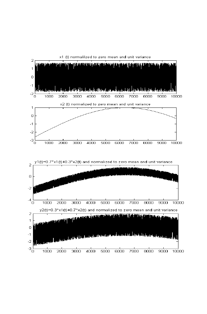
2. Probability and Random Process
63
Example: Independent signals x1 (t) and x2 (t) are mixed to get the
signals y1 (t)=0.3*x1 (t)+0.7*x2 (t), y2 (t)=0.7*x1 (t)+0.3*x2 (t) as shown
in the figure given below
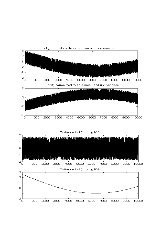
64
Using ICA independent signals are obtained in two stages with
decorrelated signals z1(t) and z2(t) in the first stage and the Independent
estimated signals x1(t) and x2(t) in the second stage as displayed below.
Number of Iterations (N) used is 10000.
Chapter
2

2. Probability and Random Process
65
1.2
M-file for Independent Component Analysis
___________________________________________________________
icagv.m
%ICA WITH THREE COMPONENTS
close all
clear all
i=0:1/10:1000;
a=sin(0.1*pi*i);
a=a(1:1:10000);
a=meanvarnorm(a,0,1)
b=randn(1,10000);
b=meanvarnorm(b,0,1);
i=0:1/10:1000;
c=exp(0.001*pi*i);
c=meanvarnorm(c,0,1);
c=c(1:1:10000);
s1=0.9*a+0.6*b+0.6*c;
s1=meanvarnorm(s1,0,1);
s2=0.6*a+0.9*b+0.6*c;
s2=meanvarnorm(s2,0,1);
s3=0.6*a+0.6*b+0.9*c;
s3=meanvarnorm(s3,0,1);
figure
subplot(3,1,1)
plot(a);
subplot(3,1,2)
plot(b);
subplot(3,1,3)
plot(c);
figure
subplot(3,1,1)
plot(s1);
subplot(3,1,2)
plot(s2);
subplot(3,1,3)
plot(s3);
%ICA START
data1=[s1;s2;s3];
MEANMAT=repmat(mean(data1')',1,length(data1));

66
c1=cov(data1');
[T1,E1]=eig(c1);
data2=T1'*(data1-MEANMAT);
%data2=T1*(data1);
c2=cov(data2');
[T2,E2]=eig(c2);
data=E2^(-1/2)*data2;
T=E2^(-1/2)*T1;
c=cov(data');
figure
subplot(3,1,1)
plot(data(1,:));
subplot(3,1,2)
plot(data(2,:));
subplot(3,1,3)
plot(data(3,:));
%ICA STARTS
w11=rand(1);
w12=rand(1);
w13=rand(1);
w21=rand(1);
w22=rand(1);
w23=rand(1);
w31=rand(1);
w32=rand(1);
w33=rand(1);
W1=[w11 w21 w23]';
W2=[w12 w22 w32]';
W3=[w13 w23 w33]';
W=[W1 W2 W3]';
W = W * real(inv(W' * W)^(1/2));
w11=W(1,1);
w12=W(1,2);
w13=W(1,3);
w21=W(2,1);
w22=W(2,2);
w23=W(2,3);
w31=W(3,1);
w32=W(3,2);
w33=W(3,3);
for i=1:1:40000
w11=sum(((w11*data(1,:)+w21*data(2,:)+w31*data(3,:)).^3).*data(1,:))/length(data);
Chapter
2

2. Probability and Random Process
67
w21=sum(((w11*data(1,:)+w21*data(2,:)+w31*data(3,:)).^3).*data(2,:))/length(data);
w31=sum(((w11*data(1,:)+w21*data(2,:)+w31*data(3,:)).^3).*data(3,:))/length(data);
w12=sum(((w12*data(1,:)+w22*data(2,:)+w32*data(3,:)).^3).*data(1,:))/length(data);
w22=sum(((w12*data(1,:)+w22*data(2,:)+w32*data(3,:)).^3).*data(2,:))/length(data);
w32=sum(((w12*data(1,:)+w22*data(2,:)+w32*data(3,:)).^3).*data(3,:))/length(data);
w13=sum(((w13*data(1,:)+w23*data(2,:)+w33*data(3,:)).^3).*data(1,:))/length(data);
w23=sum(((w13*data(1,:)+w23*data(2,:)+w33*data(3,:)).^3).*data(2,:))/length(data);
w33=sum(((w13*data(1,:)+w23*data(2,:)+w33*data(3,:)).^3).*data(3,:))/length(data);
w11=w11-3*w11;
w12=w12-3*w12;
w13=w13-3*w13;
w21=w21-3*w21;
w22=w22-3*w22;
w23=w23-3*w23;
w31=w31-3*w31;
w32=w32-3*w32;
w33=w33-3*w33;
W1=[w11 w21 w23]';
W2=[w12 w22 w32]';
W3=[w13 w23 w33]';
W=[W1 W2 W3]';
W = W * real(inv(W' *W)^(1/2));
w11=W(1,1);
w12=W(1,2);
w13=W(1,3);
w21=W(2,1);
w22=W(2,2);
w23=W(2,3);
w31=W(3,1);
w32=W(3,2);
w33=W(3,3);
W*W';
end
W=[w11 w12 w13;w21 w22 w23;w31 w32 w33];
y=W'*data;
figure
subplot(3,1,1)
plot(y(1,:));
subplot(3,1,2)
plot(y(2,:));
subplot(3,1,3)
plot(y(3,:));

68
2.
GAUSSIAN MIXTURE MODEL
Let us consider the data collected from the certain group of people about
their age and height are represented in two-dimensional vectors. Let the first
element of the vector be the age and the second element is the height of the
corresponding person, as described below. P
1
= [a
1
h
1
], P
2
= [a
2
h
2
] ... P
m
=
[a
m
h
m
]. Now let us define the problem for classifying the collected group of
vectors into ‘n’ category called as ‘n’ clusters, such that the centroids of the
clusters are away from each other and the data belonging to the same cluster
are nearer to each other as shown in the figure. The dots in the Figure 2-1
belong to the centroid of the individual clusters. The problem defined is
called clustering the data, otherwise called as grouping the data.
Let us model the probability of the particular vector ‘x’ from the
collected data as the Linear combination of Multi Variate Gaussian density
function.
(ie) p(x) = p(c
1
) * Gaussian density function of ‘x’ with mean vector
‘m
1
’ and covariance matrix ‘cov
1
’ + p(c
2
) * Gaussian density function of ‘x’
with mean vector ‘m
2
’ and covariance matrix ‘cov
2
’ + … p(c
n
) * Gaussian
density function of ‘x’ with mean vector ‘m
n
’ and covariance matrix ‘cov
n
’
where p(c
n
) is the probability of the clustern n.
The model described above is called as Gaussian Mixture Model. Given
such that the probability of the collected data is maximized is the task to be
performed for modeling. As the collected data are independent to each other,
the probability of the collected data (p) is represented as the product of p(x
1
),
p(x
2
)…p(x
m
) (ie) P
D
=p(x
1
) p(x
2
)…p(x
m
)
Chapter
2
(ie) p(x) = p(c
1
) p(x/c
1
) + p(c
2
) p(x/c
2
) + p(c
3 )
p(x/c
3
) +. . . p(c
n
)
p(x/c
n
)
the data (x
1
, x
2,
x
3,
x
4…
x
m
) , obtaining the mean vectors m
1
, m
2
, … and the
covariance matrices c
1
, c
2
, … and the probability of clusters p(c
1
), p(c
2
)…

2. Probability and Random Process
69
Figure 2-1. Clustering Example with Four Clusters
Estimating the best values for mean vectors and covariance matrices such
that the probability P
D
is maximized is described below.
m
1
= [(p(c
1
/x
1
)*(x
1
) + p(c
1
/x
2
)*(x
2
)+ p(c
1
/x
3
)*(x
3
)+…… p(c
1
/x
m
)*x
m
)]
______________________________________________________
p(c
1
/x
1
)+ p(c
1
/x
2
)+ p(c
1
/x
3
)+…… p(c
1
/x
m
)
where p (c
1
/x
1
) is computed as [p(x
1/
c
1
) * p (c
1
)] / [p(x
1
)]
Note that p(x
1/
c
1
) is the probability of ‘x
1’
computed using Gaussian
density function of ‘x’ with mean ‘m
1
’ and covariance ‘cov
1
’. Also p(x
1
) =
p(c
1
) p(x
1
/c
1
) + p (c
2
) p(x
1
/c
2
) + p(c
3 )
p(x
1
/c
3
) + . . . p(c
n
) p(x
1
/c
n
)
Maximization is obtained by differentiating P
D
= P
D
=p(x
1
) p(x
2
)…p(x
m
)
with respect to the unknown parameters m
1
, m
2
, m
3
, … m
n
, cov
1
, cov
2
,
cov
3
…cov
n
and equate to zero. Solving the above set of obtained equations
gives the best estimate of the unknown parameters, which are listed below

70
The requirement is to estimate the best value for m1.But for computing
the best value requires p(c
1
/x
1
), which in further requires p(x
1/
c
1
) as discussed
above. p(x1/c1) requires m1 for computation. [Surprise!].
To proceed further, an iteration approach called as Expected –
Maximization algorithm is used to estimate the best value for m
1
as
described below.
2.1
Expectation-maximization Algorithm
Chapter
2
1. Initialize the mean vectors randomly m
1
, m
2
, m
3,
… m
n
2. Find the Euclidean distance between the x
1
vector and the mean vectors
m
1
m
2 …
m
n
are computed as ‘d1’, ‘d2’, … ‘dn’ respectively. If the
distance d2 is smaller among all, the x
1
vector is treated as the vector
belongs to the 2
nd
cluster. In general if the dk is smallest among all, x
1
vector belongs to the k
th
cluster. Thus cluster index assigned to the vector
x
1
is ‘k’. Similarly cluster index is obtained for the entire data vector.
3. Let the number of data belongs to the first cluster be ‘k’. (ie) Number of
data vectors having cluster index 1 is ‘k. Then p (c1) = probability of the
cluster 1 is computed as
p (c
1
) = k1
________________
Total Number of data
and p(c2) is computed as
p (c
2
) = k2
________________
Total Number of data
and so on
4. Covariance matrix of the cluster 1 is computed as cov
1
= E ([X-
μ
X
]
[X-
μ
X
T
]) = E (XX
T
)-
μ
X
μ
X
T
. For instance, let us consider the vectors x
1,
x
3
,
x
7
, and x
9
arranged in the column format, belongs to cluster1 and the
corresponding covariance matrix is computed as follows.
μ
X
= [x
1
+ x
3
+ x
7
+x
9
]/4.
E (XX
T
) = [x
1
x
1
T
+ x
2
x
2
T
+ x
3
x
3
T
+ x
4
x
4
T
]/4
Thus cov
1
is computed as E (XX
T
) -
μ
X
μ
X
T
.
5. Similarly, the covariance matrices cov
2
, cov
3
, cov
4 …
cov
n
are computed.

2. Probability and Random Process
71
2.1.1
Expectation Stage
Using the above initialized values,
[ p (c
1
/x
1
), p (c
1
/x
2
) p (c
1
/x
3
)… p (c
1
/x
m
)
p (c
2
/x
1
), p (c
2
/x
2
) p (c
2
/x
3
)… p (c
2
/x
m
)
p (c
3
/x
1
), p (c
3
/x
2
) p (c
3
/x
3
)… p (c
3
/x
m
)
p (c
4
/x
1
), p (c
4
/x
2
) p (c
4
/x
3
)… p (c
4
/x
m
)
…
p (c
n
/x
1
), p (c
n
/x
2
) p (c
n
/x
3
)… p (c
n
/x
m
)]
are computed. This is called Expectation stage of the E-M algorithm.
2.1.2
Maximization stage
Maximization stage of the E-M algorithm belongs to maximizing the
probability P
D
. That is obtained by differentiating the probability P
D
with
respect to unknown parameter and equating them to zero. Solving the set of
obtained equations gives the best estimate of unknown parameters which are
listed below.
[(p(c
1
/x
1
)*(x
1
) + p(c
1
/x
2
)*(x
2
)+ p(c
1
/x
3
)*(x
3
)+…… p(c
1
/x
m
)*x
m
)]
m
1
= ____________________________________________________
p(c
1
/x
1
)+ p(c
1
/x
2
)+ p(c
1
/x
3
)+…… p(c
1
/x
n
)
[(p(c
1
/x
1
)*(x
1
) + p(c
1
/x
2
)*(x
2
)+ p(c
1
/x
3
)*(x
3
)+…… p(c
1
/x
m
)*x
m
)]
m
2
= ____________________________________________________
p(c
1
/x
1
)+ p(c
1
/x
2
)+ p(c
1
/x
3
)+…… p(c
1
/x
n
)
[(p(c
1
/x
1
)*(x
1
) + p(c
1
/x
2
)*(x
2
)+ p(c
1
/x
3
)*(x
3
)+…… p(c
1
/x
m
)*x
m
)]
m
3
= ____________________________________________________
p(c
1
/x
1
)+ p(c
1
/x
2
)+ p(c
1
/x
3
)+…… p(c
1
/x
n
)
[(p(c
1
/x
1
)*(x
1
) + p(c
1
/x
2
)*(x
2
)+ p(c
1
/x
3
)*(x
3
)+…… p(c
1
/x
m
)*x
m
)]
m
4
= ____________________________________________________
p(c
1
/x
1
)+ p(c
1
/x
2
)+ p(c
1
/x
3
)+…… p(c
1
/x
n
)
[(p(c
n
/x
1
)*( [x
1
-
μ
X1
] [x
1
-
μ
X1
]
T
) + …… p(c
n
/x
m
)* ( [x
m
-
μ
Xm
] [x
m
-
μ
Xm
]
T
)]
cov
n
= ____________________________________________________________
p(c
n
/x
1
)+ p(c
n
/x
2
)+ p(c
n
/x
3
)+…… p(c
n
/x
m
)

72
The computed values are the current best estimates of means and
covariance matrices. Using this Expectation stage is executed, followed by
Maximization stage. Thus Expectation stage and Maximization stage is
repeated for N iterations and hence best estimate of the means and
covariance matrices are obtained using E-M algorithm.
Using the estimated means p(c
1
), p(c
2
), p(c
3
)…p(c
n
) are obtained and
hence the Gaussian Mixture Model of the collected is obtained.
2.2
Example
Two dimensional vectors are randomly generated and the Gaussian
Mixture Model of the generated data is obtained using the algorithm
described above is displayed below.
About 350 vectors are randomly generated. Among which 100 vectors
are with mean [0.9 0.8], 100 vectors are with mean [0.7 0.6] and 150 vectors
are with mean [0.5 0.4].
The elements of the individual vector are generated independently and
hence the estimated covariance matrices are diagonal in nature.
Estimated values of the GMM model after 10 Iterations are given below
Mean vector 1 = [0.9124 0.7950]
Mean vector 2 = [0.7125 0.6091]
Mean vector 3 = [0.4994 0.3990]
Covariance matrix 1
0.0045 -0.0001
-0.0001 0.0047
Covariance matrix 2
0.0048 -0.0003
-0.0003 0.0048
Covariance matrix 3
0.0055 -0.0005
-0.0005 0.0054
Chapter
2

2. Probability and Random Process
73
2.3
Matlab Program
___________________________________________________________
gmmmodelgv.m
%GMM MODEL
cluster1=clustercol([0.9 0.8],100);
cluster2=clustercol([0.7 0.6],100);
cluster3=clustercol([0.5 0.4],150);
clustertot=[cluster1 cluster2 cluster3];
%[p,q]=kmeans(clustertot',3);This may be used for initializing the means
q(1,:)=[0.83 0.79];
q(2,:)=[0.76 0.74];
q(3,:)=[0.6 0.3];
%To Estimate q ,cov1,cov2,cov3
[p]=clusterno(clustertot,q);
[m1,n1]=find(p==1);
collect1=clustertot(:,n1);
if(length(n1)~=0)
cov1=cov(collect1');
else
cov1=diag([1 1]);
end
[m1,n1]=find(p==2);
collect2=clustertot(:,n1);
cov2=cov(collect2');
if(length(n1)~=0)
cov2=cov(collect2');
else
cov2=diag([1 1]);
end
[m1,n1]=find(p==3);
collect3=clustertot(:,n1);
cov3=cov(collect3');
if(length(n1)~=0)
cov3=cov(collect3');
else
cov3=diag([1 1]);
end
plot(collect1(1,:),collect1(2,:),'r*')

74
hold on
plot(collect2(1,:),collect2(2,:),'g*')
hold on
plot(collect3(1,:),collect3(2,:),'b*')
hold on
pause(0.3)
w1=length(find(p==1))/length(p);
w2=length(find(p==2))/length(p);
w3=length(find(p==3))/length(p);
for j=1:1:10
pw1x=[];
pw2x=[];
pw3x=[];
for i=1:1:length(clustertot)
pw1x=[pw1x (w1*pxw(clustertot(:,i),q(1,:),cov1))/...
(w1*pxw(clustertot(:,i),q(1,:),cov1)+...
w2*pxw(clustertot(:,i),q(2,:),cov2)+...
w3*pxw(clustertot(:,i),q(3,:),cov3))];
pw2x=[pw2x (w2*pxw(clustertot(:,i),q(2,:),cov2))/...
(w1*pxw(clustertot(:,i),q(1,:),cov1)+...
w2*pxw(clustertot(:,i),q(2,:),cov2)+...
w3*pxw(clustertot(:,i),q(3,:),cov3))];
pw3x=[pw3x (w3*pxw(clustertot(:,i),q(3,:),cov3))/...
(w1*pxw(clustertot(:,i),q(1,:),cov1)+...
w2*pxw(clustertot(:,i),q(2,:),cov2)+...
w3*pxw(clustertot(:,i),q(3,:),cov3))];
end
q(1,1)=sum(pw1x.*clustertot(1,:))/sum(pw1x);
q(1,2)=sum(pw1x.*clustertot(2,:))/sum(pw1x);
q(2,1)=sum(pw2x.*clustertot(1,:))/sum(pw2x);
q(2,2)=sum(pw2x.*clustertot(2,:))/sum(pw2x);
q(3,1)=sum(pw3x.*clustertot(1,:))/sum(pw3x);
q(3,2)=sum(pw3x.*clustertot(2,:))/sum(pw3x);
cov1(1,1)=sum(pw1x.*[(clustertot(1,:)-q(1,1)).*...
(clustertot(1,:)-q(1,1))])/sum(pw1x);
cov1(1,2)=sum(pw1x.*[(clustertot(1,:)-q(1,1)).*...
(clustertot(2,:)-q(1,2))])/sum(pw1x);
cov1(2,1)=sum(pw1x.*[(clustertot(2,:)-q(1,2)).*...
(clustertot(1,:)-q(1,1))])/sum(pw1x);
cov1(2,2)=sum(pw1x.*[(clustertot(2,:)-q(1,2)).*...
(clustertot(2,:)-q(1,2))])/sum(pw1x);
Chapter
2

2. Probability and Random Process
75
cov2(1,1)=sum(pw2x.*[(clustertot(1,:)-q(2,1)).*...
(clustertot(1,:)-q(2,1))])/sum(pw2x);
cov2(1,2)=sum(pw2x.*[(clustertot(1,:)-q(2,1)).*...
(clustertot(2,:)-q(2,2))])/sum(pw2x);
cov2(2,1)=sum(pw2x.*[(clustertot(2,:)-q(2,2)).*...
(clustertot(1,:)-q(2,1))])/sum(pw2x);
cov2(2,2)=sum(pw2x.*[(clustertot(2,:)-q(2,2)).*...
(clustertot(2,:)-q(2,2))])/sum(pw2x);
cov3(1,1)=sum(pw3x.*[(clustertot(1,:)-q(3,1)).*...
(clustertot(1,:)-q(3,1))])/sum(pw3x);
cov3(1,2)=sum(pw3x.*[(clustertot(1,:)-q(3,1)).*...
(clustertot(2,:)-q(3,2))])/sum(pw3x);
cov3(2,1)=sum(pw3x.*[(clustertot(2,:)-q(3,2)).*...
(clustertot(1,:)-q(3,1))])/sum(pw3x);
cov3(2,2)=sum(pw3x.*[(clustertot(2,:)-q(3,2)).*...
(clustertot(2,:)-q(3,2))])/sum(pw3x);
[p]=clusterno(clustertot,q);
w1=length(find(p==1))/length(p);
w2=length(find(p==2))/length(p);
w3=length(find(p==3))/length(p);
[m1,n1]=find(p==1);
collect1=clustertot(:,n1);
[m1,n1]=find(p==2);
collect2=clustertot(:,n1);
[m1,n1]=find(p==3);
collect3=clustertot(:,n1);
close all
plot(collect1(1,:),collect1(2,:),'r*')
hold on
plot(q(1,1),q(1,2),'co')
plot(collect2(1,:),collect2(2,:),'g*')
plot(q(2,1),q(2,2),'mo')
plot(collect3(1,:),collect3(2,:),'b*')
plot(q(3,1),q(3,2),'yo')
pause(0.3)
totcol1{j}=collect1;
totcol2{j}=collect2;
totcol3{j}=collect3;
qcol{j}=q;
end
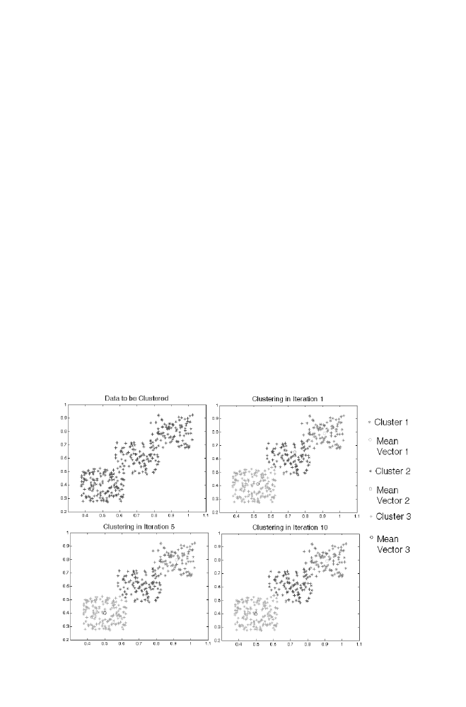
76
___________________________________________________________
clustercol.m
function [res] =clustercol(pos,N)
x1=rand(1,N)/4-(0.25)/2;
y1=rand(1,N)/4-(0.25)/2;
res=[x1+pos(1);y1+pos(2)];
_______________________________________________________________________
clusterno.m
function [q]=clusterno(clustertot,q)
d1=(clustertot'-repmat(q(1,:),length(clustertot),1)).^2;
d1=sum(d1');
d2=(clustertot'-repmat(q(2,:),length(clustertot),1)).^2;
d2=sum(d2');
d3=(clustertot'-repmat(q(3,:),length(clustertot),1)).^2;
d3=sum(d3');
[p,q]=min([d1;d2;d3]);
________________________________________________________________________
2.4
Program Illustration
Chapter
2

2. Probability and Random Process
77
3.
K-MEANS ALGORITHM FOR PATTERN
RECOGNITION
If the groups of n-dimensional vectors are given, there is the need to classify
the vectors into ‘k’ category. The centroid vectors of each group are used to
represent the identity for ‘k’ category. (i.e) If the new vector is to be
classified among the ‘k’ category, the distance between the new vector with
all the centroids are computed. The centroid corresponding to the smallest
distance is treated as the identified group. The centroids of all the groups are
obtained using K-means algorithm as described below.
Consider the set of normalized marks (i.e. the mark ranges from 0 to 1)
scored by the 100 students in the class for particular subject. Each mark is
treated as the vector with one-dimensional. There is the need to classify the
collected marks into 6 groups for allocating 6 grades. This is done using k-
means algorithm as described below.
3.1
K-means Algorithm
3.2
Example
The particular sets of marks (data) are subjected to k-means algorithm Final
clusters along with clusters obtained at every iteration are displayed below.
Note that after 6
th
iteration, clusters are not changed.
Step 1: Initialize the 6 centroids randomly corresponding to 6 grades .
Step 2: Classify the marks and identify the grade for the individual marks
using the initialized 6 centroids as described in the section 3.
Step 3: Find the mean of the marks collected in the particular grade say ‘1’.
This is treated as the centroid corresponding to the grade 1 used for
the next iteration. This process is repeated to compute the new sets
of centroids corresponding to the individual grade.
Step 4: Go to step 2.
Step 5: The process involved from Step 2 to Step 4 is considered as the one
iteration and this process is repeated for finite number of iterations to
obtain the final centroids corresponding to each grades.

78
Figure 2-2. Illustration of K-Means Algorithm
Figure 2-3
.
Data along with the final centroids obtained by k-means algorithm
In the above-mentioned example, the data ranges from 0.0067 to 0.9925
and the six centroids obtained in the 10
th
iteration are displayed below.
0.0743 0.2401 0.4364 0.6115 0.7763 0.9603 (see the Figure 2-3).
3.3
Matlab Program for the K-means Algorithm
Applied for the Example given in Section 3.2
kmeansgv.m
________________________________________________________________________
a=rand(1,100);
plot(a,zeros(1,100),'*');
b=rand(1,6);
for iter=1:1:10
hold off
M=[(a-b(1)).^2;(a-b(2)).^2;(a-b(3)).^2;(a-b(4)).^2;(a-b(5)).^2;(a-b(6)).^2;];
[P,CLUSTERNO]=min(M);
u=['r','g','b','c','m','y'];
figure
Chapter
2

2. Probability and Random Process
79
for i=1:1:6
[x,y]=find(CLUSTERNO==i);
col=[];
for k=1:1:length(x)
col= [col a(x(k),y(k))];
end
plot(col,zeros(1,length(col)),strcat(u(i),'*'))
hold on
b(i)=mean(col);
end
pause(0.01)
end
________________________________________________________________________
4.
FUZZY K-MEANS ALGORITHM FOR PATTERN
RECOGNITION
Consider the problem described in the section 3 for classifying the
normalized marks into 6 clusters for the assignment of grades.
In fuzzy k-means technique, fuzzy set theory is used to obtain the optimal
values of the centroid.
In this technique the particular vector (In this problem it is the
normalized mark scored by the student) belongs to all the 6 clusters with
different membership values. For instant the vector 0.3 belongs to the
different clusters with different membership values as given below
Cluster 1 = {0.3 (0.0001)}
Cluster 2 = {0.3 (0.0448)}
Cluster 3 = {0.3 (0.0022)}
Cluster 4 = {0.3 (0.0031)}
Cluster 5 = {0.3 (0.9492)}
Cluster 6 = {0.3 (0.0007)}
The numbers in bold letters are the corresponding membership values.
(i.e.) 0.3 belongs to the cluster 1 with membership value 0.0001 and belongs
to the cluster 2 with membership value 0.0448 and so on. Note that sum of
the membership values is 1.

80
Consider the vector x1 belongs to the cluster 1 whose centroid is c1, then
(x1-c1)^2 must be minimized. But if the x1 belongs to cluster 1 with the
membership value m1, then m1*(x1-c1)^2 has to be minimized. Similarly x1
belongs to the cluster 2 whose centroid is c2. Also x1 belongs to the cluster 2
with membership value m2. Thus the term m2*(x1-c2)^2 also has to be
minimized.
Thus the fuzzy k-means problem is treated as the optimization technique
for obtaining the membership values along with the centroids of the
individual clusters such that
100 6
Σ
Σ
M
ik
2 *
(x
i
-c
k
)
2
is minimized
i=1 k=1
M
ij
is membership value of the vector xi belongs in the cluster k. Xi is the
i
th
vector. c
k
is the k
th
centroid.
The algorithm for obtaining the centroids along with membership values
is displayed below.
4.1
Fuzzy K-means Algorithm
M
11 =
1/
[((vector 1-c1)
2
/ (vector1 –c1)
2
)
2
+
((vector 1-c1)
2
/ (vector1 –c2
2
)
2
+
((vector 1-c1)
2
/ (vector1 –c3
2
)
2
+
((vector 1-c1)
2
/ (vector1 –c4
2
)
2
+
((vector 1-c1)
2
/ (vector1 –c5
2
)
2
+
((vector 1-c1)
2
/ (vector1 –c6
2
)
2
]
Chapter
2
Step 1: Intialize the membership values (M
ij
) randomly.
Step 2: Compute the centroids of the 6 clusters.
C1=[Vector1* (the member ship value of the vector 1 belongs to the
cluster 1)
2
(i.e.) M
11
2
+ Vector2* (the member ship value of the vector 2
belongs to the cluster 1)
2
(i.e.) M
12
2
+… Vector100* (the member ship
value of the vector 100 belongs to the cluster 1)
2
(i.e.) M
1,100
2
]/
Sum of the squared values of the membership values belonging to the
cluster 1.
Similarly the centroids C2, C3, C4, C5 and C6 are obtained.
Step 3: Update the membership values M using the current values of the 6
centroids as given below.

2. Probability and Random Process
81
M
45 =
1/
[((vector 4-c5)
2
/ (vector4 –c1)
2
)
2
+
((vector 4-c5)
2
/ (vector4–c2
2
)
2
+
((vector 4-c5)
2
/ (vector4 –c3
2
)
2
+
((vector 4-c5)
2
/ (vector4 –c4
2
)
2
+
((vector 4-c5)
2
/ (vector4 –c5
2
)
2
+
((vector 4-c5)
2
/ (vector4 –c6
2
)
2
]
Similarly other membership values are computed.
4.2
Example
The particular sets of marks (data) are subjected to Fuzzy k-means
algorithm. Final clusters along with clusters obtained at every iteration are
displayed below.
Figure
2
-4. Illustration of Fuzzy K-means algorithm
Step 4: Compute the sum of the squared difference between the previous
membership value and the current membership value. If the computed
value is not less than the threshold value go to step 2 to compute the
next set of centroids and followed by next set of membership values. If
the threshold value is less than the threshold value, stop the iteration.
Thus the centroids are obtained using fuzzy k-means algorithm. Using
the computed centroids, clustering can be obtained as described in the
section 3.
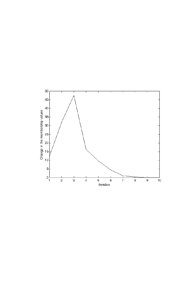
82
Figure 2-5. Data and the final centroids obtained using Fuzzy k-means algorithm
In the above mentioned example data ranges from 0.0099 to 0.9883.
The final centroids obtained after 10 iteration using fuzzy k-means
algorithm is displayed below 0.0313 0.2188 0.3927 0.5317 0.6977
0.8850 (see figure 2-5). Also the graph between the sum of the squared
difference between the previous membership value and the current
membership value (vs.) Iteration number is displayed below.
Figure 2-6. Illustration of change in the membership value in every iteration
Chapter
2

2. Probability and Random Process
83
4.3
Matlab Program for the Fuzzy k-means Algorithm
Applied for the Example given in the Section 4-2
___________________________________________________________
fuzzykmeansgv.m
%Fuzzy k-means algorithm
a=rand(1,100);
s=[];
fm=[];
for i=1:1:100
r=rand(1,6);
r=r/sum(r);
fm=[fm;r];
end
%Computation of centroids using fuzzy membership
for l=1:1:10
for i=1:1:6
cen{i}=sum((fm(:,i).^2).*a')/sum(fm(:,i).^2);
end
%Updating fuzzy membership value (fm)
fm1=[];
for p=1:1:6
for q=1:1:100
temp=0;
for r=1:1:6
temp =temp+(((a(q)-cen{p})^2)/((a(q)-(cen{r}))^2))^2;
end
fm1(q,p)=1/temp;
end
end
s=[s sum(sum((fm-fm1).^2))];
fm=fm1;
b=cell2mat(cen);
M=[(a-b(1)).^2;(a-b(2)).^2;(a-b(3)).^2;(a-b(4)).^2;(a-b(5)).^2;(a-b(6)).^2;];
[P,CLUSTERNO]=min(M);
u=['r','g','b','c','m','y'];
figure
for i=1:1:6
[x,y]=find(CLUSTERNO==i);
col=[];

84
for k=1:1:length(x)
col= [col a(x(k),y(k))];
end
plot(col,zeros(1,length(col)),strcat(u(i),'*'))
hold on
end
pause(0.01)
end
figure
plot(s)
xlabel('Iteration')
ylabel('Change in the membership values
5.
MEAN AND VARIANCE NORMALIZATION
Suppose in the speech recognition system the two speech signals
corresponding to the same word are to be compared. Two signals are not
recorded exactly with the same volume (i.e.) the two signals are not with the
same energy. Thus before extracting features from the speech signals, there
is the need to normalize the speech signal in terms of mean and variance so
that two speech signals are made recorded with the same volume.
Mean and variance normalization of the signal is obtained as described
below. Consider the speech signal ‘A(t)’ with mean ‘m
d
’ and variance ‘v
d
’
and speech signal ‘B(t)’ with mean m and variance ‘v’. The requirement is to
normalize the speech signal B(t) so that the mean and variance are changed
to the desired mean ‘m
d
’ and desired variance ‘v
d
’ respectively. The
procedure for the mean and variance normalization is given below.
5.1
Algorithm
Let
Δ
i
be the value calculated for the i
th
sample of the signal ‘A’
(original signal) and is computed as described below.
Chapter
2
Step 1: Create the vector completely filled up desired mean ‘m
d
’. Number of
elements of the vector is equal to the number of samples in the
speech signal.
Step 2: Each and every element of the vector is added with +
Δ or -Δ. If the
sample value in the original vector is greater than mean ‘m’, add +
Δ
to the corresponding sample in the vector created. Otherwise the
value is added with ‘-
Δ’. The value of the ‘Δ’ is computed using the
sample value, mean ‘m’, variance ‘v’ of the signal ‘A (t)’ and the
desired variance ‘v
d
’ .
___________________________________________________________
2. Probability and Random Process
85
The value A (i) is deviated from ‘m’ with (A (i)-m) when the standard
deviation of the signal is v
(1/2)
, then the deviation of the signal from the
desired mean ‘m
d
’ with the standard deviation of the signal v
d
(1/2)
is given by
Δ
i
=(v
d
/v)
(1/2)
*(A(i)-m)
5.2
Example 1
Consider the speech signal A(t) with mean=0.0062 and variance=0.0057
which is kept as the reference signal. Consider speech signal
B(t) corresponding to the same word with mean=0.0061 and
variance=0.0094. The speech signal B(t) is subjected to mean and variance
normalization as described above to obtain B(t) with desired mean and
variance as shown in the figure below.
Figure
2
-7. Illustration of Mean and Variance Normalization of the speech signal

86
Note that the signal at the top and the bottom of the figure 2-7 are almost
identical. This preprocessing stage is normally used before extracting
features from the signal for pattern recognition.
5.3
M-program for Mean and Variance Normalization
________________________________________________________
meanvarnormgv.m
%a is the speech signal to be modified
%b is the reference signal with desired mean and variance.
% res is the normalilzed version of signal ‘a’ with desired mean and variance
m=mean(a);
v=sqrt(var(a));
md=mean(b);
vd=sqrt(var(b));
delta=abs((a-m)*vd/v);
res=ones(1,length(a))*md;
[p]=quantiz(a,m);
p=p'; p=p*2-1;
res=res+p.*delta;
________________________________________________________________________
Chapter
2

Chapter 3
NUMERICAL LINEAR ALGEBRA
Algorithm Collections
1.
HOTELLING TRANSFORMATION
Consider the set of n-dimensional vectors collected in which the elements of
the vector are dependent to each other (i.e.) the covariance matrix computed
for the collected vectors are not the diagonal matrix. The co-variance matrix
is computed as follows.
co-variance matrix is computed using E[(X-µ
x
) (X-µ
x
)
T
] = E(XX
T
)- µ
x
µ
x
T
,
where µ
x
is the mean vector computed using the collected vectors (ie)
µ
x
=[x
1
+x
2
+x
3
+…x
m
]/m.
Hotelling Transformation transforms the set of vectors x
1
, x
2
,…x
m
into
computed for the transformed vectors is diagonal in nature.
Covariance Matrix (CM)
a
1
b
1
c
1
d
1
b
1
b
2
c
2
d
2
c
1
c
2
c
3
d
3
d
1
d
2
d
3
d
4
Let x
1
, x
2
,…x
m
be the collection of ‘m’, ‘n-dimensional vectors. The
another set of vectors (ie) y
1
, y
2
,…y
m
, such that the covariance matrix
87

88 Chapter
3
The element a
1
in the above matrix gives the information about how the
first elements of the collected vectors are correlated to each other. Similarly
c
1
gives the information about how the first elements are correlated with
third element. Thus if the matrix is the diagonal matrix, then the elements of
the vectors collected are made independent to each other.
1.1
Diagonalization of the Matrix ‘CM’
1. Compute the Eigen values and the corresponding Eigen vectors of the
matrix ‘CM’
Number of Eigen values obtained is equal to the size of the matrix. For
instance the size of the above mentioned matrix is 4 and hence number of
Eigen values = 4. Let it be
λ
1
,
λ
2
,
λ
3
and
λ
4
2. Compute the Eigen vector ‘X
1
’corresponding to the Eigen value ‘
λ
1
’
by solving the equation [CM. -
λ
1
] X
1
=0.The size of the Eigen vector ‘X
1
’
is 1X4 for the above example.
3. Similarly Eigen vectors X
2
, X
3
and X
4
are computed.
tion Matrix (say ‘TM’)
5. Transformed Vector ‘Y
1
’ is obtained using the transformation matrix
as mentioned below.
matrix is computed for the transformed set of vectors [(i.e.) Y
1
, Y
2
, Y
3
…
Y
m
]
the covariance matrix is almost diagonal.
1.2
Example
of the Black pixel in the image as the two dimensional vectors. Xposition
and Yposition are the elements of the vector considered. Hotelling
transformation is applied as described above to get another set of vectors
called as transformed positions. The Binary image with all pixels valued ‘1’
(i.e.) white is created. Replace the pixel value of the transformed positions in
Eigen values are computed by solving the determinants | CM-
λI| = 0.
4. Eigen vectors are arranged rowwise in the matrix to form Transforma-
Y
1
= TM*( X
1
- µ
x
).Similarly Y
2
,Y
3
, …Y
m
are obtained. If covariance
Let us consider the Binary image of size 50x50. Let us collect the positions
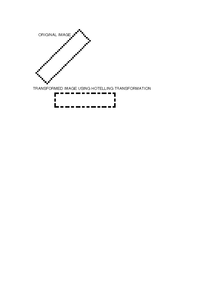
3. Numerical Linear Algebra
89
Figure 3-1. Hotelling transformation for binary image rotation
Note in the original Binary image, the Xpositions and Ypositions are
dependent to each other and hence the co-variance matrix is not the diagonal
matrix as mentioned below
CM=
102.2500 -80.9500
-80.9500 102.2500
But in the transformed Binary image, Xpositions and Ypositions are
independent to each other and hence the covariance matrix computed is the
diagonal matrix as given below
CT =
21.3000 0.0000
0.0000 183.2000
Note that the Diagonal values are Eigen values of the covariance
matrix C.
the Binary image created with ‘0’ (i.e.) Black. The image obtained is called
Transformed binary image using Hotelling transformation. Realize that the
Xposition and Yposition of Black pixels in the Transformed binary image
are independent to each other.

90 Chapter
3
Note that CM = TM’ * CT * TM
As the pixel positions of the image are represented as positive integers,
are transformed vectors are properly biased and rounded off.
1.3
Matlab Program
___________________________________________________________
hotellinggv.m
A=imread('Binimage','bmp');
A=double(A);
[x,y]=find(A==0);
vector=[x y];
Meanvector=sum(vector)/length(vector);
CM=(vector'*vector)/length(vector);
CM=CM-Meanvector'*Meanvector;
%Covariance matrix for the original set of vectors is CM
[E,V]=eig(C);
%Transformation Matrix
TM=E';
transvector=TM*(vector'-repmat(Meanvector',1,length(vector)));
xposition=fix(transvector(1,:)+abs(min(transvector(1,:)))+1);
yposition=fix(transvector(2,:)+abs(min(transvector(2,:)))+1);
B=zeros(50,50);
for i=1:1:length(xposition)
B(xposition(i),yposition(i))=1;
end
%Covariance matrix computed for transformed vectors is computed as CT
MeanvectorT=sum(transvector')/length(transvector');
CT=(transvector*transvector')/length(transvector');
CT=CT-MeanvectorT'*MeanvectorT;
figure
subplot(2,1,1)
imshow(A)
title('ORIGINAL IMAGE')
subplot(2,1,2)
imshow(uint8(B*255))
title('TRANSFORMED IMAGE USING HOTELLING TRANSFORMATION')
___________________________________________________________
3. Numerical Linear Algebra
91
2.
EIGEN BASIS
Group of vectors are described as the vector space. All the vectors in the
space are spanned by the particular set of orthonormal basis known as Eigen
basis as described below. (i.e) Any vector in the space is represented as the
linear combination of Eigen basis.
2.1
Example 1
The two dimensional vector are randomly generated and are plotted as given
below. The vectors mentioned in the diagram are the Eigen vectors. It is
computed as follows.
Figure 3-2. Vector space along with Eigen vectors
• Compute the co-variance matrix of the generated two
dimensional vectors
• Compute the Eigen values and the corresponding Eigen vectors.
• Direction of the Eigen vectors computed are parallel to the
vectors mentioned in the diagram. Note that they are orthonormal
to each other.
In the above described example, Eigen vectors are E
1
= [-0.2459 -0.9693]
and E
2
=[-0.9693 0.2459].
92 Chapter
3
Also, any vector in the generated vector space is represented as the linear
combination of E1 and E2. The co-efficients are obtained as the inner product
of vector and the corresponding Eigen vector.
For instance, the vector V
1
=[20 16] is represented as
C
1
E
1
+C
2
E
2
C
1
is obtained as the inner product of E
1
and V
1
C
2
is obtained as the inner product of E
2
and V
2
C
1
= -20.4269
C
2
= -15.4513
Thus V
1
= C
1
E
1
+C
2
E
2
= -20.4269 *[-0.2459 -0.9693]+ -15.4513 *[-0.9693 0.2459].
Eigen vectors corresponding to the insignificant Eigen values are
contributing less to the vector representation. In such situation number of
orthornormal Eigen basis to represent the particular vector is reduced.
Note that the vectors mentioned in the figure 3-3 is obtained by applying
KLT transformation to the vector space mentioned in the Fig 3-2. The Eigen
vectors for this space are E
1
=[1 0] and E
2
=[0 1]
Figure 3-3. Vector space after KLT and the corresponding eigen vectors

3. Numerical Linear Algebra
93
3.
SINGULAR VALUE DECOMPOSITION (SVD)
As discussed earlier any real square matrix ‘A’ can be diagonalized using
eigen matrix ‘E’ (every column vector is the eigen vector of the matrix ‘A’)
A=E D E
T
where ‘D’ is the diagonal matrix filled with Eigen values in the diagonal
Suppose if the matrix ‘A’ is the rectangular matrix of size mxn, then the
matrix ‘A’ can be represented as the follows
A=U ^ V
T
. This is called as Singular Value Decomposition.
AA
T
is the square matrix with size mxm. Using Eigen decomposition
AA
T
= U D
1
U
T
Similarly A
T
A of size nxn can be reprersented using Eigen
decomposition as
A
T
A= V D
2
V
T
If A = U ^ V
T
A
T
=V ^
T
U
T
Note that ^ and ^
T
are the same as the matrix is the diagonal matrix.
AA
T
= U ^ V
T
V ^
T
U
T
= U ^^
T
U
T
[Expected Result]
Similarly
A
T
A = V ^
T
U
T
U ^V
T
= V ^
T
^ V
T
[Expected Result]
The diagonal elements of the matrix ^ is obtained as the positive square
root of the diagonal elements of the matrix D
1
or D
2
. Note that the diagonal
elements of the matrix D
1
and D
2
are same except the addition or deletion of
zeros.
Thus the matrix A is represented as the product of the Eigen matrix
obtained from the matrix AA
T
, Eigen matrix obtained from the matrix A
T
A

94 Chapter
3
and the Diagonal matrix ^ obtained as the positive square root of the
elements of the eigen values computed for the matrix AA
T
(or) A
T
A
(i.e.) The Eigen values are same for both the matrices.
3.1
Example
The matrix A is applied to SVD as follows.
A =
1 2 3
4 5 6
U =
-0.3863 -0.9224
-0.9224
0.3863
V =
-0.4287 0.8060 0.4082
-0.5663 0.1124 -0.8165
-0.7039 -0.5812 0.4082
^ =
9.5080
0 0
0
0.7729
0
U*^*V' =
1.0000 2.0000 3.0000
4.0000 5.0000 6.0000
Eigen values of (A'*A) = E
1
-0.0000
0.5973
90.4027
Eigen values of (A*A’) = E
2
0.5973
90.4027
Note that the diagonal elements of the ^ is obtained as the square root of
E
1
or E
2
.
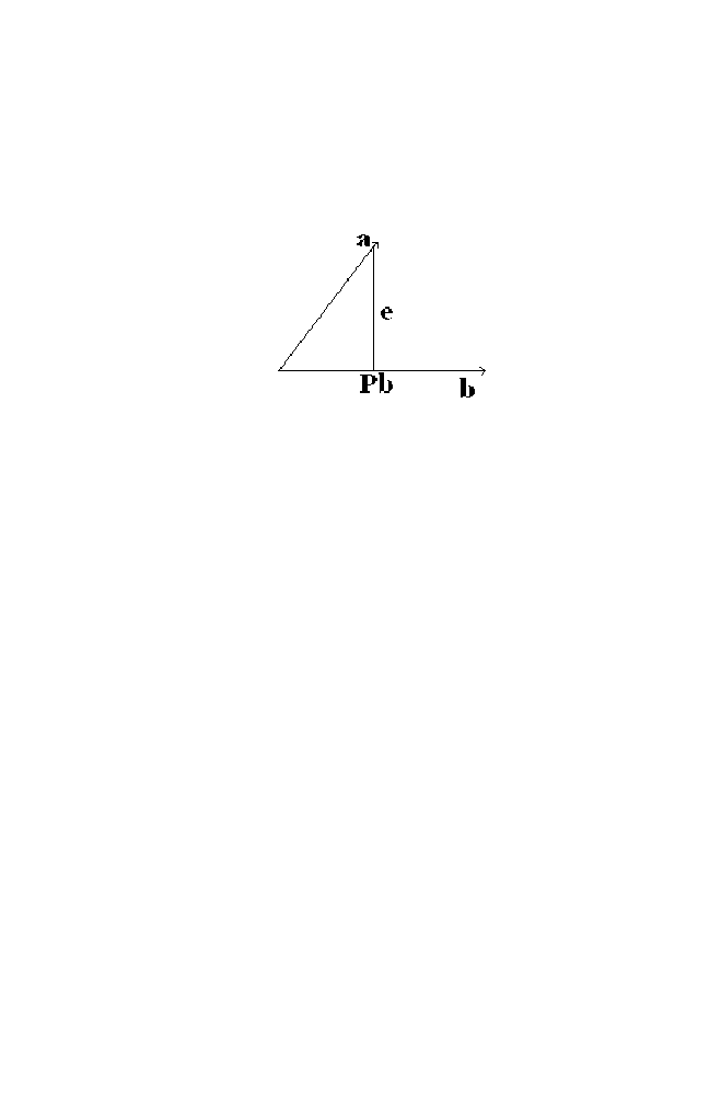
3. Numerical Linear Algebra
95
4.
PROJECTION MATRIX
4.1
Projection of the Vector ‘a’ on the Vector ‘b’
Figure 3-4. Projection Illustration
Consider two vectors a and b. The projection of the vector ‘a’ on ‘b’ is the
scaled version of the vector ‘b’ (i.e) Pb. The vector e is orthogonal to the
vector b as shown in the figure 3-3.
e=a-Pb
⇒ b
T
(a-Pb)
=0
⇒ b
T
a
=Pb
T
b
⇒P = (b
T
a) / (b
T
b)
Therefore the projection of the vector ‘a’ on ‘b’ is given as
bP = [b( b
T
a) ] /
[(b
T
b)].
The Projection matrix (In this case, ,it is the single element matrix) is
given as (bb
T
)/( b
T
b) = [P
M
]
Thus the projection of the vector ‘a’ on ‘b’ is given as [P
M
] a

96 Chapter
3
4.2
Projection of the Vector on the Plane Described
Figure 3-5. Projection of the vector on the plane
Consider the vector ‘a’ projected on the plane described by the vectors
‘x1’ and ‘x2’. Note that the matrix X =[x1 x2]. The vector ‘p’ can be
represented as the linear combination of the vector ‘x1’ and ‘x2’ (i.e)
column vectors of the matrix X as illustrated in the figure 3-4
p=u1*x1+u2*x2
p=[X] u1
u2
p=[X][s]
Also the error vector [a-p] is orthogonal to x1 and x2 as illustrated in the
figure.
⇒(a-Xs)
T
x1
=0 and (a-Xs)
T
x2
=0
Jointly represented as [a-Xs]
T
X
= 0
0
⇒a
T
X
=(Xs)
T
X
by Two Column Vectors of the Matrix ‘X’
The Linear combination of certain number of n-dimensional independent
vectors forms the vector space. Thus vector space is defined as the space
spanned by the set of independent vectors.

3. Numerical Linear Algebra
97
⇒X
T
a = X
T
(Xs)
⇒s=(X
T
X)
-1
X
T
a
Therefore the projected vector p=[X][s]=X(X
T
X)
-1
X
T
a
Thus projected matrix P
M
is defined as X(X
T
X)
-1
X
T
.Also the projected
vector p is represented as [P
M
] a
In general projection of the vector ‘a’ on the vector space spanned by the
column vectors of the matrix ‘A’ is given as A(A
T
A)
-1
A
T
a
4.2.1
Example
Consider the vector space spanned by the column vectors of the matrix
A= 1 3 7 6
4 6 2 4
1 7 6 4
The projection of the vector a= [1 2 3]
T
on the vector space spanned by the column vectors of the matrix A is
given using the formula A(A
T
A)
-1
A
T
a is given below
Projection matrix
P
M
= A(A
T
A)
-1
A
T
=
-0.2813 -0.5625 -0.6563
-0.1875 1.1250 0.0625
0.0313 0.1875 1.5313

98 Chapter
3
Projected vector is computed as A(A
T
A)
-1
A
T
a
= -3.3750
2.2500
5.0000
4.2.2
Example 2
The column vectors A, B and C are displayed below.
A=[10 2 6 5 9 8 5 0 8 4]
T
B= [6 8 9 7 2 4 9 9 4 9]
T
C=[43 26 44 29 32 34 35 24 35 32]
T
The column vector C is related to the column vectors A and B as the
linear combination as displayed below C = m*A+ n*B. The requirement is
to find the optimal value for the scaling constant m and n.
If C is in the space spanned by the column vectors of A and B, unique m
and n values can be computed easily. But if C is not in the space spanned by
the column vectors of A and B, the constants ‘m’ and ‘n’ are the best
estimated values such that C’=m*A+n*B is in the space spanned by the
column vectors A and B.
Also the mean squared error (i.e) E {(C-C’)
2
] is minimized. This is
obtained using projection matrix as described below.
The column vector C’ is the projection of the vector ‘C’ on the space
spanned by the vectors A and B.
Representing the vectors A and B in the matrix column wise to form the
matrix ‘P’.
Thus P= 10 6
2 8
6 9
5 7
9 2
8 4
5 9
0 9
8 4
4 9
3. Numerical Linear Algebra
99
The projection matrix is computed as PM=P*inv ((P*P
T
))*P
T
. Using the
projection matrix, the C’ column vector is obtained as the projection of the
column vector C as C’=PM*C.
C’= 44.3140
25.6450
39.9154
32.0289
31.4915
33.4768
36.9648
22.2118
33.4768
34.0142
Thus the best estimated values of the variable ‘m’ and ‘n’ are computed
as
10
6
-1
44.3140
2 8 25.6450
= 2.9506
2.4680
find the alternate values for the variables ‘m’ and ‘n’ which gives MSE less
than the 4.1678.
MSE is computed as E [(C-C’)
2
] = 4.1678. Note that it is not possible to
100 Chapter
3
5.
ORTHONORMAL VECTORS
The vectors a, b, c are defined as the orthogonal vectors if their inner product
matrix is the diagonal matrix. (i.e) dot product of the vector a with itself is
some constant, whereas the dot product of the vector a with b is 0.
If the diagonal matrix obtained is the identity matrix, then the vectors are
called as orthonormal vectors.
5.1
Gram-Schmidt Orthogonalization Procedure
Consider the set of independent vectors v1, v2 and v3 which spans the
particular vector space ‘S’. (i.e) All the vectors in the space ‘S’ are repre-
sented as the linear combination of the independent vectors (v2, v2, v3).
They are called basis.
It is possible to identify the another set of independent vectors o1, o2 and
o3 which spans the space S such that the vectors o1, o2 and o3 are
orthonormal to each other. The steps involved in obtaining the orthornormal
vectors corresponding to the independent vectors are described below.
Figure 3-6. Gram-Schmidt Orthogonalization procedure
Let ‘v1’ and ‘v2’ be the independent column vectors. The vector ‘v1’ is
treated as the reference vector. (i.e) Normalized ‘v1’ is treated as the one of
From the figure 3-5 p=v2- [(o1
T
v2) / (o1
T
o1)] o1. The orthonormal
vector is the normalized form of the vector ‘p’.
o2 = p / ||p||
Similarly the orthonormal vector ‘o3’ corresponding to the vector ‘v3’ is
obtained as follows.
the orthonormal vector ‘o1’= ‘v1/||v1||’. The orthogonal vector ‘p’ is
computed using the projection of the vector ‘v2’ on the vector ‘v1’.
3. Numerical Linear Algebra
101
q= v3- [(o1
T
v3) / (o1
T
o1)] o1] - [(o2
T
v3) / (o2
T
o2)] o2]
o3 =q / ||q||
5.2
Example
Consider the set of independent column vectors v1, v2 and v3 as displayed
below.
1 2 4
v1= 2 v2= 1 v3 = 2
3 4 3
The corresponding set of orthonormal vectors computed using Gram-
Schmidt orthogonalization procedure is given below.
0.2673 0.5203 0.8111
o1 = 0.5345 o2 = -0.7804 o3 = 0.3244
0.8018 0.3468 -0.4867
The dot product of the vectors o1, o2 and o3 is displayed in the matrix
form for illustration.
1.0000 -0.0000 0.0000
-0.0000 1.0000 0.0000
0.0000 0.0000 1.0000
Note that the matrix obtained is the identity matrix as expected.
5.3
Need for Orthonormal Basis
Suppose the vector ‘V’ in the vector space ‘S’ is represented as the linear
combination of the orthonormal basis computed in the section 5.1
9
V = 6
14
The co-efficients are obtained as the inner product of the vector ‘V’ and
the corresponding orthonormal basis.

102 Chapter
3
The co-efficients are
c1= V
T
*o1 = 16.8375
c2=V
T
*o2 = 4.8558
c3 =V
T
*o3 = 2.4333
Thus the vector V is represented as
V = c1*o1+c2*o2+c3*o3
Computing the co-efficients become easier if the basis are orthonormal to
each other and hence orthonormal basis is required.
If adding few more independent vectors increases the number of
independent vectors spanning the space, the space spanned by these vectors
also increases. The corresponding orthonormal vectors obtained using Gram-
Schmidt orthogonalization procedure shows that the orthonormal basis are
the same as that of the earlier except the inclusion of additional few
orthogonal basis corresponding to the additional independent vectors. Hence
the co-efficients of the already existing basis remains the same.
In the previous example if the vector chosen in the space spanned by the
vectors v1 and v2.
6
6 (say)
14
The vector can be represented as the linear combination of ‘o1’ and
‘o2’ with the corresponding co-efficients 16.0357 and 3.2950 respectively.
They are computed using inner product technique. Suppose the same vector
is represented as the linear combination of ‘o1’ ‘o2’ and ‘o3’, the
corresponding co-efficients are obtained as 16.0357, 3.2950 and 4.4409e-
015 respectively. Note that first two co-efficients remains unchanged and
also note that the value of the third co-efficient is almost insignificant for
representing the vector. This property is used in compression techniques in
which the significant co-efficients are stored rather than the vector itself.

3. Numerical Linear Algebra
103
5.4
M-file for Gram-Schmidt Orthogonalization
Procedure
gramgv.m
%Given the independent vectors as the input,Orthonormal vectors as the
%output computed using Gram-Schmidt Orthogonalization procedure
%Input vectors are arranged rowwise
function [res]=gramgv(x)
o{1}=x(1,:)/sqrt(sum(x(1,:).^2));
for k=2:1:size(x,1)
s=x(k,:);
for m=1:1:k-1
s=s - ((o{m}*x(k,:)')/(o{m}*o{m}'))*o{m} ;
end
o{k}=s/sqrt(sum(s.^2));
end
res=o;
6.
COMPUTATION OF THE POWERS
Consider the matrix A = 3 4 . The matrix A
100
is computed as
1 2
described below.
The matrix ‘A’ can be diagonalized using eigen matrix ‘E’ (every column
vector is the eigen vector of the matrix ‘A’) as described in the section 3
OF THE MATRIX ‘A’
104 Chapter
3
A=E D E
-1
Where ‘D’ is the diagonal matrix filled with Eigen values in the diagonal.
Consider the computation of the matrix A
2
=A A=EDE
-1
EDE
T
=EDDE
T
=ED
2
E
T
In general A
100
is using ED
100
E
T
For the given matrix ‘A’, eigen matrix ‘E’ is computed as
E= 0.9315 -0.8421 and the diagonal matrix D is given as follows
0.3637 0.5393
D = 4.5616
0
0
0.4384
Therefore A
100
is computed as ED
100
E
-1
=
5.06471.0e+065 7.90871.0e+065
1.97721.0e+065 3.08751.0e+065
Note that if all the eigen values in the Diagonal matrix described above is
less than 1, the matrix A
n
converges to the value zero when n tends to
infinity.
7.
DETERMINATION OF K
TH
ELEMENT
IN THE SEQUENCE
Let us consider the sequence 0, 1, 2, 3, 6, 11, 20, 37… in which fourth
element is the summation of three previous numbers. Fifth value is the
summation of 2, 3 and 4 value of the sequence and so on.
3. Numerical Linear Algebra
105
The problem is to obtain the value of the 100th element of the above
mentioned sequence. This is achieved using Eigen decomposition as
described below.
Let P
k
be the value of the k
th
position of the sequence.
P
k
= P
k-1
+ P
k-2 +
P
k-3
Let us define the matrix U
k
= P
k+2
P
k+1
P
k
P
k+3
U
k+1
= P
k+2
P
k+1
U
k+1
= 1 1 1 U
K
1 0 0
0 1 0
U
0
= 2
1
0
Let the matrix A be 1 1 1
1 0 1
0 1 0
Represent the vector U
0
as the linear combinations of Eigen vectors of
the matrix A.
The Eigen values and the corresponding Eigen vectors are computed and
displayed below.
Eigen values = [
λ
1
λ
2
λ
3
]
= [1.8393 -0.4196 + 0.6063i -0.4196 - 0.6063i]
Eigen vectors arranged in columnwise =[ E1 E2 E3] =
-0.8503 -0.1412 - 0.3752i -0.1412 + 0.3752i
-0.4623 -0.3094 + 0.4471i -0.3094 - 0.4471i
-0.2514 0.7374
0.7374
106 Chapter
3
Represent the matrix U
o
as the linear combinations of Eigen vectors.
2
1 =
0
-0.8503 -0.1412 - 0.3752i -0.1412 + 0.3752i c1
-0.4623 -0.3094 + 0.4471i -0.3094 - 0.4471i c2
-0.2514 0.7374
0.7374 c3
c1 -2.0649 + 0.0000i
c2 = -0.3520 + 0.1929i
c3 -0.3520 - 0.1929i
U
1
= A U
o
U
2
= A
2
U
o
…
U
k
= A
k
U
o
U
o
= c1*E1+c2*E2+c3*E3
AU
o
= c1*A*E1+c2*A*E2+c3*A*E3
= c1*
λ
1
*E1+c2*
λ
2
*E2+c3*
λ
3
*E3
Similarly
U
k
= A
k
U
o
= c1*
λ
1
k
*E1+c2*
λ
2
k
*E2+c3*
λ
3
k
*E3
Therefore U
100
is computed as
U
100
= 1.0e+026
5.1220 - 0.0000i
2.7848 - 0.0000i
1.5140 - 0.0000i
Therefore the 100th term in the sequence is given as 1.51401.0e+026
Let us compute 6
th
term using the method given above
3. Numerical Linear Algebra
107
U
6
=68.0000 - 0.0000i
37.0000 - 0.0000i
20.0000 - 0.0000i
Therefore 6
th
term is 20 as expected (see the sequence).
8.
COMPUTATION OF EXPONENTIAL
Let A be the matrix, which can be diagonalizable using Eigen matrix as
A=EDE
-1
. e
A
can be computed using series expansion as given below.
e
A
= I + A +(A
2
)/2! +(A
3
)/3!+…..
= I +EDE
-1
+(EDE
-1
EDE
-1
) /2! +(EDE
-1
EDE
-1
EDE
-1
)/3!+…
= ED
0
E
-1
+EDE
-1
+ (ED
2
E
-1
)/2! +(ED
3
E
-1
)/3! +…
= E[D
0
+ (D/1! )+(D
2
/2!) + (D
3
/3!)
+(D
4
/4!)
+…] E
-1
= E e
D
E
-1
8.1
Example
A = 1 1 = EDE
-1
1 0
0.5257 -0.8507 -0.6180 0 0.5257 -0.8507
-0.8507 -0.5257 0 1.6180 -0.8507 -0.5257
Therefore e
A
is computed as
E e
D
E
-1
=
0.5257 -0.8507 e
-0.6180
0.5257 -0.8507
-0.8507 -0.5257 0 e
1.6180
-0.8507 -0.5257
= 3.7982 2.0143
2.0143 1.7839
0
OF THE MATRIX
108 Chapter
3
9.
SOLVING DIFFERENTIAL EQUATION USING
EIGEN DECOMPOSITION
Consider the problem of solving the third order differential equation as
given below.
∂
3
u /
∂t
3
+2
∂
2
u /
∂t
2
-
∂u / ∂t +u = 0 with the initial condition given
U’’(0)=3, U’(0)=1, U(0)= -1.
Representing the above equation in the form of matrix representation.
V = U’’
U’
U
V’ = U’’’
U’’
U’
V’= -2 1 1 V
1 0
0
0 1 0
V = c1 e
λ1 t
E
1
+c2 e
λ2 t
E
2
+ c3 e
λ3 t
E
3
Where c1, c2 and c3 are the constants obtained using initial conditions.
E1, E2 and E3 are the eigen vectors of the matrix A corresponding to the
eigen values
λ
1
,
λ
2,
λ
3
respectively.
The Eigen vectors and the eigen values of the matrix A are displayed
below.
λ
1
= -2.2470
λ
2
=
0.8019
λ
3
= -0.5550
E1= [-0.8990 0.4001 -0.1781]
T

3. Numerical Linear Algebra
109
E2= [-0.4484 -0.5592 -0.6973]
T
E3= [0.2600 -0.4686 0.8443]
T
Thus V= U’’
U’ is obtained as follows
U
U’’= c1 e
-2.2470 t
(-0.8990) + c2 e
0.8019
t
(-0.4484) + c3 e
-0.5550 t
(0.2600)
U’= c1 e
-2.2470 t
(0.4001) + c2 e
0.8019
t
(-0.5592) + c3 e
-0.5550 t
(-0.4686)
U= c1 e
-2.2470 t
(-0.1781) + c2 e
0.8019
t
(-0.6973) + c3 e
-0.5550 t
(0.8443)
The values of the constants can be solved using the initial conditions
using the set of equations given below.
U’’(0) =3 =(-0.8990) c1 + (-0.4484) c2
+ (0.2600) c3
U’(0) =1 = (0.4001) c1 + (-0.5592) c2
+ (-0.4686) c3
U(0) = -1 = (-0.1781)c1 +
(-0.6973)c2
+ (0.8443) c3
Thus c1= -3.4815, c2= -1.5790, c3= -3.2227
10.
COMPUTATION OF PSEUDO INVERSE
Let us consider the matrix A = 2 3 4
3 4 5
Decompose the matrix ‘A’ using Singular Value Decomposition.
OF THE MATRIX
110 Chapter
3
A= [P ][ Q ][ R
T
]
A= -0.6057 -0.7957 8.8839 0 0
-0.7957 0.6057 0 0.2757 0
-0.4051 -0.5628 -0.7205
0.8181 0.1288 -0.5605
0.4082 -0.8165 0.4082
Pseudo inverse matrix A
+
is given as
A
+
= {[R] [Q+][P
T
]}
[Q
+
] = 1/ 8.8839
0
0
1/ 0.2757
0
0
= 0.1126
0
0 3.6268
0
0
QQ
+
= 1 0
0 1
A
+
= -2.3333 1.8333
-0.3333 0.3333
1.6667 -1.6667
AA
+
= 1 0
0 1

3. Numerical Linear Algebra
111
11.
COMPUTATION OF TRANSFORMATION
MATRICES
If the vectors in the space1 are spanned by the independent vectors u1, u2,
u3, … un. Also if the vectors in the space2 are spanned by the independent
vectors v1, v2 …vn . They are called basis of the respective spaces.
Suppose the vector ‘u’ in the space 1 is mapped to the vector v in the
space 2.
(i.e.) T (u) = v. The vector ‘v’ can be represented as the linear
combinations of the independent vectors v1, v2, …vn.
Similarly the transformation of the basis vector u1 in the space1 can be
represented as the linear combinations of v1, v2, v3…vn.
Therefore T (u1) =a
11
v1+ a
12
v2+ a
13
v3+ a
14
v4 + … a
1n
vn
Similarly T (u2) =a
21
v1+ a
22
v2+ a
23
v3+ a
24
v4 + … a
2n
vn
…
T (un) =an
1
v1+ a
n2
v2+ a
n3
v3+ a
n4
v4 + … a
nn
vn
The co-efficients of the vector v1, v2, v3 .. vn in the above mentioned
equation are arranged in the vector form and are called co-efficient vector as
given below.
The vector [a
11
a
12
a
13
a
14 …
a
1n
] is the co-efficient vector associated with
the vector T(u1) which is in the space 2. Similarly the vector
[a
21
a
22
a
23
a
24 …
a
2n
] is the co-efficient vector associated with the vector
T(u2).
Consider the vector u1 in the space 1 which can also be represented as
the linear combinations of the basis vectors u1, u2, u3, …un as given below.
u1=1*u1+0*u2+0*u3+….0*un.
In this case [1 0 0 0 …0] is the co-efficient vector associated with the
vector u1 in the space1.

112 Chapter
3
As mentioned earlier the any vector ‘u’ in the space 1 and the
corresponding mapped vector v in the space 2 can also have their associated
coefficient vectors. Let [p1, p2, p3, …pn] be the co-efficient vector associated
with the vector ‘u’ and [q1, q2, q3…qn] be the co-efficient vector associated
with the vector ‘v’.
The matrix relating the co-efficient vector of the particular vector in the
space 1 and the co-efficient vector of the corresponding mapped vector in
the space 2 is called transformation matrix and is computed as described
below.
(i.e.)
[p1 p2 p3 p4 …pn]
T
[TM] = [q1 q2 q3 q4 … qn]
T
The transformation matrix is obtained using the co-efficient vectors
computed for the T(u1), T(u2),…T(un) in the space 2 where u1,u2 u3,..un
are the independent vectors which spans the space 1.
Thus TM = a11 a21 a31 a41 a51 …an1
a12 a22 a32 a42 a52 …an2
a13 a23 a33 a43 a53 …an3
a14 a24 a34 a44 a54 …an4
…
a1n a2n a3n a4n a5n …ann
For example the vector u1 with co-efficient vector [1 0 0 0 0 0 0…0] is
mapped to the vector T(u1) whose co-efficient vector is obtained using TM
as
a11 a21 a31 a41 a51 …an1 1 a11
a12 a22 a32 a42 a52 …an2 0 a12
a13 a23 a33 a43 a53 …an3 0 = a13
a14 a24 a34 a44 a54 …an4 0 a14
…
a1n a2n a3n a4n a5n …ann 0 a1n
The co-efficient vector obtained is as expected.

3. Numerical Linear Algebra
113
11.1
Computation of Transformation Matrix
Consider that the vector space 1 is spanned by the 4 basis as given below.
1 0 0 0
v1= 0 v2= 1 v3= 0 v4= 0
0 0 1 0
0 0 0 1
Every vector in the space spanned by the basis vector given above is
mapped to the vector in vector space 2 called as Fourier space. Fourier
transformation of the basis vectors v1, v2, v3, v4 are given as
T(v1) = [1 1 1 1 ]
T
T(v2) = [1.0000 0 - 1.0000i -1.0000 0 + 1.0000i ]
T
T(v3) = [1 -1 1 -1]
T
T(v4) = [1.0000 0 + 1.0000i -1.0000 0 - 1.0000i ]
T
The basis vectors of the Fourier space is given as
f1 = (1/2)* [1 1 1 1 ]
T
f2 = (1/2) * [1.0000 0 - 1.0000i -1.0000 0 + 1.0000i ]
T
f3 = (1/2) * [1 -1 1 -1]
T
f4 = (1/2)* [1.0000 0 + 1.0000i -1.0000 0 - 1.0000i ]
T
The transformed vector T(v1) is represented as the linear combination of
f1, f2, f3, f4. Note that the basis are orthonormal basis
for the Fourier Transformation

114 Chapter
3
The co-efficient vector is obtained as the inner product of the vector
T(v1) with the corresponding basis.
[T(v1)]
T
f1
*
= [2] [Note that the inner product complex numbers ‘a’
and ‘b’ is computed as a
T
b*]
[T(v1)]
T
f2
*
= [0]
[T(v1)]
T
f1
*
= [ 0]
[T(v1)]
T
f1
*
= [0]
Therefore the co-efficient vector associated with the vector T(v1) is
given as [2 0 0 0]
T
Similarly the co-efficient vector associated with the vector T(v2), T(v3)
and T(v4) is given as [0 2 0 0]
T
, [0 0 2 0]
T
and [0 0 0 2]
T
respectively.
Thus the transformation matrix for the Fourier transform is given as
2 0 0 0
0 2 0 0
0 0 2 0
0 0 0 2
As the transformation matrix is the diagonal matrix with ‘2’ as the
diagonal elements, the co-efficient vector for any vector in the Vector space
1 is ‘coef ’ then the co-efficient vector for the corresponding mapped vector
in the Vector space 2 (Fourier domain) is given be 2*c.
Thus the Fourier transformation of the vector [2 3 4 1] is given as the
1 1 1 1 2 * 2 10
1 -i -1 i 3 * 2 -2-i
(1/2) 1 -1 1 -1 4 * 2 = 2
1 i -1 -i 1 * 2 -2+2i
In the same fashion, DCT, DST the transformation matrix is the diagonal
matrix and hence the transformation values can be easily obtained using
simple matrix multiplication as described above.

3. Numerical Linear Algebra
115
11.2
Basis Co-efficient Transformation
Consider the 4-dimensional vector space which are spanned by the basis
u1=[1 0 0 0]
T
, u2=[0 1 0 0]
T
and u3=[0 0 1 0]
T
and u4=[0 0 0 1]
T
. Consider
another set of orthonormal basis which spans the space.
v1 = (1/2)* [1 1 1 1 ]
T
v2 = (1/2) * [1.0000 0 - 1.0000i -1.0000 0 + 1.0000i ]
T
v3 = (1/2) * [1 -1 1 -1]
T
v4 = (1/2)* [1.0000 0 + 1.0000i -1.0000 0 - 1.0000i ]
T
Any vector in the space can be represented as the linear combination of
u1, u2, u3 and u4. The same vector in the space can be represented as the
linear combination of v1, v2, v3 and v4.
Consider the transformation T which transforms the vector v is
represented as T(v) and is equal to v.
v is represented as the linear combination of u1 u2 u3 and u4.Let the co-
efficient vector be [p1 p2 p3 p4]
T(v)=v is represented as the linear combination of v1,v2,v3,v4.Let the
co-efficient vector be [q1 q2 q3 q4].
The transformation matrix which converts the co-efficient vector
[p1 p2 p3 p4] into the co-efficient vector [q1 q2 q3 q4] is transformation
matrix for the change of basis. It is obtained as described below.
T([1 0 0 0])=[1 0 0 0] is represented as 0.5*v1+0.5*v2+0.5*v3+0.5*v4
T([0 1 0 0])=[0 1 0 0] is represented as
0.5*v1 + ( 0.5 i )*v2+ (-0.5)*v3+ (-0.5 i)*v4
T([0 0 1 0])=[0 0 1 0] is represented as
0.5*v1 + (- 0.5)*v2+ (0.5)*v3+ (- 0.5 ) *v4
T([0 0 0 1])=[0 0 0 1] is represented as
0.5*v1 + (- 0.5 i)*v2+ (- 0.5)*v3+ ( 0.5 i) *v4
116 Chapter
3
There the transformation matrix which converts the co-efficients of the
particular basis into the co-efficients of the another set of basis belongs to
the same space is given as
0.5 0.5 0.5 0.5
0.5 0.5i -0.5 -0.5i
0.5 -0.5 0.5 -0.5
0.5 -0.5i -0.5 0.5i
For instant consider the vector [2 3 4 5] can be represented using the
basis u1, u2, u3, u4 with co-efficients [2 3 4 5]. The vector [2 3 4 5] can be
represented using the basis v1, v2, v3, v4 using the co-efficients computed
as
0.5 0.5 0.5 0.5 2 7
0.5 0.5i -0.5 -0.5i 3 = -1-i
0.5 -0.5 0.5 -0.5 4 -1
0.5 -0.5i -0.5 0.5i 5 -1+i
(i.e.) 7*(v1)+(-1-I)*v2+(-1)*v3+(-1+i)*v4 = [2 3 4 5]
Thus the transformation matrix which converts the co-efficients of the
particular vector represented using the basis ‘u’ into the co-efficients of the
same vector represented using the basis ‘v’.
If there are only few significant co-efficients obtained when represented
using the particular set of basis, data compression is achieved. (See chapter
4). This property is called data compaction property of the transformation.
Discrete Cosine Transformation (DCT) is having very high data compaction
property. Hence JPEG (Joint Photographic expert group) is using DCT for
image compression. Also JPEG2000 standard is using DWT (Discrete
Wavelet Transformation) for image compression.

3. Numerical Linear Algebra
117
11.3
Transformation Matrix for
Consider the group of two dimensional vectors collected randomly forms the
vector space. This is consider as the subspace spanned by the independent
basis E1=[-0.2459 -0.9693]
T
and E
2
=[-0.9693 0.2459]
T
(see section 2-1).
The vector [1 0] is represented as the linear combination u1 and u2 as [1
0] = 1*u1+0*u2.The transformed vector of [1 0] is the same vectors itself
(i.e.)[1 0].The vector [1 0] is represented as the linear combinations of Eigen
[0 1] is represented as the linear combination of u1 and u2 as [0 1]
T
=
0*u1+1*u2 and its transformed vector [0 1] is represented as the linear
combination of E1 and E2 as given by -0.9693*E1 +0.2459*E2.
Thus the transformation matrix which converts the co-efficients of the
basis u1 and u2 into the co-efficients of the Eigen basis E1 and E2 for the
particular vector in the space.
TM = -0.2459 -0.9693
-0.9693 -0.2459
Note that the transformation matrix consists of Eigen basis arranged
row wise.
11.4
Transformation Matrix for
Consider the 8-dimensional space spanned by the 8 independent vectors
u1= [1 0 0 0 0 0 0 0]
T
u2= [0 1 0 0 0 0 0 0]
T
u3= [0 0 1 0 0 0 0 0]
T
u4= [0 0 0 1 0 0 0 0]
T
u5= [0 0 0 0 1 0 0 0]
T
u6= [0 0 0 0 0 1 0 0]
T
u7= [0 0 0 0 0 0 1 0]
T
u8= [0 0 0 0 0 0 0 1]
T
Obtaining Co-efficient
of Eigen Basis
Obtaining Co-efficient
of Wavelet Basis
vectors u1 = [1 0 ]
T
and u2=[0 1]
T
. The subspace is spanned by the Eigen
basis given by -0.2459*E1+(-0.9693)*E2 =[ 1 0 ]. Similarly the vector

118 Chapter
3
Consider any vector in the space can also be represented as the linear
combination of Wavelet basis as described below. Note that orthonormal
basis
w1= (1/sqrt(8)) [1 1 1 1 1 1 1 1]
T
w2= (1/sqrt(8)) [1 1 1 1 -1 -1 -1 -1]
T
w3= (1/sqrt(4)) [1 1 -1 -1 0 0 0 0]
T
w4= (1/sqrt(4)) [0 0 0 0 1 1 -1 -1]
T
w5= (1/sqrt(2)) [1 -1 0 0 0 0 0 0]
T
w6= (1/sqrt(2)) [0 0 1 -1 0 0 0 0]
T
w7= (1/sqrt(2)) [0 0 0 0 1 -1 0 0]
T
w8= (1/sqrt(2)) [0 0 0 0 0 0 1 -1]
T
As described in the section 11.3 the transformation matrix which
converts the co-efficient of the basis u1,u2,…u8 into the co-efficient of the
basis w1, w2, w3,…w8 for the particular vector is computed and is displayed
below.
0.3536 0.3536
0.3536
0.3536 0.3536 0.3536
0.3536
0.3536
0.3536 0.3536
0.3536
0.3536 -0.3536 -0.3536 -0.3536 -0.3536
0.5000 0.5000 -0.5000
-0.5000 0
0
0
0
0
0
0
0
0.5000
0.5000 -0.5000
-0.5000
0.7071 - 0.7071 0
0
0
0
0
0
0
0
0.7071
0.7071
0
0
0
0
0
0
0
0
0.7071
0.7071
0
0
0
0
0
0
0
0
0.7071
0.7071
Note that the transformation matrix consists of the wavelet basis arranged
row wise.
12.
SYSTEM STABILITY TEST USING
EIGEN VALUES
Input signal and output signal of the system are usually related with
differential equation. The output signal is solved using the eigen
decomposition as described in the section 9. The general expression of the
output signal is of the form output (t)=c1 e
λ1 t
E
1
+c2 e
λ2 t
E
2
+ c3 e
λ3 t
E
3.
where
λ1, λ2 and λ3 are the eigen values. E
1
, E2 and E3 are the eigen
vectors of the matrix described in the section 9.
3. Numerical Linear Algebra
119
From the above equation it is observed that Output (t) is bounded only
when all the eigen values are less than 0 (i.e.) negative values. This is the test
for stability of the system using eigen values.
13.
POSITIVE DEFINITE MATRIX TEST FOR
MINIMA LOCATION OF THE FUNCTION
F (X1, X2, X3, … XN)
Represent the equation as the product of three matrices
[x
1
x
2
x
3
] 2 -1 0
x
1
-1 2 -1
x
2
0 -1 2
x
3
If the matrix 2 -1 0 is the positive definite matrix, then the
-1 2 -1
0 -1 2
function f(x) = 2 x
1
2
+ 2 x
2
2
+2 x
3
2
-2 x
1
x
2
-2 x
2
x
3
is the minima function
and the minima occurs at the point where the slope is zero (i.e.) first
derivative is zero. If all the eigen values of the matrix are positive, then the
matrix is positive definite matrix. Thus sign of all the eigen values of the
14.
WAVELET TRANSFORMATION USING
The 1D signal can be analyzed by using wavelet transformation. This can be
used to compress the data and to denoise the signal. Wavelet transformation
of the 1D signal contains the information regarding the low frequency
content of the signal, which is called approximation co-efficients and the
Consider the function 2 x
1
2
+ 2 x
2
2
+2 x
3
2
-2 x
1
x
2
-2 x
2
x
3
. To find the
minima of the function f(x), partial differentiate the function with respect to
x1, x2, x3 and equate to zero and solve for x1, x2, x3 to get (x
0
, y
0
, z
0
). The
slope at this point (x
0
, y
0
, z
0
) is zero. To confirm that the points so obtained
are minima, all the partial second derivative values are positive. This is
tested using matrix technique as described below.
matrix defined above decides whether the point (x
0
, y
0
, z
0
) at which the slope
is zero is minima or not.
MATRIX METHOD

120 Chapter
3
information regarding high frequency content of the signal, which is called
detail co-efficients. The wavelet transformation of the signal using matrix
method is described below.
14.1
Haar Transformation
Consider the signal with number of samples N. Form the Haar matrix with
size NXN and with the diagonal matrices filled up with the matrix given
below.
½ ½
½ - ½
For N=8, the matrix obtained is
½ ½ 0 0 0 0 0 0
½ - ½ 0 0 0 0 0 0
0 0 ½ ½ 0 0 0 0
TM1 0 0 ½ -½ 0 0 0 0
0 0 0 0 ½ ½ 0 0
0 0 0 0 ½ - ½ 0 0
0 0 0 0 0 0 ½ ½
0 0 0 0 0 0 ½ -½
Multiply the matrix TM1 with the is the signal data [d0 d1 d2 d3 d4 d5d6
d7 ] to obtain first level decomposition of Haar transformation.
I level Haar decomposition of the signal
[½ (d0+d1) ½ (d2-d3) ½ (d4+d5) ½ (d6-d7) ]
The samples ½ (d0+d1) ½ (d4+d5) are the average samples. They are
called approximated co-efficients of the signal at the first level. The samples
½ (d2-d3) ½ (d6-d7) are called detail co-efficients of the signal at the first
level.
Thus Approximation 1 = [½ (d0+d1) ½(d4+d5)]
Detail 1= [½ (d2-d3) ½(d6-d7) ]

3. Numerical Linear Algebra
121
The approximated co-efficients of the signal obtained in the first level
(Approximation 1) is further decomposed using Haar transformation to
obtain approximation and detail co-efficients of the second level using the
transformation matrix as given below.
½ ½ 0 0
TM2 = ½ -½ 0 0
0 0 ½ ½
0 0 ½ -½
Multiply the matrix [TM2] with the approximated data obtained in the
first level decomposition to obtain approximation and detail co-efficient of
the signal at the second level.
Thus second level approximation is given as
Approximation 2 = [½ ( ½ (d0+d1) + ½ (d4+d5) )]
= ¼ [ d0+d1+d4+d5]
Detail 2 = [½ ( ½ (d0+d1) - ½ (d4+d5) )]
= ¼ [d0 + d 1 - d4 - d5]
Note that approximation co-efficient in the first level and second level
are the low frequency information derived from the signal. Similarly the
detail co-efficient in the first level and the second level are the high
frequency information derived from the signal.
The Approximation 2, Detail 1 and Detail 2 completely describes the
signal. It is possible to reconstruct the signal using Approximation 2, Detail2
and Detail 2 co-efficients of the signal.
Reconstruction of the signal is obtained using the inverse Haar matrix
Formed with the diagonal matrices filled up with the matrix
1 1
1 -1

122 Chapter
3
For instance steps involved in reconstructing the signal for N=8 is given
below.
• Form the vector with the elements filled up with approximation 2 and
detail 2
[¼ [ d0+d1+d4+d5] ¼ [d0 + d 1 - d4 - d5] ]
• Form the Inverse transformation matrix 1
1 -1 0 0
1 -1 0 0
[ITM1] = 0 0 1 1
0 0 1 -1
• Multiply the vector with the matrix to obtain Approximation 1 and detail
1 in the jumbled order as [½ (d0+d1) ½ (d2-d3) ½ (d4+d5) ½(d6-d7) ]
• Form the inverse transformation matrix ITM2
[ITM2] = 1 1 0 0 0 0 0 0
1 -1 0 0 0 0 0 0
0 0 1 1 0 0 0 0
0 0 1 -1 0 0 0 0
0 0 0 0 1 1 0 0
0 0 0 0 1 -1 0 0
0 0 0 0 0 0 1 1
0 0 0 0 0 0 1 -1
• Multiply the vector obtained in jumbled order as mentioned above with
the matrix [ITM2] to obtain the original signal [d0 d1 d2 d3 d4 d5 d6 d7]
14.1.1
Example
Consider the signal x(n) =a=sin(2*pi*n)+sin(2*pi*100*n) with number
of samples =512 and sampling frequency Fs =512. The Haar
transformation is applied to the signal. The approximation and detail co-
efficients are obtained as described above and is displayed below for
illustration. Note that approximation co-efficients is the low frequency
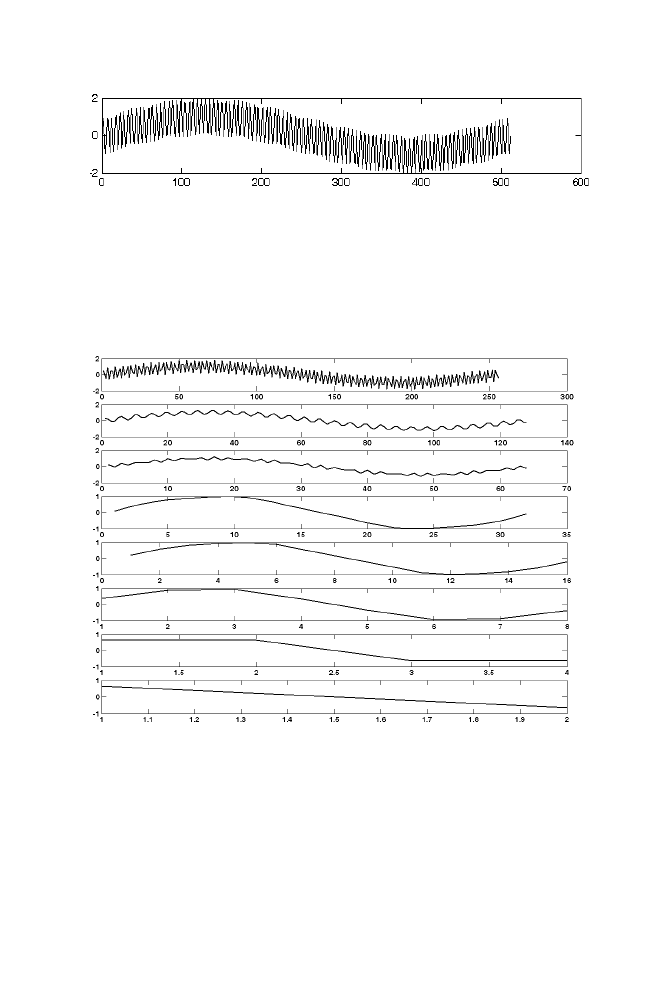
3. Numerical Linear Algebra
123
Figure 3-7. Original signal used for Haar decomposition
Figure 3-8. Approximation co-efficients obtained using Haar transformation
information derived from the signal and detail co-efficients is the high
frequency information derived form the signal.
The signal is reconstructed back using inverse Haar transformation and
the original signal along with reconstructed signal is displayed below.
124 Chapter
3
Figure 3-9. Detail co-efficients obtained using Haar transformation
Figure 3-10. Illustration of Inverse Haar Transformation

3. Numerical Linear Algebra
125
14.1.2
M-file for haar forward and inverse transformation
___________________________________________________________
haartrans.m
i=0:1/511:1;
a=sin(2*pi*i)+sin(2*pi*100*i);
plot(a)
figure
s=length(i);
for i=1:1:log2(s)
temp=createhaarmatrix(length(a))*a';
temp=reshape(temp,2,length(temp)/2);
approx{i}=temp(1,:);
det{i}=temp(2,:);
a=approx{i};
end
for k=1:1:(length(approx)-1)
subplot((length(approx)-1),1,k)
plot(approx{k})
title(strcat('approx',num2str(k)))
end
subplot(
figure
for k=1:1:(length(approx)-1)
subplot((length(approx)-1),1,k)
plot(det{k})
title(strcat('detail',num2str(k)))
end
___________________________________________________________
createhaarmatrix.m
function [res]=createhaarmatrix(m)
temp1=[ones(1,m/2);(-1)*ones(1,m/2)];
temp1=reshape(temp1,1,size(temp1,1)*size(temp1,2));
d1=temp1.*(1/2);
temp2=[ones(1,m/2);zeros(1,m/2)];
temp2=reshape(temp2,1,size(temp2,1)*size(temp2,2));
d2=(1/2)*temp2(1:1:length(temp2)-1);
res=diag(d1)+diag(d2,1)+diag(d2,-1);

126 Chapter
3
haarinvtrans.m
app=approx{8};
for i=(log2(s)-1):-1:1
a=[app;det{i}];
a=reshape(a,1,size(a,1)*size(a,2));
app=createinvhaarmatrix(length(a))*a';
app=app';
end
figure
subplot(2,1,1)
i=0:1/511:1;
a=sin(2*pi*i)+sin(2*pi*100*i);
plot(a)
title('Original signal');
subplot(2,1,2)
plot(app)
title('Reconstructed signal');
__________________________________________________________
createinvhaarmatrix.m
function [res]=createinvhaarmatrix(m)
temp1=[ones(1,m/2);(-1)*ones(1,m/2)];
temp1=reshape(temp1,1,size(temp1,1)*size(temp1,2));
d1=temp1;
temp2=[ones(1,m/2);zeros(1,m/2)];
temp2=reshape(temp2,1,size(temp2,1)*size(temp2,2));
d2=temp2(1:1:length(temp2)-1);
res=diag(d1)+diag(d2,1)+diag(d2,-1);
3. Numerical Linear Algebra
127
14.2
Daubechies- 4 Transformation
Consider the signal consists of N samples. Form the Daubechies
Transformation Matrix [DTM 1] with diagonal matrices filled up with the
matrix ‘D’ given below.
[(1+
√3) / 4√2] [(3+√3) / 4√2] [(3-√3) / 4√2] [(1-√3) / 4√2]
[(1-
√3) / 4√2] - [(3-√3) / 4√2] [(3+√3) / 4√2] -(1+√3) / 4√2]
For simplicity matrix D is represented as follows.
a0 a1 a2 a3
D =
b0 b1 b2 b3
For N=8, the matrix ‘DTM1’ is formed as given below.
a0
a1
a2
a3
0
0
0
0
0
0
b0
b1
b2
b3
0
0
0
0
0
0
0 0 a0
a1
a2
a3
0 0 0 0
0 0 b0
b1
b2
b3
0 0 0 0
0 0 0 0 a0
a1
a2
a3
0 0
0 0 0 0 b0
b1
b2
b3
0 0
0
0 0
0
0
0
a0
a1
a2
a3
0
0 0
0
0
0
b0
b1
b2
b3
Note that the matrix ‘D’ are arranged with overlapping in the diagonal of
the matrix ‘DTM 1’. Compare with the Haar transformation in which the
matrix are arranged without overlapping. Also note that the size of the
matrix is of size 8X10 for the signal of size 1x8. So 1x8 sized signal is
extended to the size 1x10 with 9
th
and 10
th
samples are filled up with 1
st
and
2
nd
samples respectively. [Assuming that the signals are repeated cyclically].
The steps involved in obtaining the approximation and detail co-
efficients are as described in the section 14.1 for Haar transformation.

128 Chapter
3
Similarly to reconstruct the signal, inverse Daubechies matrix is formed
with the diagonal matrices filled up with the matrix [ID] as given below.
[ID] = a3 b3 a1 b1
a4 b4 a2 b2
For N=8 the second level Inverse Daubechies matrix DITM2 is given as
a3 b3 a1 b1 0 0 0 0 0 0
a4 b4 a2 b2 0 0 0 0 0 0
0 0 a3 b3 a1
b1 0 0 0 0
0 0 a4 b4 a2
b2 0 0 0 0
0 0 0 0 a3
b3 a1 B1 0 0
0 0 0 0 a4
b4 a2 B2 0 0
0 0 0 0 0 0 a3 B3 a1 b1
0 0 0 0 0 0 a4 B4 a2 b2
Similar to the DTM 1,size of the matrix is 8x10. Also similar to forward
transformation, 1x8 sized wavelet co-efficients obtained in the forward
transformation is extended to 1x10-sized co-efficients with 1st and 2
nd
co-
efficients filled up with the last two co-efficients of the wavelet co-efficients.
The steps involved in reconstructing the signal are same as that of the
Haar transformation except that in Daubechies matrix the diagonal matrices
are arranged with overlapping whereas in Haar matrix there is no
overlapping.
14.2.1
Example
Consider the signal x(n) =a=sin (2*pi*n)+sin(2*pi*100*n) with number of
samples = 128 and sampling frequency Fs = 128. The Daubechies
transformation is applied to the signal The approximation and detail co-
efficients are obtained as described above and is displayed below for
illustration. Note that approximation co-efficients is the low frequency
information derived from the signal and detail co-efficients is the high
frequency information derived from the signal.
3. Numerical Linear Algebra
129
Figure 3-11. Original signal used for Daubechies 4 wavelet decomposition
Figure
3
-
12
. Approximation co-efficients at different levels
130 Chapter
3
Figure 3-13 Detail Co-efficients at different levels
Figure 3-14 Illustration of Inverse Daubechies 4 transformation

3. Numerical Linear Algebra
131
14.2.2
M-file for daubechies 4 forward and inverse transformation
___________________________________________________________
daub4trans.m
i=0:1/127:1;
a=sin(2*pi*i)+sin(2*pi*100*i);
plot(a)
figure
s=length(a);
for i=1:1:log2(s) -2
a=[a a(1:2)];
i
temp=createdaubmatrix(length(a)-2)*a';
temp=temp(1:1:length(temp));
temp=reshape(temp,2,length(temp)/2);
approx{i}=temp(1,:);
det{i}=temp(2,:);
a=approx{i};
end
for k=1:1:(length(approx)-1)
subplot((length(approx)-1),1,k)
plot(approx{k})
title(strcat('approx',num2str(k)))
end
figure
for k=1:1:(length(approx)-1)
subplot((length(approx)-1),1,k)
plot(det{k})
title(strcat('detail',num2str(k)))
end

132 Chapter
3
______________________________________________________________________
createdaubmatrix.m
function [res]=createdaubmatrix(m)
a=[(1+sqrt(3))/(4*sqrt(2))
(3+sqrt(3))/(4*sqrt(2))
(3-sqrt(3))/(4*sqrt(2))
(1-sqrt(3))/(4*sqrt(2))];
b=[(1-sqrt(3))/(4*sqrt(2))
-(3-sqrt(3))/(4*sqrt(2))
(3+sqrt(3))/(4*sqrt(2))
-(1+sqrt(3))/(4*sqrt(2))];
t1=repmat([a(2) b(3)],1,(m/2));
t2=repmat([a(3) b(4)],1,m/2);
t3=repmat([a(4) 0],1,m/2);
t4=repmat([b(1) 0],1,m/2);
res=diag(repmat([a(1) b(2)],1,m/2)) + diag(t1(1:1:m-1),1)
+diag(t2(1:1:m-2),2)+diag(t3(1:1:m-3),3)+diag(t4(1:1:m-1),-1) ;
res=[res [zeros(1,m-2) res(1,3) res(2,3)]' [zeros(1,m-2) res(1,4) res(2,4)]'];
______________________________________________________________________
daub4invtrans.m
app=approx{log2(s)-2};
for i=(log2(s)-2):-1:1
a=[app;det{i}];
a=reshape(a,1,size(a,1)*size(a,2));
a=[ a(length(a)-1:1:length(a)) a];
app=createdaubinvmatrix(length(a)-2)*a';
app=app';
end
figure
subplot(2,1,1)
i=0:1/127:1;
a=sin(2*pi*i)+sin(2*pi*100*i);
plot(a)
title('Original signal');
subplot(2,1,2)
plot(app)
title('Reconstructed signal');
________________________________________________________________________

3. Numerical Linear Algebra
133
createdaubinvmatrix.m
function [res]=createdaubinvmatrix(m)
a=[(1+sqrt(3))/(4*sqrt(2))
(3+sqrt(3))/(4*sqrt(2))
(3-sqrt(3))/(4*sqrt(2))
(1-sqrt(3))/(4*sqrt(2))];
b=[(1-sqrt(3))/(4*sqrt(2))
-(3-sqrt(3))/(4*sqrt(2))
(3+sqrt(3))/(4*sqrt(2))
-(1+sqrt(3))/(4*sqrt(2))];
t1=repmat([b(3) a(2)],1,(m/2));
t2=repmat([a(1) b(2)],1,m/2);
t3=repmat([b(1) 0],1,m/2);
t4=repmat([a(4) 0],1,m/2);
res=diag(repmat([a(3) b(4)],1,m/2)) + diag(t1(1:1:m-1),1)
+diag(t2(1:1:m-2),2)+diag(t3(1:1:m-3),3)+diag(t4(1:1:m-1),-1) ;
res=[res [zeros(1,m-2) res(1,3) res(2,3)]' [zeros(1,m-2) res(1,4) res(2,4)]'];
________________________________________________________________________

Chapter 4
SELECTED APPLICATIONS
Algorithm Collections
1.
EAR PATTERN RECOGNITION USING
Ear pattern recognition is the process of classifying the unknown ear image
as one among the finite category. The following is the report on the
experiment done on ear pattern recognition with the small database. The
experiment uses twelve ear images collected from four persons. Three
images are collected from each person. Among them, eight images are used
to train the classifier. Remaining four images are used to test the classifier.
The steps involved in Ear pattern recognition using Eigen ears are
summarized below.
1.1
Algorithm
Step 1: Mean and variance of the collected ear images are made almost
equal using mean and variance normalization technique described in
the section 3-5. Mean and variance of one of the image from the
collections is treated as desired mean and desired variance. (See
figure 4-1)
EIGEN EAR
135

136 Chapter
4
Step 2: Reshape the matrix into the vector whose elements are collected
column by column from the matrix.
Step 3: Co-variance matrix of the collected vectors is computed. Eigen
values of the co-variance matrix and the Eigen vectors
corresponding to the significant Eigen vectors are computed (In this
example 6 Eigen vectors are computed)
Step 4: Eigen vectors are reshaped into the matrix of the original size. They
are called Eigen ears as given in the figure 4-2
Step 5: The Eigen ears are orthogonal to each other. They can be made
orthonormal to each other by normalizing the vectors.
Step 6: For every ear image matrix, feature vectors are obtained as the inner
product of eigen basis vectors and the reshaped ear image matrix .
Step 7: Mean vector of the feature vectors collected from the same person is
treated as the template assigned to that corresponding person. This is
repeated for other persons also. Thus one template is assigned to
every person and they are stored in the database.
Step 8: To classify the unknown ear image as one among the four cate-
gories, template is computed as the inner product of Eigen basis
vectors (Eigen ears) with reshaped normalized unknown ear image.
The template thus obtained is compared with the group of templates
stored in the database using Euclidean distance.
Step 9: Template corresponding to the minimum Euclidean distance is
selected and the person corresponding to that template is declared as
the identified person.
4. Selected Applications
137
Figure 4-1
Figure 4-2
. Sample Ear Images before and after normalization
. Eigen Ears corresponding to the largest Eigen values

138 Chapter
4
1.2
M-program for Ear Pattern Recognition
___________________________________________________________
earpatgv.m
clear all
close all
k=1;
md=117;
vd=139;
for i=1:1:4
for j=1:1:1
s=strcat('ear',num2str(i),num2str(j),'.bmp');
temp=imread(s);
temp=rgb2gray(temp);
temp1=reshape(temp,1,size(temp,1)*size(temp,2));
temp1=double(temp1);
temp1=meanvarnorm(temp1,md,vd);
final{k}=temp1;
k=k+1;
end
end
f=cell2mat(final');
f=double(f);
c=cov(f);
[E,V]=eigs(c);
for i=1:1:6
F=reshape(E(:,i),85,60);
subplot(2,3,i)
colormap(gray)
imagesc(F)
end
%Feature vector
for i=1:1:4
s=strcat('ear',num2str(i),num2str(1),'.bmp');
s=imread(s);
s=rgb2gray(s);
s=double(s);
s1=reshape(s,1,size(s,1)*size(s,2));
s1=meanvarnorm(s1,md,vd);

4. Selected Applications
139
F=[];
for j=1:1:6
F=[F sum(s1.*E(:,j)')];
end
FEA{i}=F;
end
save FEA FEA E md vd
___________________________________________________________
testinggv.m
load FEA
%Testing
[filename, pathname, filterindex] = uigetfile('*.bmp', 'Pick an BMP-file');
s=imread(strcat(pathname,filename));
s=rgb2gray(s);
s=double(s);
s1=reshape(s,1,size(s,1)*size(s,2));
s1=meanvarnorm(s1,md,vd);
F=[];
for j=1:1:6
F=[F sum(s1.*E(:,j)')];
end
S=[sum((FEA{1}-F).^2) sum((FEA{2}-F).^2) sum((FEA{3}-F).^2) sum((FEA{4}-F).^2)];
[P,Q]=min(S);
switch Q
case 1
A=imread('ear11.bmp');
A=rgb2gray(A);
g=gray(256);
msgbox('First person','Pattern Recognition','custom',A,g)
case 2
A=imread('ear21.bmp');
A=rgb2gray(A);
g=gray(256);
msgbox('Second person','Pattern Recognition','custom',A,g)
case 3
A=imread('ear31.bmp');
A=rgb2gray(A);
g=gray(256);
msgbox('Third person','Pattern Recognition','custom',A,g)

140 Chapter
4
case 4
A=imread('ear41.bmp');
A=rgb2gray(A);
g=gray(256);
msgbox('Fourth person','Pattern Recognition','custom',A,g)
end
_______________________________________________________________________
1.3
Program Illustration

4. Selected Applications
141
2.
EAR IMAGE DATA COMPRESSION USING
Collected ear images as mentioned in the section 1 are represented as the
group of 85x60 sized matrices. The elements of the matrices are stored with
the numbers ranging from 0 to 255.8 bits are required to store every number.
(i.e.) 8*85*60=40800 bits are required to store the single gray image.
Therefore there is the need to identify the technique for storing the image
data with reduced number of bits. This technique of representing the data
with reduced number of bits by removing the redundancy from the data is
called Image data compression.
Ear image data compression using eigen basis is the compression
technique which exploits psycho visual property of the eye. This technique is
used to compress the similar images belong to the particular group. In the
experiment described below, the group considered is the ear images
collected from many persons. The steps involved in Image data compression
using Eigen basis are described below.
2.1
Approach
Step 1: 8x8 sized subblocks of the ear image matrix are collected randomly
from the ear image database.
Step 2: Reshape the subblock matrix into the vector of size 1x64.
Step 3: Thus set of 100 vectors are collected randomly as described in step1
and step2.
Step 4: Co-variance matrix is computed for the collected vectors.
Step 5: Eigen values are computed for the covariance matrix. Eigen vectors
corresponding to the significant Eigen values are computed. They are
called Eigen basis, which spans the Ear vector space, which consists of
all the vectors available as the reshaped sub blocks in the ear images.
Note that Eigen vectors thus obtained are orthonormal to each other.
Step 6: Number of Eigen basis obtained as described in the step 4 is less
than 64 (vector size). This number is called as the dimension of the
Ear vector space.
Step 7: To compress the ear image, ear image matrix is divided into
subblocks of size 8x8. Reshape every sub block into the vector of
EIGEN BASIS
142 Chapter
4
size 1x64. Represent this vector as the linear combination of Eigen
basis obtained as described in the step 4. The co-efficients are
obtained as the product of transformation matrix with the vector.
Transformation matrix is the matrix filled up with Eigen basis
arranged in the row wise. Number of Eigen co-efficients obtained is
equal to the dimension of the Ear vector space.
Step 8: Thus every 1x64 sized vector obtained from every sub blocks of the
ear image is mapped into the vector of size [1Xb], where ‘b’ is the
dimension of the ear vector space which is less than 64. Thus every
sub blocks of the ear image is stored with ‘b’ values which is very
much less than 64. In this experiment, the value of ‘b’ is
20<<64. Thus compression with the ratio 3.2:1 is achieved using
eigen basis technique.
Figure 4-3. Ear image compression with the ratio 3.2:1 using Eigen basis
Step 9: Every sub blocks of the decompressed image are obtained as the
linear combinations of Eigen basis with the corresponding co-
efficients associated with that sub block. The compressed and
decompressed image of the sample ear image is displayed in the
figure 4-3.

4. Selected Applications
143
2.2
M-program for Ear Image Data Compression
_________________________________________________________
earcompgv.m
m=1;
for i=1:1:4
for j=1:1:3
for k=1:1:20
s=strcat('ear',num2str(i),num2str(j),'.bmp');
temp=imread(s);
temp=rgb2gray(temp);
x=round(rand*((size(temp,1)-8)))+1;
y=round(rand*((size(temp,2)-8)))+1;
t=temp(x:1:(x+7),y:1:(y+7));
final{m}=double(reshape(t,1,64));
m=m+1;
end
end
end
data=cell2mat(final');
c=cov(data);
[E,V]=eig(c);
%Collecting significant Eigen values
E=E(:,45:1:64);
%Transformation matrix
TM=E';
save TMEIG TM
%Image to be compressed
A=imread('ear11.bmp');
B=rgb2gray(A);
C=blkproc(B,[8 8],'compresseig(x)');
D=blkproc(C,[size(E,2), 1],'decompresseig(x)');
figure
subplot(2,1,1)
imshow(B)
title('EAR IMAGE BEFORE COMPRESSION')
subplot(2,1,2)
D=D(1:1:size(B,1),1:1:size(B,2));
imshow(uint8(D))
title('CORRESPONDING EAR IMAGE AFTER COMRESSION USING EIGEN BASIS')
_______________________________________________________
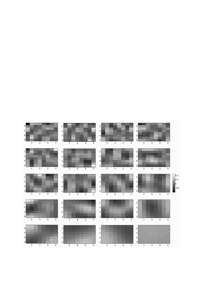
144 Chapter
4
compresseig.m
function [res]=compresseig(x)
x=double(reshape(x,1,64));
load TMEIG
res=TM*x';
________________________________________________________________________
decompresseig.m
function [res]=decompresseig(x)
load TMEIG
res=reshape(TM'*x,8,8);
________________________________________________________________________
Figure 4-4. Basis used for Ear Image Compression

4. Selected Applications
145
3.
ADAPTIVE NOISE FILTERING USING
BACKPROPAGATION NEURAL NETWORK
Consider the signal transmitted through the noisy channel gets corrupted
with the noise. The corrupted signal is given as the input to the FIR filter as
given below to filter the noisy part of the signal.
Let x(n) be the noisy corrupted input signal to the system, y(n) be the
output signal of the system which is the filtered signal and h(n) is the impulse
response of the system. They are related mathematically as given below.
y
(n) = x(n)*h(n)
⇒
N-1
y(n) =
Σ h(k)x(n-k)
k=0
‘*’ is the convolution operator. ‘N’ is the order of the filter. For
instance if the order of the filter is 11,
y(n) = h(0)x(n) + h(1)x(n-1) + h(2)x(n-2) + h(3)x(n-3) + h(4)x(n-4)+
…h(10) x(n-10)
The h(0), h(1), … h(10) are the impulse response of the system, otherwise
called as the filter co-efficients of the system.
Obtaining the values of the filter co-efficients is the task involved in
designing the digital filter to do specific operation. To obtain the values
there is the need to study about the nature of the noise of the channel.
In practical situations the reference signal is sent through the channel and
the corresponding corrupted signal obtained as the output of the channel is
stored. These are used for determining the filter co-efficients of the FIR
filter. Once filter co-efficients are obtained, they are used to filter the real
time noisy signal corrupted due to channel transmission at the receiver side.
Figure 4-5. FIR FILTER
146 Chapter
4
FIR Filter block as described above can also be replaced with the Back
propagation Neural Network block as mentioned in the chapter 1 to perform
filtering operation as described below. In this experiment the reference
signal and its corresponding corrupted signal are assumed to be known.
3.1
Approach
Step 1: Back propagation neural network (see chapter 1) is constructed with
11 input Neurons and 1 output neuron and 5 Hidden neurons (say)
Step 2: In signal processing point of view, input of the neural network is the
corrupted signal and the output of the neural network is the filtered
signal.
Step 3: During the training stage, the elements of the Input vectors are the
samples collected from the corrupted reference signal. Similarly
element of the output vector is the corresponding sample collected
from the reference signal.
Figure 4-6.
BPNN
Filter
Structure

4. Selected Applications
147
The Hetero association table relating the sample input vector and the
corresponding output vector used for training the constructed ANN is given
below. Note that x is the corrupted reference signal and y is the reference
signal
Step 4: Train the Artificial Backpropagation Neural Network as described
in the chapter 1. Store the Weights and Bias.
Step 5: Now the BPNN filter is ready to filter the original corrupted signal.
3.2
M-file for Noise Filtering Using ANN
_______________________________________________________
noisefiltuanngv.m
%Noise filtering using ANN
A=wavread('C:\Program Files\NetMeeting\Testsnd');
B=A(:,2);
B=B(6001:1:7000,1);
B=B';
B=(B+1)/2;
Table 4-1. Sample Hetero Association table relating input vectors and output vectors
x1 x2 x3 x4 x5 x6 x7 x8 x9 x10 x11 Y
X(10) X(9) X(8) X(7) X(6) X(5) X(4) X(3) X(2) X(1) X(0) Y(0)
X(11) X(10) X(9) X(8) X(7) X(6) X(5) X(4) X(3) X(2) X(1) Y(1)
X(12) X(11) X(10) X(9) X(8) X(7) X(6) X(5) X(4) X(3) X(2) Y(2)
…
X(16) X(15) X(14) X(13) X(12) X(11) X(10) X(9) X(8) X(7) X(6) Y(16)
X(17) X(16) X(15) X(14) X(13) X(12) X(11) X(10) X(9) X(8) X(7) Y(17)
X(18) X(17) X(16) X(15) X(14) X(13) X(12) X(11) X(10) X(9) X(8) Y(18)
X(19) X(18) X(17) X(16) X(15) X(14) X(13) X(12) X(11) X(10) X(9) Y(19)
X(20) X(19) X(18) X(17) X(16) X(15) X(14) X(13) X(12) X(11) X(10) Y(20)
…
of the BPNN

148 Chapter
4
%Assumed channel characteristics which is disturbing the signal.
H=[0.7071 -0.7071];
C=conv(H,B);
%Collections
INPUTVECTOR=[ ];
OUTPUTVECTOR=[ ];
for i=1:1:5000
x=round(rand*(100-12))+1;
INPUTVECTOR=[INPUTVECTOR;C(x:1:x+10)];
OUTPUTVECTOR=[OUTPUTVECTOR;B((x+11))];
end
W1=rand(5,11);
B1=rand(5,1);
W2=rand(1,5);
B2=rand(1,1);
nntwarn off
[W1,B1,W2,B2]=trainbpx
(W1,B1,'logsig',W2,B2,'logsig',INPUTVECTOR',OUTPUTVECTOR',[250 100000 0.02
0.01]);
save WEIGHTSNOISEFILT W1 B1 W2 B2
D=blkproc(C,[1 1],[0 5],'dofilter(x)');
D=(D-0.5)*2;
figure
subplot(3,1,1)
plot(B)
title('Original signal')
subplot(3,1,2)
plot(C)
title('Corrupted signal')
subplot(3,1,3)
plot(D)
title('Retrieved signal')
_________________________________________________________
4. Selected Applications
149
________________________________________________________________________
dofilter.m
function [res]=dofilter(x)
load WEIGHTSNOISEFILT
res=simuff(x',W1,B1,'logsig',W2,B2,'logsig');
3.3
Program Illustration
Figure 4-7 Noise Filtering using BPNN
Note that low frequency information is lost and that is not retrieved in the
filtered signal. This is due to the fact that first 100 samples are used to train
the ANN. If the training sequence is increased, low frequency information
can also be preserved in the filtered signal. Also note that MATLAB Neural
Network toolbox is used to train the network.
________________________________________________________________________
150 Chapter
4
4.
BINARY IMAGE ROTATION USING
TRANSFORMATION MATRIX
Figure 4-8. Vector basis for Binary Image Rotation
Consider the vector space spanned by the basis [1 0]
T
and [0 1]
T
.
Transformation of the vector [1 0] is the vector [0.7071 0.7071] that is in
the same space. Transformed vector is represented as the linear
combination of the basis [1 0]
T
and [0 1]
T
with vector co-efficient 0.7071
and 0.7071 respectively. Similarly the transformation of the vector [0 1]
T
is
the vector [-0.7071 0.7071] that is in the same space.
The transformed vector [-0.7071 0.7071] is represented as the linear
combination of the basis [1 0]
T
and [0 1]
T
with co-efficient –0.7071 and
0.7071 respectively.
The transformation described above rotates the vector counter clockwise
by 45
0
as mentioned in the figure 4-7.
Thus the transformation matrix used to rotate the vector counter
clockwise by 45
0
is computed using the method described in the chapter 3 is
given below.
0.7071 0.7071
0.7071 -0.7071
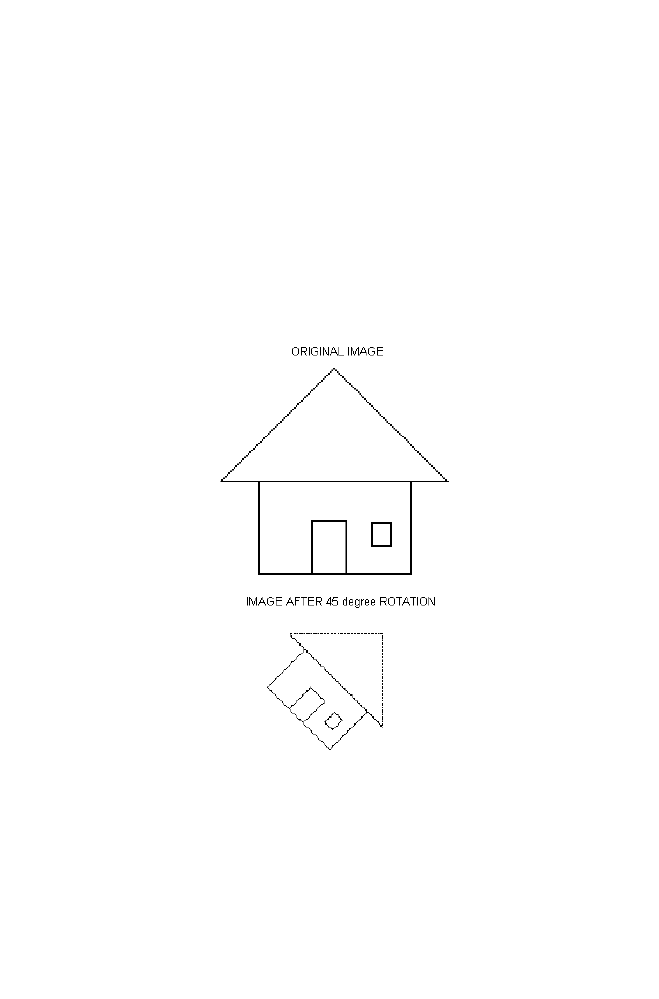
4. Selected Applications
151
4.1
Algorithm
Step 1: Read the Binary image.
Step 2: Find the position vectors of the black pixels of the Binary image.
Step 3: Transform the position vectors using the transformation matrix to
obtain the new sets of positions.
Step 4: Create the blank image completely filled up with white pixels. Fill
the selected pixels of the blank image described by the positions
obtained in step 3 with black to obtain the rotated image.
Figure 4-9. Binary Image Rotation

152 Chapter
4
4.2
M-program for Binary Image Rotation
with 45 Degree Anticlockwise Direction
___________________________________________________________
binimrotationgv.m
A=imread(selectfig8','bmp');
TM=[0.7071 0.7071;-0.7071 0.7071];
[X Y]=find(A==0);
VECT=[X Y];
TRANSVECT=TM*VECT';
TRANSVECT=round(TRANSVECT-min(min(TRANSVECT))+1);
m=max(max(TRANSVECT));
B=ones (m, m);
for k=1:1:length(TRANSVECT)
B(TRANSVECT(1,k),TRANSVECT(2,k))=0;
end
figure
subplot(2,1,1)
imshow(A)
title('ORIGINAL IMAGE')
subplot(2,1,2)
imshow(B)
title('IMAGE AFTER 45 degree ROTATION')
___________________________________________________________
5.
CLUSTERING TEXTURE IMAGES USING
K-MEANS ALGORITHM
To retrieve the similar images from the database, sample image looking like
the same is used as the key. The low level features extracted from the key
image is used as the index for searching. So the data base has to be
maintained based on the low level feature vectors derived from the images.

4. Selected Applications
153
Consider 23 texture images are stored in the database. They are indexed
using the low level features collected from the image itself, so that 23 texture
images are stored under 4 categories. K-means algorithm is used to classify
the collected texture into 4 categories so that each image in the database is
associated with the number indicating the category. (i.e.) 1 indicates first
category, 2 indicates second category and so on. This is called texture
grouping and is done as described below.
5.1
Approach
Step 1: Every texture image in the database is divided into sub blocks of
size 8x8. The variance of every sub blocks are calculated. They are
arranged in the vector form of size 1x64. This is called Low-level
feature vector extracted from the image itself. Note that elements of
the low level feature vector can also be any other statistical
measurements measured from the image.
Step 2: The collected Low-level feature vectors are subjected to k-means
algorithm to classify the images into four categories as described in
the chapter 2
Step 3: Thus the index number is identified for every image in the database.
Also the centroids of the individual category are also stored. The
centroid is the vector which is of the same size as that of the feature
vector. [Refer chapter 2]
Step 4: To retrieve the images from the indexed database that looks like the
image which is given as the key image is described below.
• Extract the low level feature vector from the key image as described in
the step 1.
• Compute the Euclidean distance between the computed feature vector
and all the centroids corresponding to the individual category. The
category corresponding to smallest Euclidean distance is selected.
• All the images in that category is retrieved using the index number
associated with every images

154 Chapter
4
Figure 4-10. Texture images - Cluster 1
Figure
4
-11. Texture images - Cluster 2
Figure 4-12. Texture images - Cluster 3
Figure 4-13. Texture images - Cluster 4

4. Selected Applications
155
5.2
M – program for Texture Images Clustering
___________________________________________________________
patclasgv.m
for i=1:1:23
S=strcat(num2str(i),'.bmp');
temp1=rgb2gray(imread(S));
A{i}=temp1(1:1:40,1:1:48);
temp2=blkproc(A{i},[8 8],'var2(x)');
FEA{i}=reshape(temp2,1,size(temp2,1)*size(temp2,2));
end
FEAVECT=cell2mat(FEA');
P=kmeans(FEAVECT,4);
for i=1:1:4
figure
[x,y]=find(P==i);
for j=1:1:length(x)
subplot(1,length(x),j)
imshow(A{x(j)})
end
end
_________________________________________________________
var2.m
function [res]=var2(x)
res=var(reshape(x,1,64));

156 Chapter
4
6.
SEARCH ENGINE USING INTERACTIVE
GENETIC ALGORITHM
Consider the small Image database stored with Low-level feature vectors
associated with every image. Low-level feature vector associated with every
image is the 1D vector whose elements are the statistical measurements like
variance, kurtosis, and higher order moments etc., computed from the sub
blocks of the image. Low-level feature vector associated with every image in
the database acts as the index for searching the particular image from the
database. Interactive Genetic algorithm based searching procedure is
described below.
6.1
Procedure
1. The front panel of the search engine consists of finite number of images
displayed. (Say 8 images) as shown in the figure given below.
2. The user is asked to assign the rank for the individual images. The value
ranges from 0 to100 based on the user’s interest. (i.e.) User assigns higher
Figure
4
-
14
. Sample front panel

4. Selected Applications
157
rank if user likes that image and expecting the similar images in the next
iteration.
3. 4 Images are selected from the 8 images using Roulette wheel selection
(Refer chapter 1) as described below.
• Let the rank values assigned for the eight images are represented as the
vector as given below.
[10 90 10 10 10 90 10 90]
• Normalized vector is computed as
[0.0313 0.2813 0.0313 0.0313 0.03133 0.2813 0.0313 0.2813]
• Simulate Roulette wheel
Cumulative summation of the above-normalized vector is displayed below.
[0.0313 0.3125 0.3438 0.3750 0.4063 0.6875 0.7188 1]
Random number is generated as ‘r’. If r is in between ‘a’ and ‘b’ in the
cumulative summation vector song corresponding to the value ‘b’ is selected
as mentioned below.
Generated random number = 0.9501(say)
Therefore select 8
th
image.
Generated number =0.2311(say)
Therefore select 2
nd
image.
Similarly.
0.6068-----------------------------------6
th
image
0.0185-----------------------------------1
st
image.
4. Thus the selected images are 8,2,6,5
5. Low level features corresponding to the image number 8,2 6 and 5 are
computed. The vectors thus obtained are randomly chosen and is
subjected to cross over and mutation operation as described below.
Low level feature (LLF) vector before and after crossover
Vector 1 = [a b c d e f]

158 Chapter
4
Vector 2 = [A B C D E F] (say)
Note that the number of elements shown in the vector is considered as 6.
[Actually the size of the vector is around 200]
Low level feature (LLF) vector after crossover
Vector 1’= [a b c d E F]
Vector 2’ = [A B C D e f]
6. Thus 8 Low level feature vectors for the second generation are obtained
as mentioned below.
LLF1, LLF2, LLF3, LLF4, LLF5, LLF6, LLF7 and LLF8 (say)
7. Compute the Euclidean distance between the feature vector LLF1 with
all the low level feature vectors in the database. Retrieve the image
corresponding to the LLF vector in the database whose Euclidean
distance is smallest. Repeat the procedure for the feature vectors
LLF2, LLF3, … LLF8
9. Repeat the step from 1 to 8 until the user is satisfied with the images
obtained in the latest iteration.
6.2
Example
Consider the Image database consists of 94 Natural sceneries. Every image
is truncated to the standard size 200x200. The feature vector for the
particular image is computed as described below.
The image is divided into sub blocks of size 50x50 with overlapping size
of 8x8.The first feature namely variance of the histogram of the hue content,
are computed for the all the overlapping sub blocks of the image. This is
treated as first part of the feature vector corresponding to the image.
Similarly other features are computed for all the overlapping sub blocks of
the image to obtain other parts of the feature vector. All the parts belonging
to the individual features are combined to obtain the feature vector
corresponding to that particular image.
Thus feature vectors are computed for all the images in the data base.
8. Thus the image selected for the next iteration is listed below.
9, 4,
3, 13, 18, 45, 43 (say). Note that 9 in the selected list indicates
th
16,
9 image in the database.
4. Selected Applications
159
6.2.1
List of low level features computed in every sub blocks
1. Variance of the histogram of the hue content of the particular subblock is
computed.
2. Measurement of uniformity
p(z
i)
is the probability of gray value z
i
in the particular sub block of the
image
.
The uniformity of sub block of the image is measured using the
formula given below.
3. Measurement of Average Entropy
Average entropy is computed as described below.
4. Measurement of Relative smoothness
where,
σ(z
) is the standard deviation of the gray values z in the
particular sub block of the image.
5, 6, 7, 8. Variance of the approximation Wavelet co-efficient
The image is subjected to discrete wavelet transformation (DWT) to
obtain approximation co-efficient (app), horizontal detail co-efficient (hor),
vertical detail co-efficient (ver) and diagonal (both horizontal and vertical)
detail co-efficient(dia) The variance of the approximation co-efficient ‘app’
is computed and considered as 5
th
feature. Similarly the variance of the detail
co-efficient ‘hor’,’ver’ and ‘dia’ are considered as the 6
th
, 7
th
and 8
th
features
respectively.
of the image
160 Chapter
4
9. Skewness
The Skew ness of the gray values is computed for every sub block of
the image as mentioned below.
10. Kurtosis
The Kurtosis of the gray values is computed for every sub block of the
image as mentioned below.
6.3
M-program for Interactive Genetic Algorithm
__________________________________________________________
igagv.m
r=round(rand(1,8)*94);
figure
for k=1:1:8
subplot(4,2,k)
title('Assign the rank')
s=strcat(num2str(r(k)),'.jpg');
A=imread(strcat('E:\Naturepix\',s));
imshow(A)
title(strcat('Image',num2str(k)));
end
for iter=1:1:10
s1=input('Enter the rank for image 1(Between 0 to 100)');
s2=input('Enter the rank for image 2(Between 0 to 100)');
s3=input('Enter the rank for image 3(Between 0 to 100)');
s4=input('Enter the rank for image 4(Between 0 to 100)');

4. Selected Applications
161
s5=input('Enter the rank for image 5(Between 0 to 100)');
s6=input('Enter the rank for image 6(Between 0 to 100)');
s7=input('Enter the rank for image 7(Between 0 to 100)');
s8=input('Enter the rank for image 8(Between 0 to 100)');
vect=[s1 s2 s3 s4 s5 s6 s7 s8]/100;
normvect=vect/sum(vect);
c=cumsum(normvect);
u=[ ];
for i=1:1:4
r1=rand;
c2=c-r1;
[x,y]=find(c2>0);
if(y(1)==1)
u1=1
else
u1=y(1)-1
end
u=[u u1];
end
load NATUREFEATURE
for i=1:1:4
feature{i}=FEATURE(r(u(i)),:);
end
%Cross over to obtain 8 feature vectors
k=1;
for i=1:1:4
p1=round(rand*159)+1
r=round((rand*3)+1);
d1=feature{r};
r=round((rand*3)+1);
d2=feature{r}
nextfeature{k}=[d1(1:1:p1) d2(p1+1:1:160)];
k=k+1;
nextfeature{k}=[d1(1:1:p1) d2(p1+1:1:160)];
k=k+1;
end
r=[];
for l=1:1:8
n=nextfeature{l};
d=(FEATURE-repmat(n,94,1)).^2;
s=sum(d')

162 Chapter
4
[m1,n1]=min(s);
r=[r n1];
end
for k=1:1:8
subplot(4,2,k)
title('Assign the rank')
s=strcat(num2str(r(k)),'.jpg');
A=imread(strcat('E:\Naturepix\',s));
imshow(A)
title(strcat('Image',num2str(k)));
end
end
___________________________________________________________
igaimagegv.m
for i=1:1:94
s=strcat(num2str(i),'.jpg');
A=imread(strcat('E:\Naturepix\',s));
B{i}=naturefeature(A);
end
FEATURE=cell2mat(B');
save NATUREFEATURE FEATURE
_________________________________________________________
naturefeature.m
function [res]=naturefeature(x)
x=x(100:1:size(x,1),1:1:size(x,2)-100,:,:);
x=imresize(x,[200 200]);
y=rgb2hsv(x);
h=y(:,:,1);
res=blkproc(h,[32 32],[8 8],'huevar(x)');
res1=reshape(res,1,size(res,1)*size(res,2));
y=rgb2gray(x);
res=blkproc(y,[32 32],[8 8],'unif(x)');
res2=reshape(res,1,size(res,1)*size(res,2));
res=blkproc(y,[32 32],[8 8],'entropy(x)');
res3=reshape(res,1,size(res,1)*size(res,2));
res=blkproc(y,[32 32],[8 8],'relativesmooth(x)');
res4=reshape(res,1,size(res,1)*size(res,2));
res=blkproc(y,[32 32],[8 8],'wavelet(x)');

4. Selected Applications
163
res5=reshape(res,1,size(res,1)*size(res,2));
res=blkproc(y,[32 32],[8 8],'skew(x)');
res6=reshape(res,1,size(res,1)*size(res,2));
res=blkproc(y,[32 32],[8 8],'kurt(x)');
res7=reshape(res,1,size(res,1)*size(res,2));
res=[res1 res2 res3 res4 res5 res6 res7 ];
________________________________________________________
huevar.m
function [res]=huevar(x)
x=hist(reshape(x,1,size(x,1)*size(x,2),500);
res=var(x);
___________________________________________________________
unif.m
function [res]=unif(x)
z=reshape(x,1,size(x,1)*size(x,2));
h=hist(double(z),256);
h=h/sum(h);
res=sum(h.^2);
__________________________________________________________
entropy.m
function [res]=entropy(x)
z=reshape(x,1,size(x,1)*size(x,2));
h=hist(double(z),256);
h=h/sum(h);
res=(-1)*sum(h.*log2 (h+eps));
___________________________________________________________
relativesmooth.m
function [res]=relativesmooth(x)
z=reshape(x,1,size(x,1)*size(x,2));
res=1-(1/(1+var(z)));
___________________________________________________________

164 Chapter
4
wavelet.m
function [res]=wavelet(x)
x=double(x);
[c,l]=wavedec2(x,1,'db6');
a=appcoef2(c,l,'db6',1);
v1=var(reshape(a,1,size(a,1)*size(a,2)));
d1=detcoef2('h',c,l,1);
v2=var(reshape(d1,1,size(d1,1)*size(d1,2)));
d2=detcoef2('v',c,l,1);
v3=var(reshape(d2,1,size(d2,1)*size(d2,2)));
d3=detcoef2('d',c,l,1);
v4=var(reshape(d3,1,size(d3,1)*size(d3,2)));
res=[v1 v2 v3 v4];
_________________________________________________________
skew.m
function [res]=skew(x)
x=double(x);
z=reshape(x,1,size(x,1)*size(x,2));
h=hist(double(z),256);
h=h/sum(h);
m=mean(z);
res=sum(((z-m).^3).*h(z+1));
___________________________________________________________
kurt.m
function [res]=kurt(x)
x=double(x);
z=reshape(x,1,size(x,1)*size(x,2));
h=hist(double(z),256);
h=h/sum(h);
m=mean(z);
res=sum(((z-m).^4).*h(z+1));
_
__________________________________________________________

4. Selected Applications
165
6.4
Program Illustration
__________________________________________________________
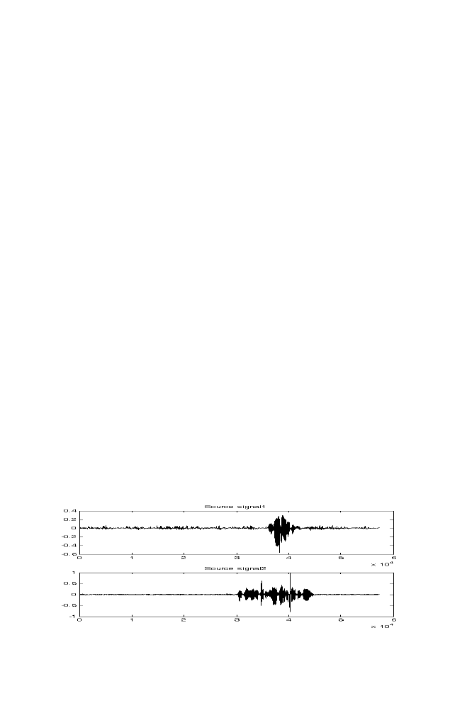
166 Chapter
4
7.
SPEECH SIGNAL SEPARATION AND DENOISING
USING INDEPENDENT COMPONENT ANALYSIS
Consider the two speakers talking in the meeting simultaneously with no
background noise. Two microphones are used for recording. One kept very
close to the first person. Another microphone is kept near to the second
person. The recorded signals of both the microphones can be treated as the
linear combinations of independent sources. [Two speech signals] Hence
ICA algorithm can be used to separate the two independent signals [Refer
chapter 2].
Consider the second situation in which single speaker is talking with the
background noise. Two microphones are used to record the signal. One
microphone kept near to the speaker. Another microphone kept near to the
assumed noise source. The recorded signals of both the microphones can be
treated as the linear combinations of independent sources [Speech signal +
Noise ].Similar to the above ICA algorithm can be used to separate the two
independent signals. Hence the ICA algorithm can be used to separate the
two independent signals and hence denoising is achieved.
7.1
Experiment 1
Two speech signals x1(t) and x2(t) are linearly mixed to get two mixed
signals y1(t) and y2(t) as given below.
y1(t)=0.7*x1(t) +0.3*x2(t)
y2(t)=0.3*x1(t)+0.7*x2(t)
The mixed signals are subjected to ICA algorithm. The independent
signals x1(t) and x2(t) are obtained as shown below. Note that FASTICA
toolbox is used to run the ICA algorithm.
Figure 4-15. Original speech signals
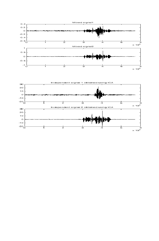
4. Selected Applications
167
Figure 4-16. Mixed signals
Figure 4-17 Separated speech signals using ICA
7.2
Experiment 2
Speech signal x(t) and noise n(t) are linearly mixed to get two mixed signals
y1(t) and y2(t) as given below.
y1(t) = 0.7*x(t) + 0.3*n(t)
y2(t) = 0.3*x(t)+ 0.7*n(t)
The mixed signals are subjected to ICA algorithm to obtain the speech
signal and noise signal separately.
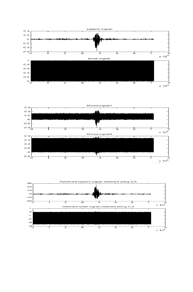
168 Chapter
4
Figure 4-18
Figure 4-19. Mixed signals
Figure 4-20. Retrieved speech and noise signals using ICA
. Speech signal and Noise signal before mixing

4. Selected Applications
169
7.3
M-program for Denoising
___________________________________________________________
noiseicagv.m
a=wavread('C:\MATLAB7\work\audio\revsam\ram1.wav');
b=rand(length(a),1);
m=min(length(a),length(b));
a=a(1:1:m);
b=b(1:1:m);
mixed1=0.7*a+0.3*b;
mixed2=0.3*a+0.7*b;
mixed=[mixed1'; mixed2'];
[signal]=fastica(mixed);
figure
subplot(2,1,1)
plot(mixed1)
title('Mixed signal1')
subplot(2,1,2)
plot(mixed2)
title('Mixed signal2')
figure
subplot(2,1,1)
plot(a)
title('speech signal')
subplot(2,1,2)
plot(b)
title('noise signal')
figure
subplot(2,1,1)
plot(signal(1,:))
title('Retrieved speech signal obtained using ICA')
subplot(2,1,2)
plot(signal(2,:))
title('Retrived noise signal obtained using ICA')
Note that the signal b(n) in the above program is another speech signal in
case of speech signal separation. The rests of the program remains same.

170 Chapter
4
8.
DETECTING PHOTOREALISTIC IMAGES
USING INDEPENDENT COMPONENT
ANALYSIS BASIS
The digital images captured using the camera are called as photographic
images and the images which are not captured using the camera are called as
photorealistic images. ICA basis are used in classifying the produced image
into photo graphic or photo realistic images as described below.
Figure 4-21
Figure 4-22. Sample photographic images
. Sample photo realistic images

4. Selected Applications
171
8.1
Approach
• The 10 photographic images and the 10 photo realistic images are
collected (see figure 4-3 and figure 4-4). The sub blocks of the image
sized 16x16 are randomly collected from both the categories. 500 sub
blocks are collected from photographic images and 500 subblocks are
collected from the photorealistic images.
• The subblock thus obtained is reshaped into the size 1x256. Auto
Regressive (AR) co-efficients of size 1x10 are obtained from the
reshaped subblock. This is repeated for all the collected sub blocks. The
set of AR vectors collected from photographic images and the photo
realistic images are subjected to ICA analysis and 10 ICA basis each of
size 1x10 are obtained. [Refer chapter 2]
• Every AR co-efficient vector obtained from the particular subblock of the
images is represented as the linear combination of 10 corresponding ICA
Basis. The co-efficient of the ICA basis are obtained using the inner
product of ICA basis with the corresponding AR co-efficients. This is
called feature e vector of that particular subblock of the image.
• Thus 500 feature vectors are collected from photographic images and the
500 feature vectors are collected from the photorealistic images. The
centroid of the feature vectors collected from the photographic images is
computed as C1. Similarly the centroid of the feature vectors collected
from the photo realistic images are computed as C2.
8.1.1
To classify the new image into one among the photographic
The image is divided into sub blocks. Feature vectors are extracted form
every sub blocks using ICA basis as described above. The Euclidean
distance between the feature vector obtained from the particular subblock
and the centroids ‘C1’ and ‘C2’ are computed as ‘d1’ and ‘d2’ respectively.
Assign the number 1 to that particular subblock if ‘d1’ is lowest Otherwise 2
is assigned to that subblock. This is repeated for all the sub blocks of the
image to be classified.
Count the number of ‘1’s and the number of ‘0’s assigned to the
subblocks of the image to be classified. If the number of 1’s is greater than
or photorealistic image

172 Chapter
4
0’s, decide that the image is photographic image. Otherwise the image is
classified as photo realistic image.
8.2
M-program for Detecting Photo Realistic Images
Using ICA Basis
___________________________________________________________
photorealisticdetgv.m
k=1;
for i=1:1:20
s=strcat('C:\Documents and Settings\user1\Desktop\Photorealistic\',num2str(i),'.jpg');
for j=1:1:50
temp=imread(s);
temp=rgb2gray(temp);
temp=temp(101:1:200,101:1:200);
r1=round(rand*(size(temp,1)-8))+1;
r2=round(rand*(size(temp,2)-8))+1;
temp=reshape(temp(r1:1:r1+7,r2:1:r2+7),1,64);;
temp=double(temp);
A{k}=lpc(temp,16);
k=k+1;
end
end
temp=cell2mat(A');
temp=temp(:,2:1:17);
I=fastica(temp);
save I I
k=1 ;
for i=1:1:20
s=strcat('C:\Documents and Settings\user1\Desktop\Photorealistic\',num2str(i),'.jpg');
for j=1:1:100
temp=imread(s);
temp=rgb2gray(temp);
temp=temp(101:1:200,101:1:200);
r1=round(rand*(size(temp,1)-8))+1;
r2=round(rand*(size(temp,2)-8))+1;

4. Selected Applications
173
temp=reshape(temp(r1:1:r1+7,r2:1:r2+7),1,64);
temp=double(temp);
temp=lpc(temp,16);
temp=temp(2:1:17);
a=[ ];
for n=1:1:size(I,1)
a= [a sum(temp.*I(n,:)) ];
end
feaext1{k}=a;
k=k+1;
end
end
FEA=cell2mat(feaext1');
C1=mean(FEA(1:1:1000,:));
save C1 C1
C2=mean(FEA(1001:1:2000,:));
save C2 C2
_______________________________________________________________________
phototest.m
for i=1:1:20
s=strcat('C:\Documents and Settings\user1\Desktop\Photorealistic\',num2str(i),'.jpg');
A=imread(s);
B=rgb2gray(A);
B=B(101:1:300,101:1:300);
imshow(B)
C=blkproc(B,[8 8],'assigncenno(x)');
if(length(find(C==1))>length(find(C==0)))
disp('The image is photorealistic image')
else
disp('The image is photographic image')
end
end
_______________________________________________________________________

174 Chapter
4
assigncenno.m
function [res]=assigncenno(x)
x=double(x);
load C1
load C2
load I
x=reshape(x,1,64);
p=lpc(x,16);;
temp=p(2:1:17);
a=[ ];
for n=1:1:size(I,1)
a= [a sum(temp.*I(n,:)) ];
end
d1=sum((C1-a).^2);
d2=sum((C2-a).^2);
if(d1<d2)
res=0;
else
res=1;
end
___________________________________________________________
8.3
Program Illustration

4. Selected Applications
175
9.
BINARY IMAGE WATERMARKING USING
WAVELET DOMAIN OF THE AUDIO SIGNAL
The process of hiding the information like text, binary image, audio etc. into
another signal source like image, audio etc. is called watermarking. The
approach involved in watermarking the binary image signal in the wavelet
domain of the audio signal is described in the example given below.
9.1
Example
Step 1: Consider the audio signal sampled with the sampling rate of 11025 Hz.
Step 2: The audio signal is divided into frames with 1024 samples. Decompose
every frame of the speech signal using ‘db4’ wavelet transformation
[See wavelet transformation in chapter 3]. Hide the first bit of the
binary data collected from the binary image into the third level detail
co-efficients obtained using wavelet decomposition of the first audio
frame. This is done by changing the values of the third level detail co-
efficients such that mean of the third level detail co-efficients is
modified to ‘m+k’ if the binary value is ‘1’ or to ‘m-k’ if the binary
value is ‘0’.Note that variance remains same.[See Mean and variance
normalization in Chapter 2]. The variable ‘m’ is the mean of the fifth
level detail co-efficients. The value for the constant ‘k’ is chosen as
1/5
th
of the energy of the third level detail co-efficients.
Step 3: This is repeated for the other frames of the speech signal for hiding
the entire bits obtained from the binary image.
Step 4: Thus Binary image is hidden in the wavelet domain of the audio
signal.
Step 5: The hidden binary data is retrieved by comparing the mean of the
corresponding detail co-efficients computed before and after hiding.
If the mean of the third level detail co-efficient of the particular
frame corresponding to the original signal is greater than the mean
of the third level detail co-efficients of the respective frame
corresponding to the watermarked signal, the bit stored is
considered as ‘1’,otherwise ‘0’.
Step 6: Note that the duration of the audio signal is chosen such that all the
binary data collected from the binary image are hidden in the audio
signal.

176 Chapter
4
In this example length of the audio signal used for hiding binary image
data is 11488 samples. It is repeated 100 times so that the length of the audio
signal becomes 1148800 samples. The size of the Binary image used is
45X45.Binary image is stored at the rate of 1 bit in 256 samples of the audio
signal.
9.2
M-file for Binary Image Watermarking
in the Wavelet Domain of the Audio Signal
___________________________________________________________
audiowatermarkdb4gv.m
A= wavread ('C:\WINDOWS\Media\Microsoft Office 2000\glass.wav');
A=repmat(A,100,1);
A=A';
len=fix(length(A)/256);
for k=1:1:len-1
temp=A((k-1)*256+1:1:(k-1)*256+256);
col{k}=daub4water(temp);
end
I=imread('BINIMAGE.bmp');
I=I(1:1:45,1:1:45);
I=reshape(I,1,45*45);
for k=1:1:length(I)
switch I(k)
case 0
temp=col{k}{2}{3};
e=sum(temp.^2)/5;
m=mean(temp);
v=var(temp);
col{k}{2}{3}=meanvarnorm(temp,(m-e),v);
case 1
temp=col{k}{2}{3};
e=sum(temp.^2)/5;
m=mean(temp);
v=var(temp);
col{k}{2}{3}=meanvarnorm(temp,(m+e),v);
end
end

4. Selected Applications
177
s=256;
signal=[];
for k=1:1:length(I)
approx=col{k}{1};
det=col{k}{2};
app=approx{log2(s)-2};
for i=(log2(s)-2):-1:1
a=[app;det{i}];
a=reshape(a,1,size(a,1)*size(a,2));
a=[ a(length(a)-1:1:length(a)) a];
app=createdaubinvmatrix(length(a)-2)*a';
app=app';
end
signal=[signal app];
end
figure
subplot(3,1,1)
plot(signal(1:1:5520));
title('Original signal')
subplot(3,1,2)
plot(A(1:1:5520),'r');
title('Watermarked signal');
subplot(3,1,3)
plot(signal(1:1:5520)-A(1:1:5520))
title('Difference signal')
save signal signal
_________________________________________________________
daub4water.m
function [res]=daub4water(x)
a=x;
s=length(a);
for i=1:1:log2(s) -2
a=[a a(1:2)];
temp=createdaubmatrix(length(a)-2)*a';
temp=temp(1:1:length(temp));
temp=reshape(temp,2,length(temp)/2);
approx{i}=temp(1,:);
det{i}=temp(2,:);
a=approx{i};

178 Chapter
4
end
res{1}=approx;
res{2}=det;
________________________________________________________________________
gethiddenimage.m
% size of the Binary hidden image is 45x45
A= wavread ('C:\WINDOWS\Media\Microsoft Office 2000\glass.wav');
A=repmat(A,100,1);
A=A';
len=fix(length(A)/256);
for k=1:1:len-1
temp=A((k-1)*256+1:1:(k-1)*256+256);
col1{k}=daub4water(temp);
end
load signal
A=signal;
len=fix(length(A)/256);
for k=1:1:len
temp=A((k-1)*256+1:1:(k-1)*256+256);
col2{k}=daub4water(temp);
end
temp=[];
for k=1:1:45*45
m1=mean(col1{k}{2}{3});
m2=mean(col2{k}{2}{3});
if(m1>m2)
temp=[temp 0];
else
temp=[temp 1];
end
end
temp1=reshape(temp,45,45);
figure
imshow(temp1);
______________________________________________________________________

4. Selected Applications
179
meanvarnorm.m
function [res]=meanvarnorm(a,md,vd)
m=mean(a);
v=sqrt(var(a));
vd=sqrt(vd);
delta=abs((a-m)*vd/v);
res=ones(1,length(a))*md;
[p]=quantiz(a,m);
p=p';
p=p*2-1;
res=res+p.*delta;
__________________________________________________________
createdaubmatrix.m
function [res]=createdaubmatrix(m)
a=[(1+sqrt(3))/(4*sqrt(2)) (3+sqrt(3))/(4*sqrt(2)) (3-sqrt(3))/(4*sqrt(2)) …
(1-sqrt(3))/(4*sqrt(2))];
b=[(1-sqrt(3))/(4*sqrt(2)) -(3-sqrt(3))/(4*sqrt(2)) (3+sqrt(3)) /(4*sqrt(2)) …
-(1+sqrt(3))/(4*sqrt(2))];
t1=repmat([a(2) b(3)],1,(m/2));
t2=repmat([a(3) b(4)],1,m/2);
t3=repmat([a(4) 0],1,m/2);
t4=repmat([b(1) 0],1,m/2);
res=diag(repmat([a(1) b(2)],1,m/2)) + diag(t1(1:1:m-1),1)+…
diag(t2(1:1:m-2),2)+diag(t3(1:1:m-3),3)+diag(t4(1:1:m-1),-1) ;
res=[res [zeros(1,m-2) res(1,3) res(2,3)]' [zeros(1,m-2) res(1,4) res(2,4)]'];
________________________________________________________________________
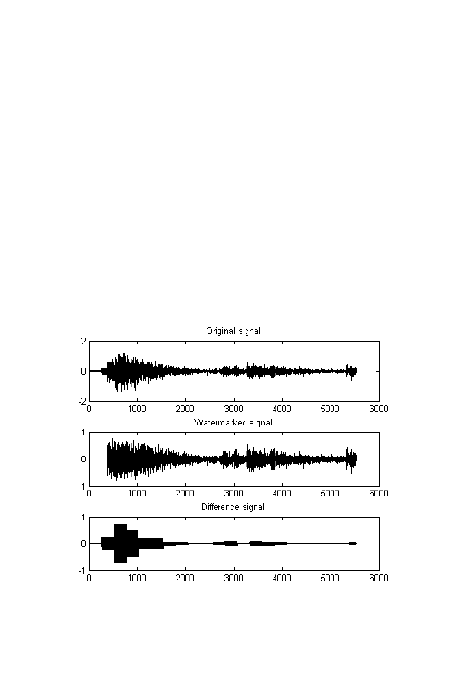
180 Chapter
4
______________________________________________________________________
createdaubinvmatrix.m
function [res]=createdaubinvmatrix(m)
a=[(1+sqrt(3))/(4*sqrt(2)) (3+sqrt(3))/(4*sqrt(2)) (3-sqrt(3))/(4*sqrt(2)) (1-sqrt(3))/(4*sqrt(2))];
b=[(1-sqrt(3))/(4*sqrt(2)) -(3-sqrt(3))/(4*sqrt(2)) (3+sqrt(3))/(4*sqrt(2)) -(1+sqrt(3))/(4*sqrt(2))];
t1=repmat([b(3) a(2)],1,(m/2));
t2=repmat([a(1) b(2)],1,m/2);
t3=repmat([b(1) 0],1,m/2);
t4=repmat([a(4) 0],1,m/2);
res=diag(repmat([a(3) b(4)],1,m/2)) + diag(t1(1:1:m-1),1)+ …
diag(t2(1:1:m-2),2)+diag(t3(1:1:m-3),3)+diag(t4(1:1:m-1),-1) ;
res=[res [zeros(1,m-2) res(1,3) res(2,3)]' [zeros(1,m-2) res(1,4) res(2,4)]'];
___________________________________________________
9.3
Program Illustration
Figure
4
-23. Audio signal before and after watermarking
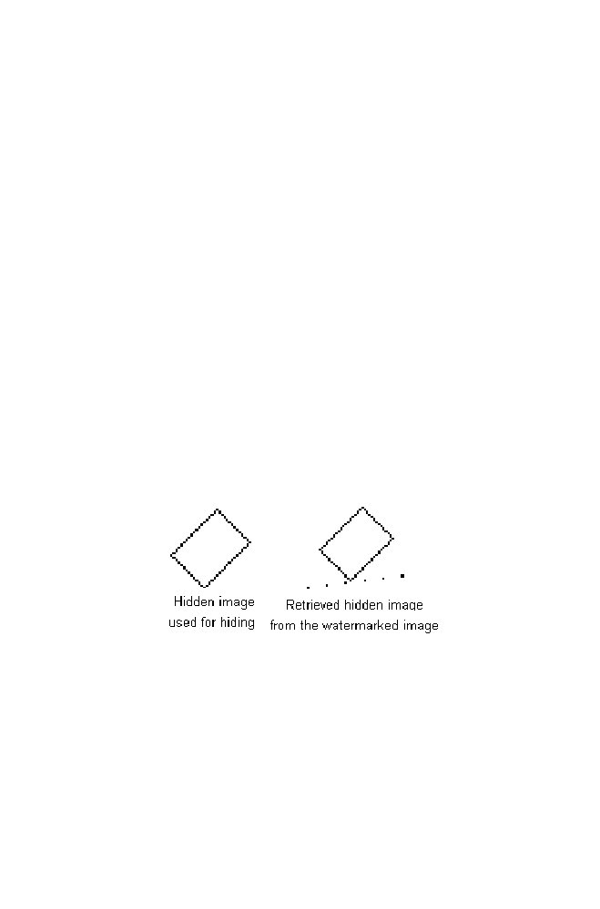
4. Selected Applications
181
Figure 4-24
Figure
4
-25. Hidden and Retrieved Binary image
. Original and watermarked signal in zoomed level

Appendix
List of Figures
Figure 1-1 PSO Example zoomed version
Figure 1-2 PSO Example
Figure 1-3 Vector Representation of PSO Algorithm
Figure 1-4 Roulette Wheel
Figure 1-5 Convergence of population
Figure 1-6 Illustration of simulated Annealing
Figure 1-7 Illustration of simulated Annealing 1
Figure 1-8 Illustration of simulated Annealing 2
Figure 1-9 Illustration of simulated Annealing 3
Figure 1-10 BPN Structure
Figure 1-11 ANN Algorithm Illustration
Figure 1-12 Illustration of SSE decreases with Iteration
Figure 1-13 Fuzzy system
Figure 1-14 Relationship between crisp value and Fuzzy membership
value for the variable X
Figure 1-15 Relationship between crisp value and Fuzzy membership
value for the variable Y
Figure 1-16 Relationship between crisp value and Fuzzy membership
value for the variable Z
Figure 1-17 Xinput as the crisp input for the variable X
Figure 1-18 Xinput as the crisp input for the variable Y
Figure 1-19 Defuzzification
183
Figure 1-20 Relationship between the crisp value and fuzzy membership
for the i nput variable X in the example

184 Appendix
Figure 1-21 Relationship between the crisp value and fuzzy membership
Figure 1-22 Relationship between the crisp value and fuzzy membership
Figure 1-24 Illustration of Ant colony
Figure 1-25 Matrix A (Ant colony)
Figure 1-26 Matrix B (Ant colony)
Figure 1-27 Iteration (vs) Best cost selected by the 4 ants
Figure 2-1 Clustering example with four clusters
Figure 2-2 Illustration of K-means algorithm
Figure 2-3 Data along with the final centroids obtained by k-means
algorithm
Figure 2-4 Illustration of Fuzzy k-means algorithm
Figure 2-5 Data and the final centroids obtained using Fuzzy k-means
algorithm
Figure 2-6 Illustration of change in the membership value in every
iteration
Figure 2-7 Illustration of Mean and Variance Normalization of the
speech
signal
Figure 3-1 Hotelling transformation for binary image rotation
Figure 3-2 Vector space along with Eigen vectors
Figure 3-3 Vector space after KLT and the corresponding eigen vectors
Figure 3-4 Projection Illustration
Figure 3-5 Projection of the vector on the plane
Figure 3-6 Gram-Schmidt Orthogonalization procedure
Figure 3-7 Original signal used for Haar decomposition
Figure 3-8 Approximation co-efficients obtained using Haar
transformation
Figure 3-9 Detail co-efficients obtained using Haar transformation
Figure 3-10 Illustration of Inverse Haar transformation
Figure 3-11 Original signal used for Daubechies 4 wavelet
decomposition
Figure 3-12 Approximation co-efficients at different levels
Figure 3-13 Detail co-efficients at different levels
Figure 3-14 Illustration of Inverse Daubechies 4 transformation
Figure 4-1 Sample Ear images before and after
normalization
Figure 4-2 Eigen Ears corresponding to the largest
Eigen values
for the i nput variable Y in the example
for the i nput variable Z in the example
Figure 1-23 Defuzzification in the example

Appendix
185
Figure 4-3 Ear image compression with the ratio 3.2:1
using Eigen basis
Figure 4-4 Basis used for Ear Image Compression
Figure 4-5 FIR Filter
Figure 4-6 BPNN Filter structure
Figure 4-7 Noise Filtering using BPNN
Figure 4-8 Vector basis forBinary Image Rotation
Figure 4-9 Binary Image Rotation
Figure 4-10 Texture images - Cluster 1
Figure 4-11 Texture images - Cluster 2
Figure 4-12 Texture images - Cluster 3
Figure 4-13 Texture images - Cluster 4
Figure 4-14 Sample Front panel
Figure 4-15 Original speech signals
Figure 4-16 Mixed signals
Figure 4-17 Separated speech signals using ICA
Figure 4-18 Speech signal and Noise signal before mixing
Figure 4-19 Mixed signals
Figure 4-20 Retrieved speech and noise signals using ICA
Figure 4-21 Sample photorealistic images
Figure 4-22 Sample photographic images
Figure 4-23 Audio signal before and after watermarking
Figure 4-24 Original and watermarked signal in zoomed level
Figure 4-25 Hidden and Retrieved Binary image
List of m-files
psogv.m
f1.m
geneticgv.m
fcn.m
sagv.m
minfcn.m
anngv.m
logsiggv.m
fuzzygv.m

antcolonygv.m
computecost.m
icagv.m
gmmmodelgv.m
clustercol.m
clusterno.m
kmeansgv.m
fuzzykmeansgv.m
meanvarnormgv.m
hotellinggv.m
gramgv.m
haartransgv.m
createhaarmatrix.m
haarinvtransgv.m
creatinvhaarmatrix.m
daub4trans.m
createdaubmatrix.m
daub4invtrans.m
createdaubinvmatrix.m
earpatgv.m
testinggv.m
earcompgv.m
compresseig.m
decompresseig.m
noisefiltanngv.m
dofilter.m
binimrotationgv.m
patclassgv.m
var2.m
18 Appendix
6

Appendix
187
igagv.m
igaimagegv.m
naturefeature.m
huevar.m
unif.m
entropy.m
relativesmooth.m
wavelet.m
skew.m
kurt.m
noiseicagv.m
photorealisticdetgv.m
phototest.m
assigncenno.m
audiowatermarkdb4gv.m
daub4water.m
gethiddenimage.m

Index
Adaptive noise filtering using
BPN, 145
Ant colony optimization, 44, 45, 48
Approximation co-efficients, 119,
121–123, 128, 129, 159
Artificial Genetic algorithm, 9
Average Entropy, 159
Binary image rotation, 150–152
BPN structure, 24
Chromosomes, 9, 11, 15–17
Clustering, 68, 69, 81, 152, 155
Clustering texture images, 152
Cost function of energy state, 18, 19
Covariance matrix, 56–60, 62, 68, 70,
72, 87–90, 141
Crisp value, 33–35, 38–40
Cross over, 9–11, 16, 17, 161
Daubechies-4 transformation, 127
Denoising, 166, 169
Detail co-efficients, 120–124,
127–130, 159, 175
Differential equation, 108
Ear image data compression, 141, 143
Ear pattern recognition, 135, 138
Eigen basis, 91, 92, 117, 141, 142
Eigen ear, 135–137
Eigen vectors, 88, 91–93, 103, 105,
106, 108, 118, 136, 141
Euclidean distance, 70, 136, 153,
158, 171
Expectation – maximization
algorithm, 70
Expectation stage, 71, 72
Exponential of matrix, 107
Fourier transformation, 113, 114
Fuzzy k-means algorithm, 79–83
Fuzzy logic systems, 32, 33
Fuzzy membership, 32–40
Gaussian Mixture Model, 68, 72
Global minima, 20, 21, 25
Gram-Schmidt orthogonalization
procedure, 100–103
Haar transformation, 120–124,
127, 128
Hotelling transformation, 87–90
Independent component analysis, 53,
65, 166, 170
Interactive genetic algorithm, 156, 160
Intersection, 32, 36
k-means algorithm, 77–83, 152, 153
Kurtosis, 54–56, 60, 156, 160
189

Local minima, 20, 21
Logsig, 25, 29, 31, 32, 148, 149
Low-level features, 152, 153,
156–159
Maximization stage, 71, 72
Mean and variance normalization,
84–86
Minima location of the function, 119
Mutation, 9–11, 157
Orthonormal basis, 91, 101, 102, 113,
115, 118
Orthonormal vectors, 100–102
Particle swarm optimization algorithm
(PSO), 1
Pheromone matrix, 46–48
Photographic images, 170–172
Photorealistic images, 170, 171
Positive definite matrix, 119
Powers of matrix, 103
Projection Matrix, 95, 97–99
Pseudo inverse of matrix, 109, 110
Relative smoothness, 159
Roulette wheel selection, 10, 11
Search engine, 156
Sequence, 104–106
Significant co-efficients, 102, 116
Simulated annealing, 18, 19, 23
Single Neuron Architecture, 25
Singular Value Decomposition (SVD),
93, 109
Skewness, 160
Speech signal separation, 166
SSE(Sum squared error), 28, 30
System stability test using Eigen
values, 118
Tansig, 25, 29
Transformation matrix, 112–118,
121, 122, 127, 142, 150
Uniformity, 159
Union, 32, 37
Vector space, 91, 92, 96, 97, 100,
101, 113–115, 117, 141,
142, 150
Watermarking, 175, 176
Wavelet basis, 117, 118
1
90
I ndex
Document Outline
- cover-image-large.jpg
- front-matter.pdf
- fulltext_001.pdf
- fulltext_002.pdf
- fulltext_003.pdf
- fulltext_004.pdf
- back-matter.pdf
Wyszukiwarka
Podobne podstrony:
Algorithm Collections for Digital Signal Processing Applications using Matlab E S Gopi
Digital Signal Processing Teil 4
Digital Signal Processing Teil 1
Digital Signal Processing Teil 3
Digital Signal Processing Teil 2
Optimization of injection molding process parameters using sequential simplex algorithm
using uml for modeling a distributed java application 1997
(ebook pdf) Mathematics Statistical Signal Processing WLBIFTIJHHO6AMO5Z3SDWWHJDIBJQVMSGHGBTHI
Inverter For Domestic Fuel Cell Applications
1Introduction Signal Processing Haslerid 19014 (2)
Next Gen VoIP Services and Applications Using SIP and Java
A Plastic Injection Molding Process Characterisation Using Experimental Technique (Jtdis41a01)
Developing your STM32VLDISCOVERY application using the MDK ARM
Developing your STM32VLDISCOVERY application using the Atollic TrueSTUDIO
Alpine PXA H600 Digital Phase Processor Instal
Are Evolutionary Rule Learning Algorithms Appropriate for Malware Detection
więcej podobnych podstron