MODFLOW 2000 Ref Manual OFR 00 92

MODFLOW-2000, THE U.S. GEOLOGICAL SURVEY MODULAR
GROUND-WATER MODEL—USER GUIDE TO MODULARIZATION
CONCEPTS AND THE GROUND-WATER FLOW PROCESS

By Arlen W. Harbaugh

, Edward R. Banta

, Mary C. Hill

, and

Michael G. McDonald

U.S. GEOLOGICAL SURVEY

Open-File Report 00-92

Reston, Virginia

2000

U.S. Geological Survey, Reston, VA

U.S. Geological Survey, Lakewood, CO

McDonald Morrissey Associates, Reston, VA

U.S. DEPARTMENT OF THE INTERIOR

BRUCE BABBITT, Secretary

U.S. GEOLOGICAL SURVEY

Charles G. Groat, Director

The use of trade, product, industry, or firm names is for descriptive purposes
only and does not imply endorsement by the U.S. Government.

For additional information write to:

Office of Ground Water
U.S. Geological Survey
411 National Center
Reston, VA 20192
(703) 648-5001

Copies of this report can be
can be purchased from:

U.S. Geological Survey
Branch of Information Services
Box 25286
Denver, CO 80225-0425

Preface

iii

PREFACE

This report describes an enhanced version of the U.S. Geological Survey modular ground-water model, called

MODFLOW-2000, for which the structure has been expanded to facilitate the solution of multiple related equations. The
performance of the program has been tested in a variety of applications. Future applications, however, might reveal errors
that were not detected in the test simulations. Users are requested to notify the U.S. Geological Survey of any errors found in
this User Guide or the computer program by using the address on the back of the report title page. Updates might
occasionally be made to both the User Guide and to MODFLOW-2000. Users can check for updates on the Internet at URL
http://water.usgs.gov/software/ground_water.html/.

Contents

CONTENTS

ABSTRACT................................................................................................................................................................................ 1

INTRODUCTION ...................................................................................................................................................................... 1

DESIGN CONCEPTS................................................................................................................................................................. 2

Previously Existing Design Concepts—Packages, Procedures, and Modules ..................................................................... 2

Added Design Concept—Processes..................................................................................................................................... 3

Overall Structure.................................................................................................................................................................. 4

Parameters and Variables..................................................................................................................................................... 4

Listing Output ...................................................................................................................................................................... 6

GLOBAL PROCESS .................................................................................................................................................................. 7

Activating Capabilities and Opening Files Using the Name File ........................................................................................ 7

Space Discretization............................................................................................................................................................. 7

Time Discretization.............................................................................................................................................................. 8

Units of Length and Time .................................................................................................................................................. 10

GROUND-WATER FLOW PROCESS.................................................................................................................................... 10

Ground-Water Flow Equation............................................................................................................................................ 10

Use of Parameters in the Ground-Water Flow Process...................................................................................................... 12

Layer Data and List Data ............................................................................................................................................ 12

Case 1: One Parameter Is Used to Determine a Cell Data Value ............................................................................... 13

Parameters for List Data ...................................................................................................................................... 13

Parameters for Layer Data ................................................................................................................................... 14

Case 2: Additive Parameters Are Used to Determine a Cell Data Value.................................................................... 16

Packages Included in this Report ....................................................................................................................................... 19

Previously Existing Packages ..................................................................................................................................... 19

Basic (BAS) Package........................................................................................................................................... 19

Block-Centered Flow (BCF) Package ................................................................................................................. 20

Horizontal Flow Barrier (HFB) package ............................................................................................................. 20

Source-Term Packages ........................................................................................................................................ 21

Head-Dependent Packages ............................................................................................................................. 21

Head-Independent Packages........................................................................................................................... 21

Time-Variant Specified-Head Package ............................................................................................................... 21

Solver Packages................................................................................................................................................... 21

New Package: Layer-Property Flow Package............................................................................................................. 22

Introduction ......................................................................................................................................................... 22

Basic Hydraulic Conductance Equations ....................................................................................................... 22

Horizontal Conductance................................................................................................................................. 25

Constant Product of Hydraulic Conductivity and Thickness within a Cell............................................. 25

Alternative Approaches for Calculating Horizontal Branch Conductances ............................................ 27

Vertical Conductance ..................................................................................................................................... 28

Vertical Flow Calculation Under Dewatered Conditions............................................................................... 31

Conversion from Dry to Wet.......................................................................................................................... 34

Storage Formulation....................................................................................................................................... 34

Storage Term Conversion............................................................................................................................... 35

Data Requirements ......................................................................................................................................... 38

Defining Layer-Data Variables ...................................................................................................................... 40

MODFLOW-96 to MODFLOW-2000 Data Conversion Program .................................................................................... 40

Adding Packages................................................................................................................................................................ 41

INPUT INSTRUCTIONS ......................................................................................................................................................... 41

Running MODFLOW-2000............................................................................................................................................... 42

Global Process Input Instructions ...................................................................................................................................... 43

Name File ................................................................................................................................................................... 43

Explanation of Variables in the Name File.......................................................................................................... 43

Discretization File....................................................................................................................................................... 45

Explanation of Variables Read from the Discretization File ............................................................................... 45

Multiplier File............................................................................................................................................................. 47

Explanation of Variables Read from the Multiplier File .................................................................................... 47

Example Multiplier Array Input Using the FUNCTION Keyword ..................................................................... 47

MODFLOW-2000—User Guide to Modularization Concepts and the

Ground-Water Flow Process

INPUT INSTRUCTIONS (Continued)

Global Process Input Instructions (Continued)

Zone File .....................................................................................................................................................................49

Explanation of Variables Read from the Zone File ..............................................................................................49

Ground-Water Flow Process Input Instructions .................................................................................................................50

Basic Package..............................................................................................................................................................50

Explanation of Variables Read by the BAS Package ...........................................................................................50

Output Control Option.................................................................................................................................................52

Output Control Using Words ...............................................................................................................................52

Explanation of Variables Read by Output Control Using Words.........................................................................53

Example Output Control Input Using Words .......................................................................................................54

Output Control Using Numeric Codes .................................................................................................................54

Explanation of Variables Read by Output Control Using Numeric Codes ..........................................................55

Block-Centered Flow Package ....................................................................................................................................56

Explanation of Variables Read by the BCF Package ...........................................................................................56

Layer-Property Flow Package .....................................................................................................................................59

Explanation of Variables Read by the LPF Package ............................................................................................60

Horizontal Flow Barrier Package ................................................................................................................................63

Explanation of Variables Read by the HFB Package ...........................................................................................63

River Package..............................................................................................................................................................65

Explanation of Variables Read by the RIV Package ............................................................................................65

Recharge Package........................................................................................................................................................67

Explanation of Variables Read by the RCH Package...........................................................................................67

Well Package ...............................................................................................................................................................69

Explanation of Variables Read by the WEL Package ..........................................................................................69

Drain Package..............................................................................................................................................................71

Explanation of Variables Read by the DRN Package ..........................................................................................71

Evapotranspiration Package ........................................................................................................................................73

Explanation of Variables Read by the EVT Package ...........................................................................................73

General-Head Boundary Package................................................................................................................................76

Explanation of Variables Read by the GHB Package ..........................................................................................76

Constant-Head Boundary Package ..............................................................................................................................78

Explanation of Variables Read by the CHD Package ..........................................................................................78

Strongly Implicit Procedure Package ..........................................................................................................................80

Explanation of Variables Read by the SIP Package .............................................................................................80

Slice-Successive Overrelaxation Package ...................................................................................................................81

Explanation of Variables Read by the SOR Package ...........................................................................................81

Preconditioned Conjugate-Gradient Package ..............................................................................................................82

Explanation of Variables Read by the PCG Package ...........................................................................................82

Direct Solver Package Input Instructions ....................................................................................................................84

Explanation of Variables Read by the DE4 Package............................................................................................84

Input Instructions for Array Reading Utility Modules........................................................................................................86

Explanation of Variables in the Array Control Records..............................................................................................86

Examples of Free-Format Control Records for Reading an Array ..............................................................................87

Input Instructions for List Utility Module (ULSTRD) .......................................................................................................88

Explanation of Variables Read by the List Utility Module .........................................................................................88

EXAMPLE ................................................................................................................................................................................89

Example Without Parameters .............................................................................................................................................89

Example With Parameters ................................................................................................................................................102

REFERENCES ........................................................................................................................................................................121

Contents

vii

FIGURES

1. Flowchart of Global, Ground-Water Flow, Observation, Sensitivity, and Parameter

Estimation Processes............................................................................................................................... 5

2. Finite-difference grid with plan view and cross section view ................................................................. 9

3. Prism of porous material illustrating Darcy’s law................................................................................... 23

4. Calculation of conductance through several prisms in series .................................................................. 24

5. Calculation of conductance between nodes by using transmissivities and dimensions of cells............... 25

6. Calculation of vertical conductance between two nodes ..................................................................... .... 29

7. Calculation of vertical conductance between two nodes with a semiconfining unit between.................. 30

8. Situation in which a correction is required to limit the downward flow into cell i,j,k+1, as a result

of partial desaturation of the cell............................................................................................ ................. 32

9. A model cell for which two storage factors are used during one time step ............................................. 37

10. Illustration of the system simulated in the example problem .............................................................. .... 89

11. LIST file for example problem without parameters ................................................................................ 93

12. GLOBAL file for example problem with parameters.............................................................................. 107

13. LIST file for example problem with parameters ..................................................................................... 113

MODFLOW-2000—User Guide to Modularization Concepts and the

Ground-Water Flow Process

viii

Introduction

MODFLOW-2000, The U.S. Geological Survey Modular Ground-Water
Model—User Guide to Modularization Concepts and the
Ground-Water Flow Process

By Arlen W. Harbaugh, Edward R. Banta, Mary C. Hill, and Michael G. McDonald

ABSTRACT

MODFLOW is a computer program that numerically solves the three-dimensional ground-water

flow equation for a porous medium by using a finite-difference method. Although MODFLOW was
designed to be easily enhanced, the design was oriented toward additions to the ground-water flow
equation. Frequently there is a need to solve additional equations; for example, transport equations and
equations for estimating parameter values that produce the closest match between model-calculated
heads and flows and measured values. This report documents a new version of MODFLOW, called
MODFLOW-2000, which is designed to accommodate the solution of equations in addition to the
ground-water flow equation. This report is a user’s manual. It contains an overview of the old and added
design concepts, documents one new package, and contains input instructions for using the model to
solve the ground-water flow equation.

INTRODUCTION

MODFLOW is a computer program that simulates three-dimensional ground-water flow through a porous

medium by using a finite-difference method (McDonald and Harbaugh, 1988). MODFLOW was designed to have
a modular structure that facilitates two primary objectives: ease of understanding and ease of enhancing. Ease of
understanding was an objective because U.S. Geological Survey technical managers generally believe that
modelers should understand how a model works in order to use it properly. Ease of enhancement was an objective
because experience showed that there was a continuing need for new capabilities. Examples of enhancements are
reports by Prudic (1989), Hill (1990), Leake and Prudic (1991), Goode and Appel (1992), Harbaugh (1992),
McDonald and others (1992), Hsieh and Freckleton (1993), Leake and others (1994), Fenske and others (1996),
and Leake and Lilly (1997).

MODFLOW was originally documented by McDonald and Harbaugh (1984). As with most computer

programs that are used over a long time period, MODFLOW underwent several overall updates. The second
version of MODFLOW is documented in McDonald and Harbaugh (1988), and this version is often called
MODFLOW-88 to distinguish it from other versions. A third version is called MODFLOW-96 (Harbaugh and
McDonald, 1996a and 1996b).

In addition to the enhancements and updates, the U.S. Geological Survey developed two major extensions to

MODFLOW—MODFLOWP (Hill, 1992) and MOC3D (Konikow and others, 1996). MODFLOWP and MOC3D
solve equations in addition to the ground-water flow equation. MODFLOWP solves a MODFLOW calibration
problem by calculating values of selected input data that result in the best match between measured and model
calculated values, and MOC3D solves the solute-transport equation for concentration.

Although MODFLOW was originally designed to facilitate change, its design concepts did not include

solving equations other than the ground-water flow equation. As a result, incorporating capabilities such as those
added through MODFLOWP and MOC3D was not as straightforward from the programmer’s or user’s

MODFLOW-2000—User Guide to Modularization Concepts and the

Ground-Water Flow Process

perspective as were the other enhancements that dealt only with the ground-water flow equation. Therefore,
MODFLOW-2000 has been developed to facilitate the addition of multiple types of equations. Ease of
understanding continues to be included as an objective of the design. There is also an objective to minimize
changes that would impact existing MODFLOW users.

For many data input quantities, MODFLOW-2000 allows definition using parameter values, each of which

can be applied to data input for many grid cells. In combination with new multiplication and zone array
capabilities, the parameters make it much easier to modify data input values for large parts of a model. Defined
parameters also can have associated sensitivities calculated and be modified to attain the closest possible fit to
measured hydraulic heads, flows, and advective travel. This is accomplished using the Observation, Sensitivity,
and Parameter-Estimation Processes of MODFLOW-2000, which are documented by Hill and others (2000).

This report first documents the enhanced modular structure that is incorporated within MODFLOW-2000 to

accommodate the solution of multiple equations. An overview of the new design concepts is provided from the
perspective of a user; the detailed design information needed by programmers will be provided in separate
documentation as the information becomes available. This report also documents the incorporation of the ground-
water flow equation within the new structure, including the documentation of a new package called the Layer-
Property Flow Package and input instructions for using MODFLOW-2000 to simulate ground-water flow. A user
will also need to refer to earlier MODFLOW reports, such as McDonald and Harbaugh (1988), to find
information about how the ground-water flow equation is solved by using the finite-difference method. The parts
of MODFLOW-2000 that solve additional equations also are documented in separate reports, such as Konikow
and others (1996) and Hill and others (2000).

Although some new data-input capabilities have been added to MODFLOW-2000, most of the input data

used by earlier versions of MODFLOW to simulate ground-water flow can be read without change. A data
conversion program is provided to convert the parts of the input data that require change.

DESIGN CONCEPTS

This section of the report discusses several general aspects of MODFLOW-2000. The first involves the old

and new modularization concepts and how they work together; these are presented in the first three sections
below. Next, MODFLOW-2000 allows system characteristics to be defined by using parameters, and the basic
ideas behind this change are discussed. Finally, a basic change in the major output files is discussed.

Previously Existing Design Concepts—Packages, Procedures, and Modules

MODFLOW-2000 expands upon the modularization approach that was originally included in MODFLOW

(McDonald and Harbaugh, 1988). The design of MODFLOW can be viewed from two perspectives. The first
perspective is the user’s perspective. A user views the program according to its capability to simulate different
kinds of ground-water flow problems. To facilitate this perspective, the program is divided into pieces called
packages. Each hydrologic capability, such as leakage to rivers, recharge, and evapotranspiration, that is included
within the ground-water flow equation is a separate package. Further, because there are many methods for solving
the simultaneous equations resulting from the finite-difference method, each solution method is a package. The
Preconditioned Conjugate Gradient (PCG2 of Hill, 1990) and Strongly Implicit Procedure (SIP) are examples of
solution methods implemented as packages in MODFLOW. Finally, the remainder of the code that is not included
in a hydrologic or solution package becomes the Basic (BAS) Package. BAS provides overall program control.

The second perspective is the perspective of the programmer, for whom the goal is to break the program into

pieces that make the program logic as simple as possible while maintaining the desired functionality. In
MODFLOW, these pieces are called procedures. The program logic, which is typically represented by a
flowchart, is thus represented by describing the sequence of procedures. Examples of procedures are the Read and
Prepare Procedure in which user-specified data are read and prepared for use and the Formulate Procedure in
which the finite-difference equation is constructed for each model cell.

Design

Concepts

To make it possible to divide easily the program into both packages and procedures as desired, the program

code is broken into smaller pieces called modules. Each module contains the program code within a single
procedure for a single package. The code for a package can therefore be created by collecting all of the modules
that correspond to the package. Likewise, the code for any procedure can be created by collecting all of the
modules that correspond to the procedure. The MAIN program creates the required procedural view of the
program by invoking the various modules in the proper procedural sequence. New packages can thus be added to
MODFLOW by providing the new modules and modifying the MAIN program to invoke the new modules in the
proper procedural sequence.

In summary, there are three modularization entities in all the earlier versions of MODFLOW: procedures,

packages, and modules. The module is the most fundamental entity. Modules can be grouped according to
packages or procedures in order to obtain the user’s or programmer’s perspective, respectively.

Added Design Concept—Processes

To incorporate the solution of multiple related equations, a fourth modularization entity called a process is

added. A process is a part of the code that solves a fundamental equation by a specified numerical method. For
example, the solution of the ground-water flow equation using the finite-difference method, which is the original
MODFLOW, is now called the Ground-Water Flow (GWF) Process. The GWF Process includes all aspects of
solving the flow equation, including the formulation of the finite-difference equations, data input, solving the
resulting simultaneous equations, and data output. If a different method, the finite-element method for example,
were used, then this would become a separate process. Note that the solution of the set of simultaneous equations
within the GWF Process is not a process. Rather, this is only one part of the broader process of solving the
ground-water flow equation by using the finite-difference method. Accordingly, as previously mentioned, there
are several solver packages that can be used to solve the simultaneous equations, and these are all considered to be
part of the GWF Process.

The Ground-Water Transport (GWT) Process (formerly referred to as MOC3D) is an example of another

process. The GWT Process solves the solute-transport equation as described by Konikow and others (1996) by
using the numerical method known as the method of characteristics. As with the ground-water flow equation,
there are many numerical methods that can be used to solve the solute-transport equation. A fundamentally
different method would be implemented as a separate process. Variants of the method of characteristics could be
incorporated as part of the GWT Process. Model calibration as implemented by Hill and others (2000) requires
three processes in addition to the GWF Process. The Observation (OBS) Process calculates simulated values that
are to be compared to measurements, calculates the sum of squared, weighted differences between model values
and observations, and calculates sensitivities related to the observations. The Sensitivity (SEN) Process solves the
sensitivity equation for hydraulic heads throughout the grid, and the Parameter-Estimation (PES) Process solves
the modified Gauss-Newton equation to minimize an objective function to find optimal parameter values.

All processes are divided into packages, procedures, and modules in the same way as in previous versions of

MODFLOW. Therefore, in MODFLOW-2000 a module has three levels of identification— process, package, and
procedure. The procedures within a process must be defined as required to program that process efficiently, and
there need be no commonality of procedures among processes. When procedures of two or more processes are
similar, however, there is some benefit from choosing the same procedure name. The naming convention selected
for MODFLOW-2000 requires that packages that are represented in multiple processes use the same package
name. For example, the modules in the Sensitivity Process that deal with river seepage using the River (RIV)
Package of the Ground-Water Flow Process must be designated as the RIV Package of the Sensitivity Process.

It is assumed that every non-Ground-Water Flow Process within MODFLOW-2000 operates with the

Ground-Water Flow Process. There is no assumption, however, that all the non-Ground-Water Flow processes
work together. For example, the Parameter-Estimation Process by Hill and others (2000) does not work with the
GWT Process. The documentation for each process should define the other processes with which it is compatible.

In addition to processes that solve equations, MODFLOW-2000 has the Global Process (GLO), which

controls overall program operation and sets up data structures that can be used by all processes. Some of the
initialization parts of the original MODFLOW have been put into the Global Process so that the Ground-Water

MODFLOW-2000—User Guide to Modularization Concepts and the

Ground-Water Flow Process

Flow Process is somewhat different in detail from the original MODFLOW. This is indicated in the MODFLOW-
2000 flowchart presented in the next section.

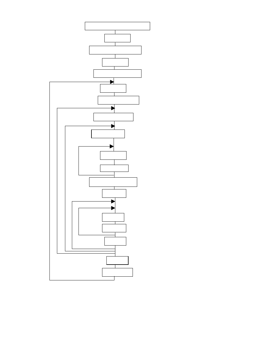
Overall Structure

Depending on what processes are included along with the Ground-Water Flow Process, MODFLOW’s

structure can be significantly more complex than it was originally. For example, when the Observation,
Sensitivity, and Parameter-Estimation Processes are added, a new parameter estimation loop is added to the
structure, which allows the Ground-Water Flow Process to be executed multiple times, and a new parameter-
sensitivity loop is added. A simplified flowchart of the Global, Ground-Water Flow, Observation, Sensitivity, and
Parameter-Estimation Processes combined is shown in figure 1. To illustrate the changes compared to the
original, the procedures and program loops of the Global and Ground-Water Flow Processes, which comprise the
functionality of the original MODFLOW, are identified with asterisks. Normally, each procedure would be shown
as a separate box; however, some of the sequential procedures are combined into a single box to save space in the
illustration. Further, figure 1 excludes some of the less important procedures of the Observation, Sensitivity, and
Parameter-Estimation Processes to minimize the size and complexity of the illustration. Enough of the structure is
shown to illustrate the expansion that is typical when using multiple processes.

Most of the procedures listed in figure 1 are described by McDonald and Harbaugh (1988). A new procedure

required by the Parameter-Estimation Process is Rewind (RW). The Rewind Procedure is needed to allow the
ground-water flow equation to be solved multiple times without totally redefining the way that the Ground-Water
Flow Process reads and stores data. This procedure rewinds the input files to their beginning before restarting the
Ground-Water Flow Process. Thus, the input files are reread each time the flow equation is solved.

Parameters and Variables

Another change in MODFLOW-2000 is the addition of parameters as used in parameter-estimation

terminology. In earlier MODFLOW documentation, the term parameter was generally used to mean any input
data value. For example, the recharge flux at a cell is a parameter by this definition. However, a more restricted
definition of “parameter” is commonly used when dealing with statistical parameter-estimation theory (Draper
and Smith, 1998; Ott, 1993). To make it possible to smoothly incorporate parameter estimation into MODFLOW-
2000 and provide an additional, convenient approach for specifying input data, the more restricted meaning is
used in this report. Thus, here a parameter is a single value that is given a name and determines the value of a
variable used in the finite-difference ground-water flow equation at one or more model cells. The definition of a
parameter specifies which variable is being defined and the cells for which the parameter applies. For example, a
parameter might define the aquifer hydraulic conductivity for a group of cells in a model layer, or a parameter
might define the riverbed conductance for one or more reaches of a river. Parameters are defined as part of the
Ground-Water Flow Process of MODFLOW-2000, and they can be used by other processes. In addition to
facilitating the incorporation of the Observation, Sensitivity, and Parameter-Estimation Processes, the parameter
approach for model input can make data input easier. For a full explanation of how to define parameters, refer to
the Using Parameters in the Ground-Water Flow Process Section of this report.

In order to be consistent with this new usage of the term “parameter” in MODFLOW-2000, the term

“auxiliary parameter” as used in MODFLOW-96 (Harbaugh and McDonald, 1996a, p. 26) has been changed to
“auxiliary variable.”

Design

Concepts

GWF FM*

GWF AP*

GWF OC*, BD*, OT*

STRESS LOOP*

ITERATION LOOP*

PES AP

SEN FM

SEN AP

ITERATION LOOP

PARAMETER-ESTIMATION
LOOP

TIME STEP LOOP*

GWF AD*

PARAMETER-
SENSITIVITY LOOP

GWF ST* and RP*

GWF AL* and RP*

GWF AL

GLO DF*, AL*, and RP*

OBS, SEN, and PES AL

OBS, SEN, and PES RP

PES RW

OBS FM

SEN OT

PES OT

GWF RP

Figure 1. -- Flowchart of Global (GLO), Ground-Water Flow (GWF), Observation (OBS),
Sensitivity (SEN), and Parameter Estimation (PES) Processes.

Procedures:

DF -- Define

AL -- Allocate

RP -- Read and Prepare

RW -- Rewind

ST -- Stress

AD -- Advance a time step

FM -- Formulate equations

AP -- Solve equations

OC -- Output Control

BD -- Calculate volumetric
budget

OT -- Write output

* Indicates procedures that comprise
the functionality of the original
MODFLOW.

MODFLOW-2000—User Guide to Modularization Concepts and the

Ground-Water Flow Process

Listing Output

Earlier versions of MODFLOW always produced a file called the listing file. With the addition of the

Parameter-Estimation Process, in which the parameter-estimation loop (fig. 1) may be repeated several times
during the estimation of parameters, the potential for excessively long output files arises. During each parameter-
estimation iteration, the Ground-Water Flow Process executes and produces written output related to one
simulation of the ground-water flow problem, and the Sensitivity Process executes and produces written output
related to each parameter considered. If all this output is written to a single file, then that file will increase in size,
possibly dramatically, with each iteration of the Parameter-Estimation Process. In most cases, during parameter
estimation, results of intermediate simulations are of little or no interest, and the output from these simulations is
unneeded.

To provide users with the option to retain only the output of most interest and limit the amount of output

generated, MODFLOW-2000 can produce either one or two listing output files. When the user specifies that one
output file is to be generated, all listing output from the model is written to that file. When the user specifies that
two output files are to be generated, output that applies to the overall model run is written to a file called the
GLOBAL file, but most of the output from Ground-Water Flow and Sensitivity Processes is written to a file
called the LIST file. Further, when a new iteration begins, the LIST file is erased and generated anew. As a result,
most of the output from the Ground-Water Flow and Sensitivity Processes is limited to that produced during the
most recently executed parameter-estimation iteration. Thus, the use of two files avoids generating excessively
large amounts of output.

If the Parameter-Estimation Process is not being used, the amount of output is the same when either one or

two output files are used because no process is executed more than once. However, two files can still be used in
this situation to divide the output into two pieces. This is a matter of user preference. If the Parameter-Estimation
Process is used, two output files are highly recommended. For additional information see Hill and others (2000).

As described in the Input Instructions Section of this report, the use of one or two listing files is determined

by which file types are defined in the name file. File types LIST and GLOBAL indicate that the respective listing
files are to be used (file type, as used for MODFLOW, is defined in the Activating Capabilities and Opening Files
Using the Name File Section of this report). If only one of these file types is specified in the name file, then all the
listing output is written to that file.

The rest of this section summarizes the contents of the GLOBAL and LIST files, with the assumption that the

user has specified that both GLOBAL and LIST files be created. The GLOBAL file contains information that
applies to the model run as a whole. Output from the Define (DF), Allocate (AL), and Read and Prepare (RP)
procedures of the Global, Observation, Sensitivity, and Parameter-Estimation Processes (fig. 1) is written to the
GLOBAL file. The output includes the names and types of all files that are opened. Input for the Global Process is
echoed to the GLOBAL file; this information includes a description of the spatial and temporal discretization to
be used. If the Observation, Sensitivity, or Parameter-Estimation Processes are being used, their input is echoed.
Input for the selected solver package is echoed. The GLOBAL file also shows the parameter definitions read from
the input files for the individual packages that are used to simulate various boundary conditions and stresses for
the Ground-Water Flow Process.

If the Observation Process is active, the GLOBAL file also contains information that is calculated during the

model run. If the Observation Process is active while the Sensitivity and Parameter-Estimation Processes are
inactive, summary information related to the fit of the model calculations to the observed values is written to the
GLOBAL file. If, in addition to the Observation Process, the Sensitivity Process is active, the GLOBAL file also
includes information that quantifies the sensitivity of the model-calculated equivalents of observations to the
parameter values. If, in addition to the Observation and Sensitivity Processes, the Parameter-Estimation Process is
active, the GLOBAL file also lists information related to parameter estimation. For additional information about
the functioning of MODFLOW-2000 when the Observation, Sensitivity, and Parameter-Estimation Processes are
active, see Hill and others (2000; for example, table 3).

The LIST file contains output from the procedures of the Ground-Water Flow Process that appear within the

parameter-estimation loop in figure 1. This output includes allocation information, values used by the Ground-
Water Flow Process for layers and individual cells in solving the flow equation, and such calculated model results

Global

Process

as hydraulic head, drawdown, and volumetric budget. When the Observation Process is active, the LIST file also
contains model-calculated equivalents to the observations and related statistics.

The Example Section of this report includes output from model runs that illustrate the use of GLOBAL and

LIST files in a ground-water flow simulation. One model run uses a single LIST file, whereas the second uses
both LIST and GLOBAL files.

GLOBAL PROCESS

As stated in the Design Concepts Section, the Global Process has been included in MODFLOW-2000 to

control overall program flow, open files, and read global data such as space and time discretization. Unlike other
processes, the Global Process does not actually solve an equation.

Activating Capabilities and Opening Files Using the Name File

MODFLOW-2000 activates capabilities and opens files the same way that MODFLOW-96 does. There is a

single name file that contains the names of most of the files used by the Ground-Water Flow, Observation,
Sensitivity, and Parameter-Estimation Processes. The name file also includes file types that determine which
program options are activated. For example, if the name file contains a line beginning with file type RIV, then the
River Package is activated. Instructions for preparing the name file are included in the Input Instructions Section
of this report. Example name files are included in the Examples Section of this report.

Space Discretization

The Global Process reads information that defines the physical size of the finite-difference grid. As in all

earlier MODFLOW versions, the finite-difference grid in MODFLOW-2000 is assumed to be rectangular
horizontally, while the grid can be distorted vertically (fig. 2). However, unlike previous versions of MODFLOW,
MODFLOW-2000 always requires the definition of the complete geometry of the each cell. Previous versions of
MODFLOW do not require direct definition of vertical cell geometry for confined layers because the cell
geometry is already incorporated within transmissivity (hydraulic conductivity of a cell times cell thickness),
storage coefficient (specific storage times cell thickness), and vertical leakance (vertical hydraulic conductivity
divided by the vertical distance between two nodes). By not directly specifying vertical cell geometry for confined
layers, the amount of input data and computer memory requirements are minimized. MODFLOW-2000 always
defines vertical cell geometry, however, because other processes, such as transport modeling, may need this
information even if the Ground-Water Flow Process does not. Further, the need to minimize the use of computer
memory is not as great as when MODFLOW was first developed.

The horizontal grid dimensions are specified in variables DELR and DELC (fig. 2A). Columns are numbered

starting from the left side of the grid. Rows are numbered starting from the upper edge (plan view) of the grid.
DELR

is the width of the cells (from the left side to the right side) in column j. That is, all the cells in a column

have the same width, and there is one value of DELR for each of the NCOL columns in the model grid. Similarly,
DELC

is the width of cells (from the top to the bottom in plan view) in row i, and there is one value of DELC for

each of the NROW rows in the model grid.

Layers are numbered starting from the top layer and going down (fig. 2B). Elevation of the top of layer 1 is

defined in addition to the bottom elevation of every layer. The elevation information can be used to calculate the
thickness of all cells. Below each layer except the bottom layer, there can also be a confining bed through which
only vertical flow is simulated. Simulating confining beds by this method often is called the Quasi-Three-
Dimensional (Quasi-3D) Approach (McDonald and Harbaugh, 1988, p. 5-18). There is no requirement to use the
Quasi-3D Approach; that is, any confining bed can be simulated using one or more distinct model layers as
desired. Further, there is no requirement that all processes support the use of the Quasi-3D Approach. The GWT
Process, for example, does not support the calculation of concentrations in confining beds in which the Quasi-3D

MODFLOW-2000—User Guide to Modularization Concepts and the

Ground-Water Flow Process

Approach is used (Konikow and others, 1996, p. 31). For these confining beds, the elevation of the bottom of the
bed is also defined. The elevation information can be used to calculate the thickness of the confining beds.

As shown in figure 2B, the user must specify the top elevation of layer 1 and the bottom elevations of all

model layers and confining beds. The top elevation of other model layers and confining beds need not be
separately specified because the top elevation is the same as the bottom elevation of the layer or confining bed
that is immediately above. There is no requirement to use distorted layers as shown in the illustration. Flat layers
can be used by simply specifying a constant value for the elevation of each layer.

The space discretization information is included in a new file called the discretization file. Previously, this

information was included in the Block-Centered Flow Package file.

Time Discretization

Time discretization in MODFLOW-2000 is dealt with much as in earlier versions of MODFLOW. The

fundamental component of time discretization is the time step. Time steps are grouped into stress periods. Time
dependent input data can be changed every stress period.

For each stress period, the user specifies the total length (PERLEN), the number of time steps (NSTP), and

the multiplier for the length of successive time steps (TSMULT). That is, the length of time step n is the length of
time step n-1 times TSMULT. A series of numbers in which each successive value is a constant times the
previous value is called a geometric series. The length of the first time (

∆

) step can be determined from the

following equation for a geometric series:









−

∆

TSMULT

PERLEN

NSTP

MODFLOW is designed to simulate steady state or transient conditions. For steady state, the storage term in

the ground-water flow equation (see the Ground-Water Flow Process Section) is set to zero. This is the only part
of the flow equation that depends on length of time, so the stress-period length does not affect the calculated
heads in a steady-state simulation. However, it is required in MODFLOW-2000, as in earlier versions of
MODFLOW, that the length of a steady-state stress period be specified, partly so that the same input mechanism
for all stress periods can be used. A single time step is all that is required for steady-state stress periods. Unlike
earlier versions of MODFLOW, the stress period length can be zero, but care is needed because a non-zero length
may be important for other processes such as transport (GWT).

The biggest differences in the way stress periods are implemented compared to previous versions of

MODFLOW is that MODFLOW-2000 allows individual stress periods in a single simulation to be either transient
or steady state instead of requiring the entire simulation to be either steady state or transient. Steady-state and
transient stress periods can occur in any order. Commonly the first stress period is steady state and produces a
solution that is used as the initial condition for subsequent transient stress periods.

The time-discretization information is included in the new discretization file along with space discretization

information. Previously, the time-discretization information was included in the Basic Package file.

Global

Process

Figure 2.--Finite-difference grid with (A) plan view and (B) cross-section view.

Row 5

Quasi-3D
confining bed

(A) Plan View

(B) Cross section along row i.

Layer 1

Layer 2

Layer 3

DELR

Row 1

Row 2

Row 3

Row 4

DELC

MODFLOW-2000—User Guide to Modularization Concepts and the

Ground-Water Flow Process

Units of Length and Time

As in all earlier MODFLOW versions, the Ground-Water Flow Process of MODFLOW-2000 formulates the

ground-water flow equation without using prescribed length and time units. Any consistent units of length and
time can be used when specifying the input data for a simulation. The user can set flags that specify the length and
time units (see the input instructions for the Discretization File), which may be useful in various parts of
MODFLOW; however, it is not a requirement to specify which units are being used. For example, the Basic
Package uses the time-units flag (ITMUNI) to be able to print a table of simulation time that is labeled with time
units. If the time units are not specified, the program still runs, but the table of simulation time does not indicate
the time units. A length-unit flag, which was not included in any of the earlier versions of MODFLOW, has been
added to MODFLOW-2000. It is expected that other processes will generally work with consistent length and
time units; however, there could be situations in which there is a requirement to specify the length or time units.
In such situations, the input instructions will state the requirements.

GROUND-WATER FLOW PROCESS

This section describes the Ground-Water Flow Process. The flow equation used in MODFLOW is briefly

summarized, followed by a description of how parameters are used. Then the packages that are incorporated are
described. In addition to including many previously documented packages, a new package called the Layer-
Property Flow (LPF) Package has been added. Complete documentation of LPF is included in this report. Another
part of this section describes a program that converts input data for a MODFLOW-96 simulation to data for
MODFLOW-2000. The final part describes the ability to add packages to the Ground-Water Flow Process.

Ground-Water Flow Equation

The partial-differential equation of ground-water flow used in MODFLOW is (McDonald and Harbaugh,

1988, p. 2-1)

∂













∂









∂













∂

(1)

where

, K

, and K

are values of hydraulic conductivity along the x, y, and z coordinate axes, which are

assumed to be parallel to the major axes of hydraulic conductivity (L/T);

h is the potentiometric head (L);
W is a volumetric flux per unit volume representing sources and/or sinks of water, with W<0.0 for flow

out of the ground-water system, and W>0.0 for flow in (T

-1

);

is the specific storage of the porous material (L

-1

); and

t is time (T).

Equation 1, when combined with boundary and initial conditions, describes transient three-dimensional

ground-water flow in a heterogeneous and anisotropic medium, provided that the principal axes of hydraulic
conductivity are aligned with the coordinate directions.

The Ground-Water Flow Process solves equation 1 using the finite-difference method in which the ground-

water flow system is divided into a grid of cells (fig. 2). For each cell, there is a single point, called a node, at
which head is calculated. The finite-difference equation for a cell is (McDonald and Harbaugh, 1988, p. 2-18)

Ground-Water

Flow

Process

(

)

(

)

−

(

)

(

)

−

(2)

(

)

(

)

−

(

)

THICK

DELC

DELR

−

where

i,j,k

is head at cell i,j,k at time step m (L);

CV, CR, and CC are hydraulic conductances, or branch conductances, between node i,j,k and a

neighboring node (L

/T);

i,j,k

is the sum of coefficients of head from source and sink terms (L

/T);

i,j,k

is the sum of constants from source and sink terms, with Q

i,j,k

< 0.0 for flow out of the ground-water

system, and Q

i,j,k

> 0.0 for flow in (L

/T);

i,j,k

is the specific storage (L

-1

);

DELR

is the cell width of column j in all rows (L);

DELC

is the cell width of row i in all columns (L);

THICK

i,j,k

is the vertical thickness of cell i,j,k (L); and

is the time at time step m (T).

To designate hydraulic conductance between nodes, as opposed to hydraulic conductance within a cell, the
subscript notation “1/2” is used. For example, CR

i,j+1/2,k

represents the conductance between nodes i,j,k and

i,j+1,k.

For steady-state stress periods, the storage term and, therefore, the right-hand side of equation 2, is set to

zero.

The application of equation 2 to all cells defines a set of simultaneous equations, and these equations are

solved for head at each node. For solution by computer, equation 2 is modified into the form

−

)

HCOF

(

−

RHS

(3)

This equation applies to time step m; however, the time superscript has been removed for simplicity. HCOF

i,j,k

contains P

i,j,k

and the negative of the part of the storage term that includes the head in the current time step m (the

negative sign comes from moving the term to the left-hand side). RHS includes -Q (the negative sign comes from
moving Q to the right-hand side) and the part of the storage term that is multiplied by the head at time step m-1.

The CV, CR, and CC coefficients and the storage-related parts of HCOF and RHS are all calculated by a

single package, which is called an internal flow package. Each package that contributes a different source or sink
term is called a source-term package. Sinks are viewed as negative sources. The structure of MODFLOW was
designed so that any number of source-term packages can be in use in a simulation, but there can be only a single
internal-flow package in use. However, there can be multiple internal-flow packages available from which to
choose. The original MODFLOW included the Block-Centered Flow (BCF) Package; subsequently, the

MODFLOW-2000—User Guide to Modularization Concepts and the

Ground-Water Flow Process

Generalized Finite-Difference (GFD) Package was developed (Harbaugh, 1992). This report documents another
internal-flow package called the Layer-Property Flow (LPF) Package.

Equation 3 is written only at cells for which head must be calculated. A variable named IBOUND is defined

at each cell to indicate that the head in the cell should be calculated (called a variable-head cell); that water cannot
flow through the cell (called a no-flow cell); or that the head should not change from a user-specified value
(called a constant- or specified-head cell). IBOUND is discussed further in the documentation of the Layer-
Property Flow Package.

Use of Parameters in the Ground-Water Flow Process

A new feature of MODFLOW-2000 is that many of the numerous data values that must be specified for each

model cell can be specified using parameters. As mentioned earlier, a parameter is a single value that can be used
to determine data values for multiple cells. Parameters can often make data input more convenient because of the
multi-cell capability. For example, parameters can make it easier to adjust model data when manually calibrating
a model or making multiple projection simulations in which many data values must be modified by prescribed
amounts. Also, parameters are required when using some other processes. For example, the Parameter-Estimation
Process requires parameters to be defined because it is generally impossible to estimate the optimum values for all
the types of data at all cells. Even in a small model, there are thousands of data values used by the Ground-Water
Flow Process, yet the available observation data are typically only sufficient to estimate a relatively small number
of values. Thus, the Parameter-Estimation Process estimates the optimum value for a more limited number of
parameters.

The use of parameters in the Ground-Water Flow Process is described in the following sections. The two

general data-input structures that must be accommodated through the use of parameters are described first. Then
the details of how parameters determine the data value at cells are described. The most common and direct
approach for determining data values from parameters is to have the value for an individual cell be defined by one
parameter. A more complex approach can also be used in which the data value for a single cell is determined by
adding contributions from multiple parameters. This additive approach allows interpolation techniques, such as
kriging, and stochastic techniques, such as the pilot-point method, to be used to produce smooth variations of data
values throughout a region based upon the multiple parameter values.

Layer Data and List Data

Layer data refers to any type of data for which a value is required for every cell in one or more horizontal

layers of the grid. Examples of layer data include areal recharge flux, hydraulic conductivity, and specific storage.
In MODFLOW-2000, as in previous versions of MODFLOW, one approach for defining layer data is to directly
read it as input data. This direct approach is implemented by utility modules, which provide a common
mechanism for reading the layer data required for any package. When layer data are required for multiple layers,
the utility models read the data a layer at a time. For each layer, the user can specify either a single value that will
apply to all of the cells in the layer or individual values for each cell, which are read row by row starting at row 1.
Unlike earlier versions of MODFLOW, however, MODFLOW-2000 allows some layer data to be defined using
parameters. The method for defining layer data from parameters is described in the following section. For layer
data, the user can usually choose between either directly reading the data (through the utility modules) or using
parameters, but the same method must be used consistently for any type of input data. That is, if parameters are
used to define hydraulic conductivity in a layer, parameters must be used to define hydraulic conductivity for all
layers.

List data refers to any type of data for which data values are required for only some of the cells in the grid.

Examples include the well recharge rate as simulated by the Well Package and the riverbed conductance as
simulated by the River Package. As with layer data, one approach for defining list data in MODFLOW-2000 is to
directly read it as input data. When list data are read by MODFLOW-2000, one line of data is read for each cell
for which data are required. For most of the packages that read list data, each line of data includes the layer, row,
and column of the cell for which the data applies and one or more types of data. For example, the River Package

Ground-Water

Flow

Process

requires three types of data for each cell at which a river interacts with the ground-water system (river stage,
riverbed conductance and riverbed bottom elevation), and each line of data includes all three data types.
MODFLOW-2000 allows some list data to be defined using parameters. The method for defining list data from
list parameters is described in the following section. When parameters are allowed for defining list data, it is
generally possible to define some values in a list by directly reading and other values in the same list through
parameters.

Case 1: One Parameter Is Used to Determine a Cell Data Value

When parameters are used, the data value for a cell is calculated as the product of the parameter value, which

might apply to many cells, and a cell multiplier, which applies to only that cell. The multiplier makes it possible
for a single parameter to define different data values for different cells associated with the same parameter. For
example, consider a riverbed for which the riverbed conductance is to be defined using a parameter. Field data
might indicate that the riverbed has a uniform hydraulic conductivity over a length that covers many cells, but the
geometry of the riverbed varies from cell to cell. A single parameter can be used to represent the uniform riverbed
hydraulic conductivity. The multiplier for each cell associated with the parameter would then represent the area of
the riverbed in the cell divided by the thickness of the riverbed. Thus, the final data value for each cell would be
the product of the riverbed hydraulic conductivity and riverbed area divided by thickness, which is the riverbed
conductance.

Another example is hydraulic conductivity for model cells. Consider a situation in which the field data

indicates that in one region of an aquifer, there are interbedded coarse- and fine-grained sediments. The fine-
grained sediments have such low hydraulic conductivity that their contribution to the transmissivity is negligible.
The coarse-grained sediments are assumed to have a generally uniform hydraulic conductivity, and the proportion
of high-conductivity sediments has been mapped throughout the region. To avoid using many parameters to
represent the varying average hydraulic conductivity resulting from the combination of coarse and fine materials,
a single parameter representing the uniform hydraulic conductivity of the coarse-grained material could be
defined. The multipliers for individual cells could then represent the fraction of the total thickness that is coarse-
grained material. The product of the parameter and multiplier would then represent the average hydraulic
conductivity for each cell.

Parameters for list and layer data require the following information to be specified:

•

Type of data to be determined,

•

The cells for which data values are to be determined, and

•

Multipliers to be used in determining data values.

As described in the following sections, the methods for defining this information is different for layer and list
data.

Parameters for List Data

Each package that incorporates list data requires one or more types of data to be defined for listed cells. The

input instructions for a package indicate which data types can be defined using parameters. Each data type is
given a specific name that must be included as part of the input data that defines a parameter of that type. For
example, in the River Package, there are three types of list data (river stage, riverbed conductance, and riverbed
bottom elevation), but only riverbed conductance can be defined using parameters. The parameter type for
riverbed conductance is RIV.

For list data, the cells that are associated with each parameter are defined in a list in which each line is

identical to the line that would normally occur in the package input file with one exception: In the position where
the data of the specified type would be, if parameters were not being used, is a multiplier rather than the value to
be directly used by the package. The other data values on the line are the same as they would otherwise be, if
parameters were not being used.

For example, consider again the use of parameters to define data for the River (RIV) Package. When

parameters are not used, input data for a cell includes six values: layer, row, column, stage, riverbed conductance,

MODFLOW-2000—User Guide to Modularization Concepts and the

Ground-Water Flow Process

and riverbed bottom elevation. When parameters are used, there is a list for each parameter that also contains six
values per line. The fifth value is the multiplier for riverbed conductance; the other five values are the same as
when parameters are not used. Thus, a non-parameter list can be made into a parameter list by changing just the
fifth value on each line. If the parameter value is specified as 1.0, the lines would be identical.

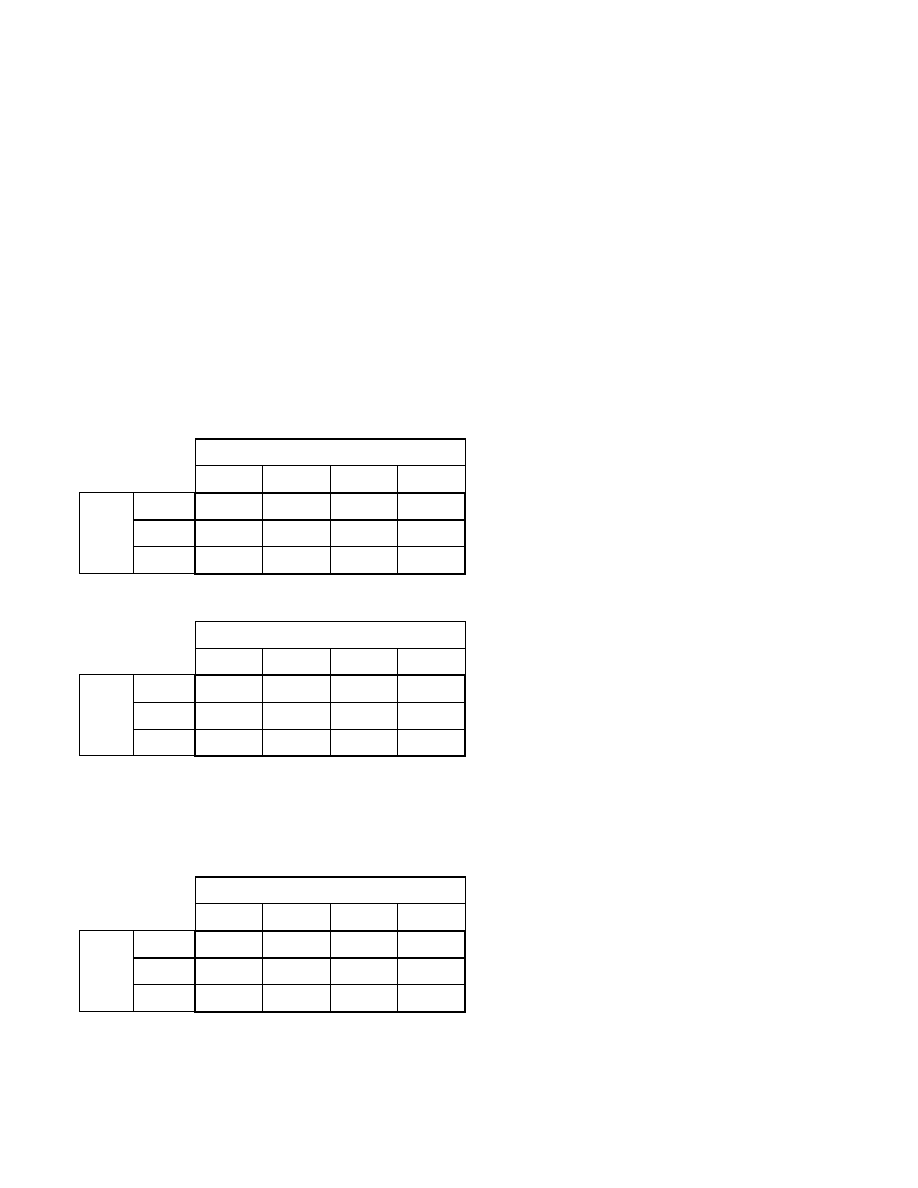
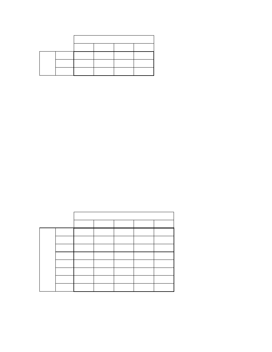
Here is an illustration of how list data are calculated using contributions from two RIV parameters, R1 and

R2. The data list for parameter R1 is:

Riverbed Riverbed

River Conductance Bottom

Layer Row Column Stage Multiplier Elevation

1 4 5 4.5 150 4.0

1 5 6 4.8 180 4.3

1 5 7 5.0 200 4.5

1 6 7 5.1 250 4.6

The data list for parameter R2 is:

Riverbed Riverbed

River Conductance Bottom

Layer Row Column Stage Multiplier Elevation

1 10 22 8.9 500 8.0

1 11 21 9.5 600 8.5

1 11 20 10.2 700 9.0

If R1 = 10, and R2 = 20, the resulting list data for the river is:

Riverbed

River Riverbed Bottom

Layer Row Column Stage Conductance Elevation

1 4 5 4.5 1500 4.0

1 5 6 4.8 1800 4.3

1 5 7 5.0 2000 4.5

1 6 7 5.1 2500 4.6

1 10 22 8.9 10000 8.0

1 11 21 9.5 12000 8.5

1 11 20 10.2 14000 9.0

Parameters for Layer Data

Each package that incorporates layer data may have any number of types of data to be defined. The input

instructions for a package indicate which data types can be defined using parameters. Each data type is given a
specific name that must be included as part of the input data that defines a parameter of that type. For example, in
the Layer-Property Flow Package, there are six types of layer data, such as horizontal hydraulic conductivity and
specific storage, that can be defined using parameters, and one, called WETDRY, that cannot. The parameter type
for horizontal hydraulic conductivity is HK, and the parameter type for specific storage is SS.

Ground-Water

Flow

Process

For layer data, parameter multipliers are defined using multiplier arrays. “Array” is programming

terminology for a variable that contains many values. In this case, each multiplier array contains values for every
cell in a layer, and the values can be individually referenced using a row and column index. There can be a
different multiplier array for every layer to which the parameter applies, and these are identified when the
parameter is defined. Thus, the multiplier for cell (i,j,k) is the (i,j) value of the multiplier array that is specified for
layer “k.”

To allow only some of the cells of a layer to be associated with a layer parameter, a capability called zonation

is used. Like multiplier arrays, each zone array is named and contains values for every cell in a layer. Values in a
zone array are integers. There can be a different zone array for every layer to which the parameter applies. When a
parameter is defined, the zone array and one or more zone values are specified. The parameter applies to cells at
which the value of the zone array matches any one of the specified zone values; that is, the data value at a cell is
the product of the multiplier array at the cell and the parameter value only if the value of the zone array matches
one of the zone values specified for the parameter.

Multiplier and zone arrays are defined as part of input to the Global Process. These arrays are read by the

array utility modules the same way as layer data for a single layer are read.

As an example of how layer data are calculated from parameters, consider the following multiplier and zone

arrays for a layer that has 3 rows and 4 columns.

Multiplier array:

Column

1 2 3 4

1 200. 30. 350. 400.

2 200. 30. 60. 400.

Row

3 15. 30. 60. 425.

Zone array:

Column

1 2 3 4

1 1 3 1 1

2 1 2 3 4

Row

3 3 3 3 5

If parameter P1 applies to values where the zone array is 2 or 3 and parameter P2 applies to values where the

zone array is 1, 4, or 5; then the following input values would be calculated.

Column

1 2 3 4

1 200

P2 30

P1 350

P2 400

2 200

P2 30

P1 60

P1 400

Row

3 15

P1 30

P1 60

P1 425

MODFLOW-2000—User Guide to Modularization Concepts and the

Ground-Water Flow Process

If P1=50 and P2 =80, the final result is:

Column

1 2 3 4

1 16000 1500 28000 32000

2 16000 1500 3000 32000

Row

3 750

1500

3000

34000

As already mentioned, a single layer parameter can specify data for multiple layers. For each layer that is

included in a parameter, there can be a different multiplier and zone array. The above procedure is applied to
calculate the data values for the cells in each layer.

As is shown in the example, the use of a multiplier array allows layer data that is determined by one

parameter to be different at each cell. Further, the relative values of the parameter-based layer data are the same as
the relative values of the multipliers regardless of the value of the parameter. Consider parameter P1 in the
example above. The multiplier for each successive column from left to right is twice the value of the previous
column. Thus, the resulting data values that are based on P1 also differ by a factor of 2 from left to right.

Case 2: Additive Parameters Are Used to Determine a Cell Data Value

In the above discussion, it is assumed that the data value for a cell is determined by a single parameter. It is

possible, however, for the value at a cell to be determined by more than one parameter. If two or more parameters
of the same type include the same cell, the final data value equals the sum of the contributions from all of the
parameters, where the contribution from each parameter is calculated as described above. When two or more
parameters are used to define the value for cells, the parameters are said to be additive.

As an example of using two parameters to determine the data values for the same cells, assume that it is

desired to have the distribution of horizontal hydraulic conductivity, which is layer data, vary linearly from 10 to
100 from the left side to the right side of a layer. This can be done using two additive parameters, P1 and P2, that
both apply to all cells in the layer. For a layer consisting of 8 rows and 5 columns, the multiplier array for P1 is:

Column

1 2 3 4 5

1 1.0 0.75 0.50 0.25 0.0

2 1.0 0.75 0.50 0.25 0.0

3 1.0 0.75 0.50 0.25 0.0

4 1.0 0.75 0.50 0.25 0.0

5 1.0 0.75 0.50 0.25 0.0

6 1.0 0.75 0.50 0.25 0.0

7 1.0 0.75 0.50 0.25 0.0

Row

8 1.0 0.75 0.50 0.25 0.0

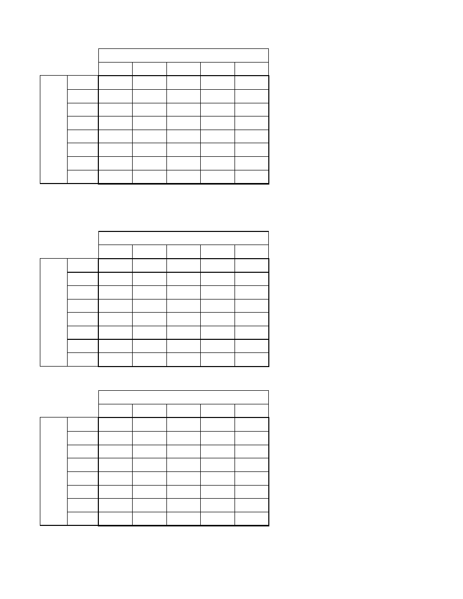
Ground-Water

Flow

Process

The multiplier array for P2 is:

Column

1 2 3 4 5

1 0.0 0.25 0.50 0.75 1.0

2 0.0 0.25 0.50 0.75 1.0

3 0.0 0.25 0.50 0.75 1.0

4 0.0 0.25 0.50 0.75 1.0

5 0.0 0.25 0.50 0.75 1.0

6 0.0 0.25 0.50 0.75 1.0

7 0.0 0.25 0.50 0.75 1.0

Row

8 0.0 0.25 0.50 0.75 1.0

If P1 = 10., and P2=100., the contributions from both parameters will be added as follows:

The multiplier array for P2 is:

Column

1 2 3 4 5

10+0 7.5+25 5+50 2.5+75 0+100

Row

10+0 7.5+25 5+50 2.5+75 0+100

The final result is the desired values:

Column

1 2 3 4 5

1 10.

32.5 55 77.5

100.

2 10.

32.5 55 77.5

100.

3 10.

32.5 55 77.5

100.

4 10.

32.5 55 77.5

100.

5 10.

32.5 55 77.5

100.

6 10.

32.5 55 77.5

100.

7 10.

32.5 55 77.5

100.

Row

8 10.

32.5 55 77.5

100.

MODFLOW-2000—User Guide to Modularization Concepts and the

Ground-Water Flow Process

This same distribution could be created in other ways. For example, it could be created without parameters

by simply reading the final data values as input data. It could also be generated using a single parameter by having
the multiplier vary linearly from 1.0 on the left and 10.0 on the right and having a parameter value be 10.0. There
would be an advantage of using two parameters, however, if there were a need to try many distributions that have
a linear variation from left to right. The two-parameter approach would allow any such linear distribution to be
created by simply changing the two parameter values.

Additive parameters can also be used for list data. Consider another hypothetical situation in which the River

Package is being used. In this situation the riverbed sediments are coarse grained at the head of the river and fine
grained at the mouth. The resulting riverbed conductance along the first three cells representing the river is
assumed to be a constant indicative of the coarse-grained sediments, and the conductance in the last three cells is
assumed to be a constant indicative of the fine-grained sediments. In the middle region of the river, which crosses
five model cells, it is assumed that the two materials are mixed in such a manner that the riverbed conductance
varies linearly from the coarse-grained value to the fine-grained value. This riverbed conductance distribution can
be represented by two additive parameters—one for the coarse-grained material and one for the fine-grained
material. The following is an example of a data set for this situation in which P1 represents the riverbed
conductance of the coarse-grained material and P2 represents the riverbed conductance of the fine-grained
material. The data list for parameter P1 is:

Riverbed Riverbed

River Conductance Bottom

Layer Row Column Stage Multiplier Elevation

1 7 9 7.5 1.0 7.0

1 8 9 6.8 1.0 6.3

1 9 9 5.9 1.0 5.4

1 10 9 5.1 .83 4.6

1 11 9 4.5 .67 4.0

1 12 9 3.8 .50 3.3

1 13 9 3.2 .33 2.7

1 14 9 2.5 .17 2.0

The data list for parameter P2 is:

Riverbed Riverbed

River Conductance Bottom

Layer Row Column Stage Multiplier Elevation

1 10 9 5.1 .17 4.6

1 11 9 4.5 .33 4.0

1 12 9 3.8 .50 3.3

1 13 9 3.2 .67 2.7

1 14 9 2.5 .83 2.0

1 15 9 2.1 1.0 1.6

1 16 9 1.8 1.0 1.3

1 17 9 1.5 1.0 1.0

Ground-Water

Flow

Process

Parameters P1 and P2 both include the five cells where the two riverbed materials are assumed to intermix,

so the riverbed conductance for those cells will be the sum of the components from both parameters. For example,
the river reach at cell (1, 12, 9) is in the middle of the transition region, and the conductance multipliers are both
0.5 so that the riverbed conductance will be the sum of half of P1 and half of P2.

In addition to the above examples of linear interpolation, additive parameters can be used to generate data

using many point-based interpolation techniques, such as distance weighting and kriging. While the regression
part of the pilot-point method (RamaRao and others, 1995) could be performed by MODFLOW-2000, the
selection of pilot points and redefinition of multiplication arrays for the kriging would need to be done externally.

Packages Included in this Report

This section very briefly describes the current versions of the 14 previously existing packages and one new

package that are included in the initial release of MODFLOW-2000 and discussed in this work. As has occurred
with previous versions of MODFLOW, other packages and their documentation may be added to U.S. Geological
Survey distributions of MODFLOW-2000. The 15 packages discussed in this document include

•

the 10 documented in McDonald and Harbaugh (1988),

•

the more recent solvers PCG2 (Hill, 1990) and DE4 (Harbaugh, 1995),

•

the Hydraulic Flow Barrier (HFB) Package (Hsieh and Freckleton, 1993),

•

the Time-Variant Specified Head Package (CHD; Leake and Prudic, 1991), and

•

the new Layer Property Flow Package (LPF).

The new Layer-Property Flow Package is completely documented in this report.

Previously Existing Packages

Basic (BAS) Package

The input requirements for the BAS Package data file in MODFLOW-2000 have been modified compared to

the MODFLOW-96 version (Harbaugh and McDonald, 1996a) to remove the parts that have been incorporated
into the Global Process discretization file. This includes the number of layers, rows, and columns in the grid and
the number and length of stress periods. Variables IAPART and ISTRT have also been eliminated from the BAS
input file. They were used to conserve memory, but the need to conserve memory on modern computers is not as
great as it used to be when MODFLOW was first developed. The elimination of ISTRT has an impact on default
output control—drawdown will no longer be printed for default output control, and an output control input file
will be needed to obtain drawdowns. All these changes make it necessary to modify an existing MODFLOW-96
BAS file in order to work with MODFLOW-2000. The remaining parts of the input file are the variables
HNOFLW, STRT (initial head), and IBOUND. The translation program described below will generate a
MODFLOW-2000 BAS file from a MODFLOW-96 BAS file.

The file type for the BAS Package input file in the Name File is BAS6. If a MODFLOW-96 Name File,

which would specify a file type of BAS for the BAS input file, is used, MODFLOW-2000 will stop the simulation
and print an error message indicating that the file type is illegal. This avoids the input errors that would occur if
the MODFLOW-2000 version of BAS were to read a MODFLOW-96 BAS input file.

When the Parameter-Estimation Process is used, the Ground-Water Flow BAS input file is rewound each

time the Ground-Water Flow Process is restarted so that the input data will be the same each time. For this reason,
the BAS Package writes its output to the LIST file, which is also rewound each time the Ground-Water Flow
Process is restarted if there is a GLOBAL file. The LIST file will therefore contain output from the BAS Package
for the last execution of the Ground-Water Flow Process.

The Output Control Option of the BAS Package has been modified to allow the boundary flag (variable

IBOUND) for every cell to be written into a disk file at the end of any time step. This is useful in simulations in
which cells switch between wet and dry, thus changing the value of IBOUND.

MODFLOW-2000—User Guide to Modularization Concepts and the

Ground-Water Flow Process

Block-Centered Flow (BCF) Package

The BCF Package functions internally exactly as in MODFLOW-96, which means that it includes the

original functionality (McDonald and Harbaugh, 1988, ch. 5), the capability to convert dry cells to wet
(McDonald and others, 1992), and alternate methods for calculating interblock transmissivity (Goode and Appel,
1992). The MODFLOW-2000 version has been modified, however, so that it no longer reads any discretization
data. Instead, it uses the horizontal grid spacing (DELR and DELC), layer elevation (TOP and BOT variables in
MODFLOW-96), and transient/steady-state data included in the Global Process discretization file. Therefore, an
existing MODFLOW-96 BCF file must be modified to work with MODFLOW-2000. The translation program
(MF96TO2K) described below will generate a MODFLOW-2000 BCF file from a MODFLOW-96 BCF file.

The layer elevations defined in the discretization file are not always used by the BCF Package. Specifically,

transmissivity and storage coefficient for confined layers, and the vertical leakance (VCONT) for all layers, are
directly read by the BCF Package, and these values incorporate layer thickness. Thus, the global elevation data
will not have any impact on BCF calculations in which these input data are used. Further, the BCF Package will
not make use of the information in the discretization file that defines confining beds that are simulated using the
Quasi-3D Approach because this method is handled in BCF by incorporating the effect of the confining bed in the
user-specified VCONT values (McDonald and Harbaugh, 1988, p. 5-16). When the BCF Package is active, the
global elevation data from the discretization file are used only for the head-dependent formulations: saturated
thickness calculation for water-table and convertible layers, storage conversion for convertible layers, and vertical
flow limitation that occurs when the hydraulic head in a layer falls beneath the bottom of the layer above.

The parameter method of data input has not been incorporated into the BCF Package. The new Layer-

Property Flow Package, which can substitute for BCF, incorporates parameters.

The file type for the BCF Package input file in the name file is BCF6. If a MODFLOW-96 name file, which

would specify a file type of BCF for the BCF input file, is used; MODFLOW-2000 will stop the simulation
because of an illegal file type. This avoids the input errors that would occur if the MODFLOW-2000 version of
BCF were to read a MODFLOW-96 BCF input file. The BCF Package writes all of its output to the LIST file.

Horizontal Flow Barrier (HFB) package

The capability to simulate thin, vertical, and low-permeability geologic features was added to MODFLOW

with the introduction of the Horizontal Flow Barrier Package (Hsieh and Freckleton, 1993). As originally written,
this package was designed to work with the Block Centered Flow Package. The Horizontal Flow Barrier (HFB)
Package has been modified to accommodate the use of parameters and to work with either the Block-Centered
Flow Package or the new Layer-Property Flow Package.

The HFB package theory and methodology are unchanged from the original implementation. As described in

Hsieh and Freckleton (1993), HFB performs its function by adjusting hydraulic conductance between adjacent
cells in a layer. The only changes made for MODFLOW-2000 are in the input requirements and in the support for
parameters and parameter estimation. Note that in the terminology of the HFB Package, a barrier is situated on the
boundary between two adjacent finite-difference cells in the same layer. Parameters defined in the HFB Package
control the hydraulic characteristic of one or more horizontal-flow barriers.

The original version of the HFB Package required the input of the hydraulic characteristic either as barrier

transmissivity divided by the width of the horizontal-flow barrier (for layer types 0 and 2 in BCF) or as barrier
hydraulic conductivity divided by the width of the horizontal-flow barrier (for layer types 1 and 3 in BCF). In the
current HFB Package, the hydraulic characteristic is always the barrier hydraulic conductivity divided by the
width of the barrier, regardless of the layer type or flow package (BCF or LPF) used; thus, layer thickness is
always used in calculating the contribution to the conductance terms. The HFB Package uses cell elevations
specified in the discretization file to calculate cell thickness. Cell thickness is head dependent for layer types 1
and 3 in the BCF Package and for convertible layers in the Layer-Property Flow Package.

The file type for the HFB Package input file in the Name File is HFB6. If a Name File lists a file of type

HFB, MODFLOW-2000 will stop the simulation with an error message indicating that an illegal file type was
specified. If this error message is encountered, the user should ensure that the file associated with this file type is
compatible with the current version of the HFB Package and change the file type to HFB6. Input errors would
occur if the MODFLOW-2000 version of HFB were to read an input file prepared for the original version of HFB.

Ground-Water

Flow

Process

Source-Term Packages

These packages are divided according to whether they are head dependent or head independent. They have

all been modified to incorporate parameters. Other than the addition of parameters, these packages function the
same as in MODFLOW-96. Input files for MODFLOW-96 will still work in MODFLOW-2000. All of the output
is written to the LIST file.

Head-Dependent Packages

RIV—The riverbed conductance can be defined using parameters.

DRN—The drain conductance can be defined using parameters.

GHB—The boundary conductance can be defined using parameters.

EVT—The maximum evapotranspiration flux can be defined using parameters.

McDonald and Harbaugh (1988) document the concepts of the RIV, DRN, GHB, and EVT Packages.

Head-Independent Packages

WEL—The well recharge rate (negative sign indicates discharge) can be defined using parameters.

RCH—The Recharge flux can be defined using parameters.

McDonald and Harbaugh (1988) document the concepts of both of these packages.

Time-Variant Specified-Head Package

MODFLOW-2000 contains the Time-Variant Specified-Head (CHD) Package (Leake and Prudic, 1991), and

this has been modified to allow parameters to define the specified head. Input files for MODFLOW-96 will still
work in MODFLOW-2000. All of the output is written to the LIST file.

Solver Packages

Four solvers are included in MODFLOW-2000:

SIP—strongly implicit procedure (McDonald and Harbaugh, 1988),

SOR—slice successive overrelaxation (McDonald and Harbaugh, 1988),

PCG—preconditioned Conjugate Gradient (Hill, 1990), and

DE4—direct solution based on alternating diagonal ordering (Harbaugh, 1995).

There is no fundamental change to the solvers in MODFLOW-2000. From the perspective of the solvers, the

information that defines the simultaneous equations that must be solved at each cell is exactly the same as in
earlier versions of MODFLOW. The solvers were modified superficially to allow them to be used by the
Sensitivity Process. The user-specified input data to control the solvers is unchanged from that used in
MODFLOW-96, except for a minor change for the PCG Package. A new option has been added to the PCG
Package, which outputs solver convergence information only if the solver fails to meet closure criteria. Otherwise,
no convergence information is written. Input files for MODFLOW-96 will still work in MODFLOW-2000.
Package identification and information that confirms what was read from the solver package input file is written
to the GLOBAL file. Convergence information is written to the LIST file.

MODFLOW-2000—User Guide to Modularization Concepts and the

Ground-Water Flow Process

New Package: Layer-Property Flow Package

Introduction

The Layer-Property Flow (LPF) Package is an internal flow package, so, as previously mentioned, it

calculates the CV, CR, and CC conductance coefficients and the parts of HCOF and RHS (equation 3) dealing
with ground-water storage. The BCF Package also performs this same function, and accordingly, LPF should be
viewed as an alternative to the BCF Package. That is, both packages should not be used simultaneously. The
following documentation of the LPF Package highlights the similarities and differences between the two
packages.

When calculating conductance coefficients, it is assumed in the LPF Package that a node is located at the

center of each model cell. The same assumption is also used in the BCF Package, and accordingly, the BCF and
LPF Packages are conceptually quite similar. The differences are primarily in the input data that the user
specifies. All the input data that define hydraulic properties are independent of cell dimensions in LPF, whereas
some of the input data for the BCF Package incorporate cell dimensions. For example, in some situations, the user
specifies transmissivity as input data for the BCF Package, but LPF never reads transmissivity. Instead, LPF
always reads hydraulic conductivity (either directly or using parameters) and calculates transmissivity by using
cell thickness that is determined from the global elevation data. Similarly, vertical leakance (hydraulic
conductivity divided by distance between nodes) is directly read by the BCF Package whereas the LPF Package
calculates leakance from vertical hydraulic conductivity and distance between nodes, which is calculated from the
global elevation data.

Basic Hydraulic Conductance Equations

The concept of hydraulic conductance (shortened to conductance to save space in this report) is defined in

McDonald and Harbaugh (1988, chs. 2 and 5). It is reviewed here, including the calculation of equivalent
conductance for elements arranged in series. Conductance is a combination of several parameters used in Darcy’s
law. Darcy’s law defines one-dimensional flow in a prism of porous material (fig. 3) as

)

KA(h

−

(4)

where

Q is the volumetric flow (L

-1

);

K is the hydraulic conductivity of the material in the direction of flow (LT

-1

);

A is the cross-sectional area perpendicular to the flow (L

);

-h

is the head difference across the prism parallel to flow (L); and

L is the length of the prism parallel to the flow path (L).

Conductance, C, is defined as

(5)

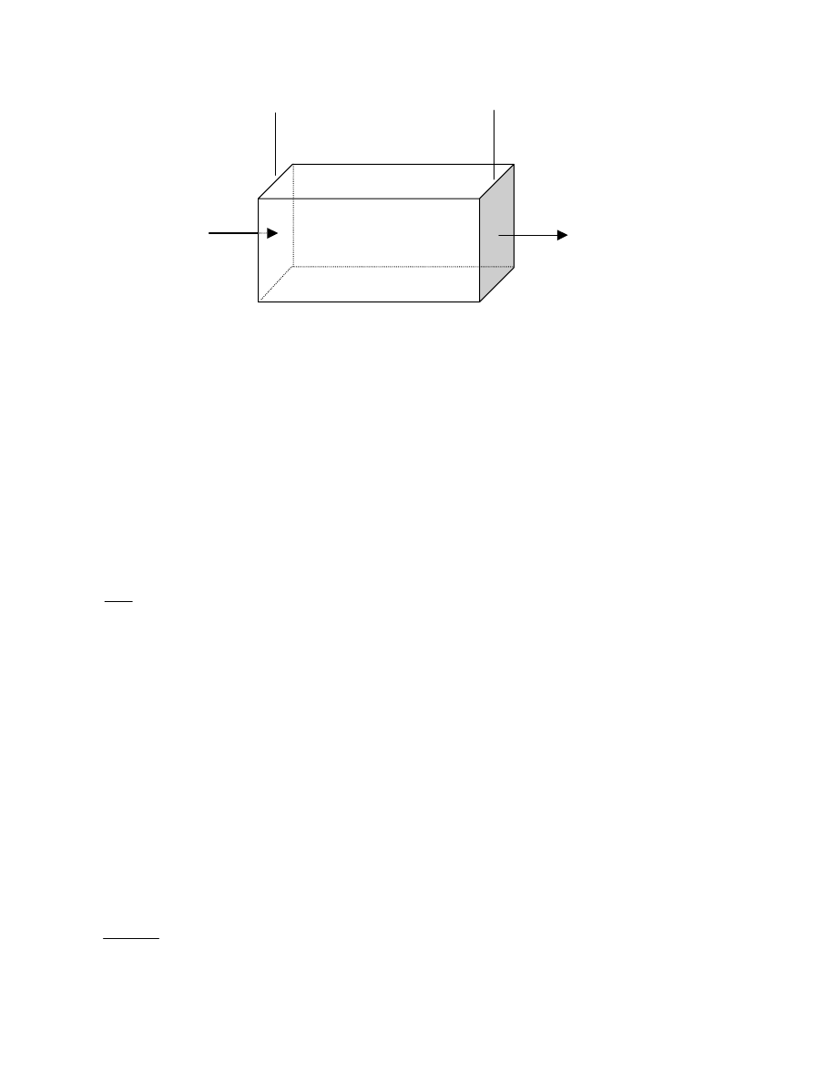
Ground-Water

Flow

Process

Figure 3.--Prism of porous material illustrating Darcy’s law.

Therefore, Darcy’s law can be written as

)

C(h

(6)

Another form of the conductance definition for horizontal flow in a prism is

(7)

where

T is transmissivity (K times thickness of the prism) in the direction of flow (L

-1

); and

W is the width if the prism (L).

Conductance is defined for a particular prism of material and for a particular direction of flow. In an

anisotropic medium that is characterized by three principal directions of hydraulic conductivity, the
conductances of a prism in these three principal directions will generally differ.

If a prism of porous material consists of two or more subprisms in series (aligned sequentially in the

direction of flow) as shown in figure 4, and the conductance of each subprism is known, a conductance
representing the entire prism can be calculated. The equivalent conductance for the entire prism is the rate of
flow in the prism divided by the head change across the prism.

−

(8)

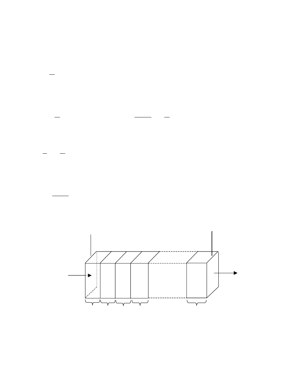
MODFLOW-2000—User Guide to Modularization Concepts and the

Ground-Water Flow Process

Assuming continuity of head across each section gives the identity

−

∑

(9)

Substituting for head change across each section using Darcy’s law (equation 6) gives

−

∑

(10)

Because flow is one dimensional, and we are assuming no accumulation or depletion in storage, all q

are equal to

the total flow Q; therefore,

−

∑

and

∑

−

(11)

By comparing equation 11 with equation 8, it can be seen that

∑

(12)

Thus for a set of conductances arranged in series, the inverse of the equivalent conductance equals the sum of the
inverses of the individual conductances. When there are only two sections, the equivalent conductance reduces to

(13)

Figure 4.-- Calculation of conductance through several prisms in series.

∆

Ground-Water

Flow

Process

Horizontal Conductance

The finite-difference equations in MODFLOW use equivalent conductances between nodes of adjacent

cells—that is, “branch conductances”—rather than conductances defined within individual cells. The horizontal
conductance terms, CR and CC of equation 2, are calculated between adjacent horizontal nodes. CR terms are
oriented along rows and thus specify conductance between two nodes in the same row. Similarly, CC terms
specify conductance between two nodes in the same column. (Remember that the "1/2" subscript denotes
conductance between nodes, as opposed to conductance within a cell. For example, CR

i,j+1/2,k

represents the

conductance between nodes i,j,k and i,j+1,k.)

The LPF Package reads data defining the horizontal hydraulic conductivity for individual cells and calculates

conductance between nodes. Three methods of calculating these conductances are supported. The methods differ
in the assumptions about the way the ground-water system varies from cell to cell.

Constant Product of Hydraulic Conductivity and Thickness within a Cell

The first method is based on the assumption that hydraulic conductivity times thickness, that is,

transmissivity, is constant within a cell. There can, therefore, be a discrete change in transmissivity at the
boundary between any two cells. By use of this assumption and the previously mentioned assumption in LPF that
nodes are in the center of cells, the conductance between the nodes is the equivalent conductance of two half cells
in series. Figure 5 illustrates two cells along a row based on these assumptions. Substituting the conductance for
each half cell (equation 7) into equation 13 gives:

)DELR

(

DELC

)DELR

(

DELC

)DELR

(

DELC

)DELR

(

DELC

(14)

where

i,j,k

is transmissivity in the row direction at cell i,j,k (L

-1

);

DELR

is the grid width of column j (L); and

DELC

is the grid width of row i (L).

Figure 5.-- Calculation of conductance between nodes using transmissivities

and dimensions of cells.

DELR

j+1

i,j+1/2,k

i,j+1,k

DELC

i,j,k

i,j+1,k

i,j,k

MODFLOW-2000—User Guide to Modularization Concepts and the

Ground-Water Flow Process

Simplification of equation 14 gives the final equation:

DELR

DELC

(15)

The same process can be applied to the calculation of CC

i+1/2,j,k

giving:

DELC

DELR

(16)

where

i,j,k

is the transmissivity in the column direction at cell i,j,k (L

-1

Equations 15 and 16 are used unless the transmissivity of both cells is zero, in which case the conductance
between the nodes is set equal to zero without invoking the equations.

Transmissivity is calculated as:

THICK

(17A)

HANI

THICK

(17B)

where

i,j,k

is the hydraulic conductivity of cell i,j,k in the row direction (LT

-1

HANI

i,j,k

is the ratio of hydraulic conductivity along columns to the hydraulic conductivity along rows

(dimensionless), and

THICK

i,j,k

is the saturated thickness of cell i,j,k (L).

i,j,k

and HANI

i,j,k

are specified as input data. Values of THICK

i,j,k

are calculated using cell elevations in the

discretization file. The calculation of thickness depends on whether the layer is designated as confined or
convertible. This designation is made through the layer type-flag, LAYTYP, which is discussed in the Data
Requirements Section. In a model layer that is designated as confined, the thickness is the cell thickness:

THICK

i,j,k

= (TOP

i,j,k

-BOT

i,j,k

)

(18)

where

TOP

i,j,k

is the elevation of the top of cell i,j,k (L); and

BOT

i,j,k

is the elevation of the bottom of cell i,j,k (L).

TOP and BOT are determined from data in the discretization file.

Ground-Water

Flow

Process

If a layer is designated as convertible, then saturated thickness is calculated throughout the simulation based

upon the head (HNEW

i,j,k

if HNEW

i,j,k

≥

TOP

i,j,k

then THICK

i,j,k

= (TOP

i,j,k

- BOT

i,j,k

) ;

(19A)

if TOP

i,j,k

> HNEW

i,j,k

> BOT

i,j,k

then THICK

i,j,k

= (HNEW

i,j,k

- BOT

i,j,k

) ;

(19B)

if HNEW

i,j,k

≤

BOT

i,j,k

then THICK

i,j,k

= 0 .

(19C)

At the start of every iteration for solving the flow equation, cell transmissivity values (TR and TC) are
recalculated as the product of hydraulic conductivity and saturated thickness (equation 14); then conductance is
recalculated using equations 15 and 16. If head drops below the aquifer bottom (equation 19C), the cell is
considered to be fully dewatered, and is set to no flow by changing IBOUND

i,j,k

to 0. The model also has

provision for the resaturation of fully dewatered cells, which is described in another section of this report.

Note that unlike the LPF Package, the BCF Package has a special layer type for a water table in layer 1. This

BCF layer type always uses equation 19B for calculating saturated thickness. In LPF, the convertible formulation
should be used if layer 1 represents a water table. Also, the elevation of the top of layer 1, which is specified in
the discretization file, should be higher than the water level will reach at any time in the simulation. This will
result in the use of equation 19B for calculating saturated thickness. It is the user’s responsibility in this situation
to check to see that the simulated water level has not exceeded the top elevation, which would trigger the use of
equation 19C for calculating saturated thickness. A logical approach for specifying the top elevation for a layer-1
water table is to set it equal to land-surface elevation. That is, in most situations, it is not expected that the water
table will exceed land-surface elevation.

The above approach for calculating interblock conductance is called the “harmonic mean” method. The

reason for this name can be see by manipulating equation 15 into the following:

DELR

(½)

DELR

(½)

DELC

DELR

(½)

DELR

(½)

DELR

(½)

DELR

(½)













(20)

The term in parentheses is the distance weighted harmonic mean of transmissivity of the two half cells, which by
comparison with equation 7, can be seen to be the equivalent transmissivity between nodes i,j,k and i,j+1,k.

Alternative Approaches for Calculating Horizontal Branch Conductances

Goode and Appel (1992) discuss three alternative approaches for calculating the horizontal branch

conductances. These alternative approaches are each based on different assumptions about the flow system:
(1) transmissivity varies linearly between nodes, (2) flat, homogeneous aquifer with a water table, (3) flat aquifer
with a water table in which hydraulic conductivity varies linearly between nodes. For each approach, a
formulation of interblock transmissivity is developed. The interblock conductance is then computed as the
interblock transmissivity times cell width divided by distance between nodes according to equation 7.

When transmissivity varies linearly between nodes, the interblock transmissivity derived by Goode and

Appel (1992) is:

(

)

−

(21)

MODFLOW-2000—User Guide to Modularization Concepts and the

Ground-Water Flow Process

where subscripts 2 and 1 indicate any two adjacent cells along a row or column. This is called the “logarithmic
mean” interblock transmissivity method. This formulation will produce exact solutions for steady-state one-
dimensional flow if flow is uniform and aligned with the direction of changing transmissivity. To save numerical
effort, this function is approximated by

when 0.995

≤

1.005 .

For an unconfined homogeneous aquifer with a flat bottom, the interblock transmissivity derived by Goode

and Appel (1992) is:

(22)

This is called the “arithmetic mean” interblock transmissivity method. This formulation will produce exact
solutions for uniform, steady-state, one-dimensional flow.

For an unconfined aquifer with a flat bottom and with hydraulic conductivity varying linearly between nodes,

Goode and Appel derive the interblock transmissivity as:

(

)









−













THICK

(23)

This is called the “arithmetic mean thickness and logarithmic-mean hydraulic conductivity” method. This
formulation produces exact solutions for uniform, steady-state, one-dimensional flow when the hydraulic
conductivity varies in the direction of flow. To save numerical effort, the hydraulic conductivity part of this

function is approximated by

when 0.995

≤

1.005.

Because equation 23 reduces to equation 22 when the aquifer is homogeneous, equation 22 is not separately

included in the LPF Package. That is, only equations 21 and 23 are included in the LPF Package along with the
harmonic mean method.

Vertical Conductance

Vertical conductance is calculated assuming that nodes are in the center of cells and that there can be discrete

changes in vertical hydraulic conductivity at layer boundaries. Figure 6 illustrates this situation for two cells in
layers k and k+1. Under these assumptions, the vertical conductance between two nodes will be the equivalent
conductance of two half cells in series. Substituting the conductance for each half cell from equation 5 into
equation 12 gives

THICK

(½)

DELC

DELR

THICK

(½)

DELC

DELR

(24)

where

i,j,k

is vertical hydraulic conductivity of cell i,j,k and

THICK

i,j,k

is the saturated thickness of cell i,j,k as defined by equation 18 for confined cells and

equation 16 for convertible cells.

Ground-Water

Flow

Process

Figure 6.-- Calculation of vertical conductance between two nodes.

THICK

i,j,k

THICK

i,j,k+1

DELR

i,j,k+1/2

i,j,k

DELC

i,j,k

i,j,k+1

Simplification of equation 24 gives

THICK

(½)

THICK

(½)

DELC

DELR

(25)

Figure 7 shows a second situation, in which cells i,j,k and i,j,k+1 are separated by a semiconfining unit. If the

assumptions are made that the semiconfining unit makes no measurable contribution to the horizontal
conductance or the storage capacity of either model layer, then the only effect of the confining bed is to restrict
vertical flow between the model cells. Under these assumptions, the impact of the semiconfining unit can be
simulated without using a separate layer in the finite-difference grid. This is done by including the semiconfining
unit in the calculation of vertical conductance between the nodes. As mentioned previously, this is commonly
referred to as the "Quasi-Three-Dimensional" (QUASI-3D) Approach (McDonald and Harbaugh, 1988, p. 5-18).

MODFLOW-2000—User Guide to Modularization Concepts and the

Ground-Water Flow Process

Figure 7.-- Calculation of vertical conductance between two nodes with a

semiconfining unit between.

THICK

i,j,k+1

THICK

i,j,k

DELR

i,j,k+1/2

i,j,k

DELC

i,j,k

i,j,k+1

THICK

CBVK

i,j,k

In the Quasi-3D Approach, three intervals must be represented in the summation of conductance between the

nodes—the lower half of the upper aquifer, the semiconfining unit, and the upper half of the lower aquifer.
Equation 12 can be used to write an expression for the inverse of vertical conductance:

THICK

(½)

DELC

DELR

THICK

VKCB

DELC

DELR

THICK

(½)

DELC

DELR

(26)

where

VKCB

i,j,k

is the hydraulic conductivity of the semiconfining unit between cell i,j,k and i,j,k+1, and

THICK

is the thickness of the semiconfining unit.

THICK

is determined from information in the discretization file, and VKCB

i,j,k

is input data for the LPF

Package.

Ground-Water

Flow

Process

Simplification of equation 26 produces

THICK

½)

(

VKCB

THICK

½)

(

DELC

DELR

(27)

Vertical Flow Calculation Under Dewatered Conditions

This section describes a modification to the vertical flow calculation that is applied when a cell in a

convertible layer is unconfined (head is below its top elevation), while the cell immediately above is fully or
partially saturated. (Convertible layers are specified through the layer type-flag, LAYTYP, which is described in
the Data Requirements Section.) The vertical flow correction is applied for every solver iteration.

From equation 2, the term that represents the flow into cell i,j,k through its lower face, which will be called

i,j,k+1/2

, is

(

)

−

(28)

where the m superscript that indicates the time step has been removed. Following the convention of MODFLOW,
a positive value of q

i,j,k+1/2

indicates flow into cell i,j,k, and a negative value indicates flow out of the cell.

Equations 2 and 28 are based on the assumption that cells i,j,k and i,j,k+1 are fully saturated—that is, that the
hydraulic head in each cell stands higher than the elevation of the top of the cell.

There are, however, situations in which a part of a confined aquifer may become unsaturated—for example,

when drawdown due to pumpage causes water levels to fall, at least locally, below the top of an aquifer. This
condition is most likely to occur when an aquifer is overlain by a lower conductivity unit. In terms of simulation,
this condition is shown in figure 8. Cells in two model layers are represented. The upper cell (i,j,k) has lower
hydraulic conductivity than the underlying cell (i,j,k+1), which represents an aquifer. Pumping from the lower
layer has lowered the water level in cell i,j,k+1 below the elevation of the top of the cell; however, cell i,j,k
remains fully saturated. Thus, cell i,j,k+1 is effectively unconfined even though the cell above is saturated.

Consider the calculation of flow between nodes in the upper and lower cells. In the upper cell, head is simply

whatever head is at that cell—h

i,j,k

. Just below the upper cell, however, unsaturated conditions prevail, so that the

pressure sensed on the lower surface of the confining unit is atmospheric—taken as zero in the model
formulation. Thus the head at the bottom of the upper cell is simply the elevation at that point—that is, the
elevation of the top of the lower cell. If this elevation is designated TOP

i,j,k+1

, then the actual flow through the

confining bed is obtained by substituting TOP

i,j,k+1

for h

i,j,k+1

in equation 28,

(

)

TOP

−

(29)

Thus, the flow will be downward, from cell i,j,k to cell i,j,k+1, but under this condition the flow will no

longer be dependent on the water level, h

i,j,k+1

, in the lower cell. The simplest approach to this problem in

formulating the equation for cell i,j,k would be to substitute the flow expression of equation 29 into equation 2, in
place of the expression given in equation 28. However, if we consider the matrix of coefficients of the entire
system of finite-difference equations, this direct substitution would render this matrix asymmetric, generating
problems in the solution process.

MODFLOW-2000—User Guide to Modularization Concepts and the

Ground-Water Flow Process

Figure 8.-- Situation in which a correction is required to limit the down-
ward flow into cell i,j,k+1, as a result of partial desaturation
of the cell.

i,j,k

representing
semiconfining unit

i,j,k

i,j,k+1

representing
aquifer unit

i,j,k+1

TOP

i,j,k+1

i,j,k

To avoid this condition, an alternative approach is used. The flow term of equation 28 is allowed to remain on

the left side of equation 2. The "actual" flow into cell i,j,k is given by equation 29, so a correction term, q

, can be

obtained by subtracting equation 29 from equation 28:

= (computed flow into cell i,j,k) - ("actual" flow into cell i,j,k)

(30)

= CV

i,j,k+1/2

i,j,k+1

– TOP

i,j,k+1

) .

This correction term, q

should be added to the right side of equation 2 to compensate for allowing the computed

flow to remain on the left side of equation 2. This again introduces a problem of matrix unsymmetry because q

contains the term h

i,j,k+1

. To circumvent this difficulty, q

is actually computed using the value of h

i,j,k+1

from the

preceding iteration, rather than that from the current iteration:

(

)

TOP

n
c

−

(31)

Ground-Water

Flow

Process

where

n
c

is the value of q

to be added to the right side of equation 2 in the nth iteration, and

−

is the value of h

i,j,k+1

from the preceding iteration, n-1.

As convergence is approached, the difference between

−

and

becomes progressively smaller, and the

approximation involved in equation 31 thus becomes more accurate. In the first iteration of each time step, the
initial trial value of h

i,j,k+1

is used in computing q

. In terms of equation 3, which is the form of the flow equation

that is directly implemented in MODFLOW,

n
c

is added to RHS

i,j,k

The process described above is used in formulating the equations for cell i,j,k when the underlying cell,

i,j,k+1, has "dewatered"—that is, when the water level in i,j,k+1 has declined below the top of the cell. A
correction must also be applied in formulating the equations for the dewatered cell itself. To compute this
correction, cell i,j,k is considered to be the dewatered cell, and we consider flow into i,j,k from the overlying cell,
i,j,k-1. For this case, the computed flow into cell i,j,k from above is

i,j,k-1/2

i,j,k-1

- h

i,j,k

) .

whereas the "actual" flow into the cell is

i,j,k-1/2

i,j,k-1

- TOP

i,j,k

) .

The difference, computed minus "actual" flow, is thus

′

= CV

i,j,k-½

(TOP

i,j,k

– h

i,j,k

) (32)

where q

′

is added to the right-hand side of equation 2. From a programming point of view, the most efficient way

to handle this correction is to add the term CV

i,j,k-1/2

to HCOF on the left side of equation 2, while adding the term

i,j,k-1/2

TOP

i,j,k

to the RHS term. However, this causes difficulties for some solution methods because it reduces

the dominance of the diagonal of the coefficient matrix of the finite-difference equations. So the same approach is
used as described previously for the vertical correction for the cell above the dewatered cell. That is, q

′

computed on the basis of the head from the previous iteration, and this correction is added to RHS of equation 3.

This conceptualization of limiting vertical flow is also valid when the unsaturated region in a lower layer is

caused by an overlying confining unit that is simulated using the Quasi-3D Approach. Although the confining unit
is not simulated as a separate model layer when using this approach, the impact of the confining unit is still
simulated through the vertical conductance calculation. The above vertical flow calculation correction is applied.
The value of TOP

i,j,k

is the bottom of the confining bed.

Note that when vertical leakage is limited, an argument could be made that the vertical conductance

calculation should also be modified. That is, the vertical conductance should not include any contribution from
the lower cell that is partially dewatered. However, this modification of vertical conductance has not been
incorporated into this version of the program.

In summary, whenever dewatering of a cell occurs below a cell that is not fully dewatered, two corrections

must be made—one in formulating equation 2 as it applies to the overlying cell, and one in formulating equation 2
as it applies to the dewatered cell itself. These two corrections are discussed separately above, in each case using
the designation i,j,k to represent the cell for which equation 2 is formulated. It is important to keep in mind,
however, that both corrections are applied in any dewatering event, and that the form of the corrections has been

MODFLOW-2000—User Guide to Modularization Concepts and the

Ground-Water Flow Process

developed to preserve the symmetry of the coefficient matrix of the finite-difference equations and its diagonal
dominance. This correction is applied as described for layers that are designated as convertible layers.

Conversion from Dry to Wet

When saturated thickness is 0 as defined by head being less than the bottom elevation of a cell

(equation 19C), it is clear that a variable-head (wet) cell should convert to dry. Unfortunately, there is not a
straight-forward way to know when a dry cell should convert to wet. McDonald and others (1992) describe an
approach for doing this and its application in the BCF Package of MODFLOW. The same approach is applied to
the LPF Package. The following is a brief overview of the approach. Readers should refer to McDonald and
others (1992) for additional details. In particular, that report describes detailed information about numerical
instabilities that can result from using this option, and several test problems are included.

A dry cell converts to wet based upon the head in an adjacent cell compared to a wetting threshold,

THRESH, for the cell. If the head at an adjacent cell equals or exceeds the threshold at the start of a solution
iteration, the dry cell is converted to wet. The only cells that can cause a dry cell to convert to wet are the four
cells that are immediately adjacent to the cell horizontally and the cell immediately below. There is also an option
to use only the cell below to determine that a dry cell becomes wet. The head below can be a better wetting
indicator than the head at horizontally adjacent cells when the head variations between adjacent horizontal cells
are larger than the vertical head variations, which is frequently the case.

A primary difficulty with this approach is that the value of THRESH must be determined by trial and error. If

THRESH is too low, a cell may be incorrectly converted to wet. That is, a cell may convert to wet and then
reconvert to dry in later solver iterations because the head does not stay above the bottom elevation. This cycle of
converting between wet and dry can repeat indefinitely, preventing the solver from converging. Larger values of
THRESH can avoid repeated conversion between wet and dry, but they increase the nonuniqueness of the solution
(McDonald and others, 1992, p. 8).

When a cell converts to wet, the initial estimate of head is established according to one of two equations:

i,j,k

= BOT

i,j,k

+ WETFCT(h

– BOT

i,j,k

)

(33A)

i,j,k

= BOT

i,j,k

+ WETFCT(THRESH

i,j,k

)

(33B)

where

WETFCT is a user-specified constant, generally between 0 and 1, and
h

is the head at the neighboring cell that causes cell i,j,k to convert to wet.

The user chooses the equation that works best for the problem being simulated. The initial estimate of head at a
cell that converts to wet is theoretically unimportant because the solver should calculate the correct value in
subsequent iterations. In practice, however, the initial estimate is often important for solver efficiency; that is, if a
poor choice is made, the solver convergence may be slower than optimum. A bad choice for initial head can also
cause the cell to oscillate between wet and dry.

Another user-specified option is the solver iteration interval for attempting to wet cells. For example, if the

interval is 4, cell wetting is attempted every 4 iterations. This can prevent the normal fluctuations in heads that
can occur in iterative solvers in the next few iterations after cells are converted to wet from inappropriately
triggering more cell wetting. All of these options are included to help make the solution process more stable.
Refer to McDonald and others (1992) for more information about solution instability and how to deal with it.

Storage Formulation

The LPF Package formulates storage terms for transient stress periods much as done for the BCF Package

(McDonald and Harbaugh, 1988, p. 5-24). LPF makes the same distinction between confined layers for which
storage terms remain constant throughout the simulation, and those in which the storage terms may "convert"

Ground-Water

Flow

Process

from a confined value to a water table value, or conversely, as the water level in a cell falls below or rises above
the top of the cell. In LPF, this distinction is made through the layer-type flag, LAYTYP, as described in the Data
Requirements Section.

For a confined layer, the storage formulation is based upon a direct application of the storage expression in

equation 2. This expression for the rate of accumulation of water into a single cell is:

(

)

THICK

DELC

DELR

ûW

û9

−

(34)

where

i,j,k

is the specific storage of the material in cell i,j,k (L

-1

);

THICK

i,j,k

is the cell thickness as defined by equation 18 (L);

is the head in cell i,j,k at the end of time step m (L);

−

is the head in cell i,j,k at the end of time step m-1 (L);

is the time at the end of time step m (T); and

m-1

is the time at the end of time step m-1 (T).

The notation SC1

i,j,k

is introduced where SC1

i,j,k

(DELR

DELC

THICK

i,j,k

). In this report the term

SC1

i,j,k

is termed the "storage capacity" or the "primary storage capacity" of cell i,j,k; the "primary" designation is

used to distinguish SC1

i,j,k

from a secondary storage capacity, which is used when storage term conversion is

invoked, as explained in the following section. By using the concept of storage capacity, equation 34 can be
rewritten as

SC1

ûW

û9

−

(35)

This expression is separated into two terms for inclusion into equation 3:

SC1

−

which is incorporated in the left side of equation 3 through the term HCOF

i,j,k

, and

SC1

−

which is included in the term RHS

i,j,k

on the right side of equation 3.

The input to the Layer-Property Flow Package requires specification of specific storage values for each cell

of the model if there are one or more transient stress periods. The specific storage values are read layer by layer;
and then they are multiplied by the cell areas and layer thickness to create storage capacity values, which are
stored in variable SC1.

Storage Term Conversion

The primary storage capacity described above, SC1

i,j,k

is adequate for simulations in which a cell is confined

throughout the course of a simulation; however, if the water level is below the top of a cell during a simulation,
then the cell is under a water-table condition, and a different storage formulation applies:

MODFLOW-2000—User Guide to Modularization Concepts and the

Ground-Water Flow Process

(

)

DELC

DELR

ûW

û9

−

(36)

where

SY is the specific yield (dimensionless).

A secondary storage capacity, SC2

i,j,k

, is used to represent specific yield multiplied by cell area, and

equation 36 can be written as

SC2

ûW

û9

−

(37)

During any one time step, there are four possible storage conditions for each cell:

The cell is confined for the entire time step,
The cell is unconfined for the entire time step,
The cell converts from confined to unconfined, and
The cell converts from unconfined to confined.

The following expression for rate of accumulation in storage in cell i,j,k is used to handle all four possibilities:

(

)

(

)

TOP

SCA

TOP

SCB

ûW

û9

−

(38)

where

TOP is the elevation of the top of the model cell,
SCA is the storage capacity in effect in cell i,j,k at the start of the time step; and
SCB is the "current" storage capacity—that is, the storage capacity in effect during the current iteration.

Equation 38 handles the four situations as follows: First, consider a case in which the head in cell i,j,k at the
beginning of time step m (

−

) is above the top of the cell (fig. 9). Because there is no free surface in the cell at

the start of the time step, the storage capacity at that time is taken as the confined storage capacity; that is, SCA is
set equal to SC1

i,j,k

. If, during a given iteration for time step m, the computed value of head for the end of the time

step (

) is found to be above the top of the cell, then SCB for the following iteration is also set equal to

SC1

i,j,k

; equation 38 for that iteration then reverts to the form of equation 35, the equation for confined storage.

However, if the computed value of

in a given iteration turns out to be below the top of the cell, as shown in

figure 9, the value of SCB for the following iteration is set equal to SC2, the unconfined storage capacity. In this
case the computed rate of release of water from storage in the time step has two components:

(

)

TOP

SC1

−

, the rate of release from confined or compressive storage, and

(

)

TOP

SC2

−

, the rate of release from water-table storage.

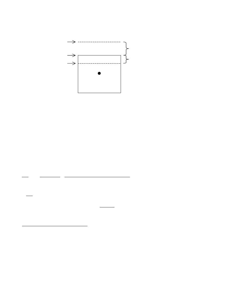
Ground-Water

Flow

Process

Figure 9.-- A model cell for which two storage factors are used during one time step.

i,j,k

TOP

i,j,k

−

Interval over which specific
storage is applied

Interval over which specific yield
is applied

If the head at the beginning of the time step, h

i,j,k

, is below the top of cell i,j,k, so that a free surface exists

within the cell, SCA in equation 38 is set equal to SC2

i,j,k

. If, during an iteration for time step m, the computed

value of head for the end of the time step is below the top of the cell, SCB in the subsequent iteration is also set
equal to SC2

i,j,k

, and equation 38 reverts to the form of equation 37. However, if the computed head for the end of

the time step turns out to be above the top of the cell, SCB in the subsequent iteration is set equal to SC1

i,j,k

, the

confined storage capacity. This situation occurs during intervals of rising water level, and again two components
are computed for the rate of accumulation of water in storage—one corresponding to unconfined or water-table
storage and one corresponding to confined or compressive storage.

Equation 38 can be rearranged as follows:

(

)

TOP

SCB

TOP

SCA

SCB

ûW

û9

−

(39)

Again,

ûW

û9

represents rate of accumulation in storage and as such would appear on the right in equation 2. In the

formulation of equation 3, therefore, the expression

SCB

−

is subtracted from HCOF

i,j,k

on the left-hand side,

while the term

(

)

TOP

SCB

TOP

SCA

−

is added to RHS

i,j,k

on the right-hand side.

For any layer where there is a chance at some point in the simulation that a specific yield should be used

rather than a specific storage at one or more cells, then the convertible option should be used for that layer. When
this is done, values of specific storage for each cell in the layer are read through the variable Ss, and values of
specific yield for each cell in the layer are read through the variable Sy. The specific-storage values are
multiplied times cell volume to obtain confined storage capacity, and the specific-yield values are multiplied by

MODFLOW-2000—User Guide to Modularization Concepts and the

Ground-Water Flow Process

cell area to obtain unconfined storage capacity. Thus, two storage capacities are stored, and the program will use
the appropriate value depending on conditions.

Note that unlike the LPF Package, the BCF Package has a special layer type for a water table in layer 1.

Equation 37 is then used for calculating storage terms. In LPF, the convertible formulation should be used if
layer 1 represents a water table. Also, the elevation of the top of layer 1, which is specified in the discretization
file, should be higher than the water level will reach at any time in the simulation. This will result in equation 38
always reverting to equation 37 as described previously. It is the user’s responsibility in this situation to check to
see that the simulated water level has not exceeded the top elevation, which would trigger the use of confined
storage capacity in equation 38. A logical approach for specifying the top elevation for a layer-1 water table is to
set it equal to land-surface elevation. That is, in most situations, it is not expected that the water table will exceed
land-surface elevation.

Data Requirements

The discretization data—time and space—required by the LPF Package to formulate the flow and storage

terms are specified in the Global Process discretization file. All other data required by LPF are read from the LPF
data file. There are several optional formulations that are controlled by option variables, which have one value for
each layer; that is, the options can be turned on or off on a layer by layer basis. The following option variables are
used by LPF:

LAYCBD—Quasi-3D confining bed flag (read as part of the discretization file),
LAYTYP—Layer-type flag,
LAYAVG—Interblock transmissivity flag,
CHANI—Horizontal anisotropy flag and value,
LAYVKA—Vertical anisotropy flag, and
LAYWET—Wetting flag.

The Quasi-3D confining bed flag (LAYCBD) indicates whether a layer is underlain by a confining bed that is

simulated using the Quasi-3D Approach. This determines how vertical conductance is calculated.

LAYCBD = 0—there is no Quasi-3D confining bed below the layer, so vertical conductance is calculated

using equation 25.

LAYCBD

≠

0—there is a Quasi-3D confining bed below the layer, so vertical conductance is calculated

using equation 27.

The layer-type flag (LAYTYP) indicates whether a layer is confined or convertible (between confined and

unconfined). This controls whether (1) saturated thickness varies with head, (2) storage term conversion is used,
and (3) vertical flow from above is limited under dewatered conditions:

Layer-type flag = 0—The layer is simulated as confined. For a layer of this type, there is no provision for

modification of saturated thickness as head varies, for storage term conversion, or for limitation of
vertical flow from above if the calculated hydraulic head falls below the top of the cell.

Layer-type flag

≠

0—The layer is simulated as convertible between confined and unconfined. When the

calculated hydraulic head is below the top of the cell, all of the options associated with water-table
conditions are implemented. Saturated thickness and transmissivity are recalculated at each iteration
on the basis of head, and both storage term conversion and limitation of flow from above under
dewatered conditions are implemented.

The Interblock transmissivity flag (LAYAVG) indicates the method used for calculating interblock

transmissivity:

Ground-Water

Flow

Process

LAYAVG = 0—Harmonic mean transmissivity is used. This assumes that transmissivity is uniform

within a cell, and that changes occur as discrete changes at cell boundaries.

LAYAVG = 1—logarithmic mean transmissivity is used. This assumes that hydraulic conductivity varies

linearly between nodes.

LAYAVG = 2—arithmetic-mean thickness and logarithmic-mean hydraulic conductivity are used. This is

based on a water-table condition.

The horizontal anisotropy flag (CHANI) indicates whether horizontal anisotropy is constant for a layer, or

whether it can vary at each cell in a layer. In either case, it is assumed that the grid is aligned with the principal
directions of hydraulic conductivity.

CHANI

≤

0.0—Horizontal anisotropy can vary at each cell in the layer. A separate layer-data variable of

the horizontal anisotropy values (HANI) will be read in the input data.

CHANI > 0.0—Horizontal anisotropy is constant for all cells in the layer. The anisotropy is the value of

the flag. For example, set CHANI=1.0 for an isotropic layer.

The vertical anisotropy flag (LAYVKA) indicates the type of values that are specified in variable VKA.

LAYVKA = 0—Values of VKA are vertical hydraulic conductivity of the model layer.

LAYVKA

≠

0—Values of VKA are the ratio of horizontal hydraulic conductivity (along rows) to vertical

hydraulic conductivity for the model layer.

The wetting flag (LAYWET) indicates whether the wetting capability is on or off.

LAYWET = 0—Wetting capability is off.

LAYWET

≠

0—Wetting capability is on for the layer. This is only valid if the layer-type flag indicates

that the layer is convertible (LAYTYP not 0).

Most of the data values that must be specified for the LPF Package are layer data, meaning that the data must

be defined for all cells in one or more of the model layers. As used in the above equations that define the LPF
formulations, all of the layer-data variables have three-dimensional subscripts, indicating that there are values for
all layers; however, some of the variables do not always exist for all layers. The layers for which these layer
variables exist are determined by the values in the above option variables. The layer-data variables defined for use
by LPF are:

HK—horizontal hydraulic conductivity along rows,
HANI—Ratio of horizontal hydraulic conductivity along columns to hydraulic conductivity along rows,
VKA—Vertical hydraulic conductivity or the ratio of horizontal hydraulic conductivity along rows (HK)

to vertical hydraulic conductivity,

VKCB—Vertical hydraulic conductivity of a confining bed below a layer,
Ss—specific storage, and
Sy—-specific yield.
WETDRY—wetting threshold combined with a wetting flag.

HK and VKA are always required for all layers. Ss is required for all layers if there are any transient stress

periods in the simulation. Sy is required for layers in which LAYTYP

≠

0 and if there are any transient stress

periods. The transient/steady-state flags read from the Discretization File determine if storage data are needed.

MODFLOW-2000—User Guide to Modularization Concepts and the

Ground-Water Flow Process

HANI is required for layers in which CHANI

≤

0. VKCB is required for layers in which LAYCBD

≠

WETDRY is required when LAYWET

≠

Defining Layer-Data Variables

The input instructions describe the details of how the LPF input data are read. All of the layer variables can

be directly read by using MODFLOW’s array readers, and variables HK, HANI, VKA, VKCB, SS, and SY can
also be defined by using parameters. The same method of data definition (directly reading or using parameters)
must be used for all the layers for a given variable; that is, some of the layers of a particular variable cannot be
directly read if some of the layers are defined through parameters and conversely.

When the array readers are used, any of the unused layer data that are included in the input file will cause the

data sequence to be misread. Likewise, if any of the required layer arrays are left out of the input file, the data
sequence will be misread.

When variables are defined by using array readers, a value must be specified for every cell even if the value

will not be used; that is, the array readers read a value for each cell regardless of whether or not the value will be
used. For no-flow cells, the values of variables are never used in any calculation, and thus any values may be
specified; for constant-head cells, the Ss, Sy, and WETDRY variables are not used but the other variables are.

When variables are defined by using parameters, it is required that a value is defined for variable-head cells

(IBOUND > 0) and constant-head cells (IBOUND < 0). If a value is not assigned at one or more variable- or
constant-head cells, then the program will print an error message and stop.

MODFLOW-96 to MODFLOW-2000 Data Conversion Program

MF96TO2K is a utility program that converts MODFLOW-96 input data to MODFLOW-2000 input data. To

convert a MODFLOW-96 data set to run with MODFLOW-2000, MF96TO2K reads three files and produces four
files: it reads the MODFLOW-96 name, BAS, and BCF files; it produces the discretization file and modified
versions of the name, BCF, and BAS files. For confining beds and confined model layers for which top and
bottom elevations are not included in the MODFLOW-96 BCF file, MF96TO2K queries the user for these values.
Only constant elevation values for each layer can be specified; if non-constant values are required, the user needs
to modify the discretization file after it is created by MF96TO2K.

The additional elevation data that MF96TO2K requires in order to create the discretization file are not used

by the BCF Package and have no affect on simulation results unless the Horizontal-Flow Barrier Package is being
used. The reason these additional values do not affect the BCF Package is that many of the BCF input values
directly incorporate the geometry of the system as discussed in the section of this report on the BCF Package. The
only elevation data that affect the BCF calculations are the values from the MODFLOW-96 BCF file, which
MF96TO2K puts into MODFLOW-2000’s discretization file.

The MODFLOW-2000 version of HFB makes use of the additional elevation data that MF96TO2K requests

for the discretization file when there are barriers in confined layers. As previously mentioned, if the additional
data are not constant for a layer, the user must modify the discretization file after running MF96TO2K. Further, if
the Horizontal-Flow Barrier (HFB) Package is used, its input data must be modified, and MF96TO2K does not
make this modification.

MF96TO2K functions as follows.

1. It starts by asking for a MODFLOW-96 name file.

2. It then uses this to open the files needed for data conversion.

3. Next, it asks if each layer (except the bottom layer) has a Quasi-3D confining bed under it.

4. It then asks for a constant elevation for any model layers for which elevation data are not included in the

MODFLOW-96 BCF file.

5. Finally, MF96TO2K creates new BAS and BCF files using file name extensions BA6 and BC6, respectively.

MF96TO2K also creates a discretization file and it overwrites the name file.

After conversion, MODFLOW-2000 should produce the same results as MODFLOW-96 produced.

Input

Instructions

Adding Packages

As noted in the Introduction section, MODFLOW was originally designed with the goal of making it easy to

add new capabilities. The addition of packages is the typical way of enhancing MODFLOW. Packages can be
added to the Ground-Water Flow Process of MODFLOW-2000 in much the same way as they could be added to
the original versions of MODFLOW. In fact, most packages that have been added to earlier versions of
MODFLOW can be added to the Ground-Water Flow Process of MODFLOW-2000 with no change. However,
there would probably be an advantage to modifying some packages to include parameters. The most likely cause
for an existing package to no longer work in MODFLOW-2000 is the new way in which cell elevations are
handled. That is, any package that relies on elevation data as specified in the old BCF Package will require some
modification. Another cause for a package to no longer work is the new ability to intermix steady-state and
transient stress periods. Examples of packages that require modification are the Transient-leakage (TLK) Package
(Leake and others, 1994), the General Finite-Difference Flow (GFD) Package (Harbaugh, 1992), and the Interbed-
Storage (IBS) Package (Leake and Prudic, 1991). Examples of packages that require no modification to include in
MODFLOW-2000 are the Reservoir (RES) package (Fenske and others, 1996) and the Flow and Head Boundary
(FHB) Package (Leake and Lilly, 1997).

Note that packages added to the Ground-Water Flow Process are not necessarily compatible with other

processes. There would likely be benefit from adding most hydrologic packages to other processes within
MODFLOW-2000, but this is beyond the scope of this report. The documentation for new packages should
include information about the processes that they work with. Previously developed packages must be evaluated to
determine compatibility with other processes, and the documentation of new processes should describe the degree
of compatibility with existing packages to the extent possible.

INPUT INSTRUCTIONS

Input instructions for MODFLOW-2000 are divided into four major sections: Global Process, Ground-Water

Flow Process, Array Utility Modules, and List Utility Module. The Global Process reads several files, and each
file is described in a separate subsection. The Ground-Water Flow Process reads at least one file for each package,
and these files are also described separately. The instructions for a file are grouped by numbered items, and each
item consists of input variables. If a variable is represented in the program by a variable of the same name, then
the variable is shown in all upper case. Variables that are not actual program variables are capitalized. Each
variable is defined after all the items are listed.

An input variable may include a single value or multiple values. One-dimensional variables are multi-valued

variables in which the number of values is indicated by a single number in parentheses after the name. Two-
dimensional variables are multi-valued variables in which the number of values is indicated by two numbers in
parentheses after the name. The total number of values represented is the product of the two numbers. A layer
variable is a two-dimensional variable that includes one value for each cell in a layer. Therefore, the column and
row dimensions are the numbers in parentheses after the variable. For example, "IBOUND(NCOL,NROW)"
indicates that IBOUND is a layer variable. Most multi-value variables are read by utility modules, and if so, the
utility module (U1DREL, U2DREL, or U2DINT) is named along with the variable. Module U1DREL is used for
reading one-dimensional variables that are real numbers, U2DREL is used for reading two-dimensional variables
that are real numbers, and U2DINT is used for reading two-dimensional variables that are integer numbers.

Some items consist of several variables, and the item can be repeated multiple times. This kind of item is

called a list item. List items are usually read by the list utility module, ULSTRD. The use of ULSTRD is
mentioned as part of the note that describes the repeated item.

The input data for each item must start on a new record. (A record is a line in a file.) It is assumed that all

variables for an item will be contained in a single record unless the item consists of a multi-valued variable. That
is, a multi-valued variable may occupy multiple records. When reading a layer variable, the data for each row
must start on a new record.

MODFLOW-2000—User Guide to Modularization Concepts and the

Ground-Water Flow Process

Each input variable has a data type, which can be Real, Integer, or Character. Integers are whole numbers,

and these values must not include a decimal point or exponent. Real numbers can include a decimal point and an
exponent. If no decimal point is included in the entered value, then the decimal point is assumed to be at the right
side of the value. Any printable character is allowed for character variables. All variables starting with the letters
I-N are integers. Variables starting with the letters A-H and O-Z are either real numbers or character data, and
most of these variables are real numbers; that is, there are few character variables in MODFLOW. It should be
assumed that a variable starting with A-H or O-Z is a real number unless otherwise stated in the variable
definitions. This data-type convention is used for all input variables regardless of whether a variable is an actual
program variable.

Both free and fixed formatting are used as specified throughout the input instructions. With fixed format, a

data value has a specified column location, called the field, within a record. If a numeric value does not require
the entire field width, the value should be right justified within the field, and blanks should fill the remaining
width of the field. The justification of character data within a field does not matter unless specifically noted.

Free format is similar to Fortran’s list directed input. With free format, values are not required to occupy a

fixed number of columns in a record. Each value can occupy one or more columns as required to represent it;
however, the values must still be included in the prescribed order. One or more spaces, or a single comma
optionally combined with spaces, must separate adjacent values. Also, a numeric value of zero must be explicitly
represented with 0 and not by one or more spaces when free format is used, because there is no way to detect the
difference between a space that represents 0 and a space that represents a value separator.

Two capabilities included in Fortran’s list-directed input are not included in the free-format input

implemented in MODFLOW-2000.

1. Null values in which input values are left unchanged from their previous values are not allowed. In general,

MODFLOW’s input values are not defined prior to their input.

2. A "/" cannot be used to terminate an input record without including values for all the variables; data values for

all input variables must be explicitly specified on an input record.

For character data, MODFLOW’s free format implementation is less stringent than the list-directed input of

Fortran 77. Fortran requires character data to be delineated by apostrophes. MODFLOW does not require
apostrophes unless a blank or a comma is part of a character variable.

An example problem is included in the Example section. That section shows input files that illustrate the use

of parameters.

Running MODFLOW-2000

MODFLOW-2000 is executed in the same manner as MODFLOW-96. Except as described in the following

paragraphs, when MODFLOW-2000 is started, it prompts the user to enter the name of the name file, which is
described below. Once the name is entered, MODFLOW-2000 runs without further user interaction.

Provision has been made to allow a series of simulations to be run without the need to manually restart

MODFLOW-2000 for each simulation and respond to the prompt for the name file. This is called batch mode and
is done through the use of a special file that must be named modflow.bf. On case-sensitive operating systems,
such as Unix, lower case letters are needed. If a file with this name exists in the user’s current directory when
MODFLOW-2000 is invoked, the user is not prompted for a name file. Instead, MODFLOW-2000 reads the
names of name files from modflow.bf. Each line of the modflow.bf file contains the name of a single name file,
and each name can be up to 80 characters long.

When batch mode is used, a report file, named modbatch.rpt, is created. Before starting a simulation, the

name of the name file is written to the report file. If the name file exists, the simulation is executed; when done,
another message is written to the report file. If a name file does not exist, a message is written to the report file
and processing continues with the next name file in modflow.bf.

When batch mode is used to run MODFLOW-2000, two additional file units are used—97 and 98. These

units cannot be used by any of the MODFLOW-2000 simulations. Within the name files listed in modflow.bf, the

Input

Instructions

file units listed in one name file can be the same as those used in any of the other name files because each
simulation is executed separately.

Global Process Input Instructions

Name File

The name file contains the names of most input and output files used in a model simulation and controls the

parts of the model program that are active. (“OPEN/CLOSE” files, described in the Input Instructions for Array
Reading Utility Modules section, are not included in the name file.) The name file is read on unit 99. The name
file is constructed as follows.

FOR EACH SIMULATION

1. Ftype Nunit Fname

The name file contains one of the above records (item 1) for each file. All variables are free format. The
length of each record must be 199 characters or less. The records can be in any order except for records
where Ftype (file type) is “GLOBAL” or “LIST” as described below.

Comment records are indicated by the # character in column one and can be located anywhere in the file.
Any text characters can follow the # character. Comment records have no effect on the simulation; their
purpose is to allow users to provide documentation about a particular simulation. All comment records
after the first item-1 record are written in the listing file.

Explanation of Variables in the Name File

Ftype—is the file type, which must be one of the following character values. Ftype may be entered in all
uppercase, all lowercase, or any combination.

GLOBAL for the global listing file—if this type is not present, the LIST file is used for the

global listing file as well as for the forward run listing file.

LIST for the forward run listing file—if this type is not present, the GLOBAL file is used for the

forward run listing file as well as for the global listing file.

The name file must always include a record that specifies GLOBAL or LIST for Ftype.
Both records can be included, and if so, the GLOBAL record must be the first non-
comment record and the LIST record must be the second non-comment record. If only one
of the records is included, it must be the first non-comment record.

DIS for the discretization file
MULT for the multiplier array file
ZONE for the zone array

BAS6 for the Ground-Water Flow Process Basic Package
OC for the Ground-Water Flow Process Output Control Option
BCF6 for the Ground-Water Flow Process Block-Centered Flow Package
LPF for the Ground-Water Flow Process Layer Property Flow package
HFB6 for the Ground-Water Flow Process Horizontal Flow Barrier Package
RCH for the Ground-Water Flow Process Recharge Package
RIV for the Ground-Water Flow Process River Package
WEL for the Ground-Water Flow Process Well Package

MODFLOW-2000—User Guide to Modularization Concepts and the

Ground-Water Flow Process

DRN for the Ground-Water Flow Process Drain Package
GHB for the Ground-Water Flow Process General-Head Boundary Package
EVT for the Ground-Water Flow Process Evapotranspiration Package
CHD for the Ground-Water Flow Process Constant-Head Package

SIP for the Strongly Implicit Procedure Package
SOR for the Slice-Successive Over-Relaxation Package
PCG for the Preconditioned Conjugate-Gradient Package
DE4 for the Direct Solution Package

DATA(BINARY) for binary (unformatted) files, such as those used to save cell-by-cell budget data and

binary (unformatted) head and drawdown data. Files of this type are rewound at the start of each
parameter-estimation iteration.

DATA for formatted (text) files, such as those used to save formatted head and drawdown and for input of

data from files that are separate from the primary package input files. Files of this type are rewound at
the start of each parameter-estimation iteration.

DATAGLO(BINARY) for binary (unformatted) files, such as those used to save cell-by-cell budget data

and binary (unformatted) head and drawdown data. Files of this type are not rewound at the start of
each parameter-estimation iteration;. that is, output from each successive parameter iteration
accumulates rather than overwriting information from the previous iteration.

DATAGLO for formatted (text) files, such as those used to save formatted head and drawdown and for

input of data from files that are separate from the primary package input files. Files of this type are not
rewound at the start of each parameter-estimation iteration; that is, output from each successive
parameter iteration accumulates rather than overwriting information from the previous iteration.

Nunit—is the Fortran unit to be used when reading from or writing to the file. Any legal unit number on the
computer being used can be specified except units 96-99. Unit 99 is used for the name file and for reading multi-
valued variables using the OPEN/CLOSE option of the utility modules (see Input Instructions for Array Reading
Utility Modules section). Units 97 and 98 are used for batch files as explained below. Unit 96 is used for a file to
which error messages may be written when the Sensitivity Process is active. The unit number for each file must
be unique.

Fname—is the name of the file, which is a character value. Pathnames may be specified as part of Fname.

Input

Instructions

Discretization File

Discretization information is read from the file that is specified by "DIS" as the file type.

FOR EACH SIMULATION

0. [#Text]

Item 0 is optional—“#” must be in column 1. Item 0 can be repeated multiple times.

1. NLAY

NROW

NCOL

NPER

ITMUNI

LENUNI

2. LAYCBD(NLAY)
3. DELR(NCOL) - U1DREL
4. DELC(NROW) - U1DREL
5. Top(NCOL,NROW) - U2DREL
6. BOTM(NCOL,NROW) - U2DREL

Item 6 is repeated for each model layer and Quasi-3D confining bed in the grid. These layer variables are
read in sequence going down from the top of the system. Thus, the number of BOTM arrays must be
NLAY plus the number of Quasi-3D confining beds.

FOR EACH STRESS PERIOD

7. PERLEN NSTP TSMULT Ss/tr

Explanation of Variables Read from the Discretization File

0 - undefined 3 - hours
1 - seconds 4 - days
2 - minutes 5 - years

LENUNI—indicates the length unit of model data, which must be consistent for all data values that involve
length. For example, if feet is the chosen length unit, grid spacing, head, hydraulic conductivity, water volumes,
and so forth, must all be expressed using feet for their length units. Note that the program will still run even if
“undefined” length units are specified because the fundamental equations used in MODFLOW do not require that
the length unit be identified. But be sure to use consistent units for all input data even when LENUNI indicates an
undefined length unit:

0 - undefined
1 - feet

MODFLOW-2000—User Guide to Modularization Concepts and the

Ground-Water Flow Process

2 - meters
3 - centimeters

LAYCBD—is a flag, with one value for each model layer, that indicates whether or not a layer has a Quasi-3D
confining bed below it. 0 indicates no confining bed, and not zero indicates a confining bed. LAYCBD for the
bottom layer must be 0.

DELR—is the cell width along rows. Read one value for each of the NCOL columns. This is a multi-value one-
dimensional variable with one value for each column.

DELC—is the cell width along columns. Read one value for each of the NROW rows. This is a multi-value one-
dimensional variable with one value for each row.

Top—is the top elevation of layer 1. For the common situation in which the top layer represents a water-table
aquifer, it may be reasonable to set Top equal to land-surface elevation.

BOTM—is the bottom elevation of a model layer or a Quasi-3d confining bed.

PERLEN—is the length of a stress period.

NSTP—is the number of time steps in a stress period.

TSMULT—is the multiplier for the length of successive time steps. The length of a time step is calculated by
multiplying the length of the previous time step by TSMULT. The length of the first time step,

∆

, is related to

PERLEN, NSTP, and TSMULT by the relation













TSMULT

PERLEN

ûW

NSTP

Ss/tr—is a character variable that indicates if the stress period is transient or steady state. The only allowed
options are “SS” and “TR”, but these are case insensitive.

Input

Instructions

Multiplier File

Input to define multiplier arrays is read from the file that is specified with "MULT" as the file type.

Multiplier arrays can be used to calculate layer variables from parameter values.

FOR EACH SIMULATION

0. [#Text]

Item 0 is optional—“#” must be in column 1. Item 0 can be repeated multiple times.

1. NML

2. MLTNAM [

FUNCTION]

If Item 2 does not contain the optional

FUNCTION

keyword, read Item 3:

3. [RMLT(NCOL,NROW)] - U2DREL

Otherwise, if Item 2 contains the optional

FUNCTION

keyword, read Item 4:

4. [MLTNAM1 [op1 MLTNAM2] [op2 MLTNAM3] [op3 MLTNAM4] ... ]

Repeat items 2-4 for each of the NML multiplier arrays.

Explanation of Variables Read from the Multiplier File

Example Multiplier Array Input Using the FUNCTION Keyword

The following example input illustrates the use of the FUNCTION keyword to construct a multiplier array

from other multiplier arrays. In this example, three multiplier arrays are defined. The first two arrays (named M1
and M2) are read using the U2DREL utility array reader (item 3), and the third array (named M3) is defined as the
sum of the other two. In this example, a model layer has 5 rows and 4 columns.

MODFLOW-2000—User Guide to Modularization Concepts and the

Ground-Water Flow Process

INTERNAL 1.0 (4F6.0) 0

1.0 1.1 1.2 1.3

2.0 2.2 2.4 2.6

1.0 1.1 1.2 1.3

INTERNAL 1.0 (4F6.0) 0

5.0 5.1 5.2 5.3

6.0 6.1 6.2 6.3

5.0 5.1 5.2 5.3

M3 FUNCTION

M1 + M2

The resulting values for multiplier M3 are:

6.0 6.2 6.4 6.6

8.0 8.3 8.6 8.9

6.0 6.2 6.4 6.6

Input

Instructions

Zone File

Input to define zone arrays is read from the file that is specified with "ZONE" as the file type. Zone arrays

can be used to specify the cells in a layer variable that are associated with a parameter.

FOR EACH SIMULATION

0. [#Text]

Item 0 is optional—“#” must be in column 1. Item 0 can be repeated multiple times.

1. NZN

2. ZONNAM
3. IZON(NCOL,NROW) - U2DINT

Items 2-3 are repeated for each of the NZN zone arrays.

Explanation of Variables Read from the Zone File

MODFLOW-2000—User Guide to Modularization Concepts and the

Ground-Water Flow Process

Ground-Water Flow Process Input Instructions

Basic Package

Input for the Ground-Water Flow Process Basic (BAS) Package except for output control input is read from

the file that is specified with “BAS6” as the file type. The file type has been changed from that used in
MODFLOW-96, which was “BAS”, because the input data are not compatible.

FOR EACH SIMULATION

0. [#Text]

Item 0 is optional—“#” must be in column 1. Item 0 can be repeated multiple times.

1. Options (199 text characters)

If there are no options to specify, then a blank record must be included for Item 1.

2. IBOUND(NCOL,NROW) or (NCOL,NLAY) -- U2DINT

If not a cross section, a layer variable is read for each layer in the grid.
If a cross section, NLAY rows of NCOL values are read.

3. HNOFLO (10-character field unless Item 1 contains ‘FREE’.)

4. STRT(NCOL,NROW) or (NCOL,NLAY) -- U2DREL

If not a cross section, a layer variable is read for each layer in the grid.
If a cross section, NLAY rows of NCOL values are read.

Explanation of Variables Read by the BAS Package

Text—is a character variable that starts in column 2. The first two comment lines will become variable
HEADNG, which is used as a printout title throughout the program. (If there are no comment lines, then
HEADNG will be blank.) HEADNG is limited to 80 columns, but subsequent Text lines can be up to 199
columns. Any characters can be included in Text. The “#” character must be in column 1. Except for the name
file, lines beginning with # are restricted to these first lines of the file. Text is printed when the file is read.

Options—is a character variable that is scanned for words (separated by one or more spaces) that specify program
options. Three options are currently recognized. Unrecognized words are ignored, and a word may be specified in
either uppercase or lowercase. A blank record is acceptable and indicates no options.

XSECTION indicates that the model is a 1-row cross section for which STRT and IBOUND should each

be read as single two-dimensional variables with dimensions of NCOL and NLAY. Likewise, head
and drawdown should be printed and saved in disk files as single two-dimensional variables.

CHTOCH indicates that flow between adjacent constant-head cells should be calculated.

FREE indicates that free format is used for input variables throughout the Basic Package and other

packages as indicated in their input instructions. Be sure that all variables read using free format have
a non-blank value and that a comma or at least one blank separates all adjacent values.

IBOUND—is the boundary variable. One value is read for every model cell. Usually, these values are read a layer
at a time; however, when the XSECTION option is specified, a single variable for the cross section is read. Note

Input

Instructions

that although IBOUND is read as one or more two-dimensional variables, it is stored internally as a three-
dimensional variable.

If IBOUND(J,I,K) < 0, cell J,I,K has a constant head.
If IBOUND(J,I,K) = 0, cell J,I,K is inactive.
If IBOUND(J,I,K) > 0, cell J,I,K is active.

HNOFLO—is the value of head to be assigned to all inactive (no flow) cells (IBOUND = 0) throughout the
simulation. Because head at inactive cells is unused in model calculations, this does not affect model results but
serves to identify inactive cells when head is printed. This value is also used as drawdown at inactive cells if the
drawdown option is used. Even if the user does not anticipate having inactive cells, a value for HNOFLO must be
entered.

STRT—is initial (starting) head—that is, head at the beginning of the simulation. STRT must be specified for all
simulations, including steady-state simulations. One value is read for every model cell. Usually, these values are
read a layer at a time. When the XSECTION option is specified, however, a single array for the cross section is
read. For simulations in which the first stress period is steady state, the values used for STRT generally do not
affect the simulation (exceptions may occur if cells go dry and(or) rewet). The execution time, however, will be
less if STRT includes hydraulic heads that are close to the steady-state solution.

MODFLOW-2000—User Guide to Modularization Concepts and the

Ground-Water Flow Process

Output Control Option

Input to the Output Control Option of the Ground-Water Flow Process is read from the file that is specified

as type "OC" in the name file. If no "OC" file is specified, default output control is used. Under the default, head
and overall budget are written to the listing file (printed) at the end of every stress period. The default printout
format for head and drawdown is 10G11.4.

There are two ways to specify Output Control data: words or numeric codes. One of these methods must be

used throughout any simulation.

Output Control Using Words

Recognized words are shown in bold italics; these words must be entered exactly as shown except that
they may be entered in either uppercase or lowercase. Optional parts of records are shown in brackets.
One or more spaces must separate each word or variable, and the total record length must not exceed 199
characters.

FOR EACH SIMULATION

0. [#Text]
Item 0 is optional—“#” must be in column 1. Item 0 can be repeated multiple times.

1. Any combination of the following records:

HEAD PRINT FORMAT IHEDFM

HEAD SAVE FORMAT CHEDFM [LABEL]

Omit to obtain an unformatted file.

HEAD SAVE UNIT IHEDUN

DRAWDOWN PRINT FORMAT IDDNFM

DRAWDOWN SAVE FORMAT CDDNFM [LABEL]

Omit to obtain an unformatted file.

DRAWDOWN SAVE UNIT IDDNUN

IBOUND SAVE FORMAT CBOUFM [LABEL]

IBOUND SAVE UNIT IBOUUN

COMPACT BUDGET [AUX or AUXILIARY]

If the final “

COMPACT BUDGET

” option is used, cell-by-cell budget files produced require less disk

space than files written by MODFLOW-88; however, programs that read these data using the
specifications of MODFLOW-88 will need to be modified. If this option is not used, MODFLOW-2000
will write the files using the MODFLOW-88 method. The optional word “AUX” (or “AUXILIARY”)
after “COMPACT BUDGET” indicates that auxiliary data that are defined in packages (see input data for
the RIV, WEL, DRN, and GHB Packages) should be saved in the budget file along with budget data.

PRINT

indicates that the model output is written to the LIST file.

SAVE

indicates that output is written to the indicated file unit. Drawdown and head are saved as text files

if the

SAVE FORMAT

record is included. If the

SAVE FORMAT

record is not used, then the file is written

as a binary (unformatted) file. Binary files are usually more compact than text files, but they are not
generally transportable among different computer operating systems or different Fortran compilers.

FOR EACH TIME STEP FOR WHICH OUTPUT IS DESIRED

PERIOD IPEROC STEP ITSOC

3. Any combination of the following records:

PRINT HEAD [list layers if all layers not desired]

PRINT DRAWDOWN [list layers if all layers not desired]

Input

Instructions

PRINT BUDGET

Write overall volumetric budget to the LIST file.

SAVE HEAD [list layers if all layers not desired]

SAVE DRAWDOWN [list layers if all layers not desired]

SAVE IBOUND [list layers if all layers not desired]

SAVE BUDGET

Write cell-by-cell budget data to a file.

Item 2 and one or more item-3 records are specified for each time for which output is desired. These
records must be in the order of increasing simulation time.

Explanation of Variables Read by Output Control Using Words

0 - 10G11.4 11 - 20F5.4
1 - 11G10.3 12 - 10G11.4
2 - 9G13.6 13 - 10F6.0
3 - 15F7.1 14 - 10F6.1
4 - 15F7.2 15 - 10F6.2
5 - 15F7.3 16 - 10F6.3
6 - 15F7.4 17 - 10F6.4
7 - 20F5.0 18 - 10F6.5
8 - 20F5.1 19 - 5G12.5
9 - 20F5.2 20 - 6G11.4

10 - 20F5.3 21 - 7G9.2

CHEDFM—is a character value that specifies the format for saving heads, and can only be specified if the word
method of output control is used. The format must contain 20 characters or less and must be a valid Fortran
format that is enclosed in parentheses. The format must be enclosed in apostrophes if it contains one or more
blanks or commas. The optional word

LABEL

after the format is used to indicate that each layer of output should

be preceded with a line that defines the output (simulation time, the layer being output, and so forth). If there is no
record specifying CHEDFM, then heads are written to a binary (unformatted) file. Binary files are usually more
compact than text files, but they are not generally transportable among different computer operating systems or
different Fortran compilers.

IHEDUN—is the unit number on which heads will be saved.

IDDNFM—is a code for the format in which drawdowns will be printed. The codes are the same as for IHEDFM.

CDDNFM—is a character value that specifies the format for saving drawdown, and can only be specified if the
word method of output control is used. The format must contain 20 characters or less and must be a valid Fortran
format that is enclosed in parentheses. The format must be enclosed in apostrophes if it contains one or more
blanks or commas. The optional word

LABEL

after the format is used to indicate that each layer of output should

be preceded with a line that defines the output (simulation time, the layer being output, and so forth). If there is no
record specifying CDDNFM, then drawdown is written to a binary (unformatted) file. Binary files are usually
more compact than text files, but they are not generally transportable among different computer operating systems
or different Fortran compilers.

IDDNUN—is the unit number on which drawdowns will be saved.

CBOUFM—is a character value that specifies the format for saving IBOUND, and can only be specified if the
word method of output control is used. The format must contain 20 characters or less and must be a valid Fortran
format that is enclosed in parentheses. The format must be enclosed in apostrophes if it contains one or more
blanks or commas. The optional word

LABEL

is used to indicate that each layer of output should be preceded

with a line that defines the output (simulation time, the layer being output, and so forth). If there is no record

MODFLOW-2000—User Guide to Modularization Concepts and the

Ground-Water Flow Process

specifying CBOUFM, then IBOUND is written using format (20I4). IBOUND is never written as a binary
(unformatted) file.

IBOUUN—is the unit number on which drawdowns will be saved.

IPEROC—is the stress period number at which output is desired.

ITSOC—is the time step number (within a stress period) at which output is desired.

Example Output Control Input Using Words

The first line cannot be blank, but after the first line blank lines are ignored when the word method is used to

specify Output Control data. Indented lines are allowed because of the use of free format input.

HEAD PRINT FORMAT 15
HEAD SAVE FORMAT (20F10.3) LABEL
HEAD SAVE UNIT 30
COMPACT BUDGET FILES
DRAWDOWN PRINT FORMAT 14

PERIOD 1 STEP 1
PRINT HEAD 2 6
PRINT DRAWDOWN
PRINT BUDGET
SAVE BUDGET
SAVE HEAD

PERIOD 1 STEP 7
SAVE HEAD 1 3 5
PRINT DRAWDOWN
SAVE BUDGET

PERIOD 2 STEP 5
PRINT HEAD
PRINT BUDGET
SAVE BUDGET
SAVE HEAD

Output Control Using Numeric Codes

All variables are free format if the word FREE is specified in Item 1 of the Basic Package input file;

otherwise, the variables all have 10-character fields.

FOR EACH SIMULATION

0. [#Text]
Item 0 is optional—“#” must be in column 1. Item 0 can be repeated multiple times.

1. IHEDFM IDDNFM IHEDUN IDDNUN

FOR EACH TIME STEP

2. INCODE IHDDFL IBUDFL ICBCFL
3. Hdpr Ddpr Hdsv Ddsv

(Item 3 is read 0, 1, or NLAY times, depending on the value of INCODE.)

Input

Instructions

Explanation of Variables Read by Output Control Using Numeric Codes

If INCODE < 0, Item 3 flags are used from the last time step. Item 3 is not read.
If INCODE = 0, all layers are treated the same way. Item 3 will consist of one record.
If INCODE > 0, Item 3 will consist of one record for each layer.

IHDDFL—is a head and drawdown output flag. This flag allows Item 3 flags to be specified in an early time step
and then used or not used in subsequent time steps. Thus, it may be possible to use IHDDFL to avoid resetting
Item 3 flags every time step.

If IHDDFL = 0, no heads or drawdowns will be printed or saved regardless of which Item 3 flags are

specified.

If IHDDFL

≠

0, heads and drawdowns will be printed or saved according to the Item 3 flags.

IBUDFL—is a budget print flag.

If IBUDFL = 0, overall volumetric budget will not be printed.

If IBUDFL

≠

0, overall volumetric budget will be printed.

ICBCFL—is a flag for writing cell-by-cell flow data.

If ICBCFL = 0, cell-by-cell flow terms are not written to any file.

If ICBCFL

≠

0, cell-by-cell flow terms are written to the LIST file or a budget file depending on flags set

in the component of flow packages, that is, IWELCB, IRCHCB, and so forth.

Hdpr—is the output flag for head printout.

If Hdpr = 0, head is not printed for the corresponding layer.

If Hdpr

≠

0, head is printed for the corresponding layer.

Ddpr—is the output flag for drawdown printout.

If Ddpr = 0, drawdown is not printed for the corresponding layer.

If Ddpr

≠

0, drawdown is printed for the corresponding layer.

Hdsv—is the output flag for head save.

If Hdsv = 0, head is not saved for the corresponding layer.

If Hdsv

≠

0, head is saved for the corresponding layer.

Ddsv—is the output flag for drawdown save.

If Ddsv = 0, drawdown is not saved for the corresponding layer.

If Ddsv

≠

0, drawdown is saved for the corresponding layer.

MODFLOW-2000—User Guide to Modularization Concepts and the

Ground-Water Flow Process

Block-Centered Flow Package

This version of the Block-Centered Flow (BCF) Package combines the capabilities documented in McDonald

and Harbaugh (1988), McDonald and others (1992), and Goode and Appel (1992). Input for the BCF Package is
read from the file that is type "BCF6" in the name file. The file type has been changed from that used in
MODFLOW-96, which was “BCF”, because the input data are not compatible.

FOR EACH SIMULATION

1. IBCFCB HDRY IWDFLG WETFCT IWETIT IHDWET

These 6 variables are free format if the option “FREE” is specified in the Basic Package input file;
otherwise, the variables all have 10-character fields.

2. Ltype(NLAY)

Read one value for each layer. These values are free format if the word FREE is specified in Item 1 of the
Basic Package input file; otherwise, they have fixed-format fields. The fixed format fields are each 2
characters wide with 40 values per line. Use only as many lines as required for the number of model
layers.

3. TRPY(NLAY) -- U1DREL

A subset of the following two-dimensional variables are used to describe each layer. The variables needed for

each layer depend on the layer-type code (LAYCON, which is defined as part of the Item-2 Ltype), whether the
simulation has any transient stress periods (at least one stress period defined in the Discretization File specifies
Ss/Tr as “TR”), and if the wetting capability is active (IWDFLG not 0). If a variable is not needed, it must be
omitted. In no situation will all variables be required. The required variables (Items 4-9) for layer 1 are read first;
then the variables for layer 2 and so forth.

4. [Sf1(NCOL,NROW)]-- U2DREL

If there is at least one transient stress period.

If LAYCON is 0 or 2 (see Ltype ), then read item 5.

5. [Tran(NCOL,NROW)] -- U2DREL

Otherwise, if LAYCON is 1 or 3 (see Ltype), read item 6.

6. [HY(NCOL,NROW)] -- U2DREL

7. [Vcont(NCOL,NROW)] -- U2DREL

If not the bottom layer.

8. [Sf2(NCOL,NROW)] -- U2DREL

If there is at least one transient stress period and

LAYCON

(see

Ltype)

9. [WETDRY(NCOL,NROW)] -- U2DREL

If IWDFLG is not 0 and LAYCON

(see

Ltype).

Explanation of Variables Read by the BCF Package

IBCFCB—is a flag and a unit number.

If IBCFCB > 0, it is the unit number to which cell-by-cell flow terms will be written when "SAVE

BUDGET" or a non-zero value for ICBCFL is specified in Output Control. The terms that are saved
are storage, constant-head flow, and flow between adjacent cells.

If IBCFCB = 0, cell-by-cell flow terms will not be written.
If IBCFCB < 0, cell-by-cell flow for constant-head cells will be written in the listing file when "SAVE

BUDGET" or a non-zero value for ICBCFL is specified in Output Control. Cell-by-cell flow to storage
and between adjacent cells will not be written to any file.

Input

Instructions

IWDFLG—is a flag that determines if the wetting capability is active.

If IWDFLG = 0, the wetting capability is inactive.
If IWDFLG is not 0, the wetting capability is active.

WETFCT—is a factor that is included in the calculation of the head that is initially established at a cell when it is
converted from dry to wet. (See IHDWET.)

IWETIT—is the iteration interval for attempting to wet cells. Wetting is attempted every IWETIT iteration. If
using the PCG solver (Hill, 1990), this applies to outer iterations, not inner iterations. If IWETIT is 0, it is
changed to 1.

IHDWET—is a flag that determines which equation is used to define the initial head at cells that become wet:

If IHDWET = 0, equation 33A (equation 3a in McDonald and others, 1992) is used:

h = BOT + WETFCT (h

- BOT)

If IHDWET is not 0, equation 33B (equation 3b in McDonald and others, 1992) is used:

h = BOT + WETFCT (WETDRY)

Ltype—contains a combined code for each layer that specifies both the layer type (LAYCON) and the method of
computing interblock conductance. Use as many records as needed to enter a value for each layer. Values are two-
digit numbers:

The left digit defines the method of calculating interblock transmissivity. The methods are described by
Goode and Appel (1992).

0 or blank—harmonic mean (the method used in MODFLOW-88).
1—arithmetic mean
2—logarithmic mean
3—arithmetic mean of saturated thickness and logarithmic-mean hydraulic conductivity.

The right digit defines the layer type (LAYCON), which is the same as in MODFLOW-88:

0—confined—Transmissivity and storage coefficient of the layer are constant for the entire simulation.
1—unconfined—Transmissivity of the layer varies. It is calculated from the saturated thickness and

hydraulic conductivity. The storage coefficient is constant. This type code is valid only for layer 1.

2—confined/unconfined—Transmissivity of the layer is constant. The storage coefficient may alternate

between confined and unconfined values. Vertical flow from above is limited if the layer desaturates.

3—confined/unconfined—Transmissivity of the layer varies. It is calculated from the saturated thickness

and hydraulic conductivity. The storage coefficient may alternate between confined and unconfined
values. Vertical flow from above is limited if the aquifer desaturates.

TRPY—is a one-dimensional variable containing a horizontal anisotropy factor for each layer. It is the ratio of
transmissivity or hydraulic conductivity (whichever is being used) along a column to transmissivity or hydraulic
conductivity along a row. Set to 1.0 for isotropic conditions. This is a single variable with one value per layer. Do
not read a variable for each layer—that is, include only one array control record for the entire variable. Note that
the LPF Package can be used to represent horizontal anisotropy that varies in magnitude within a model layer.

MODFLOW-2000—User Guide to Modularization Concepts and the

Ground-Water Flow Process

Sf1—is the primary storage coefficient. Read only if there are one or more transient stress periods specified in the
Discretization File. For LAYCON equal to 1, Sf1 will always be specific yield, whereas for LAYCON equal to 2
or 3, Sf1 will always be confined storage coefficient. For LAYCON equal to 0, Sf1 would normally be confined
storage coefficient; however, a LAYCON value of 0 can also be used to simulate water-table conditions where
drawdowns are expected to remain everywhere a small fraction of the saturated thickness, and where there is no
layer above, or flow from above is negligible. In this case, specific yield values would be entered for Sf1.

Tran—is the transmissivity along rows. Tran is multiplied by TRPY to obtain transmissivity along columns. Read
only for layers where LAYCON is 0 or 2.

HY—is the hydraulic conductivity along rows. HY is multiplied by TRPY to obtain hydraulic conductivity along
columns. Read only for layers where LAYCON is 1 or 3.

Vcont—is the vertical hydraulic conductivity divided by the thickness from a layer to the layer below. The value
for a cell is the hydraulic conductivity divided by thickness for the material between the node in that cell and the
node in the cell below. Because there is not a layer beneath the bottom layer, Vcont cannot be specified for the
bottom layer.

Sf2—is the secondary storage coefficient. Read only for layers where LAYCON is 2 or 3 and only if there are one
or more transient stress periods specified in the Discretization File. The secondary storage coefficient is always
specific yield.

WETDRY—is a combination of the wetting threshold and a flag to indicate which neighboring cells can cause a
cell to become wet. If WETDRY < 0, only the cell below a dry cell can cause the cell to become wet. If
WETDRY > 0, the cell below a dry cell and the four horizontally adjacent cells can cause a cell to become wet. If
WETDRY is 0, the cell cannot be wetted. The absolute value of WETDRY is the wetting threshold. When the
sum of BOT and the absolute value of WETDRY at a dry cell is equaled or exceeded by the head at an adjacent
cell, the cell is wetted. Read only if LAYCON is 1 or 3 and IWDFLG is not 0.

Input

Instructions

Layer-Property Flow Package

Input for the Layer-Property Flow (LPF) Package is read from the file that is type "LPF" in the name file.

Free format is used for reading all values. The LPF Package is an alternative to the BCF Package. Both packages
should not be used simultaneously.

FOR EACH SIMULATION

0. [#Text]

Item 0 is optional—“#” must be in column 1. Item 0 can be repeated multiple times.

1. ILPFCB HDRY NPLPF
2. LAYTYP(NLAY)
3. LAYAVG(NLAY)
4. CHANI(NLAY)
5. LAYVKA(NLAY)
6. LAYWET(NLAY)
7. [WETFCT IWETIT IHDWET]

(Include item 7 only if LAYWET indicates at least one wettable layer.)

8. [PARNAM PARTYP Parval NCLU]
9. [Layer Mltarr Zonarr IZ]

Each repetition of Item 9 is called a parameter cluster. Repeat Item 9 NCLU times.
Repeat Items 8-9 for each parameter to be defined (that is, NPLPF times).

A subset of the following two-dimensional variables is used to describe each layer. All the variables that

apply to layer 1 are read first, followed by layer 2, followed by layer 3, and so forth. If a variable is not required
due to simulation options (for example, Ss and Sy for a completely steady-state simulation), then it must be
omitted from the input file.

These variables are either read by the array-reading utility module, U2DREL, or they are defined through

parameters. If a variable is defined through parameters, then the variable itself is not read; however, a single
record containing a print code is read in place of the array control record. The print code determines the format for
printing the values of the variable as defined by parameters. The print codes are the same as those used in an array
control record. If any parameters of a given type are used, parameters must be used to define the corresponding
variable for all layers in the model.

10. HK(NCOL,NROW)

If there are any HK parameters, read only a print
code.

11. [HANI(NCOL,NROW)]

Include item 11 only if CHANI is less than or
equal to 0. If there are any HANI parameters,
read only a print code.

12. VKA(NCOL,NROW)

If there are any VK or VANI parameters, read only
a print code.

13. [Ss(NCOL,NROW)]

Include item 13 only if at least one stress
period is transient. If there are any SS
parameters, read only a print code.

14. [Sy(NCOL,NROW)]

Include item 14 only if at least one stress
period is transient and LAYTYP is not 0. If there
are any SY parameters, read only a print code.

MODFLOW-2000—User Guide to Modularization Concepts and the

Ground-Water Flow Process

15. [VKCB(NCOL,NROW)]

Include item 15 only if LAYCBD (in the
Discretization File) is not 0. If there are any
VKCB parameters, read only a print code.

16. [WETDRY(NCOL,NROW)] Include item 16 only if LAYWET is not 0 and

LAYTYP is not 0.

Explanation of Variables Read by the LPF Package

If ILPFCB > 0, it is the unit number to which cell-by-cell flow terms will be written when "SAVE

BUDGET" or a non-zero value for ICBCFL is specified in Output Control. The terms that are saved
are storage, constant-head flow, and flow between adjacent cells.

If ILPFCB = 0, cell-by-cell flow terms will not be written.
If ILPFCB < 0, cell-by-cell flow for constant-head cells will be written in the listing file when "SAVE

BUDGET" or a non-zero value for ICBCFL is specified in Output Control. Cell-by-cell flow to storage
and between adjacent cells will not be written to any file.

HDRY—is the head that is assigned to cells that are converted to dry during a simulation. Although this value
plays no role in the model calculations, it is useful as an indicator when looking at the resulting heads that are
output from the model. HDRY is thus similar to HNOFLO in the Basic Package, which is the value assigned to
cells that are no-flow cells at the start of a model simulation.

NPLPF—is the number of LPF parameters.

LAYTYP—contains a flag for each layer that specifies the layer type. Use as many records as needed to enter a
value for each layer.

0—confined
not 0—convertible.

LAYAVG—contains a flag for each layer that defines the method of calculating interblock transmissivity. Use as
many records as needed to enter a value for each layer.

0—harmonic mean
1—logarithmic mean
2—arithmetic mean of saturated thickness and logarithmic-mean hydraulic conductivity.

CHANI—contains a value for each layer that is a flag or the horizontal anisotropy. If CHANI is less than or equal
to 0, then variable HANI defines horizontal anisotropy. If CHANI is greater than 0, then CHANI is the horizontal
anisotropy for the entire layer, and HANI is not read. If any HANI parameters are used, CHANI for all layers
must be less than or equal to 0. Use as many records as needed to enter a value of CHANI for each layer.

LAYVKA—contains a flag for each layer that indicates whether variable VKA is vertical hydraulic conductivity
or the ratio of horizontal to vertical hydraulic conductivity. Use as many records as needed to enter a value for
each layer.

0—indicates VKA is vertical hydraulic conductivity
not 0—indicates VKA is the ratio of horizontal to vertical hydraulic conductivity, where the horizontal
hydraulic conductivity is specified as HK in item 10.

Input

Instructions

LAYWET—contains a flag for each layer that indicates if wetting is active. Use as many records as needed to
enter a value for each layer.

0—indicates wetting is inactive
not 0—indicates wetting is active

WETFCT—is a factor that is included in the calculation of the head that is initially established at a cell when it is
converted from dry to wet. (See IHDWET.)

IWETIT—is the iteration interval for attempting to wet cells. Wetting is attempted every IWETIT iteration. If
using the PCG solver (Hill, 1990), this applies to outer iterations, not inner iterations. If IWETIT

≤

0, it is

changed to 1.

IHDWET—is a flag that determines which equation is used to define the initial head at cells that become wet:

If IHDWET = 0, equation 33A is used:

h = BOT + WETFCT (h

- BOT) .

If IHDWET is not 0, equation 33B is used:

h = BOT + THRESH(WETDRY) .

HK—defines variable HK, horizontal hydraulic conductivity
HANI—defines variable HANI, horizontal anisotropy
VK—defines variable VKA for layers for which VKA represents vertical hydraulic conductivity

(LAYVKA=0)

VANI—defines variable VKA for layers for which VKA represents vertical anisotropy (LAYVKA

≠

SS—defines variable Ss, the specific storage
SY—defines variable Sy, the specific yield
VKCB—defines variable VKCB, the vertical hydraulic conductivity of a Quasi-three-dimensional
confining layer.

Parval—is the parameter value. This parameter value may be overridden by a value in the Sensitivity Process
input file or by a value generated by the Parameter-Estimation Process.

NCLU—is the number of clusters required to define the parameter. Each repetition of Item 9 is a cluster
(variables Layer, Mltarr, Zonarr, and IZ). There is usually only one cluster for each layer that is associated with a
parameter. For example, if the parameter applies to cells in a single layer, there will generally be just one cluster.
However, it is acceptable to have more than one cluster for the same layer.

Layer—is the layer number to which a cluster definition applies.

Mltarr—is the name of the multiplier array to be used to define variable values that are associated with a
parameter. The name “NONE” means that there is no multiplier array, and the variable values will be set equal to
Parval.

Zonarr—is the name of the zone array to be used to define the cells that are associated with a parameter. The
name “ALL” means that there is no zone array, and all cells in the specified layer are part of the parameter.

IZ—is up to 10 zone numbers (separated by spaces) that define the cells that are associated with a parameter.
These values are not used if ZONARR is specified as “ALL”. Values can be positive or negative, but 0 is not
allowed. The end of the line, a zero value, or a non-numeric entry terminates the list of values.

MODFLOW-2000—User Guide to Modularization Concepts and the

Ground-Water Flow Process

HK—is the hydraulic conductivity along rows. HK is multiplied by horizontal anisotropy (see CHANI and
HANI) to obtain hydraulic conductivity along columns.

HANI—is the ratio of hydraulic conductivity along columns to hydraulic conductivity along rows, where HK of
item 10 specifies the hydraulic conductivity along rows. Thus, the hydraulic conductivity along columns is the
product of the values in HK and HANI. Read only if CHANI

≤

VKA—is either vertical hydraulic conductivity or the ratio of horizontal to vertical hydraulic conductivity
depending on the value of LAYVKA. If LAYVKA is 0, VKA is vertical hydraulic conductivity. If LAYVKA is
not 0, VKA is the ratio of horizontal to vertical hydraulic conductivity. In this case, HK is divided by VKA to
obtain vertical hydraulic conductivity, and values of VKA typically are greater than or equal to 1.0.

Ss—is specific storage. Read only for a transient simulation (at least one transient stress period).

Sy—is specific yield. Read only for a transient simulation (at least one transient stress period) and if the layer is
convertible (LAYTYP is not 0).

VKCB—is the vertical hydraulic conductivity of a Quasi-three-dimensional confining bed below a layer. Read
only if there is a confining bed. Because there cannot be a confining bed beneath the bottom layer, VKCB cannot
be specified for the bottom layer.

WETDRY—is a combination of the wetting threshold and a flag to indicate which neighboring cells can cause a
cell to become wet. If WETDRY < 0, only the cell below a dry cell can cause the cell to become wet. If
WETDRY > 0, the cell below a dry cell and the four horizontally adjacent cells can cause a cell to become wet. If
WETDRY is 0, the cell cannot be wetted. The absolute value of WETDRY is the wetting threshold. When the
sum of BOT and the absolute value of WETDRY at a dry cell is equaled or exceeded by the head at an adjacent
cell, the cell is wetted. Read only if LAYTYP is not 0 and LAYWET is not 0.

Input

Instructions

Horizontal Flow Barrier Package

The Horizontal Flow Barrier Package is documented in Hsieh and Freckleton (1993). Input for the Horizontal

Flow Barrier (HFB) Package is read from the file that has file type “HFB6” in the name file. The file type has
been changed from that used in MODFLOW-96, which was “HFB”, because the input data are not compatible.
All variables are read in free format.

FOR EACH SIMULATION

0. [#Text]

Item 0 is optional—“#” must be in column 1. Item 0 can be repeated multiple times.

1. NPHFB MXFB NHFBNP

2. PARNAM PARTYP Parval NLST
3. Layer IROW1 ICOL1 IROW2 ICOL2 Factor

NLST repetitions of Item 3 are required; they are read by module ULSTRD. (SFAC of the ULSTRD
utility module applies to Factor).
Repeat Items 2 and 3 for each NPHFB parameter. Items 2 and 3 are not read if NPHFB is negative or
zero.

FOR EACH STRESS PERIOD

4. Layer IROW1 ICOL1 IROW2 ICOL2 Hydchr

NHFBNP repetitions of Item 4 are read. Item 4 is not read if NHFBNP is negative or zero.

5. NACTHFB
6. Pname

NACTHFB repetitions of Item 6 are read. Item 6 is not read if NACTHFB is negative or zero.

Explanation of Variables Read by the HFB Package

MODFLOW-2000—User Guide to Modularization Concepts and the

Ground-Water Flow Process

Layer—is the number of the model layer in which the horizontal-flow barrier is located.

IROW1—is the row number of the cell on one side of the horizontal-flow barrier.

ICOL1—is the column number of the cell on one side of the horizontal-flow barrier.

IROW2—is the row number of the cell on the other side of the horizontal-flow barrier.

ICOL2—is the column number of the cell on the other side of the horizontal-flow barrier.

Factor—is the factor used to calculate hydraulic characteristic from the parameter value. The hydraulic
characteristic is the product of Factor and the parameter value.

Hydchr—is the hydraulic characteristic of the horizontal-flow barrier. The hydraulic characteristic is the barrier
hydraulic conductivity divided by the width of the horizontal-flow barrier.

NACTHFB—is the number of active HFB parameters.

Pname—is the name of a parameter to be used in the simulation. NACTHFB parameter names will be read.

Input

Instructions

River Package

Input to the River (RIV) Package is read from the file that has file type "RIV" in the name file. Optional

variables are shown in brackets. All variables are free format if the option “FREE” is specified in the Basic
Package input file; otherwise, the non-optional variables have 10-character fields and the optional variables are
free format.

FOR EACH SIMULATION

0. [#Text]

Item 0 is optional—“#” must be in column 1. Item 0 can be repeated multiple times.

1. [

PARAMETER NPRIV MXL]

This optional item must start with the word “PARAMETER”.

2. MXACTR IRIVCB [Option]

3. [PARNAM PARTYP Parval NLST]
4. Layer Row Column Stage Condfact Rbot [xyz]

NLST repetitions of Item 4 are required; they are read by module ULSTRD. (SFAC of the ULSTRD
utility module applies to Condfact).
Repeat Items 3 and 4 for each NPRIV parameter.

FOR EACH STRESS PERIOD

5. ITMP NP
6. Layer Row Column Stage Cond Rbot [xyz]

ITMP repetitions of Item 6 are read by module ULSTRD if ITMP > 0. (SFAC of the ULSTRD utility
module applies to Cond.) Item 6 is not read if ITMP is negative or 0.

7. [Pname]

(Item 7 is repeated NP times. It is not read if NP is negative or 0.)

Explanation of Variables Read by the RIV Package

If IRIVCB > 0, it is the unit number to which cell-by-cell flow terms will be written when "SAVE

BUDGET" or a non-zero value for ICBCFL is specified in Output Control.

If IRIVCB = 0, cell-by-cell flow terms will not be written.
If IRIVCB < 0, river leakage for each reach will be written to the listing file when "SAVE BUDGET" or

a non-zero value for ICBCFL is specified in Output Control.

MODFLOW-2000—User Guide to Modularization Concepts and the

Ground-Water Flow Process

Option—is an optional list of character values.

“AUXILIARY abc” or “AUX abc”—defines an auxiliary variable, named "abc", which will be read for

each river reach as part of Items 4 and 6. Up to five variables can be specified, each of which must be
preceded by "AUXILIARY" or "AUX." These variables will not be used by the Ground-Water Flow
Process Package, but they will be available for use by other processes. The auxiliary variable values
will be read after the Rbot variable.

“CBCALLOCATE” or “CBC”—indicates that memory should be allocated to store cell-by- cell flow for

each river reach in order to make these flows available for use in other packages.

PARNAM—is the name of a parameter. This name can consist of 1 to 10 characters and is not case sensitive.
That is, any combination of the same characters with different case will be equivalent.

PARTYP—is the type of parameter. For the RIV Package, the only allowed parameter type is RIV, which defines
values of riverbed hydraulic conductance.

Parval—is the parameter value. This parameter value may be overridden by a value in the Sensitivity Process
input file or by a value generated by the Parameter-Estimation Process.

NLST—is the number of river reaches that are included in the parameter.

ITMP—is a flag and a counter.

If ITMP < 0, non-parameter river data from the last stress period will be reused.

If ITMP

≥

0, ITMP will be the number of non-parameter reaches read for the current stress period.

NP—is the number of parameters in use in the current stress period.

Layer—is the layer number of the cell containing the river reach.

Row—is the row number of the cell containing the river reach.

Column—is the column number of the cell containing the river reach.

Stage—is the head in the river.

Condfact—is the factor used to calculate riverbed hydraulic conductance from the parameter value. The
conductance is the product of Condfact and the parameter value.

Cond—is the riverbed hydraulic conductance.

Rbot—is the elevation of the bottom of the riverbed.

[xyz]—represents any auxiliary variables for a river reach that have been defined in Item 2. The auxiliary
variables must be present in each repetition of Items 4 and 6 if they are defined in Item 2.

Pname—is the name of a parameter that is being used in the current stress period. NP parameter names will be
read.

Input

Instructions

Recharge Package

Input to the Recharge (RCH) Package is read from the file that has type "RCH" in the name file. All single-

valued variables are free format if the option “FREE” is specified in the Basic Package input file; otherwise, the
variables have 10-character fields.

FOR EACH SIMULATION

0. [#Text]

Item 0 is optional—“#” must be in column 1. Item 0 can be repeated multiple times.

1. [

PARAMETER NPRCH]

This optional item must start with the word “PARAMETER”.

2. NRCHOP IRCHCB

3. [PARNAM PARTYP Parval NCLU]
4. [Mltarr Zonarr IZ]

Repeat Item 4 NCLU times. Each repetition of Item 4 is called a parameter cluster.
Repeat Items 3 and 4 for each parameter to be defined (that is, NPRCH times).

FOR EACH STRESS PERIOD

5. INRECH INIRCH

6. [RECH(NCOL,NROW)] -- U2DREL if NPRCH=0 and if INRECH

≥

7. [Pname [IRCHPF]] -- if NPRCH > 0 and if INRECH > 0

Either Item 6 or Item 7 may be read, but not both. If Item 7 is read, it is repeated INRECH times.

8. [IRCH(NCOL,NROW)] -- U2DINT If NRCHOP=2 and if INIRCH

> =

Explanation of Variables Read by the RCH Package

1—Recharge is only to the top grid layer.
2—Vertical distribution of recharge is specified in layer variable IRCH.
3—Recharge is applied to the highest active cell in each vertical column. A constant-head node intercepts

recharge and prevents deeper infiltration.

IRCHCB—is a flag and a unit number.

If IRCHCB > 0, it is the unit number to which cell-by-cell flow terms will be written when "SAVE

BUDGET" or a non-zero value for ICBCFL is specified in Output Control.

If IRCHCB

≤

0, cell-by-cell flow terms will not be written.

MODFLOW-2000—User Guide to Modularization Concepts and the

Ground-Water Flow Process

PARNAM—is the name of a parameter to be defined. This name can consist of 1 to 10 characters and is not case
sensitive. That is, any combination of the same characters with different case will be equivalent.

PARTYP—is the type of parameter to be defined. For the RCH Package, the only allowed parameter type is
RCH, which defines values of the recharge flux.

Parval—is the parameter value. This parameter value may be overridden by a value in the Sensitivity Process
input file or by a value generated by the Parameter-Estimation Process.

NCLU—is the number of clusters required to define a parameter. Each repetition of Item 4 is a cluster (variables
Mltarr, Zonarr, and IZ). There is usually only one cluster used to define a RCH parameter; however, it is
acceptable to have more than one cluster.

Mltarr—is the name of the multiplier array to be used to define cell values that are determined by a parameter.
The name “NONE” means that there is no multiplier array, and the cell values will be set equal to Parval.

Zonarr—is the name of the zone array to be used to define the cells that are associated with a parameter. The
name “ALL” means that there is no zone array, and all cells in the layer are associated with the parameter.

IZ—is up to 10 zone numbers (separated by spaces) that define the cells that are associated with a parameter.
These values are not used if Zonarr is specified as “ALL.” Values can be positive or negative, but 0 is not
allowed. The end of the line, a zero value, or a non-numeric entry terminates the list of values.

INRECH—is the RECH read flag. Its function depends on whether or not parameters are being used.

If no parameters are being used (NPRCH = 0):

If INRECH

≥

0, a layer variable of recharge fluxes, RECH, is read.

If INRECH < 0, recharge rates from the preceding stress period are used.

If parameters are being used (NPRCH > 0):

If INRECH

0, INRECH is the number of parameters that will be used to define RECH in the current

stress period. Item 7 defines the names of the parameters.

If INRECH < 0, recharge parameters from the preceding stress period are used.
INRECH = 0 is not allowed. That is, when parameters are used, at least one parameter must be specified

each stress period.

INIRCH—is the IRCH read flag, which is read only if NRCHOP is two:

If INIRCH

≥

0, a layer variable of layer numbers (IRCH) is read.

If INIRCH < 0, the variable (IRCH) used in the preceding stress period is reused.

RECH—is the recharge flux (LT

-1

). Read only if INRECH is greater than or equal to zero and if NPRCH = 0.

Pname—is the name of a parameter that will be used to define the RECH variable in the current stress period.
Read INRECH values if NPRCH > 0 and INRECH > 0.

IRCHPF—is an optional format code for printing the RECH variable after it has been defined by parameters. The
format codes are the same as those used in the U2DREL array reading utility module.

IRCH—is the layer number variable that defines the layer in each vertical column where recharge is applied. Read
only if NRCHOP is two and if INIRCH is greater than or equal to zero.

Input

Instructions

Well Package

Input to the Well (WEL) Package is read from the file that has type "WEL" in the name file. Optional

FOR EACH SIMULATION

0. [#Text]

Item 0 is optional—“#” must be in column 1. Item 0 can be repeated multiple times.

1. [

PARAMETER NPWEL MXL]

This optional item must start with the word “PARAMETER”.

2. MXACTW IWELCB [Option]

3. [PARNAM PARTYP Parval NLST]
4. Layer Row Column Qfact [xyz]

NLST repetitions of Item 4 are required; they are read by module ULSTRD. (SFAC of the ULSTRD
utility module applies to Qfact). Repeat Items 3 and 4 for each NPWEL parameter.

FOR EACH STRESS PERIOD

5. ITMP NP
6. Layer Row Column Q [xyz]

(ITMP repetitions of Item 6 are read by module ULSTRD if ITMP > 0. (SFAC of the ULSTRD utility
module applies to Q.) Item 6 is not read if ITMP is negative or zero.

7. [Pname]

(Item 7 is repeated NP times. It is not read if NP is negative or 0.)

Explanation of Variables Read by the WEL Package

If IWELCB > 0, it is the unit number to which cell-by-cell flow terms will be written when "SAVE

BUDGET" or a non-zero value for ICBCFL is specified in Output Control.

If IWELCB = 0, cell-by-cell flow terms will not be written.
If IWELCB < 0, well recharge for each well will be written to the listing file when "SAVE BUDGET" or

a non-zero value for ICBCFL is specified in Output Control.

MODFLOW-2000—User Guide to Modularization Concepts and the

Ground-Water Flow Process

Option—is an optional list of character values.

“AUXILIARY abc” or “AUX abc”—defines an auxiliary variable, named "abc", which will be read for

each well as part of Items 4 and 6. Up to five variables can be specified, each of which must be
preceded by "AUXILIARY" or "AUX." These variables will not be used by the Ground-Water Flow
Process, but they will be available for use by other processes. The auxiliary variable values will be
read after the Q variable.

“CBCALLOCATE” or “CBC”—indicates that memory should be allocated to store cell-by-cell flow for

each well in order to make these flows available for use in other packages.

PARNAM—is the name of a parameter. This name can consist of 1 to 10 characters and is not case sensitive.
That is, any combination of the same characters with different case will be equivalent.

PARTYP—is the type of parameter. For the WEL Package, the only allowed parameter type is Q, which defines
values of the volumetric recharge rate.

Parval—is the parameter value. This parameter value may be overridden by a value in the Sensitivity Process
input file or by a value generated by the Parameter-Estimation Process.

NLST—is the number of wells that are included in the parameter.

ITMP—is a flag and a counter.

If ITMP < 0, non-parameter well data from the last stress period will be reused.

If ITMP

≥

0, ITMP will be the number of non-parameter wells read for the current stress period.

NP—is the number of parameters in use in the current stress period.

Layer—is the layer number of the model cell that contains the well.

Row—is the row number of the model cell that contains the well.

Column—is the column number of the model cell that contains the well.

Qfact—is the factor used to calculate well recharge rate from the parameter value. The recharge rate is the product
of Qfact and the parameter value.

Q—is the volumetric recharge rate. A positive value indicates recharge and a negative value indicates discharge
(pumping).

[xyz]—represents any auxiliary variables for a well that have been defined in Item 2. The auxiliary variables must
be present in each repetition of Items 4 and 6 if they are defined in Item 2.

Pname—is the name of a parameter that is being used in the current stress period. NP parameter names will be
read.

Input

Instructions

Drain Package

Input to the Drain (DRN) Package is read from the file that has type "DRN" in the name file. Optional

FOR EACH SIMULATION

0. [#Text]

Item 0 is optional—“#” must be in column 1. Item 0 can be repeated multiple times.

1. [

PARAMETER NPDRN MXL]

This optional item must start with the word “PARAMETER”.

2. MXACTD IDRNCB [Option]

3. [PARNAM PARTYP Parval NLST]
4. Layer Row Column Elevation Condfact [xyz]

NLST repetitions of Item 4 are required; they are read by module ULSTRD. (SFAC of the ULSTRD
utility module applies to Condfact).
Repeat Items 3 and 4 for each NPDRN parameter.

FOR EACH STRESS PERIOD

5. ITMP NP
6. Layer Row Column Elevation Cond [xyz]

ITMP repetitions of Item 6 are read by module ULSTRD if ITMP > 0. (SFAC of the ULSTRD utility
module applies to Cond.) Item 6 is not read if ITMP is negative or 0.

7. [Pname]

(Item 7 is repeated NP times. It is not read if NP is negative or 0.)

Explanation of Variables Read by the DRN Package

If IDRNCB > 0, it is the unit number to which cell-by-cell flow terms will be written when "SAVE

BUDGET" or a non-zero value for ICBCFL is specified in Output Control.

If IDRNCB = 0, cell-by-cell flow terms will not be written.
If IDRNCB < 0, drain leakage for each drain cell will be written to the listing file when "SAVE

BUDGET" or a non-zero value for ICBCFL is specified in Output Control.

MODFLOW-2000—User Guide to Modularization Concepts and the

Ground-Water Flow Process

Option—is an optional list of character values.

“AUXILIARY abc” or “AUX abc”—defines an auxiliary variable, named "abc", which will be read for

each drain as part of Items 4 and 6. Up to five variables can be specified, each of which must be
preceded by "AUXILIARY" or "AUX." These variables will not be used by the Ground-Water Flow
Process, but they will be available for use by other processes. The auxiliary variable values will be
read after the Cond variable.

CBCALLOCATE or CBC—indicates that memory should be allocated to store cell-by-cell flow for each

drain in order to make these flows available for use in other packages.

PARNAM—is the name of a parameter. This name can consist of 1 to 10 characters and is not case sensitive.
That is, any combination of the same characters with different case will be equivalent.

PARTYP—is the type of parameter. For the DRN Package, the only allowed parameter type is DRN, which
defines values of the drain hydraulic conductance.

Parval—is the parameter value. This parameter value may be overridden by a value in the Sensitivity Process
input file or by a value generated by the Parameter-Estimation Process.

NLST—is the number of drain cells that are included in the parameter.

ITMP—is a flag and a counter.

If ITMP < 0, non-parameter drain data from the last stress period will be reused.

If ITMP

≥

0, ITMP will be the number of non-parameter drains read for the current stress period.

NP—is the number of parameters in use in the current stress period.

Layer—is the layer number of the cell containing the drain.

Row—is the row number of the cell containing the drain.

Column—is the column number of the cell containing the drain.

Elevation—is the elevation of the drain.

Condfact—is the factor used to calculate drain hydraulic conductance from the parameter value. The conductance
is the product of Condfact and the parameter value.

Cond—is the hydraulic conductance of the interface between the aquifer and the drain.

[xyz]—represents any auxiliary variables for a drain that have been defined in Item 2. The auxiliary variables
must be present in each repetition of Items 4 and 6 if they are defined in Item 2.

Pname—is the name of a parameter that is being used in the current stress period. NP parameter names will be
read.

Input

Instructions

Evapotranspiration Package

Input to the Evapotranspiration (EVT) Package is read from the file that is type "EVT" in the name file. All

single-valued variables are free format if the option “FREE” is specified in the Basic Package input file;
otherwise, the variables have 10-character fields.

FOR EACH SIMULATION

0. [#Text]

Item 0 is optional—“#” must be in column 1. Item 0 can be repeated multiple times.

1. [

PARAMETER NPEVT]

This optional item must start with the word “PARAMETER”.

2. NEVTOP IEVTCB

3. [PARNAM PARTYP Parval NCLU]
4. [Mltarr Zonarr IZ]

Repeat Item 4 NCLU times. Each repetition of Item 4 is called a parameter cluster.
Repeat Items 3-4 for each parameter to be defined (that is, NPEVT times).

FOR EACH STRESS PERIOD

5. INSURF INEVTR INEXDP INIEVT

6. [SURF(NCOL,NROW)] -- U2DREL If INSURF

≥

7. [EVTR(NCOL,NROW)] -- U2DREL If NPEVT = 0 and if INEVTR

≥

8. [Pname [IEVTPF]] -- if NPEVT > 0 and if INEVTR > 0

Either Item 7 or Item 8 may be read, but not both. If Item 8 is read, it is repeated INEVTR times.

9. [EXDP(NCOL,NROW)] -- U2DREL If INEXDP

≥

10. [IEVT(NCOL,NROW)] -- U2DINT If NEVTOP = 2 and if INIEVT

≥

Explanation of Variables Read by the EVT Package

1—ET is calculated only for cells in the top grid layer.
2—The cell for each vertical column is specified by the user in variable IEVT.

IEVTCB—is a flag and a unit number.

If IEVTCB > 0, it is the unit number to which cell-by-cell flow terms will be written when "SAVE

BUDGET" or a non-zero value for ICBCFL is specified in Output Control.

If IEVTCB

≤

0, cell-by-cell flow terms will not be written.

MODFLOW-2000—User Guide to Modularization Concepts and the

Ground-Water Flow Process

PARNAM—is the name of a parameter to be defined. This name can consist of 1 to 10 characters and is not case
sensitive; that is, any combination of the same characters with different case will be equivalent.

PARTYP—is the type of parameter to be defined. For the EVT Package, the only allowed parameter type is EVT,
which defines values of the maximum ET flux.

Parval—is the parameter value. This parameter value may be overridden by a value in the Sensitivity Process
input file or by a value generated by the Parameter-Estimation Process.

NCLU—is the number of clusters required to define a parameter. Each repetition of Item 4 is a cluster (variables
Mltarr, Zonarr, and IZ). There is usually only one cluster used to define an EVT parameter; however, it is
acceptable to have more than one cluster.

Mltarr—is the name of the multiplier array to be used to define the values that are determined by a parameter. The
name “NONE” means that there is no multiplier array, and the values will be set equal to Parval.

Zonarr—is the name of the zone array to be used to define the cells that are associated with a parameter. The
name “ALL” means that there is no zone array, and all cells are associated with the parameter.

IZ—is up to 10 zone numbers (separated by spaces) that define the cells that are associated with a parameter.
These values are not used if Zonarr is specified as “ALL.” Values can be positive or negative, but 0 is not
allowed. The end of the line, a zero value, or a non-numeric entry terminates the list of values.

INSURF—is the ET surface (SURF) read flag.

If INSURF

≥

0, a layer variable containing the ET surface elevation (SURF) will be read.

If INSURF < 0, the ET surface from the preceding stress period will be reused.

INEVTR—is the EVTR read flag. Its function depends on whether or not parameters are being used.

If no parameters are being used (NPEVT=0):

If INEVTR

≥

0, a layer variable containing the maximum ET rate (EVTR) will be read.

If INEVTR < 0, the maximum ET rate from the preceding stress period will be reused.

If parameters are being used (NPEVT>0):

If INEVTR > 0, INEVTR is the number of parameters that will be used to define EVTR in the current

stress period. Item 8 defines the names of the parameters.

If INEVTR < 0, EVT parameters from the preceding stress period are used.
INEVTR = 0 is not allowed. That is, when parameters are used, at least one parameter must be specified

each stress period

INEXDP—is the extinction depth (EXDP) read flag.

If INEXDP

≥

0, a layer variable containing the extinction depth (EXDP) will be read.

If INEXDP < 0, the extinction depth from the preceding stress period will be reused.

INIEVT—is the layer indicator (IEVT) read flag. It is read only if the ET option (NEVTOP) is equal to two.

If INIEVT

≥

0, a layer variable containing the layer indicators (IEVT) will be read.

If INIEVT < 0, layer indicators used during the preceding stress period will be reused.

SURF—is the elevation of the ET surface. This variable is read only if INSURF

≥

Input

Instructions

EVTR—is the maximum ET flux [volumetric flow rate per unit area (LT

-1

)]. This variable is read only if

INEVTR

≥

0 and if NPEVT=0.

Pname—is the name of a parameter that will be used to define the EVTR variable in the current stress period.
Read INEVTR values if NPEVT > 0 and INEVTR > 0.

IEVTPF—is an optional format code for printing the EVTR variable after it has been defined by parameters. The
format codes are the same as those used in the U2DREL array reading utility module.

EXDP—is the ET extinction depth. This variable is read only if INEXDP

≥

IEVT—is the layer indicator variable. For each horizontal location, it indicates the layer from which ET is
removed. It is read only if the ET option is equal to two and if INIEVT

≥

MODFLOW-2000—User Guide to Modularization Concepts and the

Ground-Water Flow Process

General-Head Boundary Package

Input to the General-Head Boundary (GHB) Package is read from the file that has file type "GHB" in the

name file. Optional variables are shown in brackets. All variables are free format if the option “FREE” is
specified in the Basic Package input file; otherwise, the non-optional variables have 10-character fields and the
optional variables are free format.

FOR EACH SIMULATION

0. [#Text]

Item 0 is optional—“#” must be in column 1. Item 0 can be repeated multiple times.

1. [

PARAMETER NPGHB MXL]

This optional item must start with the word “PARAMETER”.

2. MXACTB IGHBCB [Option]

3. [PARNAM PARTYP Parval NLST]
4. Layer Row Column Bhead Condfact [xyz]

NLST repetitions of Item 4 are required; they are read by module ULSTRD. (SFAC of the ULSTRD
utility module applies to Condfact).
Repeat Items 3 and 4 for each NPGHB parameter.

FOR EACH STRESS PERIOD

5. ITMP NP
6. Layer Row Column Bhead Cond [xyz]

ITMP repetitions of Item 6 are read by module ULSTRD if ITMP > 0. (SFAC of the ULSTRD utility
module applies to Cond.) Item 6 is not read if ITMP is negative or 0.

7. [Pname]

(Item 7 is repeated NP times. It is not read if NP is negative or 0.)

Explanation of Variables Read by the GHB Package

If IGHBCB > 0, it is the unit number to which cell-by-cell flow terms will be written when "SAVE

BUDGET" or a non-zero value for ICBCFL is specified in Output Control.

If IGHBCB = 0, cell-by-cell flow terms will not be written.
If IGHBCB < 0, boundary leakage for each GHB cell will be written to the listing file when "SAVE

BUDGET" or a non-zero value for ICBCFL is specified in Output Control.

Input

Instructions

Option—is an optional list of character values.

“AUXILIARY abc” or “AUX abc”—defines an auxiliary variable, named "abc", which will be read for

each general-head boundary as part of Items 4 and 6. Up to five variables can be specified, each of
which must be preceded by "AUXILIARY" or "AUX." These variables will not be used by the
Ground-Water Flow Process, but they will be available for use by other processes. The auxiliary
variable values will be read after the Cond variable.

“CBCALLOCATE” or “CBC”—indicates that memory should be allocated to store cell-by-cell flow for

each general-head boundary in order to make these flows available for use in other packages.

PARNAM—is the name of a parameter. This name can consist of 1 to 10 characters and is not case sensitive; that
is, any combination of the same characters with different case will be equivalent.

PARTYP—is the type of parameter to be defined. For the GHB Package, the only allowed parameter type is
GHB, which defines values of the general-head boundary hydraulic conductance.

Parval—is the parameter value. This parameter value may be overridden by a value in the Sensitivity Process
input file or by a value generated by the Parameter-Estimation Process.

NLST—is the number of head-dependent boundary cells that are included in the parameter.

ITMP—is a flag and a counter.

If ITMP < 0, non-parameter GHB data from the preceding stress period will be reused.

If ITMP

≥

0, ITMP is the number of non-parameter general-head boundaries read for the current stress

period.

NP—is the number of parameters in use in the current stress period.

Layer—is the layer number of the cell affected by the head-dependent boundary.

Row—is the row number of the cell affected by the head-dependent boundary.

Column—is the column number of the cell affected by the head-dependent boundary.

Bhead—is the head on the boundary.

Condfact—is the factor used to calculate hydraulic conductance from the parameter value. The conductance is the
product of Condfact and the parameter value.

Cond—is the hydraulic conductance of the interface between the aquifer cell and the boundary.

[xyz]—represents any auxiliary variables for a boundary that have been defined in Item 2. The auxiliary variables
must be present in each repetition of Items 4 and 6 if they are defined in item 2.

Pname—is the name of a parameter that is being used in the current stress period. NP parameter names will be
read.

MODFLOW-2000—User Guide to Modularization Concepts and the

Ground-Water Flow Process

Constant-Head Boundary Package

Input to the Constant-Head Boundary (CHD) Package is read from the file that has file type "CHD" in the

FOR EACH SIMULATION

0. [#Text]

Item 0 is optional—“#” must be in column 1. Item 0 can be repeated multiple times.

1. [

PARAMETER NPCHD MXL]

This optional item must start with the word “PARAMETER”.

2. MXACTC [Option]

3. [PARNAM PARTYP Parval NLST]
4. Layer Row Column Shdfact Ehdfact [xyz]

NLST repetitions of Item 4 are required; they are read by module ULSTRD. (SFAC of the ULSTRD
utility module applies to Shdfact and Ehdfact).
Repeat Items 3 and 4 for each NPGHB parameter.

FOR EACH STRESS PERIOD

5. ITMP NP
6. Layer Row Column Shead Ehead [xyz]

ITMP repetitions of Item 6 are read by module ULSTRD if ITMP > 0. (SFAC of the ULSTRD utility
module applies to Shead and Ehead.) Item 6 is not read if ITMP is negative or 0.

7. [Pname]

(Item 7 is repeated NP times. It is not read if NP is negative or 0.)

Explanation of Variables Read by the CHD Package

“AUXILIARY abc” or “AUX abc”—defines an auxiliary variable, named "abc", which will be read for

each constant-head boundary as part of Items 4 and 6. Up to five variables can be specified, each of
which must be preceded by "AUXILIARY" or "AUX." These variables will not be used by the
Ground-Water Flow Process, but they will be available for use by other processes. The auxiliary
variable values will be read after the Ehead variable.

PARNAM—is the name of a parameter. This name can consist of 1 to 10 characters and is not case sensitive; that
is, any combination of the same characters with different case will be equivalent.

Input

Instructions

PARTYP—is the type of parameter to be defined. For the CHD Package, the only allowed parameter type is
CHD, which defines values of the start and end head at the boundary.

Parval—is the parameter value. This parameter value may be overridden by a value in the Sensitivity Process
input file or by a value generated by the Parameter-Estimation Process.

NLST—is the number of constant-head cells that are included in the parameter.

ITMP—is a flag and a counter.

If ITMP < 0, non-parameter CHD data from the preceding stress period will be reused.

If ITMP

≥

0, ITMP is the number of non-parameter constant-head boundaries read for the current stress

period.

NP—is the number of parameters in use in the current stress period.

Layer—is the layer number of the constant-head boundary.

Row—is the row number of the constant-head boundary.

Column—is the column number of the constant-head boundary.

Shdfact—is the factor used to calculate the head at the boundary at the start of the stress period from the
parameter value. The head is the product of Shdfact and the parameter value.

Ehdfact—is the factor used to calculate the head at the boundary at the end of the stress period from the parameter
value. The head is the product of Ehdfact and the parameter value.

Shead—is the head at the boundary at the start of the stress period.

Ehead—is the head at the boundary at the end of the stress period.

[xyz]—represents any auxiliary variables for a constant-head boundary that have been defined in Item 2. The
auxiliary variables must be present in each repetition of Items 4 and 6 if they are defined in Item 2.

Pname—is the name of a parameter that is being used in the current stress period. NP parameter names will be
read.

MODFLOW-2000—User Guide to Modularization Concepts and the

Ground-Water Flow Process

Strongly Implicit Procedure Package

Input to the Strongly Implicit Procedure (SIP) Package is read from the file that is type "SIP" in the name

file. All numeric variables are free format if the option “FREE” is specified in the Basic Package input file;
otherwise, all the variables have 10-character fields.

FOR EACH SIMULATION

0. [#Text]

Item 0 is optional—“#” must be in column 1. Item 0 can be repeated multiple times.

1. MXITER NPARM
2. ACCL HCLOSE IPCALC WSEED IPRSIP

Explanation of Variables Read by the SIP Package

0—the seed entered by the user will be used.
1—the seed will be calculated at the start of the simulation from problem variables.

WSEED—is the seed for calculating iteration variables. It is always read, but it is used only if IPCALC is equal to
zero.

IPRSIP—is the printout interval for SIP. If IPRSIP is equal to zero, it is changed to 999. The maximum head
change (positive or negative) is printed for each iteration of a time step whenever the time step is an even multiple
of IPRSIP. This printout also occurs at the end of each stress period regardless of the value of IPRSIP.

Input

Instructions

Slice-Successive Overrelaxation Package

Input to the Slice-Successive Overrelaxation (SOR) Package is read from the file that is type "SOR" in the

name file. All numeric variables are free format if the option “FREE” is specified in the Basic Package input file;
otherwise, all the variables have 10-character fields.

FOR EACH SIMULATION

0. [#Text]

Item 0 is optional—“#” must be in column 1. Item 0 can be repeated multiple times.

1. MXITER
2. ACCL HCLOSE IPRSOR

Explanation of Variables Read by the SOR Package

MODFLOW-2000—User Guide to Modularization Concepts and the

Ground-Water Flow Process

Preconditioned Conjugate-Gradient Package

Input to the Preconditioned Conjugate-Gradient (PCG) Package is read from the file that is type "PCG" in the

name file. All numeric variables are free format if the option “FREE” is specified in the Basic Package input file;
otherwise, all the variables have 10-character fields.

FOR EACH SIMULATION

0. [#Text]

Item 0 is optional—“#” must be in column 1. Item 0 can be repeated multiple times.

1. MXITER ITER1 NPCOND
2. HCLOSE RCLOSE RELAX NBPOL IPRPCG MUTPCG DAMP

Explanation of Variables Read by the PCG Package

1—is for Modified Incomplete Cholesky (for use on scalar computers)
2—is for Polynomial (for use on vector computers or to conserve computer memory)

HCLOSE—is the head change criterion for convergence, in units of length. When the maximum absolute value of
head change from all nodes during an iteration is less than or equal to HCLOSE, and the criterion for RCLOSE is
also satisfied (see below), iteration stops.

RCLOSE—is the residual criterion for convergence, in units of cubic length per time. When the maximum
absolute value of the residual at all nodes during an iteration is less than or equal to RCLOSE, and the criterion
for HCLOSE is also satisfied (see above), iteration stops.

For nonlinear problems, convergence is achieved when the convergence criteria are satisfied for the first
inner iteration.

RELAX—is the relaxation parameter used with NPCOND = 1. Usually, RELAX = 1.0, but for some problems a
value of 0.99, 0.98, or 0.97 will reduce the number of iterations required for convergence. RELAX is not used if
NPCOND is not 1.

NPBOL—is used when NPCOND = 2 to indicate whether the estimate of the upper bound on the maximum
eigenvalue is 2.0, or whether the estimate will be calculated. NPBOL = 2 is used to specify the value is 2.0; for
any other value of NPBOL, the estimate is calculated. Convergence is generally insensitive to this parameter.
NPBOL is not used if NPBOL is not 2.

IPRPCG—is the printout interval for PCG. If IPRPCG is equal to zero, it is changed to 999. The maximum head
change (positive or negative) and residual change are printed for each iteration of a time step whenever the time

Input

Instructions

step is an even multiple of IPRPCG. This printout also occurs at the end of each stress period regardless of the
value of IPRPCG.

MUTPCG—is a flag that controls printing of convergence information from the solver:

0—is for printing tables of maximum head change and residual each iteration
1—is for printing only the total number of iterations
2—is for no printing
3—is for printing only if convergence fails

DAMP—is the damping factor. It is typically set equal to one, which indicates no damping. A value less than 1
and greater than 0 causes damping.

MODFLOW-2000—User Guide to Modularization Concepts and the

Ground-Water Flow Process

Direct Solver Package Input Instructions

Input to the Direct Solver (DE4) Package is read from the file that is type "DE4" in the name file. All

numeric variables are free format.

FOR EACH SIMULATION

0. [#Text]

Item 0 is optional—“#” must be in column 1. Item 0 can be repeated multiple times.

1. ITMX MXUP MXLOW MXBW
2. IFREQ MUTD4 ACCL HCLOSE IPRD4

Explanation of Variables Read by the DE4 Package

Text—is a character variable (199 characters) that starts in column 2. Any characters can be included in Text. The
“#” character must be in column 1. Except for the name file, lines beginning with # are restricted to these first
lines of the file. Text is printed when the file is read.

ITMX—is the maximum number of iterations each time step. Specify ITMX = 1 if iteration is not desired. Ideally
iteration would not be required for direct solution; however, it is necessary to iterate if the flow equation is
nonlinear (see explanation for IFREQ = 3) or if computer precision limitations result in inaccurate calculations as
indicated by a large water budget error. For a nonlinear flow equation, each iteration is equally time consuming
because [A] is changed each iteration and Gaussian elimination is required after each change. This is called
external iteration. For a linear equation, iteration is significantly faster because [A] is changed at most once per
time step; thus, Gaussian elimination is required at most once per time step. This is called internal iteration.

MXUP—is the maximum number of equations in the upper part of the equations to be solved. This value impacts
the amount of memory used by the DE4 Package. If specified as 0, the program will calculate MXUP as half the
number of cells in the model, which is an upper limit. The actual number of equations in the upper part will be
less than half the number of cells whenever there are no-flow and constant-head cells because flow equations are
not formulated for these cells. The DE4 Package prints the actual number of equations in the upper part when it
runs. The printed value can be used for MXUP in future runs in order to minimize memory usage.

MXLOW—is the maximum number of equations in the lower part of equations to be solved. This value impacts
the amount of memory used by the DE4 Package. If specified as 0, the program will calculate MXLOW as half
the number of cells in the model, which is an upper limit. The actual number of equations in the lower part will be
less than half the number of cells whenever there are no-flow and constant-head cells because flow equations are
not formulated for these cells. The DE4 Package prints the actual number of equations in the lower part when it
runs. The printed value can be used for MXLOW in future runs in order to minimize memory usage.

MXBW—is the maximum band width plus 1 of the [AL] matrix. This value impacts the amount of memory used
by the DE4 Package. If specified as 0, the program will calculate MXBW as the product of the two smallest grid
dimensions plus 1, which is an upper limit. The DE4 Package prints the actual band width plus 1 when it runs.
The printed value can be used for MXBW in future runs in order to minimize memory usage.

IFREQ—is a flag indicating the frequency at which coefficients in [A] change. This affects the efficiency of
solution; significant work can be avoided if it is known that [A] remains constant all or part of the time.

IFREQ = 1 indicates that the flow equations are linear and that coefficients of simulated head for all stress
terms are constant for all stress periods. To meet the linearity requirement, all model layers must be
confined (which is specified in the Block-Centered Flow Package by setting LAYCON equal to 0 for all
layers or in the Layer-Property Flow Package by setting LAYTYP equal to 0 for all layers), and there

Input

Instructions

must be no formulations that change based upon head (such as seepage from a river changing from head
dependent flow to a constant flow when head drops below the bottom of the riverbed). Examples of
coefficients of simulated head for stress terms are riverbed conductance, drain conductance, maximum
evapotranspiration rate, evapotranspiration extinction depth, and general-head boundary conductance.

IFREQ = 2 indicates that the flow equations are linear, but coefficients of simulated head for some stress
terms may change at the start of each stress period. (See IFREQ = 1 for information about linear
equations.) Examples of coefficients of simulated head for stress terms are riverbed conductance, drain
conductance, maximum evapotranspiration rate, evapotranspiration extinction depth, and general-head
boundary conductance. For a simulation consisting of only one stress period, IFREQ = 2 has the same
meaning as IFREQ = 1.

IFREQ = 3 indicates that a nonlinear flow equation is being solved, which means that some terms in [A]
depend on simulated head. Examples of head-dependent terms in [A] are transmissivity for water-table
layers, which is based on saturated thickness; flow terms for rivers, drains, and evapotranspiration if they
convert between head dependent flow and constant flow; and the change in storage coefficient when a cell
converts between confined and unconfined. When a nonlinear flow equation is being solved, external
iteration (ITMX > 1) is normally required to accurately approximate the nonlinearities. Note that when
nonlinearities caused by water-table calculations are part of a simulation, there are not necessarily any
obvious signs in the output from a simulation that does not use external iteration to indicate that iteration
is needed. In particular, the budget error may be acceptably small without iteration even though there is
significant error in head because of nonlinearity. To understand this, consider the water-table correction
for transmissivity. Each iteration a new transmissivity is calculated based on the previous head. Then the
flow equations are solved, and a budget is computed using the new head with the same transmissivities.
No budget discrepancy results because heads are correct for the transmissivity being used at this point;
however, the new heads may mean that there should be a significant change in transmissivity. The new
transmissivity will not be calculated unless there is another iteration. Therefore, when one or more layers
is under water-table conditions, iteration should always be tried. The maximum change in head each
iteration (printed by DE4 when IPRD4 = 1 and MUTD4 = 0) provides an indication of the impact of all
nonlinearities.

MUTD4—is a flag that indicates the quantity of information that is printed when convergence
information is printed for a time step.

MUTD4 = 0 indicates that the number of iterations in the time step and the maximum head change each

iteration are printed.

MUTD4 = 1 indicates that only the number of iterations in the time step is printed.
MUTD4 = 2 indicates no information is printed.

ACCL—is a multiplier for the computed head change for each iteration. Normally this value is 1. A
value greater than 1 may be useful for improving the rate of convergence when using external iteration
to solve nonlinear problems (IFREQ = 3). ACCL should always be 1 for linear problems. When
ITMX = 1, ACCL is changed to 1 regardless of the input value; however, a value must always be
specified.

HCLOSE—is the head change closure criterion. If iterating (ITMX > 1), iteration stops when the absolute value
of head change at every node is less than or equal to HCLOSE. HCLOSE is not used if not iterating, but a value
must always be specified.

IPRD4—is the time step interval for printing out convergence information when iterating (ITMX > 1). For
example, if IPRD4 is 2, convergence information is printed every other time step. A value must always be
specified even if not iterating.

MODFLOW-2000—User Guide to Modularization Concepts and the

Ground-Water Flow Process

Input Instructions for Array Reading Utility Modules

The array reading utility modules provide a common way for all packages to read variables that have

multiple values. The term “array” is simply a programming term for a variable that contains multiple values.
There are three modules: U2DREL, U2DINT, and U1DREL. U2DREL reads real two-dimensional variables,
U2DINT reads integer two-dimensional variables, and U1DREL reads real one-dimensional variables. All of
these modules work similarly. They read one array-control record and, optionally, a data array in a format
specified on the array-control record. Several alternate structures for the control record are provided. The original
fixed-format control records work as documented in McDonald and Harbaugh (1988), and four free-format
versions have been added. The free-format versions are described first because they are easier to use.

FREE-FORMAT CONTROL RECORDS FOR ARRAY READERS:

Values in bold italics are keywords that can be specified as uppercase or lowercase. Each control record is
limited to a length of 199 characters.

1. CONSTANT CNSTNT

All values in the array are set equal to CNSTNT.

2. INTERNAL CNSTNT FMTIN IPRN

The individual array elements will be read from the same file that contains the control record.

3. EXTERNAL Nunit CNSTNT FMTIN IPRN

The individual array elements will be read from the file unit number specified by Nunit. The name of the
file associated with this file unit must be contained in the name file.

4. OPEN/CLOSE FNAME CNSTNT FMTIN IPRN

The array will be read from the file whose name is specified by FNAME. This file will be opened on unit
99 just prior to reading the array and closed immediately after the array is read. This file should not be
included in the name file. A file that is read using this control record can contain only a single array. The
OPEN/CLOSE option is particularly useful for running simulations that require more than 99 files using a
computer that allows only 99 files to be opened simultaneously.

FIXED-FORMAT CONTROL RECORD FOR ARRAY READERS:

A fixed-format control record contains the following variables:

LOCAT CNSTNT FMTIN IPRN

These variables are explained below. LOCAT, CNSTNT, and IPRN are 10-character numeric fields. For
U2DREL and U1DREL, CNSTNT is a real number. For U2DINT, CNSTNT is an integer and must not include a
decimal. FMTIN is a 20-character text field. All four variables are always read when the control record is fixed
format; however, some of the variables are unused in some situations. For example when LOCAT = 0, FMTIN
and IPRN are not used.

Explanation of Variables in the Array Control Records

CNSTNT—is a real-number constant for U2DREL and U1DREL, and an integer constant for U2DINT. If the
array is being defined as a constant, CNSTNT is the constant value. If individual elements of the array are being
read, the values are multiplied by CNSTNT after they are read. When CNSTNT is used as a multiplier and
specified as 0, it is changed to 1.

Input

Instructions

FMTIN—is the format for reading array elements. The format must contain 20 characters or less. The format
must either be a standard Fortran format that is enclosed in parentheses, "(FREE)" which indicates free format, or
"(BINARY)" which indicates binary (unformatted) data. When using a free-format control record, the format
must be enclosed in apostrophes if it contains one or more blanks or commas. There are only two ways to create a
binary file that can be read by MODFLOW. The first way is to use MODFLOW to create the file by saving heads
in a binary file. This is commonly done when it is desired to use computed heads from one simulation as initial
heads for a subsequent simulation. The other way to create a binary file is to write a special program that
generates a binary file. "(FREE)" and "(BINARY)" can only be specified in free-format control records. Also,
"(BINARY)" can only be specified when using U2DREL or U2DINT, and only when the control record is
EXTERNAL or OPEN/CLOSE. When the "(FREE)" option is used, be sure that all array elements have a non-
blank value and that a comma or at least one blank separates adjacent values.

IPRN—is a flag that indicates if the array being read should be printed (written to the listing file) after it has been
read and a code for indicating the format that should be used when it is printed. The format codes are different for
each of the three array-reading modules as shown below. IPRN is set to zero when the specified value exceeds
those defined. If IPRN is less than zero, the array will not be printed.

IPRN U2DREL U2DINT U1DREL
0 10G11.4 10I11 10G12.5
1 11G10.3 60I1 5G12.5
2 9G13.6 40I2
3 15F7.1 30I3
4 15F7.2 25I4
5 15F7.3 20I5
6 15F7.4 10I11
7 20F5.0 25I2
8 20F5.1 15I4
9 20F5.2 10I6
10 20F5.3
11 20F5.4
12 10G11.4
13 10F6.0
14 10F6.1
15 10F6.2
16 10F6.3
17 10F6.4
18 10F6.5
19 5G12.5
20 6G11.4
21 7G9.2

Nunit—is the unit for reading the array when the EXTERNAL free-format control record is used.

LOCAT—indicates the location of the array values for a fixed-format array control record. If LOCAT = 0, all
elements are set equal to CNSTNT. If LOCAT > 0, it is the unit number for reading formatted records using
FMTIN as the format. If LOCAT < 0, it is the unit number for binary (unformatted) records, and FMTIN is
ignored. Also, when LOCAT is not 0, the array values are multiplied by CNSTNT after they are read.

Examples of Free-Format Control Records for Reading an Array

The following examples use free-format control records for reading an array. The example array is a real

array consisting of 4 rows with 7 columns per row:

MODFLOW-2000—User Guide to Modularization Concepts and the

Ground-Water Flow Process

CONSTANT 5.7 This sets an entire array to the value "5.7".

INTERNAL 1.0 (7F4.0) 3 This reads the array values from the
1.2 3.7 9.3 4.2 2.2 9.9 1.0 file that contains the control record.
3.3 4.9 7.3 7.5 8.2 8.7 6.6 Thus, the values immediately follow the
4.5 5.7 2.2 1.1 1.7 6.7 6.9 control record.
7.4 3.5 7.8 8.5 7.4 6.8 8.8

EXTERNAL 52 1.0 (7F4.0) 3 This reads the array from the formatted
file opened on unit 52.

EXTERNAL 47 1.0 (BINARY) 3 This reads the array from the
binary file opened on unit 47.

OPEN/CLOSE test.dat 1.0 (7F4.0) 3 This reads the array from the
file named "test.dat".

Input Instructions for List Utility Module (ULSTRD)

Module ULSTRD reads lists, which are any number of repetitions of an input item that contains multiple

variables. Examples of packages that make use of this module are the General-Head Boundary, Drain, River, and
Well Packages.

1. [

EXTERNAL IN ] or [OPEN/CLOSE FNAME]

If Item 1 is not included, then the list is read from the package file. Item 1 must begin with the keyword
“EXTERNAL” or the keyword “OPEN/CLOSE” (not both).

2. [

SFAC Scale]

3. List

Explanation of Variables Read by the List Utility Module

IN—is the unit number for a file from which the list will be read. The name of the file associated with this file
unit must be contained in the name file, and its file type must be “DATA” in the name file.

FNAME—is the name of a file from which the list will be read. This file will be opened on unit 99 just before
reading the list and closed immediately after the list is read. This file should not be included in the name file. The
OPEN/CLOSE option is particularly useful for running simulations that require more than 99 files using a
computer that allows only 99 files to be opened simultaneously.

Scale—is a scale factor that is multiplied times the value of one or more variables within every record of the list.
The input instructions that define a list, which will be read by ULSTRD, should specify the variables to which
SFAC applies. If Item 2 is not included, then Scale is 1.0. If Item 2 is included, it must begin with the keyword
“SFAC.” The values of the list variables that are printed to the listing file include the effect of Scale.

List—is a specified number of lines of data in which each line contains a specified number of variables. The first
three variables are always layer, row, and column. The other fields vary according to which package is calling this
module.

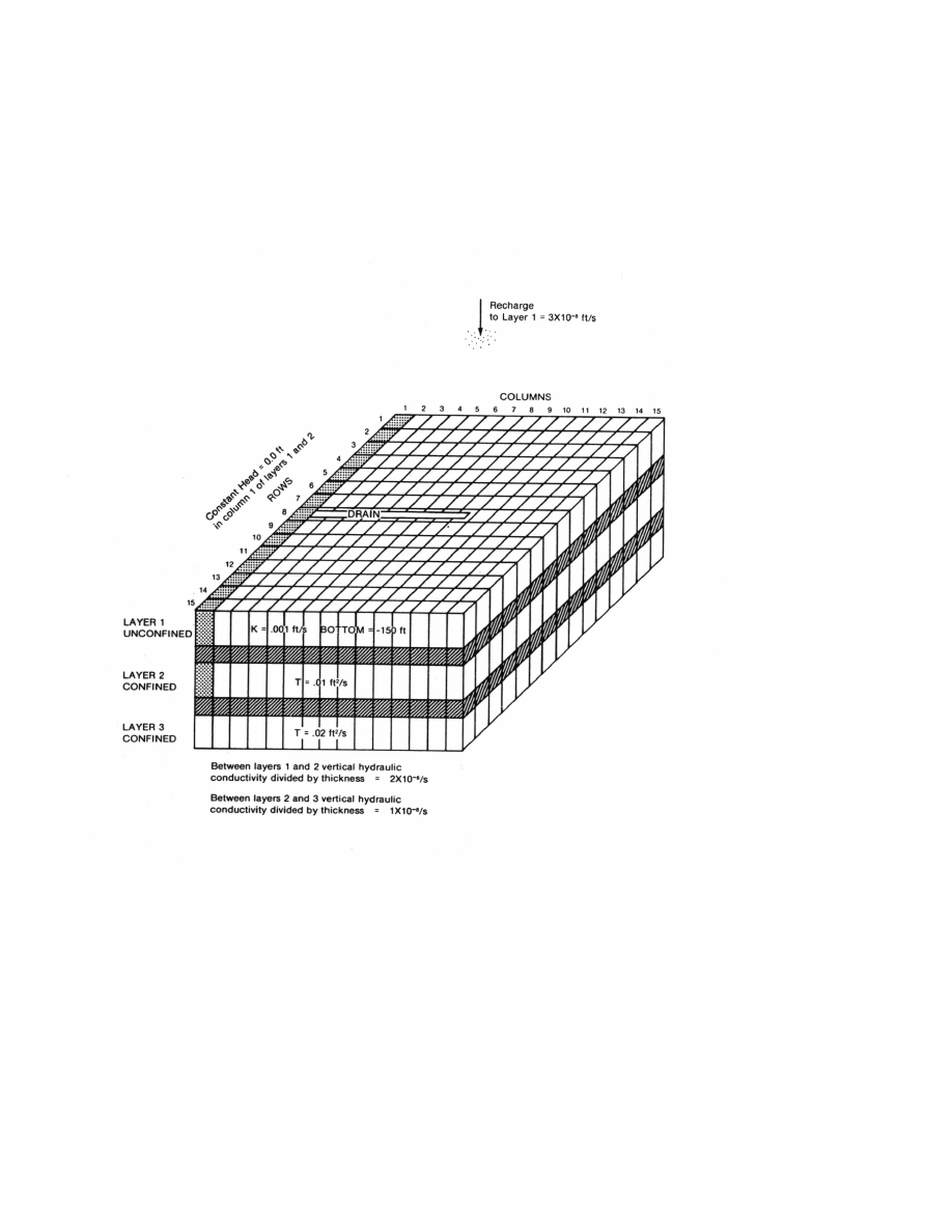
Example

EXAMPLE

The example problem described in McDonald and Harbaugh (1988) and duplicated in Harbaugh and

McDonald (1996a) is used here to demonstrate the use of MODFLOW-2000. The example is implemented two
ways—with and without parameters. For the implementation without parameters, the BCF Package is used as in
McDonald and Harbaugh (1988). When the example is implemented using parameters, the LPF Package is used.
The simulated system is shown in figure 10 (McDonald and Harbaugh, 1988, Appendix D).

Figure 10. -- Illustration of the system simulated in the example problem.

Example Without Parameters

To run the problem without parameters, the example input data from Harbaugh and McDonald (1996a) was

converted by the conversion program described earlier, MF96TO2K. The conversion program requires the user to
specify which model layers are underlain by Quasi-3D confining beds and any elevation data that are not included
in the BCF Package input file. For this problem, the following elevation information must be provided to the
conversion program:

MODFLOW-2000—User Guide to Modularization Concepts and the

Ground-Water Flow Process

•

the elevation of the top of layer 1,

•

the elevations of the bottoms of the confining beds under layers 1 and 2, and

•

the elevations of the bottoms of model layers 2 and 3.

As shown in figure 10, all the layers are flat, but there are no elevations specified except for the bottom of

layer 1. The other elevations were not specified in the original problem because they were not needed in earlier
versions of MODFLOW. Layer thickness is incorporated into transmissivity and vertical leakance (VCONT)
values. For MODFLOW-2000, however, all of the elevations must be specified. Any physically consistent
elevations can be used if the only goal is to reproduce the heads calculated by MODFLOW-96. That is, each
successive layer must have a lower elevation than the layer above, and the top elevation of layer 1 must be above
the water table. Within these constraints, the following values were arbitrarily selected:

Elevation of the top of layer 1 = 200 ft,

Elevation of the bottom of the confining bed below layer 1 = -200 ft,

Elevation of the bottom of layer 2 = -300 ft,

Elevation of the bottom of the confining bed below layer 2 = -350 ft, and

Elevation of the bottom of layer 3 = -450 ft.

The following are the resulting input files:

Name File:

LIST 6 twri.lst

BAS6 5 TWRI.ba6

BCF6 11 TWRI.bc6

WEL 12 twri.wel

DRN 13 twri.drn

RCH 18 twri.rch

SIP 19 twri.sip

OC 22 twri.oc

DIS 10 TWRI.dis

Discretization (DIS) File

3 15 15 1 1 0 NLAY,NROW,NCOL,NPER,ITMUNI,LENUNI

1 1 0

CONSTANT 5.000000E+03 DELR

CONSTANT 5.000000E+03 DELC

CONSTANT 2.000000E+02 TOP of system

CONSTANT -1.500000E+02 Layer BOTM layer 1

CONSTANT -2.000000E+02 Confining bed BOTM layer 1

CONSTANT -3.000000E+02 Layer BOTM layer 2

CONSTANT -3.500000E+02 Confining bed BOTM layer 2

CONSTANT -4.500000E+02 Layer BOTM layer 3

8.640E+04 1 1.000E+00 SS PERLEN,NSTP,TSMULT,Ss/tr

Example

Basic Package (BAS6) File

#SAMPLE---3 LAYERS, 15 ROWS, 15 COLUMNS; STEADY STATE; CONSTANT HEADS COLUMN 1

#LAYERS 1 AND 2; RECHARGE, WELLS AND DRAINS

NO OPTIONS

INTERNAL 1 (20I4) 3 IBOUND layer 1

-1 1 1 1 1 1 1 1 1 1 1 1 1 1 1

INTERNAL 1 (20I4) 3 IBOUND layer 2

-1 1 1 1 1 1 1 1 1 1 1 1 1 1 1

CONSTANT 1 IBOUND layer 3

999.99 HNOFLO

CONSTANT 0.000000E+00 Initial Head layer 1

CONSTANT 0.000000E+00 Initial Head layer 2

CONSTANT 0.000000E+00 Initial Head layer 3

Output Control Option (OC) File—Default output control was used when this problem was run by McDonald

and Harbaugh (1988), so no file was required. The Output Control Option is used here only for the purpose of
changing the format for printing head. A format has been chosen that uses less page width.

HEAD PRINT FORMAT 20

PERIOD 1 STEP 1

PRINT HEAD

MODFLOW-2000—User Guide to Modularization Concepts and the

Ground-Water Flow Process

Block-Centered Flow Package (BCF6) File

0 1.00E+30 0 0.00E+00 0 0

1 0 0

CONSTANT 1.000000E+00 TRPY

CONSTANT 1.000000E-03 HY layer 1

CONSTANT 2.000000E-08 VCONT layer 1

CONSTANT 1.000000E-02 TRAN layer 2

CONSTANT 1.000000E-08 VCONT layer 2

CONSTANT 2.000000E-02 TRAN layer 3

Recharge Package (RCH) File

1 0 NRCHOP,IRCHBD

1 INRECH

0 3.E-8

RECH-1

Well Package (WEL) File

15 0 MXACTW,IWELCB

15 ITMP

3 5 11 -5.

2 4 6 -5.

2 6 12 -5.

1 9 8 -5.

1 9 10 -5.

1 9 12 -5.

1 9 14 -5.

1 11 8 -5.

1 11 10 -5.

1 11 12 -5.

1 11 14 -5.

1 13 8 -5.

1 13 10 -5.

1 13 12 -5.

1 13 14 -5.

Drain Package (DRN) File

9 0 MXACTD,IDRNCB

9 ITMP

1 8 2 0. 1.E00

1 8 3 0. 1.E00

1 8 4 10. 1.E00

1 8 5 20. 1.E00

1 8 6 30. 1.E00

1 8 7 50. 1.E00

1 8 8 70. 1.E00

1 8 9 90. 1.E00

1 8 10 100. 1.E00

Example

Strongly Implicit Procedure Package (SIP) File

50 5 MXITER,NPARM

1. .001 0 .001 1

This problem was run on a personal computer using a runfile that was compiled using the Lahey Fortran 95

compiler. The Name File includes only a LIST output file (i.e., there is no GLOBAL file), so all of the “printed”
output is in a single file. The contents of the LIST file are shown in figure 11.

MODFLOW-2000

U.S. GEOLOGICAL SURVEY MODULAR FINITE-DIFFERENCE GROUND-WATER FLOW MODEL

VERSION 1.00 06/13/2000

This model run combines GLOBAL and LIST output into this single file.

GLOBAL LISTING FILE: twri.lst

UNIT 6

OPENING TWRI.ba6

FILE TYPE:BAS6 UNIT 5

OPENING TWRI.bc6

FILE TYPE:BCF6 UNIT 11

OPENING twri.wel

FILE TYPE:WEL UNIT 12

OPENING twri.drn

FILE TYPE:DRN UNIT 13

OPENING twri.rch

FILE TYPE:RCH UNIT 18

OPENING twri.sip

FILE TYPE:SIP UNIT 19

OPENING twri.oc

FILE TYPE:OC UNIT 22

OPENING TWRI.dis

FILE TYPE:DIS UNIT 10

DISCRETIZATION INPUT DATA READ FROM UNIT 10

3 LAYERS 15 ROWS 15 COLUMNS

1 STRESS PERIOD(S) IN SIMULATION

MODEL TIME UNIT IS SECONDS

MODEL LENGTH UNIT IS UNDEFINED

Figure 11. -- LIST file for example problem without parameters.

MODFLOW-2000—User Guide to Modularization Concepts and the

Ground-Water Flow Process

THE OBSERVATION PROCESS IS INACTIVE

THE SENSITIVITY PROCESS IS INACTIVE

THE PARAMETER-ESTIMATION PROCESS IS INACTIVE

MODE: FORWARD

Confining bed flag for each layer:

1 1 0

6555 ELEMENTS OF GX ARRAY USED OUT OF 6555

675 ELEMENTS OF GZ ARRAY USED OUT OF 675

675 ELEMENTS OF IG ARRAY USED OUT OF 675

DELR = 5000.00

DELC = 5000.00

TOP ELEVATION OF LAYER 1 = 200.000

MODEL LAYER BOTTOM EL. = -150.000 FOR LAYER 1

BOT. EL. OF QUASI-3D BED = -200.000 FOR LAYER 1

MODEL LAYER BOTTOM EL. = -300.000 FOR LAYER 2

BOT. EL. OF QUASI-3D BED = -350.000 FOR LAYER 2

MODEL LAYER BOTTOM EL. = -450.000 FOR LAYER 3

STRESS PERIOD LENGTH TIME STEPS MULTIPLIER FOR DELT SS FLAG

----------------------------------------------------------------------------

1 86400.00 1 1.000 SS

STEADY-STATE SIMULATION

SIP5 -- STRONGLY IMPLICIT PROCEDURE SOLUTION PACKAGE

VERSION 5, 9/1/93 INPUT READ FROM UNIT 19

MAXIMUM OF 50 ITERATIONS ALLOWED FOR CLOSURE

5 ITERATION PARAMETERS

2755 ELEMENTS IN X ARRAY ARE USED BY SIP

150 ELEMENTS IN IX ARRAY ARE USED BY SIP

2755 ELEMENTS OF X ARRAY USED OUT OF 2755

0 ELEMENTS OF Z ARRAY USED OUT OF 1

150 ELEMENTS OF IX ARRAY USED OUT OF 150

0 ELEMENTS OF XHS ARRAY USED OUT OF 1

Figure 11. -- LIST file for example problem without parameters—Continued.

Example

SOLUTION BY THE STRONGLY IMPLICIT PROCEDURE

-------------------------------------------

MAXIMUM ITERATIONS ALLOWED FOR CLOSURE = 50

ACCELERATION PARAMETER = 1.0000

HEAD CHANGE CRITERION FOR CLOSURE = 0.10000E-02

SIP HEAD CHANGE PRINTOUT INTERVAL = 1

5 ITERATION PARAMETERS CALCULATED FROM SPECIFIED WSEED = 0.00100000 :

0.000000E+00 0.822172E+00 0.968377E+00 0.994377E+00 0.999000E+00

#SAMPLE----3 LAYERS, 15 ROWS, 15 COLUMNS; STEADY STATE; CONSTANT HEADS COLUMN 1

#LAYERS 1 AND 2; RECHARGE, WELLS AND DRAINS

3 LAYERS 15 ROWS 15 COLUMNS

1 STRESS PERIOD(S) IN SIMULATION

BAS6 -- BASIC PACKAGE, VERSION 6, 1/11/2000 INPUT READ FROM UNIT 5

15 ELEMENTS IN IR ARRAY ARE USED BY BAS

BCF6 -- BLOCK-CENTERED FLOW PACKAGE, VERSION 6, 1/11/2000

INPUT READ FROM UNIT 11

STEADY-STATE SIMULATION

HEAD AT CELLS THAT CONVERT TO DRY= 0.10000E+31

WETTING CAPABILITY IS NOT ACTIVE

LAYER LAYER-TYPE CODE INTERBLOCK T

--------------------------------------------

1 1 0 -- HARMONIC

2 0 0 -- HARMONIC

3 0 0 -- HARMONIC

678 ELEMENTS IN RX ARRAY ARE USED BY BCF

WEL6 -- WELL PACKAGE, VERSION 6, 1/11/2000 INPUT READ FROM UNIT 12

No named parameters

MAXIMUM OF 15 ACTIVE WELLS AT ONE TIME

60 ELEMENTS IN RX ARRAY ARE USED BY WEL

DRN6 -- DRAIN PACKAGE, VERSION 6, 1/11/2000 INPUT READ FROM UNIT 13

No named parameters

MAXIMUM OF 9 ACTIVE DRAINs AT ONE TIME

45 ELEMENTS IN RX ARRAY ARE USED BY DRN

RCH6 -- RECHARGE PACKAGE, VERSION 6, 1/11/2000 INPUT READ FROM UNIT 18

No named parameters

OPTION 1 -- RECHARGE TO TOP LAYER

225 ELEMENTS IN RX ARRAY ARE USED BY RCH

225 ELEMENTS IN IR ARRAY ARE USED BY RCH

1008 ELEMENTS OF RX ARRAY USED OUT OF 1008

240 ELEMENTS OF IR ARRAY USED OUT OF 240

#SAMPLE----3 LAYERS, 15 ROWS, 15 COLUMNS; STEADY STATE; CONSTANT HEADS COLUMN 1

#LAYERS 1 AND 2; RECHARGE, WELLS AND DRAINS

Figure 11. -- LIST file for example problem without parameters—Continued.

MODFLOW-2000—User Guide to Modularization Concepts and the

Ground-Water Flow Process

BOUNDARY ARRAY FOR LAYER 1

READING ON UNIT 5 WITH FORMAT: (20I4)

1 2 3 4 5 6 7 8 9 10 11 12 13 14 15

................................................................

1 -1 1 1 1 1 1 1 1 1 1 1 1 1 1 1

2 -1 1 1 1 1 1 1 1 1 1 1 1 1 1 1

3 -1 1 1 1 1 1 1 1 1 1 1 1 1 1 1

4 -1 1 1 1 1 1 1 1 1 1 1 1 1 1 1

5 -1 1 1 1 1 1 1 1 1 1 1 1 1 1 1

6 -1 1 1 1 1 1 1 1 1 1 1 1 1 1 1

7 -1 1 1 1 1 1 1 1 1 1 1 1 1 1 1

8 -1 1 1 1 1 1 1 1 1 1 1 1 1 1 1

9 -1 1 1 1 1 1 1 1 1 1 1 1 1 1 1

10 -1 1 1 1 1 1 1 1 1 1 1 1 1 1 1

11 -1 1 1 1 1 1 1 1 1 1 1 1 1 1 1

12 -1 1 1 1 1 1 1 1 1 1 1 1 1 1 1

13 -1 1 1 1 1 1 1 1 1 1 1 1 1 1 1

14 -1 1 1 1 1 1 1 1 1 1 1 1 1 1 1

15 -1 1 1 1 1 1 1 1 1 1 1 1 1 1 1

BOUNDARY ARRAY FOR LAYER 2

READING ON UNIT 5 WITH FORMAT: (20I4)

1 2 3 4 5 6 7 8 9 10 11 12 13 14 15

................................................................

1 -1 1 1 1 1 1 1 1 1 1 1 1 1 1 1

2 -1 1 1 1 1 1 1 1 1 1 1 1 1 1 1

3 -1 1 1 1 1 1 1 1 1 1 1 1 1 1 1

4 -1 1 1 1 1 1 1 1 1 1 1 1 1 1 1

5 -1 1 1 1 1 1 1 1 1 1 1 1 1 1 1

6 -1 1 1 1 1 1 1 1 1 1 1 1 1 1 1

7 -1 1 1 1 1 1 1 1 1 1 1 1 1 1 1

8 -1 1 1 1 1 1 1 1 1 1 1 1 1 1 1

9 -1 1 1 1 1 1 1 1 1 1 1 1 1 1 1

10 -1 1 1 1 1 1 1 1 1 1 1 1 1 1 1

11 -1 1 1 1 1 1 1 1 1 1 1 1 1 1 1

12 -1 1 1 1 1 1 1 1 1 1 1 1 1 1 1

13 -1 1 1 1 1 1 1 1 1 1 1 1 1 1 1

14 -1 1 1 1 1 1 1 1 1 1 1 1 1 1 1

15 -1 1 1 1 1 1 1 1 1 1 1 1 1 1 1

BOUNDARY ARRAY = 1 FOR LAYER 3

AQUIFER HEAD WILL BE SET TO 999.99 AT ALL NO-FLOW NODES (IBOUND=0).

INITIAL HEAD = 0.000000 FOR LAYER 1

INITIAL HEAD = 0.000000 FOR LAYER 2

INITIAL HEAD = 0.000000 FOR LAYER 3

Figure 11. -- LIST file for example problem without parameters—Continued.

Example

OUTPUT CONTROL IS SPECIFIED ONLY AT TIME STEPS FOR WHICH OUTPUT IS DESIRED

HEAD PRINT FORMAT CODE IS 20 DRAWDOWN PRINT FORMAT CODE IS 0

HEADS WILL BE SAVED ON UNIT 0 DRAWDOWNS WILL BE SAVED ON UNIT 0

COLUMN TO ROW ANISOTROPY = 1.00000

HYD. COND. ALONG ROWS = 1.000000E-03 FOR LAYER 1

VERT HYD COND /THICKNESS = 2.000000E-08 FOR LAYER 1

TRANSMIS. ALONG ROWS = 1.000000E-02 FOR LAYER 2

VERT HYD COND /THICKNESS = 1.000000E-08 FOR LAYER 2

TRANSMIS. ALONG ROWS = 2.000000E-02 FOR LAYER 3

0 Well parameters

0 Drain parameters

0 Recharge parameters

STRESS PERIOD NO. 1, LENGTH = 86400.00

----------------------------------------------

NUMBER OF TIME STEPS = 1

MULTIPLIER FOR DELT = 1.000

INITIAL TIME STEP SIZE = 86400.00

WELL NO. LAYER ROW COL STRESS RATE

--------------------------------------------

1 3 5 11 -5.000

2 2 4 6 -5.000

3 2 6 12 -5.000

4 1 9 8 -5.000

5 1 9 10 -5.000

6 1 9 12 -5.000

7 1 9 14 -5.000

8 1 11 8 -5.000

9 1 11 10 -5.000

10 1 11 12 -5.000

11 1 11 14 -5.000

12 1 13 8 -5.000

13 1 13 10 -5.000

14 1 13 12 -5.000

15 1 13 14 -5.000

15 WELLS

Figure 11. -- LIST file for example problem without parameters—Continued.

MODFLOW-2000—User Guide to Modularization Concepts and the

Ground-Water Flow Process

DRAIN NO. LAYER ROW COL DRAIN EL. CONDUCTANCE

----------------------------------------------------------

1 1 8 2 0.0000 1.000

2 1 8 3 0.0000 1.000

3 1 8 4 10.00 1.000

4 1 8 5 20.00 1.000

5 1 8 6 30.00 1.000

6 1 8 7 50.00 1.000

7 1 8 8 70.00 1.000

8 1 8 9 90.00 1.000

9 1 8 10 100.0 1.000

9 DRAINS

RECHARGE = 3.000000E-08

SOLVING FOR HEAD

31 ITERATIONS FOR TIME STEP 1 IN STRESS PERIOD 1

MAXIMUM HEAD CHANGE FOR EACH ITERATION:

HEAD CHANGE HEAD CHANGE HEAD CHANGE HEAD CHANGE HEAD CHANGE

LAYER,ROW,COL LAYER,ROW,COL LAYER,ROW,COL LAYER,ROW,COL LAYER,ROW,COL

----------------------------------------------------------------------

-22.41 12.48 13.39 48.21 35.91

( 3, 5, 11) ( 1, 1, 15) ( 3, 1, 14) ( 1, 1, 15) ( 3, 1, 13)

2.482 1.430 6.214 7.411 13.66

( 1, 9, 14) ( 3, 10, 13) ( 1, 12, 14) ( 3, 11, 14) ( 1, 15, 15)

0.5503 0.4821 0.4711 2.019 2.302

( 3, 8, 7) ( 2, 6, 9) ( 3, 5, 10) ( 1, 11, 14) ( 3, 5, 13)

0.1108 0.7059E-01 0.2819 0.3141 0.3320

( 1, 13, 12) ( 3, 12, 11) ( 1, 14, 14) ( 3, 13, 14) ( 1, 15, 15)

0.7853E-02 0.1586E-01 0.1777E-01 0.7910E-01 0.8500E-01

( 1, 13, 12) ( 2, 11, 11) ( 3, 11, 10) ( 1, 14, 14) ( 3, 7, 14)

0.4169E-02 0.2555E-02 0.9769E-02 0.1082E-01 0.1030E-01

( 1, 13, 14) ( 3, 14, 15) ( 1, 14, 14) ( 3, 13, 14) ( 1, 15, 15)

0.2430E-03

( 1, 13, 12)

OUTPUT CONTROL FOR STRESS PERIOD 1 TIME STEP 1

PRINT HEAD FOR ALL LAYERS

HEAD IN LAYER 1 AT END OF TIME STEP 1 IN STRESS PERIOD 1

-----------------------------------------------------------------------

1 2 3 4 5 6

7 8 9 10 11 12

13 14 15

........................................................................

1 0.0000 24.94 44.01 59.26 71.82 82.52

91.91 100.0 106.9 112.6 117.4 121.3

124.3 126.4 127.4

Figure 11. -- LIST file for example problem without parameters—Continued.

Example

2 0.0000 24.45 43.10 57.98 70.17 80.57

90.12 98.40 105.3 111.0 115.7 119.6

122.7 124.9 126.1

3 0.0000 23.45 41.30 55.43 66.78 76.21

86.51 95.20 102.2 107.6 112.0 116.1

119.6 122.1 123.4

4 0.0000 21.92 38.61 51.75 61.79 68.03

81.34 90.75 97.64 102.5 106.1 110.7

114.9 117.9 119.4

5 0.0000 19.73 34.92 47.32 57.69 66.74

77.09 85.76 92.22 96.15 97.29 103.1

108.8 112.5 114.3

6 0.0000 16.51 29.50 40.90 51.30 61.21

71.19 79.85 86.47 90.82 93.03 94.23

102.1 106.4 108.4

7 0.0000 11.55 21.10 31.21 41.40 51.84

63.08 72.68 79.95 84.92 88.60 91.66

96.43 99.82 101.8

8 0.0000 3.483 6.832 16.25 26.30 36.97

52.59 64.31 72.52 77.25 81.99 85.00

89.27 91.72 94.33

9 0.0000 10.54 19.11 28.12 36.92 45.27

52.95 55.38 65.15 66.07 73.93 73.79

80.84 80.17 86.49

10 0.0000 14.62 25.86 35.38 43.49 50.11

54.93 57.55 62.95 65.55 70.39 72.44

76.72 78.26 81.79

11 0.0000 17.11 29.96 40.01 47.78 53.24

55.81 53.33 60.27 59.29 66.43 65.45

72.22 71.04 77.62

12 0.0000 18.68 32.56 43.07 50.81 55.92

58.33 58.47 61.93 63.18 67.12 68.50

72.29 73.46 76.85

13 0.0000 19.67 34.24 45.14 53.01 58.04

59.91 56.75 62.59 60.91 67.22 65.75

71.90 70.35 76.48

14 0.0000 20.27 35.27 46.48 54.61 60.08

63.17 64.52 67.25 68.79 71.64 73.18

75.84 77.03 79.09

15 0.0000 20.56 35.78 47.16 55.48 61.26

65.02 67.52 69.94 72.01 74.29 76.22

78.22 79.66 80.82

HEAD IN LAYER 2 AT END OF TIME STEP 1 IN STRESS PERIOD 1

-----------------------------------------------------------------------

1 2 3 4 5 6

7 8 9 10 11 12

13 14 15

........................................................................

1 0.0000 24.66 43.73 59.02 71.61 82.32

91.72 99.86 106.7 112.5 117.2 121.1

124.1 126.2 127.3

Figure 11. -- LIST file for example problem without parameters—Continued.

MODFLOW-2000—User Guide to Modularization Concepts and the

Ground-Water Flow Process

100

2 0.0000 24.17 42.83 57.74 69.95 80.36

89.93 98.22 105.1 110.8 115.5 119.4

122.6 124.8 125.9

3 0.0000 23.17 41.03 55.19 66.53 75.77

86.29 95.02 102.0 107.4 111.8 116.0

119.5 121.9 123.2

4 0.0000 21.65 38.34 51.50 61.35 60.17

80.90 90.55 97.45 102.3 105.4 110.4

114.8 117.7 119.2

5 0.0000 19.48 34.65 47.07 57.44 66.30

76.85 85.57 92.00 95.41 91.09 102.1

108.6 112.4 114.2

6 0.0000 16.27 29.24 40.65 51.07 60.98

70.98 79.65 86.28 90.54 92.06 86.23

101.7 106.2 108.3

7 0.0000 11.38 20.95 31.05 41.25 51.70

62.90 72.48 79.76 84.73 88.35 91.24

96.22 99.65 101.6

8 0.0000 4.209 8.330 17.58 27.58 38.25

52.94 64.19 72.34 77.12 81.81 84.86

89.10 91.59 94.17

9 0.0000 10.38 18.96 27.98 36.79 45.16

52.86 56.13 65.08 66.79 73.87 74.48

80.77 80.84 86.38

10 0.0000 14.40 25.61 35.15 43.27 49.91

54.76 57.48 62.79 65.49 70.24 72.37

76.57 78.20 81.64

11 0.0000 16.87 29.70 39.78 47.56 53.05

55.68 54.09 60.20 60.04 66.37 66.18

72.16 71.75 77.51

12 0.0000 18.43 32.31 42.85 50.60 55.73

58.16 58.41 61.78 63.12 66.98 68.44

72.15 73.40 76.69

13 0.0000 19.42 33.98 44.91 52.80 57.85

59.78 57.50 62.53 61.65 67.16 66.48

71.84 71.06 76.37

14 0.0000 20.02 35.02 46.26 54.41 59.88

62.99 64.39 67.08 68.66 71.48 73.06

75.68 76.91 78.93

15 0.0000 20.30 35.52 46.94 55.28 61.07

64.84 67.34 69.76 71.84 74.11 76.04

78.04 79.49 80.65

HEAD IN LAYER 3 AT END OF TIME STEP 1 IN STRESS PERIOD 1

-----------------------------------------------------------------------

1 2 3 4 5 6

7 8 9 10 11 12

13 14 15

........................................................................

1 1.800 24.34 43.36 58.70 71.33 82.06

91.48 99.63 106.5 112.3 117.0 120.9

123.9 126.0 127.1

Figure 11. -- LIST file for example problem without parameters—Continued.

Example

101

2 1.764 23.85 42.46 57.42 69.66 80.07

89.68 97.99 104.9 110.6 115.3 119.2

122.4 124.6 125.7

3 1.691 22.86 40.67 54.87 66.20 75.28

85.98 94.77 101.7 107.2 111.5 115.7

119.3 121.7 123.0

4 1.578 21.35 37.98 51.17 60.85 62.69

80.41 90.28 97.19 101.9 104.1 110.0

114.5 117.5 119.0

5 1.415 19.18 34.30 46.75 57.10 65.80

76.54 85.30 91.67 94.17 77.46 100.7

108.2 112.1 114.0

6 1.176 15.99 28.91 40.33 50.76 60.67

70.70 79.38 86.01 90.12 90.60 88.55

101.2 106.0 108.0

7 0.8273 11.21 20.79 30.88 41.09 51.55

62.67 72.22 79.50 84.46 87.98 90.77

95.94 99.41 101.4

8 0.4331 5.131 10.19 19.27 29.19 39.84

53.40 64.07 72.11 76.95 81.58 84.68

88.88 91.44 93.95

9 0.7543 10.22 18.82 27.84 36.66 45.06

52.78 57.03 65.02 67.64 73.81 75.31

80.72 81.64 86.24

10 1.039 14.13 25.29 34.85 42.99 49.65

54.54 57.44 62.61 65.44 70.05 72.33

76.39 78.15 81.43

11 1.224 16.59 29.37 39.47 47.28 52.79

55.53 55.01 60.16 60.94 66.33 67.06

72.13 72.60 77.38

12 1.341 18.15 31.97 42.54 50.32 55.47

57.94 58.37 61.60 63.08 66.80 68.41

71.97 73.36 76.49

13 1.415 19.14 33.65 44.61 52.53 57.60

59.63 58.39 62.48 62.54 67.12 67.35

71.80 71.90 76.24

14 1.460 19.73 34.68 45.96 54.13 59.63

62.76 64.24 66.87 68.52 71.27 72.91

75.47 76.77 78.71

15 1.481 20.01 35.18 46.63 55.00 60.81

64.59 67.11 69.52 71.61 73.87 75.82

77.81 79.27 80.42

VOLUMETRIC BUDGET FOR ENTIRE MODEL AT END OF TIME STEP 1 IN STRESS PERIOD 1

-----------------------------------------------------------------------------

CUMULATIVE VOLUMES L**3 RATES FOR THIS TIME STEP L**3/T

------------------ ------------------------

Figure 11. -- LIST file for example problem without parameters—Continued.

MODFLOW-2000—User Guide to Modularization Concepts and the

Ground-Water Flow Process

102

IN: IN:

--- ---

STORAGE = 0.0000 STORAGE = 0.0000

CONSTANT HEAD = 0.0000 CONSTANT HEAD = 0.0000

WELLS = 0.0000 WELLS = 0.0000

DRAINS = 0.0000 DRAINS = 0.0000

RECHARGE = 13608000.0000 RECHARGE = 157.5000

TOTAL IN = 13608000.0000 TOTAL IN = 157.5000

OUT: OUT:

---- ----

STORAGE = 0.0000 STORAGE = 0.0000

CONSTANT HEAD = 4326522.5000 CONSTANT HEAD = 50.0755

WELLS = 6480000.0000 WELLS = 75.0000

DRAINS = 2801081.2500 DRAINS = 32.4199

RECHARGE = 0.0000 RECHARGE = 0.0000

TOTAL OUT = 13607603.0000 TOTAL OUT = 157.4954

IN - OUT = 397.0000 IN - OUT = 4.5929E-03

PERCENT DISCREPANCY = 0.00 PERCENT DISCREPANCY = 0.00

TIME SUMMARY AT END OF TIME STEP 1 IN STRESS PERIOD 1

SECONDS MINUTES HOURS DAYS YEARS

-----------------------------------------------------------

TIME STEP LENGTH 86400. 1440.0 24.000 1.0000 2.73785E-03

STRESS PERIOD TIME 86400. 1440.0 24.000 1.0000 2.73785E-03

TOTAL TIME 86400. 1440.0 24.000 1.0000 2.73785E-03

Figure 11. -- LIST file for example problem without parameters—Continued.

Example With Parameters

The same problem is repeated using the LPF Package. LPF does not have an option to enter transmissivity

for confined layers; instead, horizontal hydraulic conductivity (HK) must be entered for all layers. HK values for
layers 2 and 3 were not directly specified in the problem, but HK can be easily calculated from the specified
values of transmissivity and the assumed layer thicknesses.

LPF also differs from BCF in the way vertical hydraulic information is entered. LPF requires vertical

hydraulic conductivity information for each model layer and Quasi-3D confining bed, whereas BCF requires only
the vertical leakance (VCONT) between nodes, which is the average vertical hydraulic conductivity (including a
Quasi-3D confining bed if it exists) divided by the distance between nodes. The BCF user must calculate a
representative VCONT from the VCONT of three individual components. For example, for a cell in layer 1,
VCONT is calculated from the VCONT of half the thickness of layer 1, the full thickness of the confining bed,
and half the thickness of layer 2 (McDonald and Harbaugh, 1988, p. 5-16). There is no unique way to calculate
the vertical hydraulic conductivity of each layer based on the BCF VCONT values, which is all that the original

Example

103

problem specified. The approach used here is to assume that the confining bed dominates the VCONT calculation
and that there is virtually no contribution from the actual model layers, which is consistent with the assumptions
used in making the Quasi-3D approximation. If the model layers have no influence on VCONT, then VKCB is
VCONT times the confining-bed thickness. For layer 1, VKCB is 10

-6

ft/s; for layer 2 it is 5x10

-7

ft/s.

Although it is assumed for the above calculation of VKCB that there is no contribution to CV from the

aquifer vertical hydraulic conductivity (VK), LPF requires VK to be specified as part of the input data. According
to equation 27, VK should be infinite in order to have no impact on CV. There is no way to directly specify an
infinite value for VK, but the effect of having an infinite value can be obtained by making the VK values large
compared to VKCB. For this example problem, VK is set to 1.0 ft/s for all model layers, which is a million times
larger than the largest VKCB. The low impact of this value on CV is demonstrated by the fact that the calculated
head as shown in the LIST file when LPF is used (fig. 13) is the same as the head in the BCF LIST file (fig. 11).

Note that any combination of VK and CBVK that produces virtually the same CV that BCF calculates using

the original VCONT values will produce the same heads in this problem. If the values of VK for layer 1 were
relatively small compared to CBVK, then the VK values would have to be varied from cell to cell due to the fact
that the saturated thickness of layer 1 varies; that is, as indicated by equation 27, the conductance between cells
depends on saturated thickness of the model cells. Thus, the choice to use a large VK in order to essentially
eliminate the aquifer contribution to CV makes the LPF input simpler than it would otherwise be.

Another difference in the input data for this problem is that parameters are used for defining some of the data

in order to illustrate the use of parameters. Parameters are used for defining HK, VKCB, RECH, WELL, and
DRAI input variables. In the LPF Package, five parameters are used—three define HK, and two define VKCB.
Each of these parameters is for a single layer, and each parameter has a uniform value for the entire layer. HK1,
HK2, and HK3 are HK for layers 1, 2, and 3, respectively. These use “NONE” for the multiplier array, which
means that there is no multiplier array. Instead, the parameter value applies directly to all of the included cells.
The zone array is “ALL”, which means the values for all cells in the indicated layer are defined by the parameter.
Parameter VKCB1 defines VKCB values for all of layer 1, and VKCB2 defines VKCB values for layer 2. Both of
these parameters use the same multiplier array, which has a value of 1.0E-6 at all cells. The parameter value for
VKCB1 is 1.0, and the value for VKCB2 is 0.5, which produces the required values of 1.0E-6 for layer 1 and
5.0E-7 for layer 2.

For the RCH Package, two parameters, RCH1 and RCH2, are used. RCH1 includes the left seven columns of

the grid, and RCH2 includes the right 8 columns. These areas are specified using zone array RCHZONES.
RCHZONES contains “1” in columns 1-7, and “2” in columns 8-15. Accordingly, the zone value of 1 is specified
in the definition of RCH1, and zone value 2 is specified for RCH2. The parameter values for RCH1 and RCH2
are both 3.0E-8, which results in all cells having the same recharge rate. Thus, there is no advantage of having
two parameters in this example; however, two zones were used to illustrate how this is done. The value of having
two zones would become apparent if there were a need to change the recharge rate in the area of zone 1 without
changing the zone 2 values. This could be done simply by changing the value of parameter RCH1.

The Well Package has one parameter, WELL1, and the Drain Package has one parameter, DRN1. Both of

these parameters have a value of 1.0, so the multipliers in the lists for both parameters are simply the same as the
data values that are used to define the input data without using parameters. There could be an advantage of using
parameters, however, if there were a need to change all of the input values associated with the parameters. All of
the values could be changed by a constant factor simply by changing the parameter values. The parameters define
only part of the wells and drains. Some of them are defined as separate non-parameter lists.

The input files that are different as a result of using LPF instead of BCF and adding parameters are shown

below. The DIS, BAS, SIP, and OC files are not shown again because they are unchanged.

Name File

GLOBAL 1 twri.glo

LIST 6 twri.lst

BAS6 5 TWRI.ba6

MODFLOW-2000—User Guide to Modularization Concepts and the

Ground-Water Flow Process

104

LPF 11 twri.lpf

WEL 12 twri.wel

DRN 13 twri.drn

RCH 18 twri.rch

SIP 19 twri.sip

OC 22 twri.oc

MULT 8 twri.mlt

ZONE 9 twri.zon

DIS 10 TWRI.dis

Multiplier File

MULT1

CONSTANT 1.0E-6

Zone File

RCHZONES

INTERNAL 1 (15I2) 1

1 1 1 1 1 1 1 2 2 2 2 2 2 2 2

Layer-Property Flow Package (LPF) File

# LPF Package input data for example problem

0 1.00E+30 5 ILPFCB,HDRY,NPLPF

1 0 0

0 0 0

1. 1. 1.

0 0 0

Example

105

0 0 0

HK1 HK 1.0E-3 1

1 NONE ALL

HK2 HK 1.0E-4 1

2 NONE ALL

HK3 HK 2.0E-4 1

3 NONE ALL

VKCB1 VKCB 1.0 1

1 MULT1 ALL

VKCB2 VKCB 0.5 1

2 MULT1 ALL

0 HK layer 1

CONSTANT 1.0 VK layer 1

0 VKCB layer 1

0 HK layer 2

CONSTANT 1.0 VK layer 2

0 VKCB layer 2

0 HK ayer 3

CONSTANT 1.0 VK layer 3

Recharge Package (RCH) File

PARAMETER 2

1 0 NRCHOP,IRCHBD

RCH1 RCH 3.0E-8 1

NONE RCHZONES 1

RCH2 RCH 3.0E-8 1

NONE RCHZONES 2

2 INRECH

RCH1

RCH2

Well Package (WEL) File

PARAMETER 1 12

15 0 MXACTW,IWELCB

WELL1 Q 1.0 12

1 9 8 -5.

1 9 10 -5.

1 9 12 -5.

1 9 14 -5.

1 11 8 -5.

1 11 10 -5.

1 11 12 -5.

1 11 14 -5.

MODFLOW-2000—User Guide to Modularization Concepts and the

Ground-Water Flow Process

106

1 13 8 -5.

1 13 10 -5.

1 13 12 -5.

1 13 14 -5.

3 1 ITMP,NP

3 5 11 -5.

2 4 6 -5.

2 6 12 -5.

WELL1

Drain Package (DRN) File

PARAMETER 1 2

9 0 MXACTD,IDRNCB

DRN1 DRN 1.0 2

1 8 2 0. 1.E00

1 8 3 0. 1.E00

7 1 ITMP,NP

1 8 4 10. 1.E00

1 8 5 20. 1.E00

1 8 6 30. 1.E00

1 8 7 50. 1.E00

1 8 8 70. 1.E00

1 8 9 90. 1.E00

1 8 10 100. 1.E00

DRN1

The Name File specifies both GLOBAL and LIST output files. The GLOBAL file is shown in figure 12, and

the LIST file is shown in figure 13.

Example

107

MODFLOW-2000

U.S. GEOLOGICAL SURVEY MODULAR FINITE-DIFFERENCE GROUND-WATER FLOW MODEL

VERSION 1.00 06/13/2000

This model run produced both GLOBAL and LIST files. This is the GLOBAL file.

GLOBAL LISTING FILE: twri.glo

UNIT 1

OPENING twri.lst

FILE TYPE:LIST UNIT 6

OPENING TWRI.ba6

FILE TYPE:BAS6 UNIT 5

OPENING twri.lpf

FILE TYPE:LPF UNIT 11

OPENING twri.wel

FILE TYPE:WEL UNIT 12

OPENING twri.drn

FILE TYPE:DRN UNIT 13

OPENING twri.rch

FILE TYPE:RCH UNIT 18

OPENING twri.sip

FILE TYPE:SIP UNIT 19

OPENING twri.oc

FILE TYPE:OC UNIT 22

OPENING twri.mlt

FILE TYPE:MULT UNIT 8

OPENING twri.zon

FILE TYPE:ZONE UNIT 9

OPENING TWRI.dis

FILE TYPE:DIS UNIT 10

DISCRETIZATION INPUT DATA READ FROM UNIT 10

3 LAYERS 15 ROWS 15 COLUMNS

1 STRESS PERIOD(S) IN SIMULATION

MODEL TIME UNIT IS SECONDS

MODEL LENGTH UNIT IS UNDEFINED

Figure 12. -- GLOBAL file for example problem with parameters.

MODFLOW-2000—User Guide to Modularization Concepts and the

Ground-Water Flow Process

108

THE OBSERVATION PROCESS IS INACTIVE

THE SENSITIVITY PROCESS IS INACTIVE

THE PARAMETER-ESTIMATION PROCESS IS INACTIVE

MODE: FORWARD

ZONE OPTION, INPUT READ FROM UNIT 9

1 ZONE ARRAYS

MULTIPLIER OPTION, INPUT READ FROM UNIT 8

1 MULTIPLIER ARRAYS

Confining bed flag for each layer:

1 1 0

6780 ELEMENTS OF GX ARRAY USED OUT OF 6780

675 ELEMENTS OF GZ ARRAY USED OUT OF 675

900 ELEMENTS OF IG ARRAY USED OUT OF 900

DELR = 5000.00

DELC = 5000.00

TOP ELEVATION OF LAYER 1 = 200.000

MODEL LAYER BOTTOM EL. = -150.000 FOR LAYER 1

BOT. EL. OF QUASI-3D BED = -200.000 FOR LAYER 1

MODEL LAYER BOTTOM EL. = -300.000 FOR LAYER 2

BOT. EL. OF QUASI-3D BED = -350.000 FOR LAYER 2

MODEL LAYER BOTTOM EL. = -450.000 FOR LAYER 3

STRESS PERIOD LENGTH TIME STEPS MULTIPLIER FOR DELT SS FLAG

----------------------------------------------------------------------------

1 86400.00 1 1.000 SS

STEADY-STATE SIMULATION

MULT. ARRAY: MULT1 = 1.000000E-06

ZONE ARRAY: RCHZONES

READING ON UNIT 9 WITH FORMAT: (15I2)

Figure 12. -- GLOBAL file for example problem with parameters—Continued.

Example

109

1 2 3 4 5 6 7 8 9101112131415

..................................

1 1 1 1 1 1 1 1 2 2 2 2 2 2 2 2

2 1 1 1 1 1 1 1 2 2 2 2 2 2 2 2

3 1 1 1 1 1 1 1 2 2 2 2 2 2 2 2

4 1 1 1 1 1 1 1 2 2 2 2 2 2 2 2

5 1 1 1 1 1 1 1 2 2 2 2 2 2 2 2

6 1 1 1 1 1 1 1 2 2 2 2 2 2 2 2

7 1 1 1 1 1 1 1 2 2 2 2 2 2 2 2

8 1 1 1 1 1 1 1 2 2 2 2 2 2 2 2

9 1 1 1 1 1 1 1 2 2 2 2 2 2 2 2

10 1 1 1 1 1 1 1 2 2 2 2 2 2 2 2

11 1 1 1 1 1 1 1 2 2 2 2 2 2 2 2

12 1 1 1 1 1 1 1 2 2 2 2 2 2 2 2

13 1 1 1 1 1 1 1 2 2 2 2 2 2 2 2

14 1 1 1 1 1 1 1 2 2 2 2 2 2 2 2

15 1 1 1 1 1 1 1 2 2 2 2 2 2 2 2

LPF1 -- LAYER PROPERTY FLOW PACKAGE, VERSION 1, 1/11/2000

INPUT READ FROM UNIT 11

# LPF Package input data for example problem

HEAD AT CELLS THAT CONVERT TO DRY= 1.00000E+30

5 Named Parameters

LAYER FLAGS:

LAYER LAYTYP LAYAVG CHANI LAYVKA LAYWET

---------------------------------------------------------------------------

1 1 0 1.000E+00 0 0

2 0 0 1.000E+00 0 0

3 0 0 1.000E+00 0 0

INTERPRETATION OF LAYER FLAGS:

INTERBLOCK HORIZONTAL DATA IN

LAYER TYPE TRANSMISSIVITY ANISOTROPY ARRAY VKA WETTABILITY

LAYER (LAYTYP) (LAYAVG) (CHANI) (LAYVKA) (LAYWET)

---------------------------------------------------------------------------

1 CONVERTIBLE HARMONIC 1.000E+00 VERTICAL K NON-WETTABLE

2 CONFINED HARMONIC 1.000E+00 VERTICAL K NON-WETTABLE

3 CONFINED HARMONIC 1.000E+00 VERTICAL K NON-WETTABLE

1800 ELEMENTS IN X ARRAY ARE USED BY LPF

18 ELEMENTS IN IX ARRAY ARE USED BY LPF

SIP5 -- STRONGLY IMPLICIT PROCEDURE SOLUTION PACKAGE

VERSION 5, 9/1/93 INPUT READ FROM UNIT 19

MAXIMUM OF 50 ITERATIONS ALLOWED FOR CLOSURE

5 ITERATION PARAMETERS

2755 ELEMENTS IN X ARRAY ARE USED BY SIP

150 ELEMENTS IN IX ARRAY ARE USED BY SIP

Figure 12. -- GLOBAL file for example problem with parameters—Continued.

MODFLOW-2000—User Guide to Modularization Concepts and the

Ground-Water Flow Process

110

4555 ELEMENTS OF X ARRAY USED OUT OF 4555

0 ELEMENTS OF Z ARRAY USED OUT OF 1

168 ELEMENTS OF IX ARRAY USED OUT OF 168

0 ELEMENTS OF XHS ARRAY USED OUT OF 1

SOLUTION BY THE STRONGLY IMPLICIT PROCEDURE

-------------------------------------------

MAXIMUM ITERATIONS ALLOWED FOR CLOSURE = 50

ACCELERATION PARAMETER = 1.0000

HEAD CHANGE CRITERION FOR CLOSURE = 0.10000E-02

SIP HEAD CHANGE PRINTOUT INTERVAL = 1

5 ITERATION PARAMETERS CALCULATED FROM SPECIFIED WSEED = 0.00100000 :

0.000000E+00 0.822172E+00 0.968377E+00 0.994377E+00 0.999000E+00

WETTING CAPABILITY IS NOT ACTIVE IN ANY LAYER

PARAMETERS DEFINED IN THE LPF PACKAGE

PARAMETER NAME:HK1 TYPE:HK CLUSTERS: 1

Parameter value from package file is: 1.00000E-03

LAYER: 1 MULTIPLIER ARRAY: NONE ZONE ARRAY: ALL

PARAMETER NAME:HK2 TYPE:HK CLUSTERS: 1

Parameter value from package file is: 1.00000E-04

LAYER: 2 MULTIPLIER ARRAY: NONE ZONE ARRAY: ALL

PARAMETER NAME:HK3 TYPE:HK CLUSTERS: 1

Parameter value from package file is: 2.00000E-04

LAYER: 3 MULTIPLIER ARRAY: NONE ZONE ARRAY: ALL

PARAMETER NAME:VKCB1 TYPE:VKCB CLUSTERS: 1

Parameter value from package file is: 1.0000

LAYER: 1 MULTIPLIER ARRAY: MULT1 ZONE ARRAY: ALL

PARAMETER NAME:VKCB2 TYPE:VKCB CLUSTERS: 1

Parameter value from package file is: 0.50000

LAYER: 2 MULTIPLIER ARRAY: MULT1 ZONE ARRAY: ALL

HYD. COND. ALONG ROWS FOR LAYER 1 WILL BE DEFINED BY PARAMETERS

(PRINT FLAG= 0)

VERTICAL HYD. COND. = 1.00000 FOR LAYER 1

QUASI3D VERT. HYD. COND. FOR LAYER 1 WILL BE DEFINED BY PARAMETERS

(PRINT FLAG= 0)

HYD. COND. ALONG ROWS FOR LAYER 2 WILL BE DEFINED BY PARAMETERS

(PRINT FLAG= 0)

Figure 12. -- GLOBAL file for example problem with parameters—Continued.

Example

111

VERTICAL HYD. COND. = 1.00000 FOR LAYER 2

QUASI3D VERT. HYD. COND. FOR LAYER 2 WILL BE DEFINED BY PARAMETERS

(PRINT FLAG= 0)

HYD. COND. ALONG ROWS FOR LAYER 3 WILL BE DEFINED BY PARAMETERS

(PRINT FLAG= 0)

VERTICAL HYD. COND. = 1.00000 FOR LAYER 3

1 Well parameters

PARAMETER NAME:WELL1 TYPE:Q

Parameter value from package file is: 1.0000

NUMBER OF ENTRIES: 12

WELL NO. LAYER ROW COL STRESS FACTOR

----------------------------------------------

1 1 9 8 -5.000

2 1 9 10 -5.000

3 1 9 12 -5.000

4 1 9 14 -5.000

5 1 11 8 -5.000

6 1 11 10 -5.000

7 1 11 12 -5.000

8 1 11 14 -5.000

9 1 13 8 -5.000

10 1 13 10 -5.000

11 1 13 12 -5.000

12 1 13 14 -5.000

1 Drain parameters

PARAMETER NAME:DRN1 TYPE:DRN

Parameter value from package file is: 1.0000

NUMBER OF ENTRIES: 2

DRAIN NO. LAYER ROW COL DRAIN EL. STRESS FACTOR

------------------------------------------------------------

1 1 8 2 0.0000 1.000

2 1 8 3 0.0000 1.000

2 Recharge parameters

PARAMETER NAME:RCH1 TYPE:RCH CLUSTERS: 1

Parameter value from package file is: 3.00000E-08

MULTIPLIER ARRAY: NONE ZONE ARRAY: RCHZONES

ZONE VALUES: 1

Figure 12. -- GLOBAL file for example problem with parameters—Continued.

MODFLOW-2000—User Guide to Modularization Concepts and the

Ground-Water Flow Process

112

PARAMETER NAME:RCH2 TYPE:RCH CLUSTERS: 1

Parameter value from package file is: 3.00000E-08

MULTIPLIER ARRAY: NONE ZONE ARRAY: RCHZONES

ZONE VALUES: 2

9 PARAMETERS HAVE BEEN DEFINED IN ALL PACKAGES.

(SPACE IS ALLOCATED FOR 500 PARAMETERS.)

Figure 12. -- GLOBAL file for example problem with parameters—Continued.

Example

113

MODFLOW-2000

U.S. GEOLOGICAL SURVEY MODULAR FINITE-DIFFERENCE GROUND-WATER FLOW MODEL

VERSION 1.00 06/13/2000

This model run produced both GLOBAL and LIST files. This is the LIST file.

#SAMPLE----3 LAYERS, 15 ROWS, 15 COLUMNS; STEADY STATE; CONSTANT HEADS COLUMN 1

#LAYERS 1 AND 2; RECHARGE, WELLS AND DRAINS

3 LAYERS 15 ROWS 15 COLUMNS

1 STRESS PERIOD(S) IN SIMULATION

BAS6 -- BASIC PACKAGE, VERSION 6, 1/11/2000 INPUT READ FROM UNIT 5

15 ELEMENTS IN IR ARRAY ARE USED BY BAS

WEL6 -- WELL PACKAGE, VERSION 6, 1/11/2000 INPUT READ FROM UNIT 12

1 Named Parameters 12 List entries

MAXIMUM OF 15 ACTIVE WELLS AT ONE TIME

108 ELEMENTS IN RX ARRAY ARE USED BY WEL

DRN6 -- DRAIN PACKAGE, VERSION 6, 1/11/2000 INPUT READ FROM UNIT 13

1 Named Parameters 2 List entries

MAXIMUM OF 9 ACTIVE DRAINs AT ONE TIME

55 ELEMENTS IN RX ARRAY ARE USED BY DRN

RCH6 -- RECHARGE PACKAGE, VERSION 6, 1/11/2000 INPUT READ FROM UNIT 18

2 Named Parameters

OPTION 1 -- RECHARGE TO TOP LAYER

225 ELEMENTS IN RX ARRAY ARE USED BY RCH

225 ELEMENTS IN IR ARRAY ARE USED BY RCH

388 ELEMENTS OF RX ARRAY USED OUT OF 388

240 ELEMENTS OF IR ARRAY USED OUT OF 240

#SAMPLE----3 LAYERS, 15 ROWS, 15 COLUMNS; STEADY STATE; CONSTANT HEADS COLUMN 1

#LAYERS 1 AND 2; RECHARGE, WELLS AND DRAINS

BOUNDARY ARRAY FOR LAYER 1

READING ON UNIT 5 WITH FORMAT: (20I4)

1 2 3 4 5 6 7 8 9 10 11 12 13 14 15

................................................................

1 -1 1 1 1 1 1 1 1 1 1 1 1 1 1 1

2 -1 1 1 1 1 1 1 1 1 1 1 1 1 1 1

3 -1 1 1 1 1 1 1 1 1 1 1 1 1 1 1

4 -1 1 1 1 1 1 1 1 1 1 1 1 1 1 1

5 -1 1 1 1 1 1 1 1 1 1 1 1 1 1 1

6 -1 1 1 1 1 1 1 1 1 1 1 1 1 1 1

Figure 13. -- LIST file for example problem with parameters.

MODFLOW-2000—User Guide to Modularization Concepts and the

Ground-Water Flow Process

114

7 -1 1 1 1 1 1 1 1 1 1 1 1 1 1 1

8 -1 1 1 1 1 1 1 1 1 1 1 1 1 1 1

9 -1 1 1 1 1 1 1 1 1 1 1 1 1 1 1

10 -1 1 1 1 1 1 1 1 1 1 1 1 1 1 1

11 -1 1 1 1 1 1 1 1 1 1 1 1 1 1 1

12 -1 1 1 1 1 1 1 1 1 1 1 1 1 1 1

13 -1 1 1 1 1 1 1 1 1 1 1 1 1 1 1

14 -1 1 1 1 1 1 1 1 1 1 1 1 1 1 1

15 -1 1 1 1 1 1 1 1 1 1 1 1 1 1 1

BOUNDARY ARRAY FOR LAYER 2

READING ON UNIT 5 WITH FORMAT: (20I4)

1 2 3 4 5 6 7 8 9 10 11 12 13 14 15

................................................................

1 -1 1 1 1 1 1 1 1 1 1 1 1 1 1 1

2 -1 1 1 1 1 1 1 1 1 1 1 1 1 1 1

3 -1 1 1 1 1 1 1 1 1 1 1 1 1 1 1

4 -1 1 1 1 1 1 1 1 1 1 1 1 1 1 1

5 -1 1 1 1 1 1 1 1 1 1 1 1 1 1 1

6 -1 1 1 1 1 1 1 1 1 1 1 1 1 1 1

7 -1 1 1 1 1 1 1 1 1 1 1 1 1 1 1

8 -1 1 1 1 1 1 1 1 1 1 1 1 1 1 1

9 -1 1 1 1 1 1 1 1 1 1 1 1 1 1 1

10 -1 1 1 1 1 1 1 1 1 1 1 1 1 1 1

11 -1 1 1 1 1 1 1 1 1 1 1 1 1 1 1

12 -1 1 1 1 1 1 1 1 1 1 1 1 1 1 1

13 -1 1 1 1 1 1 1 1 1 1 1 1 1 1 1

14 -1 1 1 1 1 1 1 1 1 1 1 1 1 1 1

15 -1 1 1 1 1 1 1 1 1 1 1 1 1 1 1

BOUNDARY ARRAY = 1 FOR LAYER 3

AQUIFER HEAD WILL BE SET TO 999.99 AT ALL NO-FLOW NODES (IBOUND=0).

INITIAL HEAD = 0.000000 FOR LAYER 1

INITIAL HEAD = 0.000000 FOR LAYER 2

INITIAL HEAD = 0.000000 FOR LAYER 3

OUTPUT CONTROL IS SPECIFIED ONLY AT TIME STEPS FOR WHICH OUTPUT IS DESIRED

HEAD PRINT FORMAT CODE IS 20 DRAWDOWN PRINT FORMAT CODE IS 0

HEADS WILL BE SAVED ON UNIT 0 DRAWDOWNS WILL BE SAVED ON UNIT 0

HYD. COND. ALONG ROWS is defined by the following parameters:

HK1

HYD. COND. ALONG ROWS = 1.000000E-03 FOR LAYER 1

QUASI3D VERT. HYD. COND. is defined by the following parameters:

VKCB1

Figure 13. -- LIST file for example problem with parameters—Continued.

Example

115

QUASI3D VERT. HYD. COND. = 1.000000E-06 FOR LAYER 1

HYD. COND. ALONG ROWS is defined by the following parameters:

HK2

HYD. COND. ALONG ROWS = 1.000000E-04 FOR LAYER 2

QUASI3D VERT. HYD. COND. is defined by the following parameters:

VKCB2

QUASI3D VERT. HYD. COND. = 5.000000E-07 FOR LAYER 2

HYD. COND. ALONG ROWS is defined by the following parameters:

HK3

HYD. COND. ALONG ROWS = 2.000000E-04 FOR LAYER 3

STRESS PERIOD NO. 1, LENGTH = 86400.00

----------------------------------------------

NUMBER OF TIME STEPS = 1

MULTIPLIER FOR DELT = 1.000

INITIAL TIME STEP SIZE = 86400.00

WELL NO. LAYER ROW COL STRESS RATE

--------------------------------------------

1 3 5 11 -5.000

2 2 4 6 -5.000

3 2 6 12 -5.000

Parameter: WELL1

WELL NO. LAYER ROW COL STRESS RATE

--------------------------------------------

4 1 9 8 -5.000

5 1 9 10 -5.000

6 1 9 12 -5.000

7 1 9 14 -5.000

8 1 11 8 -5.000

9 1 11 10 -5.000

10 1 11 12 -5.000

11 1 11 14 -5.000

12 1 13 8 -5.000

13 1 13 10 -5.000

14 1 13 12 -5.000

15 1 13 14 -5.000

15 WELLS

DRAIN NO. LAYER ROW COL DRAIN EL. CONDUCTANCE

----------------------------------------------------------

1 1 8 4 10.00 1.000

Figure 13. -- LIST file for example problem with parameters—Continued.

MODFLOW-2000—User Guide to Modularization Concepts and the

Ground-Water Flow Process

116

2 1 8 5 20.00 1.000

3 1 8 6 30.00 1.000

4 1 8 7 50.00 1.000

5 1 8 8 70.00 1.000

6 1 8 9 90.00 1.000

7 1 8 10 100.0 1.000

Parameter: DRN1

DRAIN NO. LAYER ROW COL DRAIN EL. CONDUCTANCE

----------------------------------------------------------

8 1 8 2 0.0000 1.000

9 1 8 3 0.0000 1.000

9 DRAINS

RECH array defined by the following parameters:

Parameter: RCH1

Parameter: RCH2

RECHARGE = 3.000000E-08

SOLVING FOR HEAD

31 ITERATIONS FOR TIME STEP 1 IN STRESS PERIOD 1

MAXIMUM HEAD CHANGE FOR EACH ITERATION:

HEAD CHANGE HEAD CHANGE HEAD CHANGE HEAD CHANGE HEAD CHANGE

LAYER,ROW,COL LAYER,ROW,COL LAYER,ROW,COL LAYER,ROW,COL LAYER,ROW,COL

----------------------------------------------------------------------

-22.41 12.48 13.39 48.21 35.91

( 3, 5, 11) ( 1, 1, 15) ( 3, 1, 14) ( 1, 1, 15) ( 3, 1, 13)

2.482 1.430 6.214 7.411 13.66

( 1, 9, 14) ( 3, 10, 13) ( 1, 12, 14) ( 3, 11, 14) ( 1, 15, 15)

0.5503 0.4821 0.4711 2.019 2.302

( 3, 8, 7) ( 2, 6, 9) ( 3, 5, 10) ( 1, 11, 14) ( 3, 5, 13)

0.1108 0.7058E-01 0.2819 0.3141 0.3320

( 1, 13, 12) ( 3, 12, 11) ( 1, 14, 14) ( 3, 13, 14) ( 1, 15, 15)

0.7853E-02 0.1586E-01 0.1777E-01 0.7910E-01 0.8500E-01

( 1, 13, 12) ( 2, 11, 11) ( 3, 11, 10) ( 1, 14, 14) ( 3, 7, 14)

0.4169E-02 0.2555E-02 0.9769E-02 0.1082E-01 0.1030E-01

( 1, 13, 14) ( 3, 14, 15) ( 1, 14, 14) ( 3, 13, 14) ( 1, 15, 15)

0.2429E-03

( 1, 13, 12)

OUTPUT CONTROL FOR STRESS PERIOD 1 TIME STEP 1

PRINT HEAD FOR ALL LAYERS

HEAD IN LAYER 1 AT END OF TIME STEP 1 IN STRESS PERIOD 1

-----------------------------------------------------------------------

Figure 13. -- LIST file for example problem with parameters—Continued.

Example

117

1 2 3 4 5 6

7 8 9 10 11 12

13 14 15

........................................................................

1 0.0000 24.94 44.01 59.26 71.82 82.52

91.91 100.0 106.9 112.6 117.4 121.3

124.3 126.4 127.4

2 0.0000 24.45 43.10 57.98 70.17 80.57

90.12 98.40 105.3 111.0 115.7 119.6

122.7 124.9 126.1

3 0.0000 23.45 41.30 55.43 66.78 76.21

86.51 95.20 102.2 107.6 112.0 116.1

119.6 122.1 123.4

4 0.0000 21.92 38.61 51.75 61.79 68.03

81.34 90.75 97.64 102.5 106.1 110.7

114.9 117.9 119.4

5 0.0000 19.73 34.92 47.32 57.69 66.74

77.09 85.76 92.22 96.15 97.29 103.1

108.8 112.5 114.3

6 0.0000 16.51 29.50 40.90 51.30 61.21

71.19 79.85 86.47 90.82 93.03 94.23

102.1 106.4 108.4

7 0.0000 11.55 21.10 31.21 41.40 51.84

63.08 72.68 79.95 84.92 88.60 91.66

96.43 99.82 101.8

8 0.0000 3.483 6.832 16.25 26.30 36.97

52.59 64.31 72.52 77.25 81.99 85.00

89.27 91.72 94.33

9 0.0000 10.54 19.11 28.12 36.92 45.27

52.95 55.38 65.15 66.07 73.93 73.79

80.84 80.17 86.49

10 0.0000 14.62 25.86 35.38 43.49 50.11

54.93 57.55 62.95 65.55 70.39 72.44

76.72 78.26 81.79

11 0.0000 17.11 29.96 40.01 47.78 53.24

55.81 53.33 60.27 59.29 66.43 65.45

72.22 71.04 77.62

12 0.0000 18.68 32.56 43.07 50.81 55.92

58.33 58.47 61.93 63.18 67.12 68.50

72.29 73.46 76.85

13 0.0000 19.67 34.24 45.14 53.01 58.04

59.91 56.75 62.59 60.91 67.22 65.75

71.90 70.35 76.48

14 0.0000 20.27 35.27 46.48 54.61 60.08

63.17 64.52 67.25 68.79 71.64 73.18

75.84 77.03 79.09

15 0.0000 20.56 35.78 47.16 55.48 61.26

65.02 67.52 69.94 72.01 74.29 76.22

78.22 79.66 80.82

HEAD IN LAYER 2 AT END OF TIME STEP 1 IN STRESS PERIOD 1

-----------------------------------------------------------------------

1 2 3 4 5 6

Figure 13. -- LIST file for example problem with parameters—Continued.

MODFLOW-2000—User Guide to Modularization Concepts and the

Ground-Water Flow Process

118

7 8 9 10 11 12

13 14 15

........................................................................

1 0.0000 24.66 43.73 59.02 71.61 82.32

91.72 99.86 106.7 112.5 117.2 121.1

124.1 126.2 127.3

2 0.0000 24.17 42.83 57.74 69.95 80.36

89.93 98.22 105.1 110.8 115.5 119.4

122.6 124.8 125.9

3 0.0000 23.17 41.03 55.19 66.53 75.77

86.29 95.02 102.0 107.4 111.8 116.0

119.5 121.9 123.2

4 0.0000 21.65 38.34 51.50 61.35 60.17

80.90 90.55 97.45 102.3 105.4 110.4

114.8 117.7 119.2

5 0.0000 19.48 34.65 47.07 57.44 66.30

76.85 85.57 92.00 95.41 91.09 102.1

108.6 112.4 114.2

6 0.0000 16.27 29.24 40.65 51.07 60.98

70.98 79.65 86.28 90.54 92.06 86.23

101.7 106.2 108.3

7 0.0000 11.38 20.95 31.05 41.25 51.70

62.90 72.48 79.76 84.73 88.35 91.24

96.22 99.65 101.6

8 0.0000 4.209 8.330 17.58 27.58 38.25

52.94 64.19 72.34 77.12 81.81 84.86

89.10 91.59 94.17

9 0.0000 10.38 18.96 27.98 36.79 45.16

52.86 56.13 65.08 66.79 73.87 74.48

80.77 80.84 86.38

10 0.0000 14.40 25.61 35.15 43.27 49.91

54.76 57.48 62.79 65.49 70.24 72.37

76.57 78.20 81.64

11 0.0000 16.87 29.70 39.78 47.56 53.05

55.68 54.09 60.20 60.04 66.37 66.18

72.16 71.75 77.51

12 0.0000 18.43 32.31 42.85 50.60 55.73

58.16 58.41 61.78 63.12 66.98 68.44

72.15 73.40 76.69

13 0.0000 19.42 33.98 44.91 52.80 57.85

59.78 57.50 62.53 61.65 67.16 66.48

71.84 71.06 76.37

14 0.0000 20.02 35.02 46.26 54.41 59.88

62.99 64.39 67.08 68.66 71.48 73.06

75.68 76.91 78.93

15 0.0000 20.30 35.52 46.94 55.28 61.07

64.84 67.34 69.76 71.84 74.11 76.04

78.04 79.49 80.65

HEAD IN LAYER 3 AT END OF TIME STEP 1 IN STRESS PERIOD 1

-----------------------------------------------------------------------

1 2 3 4 5 6

Figure 13. -- LIST file for example problem with parameters—Continued.

Example

119

7 8 9 10 11 12

13 14 15

........................................................................

1 1.800 24.34 43.36 58.70 71.33 82.06

91.48 99.63 106.5 112.3 117.0 120.9

123.9 126.0 127.1

2 1.764 23.85 42.46 57.42 69.66 80.07

89.68 97.99 104.9 110.6 115.3 119.2

122.4 124.6 125.7

3 1.691 22.86 40.67 54.87 66.20 75.28

85.98 94.77 101.7 107.2 111.5 115.7

119.3 121.7 123.0

4 1.578 21.35 37.98 51.17 60.85 62.69

80.41 90.28 97.19 101.9 104.1 110.0

114.5 117.5 119.0

5 1.415 19.18 34.30 46.75 57.10 65.80

76.54 85.30 91.67 94.17 77.46 100.7

108.2 112.1 114.0

6 1.176 15.99 28.91 40.33 50.76 60.67

70.70 79.38 86.01 90.12 90.60 88.55

101.2 106.0 108.0

7 0.8273 11.21 20.79 30.88 41.09 51.55

62.67 72.22 79.50 84.46 87.98 90.77

95.94 99.41 101.4

8 0.4331 5.131 10.19 19.27 29.19 39.84

53.40 64.07 72.11 76.95 81.58 84.68

88.88 91.44 93.95

9 0.7543 10.22 18.82 27.84 36.66 45.06

52.78 57.03 65.02 67.64 73.81 75.31

80.72 81.64 86.24

10 1.039 14.13 25.29 34.85 42.99 49.65

54.54 57.44 62.61 65.44 70.05 72.33

76.39 78.15 81.43

11 1.224 16.59 29.37 39.47 47.28 52.79

55.53 55.01 60.16 60.94 66.33 67.06

72.13 72.60 77.38

12 1.341 18.15 31.97 42.54 50.32 55.47

57.94 58.37 61.60 63.08 66.80 68.41

71.97 73.36 76.49

13 1.415 19.14 33.65 44.61 52.53 57.60

59.63 58.39 62.48 62.54 67.12 67.35

71.80 71.90 76.24

14 1.460 19.73 34.68 45.96 54.13 59.63

62.76 64.24 66.87 68.52 71.27 72.91

75.47 76.77 78.71

15 1.481 20.01 35.18 46.63 55.00 60.81

64.59 67.11 69.52 71.61 73.87 75.82

77.81 79.27 80.42

Figure 13. -- LIST file for example problem with parameters—Continued.

MODFLOW-2000—User Guide to Modularization Concepts and the

Ground-Water Flow Process

120

VOLUMETRIC BUDGET FOR ENTIRE MODEL AT END OF TIME STEP 1 IN STRESS PERIOD 1

-----------------------------------------------------------------------------

CUMULATIVE VOLUMES L**3 RATES FOR THIS TIME STEP L**3/T

------------------ ------------------------

IN: IN:

--- ---

STORAGE = 0.0000 STORAGE = 0.0000

CONSTANT HEAD = 0.0000 CONSTANT HEAD = 0.0000

WELLS = 0.0000 WELLS = 0.0000

DRAINS = 0.0000 DRAINS = 0.0000

RECHARGE = 13608000.0000 RECHARGE = 157.5000

TOTAL IN = 13608000.0000 TOTAL IN = 157.5000

OUT: OUT:

---- ----

STORAGE = 0.0000 STORAGE = 0.0000

CONSTANT HEAD = 4326522.0000 CONSTANT HEAD = 50.0755

WELLS = 6480000.0000 WELLS = 75.0000

DRAINS = 2801081.2500 DRAINS = 32.4199

RECHARGE = 0.0000 RECHARGE = 0.0000

TOTAL OUT = 13607603.0000 TOTAL OUT = 157.4954

IN - OUT = 397.0000 IN - OUT = 4.5929E-03

PERCENT DISCREPANCY = 0.00 PERCENT DISCREPANCY = 0.00

TIME SUMMARY AT END OF TIME STEP 1 IN STRESS PERIOD 1

SECONDS MINUTES HOURS DAYS YEARS

-----------------------------------------------------------

TIME STEP LENGTH 86400. 1440.0 24.000 1.0000 2.73785E-03

STRESS PERIOD TIME 86400. 1440.0 24.000 1.0000 2.73785E-03

TOTAL TIME 86400. 1440.0 24.000 1.0000 2.73785E-03

Figure 13. -- LIST file for example problem with parameters—Continued.

References

121

REFERENCES

Draper, N.R., and Smith, Harry, 1998, Applied regression analysis (3

ed.): New York, John Wiley, 706 p.

Fenske, J.P., Leake, S.A., and Prudic, D.E., 1996, Documentation of a computer program (RES1) to simulate leakage from

reservoirs using the modular finite-difference ground-water flow model (MODFLOW): U.S. Geological Survey Open-
File Report 96-364, 51 p.

Goode, D.J., and Appel, C.A., 1992, Finite-difference interblock transmissivity for unconfined aquifers and for aquifers

having smoothly varying transmissivity: U.S. Geological Survey Water-Resources Investigations Report 92-4124, 79 p.

Harbaugh, A.W., 1992, A generalized finite-difference formulation for the U.S. Geological Survey modular three-

dimensional finite-difference ground-water flow model: U.S. Geological Survey Open-File Report 91-494, 60 p.

______1995, Direct solution package based on alternating diagonal ordering for the U.S. Geological Survey modular finite-

difference ground-water flow model: U.S. Geological Survey Open-File Report 95-288, 46 p.

Harbaugh, A.W., and McDonald, M.G., 1996a, User's documentation for MODFLOW-96, an update to the U.S. Geological

Survey modular finite-difference ground-water flow model: U.S. Geological Survey Open-File Report 96-485, 56 p.

______1996b, Programmer's documentation for MODFLOW-96, an update to the U.S. Geological Survey modular finite-

difference ground-water flow model: U.S. Geological Survey Open-File Report 96-486, 220 p.

Hill, M.C., 1990, Preconditioned conjugate-gradient 2 (PCG2), a computer program for solving ground-water flow equations:

U.S. Geological Survey Water-Resources Investigations Report 90-4048, 43 p.

______1992, A computer program (MODFLOWP) for estimating parameters of a transient, three-dimensional, ground-water

flow model using nonlinear regression: U.S. Geological Survey Open-File Report 91-484, 358 p.

Hill, M.C., Banta, E.R., Harbaugh, A.W., and Anderman, E.R., 2000, MODFLOW-2000, the U.S. Geological Survey

Modular Ground-Water Model—User guide to the observation, sensitivity, and parameter-estimation processes and three
post-processing programs: U.S. Geological Survey Open-File Report 00-184, 210 p.

Hsieh, P.A., and Freckleton, J.R., 1993, Documentation of a computer program to simulate horizontal-flow barriers using the

U.S. Geological Survey’s modular three-dimensional finite-difference ground-water flow model: U.S. Geological Survey
Open-File Report 92-477, 32 p.

Konikow, L.F., Goode, D.J., and Hornberger, G.Z., 1996, A three-dimensional method-of-characteristics solute-transport

model (MOC3D): U.S. Geological Survey Water-Resources Investigations Report 96-4267, 87 p.

Leake, S.A., Leahy, P.P., and Navoy, A.S., 1994, Documentation of a computer program to simulate transient leakage from

confining units using the modular finite-difference ground-water flow model: U.S. Geological Survey Open-File Report
94-59, 70 p.

Leake, S.A., and Lilly, M.R., 1997, Documentation of a computer program (FHB1) for assignment of transient specified-flow

and specified-head boundaries in applications of the modular finite-difference ground-water flow model (MODFLOW):
U.S. Geological Survey Open-File Report 97-571, 50 p.

Leake, S.A., and Prudic, D.E., 1991, Documentation of a computer program to simulate aquifer-system compaction using the

modular finite-difference ground-water flow model: U.S. Geological Survey Techniques of Water-Resources
Investigations, book 6, chap. A2, 68 p.

McDonald, M.G., and Harbaugh, A.W., 1984, A modular three-dimensional finite-difference ground-water flow model: U.S.

Geological Survey Open-File Report 83-875, 528 p.

______1988, A modular three-dimensional finite-difference ground-water flow model: U.S. Geological Survey Techniques

of Water-Resources Investigations, book 6, chap. A1, 586 p.

McDonald, M.G., Harbaugh, A.W., Orr, B.R., and Ackerman, D.J., 1992, A method of converting no-flow cells to variable-

head cells for the U.S. Geological Survey modular finite-difference ground-water flow model: U.S. Geological Survey
Open-File Report 91-536, 99 p.

Ott, R.L., 1993, An introduction to statistical methods and data analysis (4

ed.): Duxbury Press, Belmont, Calif., 1183 p.

Prudic, D.E., 1989, Documentation of a computer program to simulate stream-aquifer relations using a modular, finite-

difference, ground-water flow model: U.S. Geological Survey Open-File Report 88-729, 113 p.

RamaRao, B.S., LaVenue, A.M., Marsily, G. de, Marietta, M.G., 1995, Pilot point methodology for automated calibration of

an ensemble of conditionally simulated transmissivity fields, Part 1, Theory and computational experiments: Water
Resources Research, v. 31, no. 3, p. 475-493.

Wyszukiwarka

Podobne podstrony:
MODFLOW 2000 Ref Manual OFR 00 92
MODFLOW 96 Ref Manual OFR96 485
MODFLOW 2000 Processes OFR 00 184
Dz U 2000 93 1035 wersja 00 11 18
DRT1 Package OFR 00 466
MT3D99 Ref Manual
HUF Package OFR 00 342
MT3D99 Ref Manual
Jvc VSDT 2000 Service Manual
USB TO RS232 Cable for Windows 2000 user s manual
natura 2000 ref
Beomaster 2000 int Service Manual
DJ Witus 00 PL 2000
kk, ART 9 KK, Wyrok z dnia 02 sierpnia 2000 roku, II AKa 140/00, OSA 2001/3/17
r-00.05, ## Documents ##, Bezpieczeństwo w Windows 2000. Czarna księga

więcej podobnych podstron