99

CHAPTER 7

DEAD RECKONING

DEFINITION AND PURPOSE

700. Definition and Use

Dead reckoning is the process of determining one’s

present position by projecting course(s) and speed(s) from
a known past position, and predicting a future position by
projecting course(s) and speed(s) from a known present
position. The DR position is only an approximate position
because it does not allow for the effect of leeway, current,
helmsman error, or compass error.

Dead reckoning helps in determining sunrise and

sunset; in predicting landfall, sighting lights and
predicting arrival times; and in evaluating the accuracy
of electronic positioning information. It also helps in
predicting which celestial bodies will be available for
future observation. But its most important use is in
projecting the position of the ship into the immediate
future and avoiding hazards to navigation.

The navigator should carefully tend his DR plot,

update it when required, use it to evaluate external forces
acting on his ship, and consult it to avoid potential
navigation hazards. A fix taken at each DR position will
reveal the effects of current, wind, and steering error, and
allow the navigator to stay on track by correcting for them.

The use of DR when an Electronic Charts Display and

Information System (ECDIS) is the primary plotting
method will vary with the type of system. An ECDIS allows
the display of the ship’s heading projected out to some
future position as a function of time, the display of
waypoint information, and progress toward each waypoint
in turn.

Until ECDIS is proven to provide the level of safety

and accuracy required, the use of a traditional DR plot on
paper charts is a prudent backup, especially in restricted
waters. The following procedures apply to DR plotting on
the traditional paper chart.

CONSTRUCTING THE DEAD RECKONING PLOT

Maintain the DR plot directly on the chart in use. DR at

least two fix intervals ahead while piloting. If transiting in the
open ocean, maintain the DR at least four hours ahead of the last
fix position. Maintaining the DR plot directly on the chart allows
the navigator to evaluate a vessel’s future position in relation to
charted navigation hazards. It also allows the conning officer
and captain to plan course and speed changes required to meet
any operational commitments.

This section will discuss how to construct the DR plot.

701. Measuring Courses and Distances

To measure courses, use the chart’s compass rose

nearest to the chart area currently in use. Transfer course
lines to and from the compass rose using parallel rulers,
rolling rulers, or triangles. If using a parallel motion plotter
(PMP), simply set the plotter at the desired course and plot
that course directly on the chart. Transparent plastic
navigation plotters that align with the latitude/longitude grid
may also be used.

The navigator can measure direction at any convenient

place on a Mercator chart because the meridians are parallel
to each other and a line making an angle with any one makes

the same angle with all others. One must measure direction
on a conformal chart having nonparallel meridians at the
meridian closest to the area of the chart in use. The only
common nonconformal projection used is the gnomonic; a
gnomonic chart usually contains instructions for measuring
direction.

Compass roses may give both true and magnetic

directions. True directions are on the outside of the rose;
magnetic directions are on the inside. For most purposes,
use true directions.

Measure distances using the chart’s latitude scale.

Although not technically true, assuming that one minute of
latitude equals one nautical mile introduces no significant
error. Since the Mercator chart’s latitude scale expands as
latitude increases, on small scale charts one must measure
distances on the latitude scale closest to the area of interest,
that is, at the same latitude, or directly to the side. On large
scale charts, such as harbor charts, one can use either the
latitude scale or the distance scale provided. To measure long
distances on small-scale charts, break the distance into a
number of segments and measure each segment at its mid-
latitude.

100

DEAD RECKONING

702. Plotting and Labeling the Course Line and
Positions

Draw a new course line whenever restarting the DR.

Extend the course line from a fix in the direction of the ordered
course. Above the course line place a capital C followed by the
ordered course in degrees true. Below the course line, place a
capital S followed by the speed in knots. Label all course lines
and fixes immediately after plotting them because a conning
officer or navigator can easily misinterpret an unlabeled line or
position.

Enclose a fix from two or more Lines of Position

(LOP’s) by a small circle and label it with the time to the
nearest minute, written horizontally. Mark a DR position
with a semicircle and the time, written diagonally. Mark an
estimated position (EP) by a small square and the time,
written horizontally. Determining an EP is covered later in
this chapter.

Express the time using four digits without punctuation,

using either zone time or Greenwich Mean Time (GMT),

according to procedure. Label the plot neatly, succinctly,
and clearly.

Figure 702 illustrates this process. The navigator plots

and labels the 0800 fix. The conning officer orders a course
of 095

°

T and a speed of 15 knots. The navigator extends the

course line from the 0800 fix in a direction of 095

°

T. He

calculates that in one hour at 15 knots he will travel 15 nau-
tical miles. He measures 15 nautical miles from the 0800 fix
position along the course line and marks that point on the
course line with a semicircle. He labels this DR with the
time. Note that, by convention, he labels the fix time hori-
zontally and the DR time diagonally.

THE RULES OF DEAD RECKONING

703. Plotting the DR

Plot the vessel’s DR position:

1. At least every hour on the hour.
2. After every change of course or speed.
3. After every fix or running fix.
4. After plotting a single line of position.

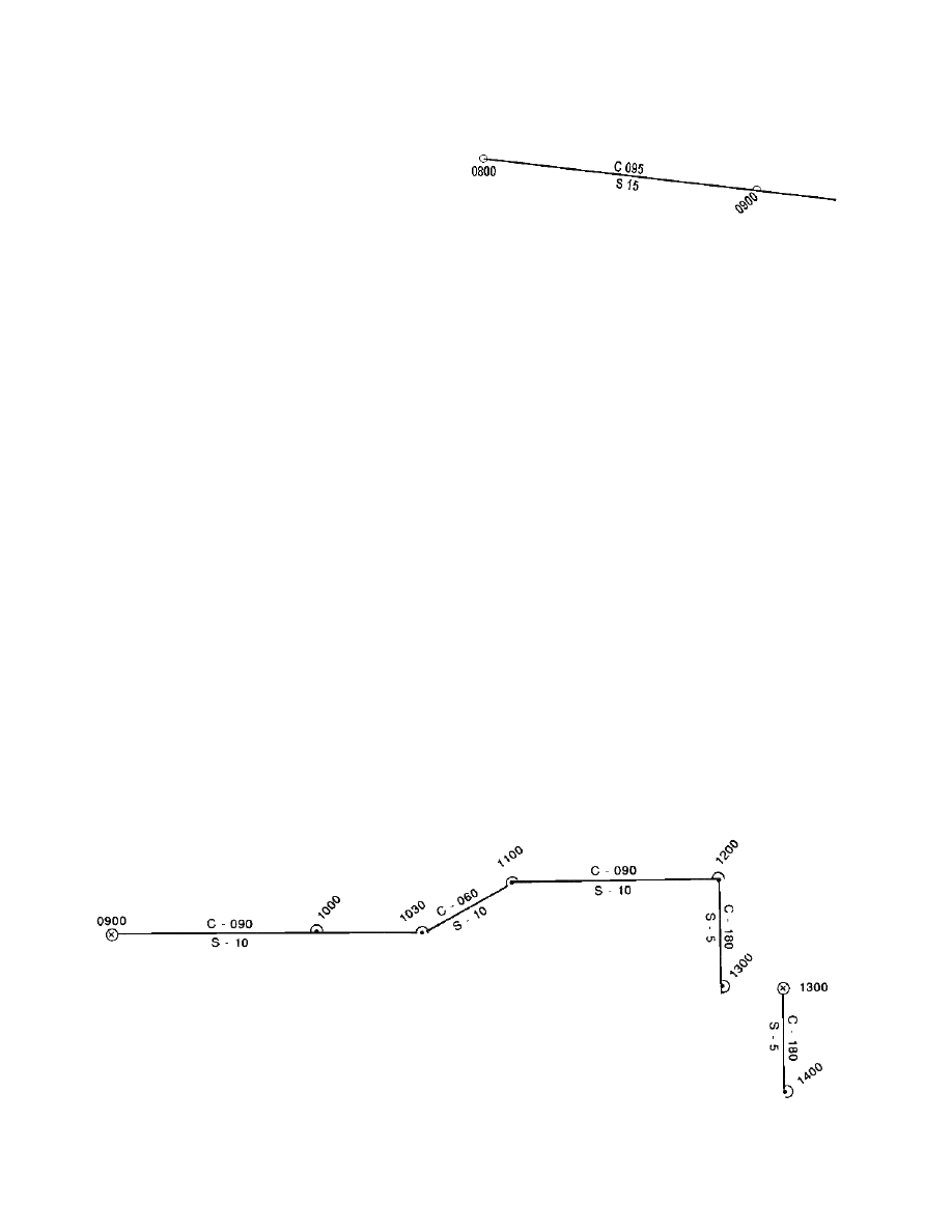
Figure 703 illustrates applying these rules. Clearing the

harbor at 0900, the navigator obtains a last visual fix. This
is called taking departure, and the position determined is
called the departure. At the 0900 departure, the conning
officer orders a course of 090

°

T and a speed of 10 knots.

The navigator lays out the 090

°

T course line from the

departure.

At 1000, the navigator plots a DR position according to

the rule requiring plotting a DR position at least every hour
on the hour. At 1030, the conning officer orders a course
change to 060

°

T. The navigator plots the 1030 DR position

in accordance with the rule requiring plotting a DR position
at every course and speed change. Note that the course line
changes at 1030 to 060

°

T to conform to the new course. At

1100, the conning officer changes course back to 090

°

T.

The navigator plots an 1100 DR due to the course change.
Note that, regardless of the course change, an 1100 DR
would have been required because of the “every hour on the
hour” rule.

Figure 702. A course line with labels.

Figure 703. A typical dead reckoning plot.

DEAD RECKONING

101

At 1200, the conning officer changes course to 180

°

T

and speed to 5 knots. The navigator plots the 1200 DR. At
1300, the navigator obtains a fix. Note that the fix position
is offset to the east from the DR position. The navigator de-
termines set and drift from this offset and applies this set
and drift to any DR position from 1300 until the next fix to
determine an estimated position. He also resets the DR to
the fix; that is, he draws the 180

°

T course line from the

1300 fix, not the 1300 DR.

704. Resetting the DR

Reset the DR plot to each fix or running fix in turn. In

addition, consider resetting the DR to an inertial estimated
position, if an inertial system is installed.

If a navigator has not taken a fix for an extended period

of time, the DR plot, not having been reset to a fix, will
accumulate time-dependent errors. Over time that error
may become so significant that the DR will no longer show
the ship’s position with acceptable accuracy. If the vessel is
equipped with an inertial navigator, the navigator should
consider resetting the DR to the inertial estimated position.
Some factors to consider when making this determination
are:

(1) Time since the last fix and availability of fix

information. If it has been a short time since the last fix and
fix information may soon become available, it may be
advisable to wait for the next fix to reset the DR.

(2) Dynamics of the navigation situation. If, for

example, a submerged submarine is operating in the Gulf
Stream, fix information is available but operational consid-
erations may preclude the submarine from going to
periscope depth to obtain a fix. Similarly, a surface ship
with an inertial navigator may be in a dynamic current and
suffer a temporary loss of electronic fix equipment. In
either case, the fix information will be available shortly but
the dynamics of the situation call for a more accurate
assessment of the vessel’s position. Plotting an inertial EP
and resetting the DR to that EP may provide the navigator
with a more accurate assessment of the navigation situation.

(3) Reliability and accuracy of the fix source. If a

submarine is operating under the ice, for example, only the
inertial EP fixes may be available for weeks at a time.
Given a high prior correlation between the inertial EP and
highly accurate fix systems such as GPS, and the continued
proper operation of the inertial navigator, the navigator may
decide to reset the DR to the inertial EP.

DEAD RECKONING AND SHIP SAFETY

Properly maintaining a DR plot is important for ship

safety. The DR allows the navigator to examine a future
position in relation to a planned track. It allows him to
anticipate charted hazards and plan appropriate action to
avoid them. Recall that the DR position is only
approximate. Using a concept called fix expansion
compensates for the DR’s inaccuracy and allows the
navigator to use the DR more effectively to anticipate and
avoid danger.

705. Fix Expansion

Often a ship steams in the open ocean for extended

periods without a fix. This can result from any number of
factors ranging from the inability to obtain celestial fixes to
malfunctioning electronic navigation systems. Infrequent
fixes are particularly common on submarines. Whatever the
reason, in some instances a navigator may find himself in
the position of having to steam many hours on DR alone.

The navigator must take precautions to ensure that all

hazards to navigation along his path are accounted for by
the approximate nature of a DR position. One method
which can be used is fix expansion.

Fix expansion takes into account possible errors in the

DR calculation caused by factors which tend to affect the
vessel’s actual course and speed over the ground. The
navigator considers all such factors and develops an
expanding “error circle” around the DR plot. One of the
basic assumptions of fix expansion is that the various

individual effects of current, leeway, and steering error
combine to cause a cumulative error which increases over
time, hence, the concept of expansion. While the errors may
in fact cancel each other out, the worst case is that they will
all be additive, and this is what the navigator must
anticipate.

Errors considered in the calculation of fix expansion

encompass all errors that can lead to DR inaccuracy. Some
of the most important factors are current and wind, compass
or gyro error, and steering error. Any method which
attempts to determine an error circle must take these factors
into account. The navigator can use the magnitude of set
and drift calculated from his DR plot. See Article 707. He
can obtain the current’s estimated magnitude from pilot
charts or weather reports. He can determine wind speed
from weather instruments. He can determine compass error
by comparison with an accurate standard or by obtaining an
azimuth of the Sun. The navigator determines the effect
each of these errors has on his course and speed over
ground, and applies that error to the fix expansion
calculation.

As noted previously, error is a function of time; it

grows as the ship proceeds along the track without
obtaining a fix. Therefore, the navigator must incorporate
his calculated errors into an error circle whose radius
grows with time. For example, assume the navigator
calculates that all the various sources of error can create a
cumulative position error of no more than 2 nm. Then his
fix expansion error circle would grow at that rate; it would

102

DEAD RECKONING

be 2 nm after the first hour, 4 nm after the second, and so on.

At what value should the navigator start this error

circle? Recall that a DR is laid out from every fix. All fix
sources have a finite absolute accuracy, and the initial error
circle should reflect that accuracy. Assume, for example,
that a satellite navigation system has an accuracy of 0.5 nm.
Then the initial error circle around that fix should be set at
0.5 nm.

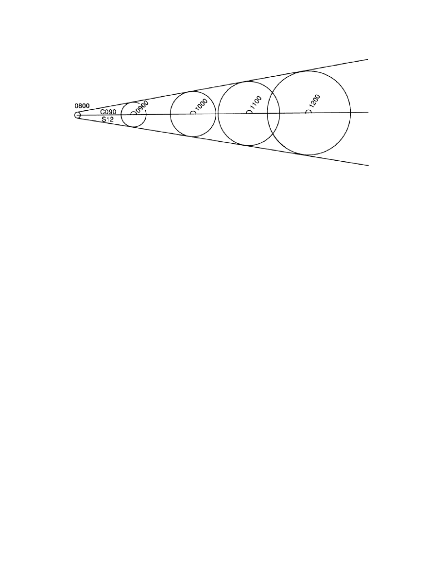
First, enclose the fix position in a circle, the radius of

which is equal to the accuracy of the system used to obtain
the fix. Next, lay out the ordered course and speed from the
fix position. Then apply the fix expansion circle to the hourly
DR’s, increasing the radius of the circle by the error factor
each time. In the example given above, the DR after one hour
would be enclosed by a circle of radius 2.5 nm, after two
hours 4.5 nm, and so on. Having encircled the four hour DR
positions with the error circles, the navigator then draws two
lines originating tangent to the original error circle and

simultaneously tangent to the other error circles. The

navigator then closely examines the area between the two

tangent lines for hazards to navigation. This technique is

illustrated in Figure 705.

The fix expansion encompasses the total area in which the

vessel could be located (as long as all sources of error are

considered). If any hazards are indicated within the cone, the

navigator should be especially alert for those dangers. If, for

example, the fix expansion indicates that the vessel may be

standing into shoal water, continuously monitor the fathometer.

Similarly, if the fix expansion indicates that the vessel might be

approaching a charted obstruction, post extra lookouts.

The fix expansion may grow at such a rate that it

becomes unwieldy. Obviously, if the fix expansion grows

to cover too large an area, it has lost its usefulness as a tool

for the navigator, and he should obtain a new fix by any

available means.

DETERMINING AN ESTIMATED POSITION

An estimated position (EP) is a DR position corrected

for the effects of leeway, steering error, and current. This
section will briefly discuss the factors that cause the DR
position to diverge from the vessel’s actual position. It will
then discuss calculating set and drift and applying these
values to the DR to obtain an estimated position. It will also
discuss determining the estimated course and speed made
good.

706. Factors Affecting DR Position Accuracy

Tidal current is the periodic horizontal movement of

the water’s surface caused by the tide-affecting gravita-
tional forces of the Moon and Sun. Current is the

horizontal movement of the sea surface caused by meteoro-
logical, oceanographic, or topographical effects. From
whatever its source, the horizontal motion of the sea’s

surface is an important dynamic force acting on a vessel.

Set refers to the current’s direction, and drift refers to

the current’s speed. Leeway is the leeward motion of a
vessel due to that component of the wind vector perpen-
dicular to the vessel’s track. Leeway and current combine
to produce the most pronounced natural dynamic effects on
a transiting vessel. Leeway especially affects sailing
vessels and high-sided vessels.

In addition to these natural forces, relatively small

helmsman and steering compass error may combine to
cause additional error in the DR.

Figure 705. Fix expansion. All possible positions of the ship lie between the lines tangent to the expanding circles.

Examine this area for dangers.

DEAD RECKONING

103

707. Calculating Set and Drift and Plotting an
Estimated Position

It is difficult to quantify the errors discussed above

individually. However, the navigator can easily quantify
their cumulative effect by comparing simultaneous fix
and DR positions. If there are no dynamic forces acting
on the vessel and no steering error, the DR position and
the fix position will coincide. However, they seldom do
so. The fix is offset from the DR by the vector sum of all
the errors.

Note again that this methodology provides no means

to determine the magnitude of the individual errors. It
simply provides the navigator with a measurable represen-
tation of their combined effect.

When the navigator measures this combined effect, he of-

ten refers to it as the “set and drift.” Recall from above that these
terms technically were restricted to describing current effects.
However, even though the fix-to-DR offset is caused by effects
in addition to the current, this text will follow the convention of
referring to the offset as the set and drift.

The set is the direction from the DR to the fix. The drift

is the distance in miles between the DR and the fix divided
by the number of hours since the DR was last reset. This is
true regardless of the number of changes of course or speed
since the last fix. The prudent navigator calculates set and
drift at every fix.

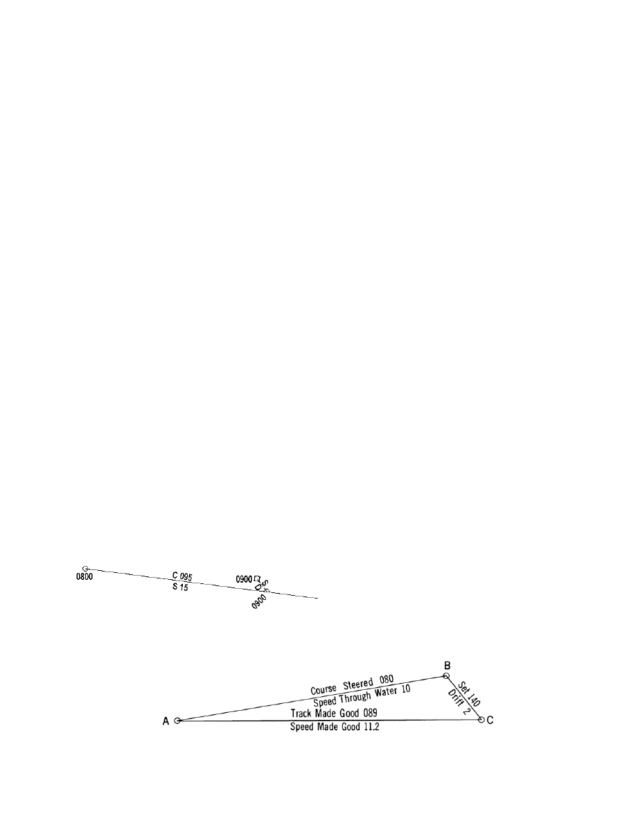
To calculate an EP, draw a vector from the DR position

in the direction of the set, with the length equal to the prod-
uct of the drift and the number of hours since the last reset.
See Figure 707. From the 0900 DR position the navigator
draws a set and drift vector. The end of that vector marks
the 0900 EP. Note that the EP is enclosed in a square and
labeled horizontally with the time. Plot and evaluate an EP
with every DR position.

708. Estimated Course and Speed Made Good

The direction of a straight line from the last fix to the

EP is the estimated track made good. The length of this
line divided by the time between the fix and the EP is the
estimated speed made good.

Solve for the estimated track and speed by using a

vector diagram. See the example problems below and refer
to Figure 708a.

Example 1: A ship on course 080

°

, speed 10 knots, is

steaming through a current having an estimated set of 140

°

and drift of 2 knots.

Required: Estimated track and speed made good.
Solution: See Figure 708a. From A, any convenient

point, draw AB, the course and speed of the ship, in
direction 080

°

, for a distance of 10 miles.

From B draw BC, the set and drift of the current, in di-

rection 140

°

, for a distance of 2 miles.

The direction and length of AC are the estimated track

and speed made good.

Answers: Estimated track made good 089

°

, estimated

speed made good 11.2 knots.

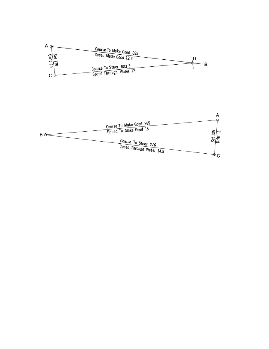
To find the course to steer at a given speed to make

good a desired course, plot the current vector from the
origin, A, instead of from B. See Figure 708b.

Example 2: The captain desires to make good a course

of 095

°

through a current having a set of 170

°

and a drift of

2.5 knots, using a speed of 12 knots.

Required: The course to steer and the speed made good.
Solution: See Figure 708b. From A, any convenient

point, draw line AB extending in the direction of the course
to be made good, 095

°

.

From A draw AC, the set and drift of the current.

Using C as a center, swing an arc of radius CD, the

speed through the water (12 knots), intersecting line AB at
D.

Measure the direction of line CD, 083.5

°

. This is the

course to steer.

Measure the length AD, 12.4 knots. This is the speed

made good.

Answers: Course to steer 083.5

°

, speed made good

12.4 knots.

Figure 707. Determining an estimated position.

Figure 708a. Finding track and speed made good through a current.

104

DEAD RECKONING

To find the course to steer and the speed to use to make

good a desired course and speed, proceed as follows:
See Figure 708c.

Example 3: The captain desires to make good a course

of 265

°

and a speed of 15 knots through a current having a

set of 185

°

and a drift of 3 knots.

Required: The course to steer and the speed to use.
Solution: See Figure 708c. From A, any convenient

point, draw AB in the direction of the course to be made

good, 265

°

and for length equal to the speed to be made

good, 15 knots.

From A draw AC, the set and drift of the current.

Draw a straight line from C to B. The direction of this

line, 276

°

, is the required course to steer; and the length,

14.8 knots, is the required speed.

Answers: Course to steer 276

°

, speed to use 14.8 kn.

Figure 708b. Finding the course to steer at a given speed to make good a given course through a current.

Figure 708c. Finding course to steer and speed to use to make good a given course and speed through the current.