Lecture Notes: Introduction to Finite Element Method Chapter 7. Structural Vibration and Dynamics

© 1999 Yijun Liu, University of Cincinnati

163

II. Free Vibration

Study of the dynamic characteristics of a structure:

•

natural frequencies

•

normal modes (shapes)

Let f(t) = 0 and C = 0 (ignore damping) in the dynamic
equation (8) and obtain

0

Ku

u

M

=

+

&

&

(12)

Assume that displacements vary harmonically with time, that
is,

),

sin(

)

(

),

cos(

)

(

),

sin(

)

(

2

t

t

t

t

t

t

ω

ω

ω

ω

ω

u

u

u

u

u

u

−

=

=

=

&

&

&

where

u

is the vector of nodal displacement amplitudes.

Eq. (12) yields,

[

]

0

u

M

K

=

−

2

ω

(13)

This is a generalized eigenvalue problem (EVP).

Solutions?

Lecture Notes: Introduction to Finite Element Method Chapter 7. Structural Vibration and Dynamics

© 1999 Yijun Liu, University of Cincinnati

164

Trivial solution:

0

u

=

for any values of

ω

(not interesting).

Nontrivial solutions:

0

u

≠

only if

0

2

=

−

M

K

ω

(14)

This is an n-th order polynomial of

ω

2

, from which we can

find n solutions (roots) or eigenvalues

ω

i

.

• ω

i

(i = 1, 2, …, n) are the natural frequencies (or

characteristic frequencies) of the structure.

• ω

1

(the smallest one) is called the fundamental frequency.

•

For each

ω

i

, Eq. (13) gives one solution (or eigen) vector

[

]

0

u

M

K

=

−

i

i

2

ω

.

i

u

(i=1,2,…,n) are the normal modes (or natural

modes, mode shapes, etc.).

Properties of Normal Modes

0

=

j

T

i

u

K

u

,

0

=

j

T

i

u

M

u

, for i

≠ j, (15)

if

j

i

ω

ω

≠

. That is, modes are orthogonal (or independent) to

each other with respect to K and M matrices.

Lecture Notes: Introduction to Finite Element Method Chapter 7. Structural Vibration and Dynamics

© 1999 Yijun Liu, University of Cincinnati

165

Normalize the modes:

.

,

1

2

i

i

T

i

i

T

i

ω

=

=

u

K

u

u

M

u

(16)

Note:

•

Magnitudes of displacements (modes) or stresses in normal
mode analysis have no physical meaning.

•

For normal mode analysis, no support of the structure is
necessary.

ω

i

= 0

⇔

there are rigid body motions of the whole or a

part of the structure.

⇒

apply this to check the FEA model (check for

mechanism or free elements in the models).

•

Lower modes are more accurate than higher modes in the
FE calculations (less spatial variations in the lower modes

⇒

fewer elements/wave length are needed).

Lecture Notes: Introduction to Finite Element Method Chapter 7. Structural Vibration and Dynamics

© 1999 Yijun Liu, University of Cincinnati

166

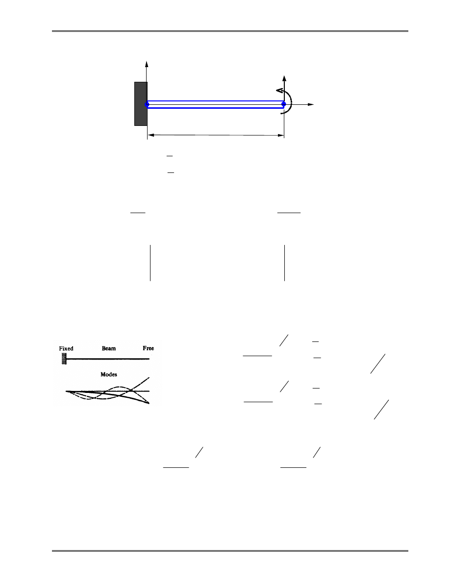
Example:

[

]

.

4

22

22

156

420

,

4

6

6

12

,

0

0

2

2

3

2

2

2













−

−

=













−

−

=













=













−

L

L

L

AL

L

L

L

L

EI

v

ρ

θ

ω

M

K

M

K

EVP:

in which

EI

AL

420

/

4

2

ρ

ω

λ

=

.

Solving the EVP, we obtain,

Exact solutions:

.

03

.

22

,

516

.

3

2

1

4

2

2

1

4

1









=









=

AL

EI

AL

EI

ρ

ω

ρ

ω

We can see that mode 1 is calculated much more accurately
than mode 2, with one beam element.

L

x

1

2

v

2

ρ, A, EI

y

θ

2

,

0

4

4

22

6

22

6

156

12

2

2

=

−

+

−

+

−

−

λ

λ

λ

λ

L

L

L

L

L

L

.

62

.

7

1

v

,

81

.

34

,

38

.

1

1

v

,

533

.

3

2

2

2

2

1

4

2

1

2

2

2

1

4

1

















=

























=

















=





















=

L

AL

EI

L

AL

EI

θ

ρ

ω

θ

ρ

ω

#1

#2

#3