1

Email Virus Propagation

Modeling and Analysis

Cliff C. Zou

∗

, Don Towsley

†

, Weibo Gong

∗

∗

Department of Electrical & Computer Engineering

†

Department of Computer Science

Univ. Massachusetts, Amherst

Technical Report: TR-CSE-03-04

Abstract

Email viruses constitute one of the major Internet security problems. In this paper we present an

email virus model that accounts for the behaviors of email users, such as email checking frequency and
the probability of opening an email attachment. Email viruses spread over a logical network defined by
email address books. The topology of email network plays an important role in determining the behavior
of an email virus spreading. Our observations suggest that the node degrees in an email network are
heavy-tailed distributed and we model it as a power law network. We compare email virus propagation
on three topologies: power law, small world and random graph topologies. The impact of the power law
topology on the spread of email viruses is mixed: email viruses spread more quickly than on a small
world or a random graph topology but immunization defense against viruses is more effective on a power
law topology.

Methods keywords: Simulations, Graph theory, Statistics.

I. I

NTRODUCTION

Computer viruses have been studied for a long time both by the research and by the application

communities. Cohen’s work [13] formed the theoretical basis for this field. In the early 1980s, viruses
mainly spread through the exchange of floppy disks. At that time, only a small number of computer
viruses existed and virus infection was usually restricted to a local area. As computer networks and the
Internet became more popular from the late 1980s on, viruses quickly evolved to be able to spread through
the Internet by various means such as file downloading, email, exploiting security holes in software, etc.

Currently, email viruses constitute one of the major Internet security problems. For example, the

Melissa virus in 1999, “Love Letter” in 2000 and “W32/Sircam” in 2001 widely spread throughout the
Internet and caused millions or even billions of dollars in damage [19][20][22]. There is, however, no
formal definition of “email virus” in the virus research area — any computer program can be called an
email virus as long as it can replicate and propagate by sending copies of itself through email messages.
While Melissa is an email virus that only uses email to propagate [21], most email viruses can also use
other mechanisms to propagate in order to increase their spreading speed on the Internet. For example,
“W32/Sircam” can spread through unprotected network shares — the shared resources that others can
access through network [23]; “Love Letter” can propagate through Internet Relay Chat (IRC) or network
shares [25]; Nimda can use four other mechanisms besides email to propagate [27].

2

Though virus spreading through email is an old technique, it is still effective and is widely used by

current viruses and worms. Sending viruses through email has some advantages that are attractive to
virus writers:

•

Sending viruses through email does not require any security holes in computer operating systems
or software.

•

Almost everyone who uses computers uses email service.

•

A large number of users have little knowledge of email viruses and trust most email they receive,
especially email from their friends [28][29].

•

Email are private properties like post office letters. Thus correspondent laws or policies are required
to permit checking email content for detecting viruses before end users receive email [18].

In order to understand how viruses propagate through email, in this paper we focus exclusively on

those email viruses that propagate solely through email, such as Melissa virus [21] (if we overlook its
slow spreading via file exchange). Thus “email virus” used in this paper is defined as a virus that only
spreads through email by including a copy of itself in the email attachment — an email user will be
infected only if he/she opens the virus email attachment. If the email user opens the attachment, the virus
program will infect the user’s computer and send itself as an attachment to all email addresses in the
user’s email address book.

A. Prior and related work

Considerable research has focused on detection and defense against email viruses. Anti-virus software

companies continuously add new techniques into their products and provide email virus defense software
such as SMTP gateway anti-virus system [17]. But little research has been pursued on modeling viruses
and worms propagation, not even to mention email viruses propagation.

Kephart, White and Chess of IBM published a series of papers from 1991 to 1993 on viral infection

based on epidemiology models [6][7][8]. [6][7] were based on a birth-death model in which viruses
were spread via activities mostly confined to local interactions. They further improved their model by
adding the “Kill signal” process and also considered the special model of viral spread in organizations
[8]. Though at that time the assumption of local interaction was accurate because of sharing disks, today
it’s no longer valid when most viruses and worms propagate through the Internet. In 2000 Wang et
al. studied a simple virus propagation model based on a clustered topology and a tree-like hierarchic
topology [9]. In their model, copies of the virus would activate at a constant rate without accounting
for any user interactions. The lack of a user model coupled with the clustered and tree-like topologies
make it unsuitable for modeling the propagation of email viruses over the Internet. Recently, Staniford et
al. studied Code Red worm propagation and presented several new techniques to improve the spreading
speed of worms [10]. The worm model considered in their paper assumes that a worm can directly reach
and infect any other computers, which is suitable for worms but not the case for email viruses — email
viruses must pass through an email network hop-by-hop.

Some researchers have studied immunization defense against virus propagation. Immunization means

that some nodes in a network are immunized and can not be infected by the virus or worm. Wang et al.
showed that selective immunization can significantly slow down virus propagation for tree-like hierarchic
topology [9]. From an email virus point of view, the connectivity of a partly immunized email network is
a percolation problem. Newman et al. derived the analytical solution of the percolation threshold of small
world topology [15][16]: if nodes are removed randomly from a small world network and the fraction of
these nodes is higher than the percolation threshold, the network will be broken into pieces. Albert et al.
were the first to explain the vulnerability of power law networks under attacks: by selectively attacking

3

the most connected nodes, a power law network tends to be broken into many isolated fragments [4].
The authors concluded that the power law topology was vulnerable under deliberate attack.

B. Our contributions

We present an email virus model that accounts for the behaviors of email users, such as email checking

frequency and the probability of opening an email attachment.

Our observation shows that the size of email groups follows a heavy-tailed distribution. Since email

network contains email groups, we believe an email network is also heavy-tailed distributed and we
model it as a power law network.

We carry out extensive simulation studies of email virus propagation. From these experiments we

derive a better understanding of the dynamics of an email virus propagation, how the degree of initially
infected nodes affects virus propagation, how the network parameters such as the power law exponent
affect virus behavior, etc.

For simplified email virus models, we mathematically prove that an email virus propagates faster as the

email checking time becomes more variable although the average email checking time does not change.

We know better of the differences among power law, small world and random graph topologies by

simulate email virus propagation on them.

We derive by simulations the selective percolation curves and thresholds for the power law, small world

and random graph topologies. These selective percolation curves can explain why selective immunization
defense against virus spreading is quite effective for a power law topology but not so good for the other
two topologies.

C. Organization of the paper

The rest of the paper is organized as follows: We present the email virus model in Section II. In

Section III we discuss the email network topology and model it as a power law topology. In Section
IV, we present simulation studies of email virus propagation without considering immunization. We also
compare virus spreading among power law, small world and random graph topologies. In Section V, we
study the immunization defense against email viruses and the corresponding percolation problem. Section
VI concludes this paper with some discussions.

II. E

MAIL VIRUS PROPAGATION MODEL

Because of the complexity of an email network and the randomness of email users’ behaviors, it’s

difficult to mathematically analyze email virus propagation. Thus in this paper we will rely primarily on
simulation rather than mathematical analysis. In this way we can focus on realistic scenarios of email
virus propagation.

In this paper, we consider email viruses that only transfer through users’ email address books. Thus

email address relationship between users’ address books forms a logical network for email viruses. Strictly
speaking, the email logical network is a directed graph: each vertex in the graph represents an email
user while a directed edge from node A to node B means that user B’s email address is in user A’s
address book. Email address book of a user usually contains the user’s friends’ or business partners’
email addresses. Thus if user A has user B’s address, user B probably also has user A’s address in his
own address book, which means that many of the directed edges on the email network point to both
direction. Although this may not always be true, we model the email network as an undirected graph in
this paper.

4

We represent the topology of the logical email network by an undirected graph

G =< V, E >, ∀v ∈ V ,

v denotes an email user and ∀e = (u, v) ∈ E, u, v ∈ V , represents two users u and v that have the email
address of each other in their own address books.

|V | is the total number of email users.

Let’s first describe the email virus propagation scenario captured by our model: users check their email

from time to time. When a user checks his email and encounters a message with a virus attachment, he
may discard a message with a viral attachment (if he suspects the email or detects the email virus by
using anti-virus software) or open the virus attachment if unaware of it. When the virus attachment is
opened, the virus immediately infects the user and sends out virus email to all email addresses on this
user’s email address book. The infected user will not send out virus email again unless the user receives
another copy of the virus email and opens the attachment again.

From the above description, we see that email viruses, not like worms, depend on email users’

interaction to propagate. There are primarily two human behaviors affecting email viruses: one is the
email checking time, denoted by

T

i

,

i = 1, 2, · · · , |V |, the time interval when user i checks email; another

is the opening probability, denoted by

P

i

,

i = 1, 2, · · · , |V |, the probability with which user i opens a

virus attachment.

The email checking time

T

i

of user

i, i = 1, 2, · · · , |V |, is a random variable with an average email

checking time,

E[T

i

], determined by user i’s habits. We assume that when a user checks his email, he

checks all new email in his mailbox. The opening probability

P

i

of user

i is determined by the user’s

awareness and knowledge of email viruses.

We assume that each user’s behaviors are independent of each other. We model

T

i

and

P

i

,

i =

1, 2, · · · , |V |, as follows:

•

Email checking time

T

i

of user

i, i = 1, 2, · · · , |V |, is exponentially distributed with the mean E[T

i

].

We assume that

E[T

i

] is itself a random variable, which we denote as T .

•

User

i opens a virus attachment with probability P

i

when he checks any virus email. Let

P denote

the random variable that generates

P

i

,

i = 1, 2, · · · , |V |.

•

Since the number of email users,

|V |, is very large and a user’s behaviors are independent of

others, we assume that

T and P are independent Gaussian random variables, i.e., T ∼ N (µ

T

, σ

2

T

),

P ∼ N (µ

P

, σ

2

P

), i = 1, 2, · · · , N.

An email user is called infected once the user opens a virus email attachment. Let

N

0

denote the

number of initially infected users that send out virus email to all their neighbors at the beginning of a
virus propagation. Let random variable

N

t

denote the number of infected users at time

t during email

virus propagation,

N

0

≤ N

t

≤ |V |, ∀t > 0.

It takes time before a recipient receives a virus email sent out by an infected user. But the email

transmission time is usually much smaller comparing to a user’s email checking time (the time interval
between a user’s two consecutive email checking). Thus in our model we ignore the email transmission
time.

Table. I lists most of the notations used in this paper.

III. E

MAIL NETWORK TOPOLOGY DISCUSSION

The email network is determined by users’ email address books. The size of a user’s email address

book is the degree of the corresponding node in the network graph. Since email address books are private
property, we have no such data to tell us what the email topology is. We have, however, examined the
sizes of the more than 800,000 email groups in Yahoo! [11]. Thus we can use it to figure out what
the topology might be like although the topology of email groups is not the complete email network
topology.

5

TABLE I

N

OTATIONS USED IN THIS PAPER

Notation

Explanation

G =< V, E >

Undirected graph representing the email network.

v ∈ V denotes an email user, |V | is user population.

T

i

Email checking time of user

i — the time interval between user i’s two consecutive email

checking,

i = 1, 2, · · · , |V |. T

i

is exponentially distributed with mean value

E[T

i

].

E[T

i

]

Average email checking time of user

i, i = 1, 2, · · · , |V |.

P

i

Opening probability of user

i — the probability with which user i opens a virus attachment, i = 1, 2, · · · , |V |.

T

Gaussian-distributed random variable that generates

E[T

i

], i = 1, 2, · · · , |V |. T ∼ N(µ

T

, σ

2

T

).

P

Gaussian-distributed random variable that generates

P

i

,

i = 1, 2, · · · , |V |. P ∼ N (µ

P

, σ

2

P

).

N

0

Number of initially infected users at the beginning of virus propagation.

N

t

Number of infected users at time

t, ∀t > 0.

E[N

t

]

Average number of infected users at time

t, ∀t > 0.

V

t

Number of virus email in the system at time

t, ∀t > 0.

α

Power law exponent of a power law topology that has complementary cumulative degree distribution

F (d) ∝ d

−α

.

N

h

∞

Number of users that are not infected when virus propagation is over.

D

t

Average degree of nodes that are healthy before time

t but are infected at time t, ∀t > 0.

C(p)

Connection ratio — the percentage of remaining nodes still connected
after removal of the top

p percent of most connected nodes from a network.

L(p)

Remaining link ratio — fraction of links remaining after removal of the top

p percent of most connected nodes.

As mentioned in Section II, we model the email network as an undirected graph

G =< V, E >. Let

f (d) be the fraction of nodes with degree d in G. The complementary cumulative distribution function
(ccdf) is denoted by

F (d) =

∞

i=d

f (i), i.e., the fraction of nodes with degree greater than or equal to

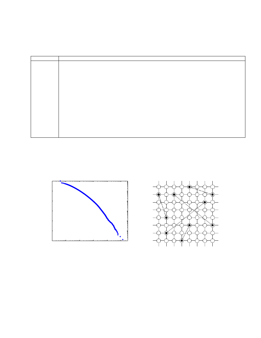
d. We present the Yahoo! empirical ccdf of the group sizes for May 2002 in the log-log format Fig. 1.

1

10

100

1,000

10,000

100,000

1e−6

1e−5

0.0001

0.001

0.01

0.1

1

Yahoo Group Size (May 2002)

Group size (d)

F(d)

Fig. 1.

Complementary cumulative distr. of Yahoo!

group size

Fig. 2.

Illustration of a two-dimensional

small world network

The size of Yahoo! groups varies from as low as 4 to more than 100,000. From Fig. 1 we can see that

the size of Yahoo groups is heavy-tailed distributed, i.e., the ccdf

F (d) decays slower than exponentially

[12].

Currently, email lists, or called email groups, have become very popular. Once a user puts the address

of an email list in his address book, from the virus point of view, the address book virtually has all the
addresses contained in the email list. Since email groups are heavy-tailed distributed as shown in Fig. 1,
it is reasonable to believe that email network is also heavy-tailed distributed.

6

In order to study email virus propagation, we need to use a network generator to create the email

networks. In this paper we use the GLP power law topology generator [1] to generate power law topologies
to represent email networks with a heavy-tailed node degree distribution. A power law topology is heavy-
tailed distributed and has the power law ccdf

F (d) ∝ d

−α

[1], which is linear on a log-log plot [3].

Except power law topology generators, there is no other network generator available to create a heavy-
tailed distributed topology. Thus a power law topology generator is the best candidate to generate the
email network although the size of Yahoo! groups and the degree of a real email network may not be
strictly power law distributed.

There are some other popular topologies such as random graph topology [14] and small world topology

[2]. They are not suitable for the email network because they do not provide heavy-tailed node degree
distributions. However, we study email virus propagation on these two topologies in order to understand
how different topologies affect email virus propagation.

In this paper, a random graph network of

n vertices and average degree k ≥ 2 is constructed as follows.

Begin with

n vertices and no edges. In order to produce a connected network, we first add n edges one

by one: edge

i, i = 1, 2, · · · , n, connects vertex i to another randomly chosen vertex. Then at each step

two randomly chosen vertices are connected with an edge until the total number of edges reaches

nk/2.

We generate the small world network by using the model in [16], which is depicted in Fig. 2: on

two-dimensional lattice each one of additional links randomly selects two nodes on the lattice to connect.

IV. E

MAIL VIRUS SIMULATION STUDIES

We are interested in

E[N

t

] — the average number of infected users at any time t. We derive E[N

t

] by

averaging the results of

N

t

from many simulation runs that have the same inputs but different random

seeds.

Discrete-time simulation has been used in many viruses and worms modeling papers [8][9][10]. Thus

we simulate our email virus model in discrete time, too. Before the start of virus propagation, we first
assign

P

i

and

E[T

i

] for each user i, i = 1, 2, · · · , |V | as follows:

P

i

=






P 0 ≤ P ≤ 1

0 P < 0

1 P > 1

(1)

E[T

i

] = max{T, 1}

(2)

where both random variables

T and P are Gaussian-distributed and are defined in Section II ( see Table.

I).

At each discrete time clock

t, t = 1, 2, 3, · · · , if user i opens an email virus attachment, the virus will

send out virus email to all user

i’s neighbors. These in turn will affect the activities of user i’s neighbors

at or after the subsequent time

t + 1. After user i checks email at time t, a new email checking time

T

i

is assigned to this user in order to determine when he will check email again. In the discrete-time

simulation model,

T

i

is a positive integer derived by:

T

i

= max{X, 1}

(3)

where random variable

X is exponentially distributed with mean value E[T

i

] derived from (2).

For most experiments in the following, we perform 100 simulation runs to derive the average value

E[N

t

]. The underlying power law network has 100,000 nodes, average degree 8 and power law exponent

α = 1.7. Other simulation parameters are: T ∼ N (40, 400), P ∼ N (0.5, 0.09) and N

0

= 2. Initially

infected nodes are randomly chosen in each simulation run. We use the same power law network and
the same parameters in all simulations if not mentioned explicitly.

7

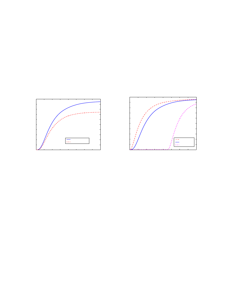
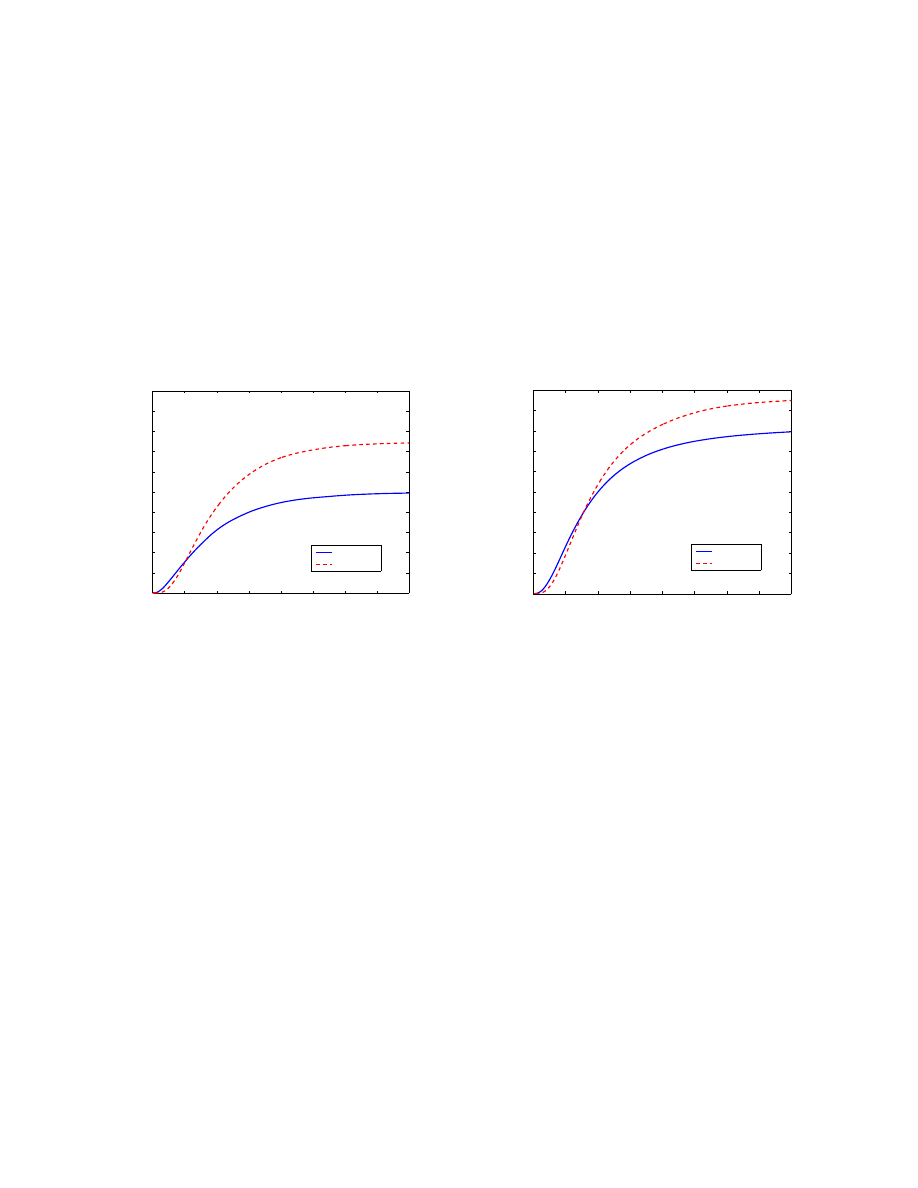
A. Reinfection vs. Non-reinfection

First we consider two cases under different infection assumptions: the reinfection case versus the non-

reinfection case. Reinfection means that a user will send out email virus copies whenever he opens a
virus email attachment. Thus a recipient can repeatedly receive virus email from the same infected user.
Non-reinfection means that each infected user sends out virus copies only once, after which he will not
send out any virus email even if he opens virus attachment again. Some email viruses belong to the
non-reinfection case, such as Melissa and “Love Letter” [21][26]. Others belong to reinfection case, such
as “W32/Sircam” [23][24].

Fig. 3 illustrates the behavior of

E[N

t

] as a function of time t for both the reinfection case and

non-reinfection case.

0

50

100

150

200

250

300

350

400

0

1

2

3

4

5

6

7

8

9

10

x 10

4

Reinfection vs. Non−reinfection

Time: t

E[N

t

]

Reinfection
Non−reinfection

Fig. 3.

Reinfection vs. non-reinfection

0

50

100

150

200

250

300

350

400

0

1

2

3

4

5

6

7

8

9

10

x 10

4

Random effect in simulation (reinfection case)

Time: t

N

t

Maximum
Mean value
Minimum

Fig. 4.

Random effect in simulation (reinfection case)

In our email virus model, each user

i opens an email attachment with probability P

i

when he checks

any virus email. Thus if user

i receives m virus email, he has the probability 1 − (1 − P

i

)

m

to be infected

— his chance of being infected increases as a function of the amount of virus email that he receives.
For this reason more users are infected in the reinfection case than in the non-reinfection case as shown
in Fig. 3.

Since some users open email attachment with very low probability, in both cases a certain number of

users will not be infected when the virus propagation is over. Let

N

h

∞

denote the number of users that

are not infected when virus propagation is over. We can derive some analytical results for

N

h

∞

for the

non-reinfection case because the virus propagation of this case is relatively simple.

In the non-reinfection case, each infected user sends out only once the virus copies to all of his

neighbors. Thus user

i who has m

i

links will receive at most

m

i

copies of virus email — the probability

that user

i is not infected is at least (1−P

i

)

m

i

. For the non-reinfection case, we can derive a lower bound

for

E[N

h

∞

] if we know the network degree distribution and assume that P

i

is the same for all users.

Let

G(x) denote the probability generating function of the degree of the email network:

G(x) =

∞

k=1

P (d = k)x

k

(4)

where

P (d = k) is the probability a node has degree k. In the case that all users are equally likely to

8

open virus attachments, i.e.,

P

i

= p, ∀i ∈ {1, 2, · · · , |V |}, we can get a lower bound for E[N

h

∞

]:

E[N

h

∞

] ≥ |V |

∞

k=1

P (d = k)(1 − p)

k

= |V |G(1 − p)

(5)

where

|V | is the user population.

Fig. 4 shows how variable each simulation run can be. For each time

t we get the maximum, average

and minimum values among the previous 100 simulation runs and plot the three maximum, average and
minimum simulation curves, respectively ( reinfection case). We observe that the initial phase of virus
spreading determines the overall propagation speed.

The email virus has successfully spread out in all 100 simulation runs in Fig. 4. In fact, the email virus

has a small chance to die before it spreads out. For example, in the beginning those initially infected
users send out virus copies to their neighbors. If all their neighbors decide not to open email attachment
for the first round, then no virus email exists in the network after those neighbors finish checking email
for the first time. If we assume that all users open virus attachments with the same probability

p and

the number of virus copies sent out by those initially infected users is

m, then the email virus has the

probability

(1 − p)

m

to die before it infects any users besides those initially infected ones.

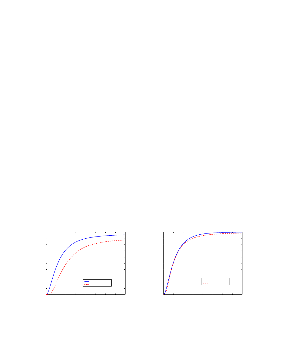
B. Initially infected users with highest degree vs. lowest degree

In our previous experiment, the degree of the power law network varies from

3 to 1833. It seems that

the degree of initially infected nodes, i.e., the size of email address books of initially infected users, is
important to email virus propagation. We consider two cases: in the first case the initially infected nodes
have the highest degree while in the second case the initially infected nodes have the lowest degree.
Both cases have the same number of initially infected nodes, i.e.,

N

0

= 2. Fig. 5 shows the behavior of

E[N

t

] as a function of time t of these two cases on two power law networks, respectively. Both power

law networks have the same

100, 000 nodes and power law exponent α = 1.7 but different connection

density — one has average degree

8 while the other one has average degree 20.

All simulations here belong to the reinfection scenario. In the following all email virus propagation

simulations belong to the reinfection scenario if not mentioned explicitly.

0

50

100

150

200

250

300

350

400

0

1

2

3

4

5

6

7

8

9

10

x 10

4

Effect of different initially infected nodes

Time: t

E[N

t

]

Highest degree
Lowest degree

a. Network with average degree

8

0

50

100

150

200

250

300

350

400

0

1

2

3

4

5

6

7

8

9

10

x 10

4

Effect of different initially infected nodes

Time: t

E[N

t

]

Highest degree
Lowest degree

b. Network with average degree

20

Fig. 5.

Effect of different degrees of initially infected nodes

Fig. 5 shows that the identities of the initially infected nodes are more important in a sparsely connected

network than a densely connected network. From a virus writer’s point of view, it’s important to let his

9

virus spread as widely as possible before people become aware of the virus or have anti-virus patches
available. It will help the virus to propagate by choosing the right initial launching points such that those
initially infected users have large email address books.

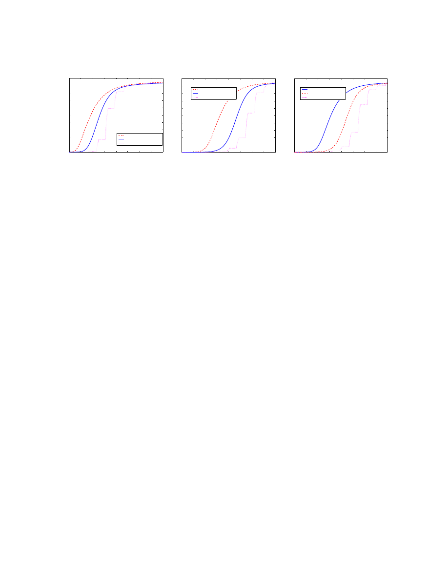
C. Topology effect: Power law, Small world and Random graph

In Section III, we discussed why we believe the email logical network is a heavy-tailed network. In

this section we examine how topology affects email virus propagation.

We run our email virus simulation on a power law network, a small world network and a random

graph network, respectively. All three networks have the same average degree

8 and 100, 000 nodes.

Fig. 6 shows the

E[N

t

] as a function of time t of these three topologies for non-reinfection case and

reinfection case, respectively.

0

50

100

150

200

250

300

350

400

0

1

2

3

4

5

6

7

8

9

10

x 10

4

Email virus propagation on different topologies

Time: t

E[N

t

]

Power law topology
Random graph topology
Small world topology

a. Non-reinfection case

0

50

100

150

200

250

300

350

400

0

1

2

3

4

5

6

7

8

9

10

x 10

4

Email virus propagation on different topologies

Time: t

E[N

t

]

Power law topology
Random graph topology
Small world topology

b. Reinfection case

Fig. 6.

Effect of topology on email virus propagation

Fig. 6 shows that virus propagation on the small world network is very similar to the one on the

random graph network. It is not a surprising result if we think about the relationship between a small
world and a random graph topology: small world topology and random graph topology have the similar
characteristic path length while small world topology has much larger clustering coefficient than random
graph topology has[2].

Characteristic path length is defined as the number of edges in the shortest path between two vertices,

averaged over all pairs of vertices [2]. For the email network, characteristic path length corresponds to
the average number of friendships in the shortest chain connecting two users. The definition of clustering
coefficient is complex but for the email network it measures the cliquishness of a typical friendship circle
[2] — what matters to the speed of email virus propagation is the characteristic path length, not the
clustering coefficient.

From Fig. 6 we observe that the virus infection speed on power law topology is much greater than the

speed on either a small world or random graph topology. One reason is that the characteristic path length
of a power law network is smaller than the one of a small world or a random graph network [1][5], the
virus can reach and infect a node earlier by passing through a shorter path on a power law network than
on a small world or a random graph network.

Another reason is that an email virus exhibits more “firing power” on a power law network at the early

stage of virus propagation. On a power law network, the degree of different nodes varies significantly
[3]. Once the virus infects some highly connected nodes, a much larger number of virus copies will be

10

sent out from these nodes. Thus the infection speed will be “amplified” by these highly connected nodes.
Neither a small world nor a random graph network exhibits such amplification because all nodes on these
networks have a similar degree.

Let

D

t

denote the average degree of nodes that are healthy before time

t but are infected at time t.

D

t

tells us what kind of node is being infected at each time

t, t = 1, 2, 3, · · · . We repeat the experiment

in Fig. 6(b) and derive

D

t

for each topology by averaging the results of

1, 000 simulation runs. We plot

each

D

t

of these three networks as a function of time

t in Fig. 7. Note that D

t

is very similar in small

world and random graph networks.

0

20

40

60

80

100

120

140

5

10

15

20

25

30

35

40

45

50

Average degree of nodes that are being infected at each time tick

Time: t

D

t

Power law topology
Random graph topology
Small world topology

Fig. 7.

Average degree of nodes that are being infected at each time tick

Fig. 7 clearly shows that email virus propagation on power law network has two phases. In the

beginning, virus will infect the most highly connected nodes. Later on it will primarily attempt to infect
nodes that have small degree. These two phases are not exhibited by either a small world network or a
random graph network.

In the non-reinfection case, once the virus propagation is over, more nodes remain healthy on a power

law topology than on a small world or a random graph topology (see Fig. 6(a)). As explained in the first
experiment, the probability that a node will be infected decreases as the degree does. Since these three
topologies have the same average degree, compared to the small world and random graph topologies,
more nodes in the power law topology have degree less than the average degree. Thus more nodes in
the power law topology will remain healthy at the end of the virus propagation than in the other two
topologies.

We also investigate the sensitivity of our results to tenfold increase in the number of users by running

the same simulations as in Fig. 6 where the number of nodes is

1, 000, 000 and average degree remains

8. we observe the same behaviors of virus propagation on tenfold larger networks for all three topologies.
The results show that the behavior of virus propagation doesn’t change when the network scale changes.

D. Effect of the power law exponent

α

The power law exponent

α is an important parameter for a power law topology. It is the slope of the

curve of the complementary cumulative degree distribution in a log-log graph [1] — the smaller

α is, the

more variable is the degree of the topology. In our previous simulations, we use

α = 1.7 to generate the

power law network with

100, 000 nodes and average degree 8. This power law network has the highest

degree 1833 and the lowest degree 3. Since the degree corresponds to the size of email address book,
we think

α = 1.7 will give us a reasonable power law email network that has 100, 000 nodes.

11

The Internet AS level power law topology has the power law exponent

α = 1.1475 [1]. Using α =

1.1475 for a 100, 000 nodes power law network with average degree 8 will produce a network with the
highest degree up to

28, 000 and lowest degree of 1. Thus we think α = 1.1475 is too small for modeling

the email network.

However, we don’t know the value of

α for the real email network. In order to see how the power

law exponent

α affects virus propagation, we compare virus propagation on the following two power law

networks: one has

α = 1.7 and the other one has α = 1.1475. Both networks have 100, 000 nodes and

average degree

8. We denote the network with α = 1.7 as the power law network Net

a

and the network

with

α = 1.1475 as the power law network N et

b

.

E[N

t

] is plotted for both networks as functions of

time

t in Fig. 8 for the non-reinfection and reinfection cases, respectively.

0

50

100

150

200

250

300

350

400

0

1

2

3

4

5

6

7

8

9

10

x 10

4

Effect of the power law exponent

α

Time: t

E[N

t

]

α

=1.1475

α

=1.7

a. Non-reinfection case

0

50

100

150

200

250

300

350

400

0

1

2

3

4

5

6

7

8

9

10

x 10

4

Effect of the power law exponent

α

Time: t

E[N

t

]

α

=1.1475

α

=1.7

b. Reinfection case

Fig. 8.

Effect of power law exponent

α on email virus propagation

For both cases, Fig. 8 shows that an email virus initially propagates faster on power law network

N et

b

than on

N et

a

. Later, however, the virus spreads more quickly on

N et

a

than on

N et

b

.

Power law network

N et

b

concentrates a large number of links on a small number of nodes. Once

some of these have been infected, there will be more copies of virus sent out than in network

N et

a

.

Those highly connected nodes are like “virus amplifiers” in email virus propagation. Thus the initial
virus infection speed is larger on

N et

b

than on

N et

a

.

After having infected most highly connected nodes, the email virus enters the second phase, mainly

trying to infect the nodes that have small degree. In power law network

N et

b

, more nodes have smaller

degree than in network

N et

a

— the smallest degree in

N et

b

is one while in

N et

a

it is three. A node

with a smaller number of links than another node is less likely to receive virus email. Thus during the
second phase of virus propagation, the virus infection speed in

N et

b

is smaller than the speed in

N et

a

.

E. Effect of email checking time variability

In our email virus model, we assume that user

i’s email checking time, T

i

, is exponentially distributed

with mean

E[T

i

], i = 1, 2, · · · , |V |. What if the email checking time is drawn from some other dis-

tributions, like Erlang distribution, or is simply a fixed value? What effect will the variability of email
checking time have on the email virus propagation?

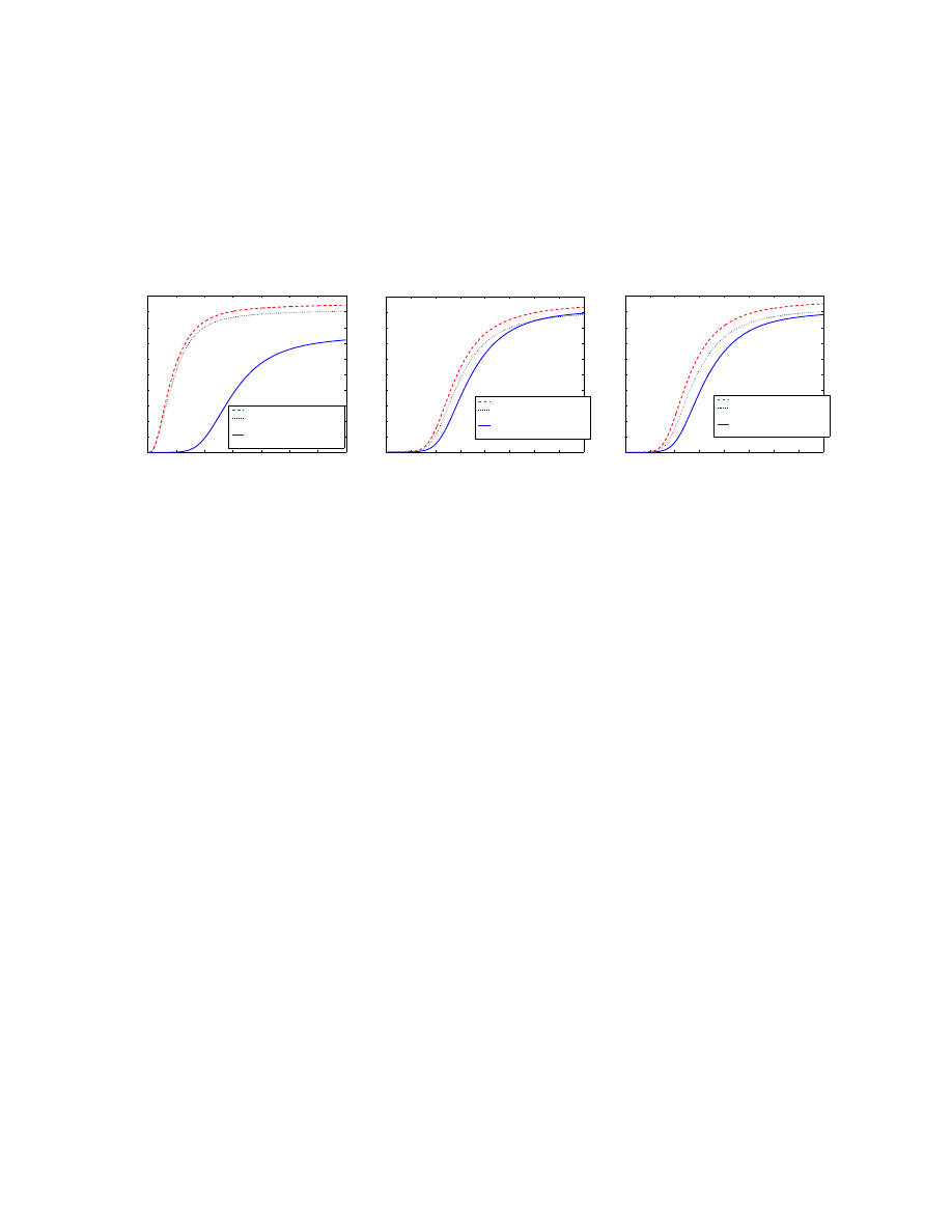
Fig. 9 shows the average number of infected users,

E[N

t

], under three different simulation cases (on

a power law network, a small world network and a random graph network, respectively). In order to
study the effect of the variability of email checking time without other disturbance, we let all users have

12

0

50

100

150

200

250

300

350

400

0

1

2

3

4

5

6

7

8

9

10

x 10

4

Effect of email checking time variability

Time: t

E[N

t

]

Exponential distribution
Erlang distribution
Constant value

a. Power law topology

0

50

100

150

200

250

300

350

400

0

1

2

3

4

5

6

7

8

9

10

x 10

4

Effect of email checking time variability

Time: t

E[N

t

]

Exponential distribution
Erlang distribution
Constant value

b. Small world topology

0

50

100

150

200

250

300

350

400

0

1

2

3

4

5

6

7

8

9

10

x 10

4

Effect of email checking time variability

Time: t

E[N

t

]

Exponential distribution
Erlang distribution
Constant value

c. Random graph topology

Fig. 9.

Effect of the variability of email checking time on virus propagation

the same average email checking time

E[T

i

] = L, ∀i ∈ {1, 2, · · · , |V |}. In the first case we let email

checking time be exponentially distributed with mean value

L. In the second case we use a 3rd-order

Erlang distribution with mean value

L. In the third case all users have a constant email checking time

L. In the simulations of Fig. 9, we let L = 40. For each simulation runs we randomly select 10 nodes
as initially infected nodes, i.e.,

N

0

= 10.

Given the same mean value

L the exponential distribution is more stochastically variable [30] than

the kth-order Erlang distribution where

k > 1. Both of them are more stochastically variable than the

constant value

L. Fig. 9 shows the same relationship among these three cases on all topologies: virus

propagation speed is not only determined by the average spreading time, but also is affected by the
variability of the spreading time — an email virus propagates faster as the email checking time becomes
more variable.

Unfortunately, email virus propagation is a very complex process that we can’t strictly prove the above

conclusion. But for certain simplified email virus models, we can derive the formula of

E[N

t

] and show

why the variability of email checking time counts. The intuitive answer is what we refer to as the so
called snowball effect: before virus copies in the system with less variable checking time give birth to the
next generation — infecting some new users, virus copies in another system with more variable checking
time have already given birth to several generations although each generation’s population is relatively
small.

We introduce the simplified model in the following: suppose the email virus propagation is a discrete-

time process as we have used in our simulations. A user always opens an email virus attachment when he
checks email. Once an email virus attachment is opened, it sends virus email to

C vulnerable users. Last,

we assume the user population is infinite. Each vulnerable user that receives virus email only receives
one copy — no virus email will be wasted trying to infect an infected user again. When an email virus
copy is activated by a user, it infects the user, generates

C new copies of virus email, and then disappears.

Suppose at the beginning,

t = 0, all users are vulnerable but not infected, i.e. N

0

= 0, and V

0

users

have one copy of virus email on each of them. Let

V

t

denote the number of virus copies existing in the

system at time

t. Note that V

t

= N

t

,

t > 0 and C is a positive integer.

Let’s compare the following two cases: In the first case every user has a constant email checking time

denoted by

L (L is a positive integer) while in the second case every user has an exponentially distributed

email checking time with mean

L. Thus all users have the same average email checking time in these

two cases.

For the first case, the virus propagation is a deterministic process.

N

t

and

V

t

are updated only when

13

t = kL, k = 1, 2, 3, · · · :






V

(k+1)L

= CV

kL

N

(k+1)L

= V

kL

+ N

kL

N

0

= 0

k = 0, 1, 2, 3, · · ·

(6)

Note that

L is the mean email checking time for all users, C is the number of virus email sent out by

an infected user. From the iterative equation (6), we get:

N

t

=

V

0

t/L

if

C = 1

V

0

(C

t/L

− 1)/(C − 1) if C > 1

t = 1, 2, 3, · · ·

(7)

For the second case where email checking time is a random variable, we can use the mean value analysis

to get the average value

E[N

t

] and E[V

t

]. Since the email checking time is exponentially distributed with

mean

L, at any time t + 1, each one of the existing V

t

virus copies has probability

(1 − e

−1/L

) of being

opened by the user who receives it regardless of what the time

t is and how long the virus copy has been

received by the user. Thus we can derive the following recursive equation describing

E[N

t

] and E[V

t

]:






E[V

t+1

]

= e

−1/L

E[V

t

] + C(1 − e

−1/L

)E[V

t

]

E[N

t+1

]

= E[N

t

] + (1 − e

−1/L

)E[V

t

]

E[N

0

] = 0

E[V

0

] = V

0

, t = 0, 1, 2, 3, · · ·

(8)

From the equation (8), we get:

E[N

t

] =

V

0

(1 − e

−1/L

)t

if

C = 1

V

0

[C(1−e

−1/L

)+e

−1/L

]

t

C−1

if

C > 1

t = 1, 2, 3, · · ·

(9)

Comparing equation (7) and (9), if

C = 1, it’s hard to tell in which case an email virus propagates

faster. But what we are interested is the normal situation where

C ≥ 2 and L ≥ 2. When L ≥ 3 and

C = 2, or L ≥ 2 and C ≥ 3, E[N

t

] in the equation (9) is always larger than N

t

in the equation (7),

∀t ≥ 1. This means that a more variable checking email time can help the virus to propagate faster.

Here we rely heavily on the memoryless property of the exponential distribution in our analysis. Hence

we have been unsuccessful in obtaining an expression for

E[N

t

] for other distributions.

V. I

MMUNIZATION

, P

ERCOLATION FOR

E

MAIL

V

IRUS

D

EFENSE

In this section, we consider immunization defense against email virus. For the email network, immu-

nizing a node means that the node can’t be infected by the virus. In this paper we consider a static
immunization defense. By this we mean that before an email virus starts to propagate, a small number
of nodes in the network have already been immunized. If some email users are well educated and they
never open suspicious email attachment, they can be treated as immunized nodes in the email network.

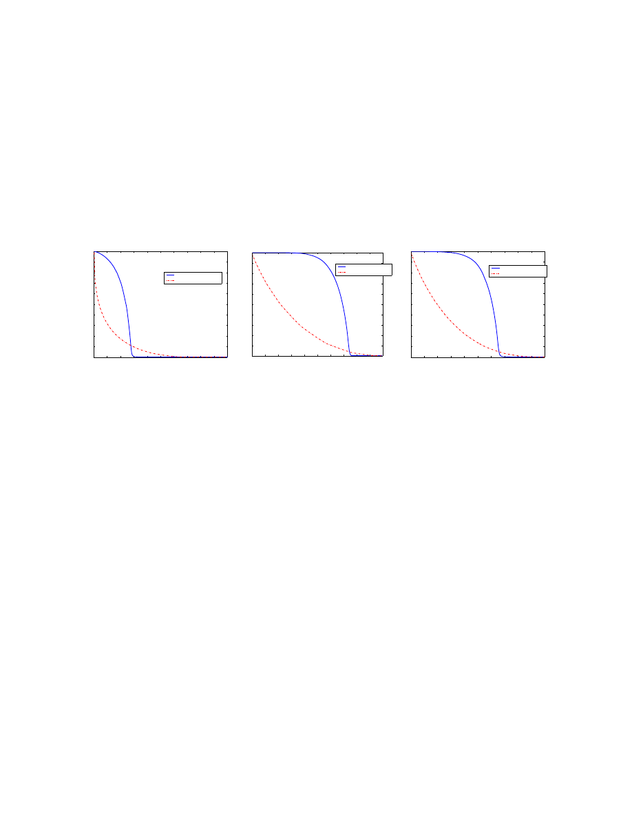
A. Effect of selective immunization

It’s unfeasible for us to immunize all email users, i.e., immunize all nodes in the email network. A

realistic approach is to immunize a subset of nodes. Thus we need to know how to choose the appropriate
size and the membership of this subset in order to slow down or constrain the email virus spreading as
best as we could.

Wang et al. explained that selective immunization could significantly slow down virus propagation for

tree-like hierarchic topology [9]. We find that for power law email network, selecting highly connected
nodes to immunize is also quite effective against virus propagation.

14

We simulate virus propagation under two different immunization defense methods: in the first case we

randomly choose 5% nodes to immunize while in the second case we choose 5% most connected nodes
to immunize. We plot

E[N

t

] as a function of time t for these two immunization methods in Fig. 10 (on

a power law network, a small world network and a random graph network, respectively). In order to see
the effect of immunization, we also plot

E[N

t

] for the original case where there is no immunization.

0

100

200

300

400

500

600

700

0

1

2

3

4

5

6

7

8

9

10

x 10

4

Effect of selective immunization

Time: t

E[N

t

]

No immunization
5% randomly selected nodes
immunization
5% most connected nodes
immunization

a. Power law topology

0

50

100

150

200

250

300

350

400

0

1

2

3

4

5

6

7

8

9

10

x 10

4

Effect of selective immunization

Time: t

E[N

t

]

No immunization
5% randomly selected nodes
immunization
5% most connected nodes
immunization

b. Small world topology

0

50

100

150

200

250

300

350

400

0

1

2

3

4

5

6

7

8

9

10

x 10

4

Effect of selective immunization

Time: t

E[N

t

]

No immunization
5% randomly selected nodes
immunization
5% most connected nodes
immunization

c. Random graph topology

Fig. 10.

Effect of selective immunization on email virus propagation (reinfection case)

We observe from Fig. 10 that selective immunization plays an important role for a power law topology

while it has little effect for a small world topology or a random graph topology. On a power law email
network, we can significantly slow down email virus propagation by selecting those most connected
nodes to immunize.

The results here are consistent with the conclusions in [4]. The authors in [4] showed that selectively

attacking the most connected nodes rapidly increases the diameter of a power law network. Since an
email virus depends on the connectivity of the email network to spread, immunizing the most connected
nodes has the effect of rapidly increasing the network diameter. This in turn significantly slows down
virus propagation.

B. Selective percolation and email virus prevention

We have observed that selective immunization is quite effective for a power law email network. Then

what is the appropriate size of the subset to immunize? How many nodes do we need to immunize in
order to prevent an outbreak of an email virus?

From an email virus point of view, the connectivity of a partly immunized email network is a percolation

problem. Newman et al. derived the analytical solutions of percolation on small world networks [15][16].
The “percolation” in these paper means removing some nodes from the networks uniformly. Since we
want to study the effect of selective immunization, we introduce the corresponding concept selective
percolation. For example, a selective percolation value is

p means to remove the top p percent of the

most connected nodes from the network.

Suppose the email graph

G =< V, E > has |V | nodes and |E| edges. For a selective percolation value

p, 0 < p < 1, let C(p) denote the connection ratio, the percentage of how many remaining nodes still
connected after removing the top

p percent of the most connected nodes from the network. Let L(p)

denote the remaining link ratio, the fraction of links remaining after removal the top

p percent most

connected nodes from the network.

C(p) = c

p

/(|V | − |V |p)

L(p) = (|E| − e

p

)/|E| 0 < p < 1

(10)

15

where

e

p

is the number of removed edges and

c

p

is the size of the largest cluster in the remaining network

when we remove the top

p percent most connected nodes.

We generate

100 networks for each type of the three topologies, power law, small world and random

graph topologies. Each network has average degree

8 and 100, 000 nodes. For every selective percolation

value

p we calculate C(p) and L(p) by averaging those 100 numbers derived by equation (10) from each

of these

100 networks. Thus C(p) and L(p) here are properties of the corresponding topology, not of

one single network.

For each of the three topologies, we plot

C(p) and L(p) as functions of the selective percolation value

p in Fig. 11.

0%

10% 20% 30% 40% 50% 60% 70% 80% 90% 100%

0

0.1

0.2

0.3

0.4

0.5

0.6

0.7

0.8

0.9

1

Selective Percolation

Selective percolation: p

Connection ratio/Remaining link ratio

Connection ratio
Remaining link ratio

a. Power law topology

0%

10% 20% 30% 40% 50% 60% 70% 80% 90% 100%

0

0.1

0.2

0.3

0.4

0.5

0.6

0.7

0.8

0.9

1

Selective Percolation

Selective percolation: p

Connection ratio/Remaining link ratio

Connection ratio
Remaining link ratio

b. Small world topology

0%

10% 20% 30% 40% 50% 60% 70% 80% 90% 100%

0

0.1

0.2

0.3

0.4

0.5

0.6

0.7

0.8

0.9

1

Selective Percolation

Selective percolation: p

Connection ratio/Remaining link ratio

Connection ratio
Remaining link ratio

b. Random graph topology

Fig. 11.

Selective percolation on three topologies

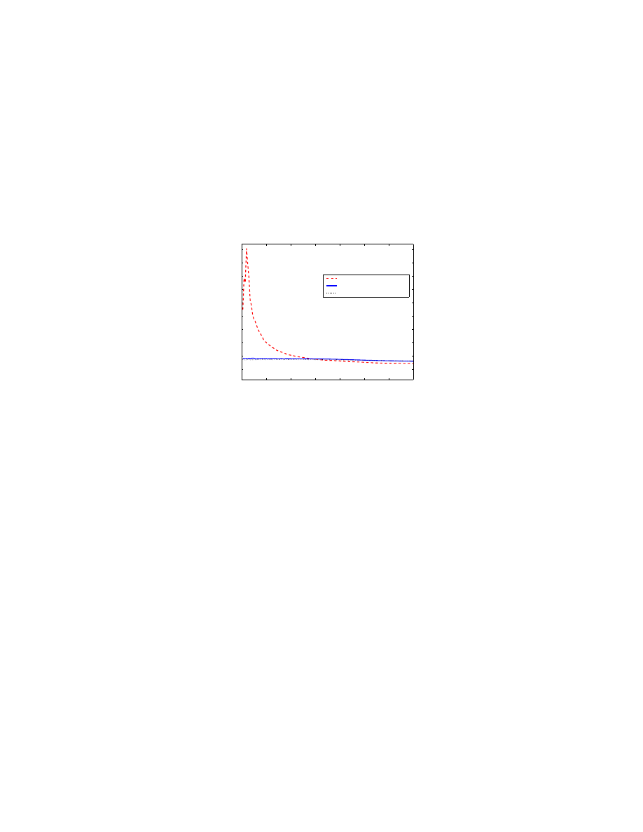
Fig. 11(a) shows that a power law topology has a selective percolation threshold (the threshold here

is about 0.29). If the fraction of users selectively immunized exceeds this threshold, the email network
will be broken into separated fragments and no virus outbreak will occur.

The selective percolation threshold of a power law topology is much smaller than that for either a

small world topology or a random graph topology. Although a power law topology is more vulnerable
under deliberate attacks [4], it benefits more from a selective immunization defense.

From Fig. 11(a) we can see that when we immunize the top 5% of most connected nodes in a power

law network, though 97.5% of remaining nodes in the network are still connected, 55.5% of the network
edges have been removed. Thus an email virus has fewer and longer paths to reach and infect nodes
in the remaining network. Fig. 11(b)(c) show that this is not the case for a small world topology or a
random graph topology, a 5% selective immunization removes fewer than 20% edges.

VI. C

ONCLUSION

In this paper we presented an email virus model by considering email users’ behaviors such as email

checking frequency and the probability to open an email attachment. We explained why we believe email
network can and should be modeled by a power law topology. We carried out extensive simulations of
email virus propagation and mathematically proved that the variability of email checking time affects virus
spreading speed. We also studied the effect of topology on virus propagation on power law, small world
and random graph topologies. From these simulation studies, we have derived a better understanding
of email virus’s behaviors and also the differences among power law, small world and random graph
topologies.

Compared to small world and random graph topologies, the impact of power law topology on email

virus is mixed: on the one hand, an email virus will spread faster on a power law topology than on a

16

small world or a random graph topology; on the other hand, it is more effective to carry out selective
immunization on a power law topology than on the other two topologies.

In this paper we mainly use simulation to study email virus propagation. The next step is to mathemati-

cally analyze email virus spreading. We also only considered a static immunization defense. In real email
virus propagation, some infected users will recover and develop an immunity to the email virus during
virus propagation. Thus in the real world, the immunization defense is a dynamic process. Considering
this dynamic process will give us more accurate modeling and prediction of email virus propagation. In
this paper we assume that the relationship of all email addresses is bi-directional, which may not be true
for some email users. In the future we need to consider directed graph for email network in order to get
a better picture of email virus propagation.

VII. A

CKNOWLEDGEMENT

This work was supported in part by DARPA under contract F30602-00-2-0554 and by NSF under

Grant EIA-0080119. It was also supported in part by ARO contract DAAD19-01-1-0610 and contract
2000-DT-CX-K001 from the U.S. Department of Justice, Office of Justice Programs.

The authors would like to thank Zihui Ge and Daniel R. Figueiredo for providing the size distribution

data of Yahoo! groups.

R

EFERENCES

[1] Tian Bu, Don Towsley. On Distingishing between Internet Power Law Topology Generators. Infocom, 2002.
[2] D. Watts, S. Strogatz. Collective dynamic of small-world networks. Nature, 393-400, 1998.
[3] R. Albert and A. Barabasi. Topology of Evolving Network: Local Events and Universality. Physica Review Letters, 85:5234-

5237, 2000.

[4] R. Albert, Hawoong Jeong and A. Barabasi. Error and attack tolerance of complex networks. nature, 378-382, 2000.
[5] Mihajlo A. Jovanovic Fred S. Annexstein, Kenneth A. Berman. Modeling Peer-to-Peer Network Topologies Through

“Small-World” Models and Power Laws. IX Telecommunications Forum, Belgrade,2001.

[6] J.O. Kephat and S.R. White. Directed-graph Epidemiological Models of Computer Viruses. Proc. 1991 IEEE Computer

Society Symposimum on Research in Security and Privacy, 343-359, 1991.

[7] J.O. Kephart, S.R. White and Chess. Computers and Epidemiology. IEEE Spectrum, May 1993.
[8] Jeffrey O. Kephart and Steve R. White. Measuring and Modeling Computer Virus Prevalence. Proc. 1993 IEEE Computer

Society Symposium on Research in Security and Privacy, Oakland, California, 1993.

[9] Wang, C., J.C. Knight, M. Elder. On Viral Propagation and the Effect of Immunization. Proc. 16th ACM Annual Computer

Applications Conference, New Orleans, LA Dec. 2000.

[10] Stuart Staniford, Vern Paxson and Nicholas Weaver. How to Own the Internet in Your Spare Time. Usenix Security, 2002.
[11] Yahoo! Groups. http://groups.yahoo.com
[12] Robert J. Adler, Raisa E. Feldman and Murad S. Taqqu. A practical guide to heavy tails : statistical techniques and

applications. Boston : Birkhuser, 1998.

[13] F. Cohen. Computer Viruses: Theory and Experiments. Computers & Security, Vol.6 22-35, 1987.
[14] P. Erd¨os, Graph theory and probability, Canad. J. Math., Vol.11, 34-38, 1959.
[15] C. Moore and M.E.J. Newman. Exact solution of site and bond percolation on small-world networks. Phys. Rev. E 62,

7059-7064, 2000.

[16] M.E.J. Newman, I. Jensen and R.M. Ziff. Percolation and epidemics in a two-dimensional small world. Phys. Rev. E 65,

2002.

[17] Eric Steen. The Case for an SMTP Gateway Anti-Virus System. http://rr.sans.org/email/SMTP.php
[18] legality of email monitoring. http://www.email-policy.com/#legal
[19] Melissa Virus’ Author Owns Up. CBS news. http://www.cbsnews.com/stories/1999/12/09/tech/

main73910.shtml

[20] Michele Masterson. Love bug costs billions. CNN news. http://money.cnn.com/2000/05/05/technology/virus impact
[21] CERT Advisory CA-1999-04 Melissa Macro Virus. http://www.cert.org/advisories/CA-1999-04.html
[22] Robert Lemos. SirCam worm still a serious threat. CNet news. http://news.com.com/2100-1001-272593.html?tag=bplst
[23] CERT Advisory CA-2001-22 W32/Sircam Malicious Code. http://www.cert.org/advisories/CA-2001-22.html
[24] 3rd Quarter 2001 - a nightmare for the security community and Internet users. Norman Security Information.

http://www.norman.no/security info/2001 41.shtml

17

[25] CERT Advisory CA-2000-04 Love Letter Worm. http://www.cert.org/advisories/CA-2000-04.html
[26] VBS.LoveLetter and variants. symantec security response. http://www.symantec.com/avcenter/venc/data/

vbs.loveletter.a.html

[27] CERT Advisory CA-2001-26 Nimda Worm. http://www.cert.org/advisories/CA-2001-26.html
[28] Clem Colman. Reflections on ”I Love You”. http://www.colmancomm.com/news/20000628ILY.htm
[29] CERT Advisory CA-2001-20 Continuing Threats to Home Users http://www.cert.org/advisories/CA-2001-20.html
[30] Sheldon M. Ross. Stochastic Processes. John Wiley & Sons, Inc. 1996.