Metoda przemieszczeń

1. Schemat podstawowy P

A B

1

φ₁ φ₁ -kąt rzeczywisty

Rys.1

2. Stan jednostkowy φ₁=1radian wywołujący reakcję utwierdzenia 1, pod postacią momentu K₁₁[Nm/1radian]

K₁₁

A B

1

φ₁=1

Z warunku równowagi momentów działających na węzeł 1 obliczamy K₁₁=M_1A+M_1B

K₁₁ +1

A 1 1 1 1 B

M_1A M_1B

1

+1 φ₁=1 Rys.1a

Na rysunku przedstawiono działanie momentów na węzeł 1 i jego oddziaływanie nie podano działania sił, które tam występują.

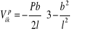
3. Reakcja podpory 1 od siły P

P K_1P

A B

1 Rys.1b

Po obciążeniu konstrukcji siłą P na nieruchome utwierdzenie 1 działa moment wywołany oddziaływaniem belki 1A. W tym przypadku, ponieważ belka 1B jest nie obciążona, jej oddziaływanie jest równe 0, stąd z warunku równowagi utwierdzenia 1
(rys.1c).

P K_1P

A 1 1 1 1 B

,

Rys.1c

4. Równanie kanoniczne
…………………………….……(1)

5. Stopień geometrycznej niewyznaczalności
…………….(2)

Gdzie
---liczba obrotów węzłów sztywnych

---liczba możliwych przesunięć węzłów

Stopień geometrycznej niewyznaczalności konstrukcji z rys.1:

,
,

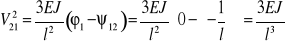
Wzory transformacyjne

1-wszy przypadek pręt obustronnie utwierdzony rys.2

EJ_ik

i k

ν_i l_ik

ν_k

i φ_k

ψ_ik

φ_i k

M_ik M_ki

i k Rys.2

V_ik V_ki

Z rys.1
…………………………………………(3)

Wzory transformacyjne

…………...(4)

………………(5)

2 -gi przypadek pręt jednym końcem utwierdzony drugim podpartym przegubowe rys.3

EJ_ik

i k

ν_i l_ik

ν_k

i x

ψ_ik ν(x)

k

φ_i

M_ik M_ki = 0

i k Rys.3

V_ik V_ki

Wzory transformacyjne

………………………………………………....(6)

…………………..(7)

3-ci przypadek pręt utwierdzony w k, w i podparty przegubowo (rys3a)

EJ_ik x

i k

ν_i l_ik

ν(x) ν_k

i φ_k

ψ_ki k k

M_ik = 0 M_ki

i k Rys.3a

V_ik V_ki

Wzory transformacyjne

………………………………………………….(6a)

,
………………….(7a)

Gdzie:
są reakcjami więzów od rzeczywistego obciążenia prętów.

Przykłady wartości tych reakcji dla kilku przypadków obciążenia prętów.

===========================================================

Przypadek 1a

P

i k

a b

Rys.4

,
;
,

M_x M_x

Wykres momentu M_x i siły tnącej T, dodatnie zwroty x

T T

+T

x

i a k

M_x=a

+M_x

Rys.5

Przypadek 1b………………………………………………………………………….

q

i l k

Rys.6

,
;
,

M_x M_x

Wykres momentu M_x i siły tnącej T, dodatnie zwroty x

T T

+T

k x

i l/2 -ql/2

M_x=l/2

+M_x

Rys.7

Przypadek 2a…………………………………………………………………………

P

i k

a b

Rys.8

,

,

M_x M_x

Wykres momentu M_x i siły tnącej T, dodatnie zwroty x

T T

+ T

i k x

a b

M_max

+ M_x

i k x

Rys.9

Przypadek 2b…………………………………………………………………………..

q

k

i l

Rys.6

,

,

M_x M_x

Wykres momentu M_x i siły tnącej T, dodatnie zwroty x

T T

+ T

i k x

0,625l

(M_max)₁

+ M_x l/4

i k x

M_max

Rys.10
,

==============================================================

Przykład 1

Dla konstrukcji przedstawionej na rys 11 sporządź wykres momentu gnącego i siły tnącej. Konstrukcja zbudowana jest z dwóch belek AB i BC o identycznej sztywności na zginanie połączonych przegubem B.

Dane:
, przekrój poprzeczny belki jest pełnym okręgiem o promieniu
, moduł Younga
, P=1000N, granica sprężystości materiału

, minimalny współczynnik bezpieczeństwa na zginanie n=2.

φ₁

A Δ₂ P B C

l l l

Rys.11

Rozwiązanie

Obliczenie stopnia geometrycznej niewyznaczalności z zależności (2)

, wniosek konstrukcja jest dwukrotnie geometrycznie niewyznaczalna.

Równania kanoniczne mają postać:

………………………………………………(a)

……………………………………………….(b)

Schemat podstawowy przedstawiono na rys.12

A 2 1 C

A 2 2 1 1 C

Rys.12

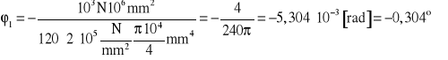
Równania równowagi momentów działających na utwierdzenie 1 (rys.13)

1

2 1 1 C

Rys.13

stąd (kolorowe reakcje prętów na utwierdzenie)

…………………..(c)

Równanie równowagi sił działających na wyciętą podporę 2 (rys.14)

2

A 2 2 1

K_2i

y Rys.14

, stąd (kolorowe reakcje prętów na utwierzenie)

………………………….(d)

Siły występujące w równaniach (c) i (d) obliczymy z równań (4)….(7)

Stan jednostkowy
(rys.15)

φ₁=1

A 2 1 C

l l l

Rys.15. Narysowane reakcje utwierdzenia na pręty

Siły na końcach pręta 2-1, przypadek 2, wzory (6) i (7),
(rys.3) ponieważ

………………………..(e)

………………………...(f)

………………………(f1)

Siły na końcach pręta 1-C, przypadek 1 wzory (4) i (5)
(rys.2) ponieważ

(rys.2) ponieważ

………….(g)

…………(h)

Podstawiając (e) i (g) do (c) oraz (f1) i (f) do (d) otrzymujemy

………………………………..(h1)

……………………………………....(h2)

Wykres momentu gnącego M₁ jest to moment który powstaje w układzie przy obrocie utwierdzenia 1 o kąt φ₁ = 1.(rys.16) M₁ M₁

Dodatnie zwroty momentu M₁ i siły tnącej T, x

T T

2

A C

1

l l l

+M₁

Rys.16

Stan jednostkowy
(rys.17)

,

A 2
1
C

ψ_2A Δ=1 +ψ₂₁

l
l l

Rys.17

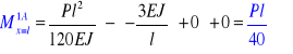
Siły na końcach pręta 1-A, przypadek 2 wzory (6) i (7)

,

(rys.3a)

………………………………...(i)

…………………………..…. (j)

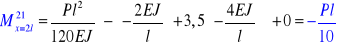
Siły na końcach pręta 2-1, przypadek 2,wzory wzory (6) i (7)

………………………………..(k)

………………………………..(l)

Wykres momentu M₂ rys.17a

A 2 1 C

+M₂ Rys.17a

Siły na końcach pręta 1-C rys.17

………………………(m)

Wstawiając (k) oraz (m) do (c) obliczamy reakcję K₁₂

…………………………………………….(n)

Porównując (n) z (h2) potwierdzamy że

Wstawiając (j) i (l) do (d) otrzymujemy

……………………………….(n1)

Stan p (i=1)odpowiadający rzeczywistemu obciążeniu układu rys.18

W stanie p nie deformuje się żaden pręt

Siły na końcach prętów są równe zeru, nie ma momentów M_p

P

A 2
1

C

l K_2p l l Rys.18

Zwroty sił i momentów przedstawione na rysunku 18 odpowiadają zwrotom oddziaływania podpory na pręty. Na rys.13 i rys.14 są oddziaływania prętów na podporę.

Reakcje obliczone z równań (c) i (d) mają wartości (rys.13 i rys.14).

Z warunku równowagi momentów węzła 1

………………………………………………(o)

Z warunku równowagi sił działających węzeł 2

………………….…………………..(p)

Po podstawieniu (h1), (h2), (n1), (o) i (p) do (a) i (b). Równania kanoniczne mają postać

1)
po skróceniu przez
,
stąd

2)

Po rozwiązaniu tego układu otrzymujemy poszukiwane niewiadome przemieszczenia

,
…………………………(r)

Moment gnący w prętach obliczamy ze wzoru

po podstawieniu (r)

…………………… …..(s)

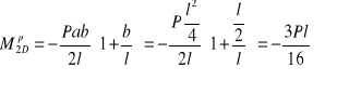
Obliczenia do wykresu M_x

1) Przekrój A ….

,
,

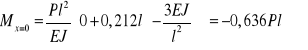
2) Przekrój węzeł 2

3) Przekrój 1 dla
od strony

4) Przekrój 1 dla
od strony

,
,

5) Przekrój C dla

,

Literatura. Rakowski G:. Mechanika budowli. Oficyna Wydawnicza WSEiZ, Warszawa

2004. Strona 123.

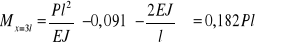
Wykres M_x przedstawiono na rys.19

- 0,636Pl -0,363Pl

A C x

M_x 2 1 0,182Pl

Rys.19 Wypadkowy moment gnący M_x

Wykresy sił tnących sporządzamy w następujący sposób

1. każdy z odcinków konstrukcji miedzy podporami traktujemy jako belkę podpartą swobodnie obciążoną na końcach momentami M_x. W naszym przypadku wartości te bierzemy z wykresu (rys.19).

2. dla każdego pręta obliczamy wartości reakcji podpór

3. znając wartości sił reakcji sporządzamy wykresy sił tnących.

Odcinek A2 (rys.20), wartości momentów
(rys.19)

T

l

A 2

Rys.20 T

Równanie równowagi momentów względem A

Odcinek 21 (rys.21), wartości momentów

T l

2 1

Rys.21

T

Równanie równowagi momentów względem 1

Odcinek 1C (rys.22), wartości momentów

T

l

1 C

T

Rys.22

Równanie równowagi momentów względem 1

Na rysunku 23 przedstawiono wykres sił tnących T w konstrukcji.

- 0,364P

0,636P 0,546P

T Rys.23

Obliczenie wartości maksymalnych naprężeń od zginania.

Wzór na naprężenia

, naprężenia maksymalne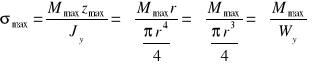

Z wykresu (rys.19) widać że M_max występuje w przekroju A i ma wartość

.

Wskaźnik wytrzymałości

Naprężenia od zginania

Minimalny współczynnik bezpieczeństwa n = 2

Rzeczywisty współczynnik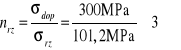

Wniosek: konstrukcja jest bezpieczna.

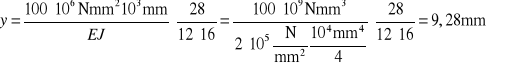
Obliczenie wartości przemieszczenia węzła 2 wzór (r)

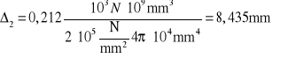
Węzeł 2 przemieści się w dół o wartość
.

Przykład 2

Dla konstrukcji przedstawionej na rys 24 sporządź wykres momentu gnącego i siły tnącej. Konstrukcja zbudowana jest z belki AD o sztywności na zginanie EJ = constans. Dane:
, przekrój poprzeczny belki jest pełnym okręgiem o promieniu
, moduł Younga
, P =1000N, granica sprężystości materiału

, minimalny współczynnik bezpieczeństwa na zginanie n=1.

φ₁ φ₂ P l/2

1 2

A D

l l l

Rys.24

Rozwiązanie

Obliczenie stopnia geometrycznej niewyznaczalności z zależności (2)

, wniosek konstrukcja jest dwukrotnie geometrycznie niewyznaczalna.

Równania kanoniczne mają postać:

………………………………………………(a*)

……………………………………………….(b*)

1. Schemat podstawowy przedstawiono na rys.25

1 2

A D

l l l

Rys.25

2. Stan jednostkowy φ₁=1, podano na rys.26

φ₁=1

1 2

A D

l l l

Rys.26

Równania równowagi momentów działających na utwierdzenie 1 (rys.27)

1

A 1 1 2

Rys.27

stąd (kolorowe reakcje prętów na utwierdzenie)

…………………..(c*)

Moment
obliczamy ze wzoru (4)

Moment
obliczamy ze wzoru (6a)

Podstawiając otrzymane wartości do (c*) otrzymujemy
…….(d*)

Równania równowagi momentów działających na utwierdzenie 2 (rys.28)

2

1 2 2 D

Rys.28

(kolorowe reakcje prętów na utwierdzenie) stąd

………………..(e*)

Moment
obliczamy ze wzoru (4)

Podstawiając otrzymaną wartość do (e*) otrzymujemy

Wykres momentu gnącego M₁ (rys.29) jest to moment który powstaje w układzie przy obrocie utwierdzenia 1 o kąt φ₁ = 1.(rys.26) M₁ M₁

Dodatnie zwroty momentu M₁ i siły tnącej T, x

T T

2

A D

1 2

l l l

+M₁

Rys.29

3. Stan jednostkowy φ₂=1, podano na rys.30

φ₂=1

1 2

A D

l l l

Rys.30

Równania równowagi momentów działających na utwierdzenie 2 (rys.27)

2

1 2 2 D

Rys.31

stąd (kolorowe reakcje prętów na utwierdzenie)

…………………..(f*)

Moment
obliczamy ze wzoru (4)

Moment
obliczamy ze wzoru (6)

Podstawiając otrzymane wartości do (f*) otrzymujemy
…….(g*)

Równania równowagi momentów działających na utwierdzenie 1 (rys.32)

1

A 1 1 2

Rys.32

(kolorowe reakcje prętów na utwierdzenie) stąd

………………..(h*)

Moment
obliczamy ze wzoru (4)

Podstawiając otrzymaną wartość do (h*) otrzymujemy

Wykres momentu gnącego M₂ (rys.33) jest to moment który powstaje w układzie przy obrocie utwierdzenia 2 o kąt φ₂ = 1.(rys.30) M₁ M₁

Dodatnie zwroty momentu M₂ i siły tnącej T, x

T T

1 2

A D

l l l

+M₂

Rys.33

4. Stan "p" stan w którym obliczamy siły i momenty wywołane obciążeniem zewnętrznym (rys.34)

,

P

2

A 1 1 2 2 D

Rys.34

Obliczenie wartości
z warunku równowagi węzła 1 (patrz rysunek 27)

Obliczenie wartości
z warunku równowagi węzła 2

Na rysunku 8 opisany jest przypadek 2a który odpowiada naszemu przypadkowi obciążenia występującemu na odcinku 2D stąd

,
,

Wykres momentu M_p jest przedstawiony na rys.35

-3Pl/16

A 1 2 D

+ M_p M_max

Rys.35 0,5l

wartość

Podstawiając otrzymane wartości do równań kanonicznych (a*), (b*) otrzymujemy

układ dwóch równań z dwoma niewiadomymi φ₁ i φ₂

po podzieleniu przez
otrzymujemy

po podzieleniu przez
i wstawieniu

otrzymujemy
gdzie

po podstawieniu danych

ponieważ
to

Sporządzenie wykresu rzeczywistego momentu M_x gnącego belkę AD (rys.36)

Wzór na M_x

po podstawieniu

Dla x = 0, M_x = 0

Dla x = l,

dla odcinka belki A1

Dla odcinka belki 12

Dla x = 2l

Dla odcinak belki 21

Dla odcinka 2D

Obliczenie wartości momentu dla

gdzie wartość (M_p)_max wzięto z przypadku 2a rys.9

Ponieważ w punkcie D istnieje przegub
, można to sprawdzić podstawiając

do (i*)

- 1,0 l/2

0 A 1

0,25 2 D

2,0 Rys.36

Maksymalny moment gnący belkę występuje w miejscu działania sił P i ma wartość

Obliczenie maksymalnych naprężeń od zginania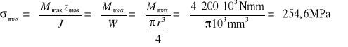

Współczynnik bezpieczeństwa w stosunku do granicy sprężystości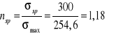
, warunek
został spełniony.

Wykresy sił tnących sporządzamy w następujący sposób

4. każdy z odcinków konstrukcji miedzy podporami traktujemy jako belkę podpartą swobodnie obciążoną na końcach momentami M_x i obciążeniem zewnętrznym. W naszym przypadku wartości M_x bierzemy z wykresu (rys.36).

5. dla każdego pręta obliczamy wartości reakcji podpór

6. znając wartości sił reakcji sporządzamy wykresy sił tnących.

Odcinek A1 (rys.37), wartości momentów
(rys.36)

T

l

A 1

T Rys.37

Równanie równowagi momentów względem A

Odcinek 12 (rys.38), wartości momentów
(rys.36)

T

l

1 2

T Rys.38

Równanie równowagi momentów względem 1

Odcinek 2D (rys.39), wartości momentów oraz obciążenia zewnętrznego P

(rys.36)

T_2P P

l/2

2 D

l Rys.39

y T

Z równania równowagi momentów względem 2 obliczam wartość T

Z warunku równowagi rzutu sił na oś y obliczam wartość siły

Wykres siły tnącej T

- 400

-125 A

0,25 1 2 l/2 D

600

T [N]

Rys.40

Przykład 3

Dla konstrukcji przedstawionej w przykładzie 2 obliczyć wartość ugięcia belki w miejscu działania siły P. Wartość ugięcia określić względem podpór 2 i D. Przy rozwiązaniu wykorzystać wartości momentów gnących przedstawionych na wykresie (rys.36).

Rozwiązanie

a) Z belki AD wycinamy odcinek 2D (rys.41) na który działa siła P. Odcinek ten traktujemy jako samodzielną konstrukcję na którą działają momenty gnące odciętych części konstrukcji.

b) Bekę 2D obciążamy w miejscu "pomiaru" ugięcia wirtualną pionową siłą równą 1N (rys.41).

c) Rysujemy wykres momentu gnącego
od obciążenia wirtualnego (rys.41)

d) Wartość ugięcia obliczamy ze wzoru Maxwella-Mohra

wartość całki obliczymy graficznie

Wykres momentu M_x

l = 1m

-100 l/2

2 D

100

(2/3)·200

200

M_x [Nm]

S_C 1[N] S_C

l/4 l/6 l/6

Rys.41. S_C środek ciężkości trójkąta

e) Dla przypomnienia obliczamy wartość kąta φ₂ ugięcia. Obliczenia prowadzimy za pomocą wzoru Maxwella-Mohra

wartość całki obliczymy analitycznie

Wykres momentu M_x na przęśle 2D przedstawiono na rys.42.

Dla

Dla

Wykres momentu wirtualnego podano na rys.42

Podstawiając wyrażenia na momenty do wzoru Maxwella-Mohra otrzymujemy

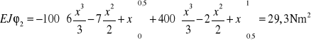
Wynik jest zgodny z tym co otrzymano rozwiązując układ równań kanonicznych

strona 18

l = 1m

-100 l/2

2 D

200

M_x [Nm]

1[Nm]

Rys.42. Wykres momentów rzeczywistego i wirtualnego

Odpowiedz:

Belka ugnie się o wartość y = 9,28mm, plus oznacza że ugięcie jest zgodne ze zwrotem obciążenia wirtualnego czyli do dołu.

3

---