
SG24-5415-00
International Technical Support Organization
www.redbooks.ibm.com
Getting Started with Data Warehouse
and Business Intelligence
Maria Sueli Almeida, Missao Ishikawa, Joerg Reinschmidt, Torsten Roeber


Getting Started with Data Warehouse
and Business Intelligence
August 1999
SG24-5415-00
International Technical Support Organization

© Copyright International Business Machines Corporation 1999.
All rights reserved
Note to U.S Government Users – Documentation related to restricted rights – Use, duplication or disclosure is
subject to restrictions set forth in GSA ADP Schedule Contract with IBM Corp.
First Edition (August 1999)
This edition applies to Version 5, Release 1of DB2 Server for VSE & VM Program Number 5648-158,
Version 5, Release 1of DB2 Server for OS/390 Program Number 5655-DB2, Version 5.2 of IBM Visual
Warehouse, Version 1.0.1 of IBM DB2 OLAP Server, Version 2.1.2 of IBM Intelligent Miner for Data,
Version 5.2 of IBM DB2 UDB for NT, Version 2.1.1of IBM DB2 DataJoiner Classic Connect, Version
2.1.3 of IBM DB2 Datajoiner for use with the Windows NT operating system, and Version 5.2 of IBM
DB2 UDB for AIX, Version 2.1.2 of IBM Intelligent MIner for Data, Version 2.1.3 of IBM DB2 DataJoiner,
Version 2.1.1 of IBM DB2 DataJoiner Classic Connect for use with the AIX Version 4.3.1 Operating
System, CrossAccess VSE V4.1.
Comments may be addressed to:
IBM Corporation, International Technical Support Organization
Dept. QXXE Building 80-E2
650 Harry Road
San Jose, California 95120-6099
When you send information to IBM, you grant IBM a non-exclusive right to use or distribute the
information in any way it believes appropriate without incurring any obligation to you.
Before using this information and the product it supports, be sure to read the general information in
Appendix B, “Special Notices” on page 225.
Take Note!

© Copyright IBM Corp. 1999
iii
Contents
Figures . . . . . . . . . . . . . . . . . . . . . . . . . . . . . . . . . . . . . . . . . . . . . . . . . . . vii
Tables. . . . . . . . . . . . . . . . . . . . . . . . . . . . . . . . . . . . . . . . . . . . . . . . . . . . .ix
Preface . . . . . . . . . . . . . . . . . . . . . . . . . . . . . . . . . . . . . . . . . . . . . . . . . . . .xi
The Team That Wrote This Redbook . . . . . . . . . . . . . . . . . . . . . . . . . . . . . . . . . xi
Comments Welcome . . . . . . . . . . . . . . . . . . . . . . . . . . . . . . . . . . . . . . . . . . . . xiii
Chapter 1. What is BI ? . . . . . . . . . . . . . . . . . . . . . . . . . . . . . . . . . . . . . . 1
1.1 The Evolution of Business Information Systems . . . . . . . . . . . . . . . . . . 1
1.1.1 First-Generation: Host-Based Query and Reporting . . . . . . . . . . . 1
1.1.2 Second-Generation: Data Warehousing . . . . . . . . . . . . . . . . . . . . 2
1.1.3 Third-Generation: Business Intelligence . . . . . . . . . . . . . . . . . . . . 2
1.2 Why Do You Need Business Intelligence ? . . . . . . . . . . . . . . . . . . . . . . 5
1.3 What Do You Need for Business Intelligence ? . . . . . . . . . . . . . . . . . . 5
1.4 Business Driving Forces . . . . . . . . . . . . . . . . . . . . . . . . . . . . . . . . . . . . 7
1.5 Business Intelligence Requirements . . . . . . . . . . . . . . . . . . . . . . . . . . . 8
1.6 The IBM Business Intelligence Product Set . . . . . . . . . . . . . . . . . . . . . 8
1.6.1 Business Intelligence Applications . . . . . . . . . . . . . . . . . . . . . . . . 9
1.6.2 Decision Support Tools. . . . . . . . . . . . . . . . . . . . . . . . . . . . . . . . 10
1.7 The Challenge of Data Diversity . . . . . . . . . . . . . . . . . . . . . . . . . . . . . 14
Chapter 2. ITSO Scenario . . . . . . . . . . . . . . . . . . . . . . . . . . . . . . . . . . . 17
2.1 The Environment . . . . . . . . . . . . . . . . . . . . . . . . . . . . . . . . . . . . . . . . 17
2.1.1 Database Server . . . . . . . . . . . . . . . . . . . . . . . . . . . . . . . . . . . . 18
2.1.2 Visual Warehouse . . . . . . . . . . . . . . . . . . . . . . . . . . . . . . . . . . . 19
2.1.3 Communication Gateways . . . . . . . . . . . . . . . . . . . . . . . . . . . . . 19
2.1.4 Data Analysis Tools . . . . . . . . . . . . . . . . . . . . . . . . . . . . . . . . . . 20
2.2.1 Sales Information . . . . . . . . . . . . . . . . . . . . . . . . . . . . . . . . . . . . 21
2.2.2 Article Information . . . . . . . . . . . . . . . . . . . . . . . . . . . . . . . . . . . 21
2.2.3 Organization Information . . . . . . . . . . . . . . . . . . . . . . . . . . . . . . 23
2.3 Data Warehouse for OLAP . . . . . . . . . . . . . . . . . . . . . . . . . . . . . . . . . 24
Chapter 3. The Products and Their Construction . . . . . . . . . . . . . . . . . 29
3.1 The DataJoiner Product . . . . . . . . . . . . . . . . . . . . . . . . . . . . . . . . . . . 29
3.1.1 DataJoiner Classic Connect Component. . . . . . . . . . . . . . . . . . . 29
3.1.2 DataJoiner Classic Connect Architecture . . . . . . . . . . . . . . . . . . 30
3.2.1 CrossAccess Architecture. . . . . . . . . . . . . . . . . . . . . . . . . . . . . . 36
3.3 Visual Warehouse: Server and Agent . . . . . . . . . . . . . . . . . . . . . . . . . 42

iv
Getting Started with Data Warehouse and Business Intelligence
3.3.1 Data Sources Supported . . . . . . . . . . . . . . . . . . . . . . . . . . . . . . 42
3.3.2 Data Stores Supported . . . . . . . . . . . . . . . . . . . . . . . . . . . . . . . . 42
3.3.3 End User Query Tools . . . . . . . . . . . . . . . . . . . . . . . . . . . . . . . . 43
3.3.4 Meta Data Management . . . . . . . . . . . . . . . . . . . . . . . . . . . . . . . 43
3.3.5 The Architecture of Visual Warehouse . . . . . . . . . . . . . . . . . . . . 43
3.4.1 Overview of the Intelligent Miner. . . . . . . . . . . . . . . . . . . . . . . . . 45
3.4.2 Working with Databases . . . . . . . . . . . . . . . . . . . . . . . . . . . . . . . 45
3.4.3 The User Interface . . . . . . . . . . . . . . . . . . . . . . . . . . . . . . . . . . . 46
3.4.4 Data Preparation Functions . . . . . . . . . . . . . . . . . . . . . . . . . . . . 46
3.4.5 Statistical and Mining Functions . . . . . . . . . . . . . . . . . . . . . . . . . 47
3.4.6 Processing IM Functions . . . . . . . . . . . . . . . . . . . . . . . . . . . . . . 48
3.4.7 Creating and Visualizing the Results . . . . . . . . . . . . . . . . . . . . . 49
3.4.8 Creating Data Mining Operations . . . . . . . . . . . . . . . . . . . . . . . . 50
3.5 DB2 OLAP Server . . . . . . . . . . . . . . . . . . . . . . . . . . . . . . . . . . . . . . . 51
3.5.1 The General Architecture . . . . . . . . . . . . . . . . . . . . . . . . . . . . . . 53
3.5.2 Architecture and Concepts of DB2 OLAP Server and Essbase . . 53
3.5.3 Supported Platforms and RDBMSs . . . . . . . . . . . . . . . . . . . . . . . 57
3.5.4 Wired for OLAP Server . . . . . . . . . . . . . . . . . . . . . . . . . . . . . . . . 57
3.6 DB2 Connect . . . . . . . . . . . . . . . . . . . . . . . . . . . . . . . . . . . . . . . . . . . 58
3.7 IBM e-Network Communication Server Host-on Demand . . . . . . . . . . 65
3.7.1 Communication Server . . . . . . . . . . . . . . . . . . . . . . . . . . . . . . . . 65
3.7.2 Host-on Demand . . . . . . . . . . . . . . . . . . . . . . . . . . . . . . . . . . . . 70
3.8 Net.Data and Its Architecture . . . . . . . . . . . . . . . . . . . . . . . . . . . . . . . 72
3.9 Web Server . . . . . . . . . . . . . . . . . . . . . . . . . . . . . . . . . . . . . . . . . . . . 74
Chapter 4. Data Communication . . . . . . . . . . . . . . . . . . . . . . . . . . . . . . 77
4.1 Communication Protocols . . . . . . . . . . . . . . . . . . . . . . . . . . . . . . . . . . 78
4.1.1 TCP/IP . . . . . . . . . . . . . . . . . . . . . . . . . . . . . . . . . . . . . . . . . . . . 78
4.1.2 APPC . . . . . . . . . . . . . . . . . . . . . . . . . . . . . . . . . . . . . . . . . . . . . 89
4.2 Data Exchange Protocols . . . . . . . . . . . . . . . . . . . . . . . . . . . . . . . . . 96
4.2.1 DRDA Remote Unit of Work (RUW) . . . . . . . . . . . . . . . . . . . . . . 96
4.2.2 DRDA Distributed Unit of Work (DUW) . . . . . . . . . . . . . . . . . . . . 96
4.2.3 Distributed Request (DR) . . . . . . . . . . . . . . . . . . . . . . . . . . . . . . 97
4.2.4 Private Protocols . . . . . . . . . . . . . . . . . . . . . . . . . . . . . . . . . . . . 97
4.2.5 Nonrelational Access . . . . . . . . . . . . . . . . . . . . . . . . . . . . . . . . . 97
Chapter 5. Implementation . . . . . . . . . . . . . . . . . . . . . . . . . . . . . . . . . . 99
5.1 OS/390 Environment . . . . . . . . . . . . . . . . . . . . . . . . . . . . . . . . . . . . . 99
5.1.1 IMS/ESA Environment Configuration . . . . . . . . . . . . . . . . . . . . . 99
5.1.2 DataJoiner Classic Connect Configuration . . . . . . . . . . . . . . . . 100
5.1.3 Network Communication Protocol Configurations . . . . . . . . . . . 102
5.1.4 Configuring Data Server Communications on OS/390. . . . . . . . 104

v
5.1.5 Configuring an AIX Classic Connect Client . . . . . . . . . . . . . . . . 106
5.1.6 Mapping Non-Relational Data (VSAM) . . . . . . . . . . . . . . . . . . . 107
5.1.7 Mapping Non-Relational Data (IMS) . . . . . . . . . . . . . . . . . . . . . 115
5.1.8 DataJoiner Connectivity . . . . . . . . . . . . . . . . . . . . . . . . . . . . . . 123
5.1.9 Accessing Your Data . . . . . . . . . . . . . . . . . . . . . . . . . . . . . . . . 127
5.2.1 Installation . . . . . . . . . . . . . . . . . . . . . . . . . . . . . . . . . . . . . . . . 130
5.2.2 Product Installation and Configuration . . . . . . . . . . . . . . . . . . . 132
Chapter 6. The Data Warehouse Definitions . . . . . . . . . . . . . . . . . . . . 167
6.1 The Data Acquisition Process. . . . . . . . . . . . . . . . . . . . . . . . . . . . . . 167
6.1.1 The First Dimension . . . . . . . . . . . . . . . . . . . . . . . . . . . . . . . . . 167
6.1.2 The Second Dimension . . . . . . . . . . . . . . . . . . . . . . . . . . . . . . 170
6.2 Technical Implementation of the Data Acquisition Process . . . . . . . . 174
Appendix A. The OS/390 Environment . . . . . . . . . . . . . . . . . . . . . . . . . . 177
A.1 The IMS - DBCTL Environment . . . . . . . . . . . . . . . . . . . . . . . . . . . . . . . 177
A.2 The DB/DC Environment . . . . . . . . . . . . . . . . . . . . . . . . . . . . . . . . . . . . 178
A.3 Configuring the DBCTL Environment . . . . . . . . . . . . . . . . . . . . . . . . . . . 179
A.3.1 Create Stage 1 Input for DBCTL System . . . . . . . . . . . . . . . . . . . . 179
A.3.2 Run the IMS System Definition STAGE 1. . . . . . . . . . . . . . . . . . . . 182
A.3.3 Run the IMS System Definition STAGE 2. . . . . . . . . . . . . . . . . . . . 184
A.3.4 Create DFSPBxxx Member . . . . . . . . . . . . . . . . . . . . . . . . . . . . . . 184
A.3.5 Create IMS DBCTL Started Procedure. . . . . . . . . . . . . . . . . . . . . . 186
A.3.6 Create IMS DL/I Started Procedure . . . . . . . . . . . . . . . . . . . . . . . . 191
A.3.7 Create IMS DBRC Started Procedure . . . . . . . . . . . . . . . . . . . . . . 192
A.3.8 Allocate RECON Data Sets . . . . . . . . . . . . . . . . . . . . . . . . . . . . . . 194
A.3.9 Register DBRC Information . . . . . . . . . . . . . . . . . . . . . . . . . . . . . . 196
A.4.1 IMS Definitions . . . . . . . . . . . . . . . . . . . . . . . . . . . . . . . . . . . . . . . . 199
A.4.2 DB2 Definitions . . . . . . . . . . . . . . . . . . . . . . . . . . . . . . . . . . . . . . . . 204
A.4.3 VSAM Definitions . . . . . . . . . . . . . . . . . . . . . . . . . . . . . . . . . . . . . . 214
A.4.4 Classic Connect Definitions . . . . . . . . . . . . . . . . . . . . . . . . . . . . . . 216
A.5.1 TCP/IP for MVS Environment Setup. . . . . . . . . . . . . . . . . . . . . . . . 223
A.5.2 IMS Environment Setup . . . . . . . . . . . . . . . . . . . . . . . . . . . . . . . . . 223
A.5.3 Classic Connect Setup (for Data Server) . . . . . . . . . . . . . . . . . . . . 223
A.5.4 Classic Connect Setup (for Client) . . . . . . . . . . . . . . . . . . . . . . . . . 224
Appendix B. Special Notices . . . . . . . . . . . . . . . . . . . . . . . . . . . . . . . . . . 225
Appendix C. Related Publications. . . . . . . . . . . . . . . . . . . . . . . . . . . . . . 229
C.1 International Technical Support Organization Publications . . . . . . . . . . 229
C.2 Redbooks on CD-ROMs . . . . . . . . . . . . . . . . . . . . . . . . . . . . . . . . . . . . . 230

vi
Getting Started with Data Warehouse and Business Intelligence
How to Get ITSO Redbooks . . . . . . . . . . . . . . . . . . . . . . . . . . . . . . . . . 233
IBM Redbook Fax Order Form . . . . . . . . . . . . . . . . . . . . . . . . . . . . . . . . . . . . 234
List of Abbreviations. . . . . . . . . . . . . . . . . . . . . . . . . . . . . . . . . . . . . . . 235
Index . . . . . . . . . . . . . . . . . . . . . . . . . . . . . . . . . . . . . . . . . . . . . . . . . . . 239
ITSO Redbook Evaluation . . . . . . . . . . . . . . . . . . . . . . . . . . . . . . . . . . . 243

© Copyright IBM Corp. 1999
vii
Figures
IBM Business Intelligence Structure . . . . . . . . . . . . . . . . . . . . . . . . . . . . . . 4
IBM Business Intelligence Product Set . . . . . . . . . . . . . . . . . . . . . . . . . . . . 9
Classic Connect Architecture with Enterprise Server . . . . . . . . . . . . . . . . 34
CrossAccess Architecture with Enterprise Server . . . . . . . . . . . . . . . . . . . 40
CrossAccess Data Mapper Workflow . . . . . . . . . . . . . . . . . . . . . . . . . . . . 41
10. Sample Clustering Visualization . . . . . . . . . . . . . . . . . . . . . . . . . . . . . . . . 50
11. Sequence-Settings Window. . . . . . . . . . . . . . . . . . . . . . . . . . . . . . . . . . . . 51
12. Architecture Building Blocks of an OLAP Solution. . . . . . . . . . . . . . . . . . . 53
13. Hyperion Essbase and DB2 OLAP Server Architectures. . . . . . . . . . . . . . 56
14. DB2 Connect Enterprise Edition . . . . . . . . . . . . . . . . . . . . . . . . . . . . . . . . 59
15. DB2 Connect Personal Edition . . . . . . . . . . . . . . . . . . . . . . . . . . . . . . . . . 60
16. Net.Data Architecture . . . . . . . . . . . . . . . . . . . . . . . . . . . . . . . . . . . . . 74
17. TCP/IP Architecture Model: Layers and Protocols. . . . . . . . . . . . . . . . . . . 80
18. Assigned Classes of IP Addresses . . . . . . . . . . . . . . . . . . . . . . . . . . . . . . 81
19. Class A Address without Subnets . . . . . . . . . . . . . . . . . . . . . . . . . . . . . . . 83
20. Class A Address with Subnet Mask and Subnet Address . . . . . . . . . . . . . 84
21. Format of an IP Datagram Header. . . . . . . . . . . . . . . . . . . . . . . . . . . . 86
22. Direct and Indirect Routing . . . . . . . . . . . . . . . . . . . . . . . . . . . . . . . . . . . . 87
23. Routing Table Scenario . . . . . . . . . . . . . . . . . . . . . . . . . . . . . . . . . . . . . . . 88
24. IP Routing Table Entries Example . . . . . . . . . . . . . . . . . . . . . . . . . . . . . . . 88
25. IP Routing Algorithm (with Subnets) . . . . . . . . . . . . . . . . . . . . . . . . . . . . . 89
26. TCP/IP Communications Template and Worksheet . . . . . . . . . . . . . . . . 104
27. Relationship of DJCC Parameters . . . . . . . . . . . . . . . . . . . . . . . . . . . . . . 105
28. Example of Classic Connect Configuration file, djxclassic2.cfg . . . . . . . . 106
29. Example of .profile . . . . . . . . . . . . . . . . . . . . . . . . . . . . . . . . . . . . . . . . . . 107
30. Example of db2profile . . . . . . . . . . . . . . . . . . . . . . . . . . . . . . . . . . . . . . . 107
31. Output of JOBLOG for JDXDRA . . . . . . . . . . . . . . . . . . . . . . . . . . . . . . . 127
32. Result of ’db2 -vtf orgstruc.sql’. . . . . . . . . . . . . . . . . . . . . . . . . . . . . . . . . 128
33. Result of ’db2 -vtf firdb.sql’. . . . . . . . . . . . . . . . . . . . . . . . . . . . . . . . . . . . 129
34. Result of ’db2 -vtf filstam.sql’ . . . . . . . . . . . . . . . . . . . . . . . . . . . . . . . . . . 129
35. Sources for Dimension Table PRODUCT . . . . . . . . . . . . . . . . . . . . . . . . 168
36. Dimension Table PRODUCT from Join of Intermediate Sources . . . . . . 170
37. Sources for Dimension Table ORGANIZATION . . . . . . . . . . . . . . . . . . . 172
38. Dimension Table ORGANIZATION from JOIN of Intermediate Sources . 173
39. Example of a DBCTL Environment . . . . . . . . . . . . . . . . . . . . . . . . . . . . . 178
40. Example of a DB/DC Environment. . . . . . . . . . . . . . . . . . . . . . . . . . . . . . 179

viii
Getting Started with Data Warehouse and Business Intelligence
41. Example of DBD and PSB Specifications . . . . . . . . . . . . . . . . . . . . . . . . 180
42. Example of DFSPBxxx. . . . . . . . . . . . . . . . . . . . . . . . . . . . . . . . . . . . . . . 184
43. Example of IMS Started Procedure Parameter . . . . . . . . . . . . . . . . . . . . 186
44. Example of RECON Records Registration . . . . . . . . . . . . . . . . . . . . . . . 197

© Copyright IBM Corp. 1999
ix
Tables
DB2 Tables on SC19M . . . . . . . . . . . . . . . . . . . . . . . . . . . . . . . . . . . . . . . 24
DL/I ’Tables’ derived through CrossAccess . . . . . . . . . . . . . . . . . . . . . . . . 26
VSAM ’Tables’ derived through CrossAccess . . . . . . . . . . . . . . . . . . . . . . 27
DB2 Table in Windows NT database SJNTADD . . . . . . . . . . . . . . . . . . . . 27
VSE User IDs and ICCF Libraries . . . . . . . . . . . . . . . . . . . . . . . . . . . . . . 130
VSE Partition Allocation and Usage. . . . . . . . . . . . . . . . . . . . . . . . . . . . . 131
VTAM Configuration Members. . . . . . . . . . . . . . . . . . . . . . . . . . . . . . . . . 133
Table-Dbspace-Pool Relation . . . . . . . . . . . . . . . . . . . . . . . . . . . . . . . . . 154

x
Getting Started with Data Warehouse and Business Intelligence

© Copyright IBM Corp. 1999
xi
Preface
This redbook describes an operating environment that supports Data
Warehousing and BI solutions on all available platforms. The book describes
how this environment was established. This project was carried out at the
ITSO San Jose Center. DRDA over TCP/IP, DataJoiner Classic Connect,
Cross Access for VSE, and Datajoiner are used to create this environment.
The objective of creating this environment was to have a base BI environment
to support Data Warehouse, OLAP, and Data Mining solutions. This book is
not intended to show how to set up and configure the different products used;
some of these have been covered in previous product-specific redbooks.
This redbook is intended to be used in conjunction with the redbooks:
Intelligent Miner for Data: Enhance Your Business Intelligence, SG24-5422
and My Mother Thinks I'm a DBA! Cross-Platform, Multi-Vendor, Distributed
Relational Data Replication with IBM DB2 DataPropagator and IBM DataJoiner
Made Easy!, SG24-5463. Future redbooks will enhance and exploit this
environment.
The Team That Wrote This Redbook
This redbook was produced by a team of specialists from around the world
working at the International Technical Support Organization San Jose Center.
Maria Sueli Almeida is a Certified I/T Specialist - Systems Enterprise Data,
and is currently a specialist in DB2 for OS/390 and Distributed Relational
Database System (DRDS) at the International Technical Support
Organization, San Jose Center. Before joining the ITSO in 1998, Maria Sueli
worked at IBM Brazil assisting customers and IBM technical professionals on
DB2, data sharing, database design, performance, and DRDA connectivity.
Missao Ishikawa is an Advisory I/T Specialist, supporting Intelligent Miner
for OS/390 and Domino for S/390 in IBM Japan. He joined IBM in 1987 and
has been working in various areas of technical support. He has worked for
1998 Nagano Olympics as a DB2 specialist, supporting all aspects of DB2 for
OS/390.
Joerg Reinschmidt is an Information Mining Specialist at the International
Technical Support Organization, San Jose Center. He writes extensively and
teaches IBM classes worldwide on all areas of DB2 Universal Database,
Internet access to legacy data, Information Mining, and Knowledge
Management. Before joining the ITSO in 1998, Joerg worked in the Solution

xii
Getting Started with Data Warehouse and Business Intelligence
Partnership Center in Germany as a DB2 Specialist, supporting independent
software vendors (ISVs) to port their applications to use the IBM data
management products.
Torsten Roeber is a Software Service Specialist with IBM Germany. He has
several years of experience with VSE/ESA and DB2 (SQL/DS) for VSE and
VM. During the last two years he has focused on distributed database issues
in the VM/VSE and workstation environment.
Thanks to the following people for their invaluable contributions to this project:
Paolo Bruni
International Technical Support Organization, San Jose Center
Scott Chen
International Technical Support Organization, San Jose Center
Thomas Groh
International Technical Support Organization, San Jose Center
Rick Long
International Technical Support Organization, San Jose Center
Wiliam Tomio Kanegae
IBM Brazil
Wilhelm Mild
IBM Germany
Thanks also to the professionals from Cross Access Corporation, for
supporting and writing about the CrossAccess product.

xiii
Comments Welcome
Your comments are important to us!
We want our redbooks to be as helpful as possible. Please send us your
comments about this or other redbooks in one of the following ways:
• Fax the evaluation form found in “ITSO Redbook Evaluation” on page 243
to the fax number shown on the form.
• Use the electronic evaluation form found on the Redbooks Web sites:
For Internet users
http://www.redbooks.ibm.com/
For IBM Intranet users
http://w3.itso.ibm.com
• Send us a note at the following address:
redbook@us.ibm.com

xiv
Getting Started with Data Warehouse and Business Intelligence

© Copyright IBM Corp. 1999
1
Chapter 1. What is BI ?
When reading about business intelligence (BI), one of the global definitions
you may see is the one found on the IBM Business Intelligence Web page:
"Business intelligence means using your data assets to make better
business decisions. It is about access, analysis, and uncovering new
opportunities."
Many of the concepts of business intelligence are not new, but have evolved
and been refined based on experience gained from early host-based
corporate information systems, and more recently, from data warehousing
applications.
Given the increasing competition in today’s tough business climate, it is vital
that organizations provide cost-effective and rapid access to business
information for a wide range of business users, if these organizations are to
survive into the new millennium. The solution to this issue is a business
intelligence system, which provides a set of technologies and products for
supplying users with the information they need to answer business questions,
and make tactical and strategic business decisions.
1.1 The Evolution of Business Information Systems
Inevitably the first question that arises when describing the objectives of a
business intelligence system is, "Does a data warehouse have the same
objectives and provide the same capabilities as a business intelligence
system?" A similar question arose when data warehouses were first
introduced, "Is a data warehouse similar to the corporate information systems
and information centers we built in the past?" Although a quick and simple
answer to both questions is "yes", closer examination shows that, just as
there are important differences between a warehouse and early corporate
information systems and information centers, there are also important
differences between a business intelligence system and a data warehouse.
1.1.1 First-Generation: Host-Based Query and Reporting
Early business information systems employed batch applications to provide
business users with the information they needed. The output from these
applications typically involved huge volumes of paper that users had to wade
through to get the answers they needed to business questions. The advent of
terminal-driven time-sharing applications provided more rapid access to
information, but these systems were still cumbersome to use, and required
access to complex operational databases.

2
Getting Started with Data Warehouse and Business Intelligence
This first generation of business information systems could, therefore, only be
used by information providers, such as business analysts, who had an
intimate knowledge of the data and extensive computer experience.
Information consumers, like business executives and business managers,
could rarely use these early systems, and instead had to rely on information
providers to answer their questions and supply them with the information they
needed.
1.1.2 Second-Generation: Data Warehousing
The second generation of business information systems came with data
warehousing, which provided a giant leap forward in capability. Data
warehouses have several advantages over first-generation systems:
• Data warehouses are designed to satisfy the needs of business users and
not day-to-day operational applications.
• Data warehouse information is clean and consistent, and is stored in a
form business users can understand.
• Unlike operational systems, which contain only detailed current data, the
data warehouses can supply both historical and summarized information.
• The use of client/server computing provides data warehouse users with
improved user interfaces and more powerful decision support tools.
1.1.3 Third-Generation: Business Intelligence
A data warehouse is still not a complete solution to the needs of business
users. One weakness of many data warehouse solutions is that the vendors
often focus on technology, rather than business solutions. While there is no
doubt that data warehouse vendors provide powerful products for building
and accessing a data warehouse, these products can require a significant
amount of implementation effort.
The issue here is that warehouse products rarely come prepackaged for
specific industries or application areas, or address particular business
problems. This is very much like the situation in the early days of client/server
computing, when vendors initially provided the technology for developing
operational applications, but then quickly realized that organizations were
looking for application and business solutions, and not yet more technology.
Vendors fixed this problem, with the result that today many operational
client/server applications are built using application packages, rather than
being handcrafted by developers.

What is BI ?
3
The same evolution has to happen in business information systems – vendors
must provide application packages, and not just more technology. One
distinguishing factor of business intelligence systems is that they focus on
providing prepackaged application solutions in addition to improved
technology.
Another issue with data warehousing is that much of the focus is still on
building the data warehouse, rather than accessing it. Many organizations
seem to think that if they build a data warehouse and provide users with the
right tools, the job is done. In fact, it is just beginning. Unless the information
in the warehouse is thoroughly documented and easy to access, complexity
will limit warehouse usage to the same information providers as
first-generation systems.
Business intelligence systems focus on improving the access and delivery of
business information to both information providers and information
consumers. They achieve this by providing advanced graphical- and
Web-based online analytical processing (OLAP) and information mining tools,
and prepackaged applications that exploit the power of those tools. These
applications may need to process and analyze large volumes of information
using a variety of different tools. A business intelligence system must,
therefore, provide scalability and be able to support and integrate products
from multiple vendors.
A business intelligence system may also simplify access to business
information through the use an information catalog that documents decision
support objects that can be employed by information consumers to answer
the main business questions that arise in everyday business operations.
Some also reduce the need for information consumers to access the
warehouse at all. Instead, information consumers subscribe to the
information they require, and the system delivers it to them at predefined
intervals through a corporate intranet or e-mail.
The information stored in a data warehouse is typically sourced from
operational databases (and in some cases external information providers).
There is, however, also a considerable amount of business information kept in
office and workgroup systems, on Web servers on corporate intranets and the
public Internet, and in paper form on people’s desks. To solve this issue,
business intelligence systems are designed to support access to all forms of
business information, not only the data stored in a data warehouse. Having a
business intelligence system does not negate the need for a data warehouse
– a data warehouse is simply one of the data sources that can be handled by
a business intelligence system.
4
Getting Started with Data Warehouse and Business Intelligence
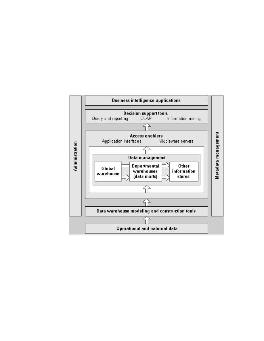
We see, then, that a business intelligence system is a third-generation
business information system that has three key advantages:
1. Business intelligence systems not only support the latest information
technologies, but also provide prepackaged application solutions.
2. Business intelligence systems focus on the access and delivery of
business information to end users, and support both information providers
and information consumers.
3. Business intelligence systems support access to all forms of business
information, and not just the information stored in a data warehouse.
Figure 1 gives an overall view of the IBM business intelligence structure.
Figure 1. IBM Business Intelligence Structure

What is BI ?
5
1.2 Why Do You Need Business Intelligence ?
Businesses collect large quantities of data in their day-to-day operations: data
about orders, inventory, accounts payable, point-of-sale transactions, and of
course, customers. In addition, businesses often acquire data, such as
demographics and mailing lists, from outside sources. Being able to
consolidate and analyze this data for better business decisions can often lead
to a competitive advantage, and learning to uncover and leverage those
advantages is what business intelligence is all about.
Some examples are:
• Achieving growth in sales, reduction in operating costs, and improved
supply management and development.
• Using OLAP to reduce the burden on the IT staff, improve information
access for business processing, uncover new sources of revenue, and
improve allocation of costs.
• Using data mining to extract key purchase behaviors from customer
survey data. NBA Coaches use IBM's Advance Scout to analyze game
situations and gain a competitive advantage over other teams.
All of this is possible if you have the right applications and tools to analyze
data, and more importantly, if the data is prepared in a format suitable for
analysis. For a business person, it is most important to have applications and
tools for data analysis, while for the IT community, having the tools to build
and manage the environment for business intelligence is key.
1.3 What Do You Need for Business Intelligence ?
Business decision-makers have vastly different levels of expertise, and
different needs for data analysis.
A wide range of approaches and tools are available, to meet their varied
needs:
• Applications such as IBM's DecisionEdge for customer relationship
management, and IBM's Business Discovery Series for data mining
• Query tools such as Impromptu and PowerPlay from Cognos,
BusinessObjects from Business Objects, Approach from Lotus
Development Corp., and IBM's Query Management Facility

6
Getting Started with Data Warehouse and Business Intelligence
• OLAP tools for multidimensional analysis such as Essbase from Arbor
Software, and IBM's DB2 OLAP Server (developed in conjunction with
Arbor)
• Statistical analysis tools such as the SAS System from SAS Institute Inc.
• Data Mining tools such as IBM's Intelligent Miner
Many of these applications and tools feature built-in support for Web
browsers and Lotus Notes, enabling users to get the information they need
from within a familiar desktop environment.
Most businesses do not want informal access to their operational computer
systems, either for security or performance reasons. Rather, they prefer to
build a separate system for business intelligence applications. To build these
systems, tools are needed to extract, cleanse, and transform data from
source systems which may be on a variety of hardware platforms, using a
variety of databases. Once the data is prepared for business intelligence
applications, the data is stored in a database system and must be refreshed
and managed. These systems are called data warehouses or data marts, and
the process of building and maintaining them is called data warehouse or
data mart generation and management.
IBM's principal solution for generating and managing these systems is Visual
Warehouse. Other IBM offerings such as the Data Replication Family and
DataJoiner (for multi-vendor database access) can complement Visual
Warehouse as data is moved from source to target systems. IBM also
partners with companies such as Evolutionary Technologies International for
more complex extract capabilities and Vality Technology Inc. for data
cleansing technology.
For the warehouse database, IBM offers the industry leader: DB2. The DB2
family spans AS/400 systems, RISC System/6000 hardware, IBM
mainframes, non-IBM machines from Hewlett-Packard and Sun
Microsystems, and operating systems such as OS/2, Windows (95 & NT),
AIX, HP-UX, SINIX, SCO OpenServer, and Solaris Operating Environment.
When DataJoiner is used in conjunction with Visual Warehouse, non-IBM
databases such as those from Oracle, Sybase, and Informix can be used as
the warehouse database.

What is BI ?
7
1.4 Business Driving Forces
So far we have seen that many of the driving forces behind business
intelligence come from the need to improve ease-of-use and reduce the
resources required to implement and use new information technologies.
There are, however, three additional important business driving forces behind
business intelligence:
1. The need to increase revenues, reduce costs, and compete more
effectively. Gone are the days when end users could manage and plan
business operations using monthly batch reports, and IT organizations
had months to implement new applications. Today companies need to
deploy informational applications rapidly, and provide business users with
easy and fast access to business information that reflects the rapidly
changing business environment. Business intelligence systems are
focused towards end-user information access and delivery, and provide
packaged business solutions in addition to supporting the sophisticated
information technologies required for the processing of today’s business
information.
2. The need to manage and model the complexity of today’s business
environment. Corporate mergers and deregulation means that companies
today are providing and supporting a wider range of products and services
to a broader and more diverse audience than ever before. Understanding
and managing such a complex business environment and maximizing
business investment is becoming increasingly more difficult. Business
intelligence systems provide more than just basic query and reporting
mechanisms, they also offer sophisticated information analysis and
information discovery tools that are designed to handle and process the
complex business information associated with today’s business
environment.
3. The need to reduce IT costs and leverage existing corporate business
information. The investment in IT systems today is usually a significant
percentage of corporate expenses, and there is a need not only to reduce
this overhead, but also to gain the maximum business benefits from the
information managed by IT systems. New information technologies like
corporate intranets and thin-client computing help reduce the cost of
deploying business intelligence systems to a wider user audience,
especially information consumers like executives and business managers.
Business intelligence systems also broaden the scope of the information
that can be processed to include not only operational and warehouse data,
but also information managed by office systems and corporate Web
servers.

8
Getting Started with Data Warehouse and Business Intelligence
1.5 Business Intelligence Requirements
Summarizing the two previous sections, we see that the main requirements of
a business intelligence system are:
• Support for prepackaged application solutions.
• A cost-effective solution that provides a quick payback to the business and
enables an organization to compete more effectively.
• Fast and easy access to an organization’s business information for a wide
range of end users, including both information providers and information
consumers.
• Support for modern information technologies, including information
analysis and discovery techniques like online analytical processing
(OLAP) and information mining.
• An open and scalable operating environment.
Now that we have defined what a business intelligence system is, and have
also identified its key requirements, we can move on to look at IBM’s business
intelligence strategy and products.
1.6 The IBM Business Intelligence Product Set
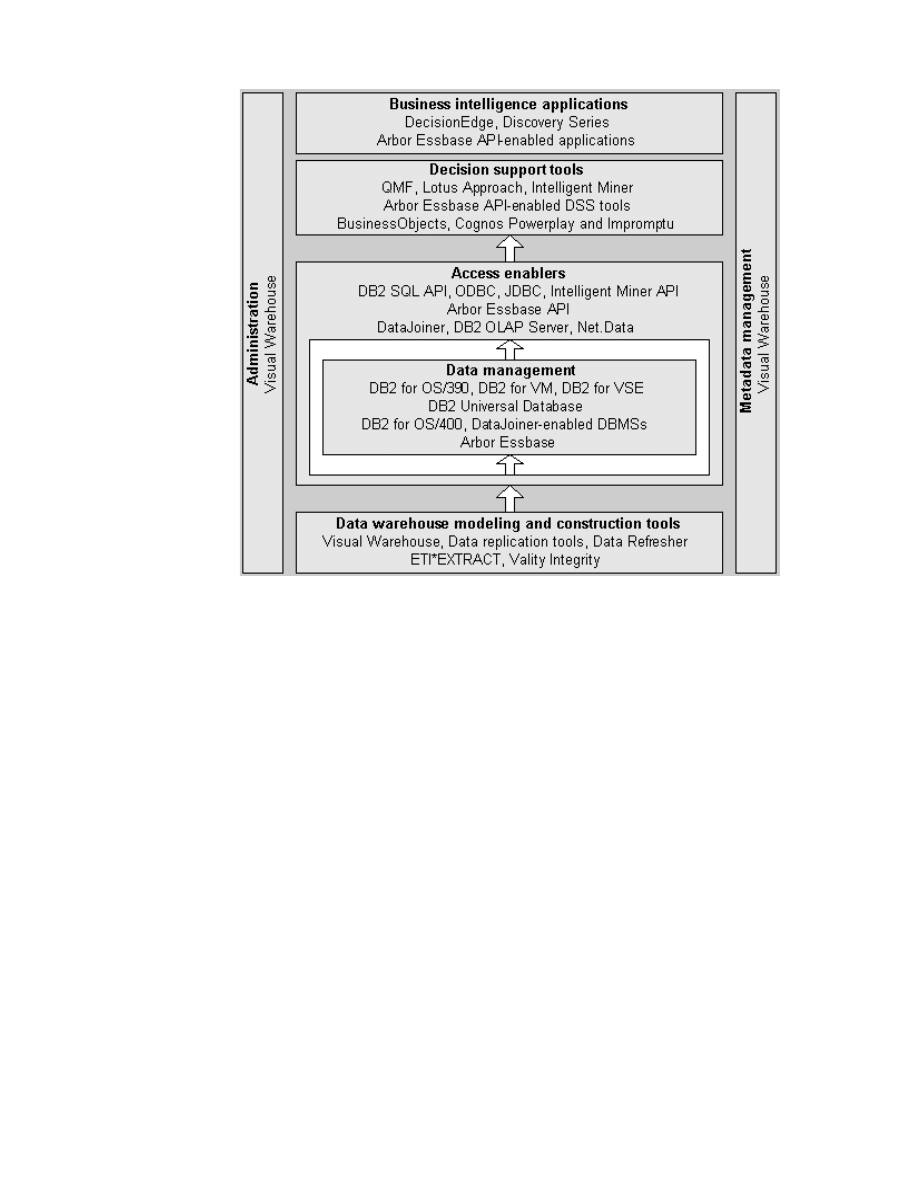
This part of the paper reviews the products and tools provided by IBM (and its
key partners) for supporting a business intelligence software environment —
these products are listed in Figure 2.
What is BI ?
9
Figure 2. IBM Business Intelligence Product Set
1.6.1 Business Intelligence Applications
IBM’s business intelligence applications are marketed under the
DecisionEdge and Discovery Series brand names. DecisionEdge is a set of
customer relationship management applications currently available for the
telecommunications and utility industries. Each DecisionEdge offering
provides integrated business applications, hardware, software, and consulting
services. DecisionEdge for Telecommunications, for example, analyzes
customer information (measuring profitability, predicting customer behavior,
analyzing attrition, and so forth) and assists in the creation of tailored
customer marketing programs. The product is used to design and deploy a
customer information data warehouse on an IBM System/390, RS/6000 or
AS/400 server using either an IBM DB2, Informix, Oracle or Sybase relational
DBMS. Business users then employ DecisionEdge packaged and customized

10
Getting Started with Data Warehouse and Business Intelligence
applications to analyze customer information, and develop and monitor
marketing programs.
Discovery Series is a set of applications and services that enable
organizations to harness the power of IBM’s Intelligent Data Miner product for
customer relationship management. Included with the Discovery Series is the
software, installation support, consulting, and training required to develop the
data models, application-specific templates, and customized graphical output
for an information mining application. The combination of services and
prebuilt applications makes it easier for organizations to see quick results
from information mining.
Business intelligence applications are also available for the DB2 OLAP
Server (see description below). This product (which was developed by IBM
and Arbor Software) employs the same API as Arbor Essbase, and can,
therefore, be used with the many industry-specific third-party application
packages available for Essbase.
1.6.2 Decision Support Tools
Business intelligence DSS tools can be broken down into three categories:
query and reporting, online analytical processing (OLAP), and information
mining.
1.6.2.1 Query and Reporting
The two main IBM query and reporting products are the Query Management
Facility (QMF) and Lotus Approach. The System/390 version of QMF has
been used for many years as a host-based query and reporting tool by DB2
for S/390 users (MVS, OS/390, VM, VSE). More recently, IBM introduced a
native Windows version of QMF. Both versions support access not only to
DB2 for S/390, but also any relational and non-relational data source
supported by its DataJoiner middleware product (see description below).
QMF host objects are compatible with QMF for Windows, extending the
enterprise query environment to Windows and the Web. Output from QMF
can be passed to other Windows applications like Lotus 1-2-3, Microsoft
Excel, Lotus Approach, and many other desktop products via Windows OLE.
Lotus Approach is a desktop relational DBMS that has gained popularity due
to its easy-to-use query and reporting capabilities. Approach can act as a
client to a DB2 family database server, and, therefore, its query and reporting
capabilities can be used to query and process DB2 data.
To increase the scope of its query and reporting offerings, IBM recently
forged relationships with Business Objects (for its BusinessObjects product)

What is BI ?
11
and Cognos (for its Impromptu and PowerPlay products). Like its key
relationships with Evolutionary Technology International, Vality Technology,
and Arbor Software, IBM intends the relationships with Business Objects and
Cognos to be more than mere joint marketing deals — they also involve
agreements to integrate the products from these companies with IBM’s
business intelligence offerings, for example, in the area of meta data
interchange.
1.6.2.2 Online Analytical Processing (OLAP)
IBM’s key product in the OLAP marketplace is the DB2 OLAP Server, which
implements a three-tier client/server architecture for performing complex
multidimensional data analysis. The middle tier of this architecture consists of
an OLAP analytical server developed in conjunction with Arbor Software,
which is responsible for handling interactive analytical processing and
automatically generating an optimal relational star schema based on the
dimensional design the user specifies. This analytical server runs on
Windows NT, OS/2, or UNIX and can be used to analyze data managed by a
DB2 Universal Database engine, or any relational database supported by
DataJoiner. The DB2 OLAP Server supports the same client API and
calculation engine as Arbor Essbase, and any of the many third-party GUI or
Web-based tools that support Essbase can act as clients to the DB2 OLAP
Server.
The value of the DB2 OLAP server lies in its ability to generate and manage
relational tables that contain multidimensional data, in the available Essbase
applications that support the product, and features within Visual Warehouse
for automating the loading of the relational star schema with information from
external data sources such as DB2, Oracle, Informix, IMS, and VSAM.
1.6.2.3 Information Mining
IBM has put significant research effort into its Intelligent Miner for Data
product, which runs on Windows NT, OS/400, UNIX and OS/390, and can
process data stored in DB2 family databases, any relational database
supported by DataJoiner, and flat files. Intelligent Miner Version 1, released in
1996, enabled users to mine structured data stored in relational databases
and flat files, and offered a wide range of different mining algorithms.
Intelligent Miner Version 2 features a new graphical interface, additional
mining algorithms, DB2 Universal Database exploitation, and improved
parallel processing.
Intelligent Miner is one of the few products on the market to support an
external API, allowing result data to be collected by other products for further
analysis (by an OLAP tool, for example). Intelligent Miner has good data

12
Getting Started with Data Warehouse and Business Intelligence
visualization capabilities, and unlike many other mining tools, supports
several information mining algorithms. IBM is also preparing to introduce its
Intelligent Miner for Text product, which will provide the ability to extract,
index, and analyze information from text sources such as documents, Web
pages, survey forms, etc.
1.6.2.4 Access Enablers
Client access to warehouse and operational data from business intelligence
tools requires a client database API. IBM and third-party business
intelligence tools support the native DB2 SQL API (provided by IBM’s Client
Application Enablers) and/or industry APIs like ODBC, X/Open CLI, and the
Arbor Essbase API.
Often, business information may be managed by more than one database
server, and IBM’s strategic product for providing access to this data is its
DataJoiner middleware server, which allows one or more clients to
transparently access data managed by multiple back-end database servers.
This federated database server capability runs on Windows NT and UNIX,
and can handle back-end servers running IBM or non-IBM data products, for
example, IBM DB2 family, Informix, Microsoft SQL Server, Oracle, Sybase,
VSAM, IMS, plus any ODBC, IBI EDA/SQL or Cross Access supported data
source. Features of this product that are worthy of note include:
• Transparent and heterogeneous database access using a single dialect of
SQL.
• Global optimization of distributed queries with query rewrite capability for
poorly coded queries.
• Stored procedure feature that allows a global DataJoiner procedure to
transparently access data or invoke a local procedure on any
DataJoiner-supported database. This feature includes support for Java
and Java Database Connectivity (JDBC).
• Heterogeneous data replication (using IBM DataPropagator, which is now
integrated with DataJoiner) between DB2, Informix, Oracle, Sybase and
Microsoft relational database products.
• Support for Web-based clients (using IBM’s Net.Data product).
IBM’s Net.Data Web server middleware tool (which is included with DB2)
supports Web access to relational and flat file data on a variety of platforms,
including the DB2 family, DataJoiner-enabled databases, and ODBC data
sources. Net.Data tightly integrates with Web server interfaces, and supports
client-side and server-side processing using applications written in Java,
REXX, Perl, C++, or its own macro language.

What is BI ?
13
1.6.2.5 Data Warehouse Modeling and Construction
IBM supports the design and construction of a data warehouse using its
Visual Warehouse product family and data replication tools, and through
third-party relationships with Evolutionary Technologies International (for its
ETI*EXTRACT Tool Suite) and Vality Technology (for its Integrity Data
Reengineering tool).
The Visual Warehouse product family is a set of integrated tools for building a
data warehouse, and includes components for defining the relationships
between the source data and warehouse information, transforming and
cleansing acquired source data, automating the warehouse load process, and
managing warehouse maintenance. Built on a DB2 core platform, Visual
Warehouse can acquire source data from any of the DB2 family of database
products, Informix, Microsoft, Oracle, Sybase, IMS databases, VSAM and flat
files, and DataJoiner-supported sources.
Organizations have the choice of two Visual Warehouse packages, both of
which are available with either Business Objects or Cognos add-ins for
information access. The base package, Visual Warehouse, includes:
• DB2 Universal Database for meta data storage.
• A Visual Warehouse Manager for defining, scheduling, and monitoring
source data acquisition and warehouse loading operations.
• A Visual Warehouse agent for performing the data capture, transformation
and load tasks.
• The Visual Warehouse Information Catalog (formerly known as
DataGuide) for exchanging meta data between administrators and
business users.
• Lotus Approach for information access.
The second package, Visual Warehouse OLAP, adds the DB2 OLAP Server
to the mix, allowing users to define and load a star schema relational
database, as well as to perform automatic precalculation and aggregation of
information as a part of the load process.
1.6.2.6 Data Management
Data management in the business intelligence environment is provided by
IBM’s DB2 family of relational DBMSs, which offers intelligent data
partitioning and parallel query and utility processing on a range of
multiprocessor hardware platforms. DB2 Universal Database on UNIX and
Windows NT additionally supports both partition and pipeline parallelism,
SQL CUBE and ROLLUP OLAP operations, integrated data replication,

14
Getting Started with Data Warehouse and Business Intelligence
dynamic bit-mapped indexing, user-defined types, and user-defined functions
(which can be written in object-oriented programming languages such as
Java).
1.7 The Challenge of Data Diversity
Rarely do medium- to large-sized organizations store all their enterprise and
departmental data in a single database management system (DBMS) or file
system. Instead, key business data is managed by multiple products
(such as DB2, Oracle, Sybase, Informix, IMS, and others) running on different
operating systems (MVS, UNIX, and Windows NT), often at widely separated
locations. For business intelligence systems, the heterogeneity of most
computing environments presents several challenges:
1. Providing users with an integrated view of the business is a key
requirement for many business intelligence systems. Therefore, business
intelligence software must be flexible enough to support diverse data
sources.
2. Similarly, a robust business intelligence solution should support
heterogeneous databases as target stores. Many companies are adopting
a multi-tiered or distributed implementations, resulting in multiple data
marts within a single company. With the increased adoption of distributed,
client/server and departmental computing, it is common for different
divisions of a company to use different database systems.
3. The foundation of an effective business intelligence solution is making it
easy for the end user to access relevant business information. A user
might need to consult the enterprise data warehouse for an answer to one
question, but for a different question, query a local data mart — or for
another, a correlation of data across a data mart and an external data
source. Making the user aware of data location adds unneeded complexity,
and discourages use of all available information.
IBM's business intelligence offerings meet the challenges of today's
heterogeneous environments. For example, IBM's DataJoiner enables easy
integration of diverse application, platform, and database environments.
Introduced in 1995 and now in its second version, DataJoiner offers features
to enable:
• Transparent heterogeneous data access: With DataJoiner, business
users need not know that they are connecting to multiple databases.
DataJoiner provides a single SQL interface that can read from and write to
diverse data sources. DataJoiner manages the complexity of establishing
connections to different data sources, translating requests into the native

What is BI ?
15
interfaces of these data sources, coping with differences in data types,
and determining an efficient data access strategy to satisfy any request.
DataJoiner allows you to treat your data marts, external data, enterprise
warehouse, and operational data store as a single, federated warehouse.
• Simpler, more powerful queries: DataJoiner makes queries in mixed and
distributed data warehouse environments simpler and more powerful than
ever. The ability to send a single query to access and join data stored in
many IBM or non-IBM, relational or non-relational, local or remote data
stores, combined with the power to employ global stored procedures,
simplifies the creation of complex business intelligence applications.
Further, DataJoiner features built-in support for Java and Java Database
Connectivity (JDBC) for Java developers.
• Optimized data access: Fast response time to queries is important to all
business users. But many of today's popular tools generate poorly
structured queries, resulting in poor performance. DataJoiner includes
sophisticated global query optimization processing, that rewrites queries
automatically — transforming poorly structured queries into an efficient,
logically equivalent form. The result? Queries perform better and are less
costly to execute. From Web browsers or classic client, DataJoiner speeds
results to demanding end users.
• Heterogeneous replication: Replication capability is vital in many data
warehouse implementations. By enabling data warehouses to be
continuously updated with changed and new operational data, business
users are given access to the latest data. And, for companies that run their
business systems 24x7, replication minimizes the reliance on batch
windows for moving data from operational systems to data warehouses.
IBM has integrated advanced replication capability into DataJoiner,
enabling heterogeneous replication between DB2, Informix, Oracle,
Sybase and Microsoft databases.

16
Getting Started with Data Warehouse and Business Intelligence

© Copyright IBM Corp. 1999
17
Chapter 2. ITSO Scenario
In this chapter we describe the network and systems setup for the IBM ITSO
San Jose center where this project was conducted. We also describe the
software and hardware that was used for the project.
2.1 The Environment
The ITSO network environment includes OS/390, VM and VSE host servers
systems, and AIX and Windows NT workstations servers. The integration of
an AS/400 system into this environment is planned for later this year.
The OS/390 and VSE systems are running as guest systems on different VM
systems located in Poughkeepsie.
On the workstation side, we used two AIX systems and three Windows NT
Server systems, one of them installed on a Netfinity server.
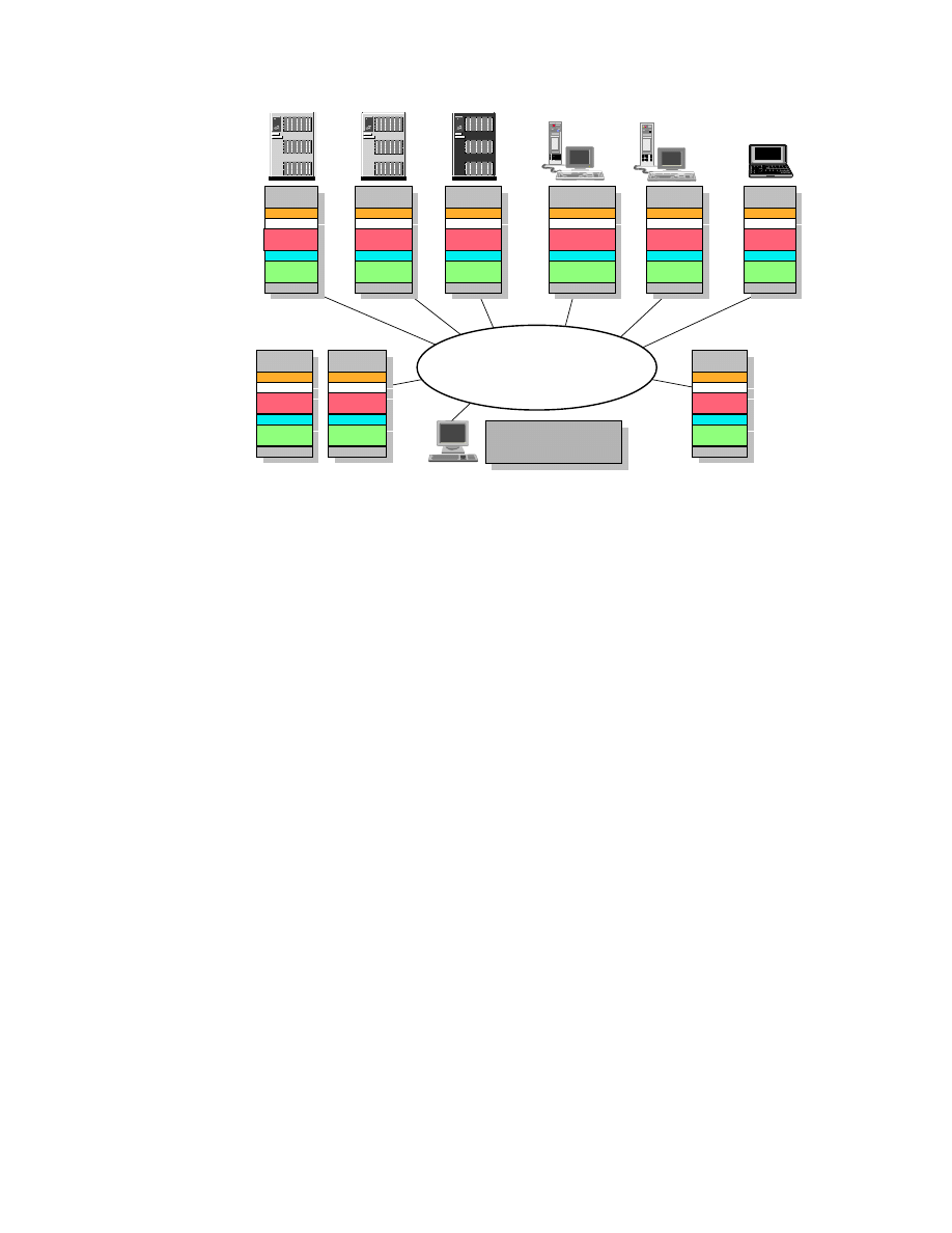
Figure 3 provides an overview of the BI environment we set up at the ITSO
center while running this project.
The systems are named by their TCP/IP hostname (workstations) or their
VTAM SSCP-name (hosts).
As you can see, this environment has all the software installed on all
platforms it is available for. Our intent was to show all the possible options for
the product installation. Therefore, we made no assumptions regarding where
to install each product for best performance, accessibility, and so on. In a real
BI environment, you will have to carefully consider which product to install on
which system, depending on the systems available for the implementation,
available products, connectivity and performance.
18
Getting Started with Data Warehouse and Business Intelligence
Figure 3. The ITSO Environment
The following sections briefly describe the installed hardware and software
according to their main functionality in the environment.
2.1.1 Database Server
The following types of relational database management systems (RDBMSs)
have been installed in the environment:
• DB2 UDB Enterprise Edition Version 5.2 on the AZOV RS/6000 system to
hold the Visual Warehouse database on AIX. The same version of DB2
UDB has been installed on the KHANKA system running under Windows
NT version 4.0.
• DB2 UDB Extended Enterprise Edition V 5.2 on the PALAU Netfinity
system to hold the Visual Warehouse database on Windows NT.
• DB2 DataJoiner Version 2.1.2 on SKY and COZUMEL for access to
non-IBM databases. These two systems also host the Classic Connect
and CrossAccess software for access to the nonrelational data sources on
the OS/390 and VSE host systems.
UDB CAE
DRDA - APPC
DRDA - TCP/IP
Classic Connect
NT, OS/2, UDB CAE, Approach,
VW Client, IM Client
Netfinity
NT
UDB EEE
ADSM
OLAP
VW Srvr.
I 586
Win95
Browser
Java
S/390
VW/VSE
DB2, DL/I,
VSAM
ADSM
AZOV
SKY
PALAU
KHANKA
COZUMEL
ITSO
Poughkeepsie
ITSO
Poughkeepsie
RS/600
AIX 4.3
VW Agnt.
ADSM
UDB EE
Oracle 8
CServ
HOD
AS/400
OS/400
DB2
ADSM
IM Data
ITSO
Rochester
SC53
SC19M (VM)
SC29M (VSE)
RS/600
AIX 4.3
VW Agnt.
DJ
DJ CC
ADSM
IM Data
I 586
NT
ADSM
WWW,CServ,
HOD, Net.Data
UDB EE
MS SQL,
CXA
VW Agnt.
DB2, IMS,
VSAM, DJCC
S/390
OS/390
ADSM
IM Data
Web Srvr.
Net.Data
I 586
NT
DJ, DJCC
CXA
ADSM
IM Data

ITSO Scenario
19
• DB2 for OS/390 Version 5 on the SC53 S/390 system at the ITSO in
Poughkeepsie. This system is the one that holds most of the operational
data.
• DB2 for VM Version 5.1 on the SC19M S/390 system at the ITSO center in
Poughkeepsie.
• DB2 for VSE Version 5.1 on the SC29M S/390 system at the ITSO center
in Poughkeepsie.
• VSAM and DL/I data sources residing on SC53 and SC29M.
• IMS data located on the SC53 system.
• DB2 for OS/400 on an AS/400 system located in Rochester.
• Oracle Version 8.0.4 on the AZOV AIX system.
• Microsoft SQL Server Version 7 on the KHANKA Windows NT system.
2.1.2 Visual Warehouse
The PALAU Netfinity server running under Windows NT Version 4.0 was
installed with the IBM Visual Warehouse Version 5.2 Server.
On all other systems that are intended to either hold the warehouse database
or that are used as communication gateways, we installed the Visual
Warehouse Agent.
2.1.3 Communication Gateways
In the current configuration of this environment, we used TCP/IP as the main
underlaying communication protocol. As the support for TCP/IP is usually
included with the operating system, there is no additional software to install.
To enhance the communication abilities of the environment, we installed the
following additional software:
• IBM Communication Server Version 5 on AIX (AZOV) and Windows NT
(KHANKA) for the APPC communication protocol support.
• IBM Host on Demand on AIX (AZOV) and Windows NT (KHANKA) for
Web-based 3270 data access.
• The World Wide Web Server has been configured on AIX (AZOV),
Windows NT (KHANKA), and S/390 (SC53). Whereas the http deamon on
AIX only has to be configured and comes with the base operating system,
we had to install a Web server software on the Windows NT server to
achieve this. We used the Lotus Domino Go Version 4.6.1 Web server.

20
Getting Started with Data Warehouse and Business Intelligence
• Net.Data Version 2.0.3 has been installed on the KHANKA Windows NT
server and the SC53 OS/390 system to provide World Wide Web access
to the databases.
2.1.4 Data Analysis Tools
To have the ability to go beyond the standard database query capability and
achieve real data exploration of the data, in the data warehouse or in the
operational data sources, we installed the following software:
• DB2 OLAP Server Version 1.0.1 has been installed on the Netfinity system
(PALAU) running under Windows NT Version 4.0 to allow Online Analytical
Processing (OLAP) of the data.
• IBM Intelligent Miner for Data Version 2.1.3 Server for data mining
capability has been installed on AIX (SKY), Windows NT (COZUMEL),
OS/390 (SC53), and OS/400. The Intelligent Miner for Data client code
has been installed on AIX (AZOV) and Windows NT (COZUMEL).
2.2 The Data
One major part of this scenario consists of the data and the data sources. We
have been provided with quite a large database, and its data has been stored
on the OS/390 system into DB2, VSAM, and IMS databases; and on the VSE
system into DB2, VSAM, and DL/I database.
To give you an idea of the amount of data, here some figures:
The largest DB2 table has a rowcount of more than 3,500,000 with an
average rowlength of about 80 bytes. All DB2 tables together occupy about
700 MB of disk space.
The VSAM KSDS cluster has more than 740,000 636-byte records, which is
more than 450 MB of data. Due to the VSAM specifications, there are no
more than 2 records in one 2048-byte control interval. So the file occupies
more than 727 MB of disk space.
The following is a description of the data provided. As mentioned above, we
have three different kinds of data sources: DB2, DL/I and VSAM. But all data
ends up in DB2 tables on the workstation side. Even the VSAM and DL/I data
is already referenced on the host side as relational tables through
CrossAccess. Therefore, the data description does not follow the data
sources, but rather the usage of the data.

ITSO Scenario
21
2.2.1 Sales Information
The sales information is contained in one DB2 table called SALE_DAY_003,
which holds data from the stores scanner cashiers. The ’003’ in the name
identifies this data being captured for the company stores belonging to the
product segment group ’3’ (’PRODNO = 3.’ in the other tables), which means
that only data belonging to that product segment group is to be populated to
the data warehouse.
This table contains sales information, such as:
• Basic article number
• Product grouping number
• Supplier identification
• Sales per store and article on a daily basis
• Date, the article was sold
• Number of sold units
• Retail price including tax
• Sales tax
2.2.2 Article Information
The article information tables have all the data about the articles, their
structuring, relation to suppliers and supplier data. These tables are mostly
from DB2 except the supplier data, which is derived from VSAM. The main
table content and table names are listed below.
The table called BASART holds basic article information, such as:
• Basic article number
• Article description
• Creation date of the database entry
• Color
The table called ARTTXT contains more data on the article description,
such as:
• Basic article number
• Product segment grouping
• Company number
• Store number

22
Getting Started with Data Warehouse and Business Intelligence
The table called STRUCTART holds article structuring information, such as:
• Basic article number
• Product segment grouping
• Price range number
The table called STRARTDAT contains additional article structuring
information, such as:
• Basic article number
• Product segment grouping
• Store number
• Date until the article is valid
• Date since the article is available
• Units for retail
• Product group
The table called WGRARTST003 contains article grouping data for
PRODNO=3, such as:
• Company number
• Product group number
• Product group description
• Creation date of entry
• Changing date of entry
The table called DEPOT holds the information about the relationship to the
product line, brand, and supplier, such as:
• Product segment grouping
• Company number
• Price range number
• Depot number
• Depot description
• Creation date of entry

ITSO Scenario
23
The table called SUPPLART contains information about the relationship to
the suppliers and order information, such as:
• Base article number
• Supplier number
• Price range number
• Store number
• Creation date of entry
• Deletion marker
• Account to be billed
• Delivery unit
• Supply unit
• Delivery time
The table called SUPPLIER holds detailed information about the suppliers,
such as:
• Supplier number
• Supplier name
• Company number
• Supplier address
2.2.3 Organization Information
The organization information consists of data from all data sources. The
information about the business lines is taken from a new DB2 table, the
company data is derived from the DL/I database, and the information about
the stores comes from the VSAM data set. The organization structure table
(ORGA_STRUC) from DB2 is not used in this project, because the available
sales data relates to one product segment group (3) only. The following
describes the tables and their organization.
The ORGSTRUCT table holds data such as:
• Product segment grouping
• Company number
• Price range number
• Store number

24
Getting Started with Data Warehouse and Business Intelligence
The table called STORES is derived from the VTAM data set, and describes
the different stores with information, such as:
• Company number
• Store number
• Store address
• Sales space in square meter
• Sales manager ID
• Date store was opened
The COMPANY_DB is taken from DL/I and contains information, such as:
• Company number
• Company name
• Business line
• Company group ID
2.3 Data Warehouse for OLAP
To build up the data warehouse for OLAP with three different dimensions
(article, organization, and time) a large amount of this data has to be
replicated to the workstation databases.
Here we provide a little description of the databases and tables we used.
Because the data warehousing and OLAP are based on relational data
sources, we had to transform the DL/I (IMS) and VSAM data into DB2 tables.
We describe only the tables and columns used to build the data warehouse
sources for OLAP, starting with the DB2 tables contained in the VSE
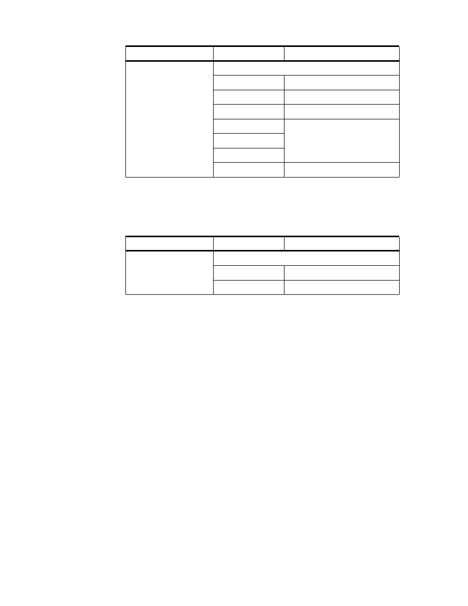
database as shown in Table 1.
Table 1. DB2 Tables on SC19M
Table Name
Column Name
Description
STRUC_ARTICLE
Structure of articles
BASARTNO
Basic article number
DEL_MARK
delete marker
DELETE_DATE
date entry was marked ’deleted’
PRODNO
product segment number (= 3.0)

ITSO Scenario
25
SUPPLIERS_ARTICLE
Article to supplier relation
BASARTNO
basic article number
SUPPLNO
supplier number
DEPOTNO
product line number
PRODNO
product segment number (= 3.0)
DEL_MARK
delete marker (^= ’L’ to avoid
duplicate article numbers)
ARTICLE_TXT
Article description
BASARTNO
basic article number
ARTICLE_TEXT
article description
TXTTYPNO
type of ARTICLE_TEXT
( 1.0 = name / 2.0 = content )
PRODNO
product segment number (= 3.0)
DEPOT
Depot (brand) and product line description
BASARTNO
basic article number
TEXT_DEPOT
product brand (supplier)
description
TEXT_LINE
product line description
SUPPLNO
supplier number
DEPOTNO
DEPTNO (6:7) = 00 --> brand ID
DEPTNO (6:7) > 00 --> line ID
PRODNO
product segment number (= 3.0)
Table Name
Column Name
Description

26
Getting Started with Data Warehouse and Business Intelligence
* STORENO is only unique together with COMPNO!
The data about the organization and the suppliers is derived from the DL/I
and VSAM data. By using CrossAccess and the appropriate meta data
definitions, we created Table 2 and Table 3:
Table 2. DL/I ’Tables’ derived through CrossAccess
SALE_DAY_003
Sold articles per day and per store
BASARTNO
Basic article number
STORENO
Store number *
COMPNO
Company number *
NO_UNITS
Number of sold units
IN_PRC
Price for buying the article (DM)
OUT_PRC
Price the article was sold for
multiplied by NO_UNITS (DM)
TAX
Amount of tax (DM)
NO_CUST
Number of customers
Table Name
Column Name
Description
COMPANY_DB
Base of companies belonging to the organization
COMPNO
Company number
NAME
Company name
B_LINE
Business line for this company
Table Name
Column Name
Description
ITSO Scenario
27
Table 3. VSAM ’Tables’ derived through CrossAccess
For the organization information, we needed an additional data source
providing the data for the business lines. So we generated an additional
database ’SJNTADD’ on the Windows NT Server workstation ’KHANKA’. See
Table 4 below.
Table 4. DB2 Table in Windows NT database SJNTADD
Table Name
Column Name
Description
STORES
Base of stores belonging to the companies
STORENO
Store number
NAME
Store name
COMPNO
Company number
STREET
Address of store
ZIP
CITY
REGION_MGR
Region (manager) ID
Table Name
Column Name
Description
BUSINESS_LINES
business line definitions
BL_NO
business line ID
BL_NAME
business line name

28
Getting Started with Data Warehouse and Business Intelligence

© Copyright IBM Corp. 1999
29
Chapter 3. The Products and Their Construction
In this chapter we describe briefly the products that were used for the IBM
ITSO project. Detailed information about each product can be found in their
own manuals.
3.1 The DataJoiner Product
DataJoiner is a multidatabase server that provides access to data in multiple
heterogeneous sources, including IBM and non-IBM, relational and
nonrelational, and local and remote sources. DataJoiner includes integrated
replication administration, support for Java applications, query optimization
technology, industry-standard SQL (across all data source types), and both
synchronous and asynchronous data access. DataJoiner allows you to
access all data in your enterprise as if it were local. It is currently available for
Windows NT and UNIX.
DataJoiner provides all the major functional enhancements provided by DB2.
Also, Datajoiner supports geographic information system (GIS) data.
3.1.1 DataJoiner Classic Connect Component
DataJoiner Classic Connect is a separately-orderable component of
DataJoiner that provides access to nonrelational data stored in Information
Management Systems (IMS) databases and Virtual Storage Access Method
(VSAM) data sets on OS/390. It provides communication, data access, and
data mapping functions so you can access nonrelational data using relational
queries.
DataJoiner Classic Connect requires the DataJoiner software product in order
to allow you to connect to DataJoiner databases, and DataJoiner instances. A
solution with DataJoiner Classic Connect and a DataJoiner instance together,
allows users from several different platforms to submit an SQL query that
accesses nonrelational data.
DataJoiner Classic Connect provides read-only relational access to IMS
databases and VSAM data sets. It creates a logical, relational database,
complete with logical tables that are mapped to actual data in IMS or VSAM
databases. Using this relational structure, Classic Connect interprets
relational queries that are submitted by users against IMS and VSAM data
sets.

30
Getting Started with Data Warehouse and Business Intelligence
3.1.2 DataJoiner Classic Connect Architecture
Figure 4 on page 33 shows the Classic Connect architecture, which consists
of the following major components:
• Client Interface Module:
The client interface module is used to establish and maintain connections
with data servers and Enterprise Servers. It performs the following
functions:
• Determines and loads the appopiate transport layer module, based on
configuration parameters
• Establishes communications with data servers and Enterprise Servers
• De-references host variables in SQL statements
• Stores and retrieves data in the application storage areas
• Presents error and feedback information to the application
The client interface module can establish multiple connections to a data
server or Enterprise Server on behalf of a single application program.
• Classic Connect Data Server:
Classic Connect data server is responsible for all data access. It performs
the following functions:
• Accepting SQL queries from DataJoiner or the sample applications
(DJXSAMP).
• Determining the type of data to be accessed.
• Rewriting the SQL query into the native file or database access
language needed. A single SQL access could translate into multiple
native requests.
• Optimizing queries based on generic SQL query rewrite and file — or
database-specific optimization.
• Querying multiple data sources for JOINs.
• Translating result sets into a consistent relational format, which
involves restructuring non-relational data into columns and rows.
• Sorting result sets as needed; such as ORDER BY.
• Issuing all client catalog queries to the Classic Connect meta data
catalog.
The following components run in the data server:
• Region Controller Services — This data server component is
responsible for starting, stopping, and monitoring all of the other

The Products and Their Construction
31
components of the data server. It determines which services to start
based on SERVICE INFO ENTRY parameters at the Data Server
Master configuration file on OS/390.
• Initialization Services — This data server component is responsible for
initializing and terminating different types of interfaces to underlying
database management systems or MVS systems components such as
IMS BMP/DBB initialization service, IMS DRA initialization service, and
WLM initialization service.
• Connection Handler Services — This data server component is
responsible for listening for connection requests from DataJoiner.
Connection requests are routed to the appropriate query processor
task for subsequent processing.
• Query Processor Services — This data server component is
responsible for translating client SQL into database and file-specific
data access requests.
• Logger Services — This data serve component is used for system
monitoring and trouble shooting. A single logger task can be running
within a data server. During normal operations, you will not need to be
concerned with the logger service.
• Enterprise Server:
The Enterprise Server is an optional component that you can use to
manage a large number of concurrent users across multiple data sources
(see Figure 5 on page 34). Like a data server, the Enterprise Server’s
connection handler is responsible for listening for client connection
requests. However, when a connection request is received, the Enterprise
Server does not forward the request to a query processor task for
processing. Instead, the connection request is forwarded to a data source
handler (DSH) and then to a data server for processing. The Enterprise
Server maintains the end-to-end connection between the client application
and the target data server. It is responsible for sending and receiving
messages between the client application and the data server.
The Enterprise Server determines the locations of the data servers that it
will be communicating with through the configuration parameters. Also, it
determines whether those data servers are running on the platform as the
Enterprise Server.
The Enterprise Server can automatically start a local data server if there
are no instances active. It can also start additional instances of a local
data server when the currently active instances have reached the
maximum number of concurrent users they can service, or the currently
active instances are all busy.

32
Getting Started with Data Warehouse and Business Intelligence
• Data Mapper:
The Classic Connect nonrelational data mapper is a Microsoft
Windows-based application that automates many of the tasks required to
create logical table definitions for nonrelational data structures. The data
mapper interprets existing physical data definitions that define both the
content and the structure of nonrelational data.
The data mapper accomplishes the creation of logical table definitions for
nonrelational data structures, by creating meta data grammar from
existing nonrelational data definitions. The meta data grammar is used as
input to the Classic Connect meta data utility to create a meta data catalog
that defines how the nonrelational data structure is mapped to an
equivalent logical table. The meta data catalogs are used by query
processor tasks to facilitate both the access and translation of the data
from the nonrelational data structure into relational result sets.
The data mapper import utilities create initial logical tables from COBOL
copybooks. A visual point-and-click environment is used to refine these
initial logical tables to match site- and user-specific requirements. You can
utilize the initial table definitions automatically created by data mapper, or
customize those definitions as needed.
It is possible to create multiple logical tables that map to a single physical
file or database. With this facility you can customize these table definitions
to the needs of the user. The data mapper contains embedded FTP
support of facilitate file transfer from and to the mainframe.
Figure 6 on page 35 shows the Data Mapper workflow.
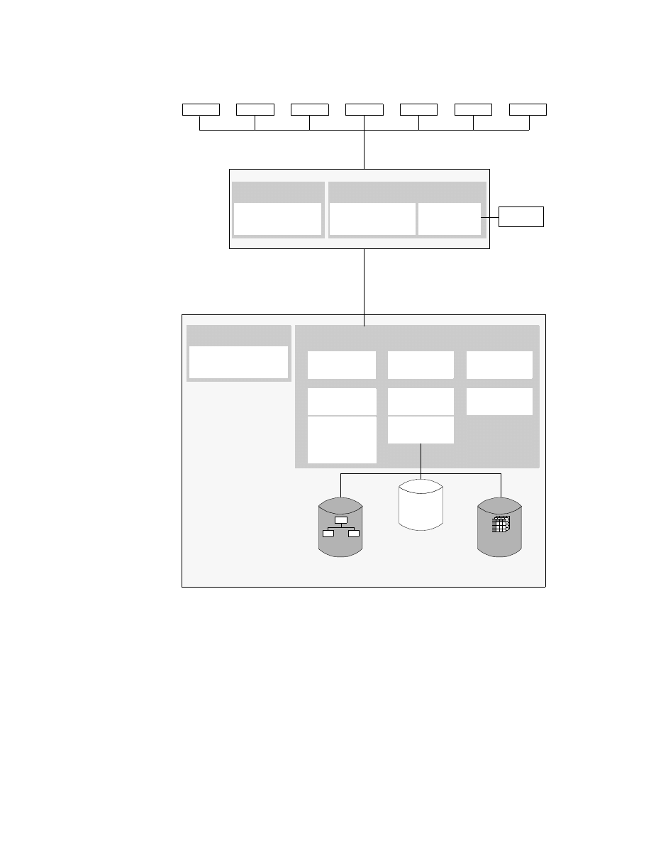
The Products and Their Construction
33
Figure 4. Classic Connect Architecture
MVS Sample Application
(DJXSAMP) with
client interface module
Region Controller
Tasks
Classic Connect
Data Server
MVS
Operator
Logger tasks
Connection
Handler
Multiple Query
Processor
System
Exit
Transport layer
• TCP/IP
• SNA LU6.2
• Cross Memory
OS/2
AIX
DOS
Windows
HP-UX
Solaris
Others
Client Platforms Using DB2
Sample Application
(DJXSAMP2) with
client interface module
Classic Connect data
access module with
client interface module
DataJoiner Instance
AIX/NT
IMS
DATA
VSAM
DATA
Other data
access module
Other
data
sources
SSIs
Meta Data
Catalogs
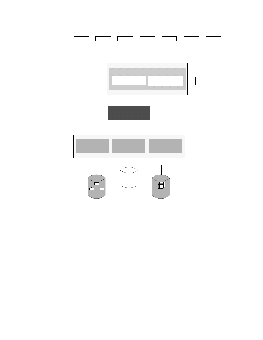
34
Getting Started with Data Warehouse and Business Intelligence
Figure 5. Classic Connect Architecture with Enterprise Server
MVS
OS/2
AIX
DOS
Windows
HP-UX
Solaris
Others
Client Platform Application
DataJoiner Instance
AIX
IMS
DATA
VSAM
DATA
Other data
access module
Other data
sources
MVS
Classic Connect data
access module
Classic Connect
Enterprise Server
Classic Connect
Data Server
Meta Data
Catalogs
Classic Connect
Data Server
Classic Connect
Data Server

The Products and Their Construction
35
Figure 6. Data Mapper Workflow
PC
SERVER
File Definition
Source
Step 3:
Generate Meta data grammar
Step 2: Customize
Target Database
Definition
File Definition
Source
Meta Data
Catalogs
*
Meta Data
Utility
Step 1: Import data descriptions
DBDs or COBOL
copybooks
Meta Data
Grammar
DataMapper
Step 4:
Export Meta
Data
*
SYSIBM.SYSTABLES
SYSIBM.SYSCOLUMNS
SYSIBM.SYSINDEXES
SYSIBM.SYSKEYS
SYSIBM.SYSTABAUTH

36
Getting Started with Data Warehouse and Business Intelligence
3.2 CrossAccess
CrossAccess from CROSS ACCESS Corporation (
www.crossaccess.com
)
provides relational access to nonrelational data stored in VSAM, DL/I,
sequential, ADABAS, Datacom and IDMS. It provides communication, data
access, and data mapping functions so you can access nonrelational data
using relational queries.
3.2.1 CrossAccess Architecture
Figure 7 on page 39 shows the CrossAccess architecture, which consists of
the following major components:
• CrossAccess Data Server:
CrossAccess data server is responsible for all data access. It performs the
following functions:
• Accepting SQL queries from ODBC clients or the sample applications
(CXASAMP).
• Determining the type of data to be accessed.
• Rewriting the SQL query into the native file or database access
language needed. A single SQL access could translate into multiple
native requests.
• Optimizing queries based on generic SQL query rewrite and file—or
database-specific optimization.
• Querying multiple data sources for JOINs.
• Translating result sets into a consistent relational format, which
involves restructuring non-relational data into columns and rows.
• Sorting result sets as needed; such as ORDER BY.
• Issuing all client catalog queries to the CrossAccess meta data catalog.
• Stored procedure interface, which allows an Assembler, COBOL, or PLI
application program to be invoked.
The following components run on the data server:
Region Controller Services—This data server component is responsible
for starting, stopping, and monitoring all of the other components of the
data server. It determines which services to start based on SERVICE
INFO ENTRY parameters in the Data Server Master configuration file.
Initialization Services—This data server component is responsible for
initializing and terminating different types of interfaces to underlying

The Products and Their Construction
37
database management systems or systems components such as
Language Environment (LE) or WLM initialization service.
Connection Handler Services—This data server component is responsible
for listening for connection requests from ODBC clients. Connection
requests are routed to the appropriate query processor task for
subsequent processing.
Query Processor Services—This data server component is responsible for
translating client SQL into database and file-specific data access
requests.
Logger Services—This data serve component is used for system
monitoring and trouble shooting. A single logger task can be running
within a data server. During normal operations, you will not be concerned
with the logger service.
• Enterprise Server:
The Enterprise Server is an optional component that you can use to
manage a large number of concurrent users across multiple data sources
(see Figure 8 on page 40). Like a data server, the Enterprise Server’s
connection handler is responsible for listening for client connection
requests. However, when a connection request is received, the Enterprise
Server does not forward the request to a query processor task for
processing. Instead, the connection request is forwarded to a data source
handler (DSH) and then to a Data Server for processing. The Enterprise
Server maintains the end-to-end connection between the client application
and the target data server. It is responsible for sending and receiving
messages between the client application and the data server.
The Enterprise Server determines the locations of the data servers that it
will be communicating with through the configuration parameters. Also, it
determines whether those data servers are running on the same platform
as the Enterprise Server.
The Enterprise Server can automatically start a local Data Server if there
are no instances active. It can also start additional instances of a local
data server when the currently active instances have reached the
maximum number of concurrent users they can service, or the currently
active instances are all busy.
• Data Mapper:
The CrossAccess nonrelational Data Mapper is a Microsoft
Windows-based application that automates many of the tasks required to
create logical table definitions for nonrelational data structures. The Data

38
Getting Started with Data Warehouse and Business Intelligence
Mapper interprets existing physical data definitions that define both the
content and the structure of nonrelational data.
The Data Mapper accomplishes the creation of logical table definitions for
nonrelational data structures by creating meta data grammar from existing
nonrelational data definitions. The meta data grammar is used as input to
the CrossAccess meta data utility to create a meta data catalog that
defines how the nonrelational data structure is mapped to an equivalent
logical table. The meta data catalogs are used by query processor tasks to
facilitate both the access and translation of the data from the nonrelational
data structure into relational result sets.
The Data Mapper import utilities create initial logical tables from COBOL
copybooks. A visual point-and-click environment is used to refine these
initial logical tables to match site- and user-specific requirements. You can
utilize the initial table definitions automatically created by Data Mapper, or
customize those definitions as needed.
It is possible to create multiple logical tables that map to a single physical
file or database. With this facility you can customize these table definitions
to the needs of the user. Figure 9 on page 41 shows the Data Mapper
workflow.
• Client Interface Module:
The client interface module is used to establish and maintain connections
with Data Servers and Enterprise Servers. It performs the following
functions:
• Determines and loads the appropriate transport layer module, based
on configuration parameters
• Establishes communications with Data Servers and Enterprise Servers
• De-references host variables in SQL statements
• Stores and retrieves data in the application storage areas
• Presents error and feedback information to the application
The Client Interface Module can establish multiple connections to a Data
Server or Enterprise server on behalf of a single application program.
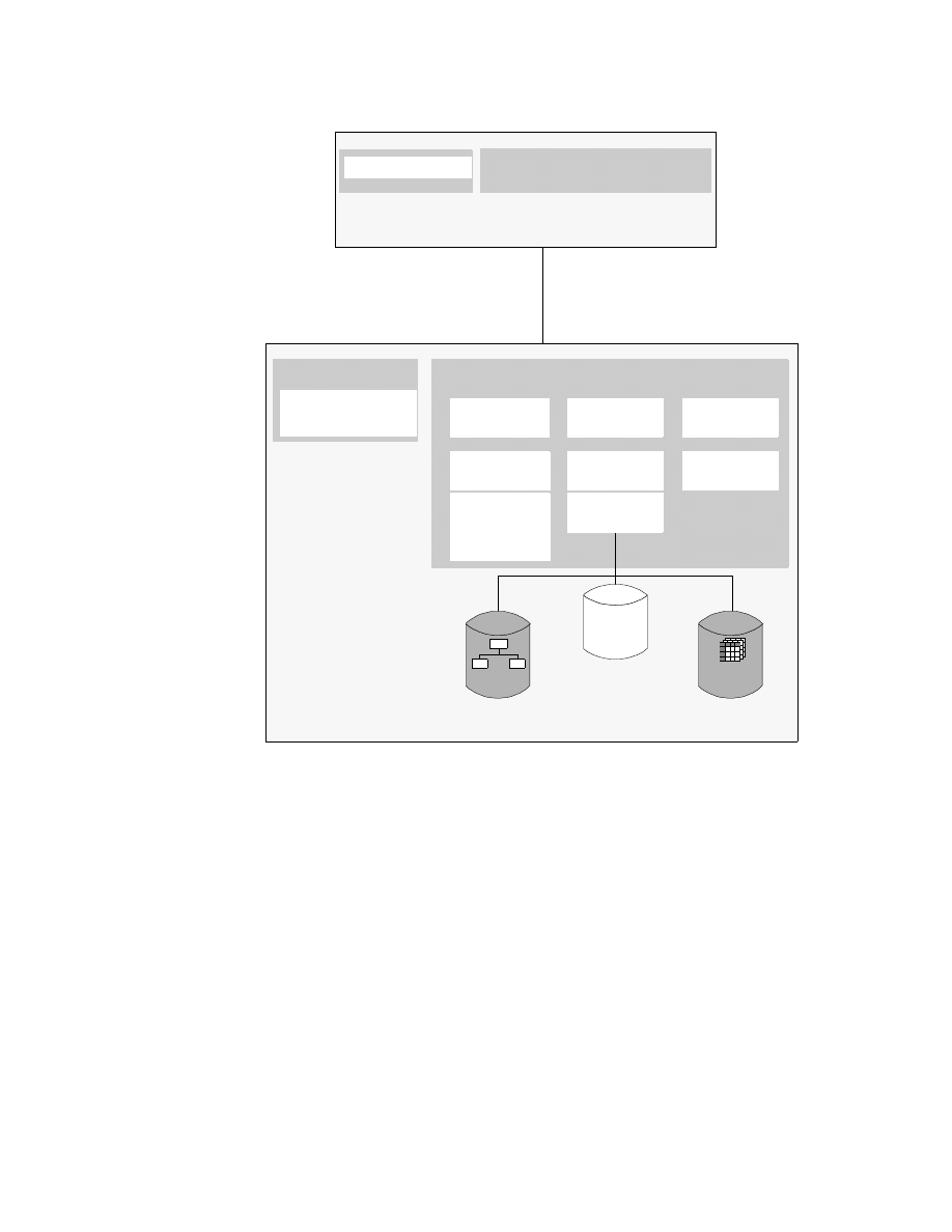
The Products and Their Construction
39
Figure 7. CrossAccess Architecture
Sample Application
(CXASAMP) with
client interface module
Region Controller
Tasks
CrossAccess
Data Server
MVS or VSE
Operator
Logger tasks
Connection
Handler
Multiple Query
Processor
System
Exits
Transport layer
• TCP/IP
• SNA LU6.2
• Cross Memory
ODBC Application
CrossAccess ODBC Client
Windows Workstation
DL/I
DATA
VSAM
DATA
SSIs
Meta Data
Catalogs
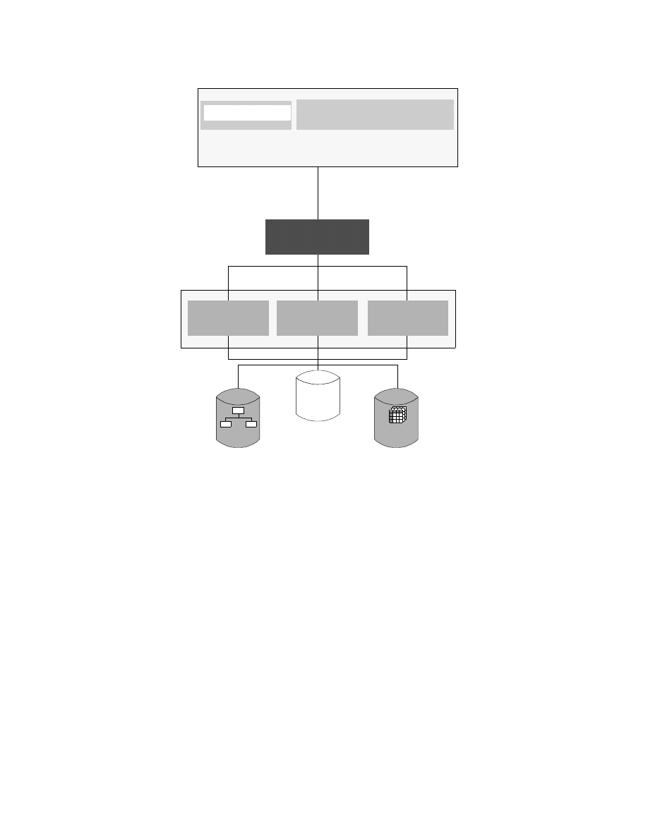
40
Getting Started with Data Warehouse and Business Intelligence
Figure 8. CrossAccess Architecture with Enterprise Server
MVS
or VSE
DL/I
DATA
VSAM
DATA
MVS or VSE
CrossAccess
Enterprise Server
CrossAccess
Data Server
Meta Data
Catalogs
CrossAccess
Data Server
CrossAccess
Data Server
ODBC Application
CrossAccess ODBC Client
Windows Workstation
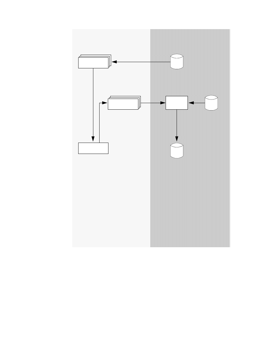
The Products and Their Construction
41
Figure 9. CrossAccess Data Mapper Workflow
PC
SERVER
File Definition
Source
Step 3:
Generate Meta data grammar
Step 2: Customize
Target Database
Definition
File Definition
Source
Meta Data
Catalogs
*
Meta Data
Utility
Step 1: Import data descriptions
DBDs or COBOL
copybooks
Meta Data
Grammar
DataMapper
Step 4:
Export Meta
Data
*
SYSIBM.SYSTABLES
SYSIBM.SYSCOLUMNS
SYSIBM.SYSINDEXES
SYSIBM.SYSKEYS
SYSIBM.SYSTABAUTH

42
Getting Started with Data Warehouse and Business Intelligence
The Data Mapper contains embedded FTP support to facilitate file transfer
from and to the mainframe.
3.3 Visual Warehouse: Server and Agent
Visual Warehouse is an integrated product for building and maintaining a data
warehouse or data mart in a LAN environment. Visual Warehouse does not
simply create a data warehouse or an informational database; it provides the
processes to define, build, manage, monitor, and maintain an informational
environment. It integrates many of the business intelligence component
functions into a single product. It can be used to automate the process of
bringing data together from heterogeneous sources into a central, integrated,
informational environment.
Visual Warehouse can be managed either centrally or from the workgroup
environment. Therefore, business groups can meet and manage their own
information needs without burdening information systems resources, thus
enjoying the autonomy of their own data mart without compromising overall
data integrity and security in the enterprise.
3.3.1 Data Sources Supported
Visual Warehouse provides the capability to extract and transform data from
a wide range of heterogeneous data sources, either internal or external to the
enterprise, such as the DB2 family, Oracle, Sybase, Informix, Microsoft SQL
Server, VSAM, IMS, and flat files (for example, from spreadsheets). Data
from these sources is extracted and transformed based on meta data defined
by the administrative component of Visual Warehouse. The extract process,
which supports full refreshes of data, can run on demand or on an automated
scheduled basis.
3.3.2 Data Stores Supported
The transformed data can be placed in a data warehouse built on any of the
DB2 UDB platforms, including DB2 for Windows NT, DB2 for AIX, DB2 for
HP-UX, DB2 for Sun Solaris, DB2 for SCO, DB2 for SINIX, DB2 for OS/2,
DB2 for OS/400, and DB2 for OS/390, or on flat files. Visual Warehouse
provides the flexibility and scalability to populate any combination of the
supported databases.
Visual Warehouse also supports Oracle, Sybase, Informix, and Microsoft SQL
Server using IBM DataJoiner.

The Products and Their Construction
43
3.3.3 End User Query Tools
Once the data is in the target data warehouse, it is accessible by a variety of
end user query tools. Those tools can be from IBM, such as Lotus Approach,
or QMF for Windows, or from any other vendors whose products comply with
the DB2 Client Application Enabler (CAE) or the Open Database Connectivity
(ODBC) interface, such as Business Objects, Cognos Impromptu, and Brio
Query. The data can also be accessed using a popular Web browser with
additional Web infrastructure components.
3.3.4 Meta Data Management
Visual Warehouse stores all the meta data in its control database and is
integrated with DataGuide, IBM’s meta data management tool, which is part
of the Visual Warehouse solution. The data warehouse model, which defines
the structure and contents of the data warehouse, is stored in the meta data
repository. For each data source to be accessed, Visual Warehouse first
extracts the meta data that describes the contents of the data source and
places it in the meta data repository. This meta data is then used to extract,
filter, transform, and map the source data to the data warehouse.
The meta data of Visual Warehouse can then be transferred to the
Information Catalog managed by DataGuide. With DataGuide, users can
create an Information Catalog, which contains graphical representations of
the meta data. DataGuide can be integrated with DB2 CAE entitled decision
support tools, which can be used to view the meta data specific to an object
of interest in the DataGuide Information Catalog.
3.3.5 The Architecture of Visual Warehouse
The Visual Warehouse architecture provides a fully distributed Client/Server
system that lets users reap the benefits of network computing. The
architecture consists of the following major components:
• Server
• Administrative Clients
• Agents
• Control Database
• Target Databases
3.3.5.1 Visual Warehouse Server
Visual Warehouse Server, which runs on a Windows NT workstation or
server, controls the interaction of the various data warehouse components
and provides for automation of data warehousing processes by a powerful

44
Getting Started with Data Warehouse and Business Intelligence
scheduling facility, which allows calendar-based scheduling as well as
event-based scheduling. The server component monitors and manages the
data warehousing processes. It also controls the activities performed by the
Visual Warehouse agents.
3.3.5.2 Visual Warehouse Administrative Clients
The Administrative Client, which also runs on a Windows NT workstation or
server, provides an interface for administrative functions, such as defining the
business views, registering data resources, filtering source data, defining the
target data warehouse databases, managing security, determining the data
refresh schedules, and monitoring the execution of the data warehouse
processes. Visual Warehouse can support an unlimited number of
administrative clients and provides comprehensive security facilities to
control and manage client access to the administrative functions.
3.3.5.3 Visual Warehouse Agents
Visual Warehouse agents handle access to the source data, filtering,
transformation, subsetting, and delivery of transformed data to the target
warehouse under the direction of the Visual Warehouse Server.
Visual Warehouse agents run on Windows NT, OS/2, AS/400, AIX, and Sun
Solaris. Visual Warehouse supports an unlimited number of agents. Because
multiple agents can participate in the population of a data warehouse, the
throughput can significantly increase when multiple agents act
simultaneously. The agents primarily use ODBC drivers as the means of
communicating with different data sources and targets.
The Visual Warehouse agents architecture is a key enabler for scalable
business intelligence solutions.
3.3.5.4 Visual Warehouse Control Database
A control database must be set up in DB2 to be used by Visual Warehouse to
store control information used by the Visual Warehouse Server. The control
database stores all the meta data necessary to build and manage the
warehouse. The information in the control database includes the mappings
between the source and target data, the schedules for data refresh, the
Business Views, and operational logs. The control database is managed by
the Visual Warehouse Administrator and used by the Visual Warehouse
agents. When a request for service is made to the Visual Warehouse Server,
the control information pertinent to that request is retrieved from the control
database and sent to the appropriate agent that actually provides the service.
Note that different warehouses could use different control databases.

The Products and Their Construction
45
Advanced DB2 features, such as triggers and stored procedures, can be
used in conjunction with the Visual Warehouse control data to provide an
advanced operating environment. For instance, DB2 triggers can be used to
monitor log inserts and to send out alert signals through DB2 stored
procedures when a certain event occurs.
3.3.5.5 Visual Warehouse Target Databases
Target databases in a data warehouse contain the Visual Warehouse data
stored in structures defined as Business Views (BVs). When Visual
Warehouse populates a BV, data is extracted from the source, transformed
according to the rules defined in the BV, and then stored in the target
database. Multiple databases could be used as target databases for a data
warehouse.
3.4 Intelligent Miner for Data
Data mining can be defined as the process of automatically extracting valid,
useful, previously unknown, and ultimately comprehensible information from
large databases and using it to make crucial business decisions.
The Intelligent Miner (IM) helps us perform data mining tasks. Through an
intuitive graphical user interface (GUI) you can visually design data mining
operations. You can choose tools and customize them to meet your
requirements. The available tools cover the whole spectrum of data mining
functions. In addition IM selects data, explores it, transforms it, and visually
interprets the results for productive and efficient knowledge discovery.
3.4.1 Overview of the Intelligent Miner
The IM is based on a client-server architecture. The server executes mining
and processing functions and can host historical data and mining results. The
client is powered with administrative and visualization tools and can be used
to visually build a data mining operation, execute it on the server, and have
the results returned for visualization and further analysis. In addition, the IM
application programing interface (API) provides C++ classes and methods as
well as C structures and functions for application programers.
3.4.2 Working with Databases
Most functions of the IM can use input data from either flat files or database
tables. If you want to access DB2 tables, you only require authorization to
access that database and the permission to query the appropriate tables. If
you want to access files in Oracle, SPSS, or SAS format, DataJoiner may be
installed as a middleware product.

46
Getting Started with Data Warehouse and Business Intelligence
There are two ways to access database management systems:
• Connect through the Intelligent Miner server without installing any
database software in the client.
• Connect directly from the client to the table, letting the IM client access the
database without using the IM communication interface.
3.4.3 The User Interface
The IM helps businesses reduce the cost of data mining and maximize the
return on investment (ROI), providing an administrative user interface based
on Java. The IM user interface is simple and intuitive and provides
consistency across all operations. The interface’s state-of-the-art GUI
facilities include online help, task guides, and a graphical representation of
the mining operations and its functions.
3.4.4 Data Preparation Functions
Once the desired database tables have been selected and the data to be
mined has been identified, it is usually necessary to perform certain
transformations on the data. IM provides a wide range of data preparation
functions which help to optimize the performance of the data mining
functions. Depending on the data mining technique, you can select, sample,
aggregate, filter, cleanse, and/or transform data in preparation for mining.
The data preparation functions are:
• Aggregate values
• Calculate values
• Clean up data sources
• Convert to lower or upper case
• Copy records to file
• Discard records with missing values
• Discretize into quantiles
• Discretize using ranges
• Encode missing values
• Encode nonvalid values
• Filter fields
• Filter records
• Filter records using a value set

The Products and Their Construction
47
• Get random sample
• Group records
• Join data sources
• Map values
• Pivot fields to records
• Run SQL statements
Data preparation functions are performed through the GUI, reducing the time
and complexity of data mining operations. You can transform variables,
impute missing values, and create new fields through the touch of a button.
This automation of the most typical data preparation tasks is aimed at
improving your productivity by eliminating the need for programming
specialized routines.
3.4.5 Statistical and Mining Functions
After transforming the data we use one or more data mining functions in order
to extract the desired type of information. IM provides both statistical analysis
tools and state of the art machine learning algorithms for successful data
mining.
Statistical functions facilitate the analysis and preparation of data, as well as
providing forecasting capabilities. For example, you can apply statistical
functions like regression to understand hidden relationships in the data or use
factor analysis to reduce the number of input variables. Statistical functions
include:
• Factor analysis
• Linear regression
• Principal component analysis
• Univariate curve fitting
• Univariate and bivariate statistics
Based on IBM research, validated through real-world applications, IM has
incorporated a number of data mining algorithms as the critical suite to
address a wide range of business problems. The algorithms are categorized
as follows:
• Association discovery:
Given a collection of items and a set of records, each of which contains
some number of items from the given collection, an association discovery

48
Getting Started with Data Warehouse and Business Intelligence
function is an operation against this set of records which returns affinities
that exist.
• Sequential pattern discovery:
A sequence discovery function will analyze collections of related records
and will detect frequently occurring patterns of products bought over time
among the collection of items.
• Clustering:
Clustering is used to segment a database into subsets, the clusters, with
the members of each cluster sharing a number of interesting properties.
• Classification:
Classification is the process of automatically creating a model of classes
from a set of records. The induced model consists of patterns, essentially
generalizations over the records, that are useful for distinguishing the
classes. Once a model is induced it can be used to automatically predict
the class of other unclassified records.
• Value prediction:
As in classification, the goal is to build a data model as a generalization
over the records. However, the difference is that the target is not a class
membership but an actual value.
• Similar time sequences:
The purpose of this process is to discover all occurrences of similar
subsequences in a database of time sequences.
Clustering, classification, and value prediction can be covered by a number of
different algorithms. For instance, you can perform clustering by using either
the demographic or the neural network algorithm, depending on the
properties of the input data set and the requirements of the data mining
operation.
3.4.6 Processing IM Functions
All IM functions can be customized using two levels of expertise. Users who
are not experts can accept the defaults and suppress advanced settings.
However, experienced users who want to fine-tune their application have the
ability to customize all settings according to their requirements.
You can additionally define the mode of your statistical and mining functions.
Possible modes are:

The Products and Their Construction
49
• Training mode. In training mode a mining function builds a model based on
the selected input data.
• Clustering mode. In clustering mode, the clustering functions build a
model based on the selected input data.
• Test mode. In test mode, a mining function uses new data with known
results to verify that the model created in training mode produces
consistent results.
• Application mode. In application mode, a mining function uses a model
created in training mode to predict the specified fields for every record in
the new input data.
3.4.7 Creating and Visualizing the Results
Information that has been created using statistical or mining functions can be
saved for further analysis in the form of result objects. Figure 10 illustrates
some of the results generated by the clustering function.
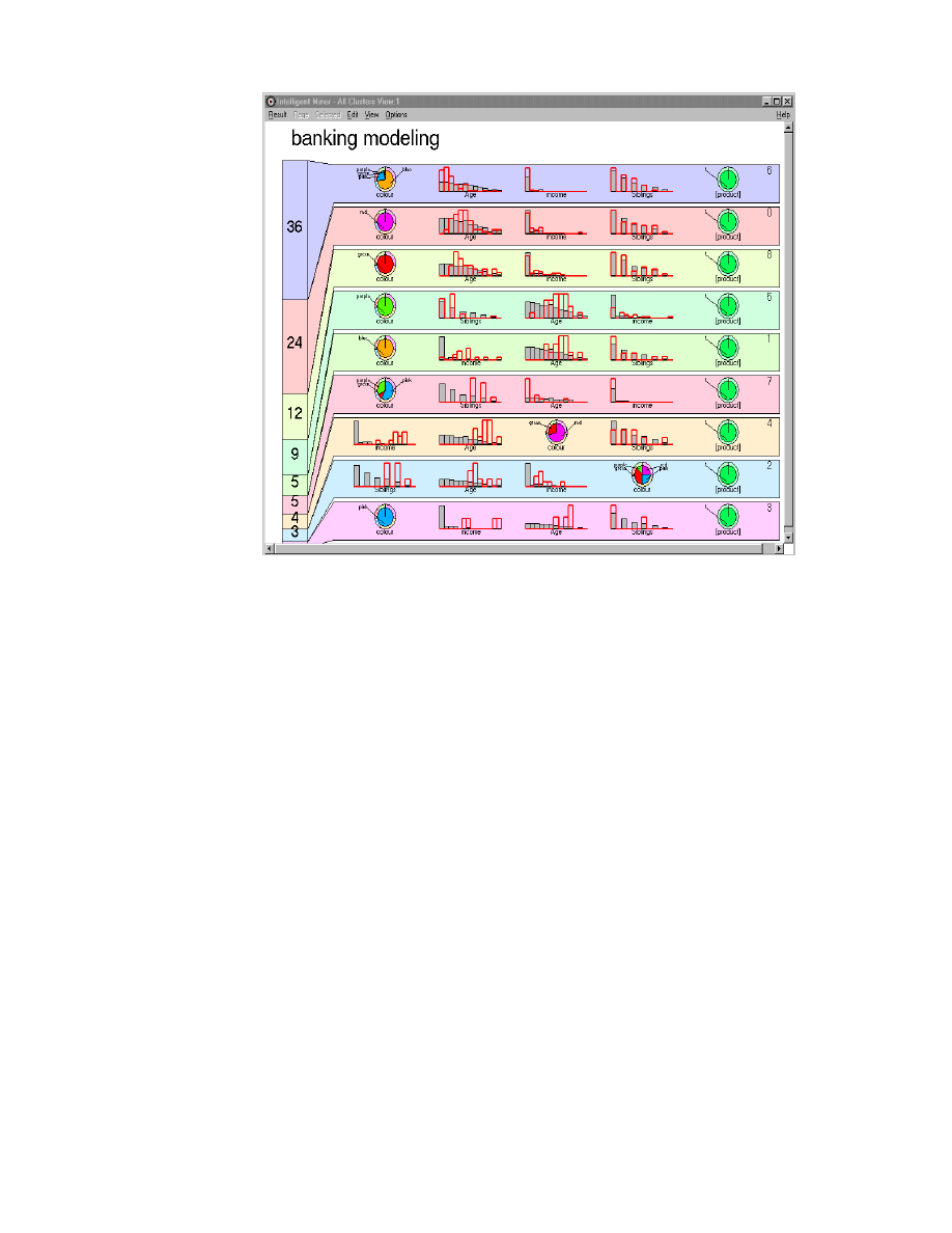
50
Getting Started with Data Warehouse and Business Intelligence
Figure 10. Sample Clustering Visualization
Result objects can be used in several ways:
• To visualize or access the results of a mining or statistical function
• To determine what resulting information you want to write to an output data
object
• As input when running a mining function in test mode to validate the
predictive model representation by the result
• As input when running a mining function in application mode to apply the
model to new data
3.4.8 Creating Data Mining Operations
The IM provides a means to construct data mining operations as a sequential
series of related data preparation, statistical, and mining functions. IM will
execute the objects in the order in which they have been specified. A
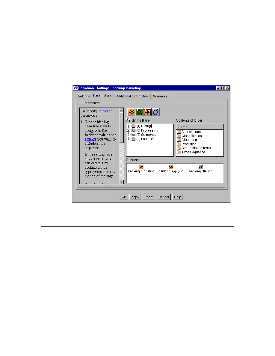
The Products and Their Construction
51
sequence can contain other sequences. You can construct standard
sequences that can be reused in similar data mining operations forming part
of a more complex sequence.
In IM, sequence setting objects are created through the sequence task guide.
You can select objects from the mining database and place them in the
sequence work area setting in the order in which they are to run. In addition
you can specify whether the sequence should continue if any of the setting
objects fails. Figure 11 illustrates a sequence-settings window.
Figure 11. Sequence-Settings Window
3.5 DB2 OLAP Server
The IBM DB2 OLAP Server is an online analytical processing (OLAP) server
that you can use to create a wide range of multidimensional planning,
analysis, and reporting applications. DB2 OLAP Server uses the Essbase
OLAP engine developed by Arbor Software Corporation. The OLAP Server
uses the Essbase engine for application design and management, data

52
Getting Started with Data Warehouse and Business Intelligence
access and navigation, data load, data calculation, and application
programming interfaces (APIs).
DB2 OLAP Server is compatible with Essbase, and can be used with all
Essbase-ready front-end tools and applications developed by Arbor and
Essbase partners.
DB2 OLAP Server allows you to:
• Perform multidimensional analyses on large volumes of relational data
• Manage data using relational database management system tools
• Access and query data in the star schema using standard SQL
statements.
DB2 OLAP Server replaces the integrated, multidimensional data storage
used by Arbor with a relational storage manager, and stores data in relational
data storage using a star schema.
The Relational Storage Manager (RSM) separates the OLAP engine from
database and provides support for DB2 and other relational databases.You
can manage the data stored by your Essbase applications using familiar
relational database management system (RDBMS) management, backup and
recovery tools.
Using the RSM, DB2 OLAP Server stores data in a relational database using
a star schema data structure, which means a fact table and a set of
dimension tables. The fact table holds the actual data values for the
database, and the dimension tables hold data about members and their
relationship.
You can access your data using Essbase clients, and you can access the
multidimensional data stored in the star schema using standard SQL
statements.
The RSM creates and manages automatically the necessary relational tables,
views and indices within the star schema, and the start schema can be
populated with calculated data to improve the performance of queries.
You can use DB2 OLAP Server with a new or existing DB2 database system.
If you plan to install a new DB2 database system, you can install DB2 OLAP
Server before or after you install DB2. You will need to collect specific
information about your DB2 system, such as database name, database user
ID, database password, and tablespace name, before you install DB2 OLAP
Server. This information can be collected from your DB2 database
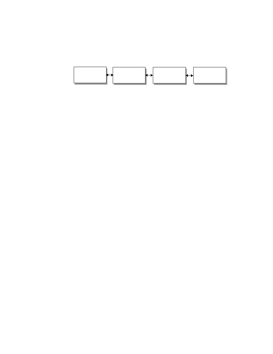
The Products and Their Construction
53
administrator, or you can configure the database information for DB2 OLAP
Server and then configure DB2 to match this configuration.
3.5.1 The General Architecture
In general, the architecture of an OLAP solution consists of the building
blocks depicted in Figure 12.
Figure 12. Architecture Building Blocks of an OLAP Solution
The Presentation Component provides a rich set of easy-to-use visualization,
navigation, and reporting capabilities that have contributed to the success of
OLAP tools in the marketplace.
The OLAP Engine is responsible for the multidimensional representation of
the model, the complex calculations, and the aggregations along the paths of
the dimension hierarchies.
The Data Store takes care of the persistency of the data represented in the
multidimensional model. It arranges the data elements of the model in a
physical structure for fast and efficient storage and retrieval.
Some solutions include an additional layer, the Application Component, which
typically resides between the presentation component and the
multidimensional calculation component. The application component
provides business logic that is targeted to a specific subject area (for
example, financial consolidation, marketing and sales support) and makes
use of the general functions provided by the multidimensional calculation
component.
3.5.2 Architecture and Concepts of DB2 OLAP Server and Essbase
Whereas Hyperion Essbase clearly belongs to the thin-client, two-tier,
M-OLAP category of available architectures, the positioning of the DB2 OLAP
Server within the defined categories is not so straightforward.
Both products shield the complexity of managing the data storage (that is, the
physical representation of the multidimensional model) from administrators
and users. The OLAP engine takes care of building and managing the actual
data store, based on the definition of the multidimensional model. Remember,
this is not the case for three-tier R-OLAP solutions, where the complex,
Presentation
Component
OLAP
Engine
Data
Store
Application
Component

54
Getting Started with Data Warehouse and Business Intelligence
time-consuming, and error-prone tasks of managing the data store and
defining the mapping information for the multidimensional calculation
component must be done by the administrator!
Whereas Hyperion Essbase is a pure M-OLAP solution (that is, it utilizes the
file system of the underlying operating system to store the data), DB2 OLAP
Server uses a standard DB2 Universal Database (UDB) to manage the
persistent model, and is, in this sense, an M-OLAP solution with relational
storage.
DB2 OLAP Server structures the data in a relational Star-Schema within DB2
UDB. The table structure in a star-schema is especially well suited for
multidimensional analysis of relational data. A star-schema consists of a
so-called fact table, which holds the numerical measures and key figures of
the business subject area. The fact table relates these measures to a number
of dimension tables, which contain the information to establish a context for
the recorded facts and hold the aggregation hierarchies to enable drill-down
and roll-up operations.
The elements of the dimensions are called members. They provide the
meaning for the numerical facts in the model and enable analysts to select
certain areas of interest by putting constraints on the attributes of the
dimension members. The members of a Market dimension are, for example,
all cities, where a company has sales outlets, such as Phoenix, San
Francisco, Los Angeles, San Diego. Members of the Market dimension
belonging to higher aggregation levels, such as states and sales regions are,
for example, California, Arizona and East, West. The members of these
higher levels summarize the facts related to the lower level members of the
dimension hierarchy.
Both Hyperion Essbase and DB2 OLAP Server share the exact same OLAP
engine, originally developed by Arbor Software Corporation. The OLAP
engine is accessed through an API, the Essbase API, which is also identical
between the two products. The Essbase API has established itself as a
common standard in the business intelligence industry. Many vendors
(more than 30, including Cognos and Business Objects, and Brio) have
implemented this API to provide access from their OLAP query products to
Hyperion Essbase and of course to DB2 OLAP Server.
The multidimensional calculation component retrieves and returns data
blocks from or to the data store component to satisfy the requests from the
client application. Therefore, in order to be able to use the same calculation
component for DB2 OLAP Server, the storage management component of
Hyperion Essbase, which deals with data blocks, had to be replaced by a

The Products and Their Construction
55
component to map the data blocks to the relational tables of the star-schema
and vice versa. This component is called the Relational Storage Manager
(RSM) in DB2 OLAP Server. It is also responsible for creating and
maintaining the tables, views, and indexes of the star-schema in DB2 UDB.
The architecture of DB2 OLAP Server combines the advantages of DB2 UDB,
the industrial-strength relational database management system, with the
power of the widely accepted Essbase OLAP engine, without putting the
burden of building and maintaining the relational data store on the
administrator. Furthermore, it enables database administrators to manage the
multidimensional data in the same way they manage relational data in the
data warehouse and in operational systems, thereby leveraging the skills,
utilities, and procedures already in place. The solution also integrates
smoothly into the existing backup strategy for relational data without
additional effort — for example, using ADSTAR Distributed Storage Manager
(ADSM).
Because the multidimensional data is stored in relational tables, it is also very
easy to do analysis across traditional relational data marts or data
warehouses and OLAP data marts, enabling a staged transition to OLAP
technology without losing analysis capabilities or introducing unnecessary
duplication of data.
Many standard reporting requirements can be solved with traditional
SQL-based decision support tools by directly accessing the star-schema of
DB2 OLAP Server without having to go through the Essbase calculation
engine.
Typically, in large business intelligence environments, both Hyperion Essbase
and DB2 OLAP Server are utilized. Consistency of the models, data, and
meta data exchange are managed by Visual Warehouse, which integrates
with both OLAP solutions.
Figure 13 compares the architectures of Hyperion Essbase and DB2 OLAP
Server.
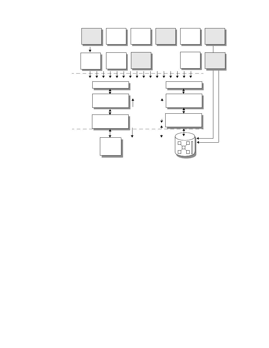
56
Getting Started with Data Warehouse and Business Intelligence
Figure 13. Hyperion Essbase and DB2 OLAP Server Architectures
As you can see in Figure 13, the OLAP Server functions can be accessed by
Essbase ready front-end tools that implement the Essbase API (such as
Hyperion Wired for OLAP or Cognos PowerPlay) and seamlessly integrated
in standard spreadsheets, such as Microsoft Excel and Lotus 1-2-3.
The administration interface for the OLAP Server is provided by the Essbase
Application Manager, which allows the definition of the models and the
initiation of the load and calculation processes.
Note that Figure 13 also includes the optional Essbase modules: Essbase
Adjustment Module, Essbase Currency Module, and Essbase Objects in the
Presentation and Application Components section. The Essbase Adjustment
Binary Files
Relational
Storage Manager
Essbase OLAP
Engine
Essbase OLAP
Engine
Essbase API
Essbase
Application
Manager
Essbase
Spreadsheet
Add-in
Essbase
Front-End
Star-Schema
relational
DB2 UDB
NT or UNIX
File System
Essbase API
Ready
Tools
MS Excel,
Lotus 123
Hyperion Essbase
DB2 OLAP Server
SQL Decision
Support
Applications
RDBMS
Management
Tools
Da
ta
B
lo
c
k
s
SQ
L
Da
ta
B
lo
c
k
s
OL
A
P
E
ngi
n
e
Da
ta
S
to
re
P
re
sen
ta
ti
o
n
an
d
A
p
p
licat
io
n
Co
m
p
o
n
e
n
ts
Essbase
Currency
Module
Essbase
Adjustment
Module
Essbase
Objects
Multidimensional
Storage Manager
Essbase
Web
Gateway
Hyperion
Integration
Server
Define/Load/Calculate

The Products and Their Construction
57
Module provides a complete application for financial consolidation. The
Essbase Currency Module contains the functions for currency conversions.
The Essbase Objects provide ActiveX components for all major Essbase
functions, which can easily be integrated in custom applications,
implemented in, for example, Visual Basic or C++.
3.5.3 Supported Platforms and RDBMSs
You can run DB2 OLAP Server on the following platforms:
• OS/2 Warp Version 4.0 or later
• Windows NT Version 4.0 or later
• AIX Version 4.2 or later.
DB2 OLAP Server supports these RDBMSs:
• DB2 Universal Database (UDB) Version 5 Workgroup Edition or later
• DB2 Universal Database (UDB) Version 5 Enterprise Edition or later
• DB2 Database Server Version 4.0.1
• DB2 Common Server Version 2.1.2
• DB2 for OS/390 Version 4.1 or later
3.5.4 Wired for OLAP Server
The OLAP database can be used from end user tools such as Wired to work
with the multidimensional database and initiate analytical queries using
drag-and-drop.
Wired for OLAP is an OLAP-centric analysis and presenting tool that
operates in both client/server and Web-based computing architectures.
Wired for OLAP delivers:
• Highly graphical displays
• Intuitive OLAP navigation
• Robust analytics
• Analytical collaboration
• Easy customize and extend

58
Getting Started with Data Warehouse and Business Intelligence
3.6 DB2 Connect
DB2 Connect, a member of IBM's industry-leading DB2 Universal Database
family of products, is IBM's successor to IBM's Distributed Database
Connection Services (DDCS).
DB2 Connect provides extremely fast and robust connectivity to IBM
mainframe databases for E-business and other applications running under
the following Intel and UNIX operating systems:
• AIX
• HP-UX
• Microsoft Windows (all variants)
• OS/2
• Sun Solaris
DB2 Connect is supported by the following IBM database products when
running as DRDA Application Servers:
• DB2 for AS/400 Version 2.1.1 or higher
• DB2 for MVS/ESA Version 3.1 and Version 4
• DB2 for OS/390 Version 5 or higher
• DB2 Common Server Version 2
• DB2 Universal Database Version 5 or higher
• SQL/DS Version 3.5
• DB2 for VSE & VM Version 5 or higher
Connectivity to host databases is provided over Systems Network
Architecture (SNA) connections using IBM's Advanced Peer-to-Peer
Connection (APPC) network protocol for DB for AS/400, DB2 for MVS, DB2
for OS/390, DB2 for VM & VSE, and SQL/DS. DB2 for OS/390 also supports
database connections over TCP/IP.
DB2 Connect is available in two forms:
1. DB2 Connect Enterprise Edition (see Figure 14).
DB2 Connect Enterprise Edition supports Intel and UNIX workstations in a
workgroup, department or LAN setting.
Operating systems supported:
• AIX
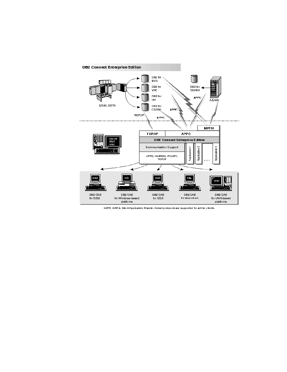
The Products and Their Construction
59
• HP-UX
• OS/2
• SCO UnixWare
• Solaris
• Windows NT
Figure 14. DB2 Connect Enterprise Edition
2. DB2 Connect Personal Edition (see Figure 15).
DB2 Connect Personal Edition is intended for single-users on Intel
workstations.
Operating systems supported:
• OS/2
• Windows 3.1
• Windows 3.11 for Workgroup
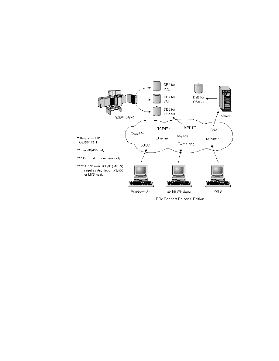
60
Getting Started with Data Warehouse and Business Intelligence
• Windows 95
• Windows 98
• Windows NT
DB2 Connect Personal Edition includes Integrated SNA Support for use
on Windows 3.1, Windows 3.11 for Workgroup, and Windows 95. Users of
OS/2 also require IBM Communications Server for OS/2. Users of
Windows NT also require IBM Communications Server for Windows NT, or
Microsoft SNA Server Version 2.11 or higher.
Figure 15. DB2 Connect Personal Edition
DB2 Connect Version 5.2 includes the following enhancements for the host
and AS/400 DRDA functions.
• DCE Cell Directory support
Users working with host and AS/400 databases servers now have
additional options for providing database location information when using
DCE Cell Directory support for implementations from IBM and Gradient.
Refer to the Administration Guide for additional information.
• Enhanced password management

The Products and Their Construction
61
DB2 Connect now permits users to change their passwords without having
to log on to their database server. Users can now change their passwords
in any one of four ways: by using the SQL CONNECT statement from the
DB2 Command Line Processor, by requesting a password change from
within the ODBC login dialog, by using the password change option of the
Client Configuration Assistant, or by using the ATTACH command.
In addition, application programmers can now take advantage of DB2
Connect enhanced password management to deliver more robust security
mechanisms for their applications. The ability to change user passwords is
provided for Embedded SQL, ODBC, and DB2 CLI, as well as for Java
using both JDBC and SQLJ.
For example, with this support, a user connected to a DB2 for OS/390
database server no longer has to sign on to TSO in order to change his or
her password when it expires. Through DRDA, DB2 for OS/390 can
change the password for you. The old password along with the new
password and the verify password must be supplied by the user.
If the security specified at the DB2 Connect EE gateway is DCS, then a
request to change the password is sent to the DRDA server. If the
authentication specified is SERVER, then the password on the gateway
machine is changed.
An additional benefit is that, with TCP/IP connections to the host, a
separate LU definition is no longer required, as was the case with DB2
Connect Version 5.0. Refer to the manual, DB2 Connect Enterprise
Edition Quick Beginnings, S10J-7888, for additional information.
• Enhanced security failure notification
Users connecting to host and AS/400 databases can now get additional
information on the cause of security failures when they occur, for example
as the result of an expired password. Refer to the manual, DB2 Connect
Quick Beginnings, S10J-7888, for further information.
In addition, password change support is now supported through DRDA
(see Enhanced password management above).
• Enhanced System/390 SYSPLEX exploitation
DB2 Connect Enterprise Edition (EE), and the DB2 Connect component
that is included in both DB2 UDB EE and DB2 UDB Extended - Enterprise
Edition (EEE), can now provide enhanced load balancing and fault
tolerance by routing connections to different nodes on a System/390
SYSPLEX. Some additional configuration considerations apply, and these
are documented in the manual, DB2 Connect Enterprise Edition Quick
Beginnings, S10J-7888.

62
Getting Started with Data Warehouse and Business Intelligence
• Optimized Catalog Access for ODBC and JDBC Applications
A new tool db2ocat is provided on Windows 32-bit operating systems in
order to assist customers to optimize system catalog searches for ODBC
applications.
DB2 Connect now offers a way to dramatically improve the performance of
ODBC and JDBC applications that make extensive use of the system
catalog. This improvement is provided using the CLISCHEMA parameter
in the DB2CLI.INI file, which allows applications to use an
ODBC-optimized catalog instead of the regular system catalog tables. In
addition, a point-and-click utility that greatly simplifies the creation and
maintenance of ODBC-optimized catalogs can be obtained by
downloading db2ocat.zip from:
ftp://ftp.softwre.ibm.com/ps/products/db2/tools
• Microsoft Transaction Server support
DB2 family databases including host and AS/400 databases can now fully
participate in distributed transactions managed by the Microsoft
Transaction Server (MTS). Refer to the DB2 Connect Enterprise Edition
Quick Beginnings, S10J-7888 for additional information.
• New BIND options (DYNAMICRULES)
There are two new enumerated values for the DYNAMICRULES option of
the BIND command. These two values: DEFINE, and INVOKE, are
defined to specify the authorization identity to be used for the execution of
a dynamic SQL statement in a user defined function (UDF) or in a stored
procedure:
• DEFINE
Indicates that the authorization identifier used for the execution of
dynamic SQL is the definer of the UDF or stored procedure.
• INVOKE
Indicates that the authorization identifier used for the execution of
dynamic SQL is the invoker of the UDF or stored procedure. Refer to
the IBM DB2 Universal Database Command Reference, S10J-8166, for
further information.
• Set Client Information API enhancements
A new Set Client Information API allows three-tier client/server or TP
monitor applications to pass more specific information about the
application end user to DB2 for OS/390.

The Products and Their Construction
63
The new information includes the end user name supplied by server
application, the workstation name, the application name, and the
accounting string. This information can now be reported by the DB2 for
OS/390 DISPLAY THREAD command, and it is available in DB2 for
OS/390 accounting records. Previously, in three-tier environments, DB2
for OS/390 could only provide information about the server application and
the individual authentication user ID, and not about the numerous end
users who multiplex SQL queries on long-running connections. For
additional information, refer to the IBM DB2 Universal Database API
Reference, S10J-8167.
• SQLDescribeParam support for DB2 Connect
With this enhancement, an application is now able to issue the
SQLDescribeParam API call to retrieve parameter descriptions from a
DB2 for OS/390 data source.
• Support for Bidirectional Languages
DB2 Connect now provides support for bidirectional languages such as
Arabic and Hebrew. Refer to the IBM DB2 Universal Database
Administration Guide, S10J-8157, for more information about the nature of
this support.
For information on configuring DB2 Connect Version 5.2 for bidirectional
languages please refer to the Release Notes for DB2 Connect Version 5.2,
provided with the product.
• System Monitor enhancements
The following System Monitor enhancements for DB2 Connect are
provided in Version 5.2:
• Enhancements to the sqlmonss API call and the LIST DCS
APPLICATIONS command provide for the listing of seven new data
elements: DCS application status, client login ID, client platform, client
protocol, host CCSID, process ID of client application, and status
change time.
• New GET SNAPSHOT support for DB2 Connect at the database
manager and application levels, where the application level reporting
includes statement and transaction levels.
• New SNAPSHOT support for DB2 Connect at the database level.
Information about detailed updates to the System Monitor Guide and
Reference, S10J-8164, is contained in What's New.
• Two-phase commit support enhancements

64
Getting Started with Data Warehouse and Business Intelligence
In DB2 Connect Enterprise Edition Version 5.0, two-phase commit support
over SNA connections using the DB2 Syncpoint Manager (SPM) was only
available on AIX and OS/2. With DB2 Connect Enterprise Edition Version
5.2, this support is now extended to Windows NT. This support requires
IBM eNetwork Communications Server for Windows NT Version 5.01 or
higher.
Two-phase commit for XA applications was previously only supported over
SNA connections, using the SPM. It is now also supported over TCP/IP
connections using the SPM.
Applications executed by Transaction Processing Monitors such as IBM
TXSeries, CICS for Open Systems, Encina Monitor, and Microsoft
Transaction Server previously had to access host systems such as DB2
for OS/390 using SNA. With DB2 Connect Version 5.2, TCP/IP can now be
used by these same applications. The DB2 Syncpoint Manager must be
used to enable this new feature.
For further information refer to the manual, DB2 Connect Quick
Beginnings, S10J-7888.
• Simplified DB2 Syncpoint Manager Configuration
DB2 Syncpoint Manager configuration has been simplified. Many steps
are now automated or eliminated compared to previous releases. Please
refer to the manual, DB2 Connect Quick Beginnings, S10J-7888.
• Support for the SCO** operating system
DB2 Connect Enterprise Edition Version 5.2 is available for the SCO
operating system.
• Support for Big Integer, Large Object, Row ID, and User Defined Distinct
data types.
DB2 Connect Version 5.2 now provides support for Big Integer, Large
Object, Row ID, and User Defined Distinct data types. Refer to the IBM
DB2 Universal Database SQL Reference, S10J-8165, for more details.
• Enhancements to the Client Configuration Assistant
In V5.2 you can use the Client Configuration Assistant (CCA) to configure
TCP/IP connections to DB2 for VM and DB2 for AS/400 database servers.
You can also use the CCA to configure IBM Communications Server for
NT (CS/NT) and IBM Personal Communications (PComm) SNA stacks if
you are using an SNA network.

The Products and Their Construction
65
3.7 IBM e-Network Communication Server Host-on Demand
This section describes the IBM e-Network Communication Server product
that has to be used when the connectivity between the workstation platforms
and the host system must be established using the APPC networking protocol
rather than the TCP/IP protocol.
3.7.1 Communication Server
The solution for a changing environment IBM Communications Server, part of
the IBM Software Servers line, meets the challenge of today's changing
business environment. Communications Server offers Internet and intranet
solutions that allow your company to take advantage of network computing
advances—like information access, electronic commerce, and collaboration.
With Communications Server, you choose applications based on your
business needs, not on your network. With various local area networks
(LANS), mergers, consolidations, and changes to organizational structure, is
your network still able to connect applications, data, and people-regardless of
where they are? Communications Server brings you true networking,
interconnecting people and applications, even when platforms and network
configurations are diverse.
Communications Server brings you the reliability, open standards, scalability,
and security you've come to expect from IBM. Communications Server is the
solution to meet your needs, today and tomorrow.
The Communications Server is designed to meet your networking
requirements, so you can concentrate on making your business a success.
Communications Server lets workstation users and applications communicate
with other workstations and large-computer applications, enabling commerce,
encouraging collaboration, and managing your content. The Communications
Server provides easy access to the information and people you need in
today's diverse multiprotocol network computing environment.
It belongs to the IBM Software Server products, that also include:
• IBM DATABASE 2 (DB2) Database Server
• IBM Directory and Security Server
• IBM Internet Connection Server
• Tivoli Management Server
• IBM Transaction Server
• Lotus Domino Server

66
Getting Started with Data Warehouse and Business Intelligence
3.7.1.1 Highlights
• Make application decisions based on business needs, not network
protocols
• Access the information you need—when you need it—from a large
computer or LAN, whether you are in the office or on the road
• Discover a powerful gateway server for SNA and TCP/IP clients
• Improve your network systems management through consolidated traffic
and reduced need for parallel networks
• Enable remote, integrated cross-server administration capability through
the Web
• Get the widest range of connectivity in the industry
• Provide TCP/IP users access to 3270 central computer applications
through TN3270E server
• Provide easy SNA 3270 application access from any Java-enabled Web
browser
3.7.1.2 Web-Based Server Administration
Communications Server provides a new Web-based tool that gives you
remote integrated cross-server administration capability. IBM takes
Web-based server administration to a new dimension. A simple graphical
user interface provides a convenient, at-a-glance status of Communications
Server, while a user interface that is consistent across server platforms
preserves a common look and feel.
3.7.1.3 A Solution
Communications Server is the solution for companies that:
• Need to expand the use of applications, yet protect current network
investments
• Need to reduce operation and management costs by connecting networks
without impacting existing applications
• Must reduce costs of central computer systems and peer-to-peer
connectivity by sharing communication resources
• Want to improve network availability and response time by assigning
priority to short, interactive data transmissions rather than to
batch-oriented bulk data traffic

The Products and Their Construction
67
3.7.1.4 Protocol Independence
The Communications Server opens the door to protocol-independent
networking, with seamless support for workstations communicating across
SNA, IPX, NetBIOS, and TCP/IP networks. This interoperability gives you the
freedom to be responsive to changing business applications, without
disrupting your network. Delivering data where it is needed, when it is
needed, is a fundamental challenge in today's networked environment.
Communications Server lets you exploit the newest technology to maintain
your competitive edge.
The Communications Server provides powerful, multiprotocol gateway
support for SNA, TCP/IP, IPX, and NetBIOS networks. Communications
Server connects applications on many platforms across heterogeneous
networks. AnyNet technology, based on open standards, provides the
capability to run sockets TCP/IP applications over SNA; SNA applications
over TCP/IP; and, with Communications Server for OS/2, you can run IPX- or
NetBIOS-applications over TCP/IP and SNA networks. You can mix and
match SNA and TCP/IP-based network protocols as you expand or combine
networks.
Applications written for SNA, sockets, IPX, or NetBIOS can run without
change on mixed network backbones. For diverse networks, Communications
Server gives you the breadth of function, connectivity, and capacity to support
future needs.
Communications Server also provides TN3270E server function. This allows
TCP/IP users easy access to 3270 applications. With the standard
extensions, users can print to their workstations or to printers in the TCP/IP
network. Also, requesting a resource (LU or pool of LUs), responses, and Attn
and SysReq keys are supported. TN3270E support is compliant with industry
standard Request For Comment (RFC) 1576, RFC 1646, and RFC 1647. This
function is integrated as part of the Communications Server for OS/2 and
Windows NT. For Communications Server for AIX, this function is provided by
SNA Client Access for AIX (an optional licensed program). SNA Client
Access also includes TN5250 server support and dynamic load-balancing
capabilities.
3.7.1.5 Mobile Computing
With the IBM Communications Server and a laptop computer, you can take
your applications on the road. In addition, remote personal computers can
easily access information on central computer systems and other personal
computers attached to a LAN. Either way, you gain productivity by staying
connected in today's mobile work environment.

68
Getting Started with Data Warehouse and Business Intelligence
3.7.1.6 SNA Services
The Communications Server provides all-in-one SNA communication
services from workstations to an S/390 system, an AS/400 system, or other
workstations. Its capabilities include a full-function SNA gateway, the most
Advanced Peer-to-Peer Networking in the industry, support for many types of
connections, and a rich set of application programming interfaces (APIs). Of
particular significance is the support of SNA, which is based on IBM's long
experience as the architect and developer of this important networking
protocol.
3.7.1.7 Advanced Peer-to-Peer Networking
Communications Server acts as a subarea node and an Advanced
Peer-to-Peer Networking (APPN) node (both network node and end node).
Communications Server APPN support includes SNA networking facilities
that connect distributed computing applications, peer applications, and client
applications to their servers.
The Communications Server also includes support for High-Performance
Routing (HPR), which improves availability and throughput for network
communication. It provides error recovery, connection awareness,
sophisticated flow control, and segmentation at the end points of a
connection, freeing intermediate nodes to move data.
On the Communications Server for OS/2 or Windows NT, if an intermediate
link or node in a connection route fails, HPR can Determine a new connection
route and resume transmission without disrupting your users' sessions.
3.7.1.8 Supported Platforms and Functions
IBM Communication Server is available for the following operating systems:
• OS/390
• AIX
• DOS
• OS/2
The IBM Communications Server for OS/2 Warp provides two freestanding
components that can be licensed and installed separately to support
application development in OS/2 or Windows environments. These
components provide SNA services and application programming
interfaces for LAN-attached workstations and can function independently
from the Communications Server for OS/2 Warp gateway server.
OS/2 Access Feature consists of 32-bit and 16-bit APIs, LAN and WAN
connectivity, APPN end node, and multiprotocol support for the desktop.

The Products and Their Construction
69
This allows Sockets applications over SNA and SNA applications over
TCP/IP to communicate with each other through the multiprotocol
gateway.
• Windows 3.1, Windows95, Windows NT
Windows Access Feature consists of the APPC Networking Services for
Windows product (NS/Windows) and the multiprotocol support, which lets
APPC and CPI-C applications communicate through the SNA over TCP/IP
gateway to IBM and other computers. NS/Windows provides the CPI-C
application programming interface and APPC support for APPN low-entry
network (LEN) end node.
The Communication Server provides the following functions:
• SNA over TCP/IP and Sockets over SNA network communication
• Features APPN network node, end node, including support for HPR and
dependent LU requester (DLUR)
• Delivers a rich set of APIs to develop applications for distributed
computing, including support for APPC, Common Programming Interface
for Communications (CPI-C), and LUA
• Supports TN3270E server functions
• Enables easy 3270 SNA access to any Java-enabled Web browser with
Host On-Demand
• Accommodates a broad range of LAN and wide area network (WAN)
protocols, including Fiber Distributed Data Interface (FDDI), Synchronous
Data Link Control (SDLC), asynchronous transfer mode (ATM), and X.25.
The OS/2 and Windows NT Servers also support integrated services
digital network (ISDN), integrated data link control (IDLC), and frame relay
• Provides S/390 channel and ESCON support with efficient, high-capacity
access to multiple large computers (available for AIX and Windows NT)
• Offers remote access to SNA applications over asynchronous,
synchronous, Hayes AutoSync, digital, and cellular connections
• Supports a wide range of IBM and OEM adapters and modems
• Remote installation and configuration
• Allows easy-to-use Web-based, remote cross-server administration
Communications Server for Windows NT allows TCP/IP-attached clients to
access SNA APIs, without requiring SNA protocols to flow between the clients
and the server. This allows most SNA configuration to take place at the
central server. Communications Server supports SNA API clients on Windows

70
Getting Started with Data Warehouse and Business Intelligence
95, Windows NT, Windows 3.1, or higher, and OS/2. With this configuration
the server handles the processing while reducing the storage and workload at
the client PCs.
3.7.1.9 Benefits
Everyone benefits from the Communications Server:
• Users have a wider choice of new applications, because the
Communications Server expands the reach of existing applications.
Applications can be deployed to all users quickly and economically.
• Administrators can focus on optimizing the network environment for
availability and response time, confident they are always ready to support
new application requirements and can still manage costs.
• Application writers can select the APIs they use, based on functions the
API provides, without regard to the underlying network. Existing
applications can be run over additional network types, expanding the
market for those applications. In this way, application providers can
concentrate on improving their products rather than on developing
different versions to run on different protocols.
3.7.2 Host-on Demand
IBM eNetwork Host On-Demand is an Internet-to-host interconnectivity
solution that provides host application access through the Web.
Web users needing host applications, such as public catalogs, databases,
and other resources, can use eNetwork Host On-Demand from inside their
Java-enabled Web browsers to access central computer data.
eNetwork Host On-Demand delivers network computing to the Web by
enabling Web browser users seamless access to non-Internet-based 3270,
5250, ASCII, and CICS Gateway for Java applications, content, and
services.This product, available in a single package, can run in any
Java-enabled environment. Thus you have simple and consistent access to
your enterprise data, and the need for user installation, user configuration,
and costly software upgrade administration is eliminated.
eNetwork Host On-Demand is Java-based, so users in different operating
environments—whether they are using network computers, traditional
personal computers, or advanced workstations—get the same look and feel.
This consistency reduces retraining costs when users change operating
environments, and it reduces service costs, because each user is on the

The Products and Their Construction
71
same version of the code. You can extend the reach of your enterprise data
and applications by using eNetwork Host On-Demand's SSL authentication
and encryption to gain secure access across the Internet.
eNetwork Host On-Demand Version 2.0 also provides many features that
enable users to customize the interface and to transfer data to other desktop
applications. File transfer, cut and paste, and print screen are included to
increase user productivity. A Java-based API for application development is
available to customize desktops. National language versions are also
available, including versions for double-byte character sets and file transfers.
Host On-Demand includes the following components:
• Server
The server must be installed on a Web server. It includes a client that can
be downloaded to workstations, and an administration function that can be
used, through a browser, on the server itself or on a client workstation.
• Redirector
The Redirector allows a client to connect to multiple Telnet servers (or
host systems) even if it is using a browser that does not support signed
Java applets. It also allows the use of SSL Version 3 security between
clients and the server. The Redirector is part of a server installation.
• Express Server
The Express Server, together with the Express Client, provides enhanced
performance on slower connections, such as telephone lines. It also
provides redirection function and SSL support. The Express Server is part
of a server installation.
• Download client
The Host On-Demand emulator applet is downloaded to a workstation
from a Host On-Demand server, through a Web browser. Most common
browsers can be used. No program files are installed on the workstation.
Unless the browser supports signed Java applets, the client can connect
to host systems only through the server from which it was downloaded.
The client supports SSL security. It is part of a server installation.
The user of a download client has three possible ways of working:
• As a defined user, with an ID and password, and a host-session profile
that is unique to that user. The user account and session profile are
saved on the server.
• As a guest user, who uses the default host-session profile.

72
Getting Started with Data Warehouse and Business Intelligence
• With the simple user interface (SUI). The SUI is similar to the interface
provided with Host On-Demand Release 1, and has minimal
configuration capability.
• Locally installed client
This client supports SSL security. The user of a local client has two
possible ways of working:
• Full-function
All four types of host sessions can be used concurrently, and session
definitions are saved on the local disk.
• SUI
Again, the SUI is similar to the interface provided with Host
On-Demand Release 1.
Both the download client and the locally installed client can use the Host
Access Class Library API. Message logging and tracing are provided on
clients and the server.
More information on eNetwork Host On-Demand is available at:
http://www.software.ibm.com/enetwork/hostondemand
3.8 Net.Data and Its Architecture
Net.Data is a Web server gateway that application developers can use to
create Internet applications that access data from IBM’s DB2 family
databases. It enables an application developer to build Web applications that
access DB2 databases by using HTML forms and dynamic SQL. These
applications are then stored on the Web server, and the end user can use any
Web browser to access the HTML forms returning DB2 data.
Net.Data builds on the strengths of its predecessor product, DB2 World Wide
Web Connection (DB2WWW), in enabling interactive, data-rich sites. As
such, IBM Net.Data delivers a powerful framework for Web applications. In
addition to connecting to diverse data sources, Net.Data provides for high
performance, robust application development function, and exploitation of
existing business logic.
Net.Data provides native access to the data you need in your business
environment: DB2, as well as Oracle, IMS, and file data. In addition, through
ODBC you can access many other relational data sources. And, Net.Data
optimizes access to advanced objects in the DB2 family such as DB2 stored
procedures.

The Products and Their Construction
73
By tightly integrating with specific Web server interfaces (such as GWAPI),
Net.Data can operate as an extension of the Web server, delivering improved
performance over CGI applications. Net.Data provides high-performance
access to all of your data sources, including hot connectivity to your DB2 data
sources.
Net.Data has extensive application development functionality. A rich macro
language, conditional logic, HTML and Virtual Reality Modeling Language
(VRML) support, HTML variable substitution, a JDBC interface to DB2 data,
and support for multiple data sources result in flexible yet robust Web
applications.
You can repurpose your existing client/server applications to the Web, using
your existing business logic, embed dynamic SQL, Java applets and
JavaScripts, Perl and REXX in your Net.Data application, or call DLLs written
in C or C++. By leveraging your existing business applications, you can get
your Web applications up and running quickly with Net.Data.
Net.Data is architected as a program that is called by a Web server through
either the CGI, ICAPI, or GWAPI (see Figure 16). The Net.Data application
uses macro file containing sections, text, HTML, SQL to be executed,
programs and scripts to be called, and application control logic. It uses these
directives in the macro file to interpret the input from the browser and the
Web server, access the specified data sources, and generate the requested
output to the browser.
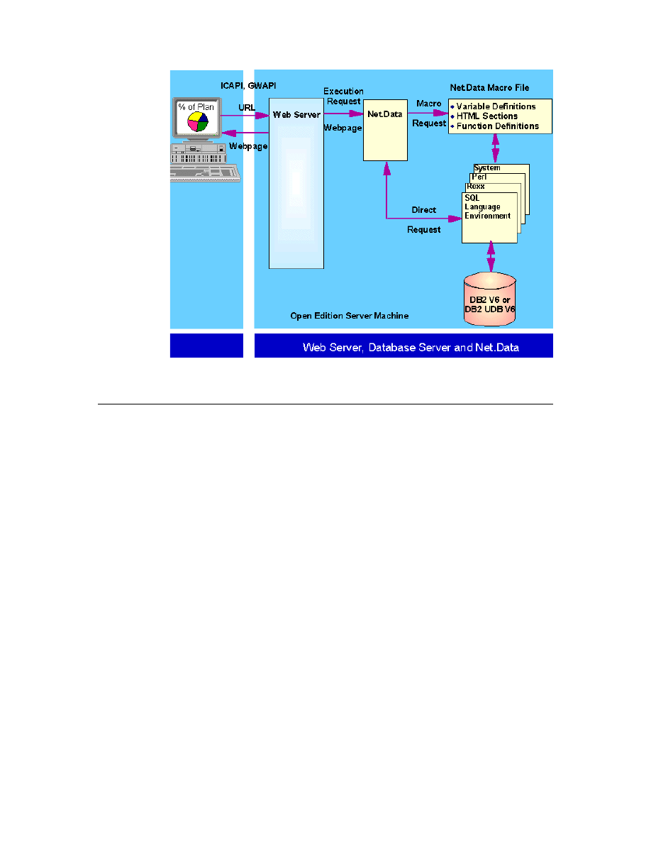
74
Getting Started with Data Warehouse and Business Intelligence
Figure 16. Net.Data Architecture
3.9 Web Server
Web content is what you provide your users from your Web server. Content
could include general information about your enterprise, advertising,
descriptions of products and services, and order entry facilities.
Two interface options are available for Web programming:
• CGI—where a process is created and destroyed on each Web click.This
option is much too expensive to consider for high volume applications.
• All other interfaces (for example, GWAPI, servlets, and FastCGI)—These
interfaces provide better performance. However, there is a price to pay:
You have to do more of the work. For example, with servlets, FastCGI, or
GWAPI, none of the system components is responsible for data integrity or
SQL state on your behalf. Typically, these interfaces allow you to establish
a database connection and then reuse the connection over multiple Web
requests.

The Products and Their Construction
75
However, if you make a mistake in your application, there is no automatic
cleanup mechanism. For example:
• You might run your program to completion, but forget to issue COMMIT.
• You might take an exception and then fail to catch the error (that is, you
did not retry out of the exception).
• You might set the SQL special registers to some unexpected values during
one Web request. If you do not remember to reset the registers, the next
Web request will inherit whatever you have left behind.
The basic problem here is that the Web does not behave like IMS, CICS, or
DB2 stored procedures, where the system watches for application errors and
cleans up as needed. The Web does not do anything special for SQL access,
so you have to manage the cleanup on your own. Net.Data provides some of
this "safety net" function for your application.

76
Getting Started with Data Warehouse and Business Intelligence

© Copyright IBM Corp. 1999
77
Chapter 4. Data Communication
In data communication, several layers of communication are used in a very
complex environment connecting different operating systems and data
sources of completely different architectures.
From the application point of view, the base for all communication and data
transfer consists of the communication protocols. Several protocols are
available for inter-system communication. Especially in the workstation area,
you have several options.
• The connectivity between the workstation environment and the host
systems is based, for example, on Ethernet or on Token Ring.
• The communication protocols mostly used in the workstation environment
are NetBIOS and TCP/IP. TCP/IP is used for communication to the host
systems as well.
• The most common protocol in the host environment is still APPC
(Advanced Program to Program Communication) based on SNA (Shared
Network Architecture). The usage of APPN (Advanced Peer to Peer
Networking) simplifies the configuration.
• Whether APPC or TCP/IP is used for the communication with the host
systems depends on the capabilities of the communication partner on the
host side. For example, Cross Access for VSE can use both protocols,
whether DB2 Server for VSE V 5.1 uses APPC only.
The next layer is the protocol or architecture supplying the base for the
data exchange between the data sources and targets.
• For the data transfer between DB2 family products and other relational
database software in different operating environments (host and
workstation) it is DRDA (Distributed Relational Database Architecture).
• But between like platforms (workstations or VM and VSE) there are
so-called private protocols available as well. For example, between the
Universal Databases (UDBs) on the workstations, there is a private data
exchange protocol available, which has the same functionality as DRDA.
• For the nonrelational data sources, there exist special ’private’ solutions
(like CrossAccess or Classic Connect) used to provide these sources in a
relational view.

78
Getting Started with Data Warehouse and Business Intelligence
4.1 Communication Protocols
The following sections provide a description of the possible communication
protocols you can choose for your implementation. Understanding how they
work and what they need, you can identify which solution fits best in your
environment.
4.1.1 TCP/IP
The need to interconnect networks that use different protocols was
recognized early in the 1970s during a period when both the use and
development of networking technology were increasing. Even though the
rapid growth in networking over the past three decades has allowed users
much greater access to resources and information, it has caused significant
problems with merging, or interconnecting, different types of networks. Open
protocols and common applications were required, leading to the
development of a protocol suite known as Transmission Control
Protocol/Internet Protocol (TCP/IP), which originated with the U.S.
Department of Defense (DoD) in the mid-1960s and took its current form
around 1978.
An interesting article about the history of the Internet can be found at:
http://www.isoc.org/internet-history/
In the early 1980s, TCP/IP became the backbone protocol in multivendor in
networks such as ARPANET, NFSNET, and regional networks. The protocol
suite was integrated into the University of California at Berkeley's UNIX
operating system and became available to the public for a nominal fee. From
that point TCP/IP became widely used. Its spread to other operating systems
resulted in increasing use in both local area network (LAN) and wide area
network (WAN) environments.
Today, TCP/IP enables corporations to merge differing physical networks
while giving users a common suite of functions. It allows interoperability
between equipment supplied by multiple vendors on multiple platforms, and it
provides access to the Internet. In fact, the Internet, which has become the
largest computer network in the world, is based on TCP/IP.
So why has the use of TCP/IP grown at such a rate? The reasons include the
availability of common application functions across differing platforms and the
ability to access the Internet, but the primary reason is that of interoperability.
The open standards of TCP/IP allow corporations to interconnect or merge
different platforms. An example is the simple case of allowing file transfer

Data Communication
79
capability between an MVS/ESA host and, perhaps, a Hewlett Packard
workstation.
TCP/IP also provides for the routing of multiple protocols to and from diverse
networks. For example, a requirement to connect isolated networks using
IPX, AppleTalk, and TCP/IP protocols using a single physical connection can
be accomplished with routers using TCP/IP protocols.
One further reason for the growth of TCP/IP is the popularity of the socket
programming interface between the TCP/IP transport protocol layer and
TCP/IP applications. A large number of applications today have been written
for the TCP/IP socket interface.
4.1.1.1 TCP/IP Architecture
TCP/IP, as a set of communications protocols, is based on layers. Unlike
System Network Architecture (SNA) or Open Systems Interconnection (OSI),
which distinguish seven layers of communication, TCP/IP has only four
layers. See Figure 17. The layers enable heterogeneous systems to
communicate by performing network-related processing such as message
routing, network control, and error detection and correction.
• Application Layer
The application layer is provided by the program that uses TCP/IP for
communication. Examples of applications are Telnet, File Transfer
Protocol (FTP), e-mail, Gopher and SMTP. The interface between the
application and transport layers is defined by port numbers and sockets.
• Transport Layer
The transport layer provides communication between application
programs. The applications may be on the same host or on different
hosts. Multiple applications can be supported simultaneously. The
transport layer is responsible for providing a reliable exchange of
information. The main transport layer protocol is TCP. Another is User
Datagram Protocol (UDP), which provides a connectionless service in
comparison to TCP, which provides a connection-oriented service. That
means that applications using UDP as the transport protocol have to
provide their own end-to-end flow control. Usually, UDP is used by
applications that need a fast transport mechanism.
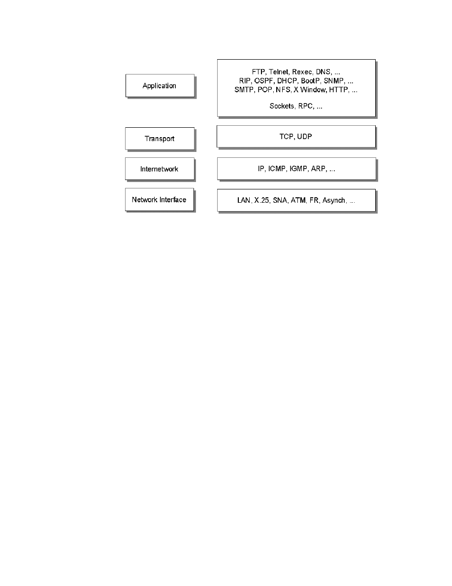
80
Getting Started with Data Warehouse and Business Intelligence
Figure 17. TCP/IP Architecture Model: Layers and Protocols
• Internet Layer
The Internet layer provides communication between computers. Part of
communicating messages between computers is a routing function that
ensures that messages will be correctly delivered to their destination. The
Internet Protocol (IP) provides this routing function. Examples of Internet
layer protocols are IP, ICMP, IGMP, ARP and RARP.
• Network Interface Layer
The network interface layer, sometimes also referred to as link layer, data
link layer or network layer, is implemented by the physical network that
connects the computers. Examples are LAN (IEEE 802.x standards),
Ethernet, X.25, ISDN, ATM, Frame Relay, or asynch.
Note that the RFCs actually do not describe or standardize any network
layer protocols by themselves, they only standardize ways of accessing
those protocols from the Internet layer.
4.1.1.2 IP Addressing
IP uses IP addresses to specify source and target hosts on the Internet.
(For example, we can contrast an IP address in TCP/IP with a fully qualified
NETID.LUNAME in SNA). An IP address consists of 32 bits and is usually
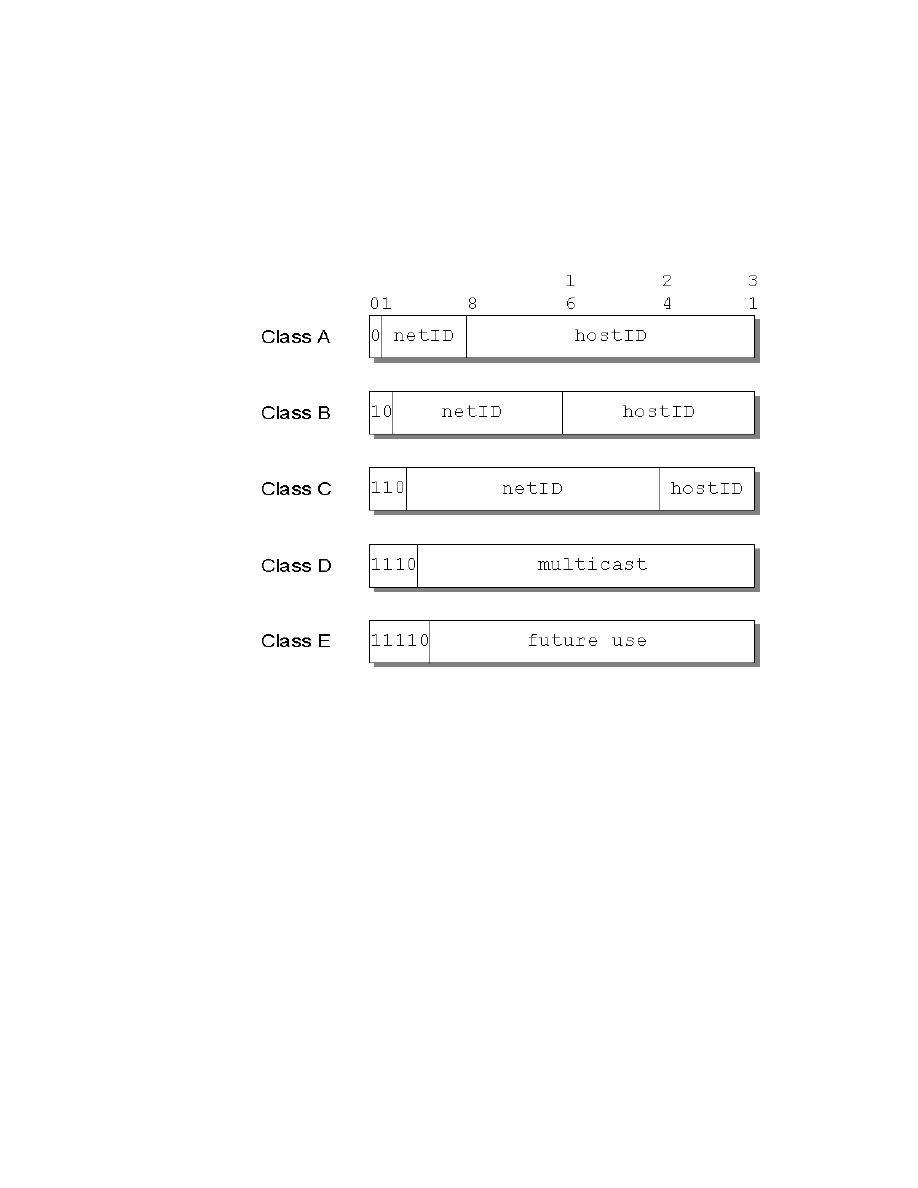
Data Communication
81
represented in the form of four decimal numbers, one decimal number for
each byte (or octet). For example:
00001001 01000011 00100110 00000001
a 32-bit address
9
67
38
1
decimal notation
An IP address consists of two logical parts: a network address and a host
address. An IP address belongs to one of four classes. The class to which
an IP address belongs is determined by the value of its first four bits. See
Figure 18.
Figure 18. Assigned Classes of IP Addresses
• Class A addresses use 7 bits for the <network> and 24 bits for the host
portion of the IP address. That allows for 126 (2**7-2) networks with
16777214 (2**24-2) hosts each; a total of more than 2 billion addresses.
• Class B addresses use 14 bits for the network and 16 bits for the host
portion of the IP address. That allows for 16382 (2**14) networks with
65534 (2**16-2) hosts each; a total of more than 1 billion addresses.

82
Getting Started with Data Warehouse and Business Intelligence
• Class C addresses use 21 bits for the network and 8 bits for the host
portion of the IP address. That allows for 2097150 (2**21) networks with
254 (2**8-2) hosts each; a total of more than half a billion addresses.
• Class D addresses are reserved for multicasting (a sort of broadcasting,
but in a limited area, and only to hosts using the same class D address).
• Class E addresses are reserved for future use.
Some values for these host IDs and network IDs are preassigned and cannot
be used for actual network or host addressing:
• All bits 0
Stands for this: this host (IP address with <host address>=0) or this
network (IP address with <network address>=0). When a host wants to
communicate over a network, but does not know the network IP address, it
may send packets with <network address>=0. Other hosts on the network
interpret the address as meaning this network. Their reply contains the
fully qualified network address, which the sender records for future use.
• All bits 1
Stands for all: all networks or all hosts. For example:
128.2.255.255
Means all hosts on network 128.2 (class B address).
This is called a directed broadcast address because it contains both a
valid <network address> and a broadcast <host address>.
• Loopback
Class A network 127.0.0.0 is defined as the loopback network. Addresses
from that network are assigned to interfaces that process data inside the
local system and never access a physical network (loopback interfaces).
4.1.1.3 Subnets
Because of the explosive growth of the Internet, the principle of assigned IP
addresses became too inflexible to facilitate changes to local network
configurations. Such changes might occur when:
• A new type of physical network is installed at a location.
• Growth of the number of hosts requires splitting the local network into two
or more separate networks.
• Growing distances require splitting a network into smaller networks, with
gateways between them.
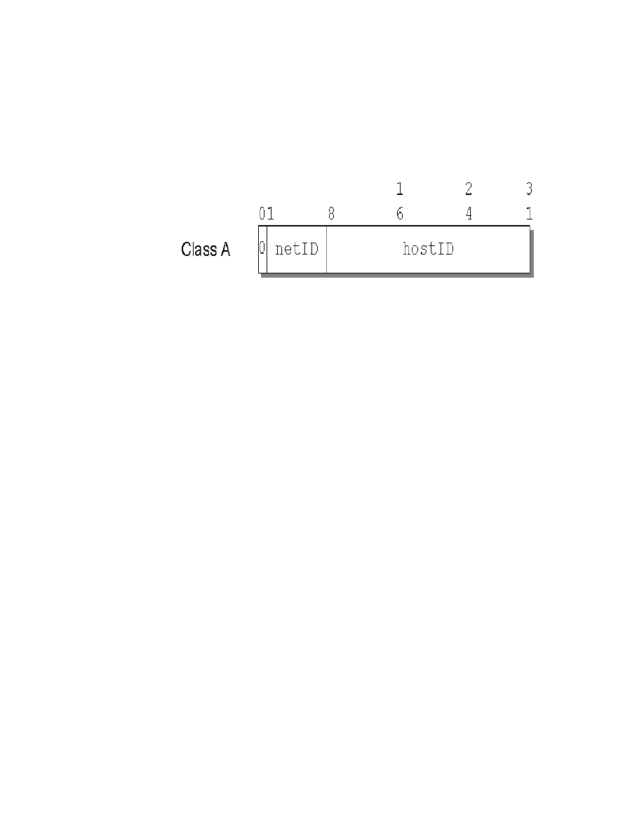
Data Communication
83
To avoid having to request additional IP network addresses in these cases,
the concept of subnets was introduced. The assignment of subnets can be
done locally, as the whole network still appears to be one IP network to the
outside world.
Recall that an IP address consists of a pair <network address> and <host
address>. For example, let us take a class A network; the address format is
shown in Figure 19.
Figure 19. Class A Address without Subnets
Let us use the following IP address:
00001001 01000011 00100110 00000001
a 32-bit address
9
67
38
1
decimal notation (9.67.38.1)
9.67.38.1
is an IP address
(class A)
having
9
as the <network address>
67.38.1
as the <host address>
Subnets are an extension to this by considering a part of the <host address>
to be a subnetwork address. IP addresses are then interpreted as <network
address><subnetwork address><host address>.
We may, for example, want to choose the bits from 8 to 25 of a class A IP
address to indicate the subnet addresses, and the bits from 26 to 31 to
indicate the actual host addresses. Figure 20 shows the subnetted address
that has thus been derived from the original class A address.
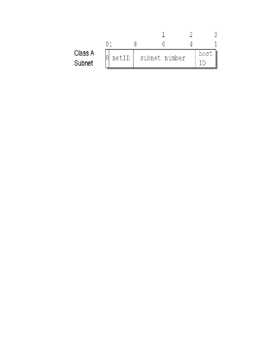
84
Getting Started with Data Warehouse and Business Intelligence
Figure 20. Class A Address with Subnet Mask and Subnet Address
We usually use a bit mask, known as the subnet mask, to identify which bits
of the original host address field to indicate the subnet number. In the above
example, the subnet mask is 255.255.255.192 in decimal notation (or
11111111 11111111 11111111 11000000 in bit notation). Note that, by
convention, the <network address> is masked as well.
For each of these subnet values, only (2**18)-2 addresses (from 1 to 262143)
are valid because of the all bits 0 and all bits 1 number restrictions. This split
will therefore give 262142 subnets, each with a maximum of (2**6)-2 or 62
hosts.
The value applied to the subnet number takes the value of the full byte, with
nonsignificant bits set to zero. For example, the hexadecimal value 01 in this
subnet mask assumes an 8-bit value, 01000000, and gives a subnet value of
64 (and not 1 as it might seem).
Applying this mask to our sample class A address 9.67.38.1 would break the
address down as follows:
00001001 01000011 00100110 00000001 = 9.67.38.1 (class A address)
11111111 11111111 11111111 11------
255.255.255.192 (subnet mask)
=====================================
logical_AND
00001001 01000011 00100110 00------ = 9.67.38
(subnet base address)
and leaves a host address of:
-------- -------- -------- --000001 = 1
(host address)
IP recognizes all host addresses as being on the local network for which the
logical_AND operation described above produces the same result. This is
important for routing IP datagrams in subnet environments (see “IP Routing”
on page 86).

Data Communication
85
The actual number would be:
-------- 01000011 00100110 00------ = 68760
(subnet number)
The subnet number shown above is a relative number, that is, it is the
68760th subnet of network 9 with the given subnet mask. This number bears
no resemblance to the actual IP address that this host has been assigned
(9.67.38.1) and has no meaning in terms of IP routing.
The division of the original <host address> part into <subnet> and <host>
parts can be chosen freely by the local administrator; except that the values
of all zeros and all ones in the <subnet> field are reserved for special
addresses.
4.1.1.4 IP Datagram
The unit of transfer of a data packet in TCP/IP is called an IP datagram.
It is made up of a header containing information for IP and data that is only
relevant to the higher-level protocols. IP can handle fragmentation and
reassembly of IP datagrams. The maximum length of an IP datagram is
65,535 bytes (or octets). There is also a requirement for all TCP/IP hosts to
support IP datagrams of up to 576 bytes without fragmentation.
The IP datagram header is a minimum of 20 bytes long (see Figure 21).
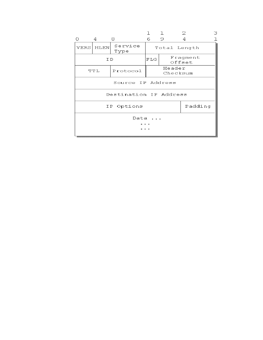
86
Getting Started with Data Warehouse and Business Intelligence
Figure 21. Format of an IP Datagram Header
4.1.1.5 IP Routing
There are two types of IP routing: direct and indirect. For example, Figure 22
shows that the host C has a direct route to hosts B and D, and an indirect
route to host A through gateway B.
Direct Routing
If the destination host is attached to a physical network to which the source
host is also attached, an IP datagram can be sent directly, simply by
encapsulating the IP datagram in the physical network frame. This is called
direct delivery and is referred to as direct routing.
Indirect Routing
Indirect routing occurs when the destination host is not on a network directly
attached to the source host. The only way to reach the destination is through
one or more IP gateways. In TCP/IP terminology, the terms gateway and
router are used interchangeably for a system that actually performs the duties
of a router. The address of the first of these gateways (the first hop) is called
an indirect route in the context of the IP routing algorithm. The address of the
first gateway is the only information needed by the source host.
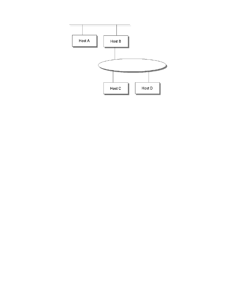
Data Communication
87
Figure 22. Direct and Indirect Routing
IP Routing Table
The determination of available direct routes is derived from the list of local
interfaces available to IP and is composed by IP automatically at initialization.
A list of networks and associated gateways (indirect routes) must be
configured to be used with IP routing if required.
Each host keeps the set of mappings between the:
• Destination IP network addresses
• Routes to next gateways
The mappings are stored in the IP routing table (see Figure 23). Three types
of mappings can be found in this table:
• Direct routes, for locally attached networks
• Indirect routes, for networks reachable through one or more gateways
• Default route, which contains the (direct or indirect) route to be used if the
destination IP network is not found in the mappings of type 1 and 2 above.
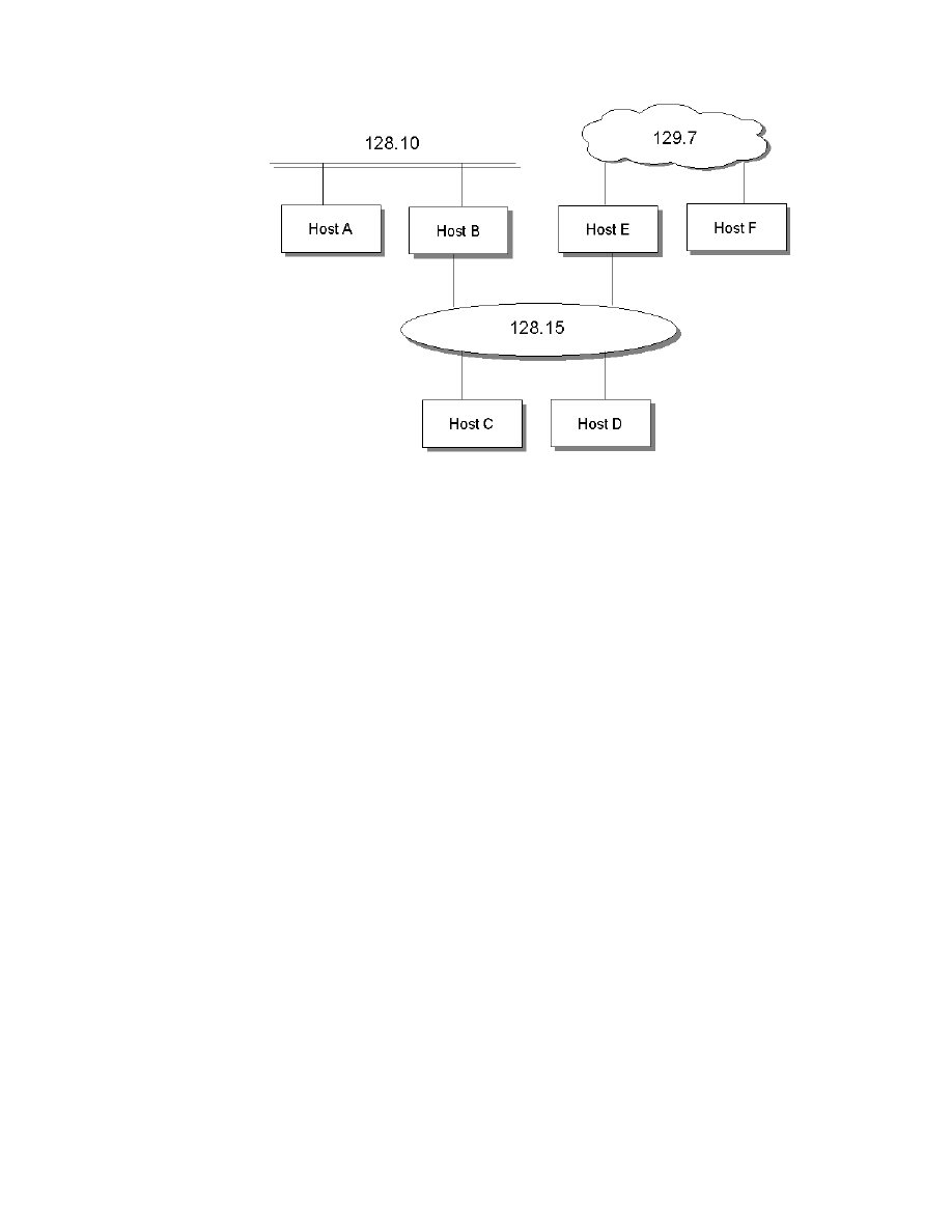
88
Getting Started with Data Warehouse and Business Intelligence
Figure 23. Routing Table Scenario
The routing table of host F might contain the symbolic entries shown in the
Figure 24.
Figure 24. IP Routing Table Entries Example
IP Routing Algorithm
IP uses a unique algorithm to route an IP datagram. Figure 25 shows an IP
routing algorithm with subnets.
destination
router
interface
129.7.0.0
F
lan0
128.15.0.0
E
lan0
128.10.0.0
E
lan0
default
B
lan0
127.0.0.1
loopback
lo
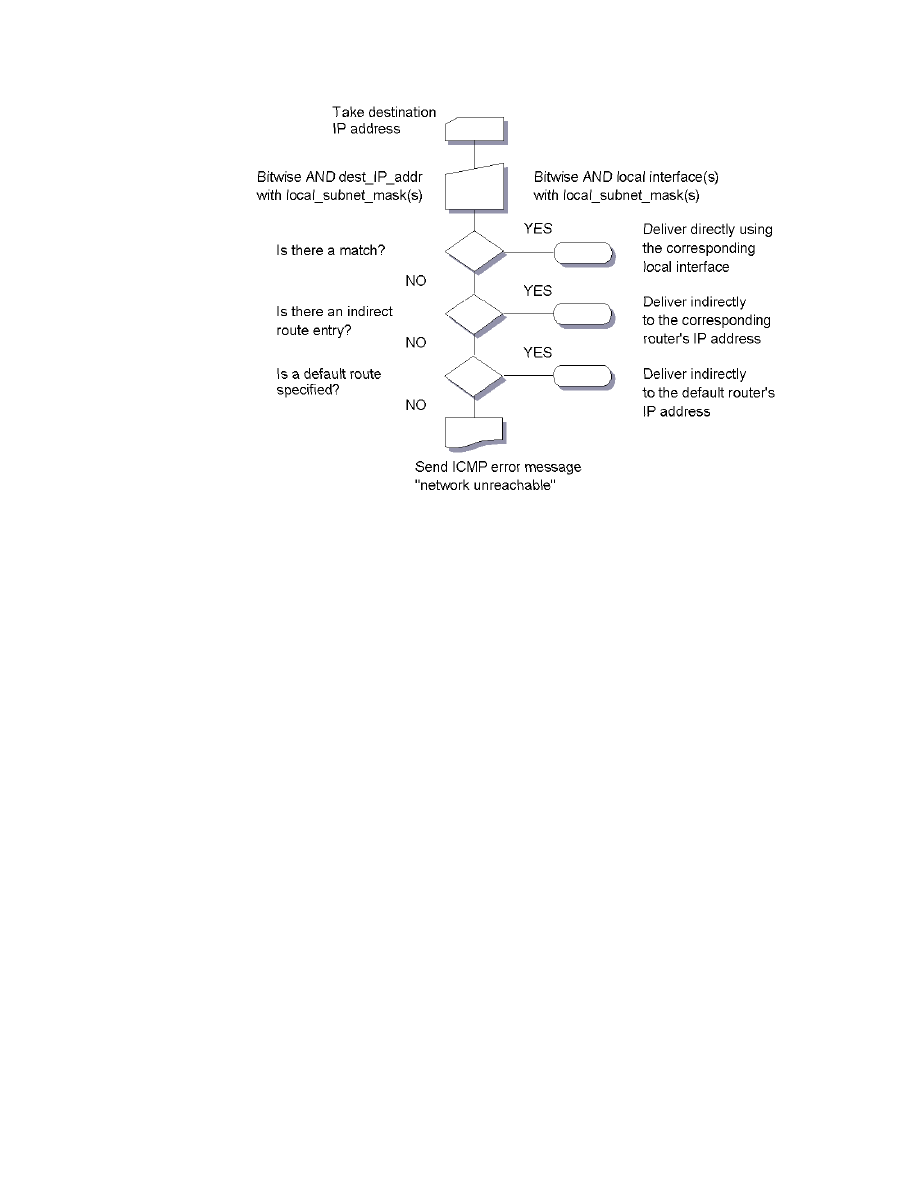
Data Communication
89
Figure 25. IP Routing Algorithm (with Subnets)
Notes:
• IP routing is an iterative process. It is applied by every host handling a
datagram, except for the host to which the datagram is finally delivered.
• Routing tables and the routing algorithm are local to any host in an IP
network. To forward IP datagrams on behalf of other hosts, routers
must exchange their routing table information with other routers in the
network, using special routing protocols.
4.1.2 APPC
The following sections provide information about the advanced
program-to-program communication (APPC) protocol.
4.1.2.1 SNA Basis
SNA is a communications architecture that was originally designed to
address the increasing complexity of data processing and communications
needs as technology advanced. SNA is not a product, it is an architecture
that provides a blueprint or specification of how diverse products can connect

90
Getting Started with Data Warehouse and Business Intelligence
and communicate with each other. It defines a set of rules that describe the
transport of data and specify, for example, what the data looks like, how it is
to be packaged and who the sender and receiver are.
SNA Layers
SNA is a structured architecture that consists of seven well-defined layers,
each of which performs a specific network function. As a result of this
structure, SNA products have compatible interfaces that facilitate
interconnection and communication. Their new functions and technologies
can be added to the network with no disruption to the flow of data. The layers
defined in SNA are:
• Transaction services
Provides application services, such as distributed database access or
distributed file management.
• Presentation services
In general, formats the data for different media and sharing of devices.
• Data flow control
Synchronizes the flow of data within a network, correlates data
exchanges, and groups related data into units.
• Transmission control
Regulates the rate at which data is exchanged to fit within the processing
capacity of the participants to avoid congestion in the transport network.
This layer is also responsible for encryption, if required.
• Path control
Routes data between source and destination and controls data traffic
within the network.
• Data link control
Transmits data between adjacent network nodes.
• Physical control
Connects adjacent nodes physically and electrically and is the hardware
part of the connection.
SNA provides function subsetting at a logical unit (LU) level. Thus the
architecture provides standard option sets, in the form of profiles, which are
defined in the transmission control, data flow control, and presentation
services levels. A specific LU supports a subset of architected profiles that
reduces the number of options specific network products have to implement.
End users (for example, terminal users, applications) access the network

Data Communication
91
through the LU component of a network product. The LU manages the
exchange of data and acts as the intermediary between the end user and the
network.
Network products only need to implement the rules or protocols that support
the type of communication appropriate to the product. Therefore, printers
implement printer protocols, (for example, LU1), and display devices
implement LU2.
With the advent of personal computers, programmable workstations, and
LANs, SNA has led the move toward peer-to-peer networking. Within SNA,
the LU 6.2 protocol is the defined standard for communications between
functionally equivalent LUs. It provides a standard set of formats and
communication rules that allow programs to directly communicate across
multiple hardware and software environments.
4.1.2.2 APPC Basics and Terminology
LU 6.2 describes the standard functions that programs can use to
communicate with each other. The implementation of this protocol is called
APPC. Sometimes LU 6.2 and APPC are used synonymously.
The LU 6.2 Protocol
The LU 6.2 protocol provides a consistent method for programs to:
• Identify and negotiate the communications options to be used by each
partner program
• Provide the name of the partner destination and program
• Supply end-user security parameters to be associated with the request on
the remote platform
• Control the transmission of messages
• Synchronize the processing between the partner programs
• Perform coordinated commit processing
The actual functions that can be used may vary from one APPC
implementation to another. Programs communicate using options that are
supported and agreed to by the APPC support on either side.
Logical Units
The APPC LU implements the LU 6.2 protocol and provides the means by
which transaction programs (TPs) access the network. The SNA software
accepts requests from the TPs, executes them, and routes the data packet
while hiding the physical details of the underlying network. The term local LU

92
Getting Started with Data Warehouse and Business Intelligence
refers to the LU to which a TP issues its APPC calls. The Local LU then
communicates with a partner LU on either the same or a different node.
Transaction Programs
When an APPC application establishes a connection with another LU in the
network, the application must identify the name of the TP it wants to execute.
The TP name is the logical network name that is used by a program to
communicate over the network and can be up to 64 bytes long.
There are two basic types of TPs:
• Application TPs, which perform tasks for end users
• Service TPs, which perform tasks related to system services, such as
changing passwords.
Sessions
The logical connection between LUs is called a session. Sessions are
established when one LU sends another LU the request to BIND. During this
BIND process, both partners exchange information about the characteristics
of the connection to be established. The LU that starts the session, the
initiator, is known as the primary LU, and the recipient of the session is known
as the secondary LU.
LUs have either single-session capability, that is, they allow only one active
LU-to-LU session with a partner LU at a time; or they have parallel-session
capability. With parallel-session support it is possible to have more than one
session with the same partner LU at the same time. Most LUs have
parallel-session capability.
Conversations
To avoid the overhead of session setup every time two LUs want to
communicate, another concept, that of a conversation, has been defined. A
conversation is the logical connection between TPs and is carried out over a
session. Conversations serially reuse a session to exchange end user
information. When a conversation ends, another conversation can be
allocated and use the same session. Sessions are typically long-lived links,
whereas conversations exist for the duration of the exchange of information,
for example, the time it takes to process a transaction.
The basic elements of a conversation are:
• Starting a conversation. When a program wants to start an LU 6.2
conversation with another program, it issues an allocate request. The
ALLOCATE identifies the partner and requests a connection. The APPC
LU makes the connection, if possible, and attempts to reuse a session that

Data Communication
93
was previously established. If none exists, it creates a session. The
partner can accept or reject the conversation request. If the request is
accepted and the conversation established, the caller is put into send
state, the partner is put into receive state, and information can now be
exchanged between the two.
• Exchange of information. The program that is in send state sends
information to its partner, using the SEND_DATA verb. This action causes
the data to be put into the LU's buffer (the LU that is local to the program).
The LU does not actually send the data until either the buffer is full (max
RU for the session on which the conversation is allocated) or the program
explicitly issues a verb (that is, FLUSH, CONFIRM, or one that changes
state) that explicitly causes the LU to transmit the buffered data. The
partner LU accepts the data and buffers it. The TP gets the data and/or
status indicators as a result of issuing a verb such as
RECEIVE_AND_WAIT or RECEIVE_IMMEDIATE.
• Requesting confirmation. TPs can optionally request synchronization of
communications by requesting and granting confirmations, so that they
can determine whether their partners have successfully received data that
they have sent. Requesting confirmation allows programs to agree that
processing completed without error. The level of synchronization (in this
case, CONFIRM) is specified during allocation with the SYNC_LEVEL
parameter. When a TP issues the CONFIRM verb after a SEND_DATA,
the TP actually waits (is suspended) until it receives the response from the
partner. The partner responds that it has either received the data
(CONFIRMED) or that an error has occurred.
• Sending an error notification. When an error occurs, either partner may
inform the other of the condition by issuing a SEND_ERROR or
DEALLOCATE_ABEND.
• Ending conversations. A conversation is ended by issuing a
DEALLOCATE verb. The partner receives both a deallocate indicator and
any remaining data and then may be asked to confirm the deallocation or
just terminate. The partner is put into reset state and completes its own
processing. When a conversation is ended, the session is then available
for use by another conversation.
When TPs communicate over an LU 6.2 conversation, there are a few areas
that they both agree on for compatibility.
Synchronization level provides a means by which two TPs (if they choose to
do so) reach a consistent state of processing with respect to the data
exchanged. The programs on either end synchronize their actions by
requesting and granting confirmations. Confirmation could be used, for

94
Getting Started with Data Warehouse and Business Intelligence
example, when one program wants to ensure that its partner received the
data it sent before deleting the source of the transmitted data. There are
three possible SYNC_LEVELs.
• NONE — specifies no synchronization.
• CONFIRM — allows a TP to request specific acknowledgment from a
partner that it has received a message. This SYNC_LEVEL enforces
confirmation exchanges and error reporting. There are two flavors of
confirmation. The first is one wherein a TP issues a CONFIRM verb, to
which the partner replies either positively with CONFIRMED, or reports an
error condition with SEND_ERROR. The second one is where a TP
requests confirmation from its partner by issuing a verb such as
DEALLOCATE with type=SYNC_LEVEL.
• SYNCPOINT — allows all transaction programs in a distributed
environment to commit or back out changes to protected resources (that
is, databases). The LU takes responsibility for syncpoint processing.
A synchronous conversation is characterized by a transaction program
issuing an ALLOCATE of a conversation, a SEND of data, and a RECEIVE for
the reply. When the partner detects that the input message is complete, that
is, the partner program enters the RECEIVE state, the conversation is
considered to be synchronous. Replies are sent back on the same
conversation.
An asynchronous conversation is characterized by a transaction program
issuing an ALLOCATE of a conversation, a SEND of data, and a
DEALLOCATE. This conversation allows the originating TP to do other work
while the partner processes the request. The conversation is in RESET state.
If an output reply is to be sent back, a new conversation to send the reply is
allocated.
The choice of a MAPPED or BASIC conversation type affects the format of
data transmission. An APPC logical record is a sequence of length "LL"
(2 bytes) and "data" fields. A typical pattern is "LLdataLLdata..." where the LL
fields define how much data follows before the next length field. The choices
for preparing the data for transmission in this manner are:
• MAPPED — Lets APPC format the data into and out of this pattern for
each transmission. The handling of the details of the underlying data
stream is the responsibility of the APPC LU and not the application. Thus
applications are easier to code because they only need to prepare the
data in the format that the partner expects.

Data Communication
95
• BASIC — Requires the TPs to be responsible for formatting the data and
including the LL field. This puts the burden on the TP rather than the
APPC LU.
Common Programming Interface for Communications
Because the LU 6.2 architecture provides freedom of syntax, products such
as APPC/MVS, OS/400, and OS/2 have the option of creating unique
implementations of the APPC API as long as they adhere to the semantics
(services) as defined by the architecture. As a result of this freedom, the
different products have in fact done so. This makes it very complicated for
APPC programmers who have to program in different environments, because
they are faced with having to learn the unique API appropriate to an
implementation. For example, to issue an allocate verb in the APPC/MVS
environment, a programmer codes ATBALLC; in an OS/2 environment, a
programmer would use the MC_ALLOCATE verb, and in an OS/400
environment, a programmer would use the ACQUIRE and EVOKE verbs.
To alleviate this problem, a standard and consistent API has been defined for
applications that need to communicate in the APPC arena. The Common
Programming Interface for Communications (CPIC) is common across
multiple environments and differs from the product-specific APIs in that it
provides an exact common syntax to specify the function calls and
parameters. CPIC is designed to eliminate the mismatch of the verb
specifications in the different environments. This capability allows an
application programmer to learn the syntax on one platform and port the
knowledge or even part of the program to another supporting platform.
Application programs can use CPIC calls in the major languages such as
COBOL, C, FORTRAN, and PL/I. Pseudonym files are provided in the
different operating environments (in MVS, check SYS1.SAMPLIB). The files
can be "included" or "copied" into programs that call CPIC.
It is up to an application programmer to decide whether to use CPIC or the
native interface unique to the specific APPC implementation.
Advanced Program to Program Communication (APPC) is the System
Network Architecture (SNA) protocol, on which Distributed Relational Data
Architecture (DRDA) is based. APPC is used for the communication between
the host system and the workstation servers. The necessary definitions for
the APPC protocol are much easier to handle using VTAM/Advanced Peer to
Peer Networking (APPN) on the host side. That means some of the
definitions are made automatically during startup of communication.
For the time being, TCP/IP is not supported by DB2 for VSE V5, one of the
host data servers for this project, just having support for APPC protocol.

96
Getting Started with Data Warehouse and Business Intelligence
To set up DRDA in VM, we need APPC/VM VTAM Support (AVS), which
handles the communications between VM and non-VM systems in the
network. DB2 communicates by using Inter User Communication Vehicle
(IUCV) with the AVS virtual machine. Coordinated Resource Recovery (CRR)
provides the synchronization services for two-phase commit processing. A
VM CMS application can act as a DRDA client to access any DRDA server.
On VSE, CICS handles the DRDA connectivity and also supports the
two-phase commit processing. VSE itself uses Cross Partition
Communication (XPCC) to talk to CICS.
APPC communication can be used for communication with CrossAccess
Servers as well. CrossAccess is able to work as a VTAM application, not
requiring use of the CICS. This allows the possibility of using native TCP/IP
for VSE with this products. Details about this configuration will be described
later in this book.
4.2 Data Exchange Protocols
This heading discusses the different options and capabilities for accessing
and transferring data between different systems. More detailed information
about the following headings can be found in From Multiplatform Operational
Data to Data Warehousing and Business Intelligence, SG24-5174.
4.2.1 DRDA Remote Unit of Work (RUW)
The remote unit of work, also referred to as DRDA level 1, offers remote data
access from an Application Requester (AR) to an Application Server (AS).
RUW means one Database Management Subsystem (DBMS) is accessed
with one logical unit of work. After changed data has been committed, the
application might switch to another DBMS, even on another platform.
The AR functionality is available not only on the workstation side. An
application running on OS/390 or VM might access a workstation DBMS as
well. The way to define the remote access is different on the different
platforms. On OS/390 all definitions are held in DB2 tables, whereas the VM
side requires some definitions on the operating system side as well. The PC
systems (Windows and OS/2) offer a GUI for all required definitions.
4.2.2 DRDA Distributed Unit of Work (DUW)
The distributed unit of work represents the DRDA level 2, giving access to
more than one DBMS within one logical unit of work. That is, the application

Data Communication
97
might switch to another DBMS before committing the data on all sites in
parallel. A funds transfer from one DBMS to another is the best sample for
such an application. If the update on one side fails, the changes on the other
side are rolled back as well. So there is no risk of an inconsistency in
between. The DUW requires a Two Phase Commit functionality on all
participating DBMSs.
4.2.3 Distributed Request (DR)
The two phase commit function is the base for the distributed request as well.
DR means access to several DBMS within one select statement. With this
functionality, a join of data from multiple systems is possible. The IBM
DataJoiner (DJ) offers this function when providing several (remote) data
sources as one single database image. The SELECT SQL statement (join of
two or more tables) is issued against the DJ database, and the middleware
splits it up to several DUW requests or transfers the data and performs the
join locally.
4.2.4 Private Protocols
Private protocols are used within the DB2 family for communication between
the Universal Database (UDB) products on the workstation side. This private
protocol provides same functionality as DRDA.
The SQLDS private protocol is used for communication between DB2 Server
for VM and DB2 Server for VSE through Guest Sharing only. It provides no
DRDA functionality. With the setting of the DB2 for VSE or VM start-up
parameter ’PROTOCOL’ to either ’AUTO’ or ’SQLDS’, you may decided
whether the database server accepts a DRDA request or private protocol
only. See the ’Operation’ or ’System Administration’ manual for more details.
4.2.5 Nonrelational Access
For the access to nonrelational data from a "relational" requester, there are
no specific protocols to be named; only products.
OS/390
A feature of DataJoiner called Classic Connect provides access to IMS and
VSAM data on OS/390 in a relational view. A server application running on
the host, maps the nonrelational data to the specified table image using meta
data. This meta data is generated from the COBOL copy books or the
database descriptor block (DBD for IMS), which describe the format of the
data records.

98
Getting Started with Data Warehouse and Business Intelligence
VSE/ESA
A similar function is provided for access to VSAM, DL/I, and sequential files
on VSE by CrossAccess. The Server is running permanently on the host to be
accessed either through TCP/IP or APPC. For every request, a Database
Management System Interface (DMSI) is started in another (dynamic)
partition. The DMSI accesses the nonrelational data, while the server maps it
to the relational table image by using the meta data, as described for Classic
Connect.
So far, the access to the nonrelational data is read-only. Joining of tables is
possible for "like" data; that means, for example, two VSAM tables.

© Copyright IBM Corp. 1999
99
Chapter 5. Implementation
This chapter describes how the host servers were implemented in the ITSO
scenario, providing samples that can help you in your implementation.
5.1 OS/390 Environment
This section explains how to configure the environment to access IMS
databases, VSAM files, and DB2 databases under the OS/390 environment
from a client workstation through the DataJoiner and DataJoiner Classic
Connect products.
The following steps are required to configure this environment under the
OS/390 by using the DataJoiner and DataJoiner Classic Connect.
1. Section 5.1.1, “IMS/ESA Environment Configuration” on page 99, shows
you how to configure the IMS Database control (DBCTL) environment if
you use the database resource adapter (DRA).
2. Section 5.1.2, “DataJoiner Classic Connect Configuration” on page 100,
shows you how to configure DataJoiner Classic Connect.
3. Section 5.1.8, “DataJoiner Connectivity” on page 123, shows you how to
configure DataJoiner.
See Appendix A, “The OS/390 Environment” on page 177, for detailed
information about how all the source databases were created for this project,
on the OS/390 system.
5.1.1 IMS/ESA Environment Configuration
This section describes how to prepare the IMS/ESA environment to access
the IMS Database from the DataJoiner through the DataJoiner Classic
Connect (DJCC). The following paragraph gives a short introduction to the
IMS system.
IMS consists of two licensed programs: the IMS Database Manager (DM) and
the IMS Transaction Manager (TM). With the Database Manager, you can
generate the batch environment and the database control (DBCTL)
environment. With both the Database Manager and the Transaction Manager,
you can generate the DB/DC environment. With the Transaction Manager,
you can generate the data communication control (DCCTL) environment.
The greatest dissimilarity between DBCTL and DB/DC is that DB/DC is a
complete on-line transaction and database management system. DBCTL is a

100
Getting Started with Data Warehouse and Business Intelligence
database management system only. No communication facility, such as
VTAM or TCP/IP, is available on DBCTL. Also, DBCTL supports part of the
Fast Path database. No IMS remote site recovery and share queue address
spaces exist. The Batch Message Processing (BMP) region is used only by
batch applications and utilities. External program subsystems can, however,
use an interface that does handle messages—a coordinator controller
(CCTL). The interface between the CCTL and the control region is the
database resource adapter (DRA).
The DRA is provided by IMS, but does not reside in any IMS on-line or
associated address spaces. Instead, it resides in "client" address space.
For example, when CICS connects to DBCTL, DRA resides in CICS address
space, and communicates with DBCTL’s partition support table (PST) control
block.
The DJCC allows you to access IMS data using either its DRA interface or its
BMP/DB Batch (DBB) interface. The DJCC is a VTAM application; it uses IMS
CCTL modules, but resides in DJCC address space, not in IMS.
Using the DRA interface, you must use the IMS DBCTL control region, you
must configure the DRA interface in your DJCC data server configuration file,
and you must start the DJCC data server using the DRA interface
parameters. If you have to configure the IMS DBCTL control region in your
IMS environment, as we did for this project, see Appendix A, “The OS/390
Environment” on page 177, for help in configuring it.
Using the BMP/DBB interface, you can use the IMS control region from either
DBCTL or DB/DC. You must configure the BMP/DBB interface in your DJCC
data server configuration file, and you start the DJCC data server using the
BMP/DBB interface parameters.
We describe how to configure the DJCC data server under “Establish
Connectivity between IMS and DJ through DJCC” on page 123 in this
redbook.
For more detail information about configuring IMS DBCTL, see the manual
IMS/ESA V6 Admin Guide: System, SC26-8730.
5.1.2 DataJoiner Classic Connect Configuration
This section describes how to configure the DJCC configuration files.

Implementation
101
5.1.2.1 Data Server Installation Verification
After you have finished the installation, and before you continue with the
configuration, we strongly recommend that you go through the installation
verification program.
The OS/390 Sample Application (DJXIVP) is available in the installation IVP
sample library (djxhlq.DJXSAMP). Make sure that this JOB correctly
generates the same output as the sample output (DSXIVOUT) in
djxhlq.DJXSAMP. The return code is 0, even if the queries from the sample
application failed. You have to check the output file carefully.
5.1.2.2 Data Server Setup for IMS Access
This section describes the Data Server setup for IMS Access by the DRA
interface. You do not need this setup for the BMP/DBB interface.
A coordinator controller (CCTL) provides communications and transaction
management services for a DBCTL environment, which has no transaction
management facilities of its own.
1. Make DFSPRRC0 accessible:
The Classic Connect uses the CCTL. The CCTL must load the DRA
start-up/router (load module DFSPRRC0). Although the DRA is shipped
with the IMS product, it executes in the CCTL address space, that is the
Classic Connect data server.
Make the DFSPRRC0 accessible to the Classic Connect data server using
either of the following methods:
• Copy DFSPRRC0 from the imshlq.RESLIB library into the
djxhlq.SDJXLOAD load library.
• Concatenate the imshlq.RESLIB library to the SDJXLOAD STEPLIB.
2. Create DFSPZPxx:
The DRA start-up table (load module DFSPZPxx) contains default values
for the DRA initialization parameters. If the system programmer wants to
specify values other than the defaults, write your own module (naming it
DFSPZPxx), assemble it, and load it in the CCTL load library. Use the
supplied module, DFSPZP00, as an example. See the following example:

102
Getting Started with Data Warehouse and Business Intelligence
EJECT
DFSPRP DSECT=NO,
X
FUNCLV=1,
X
CCTL FUNCTION LEVEL
X
DDNAME=CCTLDD,
XXXXXXXX DDN FOR CCTL RESLIB DYNALOC X
DSNAME=IMS610D.RESLIB,
X
DBCTLID=IMSD
,
NAME OF DBCTL REGION
X
USERID=YOURID,
XXXXXXXX NAME OF USER REGION
X
MINTHRD=001,
XXX
MINIMUM THREADS
X
MAXTHRD=005,
XXX
MAXIMUM THREADS
X
TIMER=60,
XX
IDENTIFY TIMER VALUE - SECS X
SOD=T,
X
SNAP DUMP CLASS
X
TIMEOUT=060
XXX
DRATERM TIMEOUT IN SECONDS
END
Set "DSECT=NO".
Set "DSNAME" to imshlq.RESLIB. In our example,
"DSNAME=IMS610D.RESLIB".
Set "DBCTLID" to your IMS subsystem id. In our example,
"DBCTLID=IMSD".
Make the load module DFSPZPxx accessible to the Classic Connect data
server. In our example, "SJ" is used for the suffix, and it is stored into
IMS610D.RESLIB and is specified in STEPLIB of the data server started
JCL.
The SERVICE INFO ENTRY parameter for DRA specifies the suffix xx for
the start-up tables name. You specify it in Data Server Configuration file.
An example follows:
*
* IMS DRA INTERFACE SERVICE INFO ENTRY
*
REFER TO CLASSIC CONNECT DOCUMENTATION FOR DETAILED
*
INFORMATION ON LAST SUBPARAMETER
SERVICE INFO ENTRY = DJXDRA IMS
2 1 1 10 4 5M 5M SJ,YOURDID,PFIRDB
5.1.3 Network Communication Protocol Configurations
This section describes the steps you must perform, both on your OS/390
system and on your AIX system, to configure a TCP/IP communications
interface (CI) for DJCC.
5.1.3.1 Configuring TCP/IP on OS/390
DJCC’s TCP/IP is compatible with both IBM’s and Interlink’s Berkeley Socket
TCP/IP. This section describes how to configure Classic Connect using IBM’s
TCP/IP.

Implementation
103
Berkeley sockets is supported by IBM and Interlink. The Berkeley Sockets
version requires an additional parameter in the DJXDSCF member called
TASK PARAMETER, which identifies the Interlink subsystem name and
identifies the location of the configuration data sets for IBM. Within the
configuration data sets, users must specify the name of the started-task
procedure used to start the TCP/IP address space name and can also specify
the TCP/IP DNS IP addresses. If no environment variables are passed, then
the default value TCP/IP is used for both the address space name and as the
high-level qualifier (hlq) of the standard configuration files:
• hlq.TCPIP.DATA
• hlq.ETC.HOSTS
• hlq.ETC.PROTOCOLS
• hlq.ETC.SERVICES
• hlq.ETC.RESOLV.CONF
DJCC uses a search order to locate the data sets, regardless of whether
DJCC sets the hlq or not.
Determine the following values for the OS/390 system on which DJCC is
being installed, and enter these values in the worksheet portion of Figure 26:
• IP Address (or hostname)
is specified in the hlq.PROFILE file under the parameter of HOME.
• Port Number (or service name)
is not specified in the hlq.PROFILE file under PORT parameters for
another application.
• TCP/IP address space name
is specified in subparameter TCPIP_MACH of TASK PARAMETER, which
must be the same name in the hlq.TCPIP.DATA file under the parameter of
TCPIPJOBNAME.
• High level qualifier of TCP/IP standard configuration files
is specified in subparameter TCPIP_PREFIX of TASK PARAMETER.
5.1.3.2 Configuring TCP/IP on AIX
You must configure your AIX machine to locate the DJCC data server on
OS/390.
1. Update the Names server or /etc/hosts file on the AIX machine with the
hostname value. If you are using an IP address, no action is required.

104
Getting Started with Data Warehouse and Business Intelligence
2. On the AIX machine, you can configure either a port number or service
name to access a particular data server. If you are using a service name, it
must be defined in the /etc/services file on the AIX machine. If you are
using a port number, no action is required.
5.1.3.3 TCP/IP Communications Template and Worksheet
Figure 26 provides you with an example set of TCP/IP values for both your
OS/390 configuration. The values will be used during DJCC Data Server and
client configuration in a later step.
Figure 26. TCP/IP Communications Template and Worksheet
5.1.4 Configuring Data Server Communications on OS/390
DJCC data server can accept communication connections from both local
and remote client applications.
Three parameters are involved in configuring a client application to DJCC
data server connection:
• The DATASOURCE parameter in the client
The client’s DATASOURCE parameter specifies two subparameters:
• The data source name
• A communications compound address field
• A SERVICE INFO ENTRY parameter in the data server for a query
processor (DJXQP)
• A SERVICE INFO ENTRY parameter in the data server for a connection
handler service (DJXINIT)
Figure 27 shows the relationship of the DJCC configuration files and other
related parameters.
TCP/IP-MVS
MVS hostname
not used (*)
or IP address
9.12.14.223
subsystem name
tcp
port number or service
3500
name for data server
(*)This example uses IP address instead of the hostname
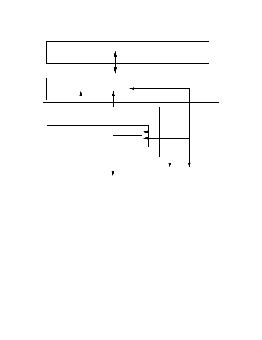
Implementation
105
Figure 27. Relationship of DJCC Parameters
DJX_CC2-config=/data/djinst2/sqllib/djxclassic2.cfg
export DJX_CC2_CONFIG
DataJoiner Instance on AIX
DB2PROFILE
DJCC Configuration file(djxclassic2.cfg)
DEFLOC=DJXSAMP
DATASOURCE=MVSCC tcp/9.12.14.223/3500
MVS IP address
Data Server port number
DataJoiner Classic Connect for OS/390
TCP/IP OS/390
Data Server Master Configuration file OS/390
SERVICE INFO ENTRY = DJXINIT TCPIP 2 1 1 100 4 5M 5M TCP/ 9.12.14.223/3500
SERVICE INFO ENTRY = DJXQP MVSCC 2 0 2 50 4 5M 5M DJXQPCF
TASK PARAMETERS == TCPIP__PREFIX=TCPIPMVS.SC53=TCPIP__MACH=TCPIPMVS
9.12.14.223
3500

106
Getting Started with Data Warehouse and Business Intelligence
5.1.5 Configuring an AIX Classic Connect Client
The following steps describe how to configure a DJCC instance to access a
DJCC data server.
1. Edit the DJCC configuration file, djxclassic2.cfg.
The configuration file, djxclassic2.cfg, shown in Figure 28, is located in the
DataJoiner instance owner’s sqllib directory; for example,
/home/djinst/sqllib/djxclassic2.cfg. Each instance has its own configuration
file.
Figure 28. Example of Classic Connect Configuration file, djxclassic2.cfg
2. Configure DATASOURCE parameter for TCP/IP.
Modify the DJXSAMP DATASOURCE parameter to include the IP address
(or hostname) and port number (or service name) of the data server.
While configuring the data server in “Configuring Data Server
Communications on OS/390” on page 104, you may have added
additional query processor SERVIVE INFO ENTRYs. Add DATASOURCE
statements for any additional query processors to be accessed using
TCP/IP.
The sample configuration file contains an entry for the SFVTAM query
processor. If you are not using APPC to configure a data server, comment
this DATASOURCE statement out by adding an asterisk (*) as the first
character of the line.
3. Uncomment the DEFLOC configuration parameter.
4. Save the file to disk.
***********************************************************************
*
Classic Connect Sample Application Configuration File
*
***********************************************************************/
* national language for messages
NL
= US English
* resource file master file
NL CAT = /data/djinst2/sqllib/msg/En_US/djxengcat2
FETCH BUFFER SIZE = 32000
DECODE BUFFER SIZE = 4096
DEFLOC = MVSCC
USERID = yourid
USERPASSWORD = password
DATASOURCE = MVSCC tcp/9.12.14.223/3500
*DATASOURCE = SFVTAM appc/sideprofile1/remote1tpname
HOST CODEPAGE = IBM-850
NETWORK CODEPAGE = IBM-037
RESPONSE TIME OUT = 20S
COMPRESSION = 0

Implementation
107
5. Set environment variables.
The DJX_CC2_CONFIG environment variable must be set to point to the
DJCC configuration file on AIX, djxclassic2.cfg. For example:
export DJX_CC2_CONFIG=/home/djinst2/sqllib/djxclassic2.cfg
This variable must be set for each DataJoiner instance or user running
DJXSAMP2 to access DJCC. Set DJX_CC2_CONFIG from your AIX
command prompt, from the shell initialization file (see Figure 29), or from
the instance profile scripts (see Figure 30).
Figure 29. Example of .profile
Figure 30. Example of db2profile
Access from DataJoiner will be available only after the instance is restarted
using the DB2 start command.
5.1.6 Mapping Non-Relational Data (VSAM)
5.1.6.1 Data Mapper
This section explains how to use the Data Mapper.
export LIBPATH=\home\djinst2\sqllib\bin;
export DJX_CC2_CONFIG=\home\djinst2\sqllib\djxclassic2.cfg
:
#-----------------------------------------------------------------------
# DJX_CC2_CONFIG [Default= null, Value: name of the CC V2.1.1 config file]
# specifies the complete path and file name of the configuration file
# for the DataJoiner Classic Connect (CC)V2.1.1 interface.
If set
# and the file exists, support for the CC is enabled.
If null, not
# set, or DataJoiner cannot find the file, the CC interface cannot be
# used.
The CC interface is used to access data sources defined to
# DataJoiner Classic Connect V2.1.1 for MVS.
A sample setting is:
#
DJX_CC2_CONFIG=/data/djinst2/sqllib/djxclassic2.cfg
#-----------------------------------------------------------------------
DJX_CC2_CONFIG=/data/djinst2/sqllib/djxclassic2.cfg
export DJX_CC2_CONFIG
:

108
Getting Started with Data Warehouse and Business Intelligence
Creating a Repository
The first step in mapping your non-relational data to a relational view is to
create a repository.
A repository stores information (data catalogs, tables, columns, and owners)
about the legacy data DataMapper is mapping.
To create a repository:
1. Select File -> New Repository from the DataMapper main menu.
2. Enter a File Name and location for your repository in the Create a New
Repository dialog box. A file extension of .mdb must be assigned to all
DataMapper repository files.
3. Click Save to create the repository. The repository you created is
displayed. This is an empty repository. You will add data catalogs to the
repository in “Creating a Data Catalog” on page 108.
Creating a Data Catalog
This step describes how to create a data catalog for the newly-created
repository.
1. With the repository window open, select Edit -> Create a New Data
Catalog... from the DataMapper main menu, or click the Create a New
Data Catalog icon on the toolbar.
The Create Data Catalog dialog box opens.
2. Enter the data catalog Name, Type, and any Remarks. To select from a
list of data catalog types, click the arrow next to the Types box.
3. Click OK to create the data catalog.
The data catalog is now displayed on your repository screen.
Creating a Table
The following steps describe how to add tables to a data catalog.
A Classic Connect table is equivalent to a DB2 table and is created by
mapping one or more record types from a non-relational database into a
single Classic Connect table.
Be sure to have a repository open before starting this section.
1. Select a data catalog by clicking the number to the left of the data catalog
name. This will highlight the selected row.
2. Double-click the Table icon to bring up the Tables window, or select
Window -> List Tables to list tables for the data catalog.

Implementation
109
3. From the Tables window, select Edit -> Create a new table..., or click the
Create a New Table icon on the toolbar.
The Create a VSAM Table window opens.
4. Enter the table Name in the Name box.
5. Choose an Owner from the pulldown list.
6. Enter the data set name or the DDname of the data set for a VSAM DMSI:
• For a data set name, select the DS radio button. Enter a 1- to
44-character MVS data set name, such as SYS1.VSAMKSDS, in the
Name field.
The DS option users MVS dynamic allocation services to access the
associated VSAM data set.
• For a DD name, select the DD radio button. Enter a 1- to 8-character
alphanumeric DDname in the Name field.
The DD option requires a DD statement with that DDname in the VSAM
DMSI start-up procedure JCL.
7. (Optional) Select Reference Only by clicking the box to the left of the
Reference Only field.
This selection specifies that the table you are creating will be used for
reference purposes only. The reference table is used to build large column
lists to populate other tables. These reference tables are not generated
into the data catalog’s meta data input when meta data generation is
requested. This option is particularly useful when creating tables with
hundreds of columns, as you can use the drag-and-drop feature of
DataMapper to copy columns between windows.
8. Enter any remarks in the Remarks box.
9. Press Enter, and the table is added to the data catalog.
10.Click OK to create the table.
The table is added to the VSAM Tables for Data Catalog window for this
data catalog.
Importing a Copybook
This section describes how to import a COBOL copybook. Copybooks are
transferred from the mainframe to the workstation and must be given a file
extension of .fd.
1. Open the VSAM Tables for Data Catalog window by double-clicking the
Table icon, or selecting Window -> List Tables.

110
Getting Started with Data Warehouse and Business Intelligence
2. Select the table into which you want to import the copybook by clicking the
number to the left of the table name.
3. Select File -> Import External File..., or press the Import an External
File icon.
The Import File dialog box opens.
4. Select a copybook to import from the C:\cxa32\dm\samples directory and
then click Open.
The Import Copybook window opens.
5. Select the table into which you which you want to import the copybook,
and select the appropriate import options, which include:
Import Group Level Data Items
Creates a column for each COBOL data item that is a group level item.
Group level items are items without picture clauses that contain
subordinate data items with higher level numbers.
Import Selected Structure Only
Since most copybooks contain more than one record or field definition,
you can select a particular structure to import from an existing
copybook by clicking on the data item at which to start the import, then
selecting the Import Selected Structure Only check box. When
structure selection is used, the selected data item and all subordinate
data items (following data items with higher level numbers) are
imported. The data item selected can exist at any level in the structure.
OCCURS Clauses
• Create Record Array: defines a record array for data items within
OCCURS clauses in the copybook.
• Expand each occurrence: creates a column for each occurrence of a
data item within the copybook. Data item names within the OCCURS
clause are suffixed with _1, _2, ..._n.
• Map first occurrence only: create a column for the first occurrence of
a data item within the OCCURS clause only.
Append to Existing Columns
Adds the copybook columns to the bottom of the list of existing columns in
that table. Not selecting this option deletes any existing columns and
replaces them with the columns you are now importing.

Implementation
111
Calculate Starting Offset
Use this option to append to existing columns in a table. This allows the
starting offset of the first appended column to be calculated based on the
columns already defined in the table. When selected, the first appended
column will be positioned at the first character position after the last
column (based on offset and length already defined for the table).
Use Offset
When you have an explicit offset to be used for the first column imported
and it does not match the field’s offset in the copybook structure, enter an
offset in this field to override the default calculation based on the COBOL
structure. If you do not override the default, the offset for the first imported
column is determined by the COBOL field’s offset in the structure you are
importing.
Note: By default, the offset of the first COBOL data item imported is based
on the data item’s position in all of the structures defined in the import file.
This offset will always be zero unless you are importing a selected
structure from the copybook. In that case, the offset for the first column
imported from the structure will be the COBOL data item’s position based
on all structures that precede it in the import file. If the default offset is not
correct, then the Calculate Starting Offset or Use Offset options can be
used to override the default.
6. Select Import to import the copybook to your table.
The Columns for VSAM Table window opens with the newly-imported
columns.
Creating VSAM Index
Note: Be sure to have the VSAM Tables window open and a table selected
before starting this section.
1. Select Window -> List Indexes, or click the Index icon on the toolbar to
list the indexes of the table.
2. Select Edit -> Create a new Index..., or select the Create a New Index
icon on the toolbar.
The Create VSAM Index window opens.
3. Enter the following information:
Name
Specifies the name of the index (required).
Owner
Specifies the authorization ID to be assigned to the index (optional).

112
Getting Started with Data Warehouse and Business Intelligence
Index is Unique
If checked, every key in the index has a unique value.
VSAM Alternate Index
Select either DD or DS and enter 1- to 8-character DD Name or 1- to
44-character VSAM PATH name (optional).
If alternate index information is not defined, the index is assumed to be
the primary index of a VSAM KSDS.
Included Columns
Contains the columns comprising the index and their physical order in
the index. At least one column must be defined in the included columns
list.
Remarks
Description of the VSAM index (optional).
4. Click OK to add the index.
The Indexes for VSAM Table window opens with your new index added.
Generate VSAM Meta Data Grammar
This section describes the steps required to create meta data grammar. Meta
data grammar, also known as USE grammar, is generated by the DataMapper
for all of the tables in a specific data catalog. When meta data grammar has
been created, it is subsequently transferred from the workstation to the
mainframe. It is required as input to the Classic Connect Meta data Utilities
that are run on the mainframe to create tables and used as
relational-equivalent data maps for their corresponding non-relational files.
1. From the Data Catalog window, select a data catalog.
2. Select Generate USE Statements... from the File menu or select the
Generate USE icon on the toolbar.
The Generate USE Statements window opens.
3. Give the file a name, using .use as the file extension, for example,
generate.use.
4. If you click Yes, the following screen appears asking if you want to view
the newly-created script.
Click Yes, and the USE statement script displays.
Note: If you define duplicate table names, the DROP table statement
deletes the old table and creates the new table with the newly-generated
USE statement.

Implementation
113
If necessary, you can edit this file directly from the notepad where it
appears.
5.1.6.2 Meta Data Utility
The meta data utility is used to complete the process of mapping
nonrelational data into a relational logical table that Classic Connect is
capable of accessing. The meta data utility accepts meta data grammar as
input, which contains the nonrelational-to-relational mapping information. The
meta data utility reads the meta data grammar and populates meta data
catalogs for use by the Query Processor. The meta data catalogs are stored
in two files referenced by the DJXCAT and DJXINDX DD statements in both
the meta data utility, and the Data Server JCL streams. The meta data utility
supports incremental updates to the meta data catalogs, and can be run
while data servers are active.
1. Edit the meta data utility JCL.
Sample meta data utility JCL is found in SDJXSAMP member METAUTL.
The contents of the METAUTL member are shown in A.4.4.3, “Meta Data
Utility” on page 221.
Sample meta data utility JCL is found in SDJXSAMP member METAUTL.
The contents of the METAUTL member is shown in A.4.4.3, “Meta Data
Utility” on page 221.
2. Basic Customization.
Supply a valid jobcard and modify the DJX high-level qualifier to reference
the high-level qualifier for the Classic Connect-supplied data sets. At this
point you may want to save the member, since the DJX high-level qualifier
is not likely to change from run-to-run of the meta data utility.
3. Customize VSAM mappings.
When mapping VSAM data, the meta data grammar can reference the
VSAM file to be accessed by the logical table, either by its data set name
or using a DD name. When referenced by a data set name, the meta data
utility dynamically allocates the data set name referenced, by checking for
its existence and gathering physical attributes about the file.
If you are referencing a file by DD name, then you need to add DD
statements with the same DD names in the meta data utility JCL. You
should specify a DISP=SHR for these data sets. The meta data utility will
open these files during processing in order to obtain physical information
about the files.

114
Getting Started with Data Warehouse and Business Intelligence
4. Determine whether you need to create the meta data catalogs.
The first time you run the meta data utility, you must create the meta data
catalog files. For the installation verification process, you must create a
new set of meta data catalogs.
To create a new set of meta data catalogs, uncomment the IEFBR14 job
step and the associated DD statements in order to allocate the DJXCAT
and DJXINDX data sets. Also uncomment the DISKU and DISKVOL
parameters in the PROC statement and specify the DASD unit and
VOLSER where the catalogs will be created.
5. Identify the meta data grammar to be used as input to the meta data utility.
Specify the name of the meta data grammar file to use as input. For
mapping the Classic Connect-supplied meta data grammar, uncomment
the MEMBER name for the sample database, or file that you wish to map.
When mapping your own data, modify the MEMBER parameter to specify
the name of the PDS member that contains the meta data grammar to
map. You may also need to change the SYSIN data set name to reference
the name of the data set where the meta data grammar is located.
6. Verify access, and execute authority for the data sets referenced in the
meta data utility JCL.
Contact your security administrator, and verify that the user ID used when
the meta data utility is executed, has been granted access and execute
authority for the data sets reference in the METAUTL JCL. Also, ensure
that the user ID has update authority for the meta data catalogs
referenced by the DJXCAT and DJXINDX DD statements.
7. Submit the METAUTIL JCL for execution.
8. Review the output.
After the meta data utility has completed executing, review the output
listing. The meta data utility should complete with a COND CODE of 0 or
4. A COND CODE of 4 indicates that an attempt to DROP a logical table
was made, but the table does not exist. This is merely a warning message
that you may receive the first time you map a logical table.
A condition code higher than 4 indicates that the meta data utility
encountered an error. Review the listing to determine what the error is.
Note: Before the physical databases or files that you have mapped can be
accessed by a data server, the data server requires authority to read these
databases or files. Contact your security administrator and inform them of
the user ID(s) that the data server(s) will be using, so that the security
administrator can grant the proper authority.

Implementation
115
5.1.7 Mapping Non-Relational Data (IMS)
This section explains how to use the Data Mapper.
5.1.7.1 Data Mapper
Creating a Repository
The first step in mapping your non-relational data to a relational view is to
create a repository.
A repository stores information (data catalogs, tables, columns, and owners)
about the legacy data DataMapper is mapping.
To create a repository:
1. Select File -> New Repository from the DataMapper main menu.
2. Enter a File Name and location for your repository in the Create a New
Repository dialog box. A file extension of .mdb must be assigned to all
DataMapper repository files.
Click Save to create the repository. The repository you created is displayed.
This is an empty repository. You will add data catalogs to the repository in
“Creating a Data Catalog” on page 115.
Creating a Data Catalog
This step describes how to create a data catalog for the newly-created
repository.
1. With the repository window open, select Edit -> Create a New Data
Catalog... from the DataMapper main menu, or click the Create a New
Data Catalog icon on the toolbar.
The Create Data Catalog dialog box opens.
2. Enter the data catalog Name, Type, and any Remarks. To select from a
list of data catalog types, click the arrow next to the Types box.
3. Click OK to create the data catalog.
The data catalog is now displayed on your repository screen.
Repeat steps 1 through 3 to add additional data catalogs.
Loading IMS DBDs for Reference
This section describes how to load IMS Database definitions (DBDs) for
reference. IMS DBDs are transferred from the mainframe to the workstation
and given a file extension of .dbd.

116
Getting Started with Data Warehouse and Business Intelligence
The DBDs are used as reference for building table and column information.
DBD information is also used to provide lists of segment names and field
names when creating and updating the table and column information.
1. Select the data catalog you created in previous step by clicking the
number to the left of the data catalog name. This highlights the selected
row.
2. Select File --> Load DL/I DBD for Reference....
The Load DBD File window opens.
3. Select a DBD from the C:\djx32\dm\sample directory, or enter the name
and location of the DBD to be loaded and click OK.
Note: DataMapper requires a file extension of .dbd for all DBD files and
will not recognize other file extensions.
The DBD reference is created. An IMS or DL/I DBD file folder icon is
displayed in the window indicating that the DBD is loaded for reference by
subsequent DataMapper functions.
Repeat Steps 1 though 3 to add additional DBDs from your hard drive.
Note: You must load the DBD each time you open the repository.
DataMapper does not store DBD references between sessions. Only one
DBD may be loaded for reference at a time. However, you may switch
DBDs at any time during the mapping process.
This completes loading a DBD from the hard drive.
Creating a Table
In this section, you will create a table for the data catalog you created in
“Creating a Data Catalog” on page 115.
A Classic Connect table is equivalent to a DB2 table, and is created by
mapping one or more record types from a non-relational database into a
single Classic Connect table.
Note: Be sure to have a repository open before starting this section.
1. Select a data catalog.
2. Select Window -> List Tables.
3. Select Edit -> Create a new table..., or select the Create a New Table
icon on the toolbar.
The Create an IMS Table window opens.
4. To create an IMS Table:
1. Enter the table name in the Name field.

Implementation
117
2. Select an owner from the Owner pull-down list.
3. Confirm that a name exists in the DBD Name field.
The name should have been automatically added to the field based on
the DBD that was loaded for reference. If you did not load a DBD, you
must manually enter a name. This is a required field.
4. (Optional) Enter or select an index root from the Index Root pull-down
list. The index root name must be a 1- to 8-character alphanumeric
string.
5. Enter or select a leaf segment from the Leaf Seg pull-down list.
If you loaded a DBD, this pull-down list box contains the segment
names defined in the DBD. This value defines the path in the IMS
database to include in the table. You can map information from any
segments in this path to columns in the table you are creating.
Note: The DBD Name is automatically added based on the DBD that
was loaded for reference in Chapter , “Loading IMS DBDs for
Reference” on page 115. If you did not load a DBD, you are required to
manually enter a name.
6. (Optional) Enter a PSB name in PSB Name field. The PSB Name
defines the PSB to be scheduled when accessing this table. The PSB
name must be a 1- to 8- character alphanumeric string.
7. (Optional) Enter a PSB name in JOIN PSB Name field. The JOIN PSB
Name defines the PSB to be scheduled when accessing this table as
part of an SQL JOIN with other tables. The JOIN PSB name must be a
1- to 8- character alphanumeric string.
8. (Optional) Enter the PCB Prefix in the PCB Prefix field.
The prefix must be a 1- to 7-character alphanumeric string. The PCB
Prefix is used by the DMSI to identify the PCB used in all IMS queries
for the table. The prefix value specified is suffixed by the DMSI with a
character 0 through 9 prior to looking up the PCB name using the DLI’s
AIB interface. If no PCB Prefix is specified, the DMSI searches the
PCB list for a valid PCB by issuing GU calls for the necessary path to
the leaf segment.
9. (Optional) Check the Reference Only box if the table will be used for
reference only.
Reference tables allow you to build large column lists that can be used
to populate other tables using drag-and-drop between column
windows. Reference tables are not generated into the data catalog’s
meta data input when meta data generation is requested.

118
Getting Started with Data Warehouse and Business Intelligence
10.Enter any remarks in the Remarks box.
5. Click OK to create the table.
The table is now added to the IMS Tables for Data Catalog window.
Repeat steps 1 through 5 to add additional tables to a data catalog.
Importing a Copybook
This section describes how to import a COBOL copybook. Copybooks are
transferred from the mainframe to the workstation and must be given a file
extension of .fd.
1. Open the IMS Tables for Data Catalog window by double-clicking the
Table icon, or selecting Window -> List Tables....
2. Select the table into which you want to import the copybook by clicking the
number to the left of the table name. This will highlight the row.
3. Select File -> Import External File..., or press the Import an External
File icon.
The Import File dialog box opens.
Note: When transferring IMS copybooks to the workstation, be sure to
include a file extension of .fd, for example, boxes.fd, or the DataMapper
will not recognize the file.
4. Select a copybook to import from the C:\cxa\dm\samples directory and
then click Open.
The Import Copybook window opens.
5. Select the table into which you which you want to import the copybook,
and select the appropriate import options, which include:
Import Group Level Data Items
Creates a column for each COBOL data item that is a group level item.
Group level items are items without picture clauses that contain
subordinate data items with higher level numbers.
Import Selected Structure Only
Since most copybooks contain more than one record or field definition,
you can select a particular structure to import from an existing
copybook by clicking on the data item at which to start the import, then
selecting the Import Selected Structure Only check box. When
structure selection is used, the selected data item and all subordinate
data items (following data items with higher level numbers) are
imported. The data item selected can exist at any level in the structure.

Implementation
119
OCCURS Clauses
• Create Record Array: defines a record array for data items within
OCCURS clauses in the copybook.
• Expand each occurrence: creates a column for each occurrence of a
data item within the copybook. Data item names within the OCCURS
clause are suffixed with _1, _2, ..._n.
• Map first occurrence only: create a column for the first occurrence of
a data item within the OCCURS clause only.
Append to Existing Columns
Adds the copybook columns to the bottom of the list of existing columns in
that table. Not selecting this option deletes any existing columns and
replaces them with the columns you are now importing.
Calculate Starting Offset
Use this option to append to existing columns in a table. This allows the
starting offset of the first appended column to be calculated based on the
columns already defined in the table. When selected, the first appended
column will be positioned at the first character position after the last
column (based on offset and length already defined for the table).
Use Offset
When you have an explicit offset to be used for the first column imported
and it does not match the field’s offset in the copybook structure, enter an
offset in this field to override the default calculation based on the COBOL
structure. If you do not override the default, the other offset for the first
imported column is determined by the COBOL field’s offset in the structure
you are importing.
Note: By default, the offset of the first COBOL data item imported is based
on the data item’s position in all of the structures defined in the import file.
This offset will always be zero unless you are importing a selected
structure from the copybook. In that case, the offset for the first column
imported from the structure will be the COBOL data item’s position based
on all structures that precede it in the import file. If the default offset is not
correct, then the Calculate Starting Offset or Use Offset options can be
used to override the default.
Seg Name
This is the segment name and is selectable, using the DBD previously
loaded for reference. The segment name defaults to the leaf segment
name selected when the table is defined.

120
Getting Started with Data Warehouse and Business Intelligence
6. Click Import to import the copybook to your table.
The Columns for IMS Table window opens with the newly-imported
columns.
Creating IMS Index
1. Select Window --> List Indexes or select the Index icon on the toolbar to
list the indexes of the table.
2. Select Edit --> Create a new Index... or select the Create a new Index
icon on the toolbar.
The Create IMS Index window opens.
3. Enter the following information:
Name
Specifies the name of the relational index (this name is required, and
need not be the same as the IMS index name).
Owner
Specifies the authorization ID to be assigned to the index (optional).
Index is Unique
If checked, every key in the index has a unique value.
PCB Prefix
A character string used by the Data Server to identify by name the PCB
to be used in all IMS queries for the index (optional).
Include Columns
Contains the columns comprising the index and their physical order in
the index. At least one column must be defined in the included columns
list.
Remarks
Description of the IMS index (optional).
4. Click OK to add the index.
The Indexes for IMS Table window opens.

Implementation
121
Generate IMS Meta Data Grammar
This section describes the steps required to create meta data grammar. Meta
data grammar, also known as USE grammar, is generated by the DataMapper
for all of the tables in a specific data catalog. When meta data grammar has
been created, it is subsequently transferred from the workstation to the
mainframe. It is required as input to the Classic Connect Meta data Utilities
that are run on the mainframe to create tables and used as
relational-equivalent data maps for their corresponding non-relational files.
1. From the Data Catalog window, select a data catalog.
2. Select Generate USE Statements... from the File menu or select the
Generate USE icon on the toolbar.
The Generate USE Statements window opens.
3. Give the file a name, using .use as the file extension, for example,
generate.use.
4. If you click Yes, the following screen appears asking if you want to view
the newly-created script.
Click Yes, and the USE statement script displays.
Note: If you define duplicate table names, the DROP table statement
deletes the old table and creates the new table with the newly-generated
USE statement.
If necessary, you can edit this file directly from the notepad where it
appears.
5.1.7.2 Meta Data Utility
The meta data utility is used to complete the process of mapping
nonrelational data into a relational logical table that Classic Connect is
capable of accessing. The meta data utility accepts as input meta data
grammar, which contains the nonrelational-to-relational mapping information.
The meta data utility reads the meta data grammar and populates meta data
catalogs for use by the Query Processor. The meta data catalogs are stored
in two files referenced by the DJXCAT and DJXINDX DD statements in both
the meta data utility and the Data Server JCL streams. The meta data utility
supports incremental updates to the meta data catalogs and can be run while
data servers are active.
1. Edit the meta data utility JCL.
Sample meta data utility JCL is found in SDJXSAMP member METAUTL.
The contents of the METAUTL member is shown in A.4.4.3, “Meta Data
Utility” on page 221.

122
Getting Started with Data Warehouse and Business Intelligence
2. Basic customization.
Supply a valid jobcard and modify the DJX high-level qualifier to reference
the high-level qualifier for5 the Classic Connect-supplied data sets. At this
point you may want to save the member, since the DJX high-level qualifier
is not likely to change from run-to-run of the meta data utility.
3. Customize IMS mappings.
If you are planning to map IMS data, then you must modify the IMS
high-level qualifier to reference the IMS high-level qualifier where the
DBDs referenced in the meta data grammar are located. You must also
uncomment the DBDLIB DD statement. Save the member, since the IMS
high-level qualifier is not likely to change from run-to-run of the meta data
utility.
4. Determine whether you need to create the meta data catalogs.
The first time you run the meta data utility you must create the meta data
catalog files. For the installation verification process, you must create a
new set of meta data catalogs.
To create a new set of meta data catalogs uncomment the IEFBR14 job
step and the associated DD statements in order to allocate the DJXCAT
and DJXINDX data sets. Also uncomment the DISKU and DISKVOL
parameters in the PROC statement and specify the DASD unit and
VOLSER where the catalogs will be created.
5. Identify the meta data grammar to be used as input to the meta data utility.
Specify the name of the meta data grammar file to use as input. For
mapping the Classic Connect-supplied meta data grammar, uncomment
the MEMBER name for the sample database or file that you want to map.
When mapping your own data, modify the MEMBER parameter to specify
the name of the PDS member that contains the meta data grammar to
map. You may also need to change the SYSIN data set name to reference
the name of the data set where the meta data grammar is located.
6. Verify access and execute authority for the data sets referenced in the
meta data utility JCL.
Contact your security administrator and verify that the user ID used when
the meta data utility is executed has been granted access and execute
authority for the data sets reference in the METAUTL JCL. Also ensure
that the user ID has update authority for the meta data catalogs
referenced by the DJXCAT and DJXINDX DD statements.
7. Submit the METAUTIL JCL for execution.

Implementation
123
8. Review the output.
After the meta data utility has completed executing, review the output
listing. The meta data utility should complete with a COND CODE of 0 or
4. A COND CODE of 4 indicates that an attempt to DROP a logical table
was made, but the table does not exist. This is merely a warning message
that you may receive the first time you map a logical table.
A condition code higher than 4 indicates that the meta data utility
encountered an error. Review the listing to determine what the error is.
Note: Before the physical databases or files that you have mapped can be
accessed by a data server, the data server requires authority to read these
databases or files. Contact your security administrator and inform them of
the user ID(s) that the data server(s) will be using, so that the security
administrator can grant the proper authority.
5.1.8 DataJoiner Connectivity
The following sections show how to configure DataJoiner to allow remote
users and applications to communicate with the DB2 instance.
5.1.8.1 Establish Connectivity between IMS and DJ through DJCC
DataJoiner uses nicknames to allow users and applications to map a two or
three part table or view name
(data-source-name.remote-authorization-name.remote-table-name) to a data
source. The nickname can be used consequently in an SQL statement
whenever the remote table, or view, is referenced.
There are several tasks that need to be performed before you create the
nicknames. This section lists the various commands used for establishing
connectivity between IMS and DJ through DJCC.
Create Server Mapping for DJCC
Using the CREATE SERVER MAPPING statement, you define the access to
each classic connect data source, in this case IMS. The mapping
corresponds to a DATASOURCE parameter defined in the djxclassic2.cfg
configuration file. For example:
create server mapping from MVSCC to node MVSCC type CLASSIC version 2.1.1
protocol "djxclassic2" authid yourid password password;
Where:
• The server name MVSCC should be a unique name and it is a DataJoiner
name for a particular classic connect data source.

124
Getting Started with Data Warehouse and Business Intelligence
• The node name MVSCC is the data source name in the DATASOURCE
parameter in the djxclassic2.cfg configuration file.
• The type must be CLASSIC, and you have to specify the version, in our
case, 2.1.1 or just 2.1.
• The protocol must be djxclassic2.
Create User Mapping for DJCC
Once you have defined the data source server mapping, you can use
additional DataJoiner DDL statements to refine access to these data sources.
Using the CREATE USER MAPPING statement, you can create a mapping
between the authorization ID under which a user accesses the DataJoiner
database and the authorization ID under which this user accesses a data
source. For example:
create user mapping from djinst2 to server MVSCC authid "YOURID"
password "PASSWORD";
Where:
• djinst2 is the local authorization ID.
• MVSCC is the data server name.
• YOURID is the remote authorization ID.
Create Nickname
You must create nicknames for all tables in the meta data utility to allow
DataJoiner to access them. For example:
create nickname OS390_IMS_FIRDB for MVSCC.yourid.firma_db;
create nickname OS390_IMS_FILSTAM for MVSCC.yourid.filstam;
create nickname OS390_IMS_LIFSTAM for MVSCC.yourid.lifstam;
Note: When the CREATE NICKNAME statement is executed, DataJoiner
accesses the remote server, so the remote table must be an existing table or
view on the remote server.
5.1.8.2 Establish Connectivity between VSAM and DJ through DJCC
DataJoiner uses nicknames to allow users and applications to map a two or
three part table or view name
(data-source-name.remote-authorization-name.remote-table-name) to a data
source. The nickname can be used consequently in an SQL statement
whenever the remote table, or view, is referenced.

Implementation
125
There are several tasks that need to be performed before you create the
nicknames. This section lists the various commands used for establishing
connectivity between VSAM and DJ through DJCC.
Create Server Mapping for DJCC
Using the CREATE SERVER MAPPING statement, you define the access to
each classic connect data source, in this case VSAM. The mapping
corresponds to a DATASOURCE parameter defined in the djxclassic2.cfg
configuration file. For example:
create server mapping from MVSCC to node MVSCC type CLASSIC version 2.1.1
protocol "djxclassic2" authid yourid password password;
Where:
• The server name MVSCC should be a unique name, and it is a
DataJoiner name for a particular classic connect data source.
• The node name MVSCC is the data source name in the DATASOURCE
parameter in the djxclassic2.cfg configuration file.
• The type must be CLASSIC connect, and you have to specify the version,
in our case, 2.1.1 or just 2.1.
• The protocol must be djxclassic2.
Create User Mapping for DJCC
Once you have defined the data source server mapping, you can use
additional DataJoiner DDL statements to refine access to these data sources.
Using the CREATE USER MAPPING statement, you can create a mapping
between the authorization ID under which a user accesses the DataJoiner
database and the authorization ID under which this user accesses a data
source. For example:
create user mapping from djinst2 to server MVSCC authid "YOURID"
password "PASSWORD";
Where:
• djinst2 is the local authorization ID.
• MVSCC is the data server name.
• YOURID is the remote authorization ID.
Create Nickname
You must create nicknames for all tables in the meta data utility to allow
DataJoiner to access them. For example:
create nickname OS390_VSM_FILSTAM for MVSCC.yourid.filstam;

126
Getting Started with Data Warehouse and Business Intelligence
create nickname OS390_VSM_LIFSTAM for MVSCC.yourid.lifstam;
Note: When the CREATE NICKNAME statement is executed, DataJoiner
accesses the remote server, so the remote table must be an existing table or
view on the remote server.
5.1.8.3 Establish Connectivity between DB2 and DJ
This section lists the various commands used for establishing connectivity
between DB2 and DJ.
Catalog tcpip node for DB2
catalog TCPIP node WTSV53 remote 9.12.14.223 server 33320;
Create Server Mapping for DB2
create server mapping from MVSCC to node WTSC53 database
"DB2I" type "db2/mvs" version 5.1 protocol "DRDAIP"
authid "YOURID" password "PASSWORD";
Create User Mapping for DB2
create user mapping from djinst2 to server MVSCC
authid "YOURID" password "PASSWORD";
Where:
• djinst2 is the local authorization ID.
• MVSCC is the data server name.
• YOURID is the remote authorization ID.
Create Nickname
You must create nicknames for all tables that DataJoiner has to access. For
example:
create nickname OS390_DB2_WGRARTST003 for MVSCC.YOURID.WGRARTST003;
create nickname OS390_DB2_ORGSTRUC for MVSCC.YOURID.ORGSTRUCT;
create nickname OS390_DB2_DEPOT for MVSCC.YOURID.DEPOT;
create nickname OS390_DB2_ARTTXT for MVSCC.YOURID.ARTTXT;
create nickname OS390_DB2_BASART for MVSCC.YOURID.BASART;
create nickname OS390_DB2_SUPPLART for MVSCC.YOURID.SUPPLART;
create nickname OS390_DB2_STRARTDAT for MVSCC.YOURID.STRARTDAT;
create nickname OS390_DB2_STRUCART for MVSCC.YOURID.STRUCART;
create nickname OS390_DB2_SELLDAY3 for MVSCC.YOURID.SELLDAY03;
Note: When the CREATE NICKNAME statement is executed, DataJoiner
accesses the remote server, so the remote table must be an existing table or
view on the remote server.

Implementation
127
5.1.9 Accessing Your Data
This section describes how to access your tables. It includes DB2, IMS, and
VSAM data step-by-step instructions.
5.1.9.1 Start IMS at the OS/390 Side
1. Issue the following command from an SDSF console:
/S IVP61CR3
.
2. Check that the message
*DFS989I IMS (DBCTL) READY (CRC=/) - IMSD
appears on an SDSF console.
3. Issue the following command from an SDSF console: //NRE.
4. Check that the message
DFS994I WARM START COMPLETED.
appears on an SDSF console.
If you have trouble starting IMS, see 5.1.1, “IMS/ESA Environment
Configuration” on page 99. You need to check if you set up IMS correctly,
according to this section.
5.1.9.2 Start Data Server at the OS/390 Side
1. Submit the JOB ’DJX.V2R1M01.SDJXSAMP(DJXDRA)’.
2. Check that there are no error messages in the joblog (see Figure 31).
Figure 31. Output of JOBLOG for JDXDRA
5.1.9.3 Start DB2 at the OS/390 Side
Issue the DB2 start command, for example:
-START DB2
.
5.1.9.4 Start DB2 at the AIX Side
Issue the DB2 start command, for example:
db2start
.
05.16.51 JOB14853
Log: Started.
05.16.51 JOB14853
Controller: Logging!
05.16.52 JOB14853
Query Processor: Started.
05.16.52 JOB14853
Controller: Started DJXQP!
05.16.53 JOB14853
Query Processor: Started.
05.16.53 JOB14853
Controller: Started DJXQP!
05.16.53 JOB14853
Controller: Started DJXDRA!
05.16.53 JOB14853
DRA: Started.
05.16.55 JOB14853
Initiator: Started.
05.16.55 JOB14853
Controller: Started DJXINIT!
05.16.55 JOB14853
Initiator: Started.
05.16.55 JOB14853
Controller: Started DJXINIT!
05.16.55 JOB14853
Data Server: Ready.

128
Getting Started with Data Warehouse and Business Intelligence
5.1.9.5 Accessing DB2 Tables
Issue the command
db2 -vtf orgstruc.sql
to verify access to DB2 tables in
OS/390 system.
Your results should look like those in Figure 32.
Figure 32. Result of ’db2 -vtf orgstruc.sql’
5.1.9.6 Accessing IMS tables
Issue the command
db2 -vtf firfb.sql
to verify access to an IMS table on
an OS/390 system. Your results should look like those in Figure 33.
select * from os390_db2_orgstruc
GRPNO COMPNO PRCRNGNO LOCNO
----- ------ -------- -----
0.
0.
0.
0.
3.
0.
0.
0.
58.
0.
0.
0.
58.
0.
1.
0.
58.
0.
2.
0.
58.
0.
3.
0.
58.
0.
4.
0.
58.
0.
5.
0.
58.
0.
6.
0.
58.
0.
7.
0.
58.
0.
8.
0.
58.
0.
9.
0.
58.
0.
10.
0.
58.
0.
11.
0.
58.
0.
12.
0.
70.
0.
0.
0.
16 record(s) selected.

Implementation
129
Figure 33. Result of ’db2 -vtf firdb.sql’
5.1.9.7 Accessing VSAM tables
Issue the command ’db2 -vtf filstam.sql’ to verify to access a VSAM table on
OS/390 system. Your results should look like those in Figure 34.
Figure 34. Result of ’db2 -vtf filstam.sql’
5.2 VM/VSE
The VSE/ESA 2.3.1 system is installed as a guest on VM/ESA. The following
sections describe the VSE environment. The detailed information about how
to provide access to non-relational data stored under the VSE system through
CrossAccess can be found in the redbook From Multiplatform Operational
Data to Data Warehousing and Business Intelligence, SG24-5174.
Note: The redbook From Multiplatform Operational Data to Data Warehousing
and Business Intelligence, SG24-5174, was based on a previous release of
the CrossAccess product. We recommend that you contact the Cross Access
Corporation and follow their recent manuals for this product.
select fast_firma, fast_name from os390_ims_firdb where fast_firma < 10
FAST_FIRMA FAST_NAME
---------- --------------------------
1. AAAAAAAAAAAAAAAAAAAAAA
3. BBBBBBBBBBBBBBBBBBBBBB
4. CCCCCCCCCCCCCCCCCCCCCC
5. DDDDDDDDDDDDDDDDDDDDDD
6. EEEEEEEEEEEEEEEEEEEEEE
7. FFFFFFFFFFFFFFFFFFFFFF
8. GGGGGGGGGGGGGGGGGGGGGG
9. HHHHHHHHHHHHHHHHHHHHHH
8 record(s) selected.
select fs_dateinr, fs_filiale from os390_vsm_filstam where fs_dateinr = ’05’
FS_DATEINR FS_FILIALE
---------- ----------
0 record(s) selected.

130
Getting Started with Data Warehouse and Business Intelligence
5.2.1 Installation
The VSE system has been installed as a guest system under an existing
VM/ESA system (WTSCVMXA) running on a CPU in Poughkeepsie. The VM
user ID for VSE is SJVMVSE. The automatic installation process was used to
install the VSE/ESA 2.3.1 base system.
The following optional products have been installed using the appropriate
installation process:
• DB2 Server for VSE V 5.1
• DataPropagator Relational Capture for VSE V 5.1
• Control Center for VSE V 5.1
• Data Restore Feature for VSE V 5.1
• DL/I V 1.10
• CrossAccess VSE V4.1 from CROSS ACCESS Corporation
Other products used, like VSE/VSAM V 6.3.0, VTAM V 4.2, TCP/IP for VSE V
1.3, or Language Environment Runtime Services are part of the VSE/ESA V
2.3.1 base system.
For the system installation, we used two 3380 DASDs as system residences
with the volume IDs ’DOSRES’ and ’SYSWK1’ as volume identifiers.
The data is loaded into two separate VSAM user catalogs, which we defined
beside the required VSAM.MASTER.CATALOG (IJSYSCT) and the default
VSESP.USER.CATALOG (VSESPUC):
• The DLIVSAM.DATA.CATALOG (DLICAT) owns one 3390 disk and
contains the VSAM and DL/I data.
• The DB2.DATA.CATALOG (DB2CAT) holds all the DB2 data on two 3390
DASDs.
We defined several VSE/ICCF user IDs with system administrator authority to
hold the configuration files and jobs for the different products in separate
ICCF libraries. See Table 5 below.
Table 5. VSE User IDs and ICCF Libraries
User ID
Product
Library No.
Remarks
SYSA
VSE/ESA Base and
CICS
10
Basic installation and
configuration of
CICSICCF
CXA1
Cross Access VSE
11

Implementation
131
These ICCF libraries are available at the SCADMCIC (CICSICCF) only. This
CICS system is used for the system administration tasks.
Access to the DB2 for VSE database SJVSEDB1 is available through the
production CICS system SCDB2CIC (CICSDB2).
We decided to install the predefined environment B using the automatic
installation process. This environment definition offers the most capabilities of
all three predefined environments (A,B and C).
• A is the smallest environment, with a limited number of partitions and
limited system storage size.
• B is the full-size system, with 12 static partitions, dynamic partitions, and
expandable storage size.
• C is intended for ’unattended node support’ only!
For more details, see the VSE/ESA product library for specific manual.
Due to the number of software products having the need of a larger partition
size, we had to adjust the partition allocation. The partitions F9 and FA have
been expanded to 10 MB in size. Table 6 lists the partition allocation and
usage for our VSE system.
Table 6. VSE Partition Allocation and Usage
DB2A
DB2 Server for VSE
and CICS
12
DB2 and CICSDB2
TCPA
TCP/IP for VSE
13
VTMA
VTAM
14
SC19M configuration
VSMA
VSAM and DL/I
15
Jobs related to DLICAT
and DB2CAT
Partition Id
or Class
Product
Size
Remarks
BG
6 MB
default batch partition
F1
POWER
1600 KB
F2
CICS (SCADMCIC)
30 MB
expanding across 16 MB line
F3
VTAM
6 MB
F4
CICS (SCDB2CIC)
30 MB
expanding across 16 MB line
User ID
Product
Library No.
Remarks

132
Getting Started with Data Warehouse and Business Intelligence
* the number given in ( ) is the number of available partitions of one class.
5.2.2 Product Installation and Configuration
This chapter describes the Installation and Configuration of the used base
and optional products:
• VSE/VTAM V 4.2
• TCP/IP for VSE V 1.3
• VSE/VSAM V 6.3
• CICS/VSE V 2.3
• DL/I V 1.10
• DB2 Server for VSE V 5.1
• DB2 Control Center, Data Restore and DataPropagator V 5.1
• CrossAccess VSE V 4.1
Some hints on installation planning are included here as well.
5.2.2.1 VSE/VTAM
VTAM provides the Advanced Program to Program Communication (APPC)
between VSE and various host and workstation systems. The Distributed
Relational Database Architecture (DRDA), concerning the VSE Application
F5
1 MB
default
F6
256 KB
default
F7
DB2 Server
12 MB
default
F8
TCP/IP
12 MB
default
F9
10 MB
default
FA
10 MB
large DB2 batch jobs
FB
5 MB
default
C (9) *
Cross Access Server
10 MB
recommended min.size: 8MB
P (32) *
1 MB
default
Y (8) *
2 MB
default
Z (3) *
5 MB
default
Partition Id
or Class
Product
Size
Remarks

Implementation
133
Server, is based on APPC. The configuration of our environment defines the
VSE system as a subarea node. That means no Advanced Peer-to-Peer
Networking (APPN) capabilities are defined on the VSE side, although the
adjacent nodes might be APPN capable. Even if the configuration of a
subarea node requires more definitions than an APPN End-Node, it is still
used in lot of customer installations.
The VSE System operates as a guest system under VM/ESA and has no
direct (dedicated) access to the communication controller, Open Systems
Adapter (OSA). That is why we defined a virtual channel to channel (VCTC)
connection to the VM/VTAM system running on WTSCVMXA. The VCTC is
coupled to the VM/VTAM user ID ’VTAM’ using the address ’C20’ (only one
address is needed for send and receive!). The CTC was defined to
VSE/VTAM in the CTC major node SCVCTCA.
All the configuration jobs are available in the primary library of user ’VTMA’,
and the members are cataloged into VSE library PRD2.CONFIG, known as
B-books (for example, SCVCTCA.B).
Table 7 lists the member names and their purposes.
Table 7. VTAM Configuration Members
The VTAM System Services Control Program (SSCP) name of the VSE
system is ’SC29M’, and it is defined as subarea 29. The directly adjacent
SSCP is ’SC19M’, which is the VM/VTAM system of WTSVMXA
(user ID ’VTAM’). All connections to other Systems (hosts or workstations)
ATCSTR00
VTAM start list (start-up parameters)
ATCCON00
List containing all configuration members
SCVADJS
Adjacent SSCP major node
SCVAPPL
Application major node
SCVCDRM
Cross domain resource manager major node
SCVCDRS
Cross domain resource major node
SCVCTCA
CTC major node
SCVMDL
Logmode model entry list
SCVNSNA
Non SNA major node
SCVPATH
Path definition major node
SCVUSS
USSTAB created using SKVTMUSS from ICCF library 59

134
Getting Started with Data Warehouse and Business Intelligence
are provided through VTAM SSCP ’SCG20’, which resides on another VM
system named WTSCPOK.
Note: You need to remember this, when configuring the workstations for
APPC to the VSE system, because the SCG20 is the adjacent node for all the
workstations!
VTAM Configuration Members
These listings have been captured from the ICCF library 14. The surrounding
’CATALOG’ and ’/+’ statements are not part of the configuration member;
they are only needed to catalog this member into the VSE library.
ATCSTR00.B
CATALOG ATCSTR00.B
REPLACE=YES
SSCPID=29,
*
SSCPNAME=SC29M,
*
NETID=USIBMSC,
*
HOSTSA=29,
*
HOSTPU=SCVMPU,
*
MAXSUBA=255,
*
CONFIG=00,
*
NOPROMPT,
*
IOINT=0,
*
SGALIMIT=0,
*
BSBUF=(28,,,,1),
*
CRPLBUF=(60,,,,1),
*
LFBUF=(70,,,,11),
*
IOBUF=(70,288,,,11),
*
LPBUF=(12,,,,6),
*
SFBUF=(20,,,,20),
*
SPBUF=(210,,,,32),
*
DBUF=(6,,,,1)
/+
ATCCON00.B
CATALOG ATCCON00.B
REPLACE=YES
SCVAPPL,
*
SCVNSNA,
*
SCVADJS,
*
SCVCTCA,
*
SCVPATH,
*
SCVCDRM,
*
SCVCDRS
/+
SCVADJS.B
CATALOG SCVADJS.B
REPLACE=YES
SCVADJS
VBUILD
TYPE=ADJSSCP
USIBMSC
NETWORK NETID=USIBMSC
SCG20
ADJCDRM
SC19M
ADJCDRM
/+
SVCAPPL.B
CATALOG SCVAPPL.B
REPLACE=YES
SCVAPPL
VBUILD TYPE=APPL

Implementation
135
SCADMCIC APPL
AUTH=(PASS,ACQ),MODETAB=IESINCLM,PARSESS=YES
SCDB2CIC APPL
AUTH=(PASS,ACQ),MODETAB=IESINCLM,PARSESS=YES
IESWAITT APPL
AUTH=(NOACQ)
TELADM01 APPL
AUTH=(ACQ)
TELADM02 APPL
AUTH=(ACQ)
TELDBC01 APPL
AUTH=(ACQ)
TELDBC02 APPL
AUTH=(ACQ)
/+
SCVCDRM.B
CATALOG SCVCDRM.B
REPLACE=YES
*
MEMBER FOR CROSS DOMAIN RESOURCE MANAGERS
SCVCDRM
VBUILD TYPE=CDRM
USIBMSC
NETWORK NETID=USIBMSC
SCG20
CDRM
SUBAREA=20,CDRDYN=YES,CDRSC=OPT
SC19M
CDRM
SUBAREA=19,CDRDYN=YES,CDRSC=OPT
SC38M
CDRM
SUBAREA=38,CDRDYN=YES,CDRSC=OPT
SC29M
CDRM
SUBAREA=29,CDRDYN=YES,CDRSC=OPT
/+
SCVCDRS.B
CATALOG SCVCDRS.B
REPLACE=YES
*
MEMBER FOR CROSS DOMAIN RESOURCES
SCVCDRS
VBUILD TYPE=CDRSC
USIBMSC
NETWORK NETID=USIBMSC
SCPCMS05 CDRSC
CDRM=SCG20
SC19VSCS CDRSC
CDRM=SC19M
SC53TS
CDRSC
CDRM=SC38M
/+
SCVCTCA.B
CATALOG SCVCTCA.B
REPLACE=YES
SCVCTCA
VBUILD TYPE=CA
SCVGC20
GROUP LNCTL=CTCA,MAXBFRU=5,ISTATUS=ACTIVE
SCVLC20
LINE
ADDRESS=C20
SCVPC20
PU
PUTYPE=4
/+
SCVMDL.B (default entry as in VTMMDL.B)
CATALOG SCVMDL.B
REPLACE=YES
SCVMDL
MDLTAB
VSE3278Q MDLENT MODEL=VSE3278Q
/+

136
Getting Started with Data Warehouse and Business Intelligence
SCVNSNA.B
CATALOG SCVNSNA.B
REPLACE=YES
SCVNSNA
LBUILD
D08001
LOCAL CUADDR=080,TERM=3277,
*
USSTAB=SCVUSSTB,
*
DLOGMOD=SP3272QN,
*
MODETAB=IESINCLM,
*
MDLTAB=SCVMDL,
*
MDLENT=VSE3278Q,
*
FEATUR2=(MODEL2)
D08101
LOCAL CUADDR=081,TERM=3277,
*
USSTAB=SCVUSSTB,
*
DLOGMOD=SP3272QN,
*
MODETAB=IESINCLM,
*
MDLTAB=SCVMDL,
*
MDLENT=VSE3278Q,
*
FEATUR2=(MODEL2)
.
.
.
.
D09401
LOCAL CUADDR=094,TERM=3277,
*
USSTAB=SCVUSSTB,
*
DLOGMOD=SP3272QN,
*
MODETAB=IESINCLM,
*
MDLTAB=SCVMDL,
*
MDLENT=VSE3278Q,
*
FEATUR2=(MODEL2)
D09501
LOCAL CUADDR=095,TERM=3277,
*
USSTAB=SCVUSSTB,
*
DLOGMOD=SP3272QN,
*
MODETAB=IESINCLM,
*
MDLTAB=SCVMDL,
*
MDLENT=VSE3278Q,
*
FEATUR2=(MODEL2)
/+
SCVPATH.B
CATALOG SCVPATH.B
REPLACE=YES
* * * * * * * * * * * * * * * * * * * * * * * * * * * * * * * * * * *
*
*
*
PATH DEFINITIONS FOR SJVMVSE
(SUBAREA 29).
*
*
*
* * * * * * * * * * * * * * * * * * * * * * * * * * * * * * * * * * *
*
PATH2919 PATH
DESTSA=19,
WTSCVMXA
*
ER0=(19,1),
*
VR0=0
*
PATH2920 PATH
DESTSA=20,
WTSCVMXA
*
ER0=(19,1),
*
VR0=0
*
PATH2938 PATH
DESTSA=38,
WTSCVMXA
*
ER0=(19,1),
*
VR0=0
*
/+

Implementation
137
SCVUSS
The VTAM Unformatted System Services Table (USSTAB) ’SCVUSS’ is
generated using the provided skeleton ’SKVTMUSS’ from ICCF library 59.
We defined the USSTAB to provide logon access to two VTAM applications,
SCADMCIC (administration CICS with ICCF) and SCDB2CIC (DB2
production CICS).
5.2.2.2 TCP/IP for VSE
TCP/IP for VSE is delivered with the VSE/ESA package as a base product, so
it is installed with the base installation process. But the product is usable in
demo mode only until you obtain a Licence Key from IBM. You may use the
demo mode for testing, but there are some restrictions concerning the
number of available daemons. If you start TCP/IP without a licence key, the
server will terminate itself after one hour.
The ICCF user ID ’TCPA’ was used for the TCP/IP configuration, so all jobs to
catalog the configuration files are contained in ICCF library 13.
The product resides in the VSE library PRD1.BASE, but all the configured
members have been cataloged into the PRD2.CONFIG library.
The main configuration member is the IPINITnn file where nn is the numeric
suffix referenced by the start-up job named ’TCPSTART’.
Because VSE has no direct access to the communication controller, TCP/IP
has to be customized using a CTC connection to TCP/IP on VM side similar
to the VTAM connectivity. For TCP/IP we had to define two adjacent CTC
addresses and it has to be an even/odd pair. In our environment we used C22
and C23.
Another even/odd pair of addresses have to be defined for the VM user
’TCPIP’, where the TCP/IP for VM is running. We used the same pair of
addresses here. These addresses had to be ’cross coupled’. That means C22
of user SJVMVSE is coupled to C23 of user TCPIP and vice versa.
The CTC can be defined either in the CP directory or through the user profile,
which is executed when the user ID (SJVMVSE, TCPIP, VTAM) is logged on,
or within an exec, which is used to start (IPL) the system running in that
specific user.
The following listing shows the START EXEC of user SJVMVSE used to IPL
the VSE system. The define and couple commands for the CTCs are
contained in this exec:

138
Getting Started with Data Warehouse and Business Intelligence
START EXEC A of User ID SJVMVSE
/* */
'CP DEFINE CTCA C20'
'CP DEFINE CTCA C21' /* not used */
'CP DEFINE CTCA C22'
'CP DEFINE CTCA C23'
'CP DEFINE 251E AS 80E'
'CP DEFINE 251F AS 80F'
'CP COUPLE C20 VTAM C20'
'CP COUPLE C22 TCPIP C23'
'CP COUPLE C23 TCPIP C22'
DEF STOR 120M
TERM CON 3270
I 650
/* IPL from ’DOSRES’ */
TCP/IP for VSE provides lot of different daemons; for example, for FTP, for
access to VSE Libraries or TELNET connections, or just for communication
with applications like CrossAccess VSE.
For every application, you must define a port, where TCP/IP listens for
requests coming to or from the application. For CrossAccess, we used ’5111’
in our configuration.
The following listing shows the IPINIT00 configuration member used in our
environment:
IPINIT00.L
CATALOG IPINIT00.L
REPLACE=YES
*------------------------------------------*
*
*
*
Define the constants
*
*
*
*------------------------------------------*
SET IPADDR
= 9.12.13.29
SET MASK
= 000.255.255.000
*
SET ALL_BOUND
= 30000
SET WINDOW
= 4096
SET TRANSFER_BUFFERS = 20
SET TELNETD_BUFFERS
= 20
SET RETRANSMIT
= 100
SET DISPATCH_TIME
= 30
SET REDISPATCH
= 10
*
SET GATEWAY
= ON
*------------------------------------------*
*
*
*
Wait for VTAM Start-up
*
*
*
*------------------------------------------*
WAIT
VTAM
*------------------------------------------*
*
*
*
Define the Communication Links
*
*
*
*------------------------------------------*
*

Implementation
139
DEFINE LINK,ID=LINK01,TYPE=CTCA,DEV=C22,MTU=2000
*
*------------------------------------------*
*
*
*
Define Routine Information
*
*
*
*------------------------------------------*
DEFINE ROUTE,ID=VMESA,
LINKID=LINK01,
IPADDR=0.0.0.0
* DEFINE ROUTE,ID=MVSESA,
LINKID=MVS_TCPIP,
IPADDR=100.100.80.80
* DEFINE ROUTE,ID=VSETCPIP,
LINKID=VSE_PART_F8,
IPADDR=100.50.0.0
*------------------------------------------*
*
*
*
Define Telnet Daemons
*
*
*
*------------------------------------------*
DEFINE TELNETD,ID=LUADC,TERMNAME=TELADM,TARGET=SCADMCIC,PORT=23, -
COUNT=2,LOGMODE=SP3272QN
*
DEFINE TELNETD,ID=LUDBC,TERMNAME=TELDBC,TARGET=SCDB2CIC,PORT=25, -
COUNT=2,LOGMODE=SP3272QN
*------------------------------------------*
*
*
*
Define FTP Daemons
*
*
*
*------------------------------------------*
* DEFINE FTPD,ID=FTP,PORT=21,COUNT=2
* DEFINE FTPD,ID=FTP11,PORT=21
* DEFINE FTPD,ID=FTP12,PORT=21
*------------------------------------------*
*
*
*
Line Printer Daemons
*
*
*
*------------------------------------------*
* DEFINE LPD,PRINTER=FAST,QUEUE='POWER.LST.A'
* DEFINE LPD,PRINTER=FASTLIB,QUEUE='PRD2.SAVE'
* DEFINE LPD,PRINTER=LOCAL,QUEUE='POWER.LST.A',LIB=PRD2,SUBLIB=SAVE
*------------------------------------------*
*
*
*
Automated Line Printer Client
*
*
*
*------------------------------------------*
* DEFINE EVENT,ID=LST_LISTEN,TYPE=POWER,CLASS=X,QUEUE=LST,ACTION=LPR
*------------------------------------------*
*
*
*
Setup the File System
*
*
*
*------------------------------------------*
* DEFINE FILESYS,LOCATION=SYSTEM,TYPE=PERM
*
* DEFINE FILE,PUBLIC='IJSYSRS',DLBL=IJSYSRS,TYPE=LIBRARY
* DEFINE FILE,PUBLIC='PRD1',DLBL=PRD1,TYPE=LIBRARY
* DEFINE FILE,PUBLIC='PRD2',DLBL=PRD2,TYPE=LIBRARY
* DEFINE FILE,PUBLIC='POWER',DLBL=IJQFILE,TYPE=POWER
*
* MODIFY FILE,PUBLIC='VSE.SYSRES.LIBRARY',TYPE=LIBRARY
* MODIFY FILE,PUBLIC='VSE.PRD1.LIBRARY',TYPE=LIBRARY
* MODIFY FILE,PUBLIC='VSE.PRD2.LIBRARY',TYPE=LIBRARY
* MODIFY FILE,PUBLIC='VSE.DUMP.LIBRARY',TYPE=LIBRARY
* MODIFY FILE,PUBLIC='VSE.PRIMARY.LIBRARY',TYPE=LIBRARY
*
* MODIFY FILE,PUBLIC='ICCF.LIBRARY',TYPE=ICCF
* MODIFY FILE,PUBLIC='VSE.POWER.QUEUE.FILE',TYPE=POWER
*------------------------------------------*

140
Getting Started with Data Warehouse and Business Intelligence
*
*
*
Setup member NETWORK.L to
*
*
execute once the engine has
*
*
been activated
*
*
*
*------------------------------------------*
INCLUDE NETWORK,DELAY
/+
/*
5.2.2.3 VSE/VSAM
VSE/VSAM, as the major VSE DASD storage access method, does all the
DASD handling for DL/I and DB2 databases and VSAM native files.
To physically separate the relational and nonrelational data, we defined two
additional VSAM user catalogs:
1. The DLIVSAM.DATA.CATALOG, named DLICAT, used for DL/I databases
and native VSAM files.
2. The DB2.DATA.CATALOG, named DB2CAT, which holds all the DB2 data.
The DLICAT owns one Volume of device type 3390, with the volume ID
DLIVSM, and the DB2CAT owns all the space on another two other volumes
of the same type, named SJDB21 and SJDB22.
These two CATALOGS hold the "productive" data only. All other data, like
product files or sample data (for example, for CrossAccess) is placed in the
default user catalog VSESPUC, or defined as sequential files on volume
SYSWK1.
The native VSAM data is contained in data set BASE.FILE03, a KSDS cluster
with a fixed record length of 636 bytes, which contains basic information
about the articles, the company’s organizational structure, and the suppliers.
5.2.2.4 CICS/VSE
We defined two partitions for CICS/VSE (F2 and F4) to run two CICS systems
in parallel.
The standard ’DBDCCICS’ (start-up job CICSICCF) has been renamed to
’SCADMCIC’ and provides access to the ICCF primary libraries and all other
functions that use ICCF. This CICS system is used for system administration
tasks such as creating jobs, modifying control files, and managing the
POWER queues.
The second CICS system is our DB2 production CICS named ’SCDB2CIC’
(startup job CICSDB2). This system provides online access to the DB2
database SJVSEDB1 on the VSE system through ISQL and it is used as the

Implementation
141
VTAM primary LU for the DRDA connection to VSE. So all user IDs used by
the remote systems to connect to database SJVSEDB1 must be defined in
the signon table (DFHSNT) for this CICS system. All the connection and
session definitions are created through Resource Definition On-line (RDO) in
a group named ’DRDA’. The program and transaction definitions for the DB2
and DRDA support are contained in the appropriate program control table
(DFHPCT) and program processing table (DFHPPT).
We used the system administrator user ID SYSA to configure the
SCADMCIC, so all definitions and modifications are contained in the ICCF
library 10.
DFHSITSP
The following listing shows the IBM-supplied CICS system initialization table
DFHSITSP, modified to change the APPLID to ’SCADMCIC’.
* $$ JOB JNM=DFHSITSP,CLASS=A,DISP=D,NTFY=YES
* $$ LST CLASS=Q,DISP=H
// JOB DFHSITSP ASSEMBLE
// LIBDEF *,CATALOG=PRD2.CONFIG
* IN CASE GENERATION FEATURE IS INSTALLED ACTIVATE THE FIRST LIBDEF
* // LIBDEF SOURCE,SEARCH=(PRD2.GEN1,PRD1.BASE,PRD1.MACLIB)
// LIBDEF SOURCE,SEARCH=(PRD1.BASE,PRD1.MACLIB)
// OPTION CATAL,LIST
// EXEC ASMA90,SIZE=(ASMA90,64K),PARM='EXIT(LIBEXIT(EDECKXIT)),SIZE(MAXC
-200K,ABOVE)'
*****************************************************
*
*
*
5686-066 (C) COPYRIGHT IBM CORP. 1984, 1995
*
*
*
*****************************************************
TITLE 'DFHSITSP
--
SUPPLIED BY VSE/ESA'
PUNCH ' CATALOG DFHSITSP.OBJ REP=YES'
DFHSIT TYPE=CSECT,
*
ABDUMP=NO,
CICS SYSDMP ON ASRB TRANS ABEND*
AKPFREQ=200,
ACTIVITY KEYPOINTING FREQUENCY *
ALT=NO,
NO APPLICATION LOAD TABLE
*
AMXT=20,
MAX ACTIVE TASKS
*
APPLID=SCADMCIC,
CICS APPLICATION NAME
*
AUTINST=(100,IESZATDX,700,200), AUTO INSTALL TERMINALS
*
BFP=NO,
NO BUILT-IN FUNCTIONS
*
BMS=FULL,
FULL BASIC MAPPING SUPPORT
*
CMXT=(10,10,10,10,10,10,10,10,10,10), 10 TASKS/ TRANS CL*
COBOL2=NO,
USAGE OF COBOL II APPL. PRGMS
*
DATFORM=MMDDYY,
EXTERNAL DATE DISPLAY
*
DBP=1$,
DYN. BACKOUT (NO LOCAL DLI I/F)*
DBUFSZ=2000,
DYN. ADJUSTED BY CICS
*
DCT=SP,
SUPPLIED WITH VSE/ESA
*
DIP=NO,
NO BATCH DATA INTERCHANGE
*
DLI=NO,
NO DL/I SUPPORT
*
DTB=MAIN,
CHANGE TO AUX TO SAVE VIRT STOR*
DUMP=YES,
IDUMP IN ABEND SITUATIONS
*
DUMPDS=AUTO,
AUTO SWITCH DUMP DATA SETS
*
EXEC=YES,
EXEC LEVEL SUPPORT
*
EXITS=YES,
USER EXIT INTERFACE
*
EXTSEC=YES,
CHECKING DONE BY VSE/ESA
*
FCT=SP,
SUPPLIED WITH VSE/ESA
*

142
Getting Started with Data Warehouse and Business Intelligence
GMTEXT='VSE/ESA ONLINE', GOOD MORNING MESSAGE TEXT
*
GMTRAN=IEGM,
LOGON TRANSACTION ID
*
ICP=COLD,
INTERVAL CONTROL PGM
*
ICV=1000,
INTERVAL CONTROL EXIT TIME-MS
*
ICVR=20000,
RUNAWAY TASK TIME
*
ICVS=1000,
DELAY BEFORE STALL PURGE =ICV
*
ICVTSD=200,
TERMINAL SCAN DELAY
*
IRCSTRT=NO,
NO INTERREGION COMMUNICATION
*
ISC=NO,
INTERSYSTEM COMMUNICATION
*
JCT=NO,
NO JOURNALLING
*
LESTG=NO,
CHANGE TO 1000 IF ENV B
*
LGNMSG=YES,
VTAM LOGON DATA
*
MCT=NO,
NO MONITOR CONTROL TABLE
*
MSGLVL=2,
MESSAGES ON BOTH SYSLST/SYSLOG *
MXT=999,
MAX NO. OF ALL CONCURRENT TASKS*
NLT=NO,
DEFAULT LOAD ORDER FOR NUCLEUS *
OPNDLIM=10,
OPEN/CLOSE DESTINATION LIMIT
*
PCDUMP=NO,
CICS SYSDMP ON ASRA TRANS ABEND*
PCT=SP,
SUPPLIED WITH VSE/ESA
*
PGCHAIN=X/,
BMS CHAINING COMMAND
*
PGCOPY=COPY/,
BMS COPY COMMAND
*
PGPURGE=T/,
BMS PURGE COMMAND
*
PGRET=P/,
BMS RETRIEVAL COMMAND
*
PGSIZE=2048,
SIZE OF VIRTUAL PAGING AREA
*
PLTPI=PI,
POST-INITIALIZATION PLT
*
PLTSD=SD,
SHUTDOWN PLT
*
PL1=NO,
NO PL/1 SUPPORT
*
PPT=SP,
SUPPLIED WITH VSE/ESA
*
PRGDLAY=100,
ONE HOUR PURGE DELAY
*
PRINT=PA1,
PRINT WITH PA1 AND TCP PRINT
*
RAMAX=256,
SIZE OF I/O AREA FOR RA
*
RAPOOL=10,
NUMBER OF FIXED RPLS
*
SCS=16384,
STORAGE CUSHION-MIN OF 4 PAGES *
SPOOL=(YES,A,A),
CICS SPOOLER ACTIVE
*
SRT=1$,
DEFAULT SRT
*
START=AUTO,
LET CICS DETERMINE STARTUP
*
SUFFIX=SP,
SUPPLIED WITH VSE/ESA
*
SVD=YES,
STORAGE VIOLATION DUMP&RECOVERY*
TCP=S$,
TERMINAL CONTROL PROGRAM
*
TCT=SP,
BUILT AFTER CONFIGURATION
*
TD=(3,3),
THREE BUFFERS & THREE STRINGS
*
TRACE=(800,ON),
TRACE TABLE (FOR PROD. SET OFF)*
TS=(,8,8),
EIGHT BUFFERS & EIGHT STRINGS
*
TSMGSET=4,
4 MESSAGE SET ENTRIES
*
TST=NO,
NO TEMP STORAGE TABLE INCLUDED *
VTAM=YES,
SUPPORT FOR VTAM TERMINALS
*
VTPRFX=\,
CICS CLIENT TERMINAL PREFIX@LTA*
WRKAREA=512,
COMMON WORK AREA OF THE CSA
*
XLT=SP,
SUPPLIED WITH VSE/ESA
*
XRF=NO,
NO XRF SUPPORT INCLUDED
*
ZCP=S$,
ALL ACCESS METHODS
*
DUMMY=DUMMY
TO END MACRO
END
DFHSITBA
/*
// IF $MRC GT 4 THEN
// GOTO NOLINK
// EXEC LNKEDT
/. NOLINK
/*
/&
* $$ EOJ

Implementation
143
The user ID ’DB2A’ was used to set up the production CICS ’SCDB2CIC’, so
all the definitions are held in library 12.
DFHSITD2
The following is a listing of ’DFHSITD2’, the system initialization table for
SCDB2CIC. All definitions (CICS tables) for this system have the suffix ’D2’,
if they have been modified. Unchanged default tables keep the default suffix.
* $$ JOB JNM=DFHSITD2,CLASS=A,DISP=D,NTFY=YES
* $$ LST CLASS=Q,DISP=H
// JOB DFHSITD2 ASSEMBLE
// LIBDEF *,CATALOG=PRD2.CONFIG
// LIBDEF SOURCE,SEARCH=(PRD2.GEN1,PRD1.BASE,PRD1.MACLIB)
// OPTION CATAL,LIST
// EXEC ASMA90,SIZE=(ASMA90,64K),PARM='EXIT(LIBEXIT(EDECKXIT)),SIZE(MAXC
-200K,ABOVE)'
*****************************************************
*
*
*
5686-066 (C) COPYRIGHT IBM CORP. 1984, 1995
*
*
*
*****************************************************
TITLE 'DFHSITD2
--
SUPPLIED BY VSE/ESA'
PUNCH ' CATALOG DFHSITD2.OBJ REP=YES'
DFHSIT TYPE=CSECT,
*
AKPFREQ=200,
ACTIVITY KEYPOINTING FREQUENCY *
ALT=NO,
NO APPLICATION LOAD TABLE
*
AMXT=20,
MAX ACTIVE TASKS
*
APPLID=SCDB2CIC,
CICS APPLICATION NAME
*
AUTINST=(100,IESZATDX,700,200), AUTO INSTALL TERMINALS
*
BFP=NO,
NO BUILT-IN FUNCTIONS
*
BMS=FULL,
FULL BASIC MAPPING SUPPORT
*
CMXT=(10,10,10,10,10,10,10,10,10,10), 10 TASKS/ TRANS CL*
COBOL2=NO,
USAGE OF COBOL II APPL. PRGMS
*
DATFORM=MMDDYY,
EXTERNAL DATE DISPLAY
*
DBP=1$,
DYN. BACKOUT (NO LOCAL DLI I/F)*
DBUFSZ=2000,
DYN. ADJUSTED BY CICS
*
DCT=C2,
FOR SECOND CICS
*
DIP=NO,
NO BATCH DATA INTERCHANGE
*
DLI=NO,
NO DL/I SUPPORT
*
DTB=MAIN,
CHANGE TO AUX TO SAVE VIRT STOR*
DUMP=YES,
IDUMP IN ABEND SITUATIONS
*
DUMPDS=AUTO,
AUTO SWITCH DUMP DATA SETS
*
EXEC=YES,
EXEC LEVEL SUPPORT
*
EXITS=YES,
USER EXIT INTERFACE
*
EXTSEC=YES,
CHECKING DONE BY VSE/ESA
*
FCT=C2,
FOR SECOND CICS
*
GMTEXT='VSE/ESA CICS2',
GOOD MORNING MESSAGE TEXT
*
GMTRAN=IEGM,
LOGON TRANSACTION ID
*
GRPLIST=VSELIST,
AUTOINST. TERMINALS. AND MRO
*
ICP=COLD,
INTERVAL CONTROL PGM
*
ICV=1000,
INTERVAL CONTROL EXIT TIME-MS
*
ICVR=20000,
RUNAWAY TASK TIME
*
ICVS=1000,
DELAY BEFORE STALL PURGE = ICV *
ICVTSD=200,
TERMINAL SCAN DELAY
*
IRCSTRT=YES,
START IRC DURING INITIALIZATION*
ISC=YES,
INTERSYSTEM COMMUNICATION
*
JCT=D2,
JOURNALLING
*
LESTG=1000,
LE SUPPORT
*
LGNMSG=YES,
VTAM LOGON DATA
*
MCT=NO,
NO MONITOR CONTROL TABLE
*
MSGLVL=2,
MESSAGES ON BOTH SYSLST/SYSLOG *

144
Getting Started with Data Warehouse and Business Intelligence
MXT=999,
MAX NO. OF ALL CONCURRENT TASKS*
NLT=NO,
DEFAULT LOAD ORDER FOR NUCLEUS *
OPNDLIM=10,
OPEN/CLOSE DESTINATION LIMIT
*
PCT=D2,
FOR SECOND CICS
*
PGCHAIN=X/,
BMS CHAINING COMMAND
*
PGCOPY=COPY/,
BMS COPY COMMAND
*
PGPURGE=T/,
BMS PURGE COMMAND
*
PGRET=P/,
BMS RETRIEVAL COMMAND
*
PGSIZE=2048,
SIZE OF VIRTUAL BLOCKS
*
PLTPI=P2,
POST-INITIALIZATION PLT
*
PLTSD=S2,
SHUTDOWN PLT
*
PL1=NO,
NO PL/1 SUPPORT
*
PPT=D2,
FOR SECOND CICS
*
PRGDLAY=100,
ONE HOUR PURGE DELAY
*
PRINT=PA1,
PRINT WITH PA1 AND TCP PRINT
*
RAMAX=256,
SIZE OF I/O AREA FOR RA
*
RAPOOL=10,
NUMBER OF FIXED RPLS
*
SCS=16384,
STORAGE CUSHION-MIN OF 4 PAGES *
SPOOL=(YES,B,A),
CICS SPOOLER ACTIVE
*
SRT=1$,
DEFAULT SRT
*
START=AUTO,
LET CICS DETERMINE STARTUP
*
SUFFIX=D2,
FOR SECOND CICS
*
SVD=YES,
STORAGE VIOLATION DUMP&RECOVERY*
SYSIDNT=CIC2,
IDENTIFIER OF THIS CICS
*
TCP=S$,
TERMINAL CONTROL PROGRAM
*
TCT=CC,
FOR AUTOINSTALLED TERMINALS
*
TD=(3,3),
THREE BUFFERS & THREE STRINGS
*
TRACE=(800,OFF),
TRACE OFF FOR PRODUCTION
*
TS=(,8,8),
EIGHT BUFFERS & EIGHT STRINGS
*
TSMGSET=4,
4 MESSAGE SET ENTRIES
*
TST=NO,
NO TEMP STORAGE TABLE INCLUDED *
VTAM=YES,
SUPPORT FOR VTAM TERMINALS
*
VTPRFX=\,
CICS CLIENT TERMINAL PREFIX@LTA*
WRKAREA=512,
COMMON WORK AREA OF THE CSA
*
XLT=SP,
SUPPLIED WITH VSE/ESA
*
XRF=NO,
NO XRF SUPPORT INCLUDED
*
ZCP=S$,
ALL ACCESS METHODS
*
DUMMY=DUMMY
TO END MACRO
END
DFHSITBA
/*
// IF $MRC GT 4 THEN
// GOTO NOLINK
// EXEC LNKEDT
/. NOLINK
/*
/&
* $$ EOJ

Implementation
145
DFHPCTD2
The following is a listing of the program control table (PCT) for ’SCDB2CIC’,
defining the DB2 transactions for ISQL and DRDA.
* $$ JOB JNM=DFHPCTD2,CLASS=A,DISP=D,NTFY=YES
* $$ LST CLASS=Q,DISP=H
// JOB DFHPCTD2 ASSEMBLE
// LIBDEF *,CATALOG=PRD2.CONFIG
// LIBDEF SOURCE,SEARCH=(PRD2.GEN1,PRD1.BASE,PRD1.MACLIB,PRD2.DB2510)
// OPTION CATAL,LIST
// EXEC ASMA90,SIZE=(ASMA90,64K),PARM='EXIT(LIBEXIT(EDECKXIT)),SIZE(MAXC
-200K,ABOVE)'
*****************************************************
*
*
*
5686-028 (C) COPYRIGHT IBM CORP. 1984, 1990
*
*
*
*****************************************************
TITLE 'DFHPCTD2 -- SUPPLIED WITH VSE/ESA'
PUNCH ' CATALOG DFHPCTD2.OBJ REP=YES'
DFHPCT TYPE=INITIAL,SUFFIX=D2,
*
TRANSEC=(EDF(60),
EXEC DEBUG
FACILITIES *
FE(62),
FIELD ENGINEERING
FACILITIES *
INTERPRETER(60),
COMMAND INTERPRETER
FACILITIES *
MASTER(64),
MASTER TERMINAL
FACILITIES *
MIRROR(1),
MIRROR TRANSACTION
FACILITIES *
ROUTING(1),
ROUTING TRANSACTION
FACILITIES *
SPI(64),
RESOURCE DEFINITION
FACILITIES *
SVR(63))
SUPERVISOR TERMINAL
FACILITIES
*---------------------------------------------------------------------*
SPACE 3
COPY
IESZPCT
-- VSE/ESA PCT ENTRIES MUST BE BEFORE CICS
COPY
IESZPCTI
-- VSE/ESA PCT ICCF RELATED ENTRIES
COPY
IESWPCT
-- WORKSTATION FILE TRANSFER SUPPORT
COPY
DFH$PCT
-- BASIC CICS/VSE FACILITIES
COPY
DFHPSPCT
-- CICS SPOOLER ENTRIES
COPY
DFHCLPCT
-- CICS EPI
PN90783
SPACE 3
*---------------------------------------------------------------------*
*
LOCAL ENTRIES SHOULD BE PLACED BELOW THIS BOX
*
*---------------------------------------------------------------------*
* ------------------------------------------------------------- *
*
ENTRIES FOR DB2 FOR VSE
* ------------------------------------------------------------- *
* ------------------------------------------------------------- *
*
ONLINE RESOURCE MANAGER
* ------------------------------------------------------------- *
CIRA
DFHPCT TYPE=ENTRY,
ADD CONNECTION
X
TRANSID=CIRA,
X
PROGRAM=ARIRCONT,
X
TWASIZE=0,
X
DTB=YES,
X
SPURGE=YES,
X
TPURGE=YES
CIRB
DFHPCT TYPE=ENTRY,
ESTABLISH CONNECTION
X
TRANSID=CIRB,
X
PROGRAM=ARIRCONT,
X
TWASIZE=0,
X
DTB=YES,
X
SPURGE=YES,
X
TPURGE=YES
CIRC
DFHPCT TYPE=ENTRY,
CHANGE DEFAULT DB
X

146
Getting Started with Data Warehouse and Business Intelligence
TRANSID=CIRC,
X
PROGRAM=ARIRCONT,
X
TWASIZE=0,
X
DTB=YES,
X
SPURGE=YES,
X
TPURGE=YES
CIRD
DFHPCT TYPE=ENTRY,
DISPLAY CONNECTION STATUS
X
TRANSID=CIRD,
X
PROGRAM=ARIRCONT,
X
TWASIZE=0,
X
DTB=YES,
X
SPURGE=YES,
X
TPURGE=YES
CIRR
DFHPCT TYPE=ENTRY,
REMOVE CONNECTION
X
TRANSID=CIRR,
X
PROGRAM=ARIRCONT,
X
TWASIZE=0,
X
DTB=YES,
X
SPURGE=YES,
X
TPURGE=YES
CIRT
DFHPCT TYPE=ENTRY,
TERMINATE CONNECTION
X
TRANSID=CIRT,
X
PROGRAM=ARIRCONT,
X
TWASIZE=0,
X
DTB=YES,
X
SPURGE=YES,
X
TPURGE=YES
* ------------------------------------------------------------- *
*
ISQL ENTRIES
* ------------------------------------------------------------- *
ISQL
DFHPCT TYPE=ENTRY,
X
TRANSID=ISQL,
X
PROGRAM=ARIITRM,
X
TWASIZE=300,
X
DTB=YES,
X
SPURGE=NO,
X
TPURGE=YES
X
SCRNSZE=ALTERNATE
CISQ
DFHPCT TYPE=ENTRY,
X
TRANSID=CISQ,
X
PROGRAM=ARIISQL,
X
TWASIZE=0,
X
DTB=YES,
X
SPURGE=NO,
X
TPURGE=YES
*---------------------------------------------------------------------*
*
DRDA SERVER SUPPORT AXE ENTRIES
*
*---------------------------------------------------------------------*
CAXE
DFHPCT TYPE=ENTRY,
X
TRANSID=CAXE,
X
PROGRAM=ARICAXED,
X
TWASIZE=0,
X
FDUMP=(ASRA,ASRB),
X
SPURGE=YES,
X
XTRANID=07F6C4C2,
X
TPURGE=YES
SJD1
DFHPCT TYPE=ENTRY,
X
TRANSID=SJD1,
X
PROGRAM=ARICAXED,
X
TWASIZE=0,
X
FDUMP=(ASRA,ASRB),
X
SPURGE=YES,
X
TPURGE=YES

Implementation
147
*---------------------------------------------------------------------*
*
DRDA SERVER SUPPORT PARM SETTING (DAXP) ENTRY
*
*---------------------------------------------------------------------*
RSQL7
DFHPCT TYPE=ENTRY,
X
TRANSID=DAXP,
X
PROGRAM=ARICDAXD,
X
TWASIZE=0,
X
DTB=YES,
X
SPURGE=YES,
X
TPURGE=YES
*---------------------------------------------------------------------*
*
DRDA SERVER SUPPORT DISABLE TRUE (DAXT) ENTRY
*
*---------------------------------------------------------------------*
RSQL8
DFHPCT TYPE=ENTRY,
X
TRANSID=DAXT,
X
PROGRAM=ARICDAXD,
X
TWASIZE=0,
X
DTB=YES,
X
SPURGE=YES,
X
TPURGE=YES
SPACE 3
*---------------------------------------------------------------------*
*
LOCAL ENTRIES SHOULD BE PLACED ABOVE THIS BOX
*
*---------------------------------------------------------------------*
SPACE 3
DFHPCT TYPE=FINAL
END
DFHPCTBA
/*
// IF $MRC GT 4 THEN
// GOTO NOLINK
// EXEC LNKEDT
/. NOLINK
/*
/&
* $$ EOJ
DFHPPTD2
The following is a listing of the program processing table (PPT) for
’SCDB2CIC’, defining the programs called by the DB2 transactions for ISQL
and DRDA.
* $$ JOB JNM=DFHPPTD2,CLASS=A,DISP=D,NTFY=YES
* $$ LST CLASS=Q,DISP=H
// JOB DFHPPTD2 ASSEMBLE
// LIBDEF *,CATALOG=PRD2.CONFIG
// LIBDEF SOURCE,SEARCH=(PRD2.GEN1,PRD1.BASE,PRD1.MACLIB,PRD2.DB2510)
// OPTION CATAL,LIST
// EXEC ASMA90,SIZE=(ASMA90,64K),PARM='EXIT(LIBEXIT(EDECKXIT)),SIZE(MAXC
-200K,ABOVE)'
*****************************************************
*
*
*
5686-066 (C) COPYRIGHT IBM CORP. 1984, 1995
*
*
*
*****************************************************
TITLE 'DFHPPTD2 -- SUPPLIED WITH VSE/ESA'
PUNCH ' CATALOG DFHPPTD2.OBJ REP=YES'
DFHPPT TYPE=INITIAL,SUFFIX=D2
COPY
IESZPPT
- VSE/ESA PROGRAMS
COPY
IESZPPTI
- VSE/ESA ICCF RELATED ENTRIES
COPY
IESZPPTL
- VSE/ESA MAPSETS AND OTHERS

148
Getting Started with Data Warehouse and Business Intelligence
COPY
IESWPPT
- WORKST. FILE TRANSFER SUPP. PRGMS
COPY
IESWPPTL
- WORKST. FILE TRANSFER SUPP. MAPSETS
COPY
DFH$PPT
- BASIC CICS/VSE FACILITIES
COPY
DFHPSPPT
- CICS SPOOLER ENTRIES
COPY
DFHCLPPT
- CICS EPI
PN90783
SPACE 3
*---------------------------------------------------------------------*
*
ACTIVATE FOLLOWING ENTRY TO SUPPRESS DUMPS FOR INVALID
*
*
SECURITY PARAMETERS - MESSAGE DFH2024 - XFFDSUP EXIT,
*
*
LABEL ACPFFD24 FOR EXAMPLE WHEN USING APPC
*
*---------------------------------------------------------------------*
*
DFHPPT TYPE=ENTRY,PROGRAM=IESFFSP,RSL=PUBLIC
SPACE 3
*---------------------------------------------------------------------*
*
LOCAL ENTRIES SHOULD BE PLACED BELOW THIS BOX
*
*---------------------------------------------------------------------*
* ------------------------------------------------------------- *
*
DB2 FOR VSE ONLINE RESOURCE MANAGER
* ------------------------------------------------------------- *
DFHPPT TYPE=ENTRY,PROGRAM=ARIRCONT,RES=YES,PGMLANG=ASSEMBLER
DFHPPT TYPE=ENTRY,PROGRAM=ARI0OLRM,PGMLANG=ASSEMBLER
DFHPPT TYPE=ENTRY,PROGRAM=ARICMOD,PGMLANG=ASSEMBLER
DFHPPT TYPE=ENTRY,PROGRAM=ARIMS001,RES=YES,PGMLANG=ASSEMBLER
* ------------------------------------------------------------- *
*
ISQL ENTRIES
* ------------------------------------------------------------- *
DFHPPT TYPE=ENTRY,PROGRAM=ARIISQL,RES=YES,PGMLANG=ASSEMBLER
DFHPPT TYPE=ENTRY,PROGRAM=ARIITRM,RES=YES,PGMLANG=ASSEMBLER
DFHPPT TYPE=ENTRY,PROGRAM=ARIITRX,RES=YES,PGMLANG=ASSEMBLER
* ------------------------------------------------------------- *
*
DBNAME DIRECTORY SERVICES ENTRY
* ------------------------------------------------------------- *
DFHPPT TYPE=ENTRY,PROGRAM=ARICDIRD,PGMLANG=ASSEMBLER
* ------------------------------------------------------------- *
*
DRDA SERVER SUPPORT AXE ENTRY
* ------------------------------------------------------------- *
DFHPPT TYPE=ENTRY,PROGRAM=ARICAXED,PGMLANG=ASSEMBLER
* ------------------------------------------------------------- *
*
DRDA SERVER SUPPORT DAXP AND DAXT ENTRY
* ------------------------------------------------------------- *
DFHPPT TYPE=ENTRY,PROGRAM=ARICDAXD,RES=YES,PGMLANG=ASSEMBLER
* ------------------------------------------------------------- *
*
DRDA SERVER SUPPORT DRDA TRUE EXIT ENTRY
* ------------------------------------------------------------- *
DFHPPT TYPE=ENTRY,PROGRAM=ARICDRAD,PGMLANG=ASSEMBLER
* ------------------------------------------------------------- *
*
DRDA SERVER SUPPORT DR2DFLT CONTROL BLOCK ENTRY
* ------------------------------------------------------------- *
DFHPPT TYPE=ENTRY,PROGRAM=ARICDR2,PGMLANG=ASSEMBLER
* ------------------------------------------------------------- *
*
DRDA SERVER SUPPORT TRUE ENABLE ENTRY
* ------------------------------------------------------------- *
DFHPPT TYPE=ENTRY,PROGRAM=ARICDEBD,PGMLANG=ASSEMBLER
SPACE 3
*---------------------------------------------------------------------*
*
LOCAL ENTRIES SHOULD BE PLACED ABOVE THIS BOX
*
*---------------------------------------------------------------------*
SPACE 3
DFHPPT TYPE=FINAL
END
DFHPPTBA
/*
// IF $MRC GT 4 THEN
// GOTO NOLINK

Implementation
149
// EXEC LNKEDT
/. NOLINK
/*
/&
* $$ EOJ
DFHSNTD2
The following listing shows the signon table (SNT) for ’SCDB2CIC’, defining
the user IDs to be used for DRDA connections from remote systems.
* $$ JOB JNM=DFHSNTD2,CLASS=A,DISP=D,NTFY=YES
* $$ LST CLASS=Q,DISP=H
// JOB DFHSNTMM ASSEMBLE
// LIBDEF *,CATALOG=PRD2.CONFIG
// LIBDEF SOURCE,SEARCH=(PRD2.GEN1,PRD1.BASE)
// OPTION CATAL,LIST
// EXEC ASMA90,SIZE=(ASMA90,64K),PARM='EXIT(LIBEXIT(EDECKXIT)),SIZE(MAXC
-200K,ABOVE)'
*****************************************************
*
*
*
5686-066 (C) COPYRIGHT IBM CORP. 1984, 1995
*
*
*
*****************************************************
PUNCH ' CATALOG DFHSNT.OBJ REP=YES'
DFHSNT TYPE=INITIAL
DFHSNT TYPE=ENTRY,USERID=DBADMIN,PASSWRD=ITSOSJ
DFHSNT TYPE=ENTRY,USERID=SJDB2A1,PASSWRD=SJVSE
DFHSNT TYPE=ENTRY,USERID=SJDB2A2,PASSWRD=SJVSE
DFHSNT TYPE=ENTRY,USERID=SJDB2A3,PASSWRD=SJVSE
DFHSNT TYPE=ENTRY,USERID=SJDB2CL1,PASSWRD=SJVSE
DFHSNT TYPE=ENTRY,USERID=SJDB2CL2,PASSWRD=SJVSE
DFHSNT TYPE=ENTRY,USERID=SJDB2CL3,PASSWRD=SJVSE
DFHSNT TYPE=FINAL
END DFHSNTBA
/*
// EXEC LNKEDT
/*
/&
* $$ EOJ
5.2.2.5 DL/I
To set up the VSAM and DL/I data sources, we used the administrator user ID
’VSMA’, so all the definitions concerning DL/I are stored in VSMA’s primary
library 15. The phases (executable modules) created for the DL/I control
blocks (DBDs and PSBs) are stored in VSE library PRD2.DLI.
The VSAM data sets for the DL/I database ’COMPDB’ are defined in the
’DLIVSAM.USER.CATALOG’ (DLICAT). It is a HIDAM database having one
KSDS base cluster and two KSDS index data sets. The structure of this
database is quite simple: It has a root segment named COBA and two child
segments named COLI and COBO. There are three DBDs defined for that
database, one for access through the root segment (COMPDBD) and the
others for access through the secondary indexes (COMPDBS and

150
Getting Started with Data Warehouse and Business Intelligence
COMPDBI). The fields within the segments are defined just as a structure
with FILLER fields. The naming of the fields and a more detailed structure is
given through COBOL copy books. This database is used to derive some
information about the multiple companies belonging to the organization.
The system is not set up for applications other than CrossAccess to access
the DL/I database as a DL/I batch job (DLIDMSI). We have no DL/I-CICS
defined yet.
One PCB and PSB (COMPPSB) has to be generated for CrossAccess. The
Data Management System Interface (DMSI) for DL/I needs this control
information to access the database like a normal DL/I batch job. For more
information, please refer to the redbook, From Multiplatform Operational Data
to Data Warehousing and Business Intelligence, SG24-5174.
In the following listings we show the JCL used to generate the database and
the appropriate control blocks.
DEFCLDLI
This first listing shows IDCAMS define cluster job to generate the database
data sets in the DLICAT:
* $$ JOB JNM=DEFCLUST,DISP=D,PRI=9,CLASS=S
// JOB DEFCLUST DEFINE VSAM CLUSTER FOR DOUGLAS DLI DATA
*
*
THIS JOB DEFINES THE VSAM CLUSTERS TO HOLD DOUGLAS DLI DATA
*
// DLBL IJSYSUC,'DLIVSAM.DATA.CATALOG',,VSAM
// EXEC IDCAMS,SIZE=AUTO
DELETE
(DB.COMPANY.BASEDATA)
-
CLUSTER
-
NOERASE
-
PURGE
IF LASTCC EQ 8
-
THEN SET MAXCC EQ 0
DELETE
(DB.COMPANY.BASEDATA.INDEX)
-
CLUSTER
-
NOERASE
-
PURGE
IF LASTCC EQ 8
-
THEN SET MAXCC EQ 0
DELETE
(DB.COMPANY.BASEDATA.INDEX.LIST)
-
CLUSTER
-
NOERASE
-
PURGE
IF LASTCC EQ 8
-
THEN SET MAXCC EQ 0
IF MAXCC GE 16
-
THEN SET MAXCC EQ 16
DEFINE
CLUSTER
-
(NAME(DB.COMPANY.BASEDATA)
-
SPEED
-
SUBAL
-
NONINDEXED
-
SHR(2,3)
-

Implementation
151
CNVSZ(4096)
-
RECSZ(4086,4086)
-
CYL(2 1)
-
VOL(DLIVSM))
IF LASTCC GT 0
-
THEN SET MAXCC EQ 16
DEFINE
CLUSTER
-
(NAME(DB.COMPANY.BASEDATA.INDEX)
-
SPEED
-
SUBAL
-
INDEXED
-
KEYS(2,10)
-
FSPC(0,0)
-
NOIMBED
-
SHR(2,3)
-
CNVSZ(4096)
-
RECSZ(14,14)
-
TRK(1 1)
-
VOL(DLIVSM))
IF LASTCC GT 0
-
THEN SET MAXCC EQ 16
DEFINE
CLUSTER
-
(NAME(DB.COMPANY.BASEDATA.INDEX.LIST) -
SPEED
-
SUBAL
-
INDEXED
-
KEYS(10,10)
-
FSPC(0,0)
-
NOIMBED
-
SHR(2,3)
-
CNVSZ(4096)
-
RECSZ(22,22)
-
TRK(1 1)
-
VOL(DLIVSM))
IF LASTCC GT 0
-
THEN SET MAXCC EQ 16
/*
/&
* $$ EOJ
COMPDBDG
This next listing shows the JCL for the DBD Definition and Generation:
* $$ JOB JNM=DBDGEN,DISP=D,CLASS=S,PRI=9
// JOB DBDGEN FOR COMPDB DLI
// LIBDEF *,SEARCH=(PRD2.DBASE,PRD2.DLI1A0G)
// LIBDEF *,CATALOG=PRD2.DLI
// OPTION CATAL
// EXEC ASSEMBLY
PRINT NOGEN
DBD
NAME=COMPDBD,
*
ACCESS=HIDAM
DATASET DD1=COMPDB,
*
DEVICE=CKD,
*
BLOCK=(4096),
*
FRSPC=(0,0)
SEGM
NAME=COBA,
*
BYTES=130,PARENT=0,
*
RULES=(,LAST),POINTER=(TB)
FIELD NAME=(COMPNO,SEQ,U),TYPE=P,
*
START=1,BYTES=2

152
Getting Started with Data Warehouse and Business Intelligence
FIELD NAME=FILLER,TYPE=C,
*
START=3,BYTES=128
LCHILD NAME=(COMPDBI$,COMPDBI),
*
POINTER=INDX
SEGM
NAME=COBO,
*
BYTES=1500,PARENT=((COBA,SNGL)),
*
RULES=(,LAST),POINTER=(TB)
FIELD NAME=(MK,SEQ,U),TYPE=C,
*
START=1,BYTES=1
FIELD NAME=FILLER1,TYPE=C,
*
START=2,BYTES=255
FIELD NAME=FILLER2,TYPE=C,
*
START=257,BYTES=256
FIELD NAME=FILLER3,TYPE=C,
*
START=513,BYTES=256
FIELD NAME=FILLER4,TYPE=C,
*
START=769,BYTES=256
FIELD NAME=FILLER5,TYPE=C,
*
START=1025,BYTES=256
FIELD NAME=FILLER6,TYPE=C,
*
START=1281,BYTES=220
SEGM
NAME=COLI,
*
BYTES=500,PARENT=((COBA,SNGL)),
*
RULES=(,LAST),POINTER=(TB)
FIELD NAME=(PROGNO,SEQ,U),TYPE=C,
*
START=1,BYTES=8
FIELD NAME=PROGCO,TYPE=P,
*
START=0009,BYTES=002
FIELD NAME=FILLER1,TYPE=C,
*
START=11,BYTES=246
FIELD NAME=FILLER2,TYPE=C,
*
START=257,BYTES=244
LCHILD NAME=(COMPDBS$,COMPDBS),
*
POINTER=INDX
XDFLD NAME=LISTNO,
*
SEGMENT=COLI,
*
SRCH=(PROGNO,PROGCO)
DBDGEN
FINISH
END
/*
// EXEC LNKEDT
/*
// OPTION CATAL
// EXEC ASSEMBLY
PRINT NOGEN
DBD
NAME=COMPDBS,
*
ACCESS=INDEX
DATASET DD1=COMPDBS,
*
DEVICE=CKD,
*
BLOCK=185,RECORD=22
SEGM
NAME=COMPDBS$,
*
BYTES=10,PARENT=0,
*
RULES=(,LAST)
FIELD NAME=(LISTNO,SEQ,U),TYPE=C,
*
START=1,BYTES=10
LCHILD NAME=(COLI,COMPDBD),
*
INDEX=LISTNO,
*
POINTER=SNGL
DBDGEN
FINISH
END
/*

Implementation
153
// EXEC LNKEDT
/*
// OPTION CATAL
// EXEC ASSEMBLY
PRINT NOGEN
DBD
NAME=COMPDBI,
*
ACCESS=INDEX
DATASET DD1=COMPDBI,
*
DEVICE=CKD,
*
BLOCK=291,RECORD=14
SEGM
NAME=COMPDBI$,
*
BYTES=2,PARENT=0,
*
RULES=(,LAST)
FIELD NAME=(COMPNO,SEQ,U),TYPE=C,
*
START=1,BYTES=2
LCHILD NAME=(COBA,COMPDBD),
*
INDEX=COMPNO,
*
POINTER=SNGL
DBDGEN
FINISH
END
/*
// EXEC LNKEDT
/*
/&
* $$ EOJ
COMPPCBG
This last listing shows the PCB definition and PSB generation for
CrossAccess:
* $$ JOB JNM=PCBGEN,DISP=D,CLASS=S,PRI=9
// JOB PCBGEN FOR COMPDB DLI
// LIBDEF *,SEARCH=(PRD2.DLI,PRD2.DBASE,PRD2.DLI1A0G)
// LIBDEF *,CATALOG=PRD2.DLI
// OPTION CATAL
// EXEC ASSEMBLY
PCB
TYPE=DB,DBDNAME=COMPDBD,
*
PROCOPT=GOTP,KEYLEN=10
SENSEG
NAME=COBA,PARENT=0
SENSEG
NAME=COBO,PARENT=COBA
SENSEG
NAME=COLI,PARENT=COBA
PSBGEN
LANG=COBOL,PSBNAME=COMPPSB
END
/*
// EXEC LNKEDT
/*
// OPTION CATAL
// EXEC DLZUACB0,SIZE=200K
BUILD PSB=(COMPPSB),OUT=LINK,DMB=YES
/*
// EXEC LNKEDT
/*
/&
* $$ EOJ

154
Getting Started with Data Warehouse and Business Intelligence
5.2.2.6 DB2 Server for VSE
The DB2 Server for VSE database is stored in the VSAM user catalog named
’DB2CAT’. We defined several DBEXTENTs (VSAM cluster), which made up
5 storage pools. Every table has its own DBSPACE defined in one of these
pools. Storage pool # 1 holds the system catalog tables and the sample data
coming with the initial installation. Pool # 5 is for internal dbspace usage only,
and therefore is defined as nonrecoverable (no logging needed for internal
dbspaces). The storage pools # 2 to 4 are used for the production data. Pool
# 4 has two DBEXTENTs on two different physical volumes. See Table 8 for
the relation between tables, dbspaces and storage pools:
Table 8. Table-Dbspace-Pool Relation
In the following listings we show the jobs used to define the dbextents, add
them to the database, add the dbspaces of the required size, acquire them
with the appropriate name, and define the tables and indexes. Finally we
show the JCL used to reload the data.
This first listing is the job to define the DBEXTENTs using IDCAMS:
TABLE Name
DBSPACE Name
DBSPACE
Size (Pages)
DBSPACE
No.
POOL
No.
ARTICLE_TXT
ARTTXT
10240
23
2
ORGA_STRUC
ORGSTRUC
256
25
2
PGR_ART_BASE03
PGRARTBASE03
256
26
2
DEPOT
DEPOT
512
27
2
SUPPLIERS_ARTICLE
SUPPLART
10240
34
2
BASE_ARTICLE
BASART
4096
30
3
STRUC_ARTICLE
STRUCART
8192
33
3
STRUC_ART_DATA
STRUCARTDAT
8192
35
3
SALE_DAY_003
SALEDAY03
204800
31
4

Implementation
155
DEFEXTNT
// JOB DEFEXTNT
DB2 FOR VSE DB EXTENT DEFINITIONS
// LIBDEF PROC,SEARCH=(PRD2.DB2510)
// EXEC PROC=ARIS51DB
*-- DB2 FOR VSE DATABASE ID PROC
// EXEC IDCAMS,SIZE=AUTO
DEFINE CLUSTER
/* DEFINE DB2
DATABASE EXTENT 2 */ -
( NAME
(SQL.DDSK2.DB) -
CNVSZ (4096)
-
CYL
(200)
-
NONINDEXED
-
VOL
(SJDB21)
-
RECSZ (4089 4089)
-
REUSE
-
SHR
(2)
) -
DATA
(NAME(SQL.DDSK2.DB.DATA)) -
CAT
(DB2.DATA.CATALOG)
DEFINE CLUSTER
/* DEFINE DB2
DATABASE EXTENT 3 */ -
( NAME
(SQL.DDSK3.DB) -
CNVSZ (4096)
-
CYL
(100)
-
NONINDEXED
-
VOL
(SJDB21)
-
RECSZ (4089 4089)
-
REUSE
-
SHR
(2)
) -
DATA
(NAME(SQL.DDSK3.DB.DATA)) -
CAT
(DB2.DATA.CATALOG)
DEFINE CLUSTER
/* DEFINE DB2
DATABASE EXTENT 4 */ -
( NAME
(SQL.DDSK4.DB) -
CNVSZ (4096)
-
CYL
(500)
-
NONINDEXED
-
VOL
(SJDB21)
-
RECSZ (4089 4089)
-
REUSE
-
SHR
(2)
) -
DATA
(NAME(SQL.DDSK4.DB.DATA)) -
CAT
(DB2.DATA.CATALOG)
DEFINE CLUSTER
/* DEFINE DB2
DATABASE EXTENT 5 */ -
( NAME
(SQL.DDSK5.DB) -
CNVSZ (4096)
-
CYL
(1000)
-
NONINDEXED
-
VOL
(SJDB22)
-
RECSZ (4089 4089)
-
REUSE
-
SHR
(2)
) -
DATA
(NAME(SQL.DDSK5.DB.DATA)) -
CAT
(DB2.DATA.CATALOG)
DEFINE CLUSTER
/* DEFINE DB2
DATABASE EXTENT 6 */ -
( NAME
(SQL.DDSK6.DB) -
CNVSZ (4096)
-
CYL
(500)
-
NONINDEXED
-
VOL
(SJDB22)
-
RECSZ (4089 4089)
-
REUSE
-
SHR
(2)
) -
DATA
(NAME(SQL.DDSK6.DB.DATA)) -
CAT
(DB2.DATA.CATALOG)
/*
/&

156
Getting Started with Data Warehouse and Business Intelligence
The following two listings show the JCL and parameters used for the ’add
dbextent procedure’:
ADDBEXTN
* $$ JOB JNM=ADDBEXTN,CLASS=7,DISP=D
// JOB ADDBEXTN ADD DBEXTENTS
// LIBDEF PROC,SEARCH=(PRD2.DB2510)
// EXEC PROC=ARIS51PL
*-- PRODUCTION LIBRARY ID PROC
// EXEC PROC=ARIS51DB
*-- DATABASE ID PROC
// EXEC PROC=ARIS250D
*-- ADD AND DELETE DBEXTENT PROC
/&
* $$ EOJ
ARISADD.A
CATALOG ARISADD.A
REPLACE=YES
* sample input file to ADD/DELETE DBEXTENTs
* POOL statements first
* Followed by ADD/DELETE statements
* Choose an archive option
* Comments can appear anywhere in the file
POOL 5 NOLOG
ADD 2 2
ADD 3 3
ADD 4 4
ADD 5 4
ADD 6 5
UARCHIVE
/+
/*
Next is the add dbspace job to add additional entries with the appropriate
sizes to the SYSTEM.SYSDBSPACES catalog table
ADDBSPC
* $$ JOB JNM=ADDBSPC,CLASS=7,DISP=D
// JOB ADDBSPC ADD DBSPACES
// LIBDEF PROC,SEARCH=(PRD2.DB2510)
// EXEC PROC=ARIS51PL
*-- PRODUCTION LIBRARY ID PROC
// EXEC PROC=ARIS51DB
*-- DATABASE ID PROC
// EXEC PGM=ARISQLDS,SIZE=AUTO,PARM='DBNAME=SJVSEDB1,SYSMODE=S,
C
STARTUP=S'
PUBLIC
10240 2
PUBLIC
8192 2
PUBLIC
256 2
PUBLIC
256 2
PUBLIC
512 2
PUBLIC
5120 3
PUBLIC
6144 3
PUBLIC
4096 3
PUBLIC 204800 4
INTERNAL 30 92160 5
/*
/&
* $$ EOJ
The following JCL shows the acquire dbspace process. The dbspaces are
acquired using different parameters, depending on the required space for
data and indexes.

Implementation
157
ACQDBSPC
* $$ JOB JNM=ACQDBSPC,CLASS=S,PRI=9
// JOB ACQDBSPC ACQUIRE DBSPACE FOR DOUGLAS TABLES
// LIBDEF *,SEARCH=(PRD2.DB2510)
// EXEC PGM=ARIDBS,SIZE=AUTO,PARM='DBNAME(SJVSEDB1)'
CONNECT DBADMIN IDENTIFIED BY ITSOSJ;
ACQUIRE PUBLIC DBSPACE NAMED ARTTXT
(PAGES=10240,PCTFREE=20,STORPOOL=2);
ACQUIRE PUBLIC DBSPACE NAMED SUPPLART
(PAGES=10240,PCTINDEX=50,PCTFREE=05,STORPOOL=2);
ACQUIRE PUBLIC DBSPACE NAMED ORGSTRUC
(PAGES=256,PCTFREE=20,STORPOOL=2);
ACQUIRE PUBLIC DBSPACE NAMED STRUCARTDAT
(PAGES=8192,PCTINDEX=60,PCTFREE=05,STORPOOL=3);
ACQUIRE PUBLIC DBSPACE NAMED STRUCART
(PAGES=8192,PCTINDEX=50,PCTFREE=05,STORPOOL=3);
ACQUIRE PUBLIC DBSPACE NAMED BASART
(PAGES=4096,PCTFREE=05,STORPOOL=3);
ACQUIRE PUBLIC DBSPACE NAMED DEPOT
(PAGES=512,PCTFREE=05,STORPOOL=2);
ACQUIRE PUBLIC DBSPACE NAMED PGRARTBASE03
(PAGES=256,PCTFREE=05,STORPOOL=2);
ACQUIRE PUBLIC DBSPACE NAMED SALEDAY03
(PAGES=204800,PCTFREE=15,STORPOOL=4);
/*
/&
* $$ EOJ
Next is the job to create all the tables needed for our production data
including the primary key and index definitions:
CRETABEN
* $$ JOB JNM=CRETABEN,DISP=D,CLASS=S,PRI=9
* $$ LST DISP=D,CLASS=Q,DEST=(*,SJADM)
// JOB CRETABEN CREATE DOUGLAS TABLES WITH ENGLISH DEF'S
// LIBDEF *,SEARCH=(PRD2.DB2510,PRD2.CONFIG)
// EXEC PGM=ARIDBS,SIZE=AUTO,PARM='DBNAME(SJVSEDB1)'
CONNECT DBADMIN IDENTIFIED BY ITSOSJ;
SET ISOL(CS);
SET AUTOCOMMIT(ON);
CREATE TABLE ARTICLE_TXT
(BASARTNO
DECIMAL(13,0)
NOT NULL,
-- BASIC ARTICLE NUMBER
PRODNO
DECIMAL(3,0)
NOT NULL,
-- PRODUCT TYPE ID
COMPNO
DECIMAL(3,0)
NOT NULL,
-- COMPANY NUMBER
PRCRNGNO
DECIMAL(3,0)
NOT NULL,
-- PRICE RANGE ID
STORENO
DECIMAL(3,0)
NOT NULL,
-- STORE NUMBER
TXTTYPNO
DECIMAL(2,0)
NOT NULL,
-- TEXT TYPE ID
ARTICLE_TEXT
CHAR(45)
NOT NULL,
PRIMARY KEY
(BASARTNO,
PRODNO,
COMPNO,
PRCRNGNO,
STORENO,
TXTTYPNO)) IN ARTTXT;
CREATE TABLE BASE_ARTICLE
(BASARTNO
DECIMAL(13,0)
NOT NULL,
-- BASIC ARTICLE NUMBER
BASART_TXT
CHAR(45)
NOT NULL,
-- BASIC ARTICLE TEXT

158
Getting Started with Data Warehouse and Business Intelligence
CONTENS
CHAR(7)
,
-- CONTENS OF CONTAINER
CREATE_DATE
DATE
NOT NULL,
-- CREATION DATE
CHANGE_DATE
DATE
,
-- CHANGE DATE
BASARTDELDAT
DATE
,
-- DELETION DATE
BASARTSTRTDAT
DATE
NOT NULL,
-- START MERCHANDISE DATE
MCONTENS
DECIMAL(3,0)
,
-- NOT FILLED
HEADARTNO
DECIMAL(13,0)
,
-- NOT FILLED
OWN_BRAND
DECIMAL(1,0)
,
-- COMPANY OWN BRAND
DISP
DECIMAL(1,0)
,
-- DISPOSITION
PG1
DECIMAL(5,0)
,
-- PRODUCT GROUPS
PG2
DECIMAL(5,0)
,
PG3
DECIMAL(5,0)
,
PG4
DECIMAL(5,0)
,
PG5
DECIMAL(5,0)
,
COLORNO
DECIMAL(3,0)
NOT NULL,
-- COLOR ID (NOT USED)
PRIMARY KEY
(BASARTNO)) IN BASART;
CREATE UNIQUE INDEX BASARTNO ON BASE_ARTICLE
(BASARTNO
ASC
) ;
CREATE TABLE DEPOT
(PRODNO
DECIMAL(3,0)
NOT NULL,
-- PRODUCT TYPE ID
COMPNO
DECIMAL(3,0)
NOT NULL,
-- COMPANY NUMBER
PRCRNGNO
DECIMAL(3,0)
NOT NULL,
-- PRICE RANGE ID
STORENO
DECIMAL(3,0)
NOT NULL,
-- STORE NUMBER
SUPPLNO
DECIMAL(13,0)
NOT NULL,
-- SUPPLIER NUMBER
DEPOTNO
DECIMAL(7,0)
NOT NULL,
-- DEPOT NUMBER
SORT_DEPOT
DECIMAL(3,0)
NOT NULL,
SORT_LINE
DECIMAL(3,0)
NOT NULL,
TEXT_DEPOT
CHAR(30)
NOT NULL,
TEXT_LINE
CHAR(30)
NOT NULL,
CREATE_DATE
DATE
NOT NULL,
DELETE_DATE
DATE
,
CALC_FACTOR
DECIMAL(5,3)
,
-- CALCULATION FACTOR
PRIMARY KEY
(PRODNO,
COMPNO,
PRCRNGNO,
STORENO,
SUPPLNO,
DEPOTNO)) IN DEPOT;
CREATE TABLE SUPPLIERS_ARTICLE
(SUPPLNO
DECIMAL(13,0)
NOT NULL,
-- SUPPLIER NUMBER
BASARTNO
DECIMAL(13,0)
NOT NULL,
-- BASE ARTICLE NUMBER
PRODNO
DECIMAL(3,0)
NOT NULL,
-- PRODUCT TYPE ID
COMPNO
DECIMAL(3,0)
NOT NULL,
-- COMPANY NUMBER
PRCRNGNO
DECIMAL(3,0)
NOT NULL,
-- PRICE RANGE ID
STORENO
DECIMAL(3,0)
NOT NULL,
-- STORE NUMBER
DEL_MARK
CHAR(1)
,
-- DELETION MARKER
DELETE_DATE
DATE
,
CHANGE_DATE
DATE
,
CREATE_DATE
DATE
NOT NULL,
SORT_ID
DECIMAL(13,0) ,
ORD_WEEK
DECIMAL(2,0)
,
-- ORDERING WEEKS
ORD_DAY
DECIMAL(3,0)
,
-- ORDERING DAYS
PRCLIST
CHAR(1)
,
-- PRICE LIST ID
CONDLIST
CHAR(1)
,
-- CONDITION LIST ID
BILLACCNT
DECIMAL(2,0)
,
-- BILLING ACCOUNT
COMM_ID
DECIMAL(2,0)
,
-- COMMISSION ID
DELVR_KEY
DECIMAL(2,0)
,
-- DELIVERY KEY
DELVR_UNIT
DECIMAL(8,3)
NOT NULL,
-- DELIVERY UNIT

Implementation
159
SUPPL_UNIT
DECIMAL(8,3)
NOT NULL,
-- SUPPLIED UNIT
CONTENS
CHAR(7)
,
SUPPLARTTXT
CHAR(45)
,
-- SUPPL. ARTICLE DESCR.
SUPPLPATH
DECIMAL(3,0)
NOT NULL,
-- SUPPLY PATH ID
ORDERNO
CHAR(13)
,
-- ORDER NUMBER
START_DATE
DATE
NOT NULL,
DEPOTNO
DECIMAL(7,0)
NOT NULL,
-- DEPOT NUMBER
DELVRTIME
DECIMAL(4,1)
,
-- DELIVERY TIME
SUPPLARTNO
CHAR(20)
,
-- SUPPL. ARTICLE NUMBER
PRIMARY KEY
(SUPPLNO,
BASARTNO,
PRODNO,
COMPNO,
PRCRNGNO,
STORENO)) IN SUPPLART;
CREATE INDEX SUPART_IND1 ON SUPPLIERS_ARTICLE
(SUPPLNO
ASC,
SUPPLARTNO
ASC,
PRODNO
ASC,
COMPNO
ASC,
PRCRNGNO
ASC,
STORENO
ASC
) ;
CREATE INDEX SUPART_IND2 ON SUPPLIERS_ARTICLE
(SUPPLNO
ASC,
ORDERNO
ASC,
PRODNO
ASC,
COMPNO
ASC,
PRCRNGNO
ASC,
STORENO
ASC
) ;
CREATE INDEX SUPART_IND3 ON SUPPLIERS_ARTICLE
(BASARTNO
ASC,
SUPPLNO
ASC
) ;
CREATE TABLE ORGA_STRUC
(PRODNO
DECIMAL(3,0)
NOT NULL,
-- PRODUCT TYPE ID
COMPNO
DECIMAL(3,0)
NOT NULL,
-- COMPANY NUMBER
PRCRNGNO
DECIMAL(3,0)
NOT NULL,
-- PRICE RANGE ID
STORENO
DECIMAL(3,0)
NOT NULL,
-- STORE NUMBER
PRIMARY KEY
(PRODNO,
COMPNO,
PRCRNGNO,
STORENO)) IN ORGSTRUC;
CREATE UNIQUE INDEX ID_ORGA_STR ON ORGA_STRUC
(PRODNO
ASC,
COMPNO
ASC,
PRCRNGNO
ASC,
STORENO
ASC ) ;
CREATE TABLE STRUC_ART_DATA
(BASARTNO
DECIMAL(13,0)
NOT NULL,
-- BASE ARTICLE NUMBER
PRODNO
DECIMAL(3,0)
NOT NULL,
-- PRODUCT TYPE ID
COMPNO
DECIMAL(3,0)
NOT NULL,
-- COMPANY NUMBER
PRCRNGNO
DECIMAL(3,0)
NOT NULL,
-- PRICE RANGE ID
STORENO
DECIMAL(3,0)
NOT NULL,
-- STORE NUMBER
END_DATE
DATE
NOT NULL,
BUYERNO
DECIMAL(3,0)
,
-- BUYER ID
NO_LABEL
DECIMAL(5,0)
,
-- NUMBER OF LABELS

160
Getting Started with Data Warehouse and Business Intelligence
SELL_UNIT
DECIMAL(8,3)
NOT NULL,
-- SELLING UNIT
CONT_TYPE
CHAR(2)
,
-- CONTAINER TYPE
OS_ID
DECIMAL(2,0)
,
-- NOT USED
TAXNO
DECIMAL(3,0)
NOT NULL,
-- TAX ID
PGRNO
DECIMAL(5,0)
NOT NULL,
-- PRODUCT GROUP NUMBER
START_DATE
DATE
NOT NULL,
MOVE_PGR
DECIMAL(2,0)
,
-- MOVING PROD. GROUP ID
OSUNIT
DECIMAL(8,3)
,
PRIMARY KEY
(BASARTNO,
PRODNO,
COMPNO,
PRCRNGNO,
STORENO,
END_DATE))
IN STRUCARTDAT;
CREATE INDEX STRAD_IND1 ON STRUC_ART_DATA
(PGRNO
ASC,
BASARTNO
ASC,
PRODNO
ASC,
COMPNO
ASC,
PRCRNGNO
ASC,
STORENO
ASC,
END_DATE
ASC
) ;
COMMENT ON TABLE STRUC_ART_DATA IS
'STRUCTURE ARTICLE DATA' ;
CREATE TABLE STRUC_ARTICLE
(BASARTNO
DECIMAL(13,0)
NOT NULL,
-- BASE ARTICLE NUMBER
PRODNO
DECIMAL(3,0)
NOT NULL,
-- PRODUCT TYPE ID
COMPNO
DECIMAL(3,0)
NOT NULL,
-- COMPANY NUMBER
PRCRNGNO
DECIMAL(3,0)
NOT NULL,
-- PRICE RANGE ID
STORENO
DECIMAL(3,0)
NOT NULL,
-- STORE NUMBER
DEL_MARK
CHAR(1)
,
-- DELETION MARKER
CREATE_DATE
DATE
,
DELETE_DATE
DATE
,
PRIMARY KEY
(BASARTNO,
PRODNO,
COMPNO,
PRCRNGNO,
STORENO)) IN STRUCART;
CREATE TABLE PGR_ART_BASE03
(COMPNO
DECIMAL(3,0)
NOT NULL,
-- COMPANY NUMBER
PGRNO
DECIMAL(5,0)
NOT NULL,
-- PRODUCT GROUP NUMBER
PGR_DESCR
CHAR(60)
NOT NULL,
-- PROD. GRP. DESCRIPTION
CREATE_DATE
DATE
NOT NULL,
CHANGE_DATE
DATE
,
DELETE_DATE
DATE
,
USER_NAME
CHAR(20)
NOT NULL,
PRIMARY KEY
(COMPNO,
PGRNO)) IN PGRARTBASE03;
CREATE TABLE SALE_DAY_003
(DATE
DATE
NOT NULL,
-- DAY OF SALE
BASARTNO
DECIMAL(13,0)
NOT NULL,
-- BASE ARTICLE NUMBER
STORENO
DECIMAL(4,0)
NOT NULL,
-- STORE NUMBER
COMPNO
DECIMAL(3,0)
NOT NULL,
-- COMPANY NUMBER
DEPTNO
DECIMAL(3,0)
NOT NULL,
-- DEPARTMENT NUMBER
NO_UNITS
DECIMAL(7,0)
NOT NULL,
-- NUMBER OF SOLD UNITS

Implementation
161
IN_PRC
DECIMAL(11,2)
NOT NULL,
-- BUY PRICE TIMES UNITS
OUT_PRC
DECIMAL(11,2)
NOT NULL,
-- SELL PRICE PER UNIT
TAX
DECIMAL(11,2)
NOT NULL,
-- TAX AMOUNT
NO_CUST
DECIMAL(7,0)
NOT NULL,
-- NUMBER OF CUSTOMERS
PGRNO
DECIMAL(5,0)
NOT NULL,
-- PRODUCT GROUP NUMBER
SUPPLNO
DECIMAL(7,0)
NOT NULL,
-- SUPPLIER NUMBER
TRANSFER_DATE
TIMESTAMP
NOT NULL,
PROCESS_DATE
TIMESTAMP
NOT NULL,
PRIMARY KEY (DATE,BASARTNO,STORENO,COMPNO,DEPTNO)) IN SALEDAY03;
CREATE INDEX ID_STORES03 ON SALE_DAY_003
(STORENO
ASC,
BASARTNO
ASC
) ;
COMMENT ON TABLE SALE_DAY_003 IS
'SALES PER DAY' ;
/*
/&
* $$ EOJ
The foreign keys have to be defined as a separate jobstep. The next listing
shows the JCL for this task:
ALTTABEN
* $$ JOB JNM=ALTTABEN,DISP=D,CLASS=0,PRI=9
* $$ LST DISP=D,CLASS=Q
// JOB ALTTABEN ALTER TABLES TO DEFINE FOREIGN KEYS
// LIBDEF *,SEARCH=(PRD2.DB2510,PRD2.CONFIG)
// EXEC PGM=ARIDBS,SIZE=AUTO,PARM='DBNAME(SJVSEDB1)'
CONNECT DBADMIN IDENTIFIED BY ITSOSJ;
ALTER TABLE ARTICLE_TXT
FOREIGN KEY HAS
(BASARTNO,
PRODNO,
COMPNO,
PRCRNGNO,
STORENO
)
REFERENCES STRUC_ARTICLE ;
ALTER TABLE DEPOT
FOREIGN KEY BELONGS
(PRODNO,
COMPNO,
PRCRNGNO,
STORENO
)
REFERENCES ORGA_STRUC ;
ALTER TABLE SUPPLIERS_ARTICLE
FOREIGN KEY IS_AVAIL
(BASARTNO,
PRODNO,
COMPNO,
PRCRNGNO,
STORENO
)
REFERENCES STRUC_ARTICLE ;
ALTER TABLE STRUC_ART_DATA
FOREIGN KEY DESCRIBE
(BASARTNO,

162
Getting Started with Data Warehouse and Business Intelligence
PRODNO,
COMPNO,
PRCRNGNO,
STORENO
)
REFERENCES STRUC_ARTICLE ;
ALTER TABLE STRUC_ARTICLE
FOREIGN KEY BELONGS
(PRODNO,
COMPNO,
PRCRNGNO,
STORENO
)
REFERENCES ORGA_STRUC ;
ALTER TABLE STRUC_ARTICLE
FOREIGN KEY APPLIES_
(BASARTNO)
REFERENCES BASE_ARTICLE ;
/*
/&
* $$ EOJ
Finally, we list the jobs used to reload the data. First is the dataload for the
very large sales data table, and second is the JCL for all other tables. Both
jobs are running in single user mode (SUM) with ’LOGMODE=N’ to avoid
additional overhead during the reload.
DATALDSU
* $$ JOB JNM=DATALOAD,DISP=D,CLASS=7
// JOB DATALOAD RELOAD SALE_DAY_003 IN SUM
// LIBDEF *,SEARCH=(PRD2.DB2510,PRD2.CONFIG)
// TLBL VKTAG,'VKTAG003',,,2001
// ASSGN SYS004,380
// MTC REW,380
// EXEC
PROC=ARIS51PL
*-- DB2 PRODUCTION LIBRARY ID PROC
// EXEC
PROC=ARIS51DB
*-- DB2 DATABASE ID PROC
// EXEC
ARISQLDS,SIZE=AUTO,PARM='SYSMODE=S,LOGMODE=N,PROGNAME=ARIDBS'
CONNECT DBADMIN IDENTIFIED BY ITSOSJ;
SET UPDATE STATISTICS OFF;
SET AUTOCOMMIT ON;
DATALOAD TABLE (SALE_DAY_003)
BASARTNO
1-15
STORENO
17-22
COMPNO
24-28
DATE
30-39
DEPTNO
41-45
NO_UNITS
47-55
IN_PRC
57-69
OUT_PRC
71-83
TAX
85-97
NO_CUST
99-107
PGRNO
109-115
SUPPLNO
117-125
TRANSFER_DATE 127-152
PROCESS_DATE
154-179
INFILE (VKTAG BLKSZ(32000) RECSZ(250) PDEV(TAPE) RECFM(FB))
COMMITCOUNT(10000);
/*
/&
* $$ EOJ

Implementation
163
DATLDSU2
* $$ JOB JNM=DATALOAD,DISP=D,CLASS=7
// JOB DATALOAD RELOAD SALE_DAY_003 IN SUM
// LIBDEF *,SEARCH=(PRD2.DB2510,PRD2.CONFIG)
// TLBL WGAST,'WGAST',,,,1
// TLBL ORGSTRU,'ORGSTRU',,,,2
// TLBL DEPOT,'DEPOT',,,,3
// TLBL ARTTXT,'ARTTXT',,,,4
// TLBL BASART,'BASART',,,,5
// TLBL LIEFART,'LIEFART',,,,6
// TLBL STRARTD,'STRARTD',,,,7
// TLBL STRUKAR,'STRUKAR',,,,8
// ASSGN SYS004,380
// MTC REW,380
// EXEC
PROC=ARIS51PL
*-- DB2 PRODUCTION LIBRARY ID PROC
// EXEC
PROC=ARIS51DB
*-- DB2 DATABASE ID PROC
// EXEC
ARISQLDS,SIZE=AUTO,PARM='SYSMODE=S,LOGMODE=N,PROGNAME=ARIDBS'
CONNECT DBADMIN IDENTIFIED BY ITSOSJ;
SET UPDATE STATISTICS OFF;
SET AUTOCOMMIT ON;
DATALOAD TABLE (PGR_ART_BASE03)
COMPNO
1-5
PGRNO
7-13
PGR_DESCR
15-74
CREATE_DATE
76-85
CHANGE_DATE
87-96
NULL IF POS (87-96) ='
'
DELETE_DATE
98-107 NULL IF POS (98-107)='
'
USER_NAME
109-128
INFILE (WGAST BLKSZ(30000) RECSZ(150) PDEV(TAPE) RECFM(FB))
COMMITCOUNT(10000);
DATALOAD TABLE (ORGA_STRUC)
PRODNO
1-5
COMPNO
7-11
PRCRNGNO
13-17
STORENO
19-23
INFILE (ORGSTRU BLKSZ(1000) RECSZ(30) PDEV(TAPE) RECFM(FB));
DATALOAD TABLE (DEPOT)
PRODNO
1-5
COMPNO
7-11
PRCRNGNO
13-17
STORENO
19-23
SUPPLNO
25-39
DEPOTNO
41-49
SORT_DEPOT
51-55
SORT_LINE
57-61
TEXT_DEPOT
63-92
TEXT_LINE
94-123
CREATE_DATE 125-134
DELETE_DATE 136-145
NULL IF POS (136-145)='
'
CALC_FACTOR 147-153
NULL IF POS (147-153)='
'
INFILE (DEPOT BLKSZ(30000) RECSZ(200) PDEV(TAPE) RECFM(FB))
COMMITCOUNT(10000);
DATALOAD TABLE (ARTICLE_TXT)
BASARTNO
1-15
PRODNO
17-21
COMPNO
23-27
PRCRNGNO
29-33
STORENO
35-39
TXTTYPNO
41-44

164
Getting Started with Data Warehouse and Business Intelligence
ARTICLE_TEXT 46-90
INFILE (ARTTXT BLKSZ(30000) RECSZ(100) PDEV(TAPE) RECFM(FB))
COMMITCOUNT(10000);
DATALOAD TABLE (BASE_ARTICLE)
BASARTNO
1-15
BASART_TXT
17-61
CONTENS
63-69
CREATE_DATE
71-80
CHANGE_DATE
82-91
NULL IF POS
(82-91) ='
'
BASARTDELDAT
93-102
NULL IF POS
(93-102)='
'
BASARTSTRTDAT 104-113
MCONTENS
115-119
NULL IF POS (115-119)='
'
HEADARTNO
121-135
NULL IF POS (121-135)='
'
OWN_BRAND
137-139
NULL IF POS (137-139)='
'
DISP
141-143
NULL IF POS (141-143)='
'
PG1
145-151
NULL IF POS (145-151)='
'
PG2
153-159
NULL IF POS (153-159)='
'
PG3
161-167
NULL IF POS (161-167)='
'
PG4
169-175
NULL IF POS (169-175)='
'
PG5
177-183
NULL IF POS (177-183)='
'
COLORNO
185-189
INFILE (BASART BLKSZ(32000) RECSZ(200) PDEV(TAPE) RECFM(FB))
COMMITCOUNT(10000);
DATALOAD TABLE (SUPPLIERS_ARTICLE)
SUPPLNO
1-15
BASARTNO
17-31
PRODNO
33-37
COMPNO
39-43
PRCRNGNO
45-49
STORENO
51-55
DEL_MARK
57-57
DELETE_DATE
59-68
NULL IF POS
(59-68) ='
'
CHANGE_DATE
70-79
NULL IF POS
(70-79) ='
'
CREATE_DATE
81-90
SORT_ID
92-106
NULL IF POS
(92-106)='
'
ORD_WEEK
108-111
NULL IF POS (108-111)='
'
ORD_DAY
113-117
NULL IF POS (113-117)='
'
PRCLIST
119-119
CONDLIST
121-121
BILLACCNT
123-126
NULL IF POS (123-126)='
'
COMM_ID
128-131
NULL IF POS (128-131)='
'
DELVR_KEY
133-136
NULL IF POS (133-136)='
'
DELVR_UNIT
138-147
SUPPL_UNIT
149-158
CONTENS
160-166
SUPPLARTTXT
168-212
SUPPLPATH
214-218
ORDERNO
220-232
START_DATE
234-243
DEPOTNO
245-253
DELVRTIME
255-260
NULL IF POS (255-260)='
'
SUPPLARTNO
262-281
INFILE (LIEFART BLKSZ(30000) RECSZ(300) PDEV(TAPE) RECFM(FB))
COMMITCOUNT(10000);
DATALOAD TABLE (STRUC_ART_DATA)
BASARTNO
1-15
PRODNO
17-21
COMPNO
23-27
PRCRNGNO
29-33
STORENO
35-39

Implementation
165
END_DATE
41-50
BUYERNO
52-56
NULL IF POS
(52-56) ='
'
NO_LABEL
58-64
NULL IF POS
(58-64) ='
'
SELL_UNIT
66-75
CONT_TYPE
77-78
OS_ID
80-83
NULL IF POS
(80-83) ='
'
TAXNO
85-89
PGRNO
91-97
START_DATE
99-108
MOVE_PGR
110-113 NULL IF POS (110-113)='
'
OSUNIT
115-124 NULL IF POS (115-124)='
'
INFILE (STRARTD BLKSZ(30000) RECSZ(150) PDEV(TAPE) RECFM(FB))
COMMITCOUNT(10000);
DATALOAD TABLE (STRUC_ARTICLE)
BASARTNO
1-15
PRODNO
17-21
COMPNO
23-27
PRCRNGNO
29-33
STORENO
35-39
DEL_MARK
41-41
CREATE_DATE
43-52 NULL IF POS
(43-52) ='
'
DELETE_DATE
54-63 NULL IF POS
(54-63) ='
'
INFILE (STRUKAR BLKSZ(32000) RECSZ(80) PDEV(TAPE) RECFM(FB))
COMMITCOUNT(10000);
/*
/&
* $$ EOJ

166
Getting Started with Data Warehouse and Business Intelligence

© Copyright IBM Corp. 1999
167
Chapter 6. The Data Warehouse Definitions
In the following chapter, we will focus on the tasks necessary to populate the
data warehouse environment. We will show you how this process can be
defined with the help of Visual Warehouse.
6.1 The Data Acquisition Process
In a typical data warehouse scenario, the transformation of the data—from
the source structure to the final target tables, which are used for analytical
processing purposes—is usually accomplished in several steps.
In the first step, the emphasis is on consolidating the data from the different
sources and restructuring the data from an application-specific format to a
business-related format. This step usually includes denormalization of the
data. Data quality issues are also addressed during this first stage of the data
acquisition process for the data warehouse.
In the following steps, the data is restructured further to satisfy the analysis
requirements—that is, to facilitate the kind of queries needed to provide
answers for one or more specific business questions.
The process may require the staging of the data in several intermediate
structures, depending on the complexity of the transformations needed.
Examples of typical target data models that can be used for analysis
purposes are the star-schemas, or snowflake-schemas, which are especially
suited to support multidimensional analysis or online analytical processing
(OLAP). The major advantage of these kinds of data models is that they can
be understood and navigated more easily by business analysts.
In the following example, we show the transition of a number of source tables
into a dimensional model for sales analysis using intermediate staging tables.
We show how to derive two very commonly used dimensions.
6.1.1 The First Dimension
In the first dimension, we are transforming the data about products available
from various data sources (see Figure 35) into a single dimension table,
containing a product hierarchy. This hierarchy consists of four levels: The
lowest level is the individual article, the next higher level is the product-line,
followed by the brand, and finally the supplier at the highest level.
Following is an example of an instance of the product hierarchy:
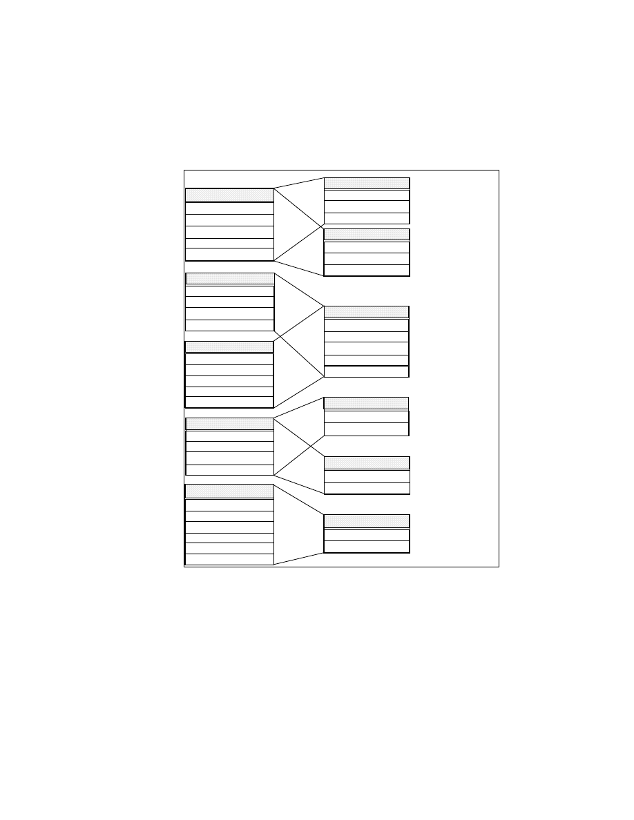
168
Getting Started with Data Warehouse and Business Intelligence
PRODUCT:
ARTICLE:
SEA SUN SPIRIT SPRAY 50 ML
LINE:
SUN SPIRIT
BRAND:
SEA
SUPPLIER: SEA SUPPLIER
Figure 35 shows the relationship between the different data sources and the
intermediate staging tables.
Figure 35. Sources for Dimension Table PRODUCT
DEPOT.SUPPLNO
DEPOT.DEPOTNO
DEPOT.SUPPLNO
DEPOT.TEXT_DEPOT
DEPOT.DEPOTNO
DEPOT.TEXT_LINE
DEPO
TNO(
6:7)=
'00'
PRODNO = 3.0
DEPO
TNO(6
:7)>'00
'
SUPPLIERS_ARTICLE.SUPPLNO
STRUC_ARTICLE.BASARTNO
SUPPLIERS_ARTICLE.DEPOTNO
STRUC_ARTICLE.DELETE_DATE
STRUC_ARTICLE.DEL_MARK
PRODNO = 3.0
BASARTNO
DE
L_
MA
RK
+
'L'
ARTICLE_TXT.BASARTNO
ARTICLE_TXT.ARTICLE.TEXT
ARTICLE_TXT.BASARTNO
ARTICLE_TXT.ARTICLE.TEXT
TX
TT
YP
NO
=1
.0
TXTT
YPNO
=2.0
SUPPLIER.SUPPLNO
SUPPLIER.NAME
ART_BRAND_TXT
SUPPL_NO
BRAND_NO
BRAND_TEXT
ART_LINE_TXT
SUPPL_NO
LINE_NO
LINE_TEXT
ART_STR_SUP
ART_NO
SUPPL_NO
DEL_MARK
BASARTNO LINE_NO
DELETE_DATE
ART_NAME_TXT
ART_NO
ART_NAME
ART_CONTENT_TXT
ART_NO
ART_CONTENT
SUPPLIER
SUPPL_NO
SUPPL_NAME
COMPNO = 3.0
FILENO
= '02'
RECTYPE = 0.0
COSTL_NEW = '07'
PRODNO = 3.0
SJVSEDB1
DEPOT
SUPPLNO
DEPOTNO
TEXT_LINE
TEXT_DEPOT
PRODNO
SJVSEDB1
STRUC_ARTICLE
BASARTNO
DEL_MARK
PRODNO
DELETE_DATE
SJVSEDB1
SUPPLIERS_ARTICLE
SUPPLNO
PRODNO
DEPOTNO
BASARTNO
DEL_MARK
SJVSEDB1
ARTICLE_TXT
BASARTNO
ARTICLE_TEXT
PRODNO
TXTTYPNO
SJVVSAM
SUPPLIER
SUPPLNO
NAME
FILENO
COMPNO
RECTYPE
COSTL_NEW

The Data Warehouse Definitions
169
The left side shows the real sources, and on the right side are the
intermediate sources. As you can see, we sometimes had to derive two
intermediate source tables from one original source. That is due to these
tables not being normalized. So, for example, we have several entries for one
article number, which had different content in the text field. These different
entries were distinguished by the value in another column. A normalized DB2
table would have these different attributes in different columns, so that only
one row would exist—that is, what we realized in the target business view
(dimension table PRODUCT).
The graphics between the tables on the left and the right show in the
intersection the where clause matching to all of the participating sources, and
in the other part the criteria to be met by the adjacent table (this can be either
source or target). So in case of the tables ’STRUC_ARTICLE’ and
’SUPPLIERS_ARTICLE’, ’BASARTNO’ is the column used for the join, and
only entries with ’PRODNO’ = 3.0 are placed into the intermediate source
table ’ART_STR_SUP’. In contrast, the ’DEL_MARK not equal ’L’ criterion
applies to the ’SUPPLIERS_ARTICLE’ table only.
Figure 36 shows how the staging tables are joined to build the final dimension
table.
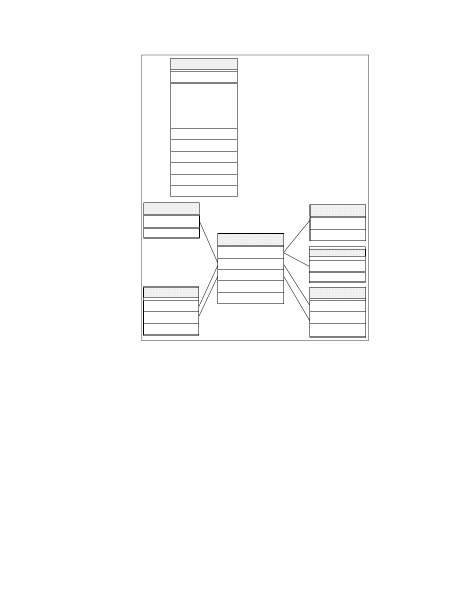
170
Getting Started with Data Warehouse and Business Intelligence
Figure 36. Dimension Table PRODUCT from Join of Intermediate Sources
6.1.2 The Second Dimension
The second dimension depicts the organization of the company. This
dimension has a hierarchy with four levels as well. The lowest level is the
store, the next one is the region, followed by company, and the highest level
is the business line.
IN
T
(L
IN
E
_
N
O
/1
0
0
)
=
IN
T
(B
R
A
N
D
_N
O
/1
0
0)
ART_CONTENT_TXT
ART_NO
ART_CONTENT
ART_NAME_TXT
ART_NO
ART_NAME
ART_BRAND_TXT
SUPPLY_NO
BRAND_TEXT
BRAND_NO
ART_STR_SUP
ART_NO
LINE_NO
SUPPLY_NO
DEL_MARK
DELETE_DATE
ART_LINE_TXT
SUPPLY_NO
LINE_TEXT
LINE_NO
SUPPLIER
SUPPLY_NO
SUPPLY_NAME
ART_BRAND_TXT.BRAND_TEXT
ART_STR_SUP.ART_NO
|| ART_LINE_TXT.LINE_TEXT
|| ART_CONTENT_TXT.ART_CONTENT
|| ART_NAME_TXT.ART_NAME
ART_STR_SUP.LINE_NO
ART_LINE_TXT.LINE_TEXT
ART_BRAND_TXT.BRAND_TEXT
SUPPLIER.SUPPL_NAME
ART_STR_SUP.SUPPL_NO
ARTICLE
ART_NAME
ART_NO
LINE_NO
BRAND_NO
LINE_NAME
BRAND_NAME
SUPPLY_NO
SUPPLY_NO
ART_BRAND_TXT.BRAND_NO

The Data Warehouse Definitions
171
Following is an example of an instance of the organization dimension:
ORGANIZATION:
STORE:
SEA WEST MARKET
REGION_NO:
604
COMPANY:
SEA WEST & CO
BUSINESS_LINE: PERFUMES
Figure 37 shows again the relationship between the various data sources for
the organization information and the consolidated staging area.
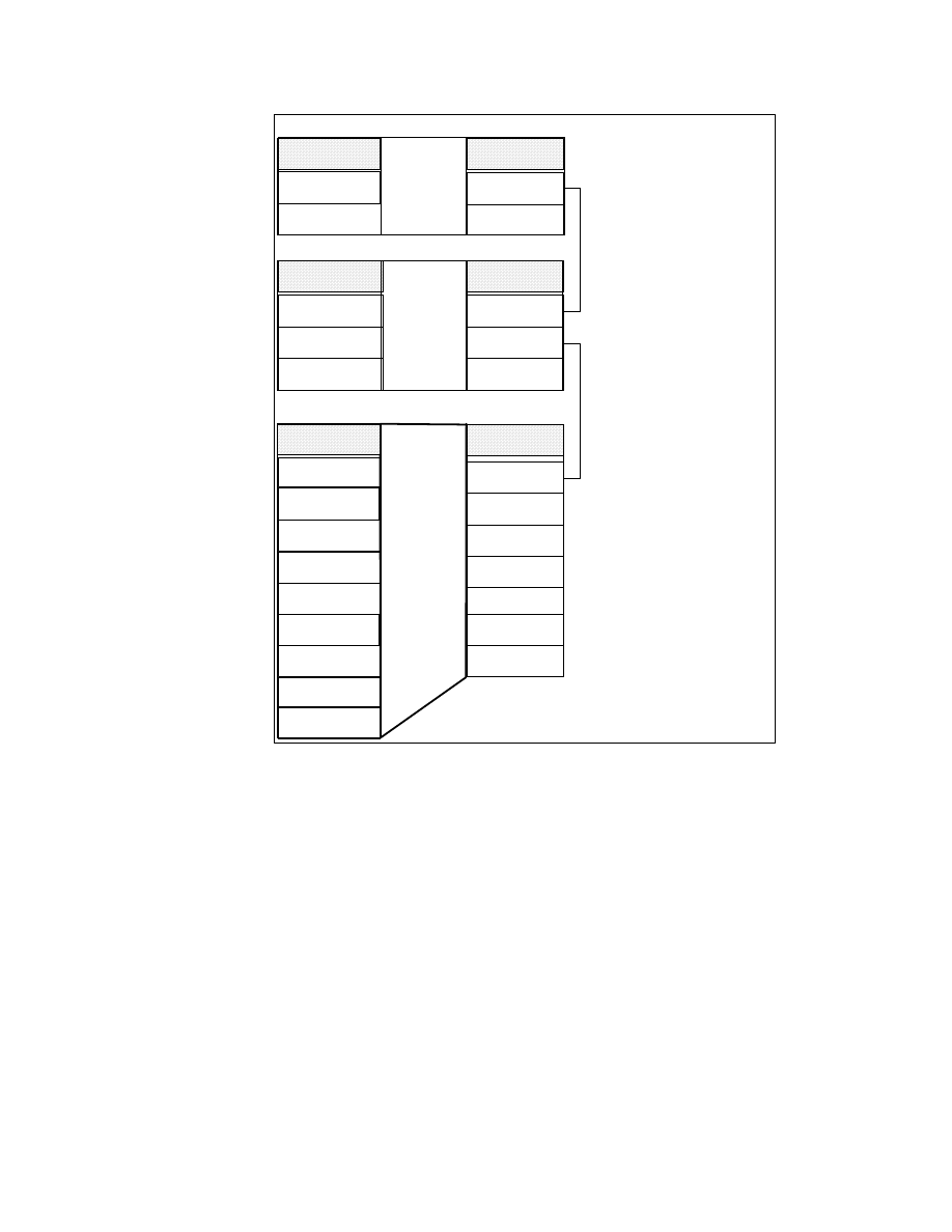
172
Getting Started with Data Warehouse and Business Intelligence
Figure 37. Sources for Dimension Table ORGANIZATION
Figure 38 shows how the intermediate staging tables are used to build the
dimension table for organization.
SJNTADD
B_Lines
BL_NAME
BL_NO
COMPNO in (12.0,
44.0,
61.0, 62.0, 63.0)
COMPANIES
COMP_NO
BL_NO
COMP_NAME
FILENO =
'01'
RECTYPE = 1.0
Business_Lines
BL_NO
SJVDLI
COMPANY_DB
NAME
COMPNO
B_LINE
COMPNO in (12.0,
44.0,
61.0, 62.0, 63.0)
STORENO<600.0
REGIONMGR
between
600 and 699
STORES.STORENO
STORES.NAME
STORES.ZIP
STORES.STREET
STORES.CITY
STORES.REGIONMGR
STORES.COMPNO
COMPANY_DB.COMPNO
COMPANY_DB.B_LINE
COMPANY_DB.NAME
BUSINESS_LINES.BL_NAME
BUSINESS_LINES.BL_NO
RECTYPE
SJVVSAM
STORES
COMPNO
ZIP
STORENO
STORENAME
STREET
CITY
REGIONMGR
FILENO
STORES
STORE_NO
STORE_NAME
ZIP
STREET
CITY
REGION_NO
COMP_NO
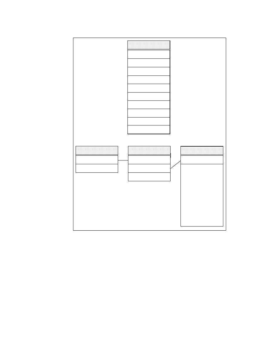
The Data Warehouse Definitions
173
Figure 38. Dimension Table ORGANIZATION from JOIN of Intermediate Sources
ORGANIZATION
STORE_NAME
STORE_NO
ZIP
REGION_NO
CITY
COMP_NO
BL_NO
COMP_NAME
BL_NAME
STREET
COMPANIES
COMP_NO
BL_NO
COMP_NAME
B_LINES
BL_NAME
BL_NO
STORES
STORE_NO
.
.
.
.
.
.
.
.
.
COMP_NO
STORES.STORE_NAME
STORES.STORE_NO
STORES.ZIP
STORES.REGION_NO
STORES.CITY
COMPANIES.COMP_NO
B_LINES.BL_NO
COMPANIES.COMP_NAME
B_LINES.BL_NAME
STORES.STREET

174
Getting Started with Data Warehouse and Business Intelligence
6.2 Technical Implementation of the Data Acquisition Process
We used Visual Warehouse to implement the data acquisition process in this
example. We implemented two different scenarios. One scenario uses the
target database including the staging tables on a DB2 UDB for AIX; the other
scenario was implemented using DB2 UDB on NT.
The administration of both target systems is done from the Windows NT
workstation ’KHANKA’, which has the Visual Warehouse server function
installed. This server function is not available on AIX.
The Visual Warehouse control database ’VWCNTL01’ resides on the server
system ’KHANKA’. The target warehouse databases are located on the
Windows NT system ’PALAU’ (SJNTDWH1) and on the AIX system ’AZOV’
(SJAXDWH1).
The transformation from the source data to the target model is defined and
managed by Visual Warehouse using Visual Warehouse Business Views
(BVs).
The following features of Visual Warehouse were used to support the data
transformation:
• Transient BVs for the staging data
• Scheduling and cascading capabilities to automate the data acquisition
process
• Work in Progress view of Visual Warehouse to monitor the execution of
the data acquisition process
• Visual Warehouse Meta Data Catalog to document and drive the data
acquisition process
The BVs for the intermediate sources can be created as transient BVs, that
is, the population of the transient BV is triggered by the target BV, and the
data is kept only temporarily until the data has arrived in the final dimension
table safely. To do this, the Transient Data check box has to be selected on
the Information folder of the Business View notebook.
This feature helps you to manage the space in the data warehouse more
efficiently, without the administrative overhead needed to get rid of temporary
result tables manually.
The actual control flow during the data acquisition process is managed with
the scheduling and cascading function of Visual Warehouse.

The Data Warehouse Definitions
175
The transient BV will be referenced by the target BV created as a dimension
table for OLAP. If this target BV is populated due to an explicit request or a
schedule, the transient BVs are populated first, then the target BV is filled,
and the transient BV will be deleted. A transient BV cannot be scheduled!
Another way to automate the population of BVs belonging to one target BV
(dimension table), is to schedule the execution of the next BV to be populated
by the one which just completed. To make sure that all the sources have been
populated before the target BV is run, you will have to set this up as a chain.
So the first BV will be populated by request, or scheduled by another event,
and the next BV will be scheduled by this one, and so on, until the target BV
is scheduled as the last one. To do this, you can select the Starts option from
the Schedule Type pulldown menu in the Schedule folder of the Business
View notebook. You can add the appropriate BV from the selection panel,
which is then displayed.
Once the BVs and the relationships between them have been defined, the
entire data acquisition process can be monitored from the work in progress
view within Visual Warehouse Administrator. Every planned, ongoing, and
finished execution of every BV is listed in this view. At any point in time, the
administrator can identify what the status of the tables in the warehouse is.
If there were errors during the execution of a BV, the details of the error
situation are logged and made accessible from this work-in-progress view as
well.
All the information that is generated during the data acquisition process—that
is, information about the structure of the data sources and target tables,
mapping information, BV descriptive and administrative information, and
statistical information about the execution of the BVs—is stored in the Visual
Warehouse meta data catalog. It can be enriched with business definitions
and can be accessed by the business analysts in order to help them
understand the content and status of the warehouse as well as to help them
to navigate within the warehouse structures.
The design and implementation of a manageable data warehouse
infrastructure is not a trivial task, many different functions are involved. A
data staging area is needed to support the transformation of the data from an
application centric model to a business centric model. The staging process
can have several steps until the final target data model is reached, depending
on the diversity of the data sources and the complexity of the transformations.
We could solve most of the requirements using Visual Warehouse in this
example.

176
Getting Started with Data Warehouse and Business Intelligence
However, in some cases, the functions provided by Visual Warehouse may
not be sufficient to address all data quality and data conversion issues. You
may have to incorporate user-written code to implement specific
transformations or you may want to use generated code from tools such as
ETI Extract and Vality Integrity to support your data acquisition and cleansing
process.
Visual Warehouse supports the integration of these other components and
allows for the control and management of these components from a single
point.

© Copyright IBM Corp. 1999
177
Appendix A. The OS/390 Environment
This appendix provides detailed information and samples of the OS/390
environment.
A.1 The IMS - DBCTL Environment
The DBCTL environment is similar to the DB/DC environment; a DL/I region
owns the databases to be processed. DL/I is part of the DBCTL environment,
although DL/I runs in its associated address space. Database Recovery
Control (DBRC) facilities, required for DBCTL, help to manage database
availability, system logging, and database recovery.
The greatest dissimilarity between DBCTL and DB/DC is that DBCTL does
not support user terminals, a master terminal, or message handling.
Therefore, no Message Processing Program (MPP) regions exist. The Batch
Message Processing (BMP) region is used only by batch applications and
utilities.
The CCTL handles message traffic and schedules application programs, all
outside the DBCTL environment. It passes database calls through the
interface to the control region, which sends the calls to DL/I and passes the
results back through the interface to the CCTL.
The information in this book that describes the IMS online system applies to
both DB/DC and DBCTL. Exceptions are noted as not applicable to DBCTL.
Figure 39 on page 178 shows an example of the DBCTL environment.

178
Getting Started with Data Warehouse and Business Intelligence
Figure 39. Example of a DBCTL Environment
A.2 The DB/DC Environment
In the DB/DC environment, data is centrally managed for applications that are
being executed concurrently and made available to terminal users. Database
Recovery Control (DBRC) facilities help to manage database availability and
system logging.
The basic unit of work is the transaction. Transaction processing consists of:
• Receiving a request for work that has been entered at a terminal. The
request is in the form of a transaction code, which identifies the kind of
work to be performed and the data needed to do it.
• Invoking a program to do the work, and preparing a response for the
terminal operator (for example, an acknowledgment of work performed or
an answer to an inquiry).
• Transmitting the response to the terminal that requested the work.
The simplest kind of transaction involves two messages: an input message
from the terminal user and an output message in return. Application programs
can also send messages to terminals other than the input source, and they
can generate transactions.
Figure 40 on page 179 represents a DB/DC environment.
MVS (or
_________ ________ ________ ________ ________
secondary)
|
|
|
|
|
|
|
console
| Control |?------------------------ÿ|
|
|
_________
| Region
|
|
|
|
|
|
|
Start
|____ÿ|
|
|
|
|
|
|
| Regions |
| (without|
BMP
|
DL/I
|
DBRC
| D | C
|
|_________|
| terminal| Region |
|
| R | C
|
| support |
|
|
| A | T
|
| or data |
|
|
|
| L
|
| communi-|
|
|
|
|
|
| cation
|
|
|
|
|
|
| facili- |
|
"
|
|
|
|
| ties)
|
|
|
|
|
|
|
|
|___ _____|___|____|_____|__|________|________|
|
_____
_________
|_________
| Log |
| Report
|
|_____|
|_________|
_____
_____

The OS/390 Environment
179
Figure 40. Example of a DB/DC Environment
A.3 Configuring the DBCTL Environment
The following sections show how the IMS/DBCTL environment at the IBM
ITSO scenario was configured.
A.3.1 Create Stage 1 Input for DBCTL System
During the initialization for start-up of the IMS on-line system, a control
program, which has been customized to your requirements, is loaded. The
input data that drives this process is a set of macro source statements. Each
statement is coded with its own parameters. The composite of all the macro
statements is termed the stage 1 input.
Six sets or groupings of macro statements make up the content of the stage 1
input. The IMSGEN macro contributes to the system configuration definition.
Within each set, individual macros specify data that is specific to a required
function or to a part of the total physical on-line configuration.
If you use the IMS DBCTL control region, you have to include your Database
Description (DBD) and Program Specification Block (PSB) information in
Stage1 input as shown in Figure 41 on page 180.
Dependent Regions
________ ________ ________ ________
|
|
|
|
|
MVS Console
_________ _______ _______ _______ _______ _______
_________
|
|
|
|
|
|
|
|
Start
|____ÿ| Control |
|
|
|
|
|
|
CTL
|
| Region
|
|
|
|
|
|
|_________|
|
|
|
|
|
|
|
|
|
|
|
|
|
|
Master Terminal |
|
|
|
|
|
|
____________
|
_____
|
|
|
|
|
|
|
Start
|_ÿ| |
| |
|
|
|
|
|
| Dependents |
| |
| |
MPP
|
MPP
|
BMP
|
IFP
|
DBRC
|
|____________|
| |DL/I | | Region | Region | Region | Region |
|
| |
| |
|
|
|
|
|
| |
| |
|
|
|
|
|
User Terminals
| |_____| |
|
|
|
|
|
____________
|
"
|
|
|
|
|
|

180
Getting Started with Data Warehouse and Business Intelligence
Figure 41. Example of DBD and PSB Specifications
This example shows three DBD entries: one for the HIDAM database, and two
for indexes for the HIDAM database. It also shows one PSB entry.
Following is a sample of the Stage1 input in the ITSO environment:
*
***********************************************************************
* INSTALL/IVP IMS 6.1
*
* SKELETON: DFSIXSC1
*
* FUNCTION: STAGE 1 SOURCE FOR A DBC SYSTEM
***********************************************************************
*
**************************************************************@SCPYRT**
*
*
*
Licensed Materials - Property of IBM
*
*
*
*
"Restricted Materials of IBM"
*
*
*
*
5655-158 (C) Copyright IBM Corp. 1989
*
*
All Rights Reserved.
*
*
*
*
US Government Users Restricted Rights -
*
*
Use, duplication or disclosure restricted by
*
*
GSA ADP schedule contract with IBM Corp.
*
*
*
**************************************************************@ECPYRT**
*
* IMSCTRL MACRO --
*
**********************************************************************
*
DATAJOINTER CLASSIC CONNECT DATABASE & APPLICATION DEFINITION
**********************************************************************
DATABASE DBD=FIRDB,ACCESS=UP
HIDAM/VSAM
DATABASE INDEX,DBD=FIRDBI,ACCESS=UP
HIDAM/VSAM INDEX
DATABASE INDEX,DBD=FIRDBS,ACCESS=UP
HIDAM/VSAM INDEX
**********************************************************************
APPLCTN PSB=PFIRDB,PGMTYPE=BATCH
HIDAM/VSAM

The OS/390 Environment
181
IMSCTRL
SYSTEM=(VS/2,(ALL,DBCTL),4.3),
X
IRLM=YES,
X
IRLMNM=IR6D,
X
CMDCHAR=/,
X
DBRC=(YES,YES),
X
DBRCNM=IVP61RC1,
X
DLINM=IVP61DL1,
X
IMSID=IMSD,
X
NAMECHK=(YES,S1),
X
MAXIO=(,015),
X
MAXREGN=(005,512K,A,A),
X
MCS=(2,7),
X
DESC=7,
X
MAXCLAS=016
*
* IMSCTF
MACRO --
*
IMSCTF SVCNO=(,203,202),
X
LOG=SNGL,
X
CPLOG=3000,
X
RDS=(3380,4096),
X
PRDR=IVP61RD3
*
* BUFPOOLS MACRO --
*
BUFPOOLS PSB=24000,
X
DMB=24000,
X
SASPSB=(4000,20000),
X
PSBW=12000
*
* SECURITY MACRO --
*
SECURITY TYPE=(AGNEXIT),
X
SECCNT=2,
X
PASSWD=YES,
X
TRANCMD=YES
**********************************************************************
*
DATAJOINTER CLASSIC CONNECT DATABASE & APPLICATION DEFINITION
**********************************************************************
DATABASE DBD=FIRDB,ACCESS=UP
HIDAM/VSAM
DATABASE INDEX,DBD=FIRDBI,ACCESS=UP
HIDAM/VSAM INDEX
DATABASE INDEX,DBD=FIRDBS,ACCESS=UP
HIDAM/VSAM INDEX
**********************************************************************
APPLCTN PSB=PFIRDB,PGMTYPE=BATCH
HIDAM/VSAM
SPACE 2
**********************************************************************
*

182
Getting Started with Data Warehouse and Business Intelligence
* IMSGEN MACRO --
*
IMSGEN ASM=(HLASM,SYSLIN),ASMPRT=OFF,
X
LKPRT=(XREF,LIST),LKSIZE=(880K,64K),LKRGN=900K,
X
SUFFIX=C,
X
SURVEY=YES,
X
MACLIB=ALL,
X
NODE=(IMS610D,
X
IMS610D,
X
IMS610D),
X
OBJDSET=IMS610D.OBJDSET,
X
PROCLIB=YES,
X
USERLIB=IMS610D.LOAD,
X
UMAC0=,
X
SYSMAC=SYS1.MACLIB,
X
MODGEN=SYS1.MODGEN,
X
UMAC1=,
X
UMAC2=,
X
UMAC3=,
X
ONEJOB=(),
X
JCL=(IMSGEN,
X
(999,POK),
X
’INSTALL’,T,
X
(CLASS=A,MSGLEVEL=(1,1),REGION=32M,NOTIFY=YOURID)),
X
SCL=(255,,(TIME=600)),
X
UJCL1=’/*JOBPARM L=999,SYSAFF=SC53
X
’,
X
UJCL2=,
X
UJCL3=,
X
UJCL4=,
X
UJCL5=
END ,
*
A.3.2 Run the IMS System Definition STAGE 1
Stage 1 is the first part of the process of defining an IMS system. Stage 1
checks input specifications and generates a series of OS/390 job steps that
are the input to stage 2.

The OS/390 Environment
183
Following is a sample of the Stage1 JCL in the ITSO environment:
//IV2C203J JOB (999,POK),
// ’INSTALL’,
// CLASS=A,MSGCLASS=T,MSGLEVEL=(1,1),
// NOTIFY=&SYSUID,
// REGION=32M
//*
/*JOBPARM L=999,SYSAFF=SC53
//*
//*********************************************************************
//* INSTALL/IVP IMS 6.1
//*
//* SKELETON: DFSIXSC3
//*
//* FUNCTION: RUN THE IMS SYSTEM DEFINITION STAGE1
//*********************************************************************
//*
//************************************************************@SCPYRT**
//*
*
//*
Licensed Materials - Property of IBM
*
//*
*
//*
"Restricted Materials of IBM"
*
//*
*
//*
5655-158 (C) Copyright IBM Corp. 1974,1996
*
//*
All Rights Reserved.
*
//*
*
//*
US Government Users Restricted Rights -
*
//*
Use, duplication or disclosure restricted by
*
//*
GSA ADP schedule contract with IBM Corp.
*
//*
*
//************************************************************@ECPYRT**
//*
//STAGE1
EXEC PGM=ASMA90,PARM=’NOOBJ,DECK’,TIME=(600)
//SYSPRINT DD SYSOUT=*
//SYSLIB
DD DISP=SHR,DSN=IMS610D.GENLIB
//
DD DISP=SHR,DSN=IMS610D.GENLIBA
//
DD DISP=SHR,DSN=IMS610D.GENLIBB
//SYSPUNCH DD DISP=SHR,
//
DSN=SW5106R.JCLLIB(IV2C301J)
//SYSUT1
DD UNIT=3390,SPACE=(CYL,(05,05)),DCB=OPTCD=C
//SYSUT2
DD UNIT=3390,SPACE=(CYL,(05,05)),DCB=OPTCD=C
//SYSUT3
DD UNIT=3390,SPACE=(CYL,(05,05)),DCB=OPTCD=C
//SYSIN
DD DISP=SHR,
//
DSN=SW5106R.JCLLIB(IV2C201T)

184
Getting Started with Data Warehouse and Business Intelligence
A.3.3 Run the IMS System Definition STAGE 2
Stage 2 is the second part of the process of defining an IMS system. Stage 2
builds IMS system libraries, execution procedures, and the IMS online control
program tailored to support the desired set of IMS functions. Stage 2 then
stores these in an IMS library.
A.3.4 Create DFSPBxxx Member
This member contains parameters updated when the IMS control region
starts. It is located in imshlq.PROCLIB, where imshlq means IMS high-level
qualifier.
Figure 42. Example of DFSPBxxx
Set "SUF" to what you specified in your Stage1 source under the parameter
"SUFFIX" of IMSGEN MACRO.
Set "IMSID" to your IMS subsystem name.
Set "ISIS" to say whether resource access security checking is to be
performed. You can control resource access and prevent an unauthorized
CCTL from connecting to the DBCTL environment using the ISIS execution
parameter. Set "ISIS" to 0 if you do not control resource access.
Set "DBRCNM" to your DBRC started procedure name.
Set "DLINM" to your DL/I started procedure name.
Set "CRC" to your command prefix name when issuing the IMS command
from the OS/390 console.
Set "IRLM" to "Y" if you use IRLM for resource locking.
Set "IRLMNM" to your primary IRLM subsystem name in case of specifying
"IRLM" to "Y".
SUF=C,
IMSID=IMSD,
ISIS=0,
LGNR=10,
DBRCNM=IVP6DRC1,
DLINM=IVP6DDL1,
PRDR=IVP6DRD1,
CRC=/,
IRLM=N,
IRLMNM=,

The OS/390 Environment
185
For more information about the parameters of DFSPBxxx, see Section 4.23,
"Parameter Descriptions", in IMS/ESA V 6 Installation, Volume 2,
GC26-8737.
Following is a sample of the DFSPBxxx member in the ITSO environment:
RES=Y,
PST=5,
SRCH=0,
DMB=048,
CIOP=,
WKAP=048,
PSBW=024,
DBWP=024,
SUF=C,
FIX=DC,
PRLD=DC,
VSPEC=DC,
BSIZ=02048,
OTHR=005,
DBFX=00010,
DBBF=00050,
FMTO=D,
AUTO=N,
IMSID=IMSD,
ISIS=0,
LGNR=10,
SSM=,
WADS=D,
ARC=01,
UHASH=,
DBRCNM=IVP6DRC1,
DLINM=IVP6DDL1,
CSAPSB=12,
DLIPSB=40,
PRDR=IVP6DRD1,
EPCB=0012,
CRC=/,
DBRSE=,
FPWP=,
SPM=,
TRACK=,
RSRMBR=,
APPLID1=,
APPLID2=,
APPLID3=,
USERVAR=,

186
Getting Started with Data Warehouse and Business Intelligence
IRLM=N,
IRLMNM=,
PIMAX=20,
PIINCR=1,
AOIP=,
AOIS=,
MAXPST=,
PREMSG=
A.3.5 Create IMS DBCTL Started Procedure
Figure 43 shows a started procedure for the IMS DBCTL control region. You
should set the "RGSUF" parameter to your suffix for the DFSPBxxx.
Figure 43. Example of IMS Started Procedure Parameter
Following is a sample of the IMS DBCTL Started Procedure in the ITSO
environment:
//
PROC RGN=2000K,SOUT=A,DPTY=’(14,15)’,
//
SYS=,SYS2=,
//
RGSUF=IV3,PARM1=,PARM2=
//IEFPROC EXEC PGM=DFSMVRC0,DPRTY=&DPTY,REGION=&RGN,
//
PARM=’DBC,&RGSUF,&PARM1,&PARM2’
//*
//*
//* THE MEANING AND MAXIMUM SIZE OF EACH PARAMETER
//* IS AS FOLLOWS:
//****************************************************
//*
RGSUF
XXX
EXEC PARM DEFAULT BLOCK SUFFIX FOR
//*
MEMBER DFSPBXXX.
//****************************************************
//*
//
PROC RGN=2000K,SOUT=A,DPTY=’(14,15)’,
//
SYS=,SYS2=,
//
RGSUF=IV3
,PARM1=,PARM2=
//IEFPROC EXEC PGM=DFSMVRC0,DPRTY=&DPTY,REGION=&RGN,
//
PARM=’DBC,&RGSUF,&PARM1,&PARM2’
//*
//*
//* THE MEANING AND MAXIMUM SIZE OF EACH PARAMETER
//* IS AS FOLLOWS:
//****************************************************
//*
RGSUF
XXX
EXEC PARM DEFAULT BLOCK SUFFIX FOR
//*
MEMBER DFSPBXXX.
//****************************************************
:

The OS/390 Environment
187
//*
PARM1 , PARM2 PARAMETERS BOTH ARE USED TO SPECIFY
//*
CHARACTER STRINGS THAT CONTAIN IMS KEYWORD
//*
PARAMETERS. I.E. PARM1=’AUTO=Y,PST=222,RES=Y’
//*
//*
ALL OF THE VALID DBCTL KEYWORD PARAMETERS
//*
ARE DESCRIBED BELOW
//****************************************************
//*
//******** CONTROL REGION SPECIFICATIONS ********
//*
RES
X
BLOCK RESIDENT (N = NO, Y = YES)
//*
PST
XXX
NUMBER OF PST’S PERMANENTLY ALLOC
//*
MAXPST XXX
MAXIMUM NUMBER OF PST’S
//*
SRCH
X
MODULE SEARCH INDICATOR FOR DIRECTED LOAD
//*
0 = STANDARD SEARCH
//*
1 = SEARCH JPA AND LPA BEFORE PDS
//*
FMTO
T = ONLINE FORMATTED DUMP WITH
//*
STORAGE IMAGE DELETIONS.
//*
TERM=NO SDUMPS ALLOWED.
//*
P = FULL ONLINE FORMATTED DUMP.
//*
TERM=NO SDUMPS ALLOWED.
//*
F = FULL ONLINE FORMATTED DUMP.
//*
TERM=NO SDUMPS NOT ALLOWED.
//*
N = NO FORMATTED DUMP, NO OFFLINE
//*
DUMP. TERM=NO SDUMPS ALLOWED.
//*
Z = NO FORMATTED DUMP, NO OFFLINE
//*
DUMP. TERM=NO SDUMPS NOT
//*
ALLOWED.
//*
(DEFAULT)
D = OFFLINE DUMP, OR ONLINE FORMAT-
//*
TED DUMP WITH STORAGE IMAGE
//*
DELETIONS IF OFFLINE DUMPING
//*
FAILS. TERM=NO SDUMPS ALLOWED.
//*
X = OFFLINE DUMP, OR ONLINE FORMAT-
//*
TED DUMP WITH STORAGE IMAGE
//*
DELETIONS IF OFFLINE DUMPING
//*
FAILS. TERM=NO SDUMPS NOT
//*
ALLOWED.
//*
M = OFFLINE DUMP, ONLINE IMS DUMP
//*
FORMATTING NOT PERMITTED
//*
TERM=NO SDUMPS ALLOWED.
//*
R = OFFLINE DUMP, ONLINE IMS DUMP
//*
FORMATTING NOT PERMITTED
//*
TERM=NO SDUMPS NOT ALLOWED.
//*
AUTO
X
Y = AUTOMATIC RESTART DESIRED
//*
N = NO AUTOMATIC RESTART
//*
IMSID
XXXX
IMS SUBSYSTEM IDENTIFIER
//*
ISIS
X
0 = NO RESOURCE ACCESS SECURITY
//*
1 = RACF RESOURCE ACCESS SECURITY

188
Getting Started with Data Warehouse and Business Intelligence
//*
2 = USER RESOURCE ACCESS SECURITY
//*
ARMRST X
Y = ALLOW MVS ARM TO RESTART
//*
N = ARM NOT RESTART IMS
//*
IRLM
X
Y = YES, N = NO
//*
IRLMNM XXXX
IRLM SUBSYSTEM NAME
//*
SSM
XXXX
EXT SUBSYSTEM PROCLIB MEMBER ID
//*
WADS
X
SINGLE OR DUAL WADS,S=SINGLE,D=DUAL
//*
ARC
XX
AUTOMATIC ARCHIVE.
//*
0 = NOT AUTOMATIC
//*
1-99 = AUTOMATIC
//*
UHASH
XXXXXXXX USER HASH MODULE NAME
//*
DBRCNM XXXXXXXX DBRC PROCLIB MEMBER NAME
//*
DLINM
XXXXXXXX DL/I PROCLIB MEMBER NAME
//*
PRDR
XXXXXXXX IMSRDR PROCLIB MEMBER NAME
//*
DBRSE
XXXXXXXX 8 CHAR DBCTL RSENAME
//*
CRC
X
COMMAND RECOGNITION CHARACTER
//*
CMDMCS X
COMMAND SECURITY OPTION
//*
R=RACF COMMAND SECURITY
//*
C=DFSCCMD0 COMMAND SECURITY
//*
B=RACF AND DFSCCMD0 CMD SEC
//*
PREMSG X
PREFIX MESSAGE OPTION
//*
N=NO DFS000I PREFIX
//*
Y=DEFAULT, DFS000I PREFIX
//*
PIMAX
XXXXXX ENQ/DEQ POOL MAXIMUM BYTES
//*
PIINCR XXXXXX ENQ/DEQ POOL INCREMENT
//*
AOIS
X
ICMD SECURITY OPTION
//*
YEAR4
X
N = 2-DIGIT DATE
//*
Y = 4-DIGIT DATE
//*
//******** FDR PARAMETER *****************************
//*
//*
FDRMBR
XX
SUFFIX FOR FDR MEMBER IN
//*
IMS610D.PROCLIB
//*
//******** FAST PATH PARAMETERS ********
//*
//*
BSIZ
XXX
DATA BASE BUFFER SIZE
//*
OTHR
XXX
NUMBER OF OUTPUT THREADS
//*
DBFX
XXX
SYSTEM ALLOCATION OF DATA BASE BUFFERS TO BE
//*
FIXED AT START OF 1ST FAST PATH DEP REGION
//*
DBBF
XXX
NUMBER OF DATABASE BUFFERS
//*
LGNR
XX
NUMBER OF LOG ENTRIES IN DEDB BUFFERHEADER
//*
//******** RSR PARAMETERS *************************
//*
//*
RSRMBR XX
SUFFIX FOR RSR MEMBER
//*
TRACK
XXX
NO = NO RECOVERY TRACKING DONE

The OS/390 Environment
189
//*
RLT = RECOVERY TRACKING DONE
//*
DLT = DATABASE TRACKING DONE
//*
//******** STORAGE POOL VALUES IN K, M OR G ******
//*
DMB
XXXXXX DMB POOL SIZE
//*
CIOP
XXXXXX CIOP POOL UPPER LIMIT
//*
WKAP
XXXXXX WORKING STORAGE BUFFER POOL SIZE
//*
PSBW
XXXXXX PSB WORK POOL SIZE
//*
DBWP
XXXXXX DATABASE WORK POOL SIZE
//*
CSAPSB XXXXXX DLISAS: CSA PSB POOL SIZE
//*
DLIPSB XXXXXX DLISAS: DLI PSB POOL SIZE
//*
EPCB
XXXXXX EPCB POOL SIZE
//*
FPWP
XXXXXX FP WORK POOL UPPER LIMIT
//*
AOIP
XXXXXX AOI POOL UPPER LIMIT
//*
//******** MEMBER SUFFIXES **********************
//*
//*
SUF
X
LAST CHARACTER OF CTL PROGRAM LOAD
//*
MODULE MEMBER NAME
//*
FIX
XX
2 CHARACTER FIX PROCEDURE MODULE SUFFIX
//*
PRLD
XX
2 CHARACTER PROCLIB MEMBER SUFFIX FOR PRELOAD
//*
VSPEC
XX
2 CHARACTER BUFFER POOL SPEC MODULE SUFFIX
//*
SPM
XX
STORAGE POOL OPTIONS (DFSSPMXX)
//***********************************************
//*
//STEPLIB
DD DSN=IMS610D.&SYS2.RESLIB,DISP=SHR
//
DD DSN=DJX.V2R1M01.SDJXLOAD,DISP=SHR
//PROCLIB
DD DSN=IMS610D.&SYS2.PROCLIB,DISP=SHR
//*
//***************************************************
//* IN ORDER TO START A DEPENDENT REGION, MODIFIED
//* START-UP JCL IS WRITTEN FROM INTERNAL STORAGE TO
//* THE INTERNAL READER.
//*
//IMSIRD
DD SYSOUT=(A,INTRDR)
//*
//*********** DASD
LOGGING DD CARDS *************
//* THE FOLLOWING DD CARDS DESCRIBE THE DASD LOGGING
//* OLDS AND WADS. THESE CARDS ARE FOR EXAMPLE ONLY.
//* ALL OLDS AND WADS DATA SETS MAY BE DYNAMICALLY
//* ALLOCATED.
DD CARDS ARE NOT REQUIRED.
//* THE OLDS AND WADS TO BE USED DURING STARTUP MUST
//* BE SPECIFIED VIA OLDSDEF AND WADSDEF CONTROL
//* STATEMENTS IN THE DFSVSMXX MEMBER OF IMS PROCLIB.
//* THE ACTUAL SELECTION OF OLDS AND WADS MUST BE
//* TAILORED TO INSTALLATION REQUIREMENTS.
THE OLDS
//* AND WADS MUST BE PREDEFINED BY A SET UP JOB.

190
Getting Started with Data Warehouse and Business Intelligence
//* THE BLOCK SIZE OF ALL OLDS MUST BE THE SAME.
//* THE BLOCK SIZE AND DEVICE TYPE OF ALL WADS MUST
//* BE THE SAME.
AT LEAST 3 PRIMARY OLDS AND 1 WADS
//* MUST BE AVAILABLE FOR STARTUP.
THE BLOCK SIZE
//* SHOULD NOT BE SPECIFIED IN THIS JCL.
THE LOGGER
//* WILL GET THE BLOCK SIZE FROM THE VTOC.
//*
//DFSOLP00 DD DSN=IMS610D.&SYS.OLP00,DISP=SHR
//DFSOLP01 DD DSN=IMS610D.&SYS.OLP01,DISP=SHR
//DFSOLP02 DD DSN=IMS610D.&SYS.OLP02,DISP=SHR
//DFSOLP03 DD DSN=IMS610D.&SYS.OLP03,DISP=SHR
//DFSOLP04 DD DSN=IMS610D.&SYS.OLP04,DISP=SHR
//DFSOLP05 DD DSN=IMS610D.&SYS.OLP05,DISP=SHR
//*
//DFSOLS00 DD DSN=IMS610D.&SYS.OLS00,DISP=SHR
//DFSOLS01 DD DSN=IMS610D.&SYS.OLS01,DISP=SHR
//DFSOLS02 DD DSN=IMS610D.&SYS.OLS02,DISP=SHR
//DFSOLS03 DD DSN=IMS610D.&SYS.OLS03,DISP=SHR
//DFSOLS04 DD DSN=IMS610D.&SYS.OLS04,DISP=SHR
//DFSOLS05 DD DSN=IMS610D.&SYS.OLS05,DISP=SHR
//*
//DFSWADS0 DD DSN=IMS610D.&SYS.WADS0,DISP=SHR
//DFSWADS1 DD DSN=IMS610D.&SYS.WADS1,DISP=SHR
//*
//IMSACBA
DD DSN=IMS610D.&SYS2.ACBLIBA,DISP=SHR
//IMSACBB
DD DSN=IMS610D.&SYS2.ACBLIBB,DISP=SHR
//MODBLKSA DD DSN=IMS610D.&SYS2.MODBLKSA,DISP=SHR
//MODBLKSB DD DSN=IMS610D.&SYS2.MODBLKSB,DISP=SHR
//MODSTAT
DD DSN=IMS610D.&SYS.MODSTAT,DISP=SHR
//******** SYSTEM REQUIRED DD CARDS **************
//*
//SYSUDUMP DD SYSOUT=&SOUT,
//
DCB=(LRECL=125,RECFM=FBA,BLKSIZE=3129),
//
SPACE=(6050,300,,,ROUND)
//IMSRDS
DD DSN=IMS610D.&SYS.RDS,DISP=SHR
//MATRIXA
DD DSN=IMS610D.&SYS2.MATRIXA,DISP=SHR
//MATRIXB
DD DSN=IMS610D.&SYS2.MATRIXB,DISP=SHR
//PRINTDD
DD SYSOUT=&SOUT
//*
//****** EXTERNAL SUBSYSTEM DD CARDS
***********
//*
//* USER MAY OPTIONALLY ADD THE DFSESL DD CARD
//* FOR EXTERNAL SUBSYSTEM CONNECTION.
//*
//************ DATA BASE DD CARDS ***************
//*
//* USER MAY OPTIONALLY SUPPLY THE DD STATEMENTS

The OS/390 Environment
191
//* FOR THE ON-LINE DATA BASES TO BE
//* INSERTED HERE PRIOR TO ATTEMPTING
//* AN ON-LINE SYSTEM EXECUTION USING
//* THIS PROCEDURE.
//* IF NO DD STATEMENTS ARE SUPPLIED FOR
//* A DATA BASE, IMS ASSUMES THAT THIS
//* DATA BASE HAS BEEN DESCRIBED THROUGH
//* THE DFSMDA MACRO.
//* IF THE USER WILL BE EXECUTING WITH THE DL/I
//* SAS OPTION, THESE DD STATEMENTS SHOULD BE ADDED
//* TO THE DLISAS PROCLIB MEMBER OR DESCRIBED
//* THROUGH THE DFSMDA MACRO.
A.3.6 Create IMS DL/I Started Procedure
This procedure initializes a DL/I (Data Language I) separate address space
(DLISAS).
You have to use a DL/I separate address space (DLISAS) to contain code,
control blocks, and buffers for full-function databases for the IMS DBCTL
control region.
The IMS control program automatically initiates the DL/I address space. If
either the control or DL/I address space terminates, the other is automatically
terminated.
For using the IMS DBCTL control region, you have to add DD statements for
your IMS Databases in the DL/I started procedure.
Following is a sample of the IMS DL/I Started Procedure in the ITSO
environment:
//
PROC RGN=3072K,DPTY=’(14,15)’,SOUT=A,
//
IMSID=IMSD,SYS2=
//IEFPROC EXEC PGM=DFSMVRC0,REGION=&RGN,
//
DPRTY=&DPTY,PARM=(DLS,&IMSID)
//****************************************************
//*
//STEPLIB
DD DSN=IMS610D.&SYS2.RESLIB,DISP=SHR
//PROCLIB
DD DSN=IMS610D.&SYS2.PROCLIB,DISP=SHR
//****************** ACBLIB **************************
//*
//* THE SPECIFICATION OF THE ACBLIB DATASETS
//* IN THE DLI/SAS REGION PROCEDURE MUST
//* CORRESPOND EXACTLY WITH THE SPECIFICATION
//* IN THE CONTROL REGION JCL

192
Getting Started with Data Warehouse and Business Intelligence
//*
//IMSACBA
DD DSN=IMS610D.&SYS2.ACBLIBA,DISP=SHR
//IMSACBB
DD DSN=IMS610D.&SYS2.ACBLIBB,DISP=SHR
//SYSUDUMP DD SYSOUT=&SOUT
//SYSABEND DD SYSOUT=&SOUT
//************ DATA BASE DD CARDS ********************
//*
//* USER MAY OPTIONALLY SUPPLY THE DD STATEMENTS
//* FOR THE ON-LINE DATA BASES TO BE
//* INSERTED HERE PRIOR TO ATTEMPTING
//* AN ON-LINE SYSTEM EXECUTION USING
//* THIS PROCEDURE.
//* IF NO DD STATEMENTS ARE SUPPLIED FOR
//* A DATA BASE, IMS ASSUMES THAT THIS
//* DATA BASE HAS BEEN DESCRIBED THROUGH
//* THE DFSMDA MACRO.
//*
//FIRDB
DD DSN=SJVSAM.FIRMEN.STAMM,DISP=SHR
//FIRDBI
DD DSN=SJVSAM.FIRMEN.STAMM.PRIIX,DISP=SHR
//FIRDBS
DD DSN=SJVSAM.FIRMEN.STAMM.SECIX,DISP=SHR
A.3.7 Create IMS DBRC Started Procedure
DBRC is responsible for the following tasks:
1. This first group of tasks are those performed automatically through the
interaction of DBRC and IMS (including utilities):
• Controlling logs for IMS
• Recording recovery information in the RECON (Recovery Control
data set)
• Verifying that database utilities have the correct input
• Controlling the recovery of registered databases
• Controlling the data sharing environment by maintaining authorization
information for the control and serialization of access to shared
databases
2. These tasks are performed when you request them by passing commands
to DBRC:
• Recording recovery information in the RECON
• Generating JCL for various IMS utilities and generating user-defined
output (Use GENJCL commands to perform these operations.)

The OS/390 Environment
193
• Listing the information in the RECONs; use LISTcommands to list this
information
IMS automatically starts the DBRC procedure with an OS/390 START
command during control region initialization. This procedure specifies
parameters for the DBRC region.
To include the DBRC procedure during system generation, you must copy the
skeletal procedure that IMS generates in IMS.PROCLIB to SYS1.PROCLIB.
The member name must match the name specified on the DBRCNM
parameter in the IMSCTRL macro or the applicable EXEC procedure. If
DBRCNM is specified in more than one place, or if DBRCNM is not explicitly
specified, the following order of precedence applies:
• DBRCNM=DBRC is the default.
• DBRCNM=name in the IMSCTRL macro overrides the default.
• DBRCNM=name defined in a DFSPBxxx member in IMS.PROCLIB
overrides the IMSCTRL macro setting.
• DBRCNM=name defined in a JCL EXEC parameter overrides the
IMS.PROCLIB member setting.
Following is a sample of the IMS DBRC Started Procedure in the ITSO
environment:
//
PROC RGN=2048K,DPTY=’(14,15)’,SOUT=A,
//
IMSID=IMSD,SYS2=
//IEFPROC EXEC PGM=DFSMVRC0,REGION=&RGN,
//
DPRTY=&DPTY,PARM=(DRC,&IMSID)
//****************************************************
//*
//STEPLIB
DD DSN=IMS610D.&SYS2.RESLIB,DISP=SHR
//PROCLIB
DD DSN=IMS610D.&SYS2.PROCLIB,DISP=SHR
//JCLOUT
DD SYSOUT=(A,INTRDR)
//JCLPDS
DD DSN=IMS610D.&SYS2.PROCLIB,DISP=SHR
//SYSUDUMP DD SYSOUT=&SOUT
//SYSABEND DD SYSOUT=&SOUT
//*
//************ DBRC RECON DD CARDS *******************
//*
//* USER MAY OPTIONALLY SUPPLY THE DD CARDS
//* REQUIRED FOR THE DBRC RECON DATA SET.
//* IF NO DD STATEMENTS ARE SUPPLIED FOR RECON
//* DATASETS, IMS ASSUMES THAT THE DATASETS
//* HAVE BEEN DESCRIBED THROUGH THE DFSMDA MACRO.

194
Getting Started with Data Warehouse and Business Intelligence
//*
A.3.8 Allocate RECON Data Sets
DBRC stores recovery-related information in a set of VSAM KSDSs called the
RECON (Recovery Control) data sets.
Three RECONs should be defined when you install DBRC. The first two
RECONs are active data sets, the third one is a spare. The second active
data set is a copy of the first. For most purposes, you can think of the two
active RECONs as if they were a single data set, the RECON, or simply
RECON.
Allocate RECON data sets for the IMS DBCTL system.
Following is a sample of the RECON Data Sets Allocation JCL in the ITSO
environment:
//IV2G101J JOB (999,POK),
// ’INSTALL’,
// CLASS=A,MSGCLASS=T,MSGLEVEL=(1,1),
// NOTIFY=&SYSUID,
// REGION=32M
//*
/*JOBPARM L=999,SYSAFF=SC53
//*
//*********************************************************************
//* INSTALL/IVP IMS 6.1
//*
//* SKELETON: DFSIXSG0
//*
//* FUNCTION: ALLOCATE DATA SETS NEEDED FOR THE DBCTL SYSTEM IVP
//*********************************************************************
//*
//************************************************************@SCPYRT**
//*
*
//*
Licensed Materials - Property of IBM
*
//*
*
//*
"Restricted Materials of IBM"
*
//*
*
//*
5655-158 (C) Copyright IBM Corp. 1974,1996
*
//*
All Rights Reserved.
*
//*
*
//*
US Government Users Restricted Rights -
*
//*
Use, duplication or disclosure restricted by
*
//*
GSA ADP schedule contract with IBM Corp.
*

The OS/390 Environment
195
//*
*
//************************************************************@ECPYRT**
//*
//* SCRATCH DATA SETS
//*
//SCRATCH
EXEC PGM=IDCAMS,DYNAMNBR=200
//SYSPRINT DD SYSOUT=*
//SYSIN
DD *
DELETE IMS610D.RECON1 CLUSTER
DELETE IMS610D.RECON2 CLUSTER
DELETE IMS610D.RECON3 CLUSTER
//*
//* ALLOCATE DATA SETS
//*
//ALLOCATE EXEC PGM=IDCAMS,DYNAMNBR=200
//SYSPRINT DD SYSOUT=*
//SYSIN
DD *
DEFINE CLUSTER(
-
NAME(IMS610D.RECON1)
-
FREESPACE(20 20)
-
INDEXED
-
KEYS(32 0)
-
RECORDSIZE(4086 32600)
-
SHAREOPTIONS(3 3)
-
RECOVERY
-
NOERASE
-
SPANNED
-
NOREUSE
-
UNORDERED
-
UNIQUE
-
VOLUMES(TOTIM3)
-
CYL(3 1)
-
)
-
DATA(
-
NAME(IMS610D.RECON1.DATA)
-
)
-
INDEX(
-
NAME(IMS610D.RECON1.INDX)
-
)
DEFINE CLUSTER(
-
NAME(IMS610D.RECON2)
-
FREESPACE(20 20)
-
INDEXED
-
KEYS(32 0)
-
RECORDSIZE(4086 32600)
-
SHAREOPTIONS(3 3)
-
RECOVERY
-

196
Getting Started with Data Warehouse and Business Intelligence
NOERASE
-
SPANNED
-
NOREUSE
-
UNORDERED
-
UNIQUE
-
VOLUMES(TOTIM3)
-
CYL(3 1)
-
)
-
DATA(
-
NAME(IMS610D.RECON2.DATA)
-
)
-
INDEX(
-
NAME(IMS610D.RECON2.INDX)
-
)
DEFINE CLUSTER(
-
NAME(IMS610D.RECON3)
-
FREESPACE(20 20)
-
INDEXED
-
KEYS(32 0)
-
RECORDSIZE(4086 32600)
-
SHAREOPTIONS(3 3)
-
RECOVERY
-
NOERASE
-
SPANNED
-
NOREUSE
-
UNORDERED
-
UNIQUE
-
VOLUMES(TOTIM3)
-
CYL(3 1)
-
)
-
DATA(
-
NAME(IMS610D.RECON3.DATA)
-
)
-
INDEX(
-
NAME(IMS610D.RECON3.INDX)
-
)
//*
A.3.9 Register DBRC Information
Figure 44 shows you an example of RECON records registration.

The OS/390 Environment
197
Figure 44. Example of RECON Records Registration
In this example, you would need to add at least the following three types of
statements:
INIT.RECON
After allocating the RECONs, use the INIT.RECON command to initialize the
RECON header and control records. This command is only valid for an empty,
uninitialized RECON. If the initialization job fails before it has completed
successfully, delete and redefine the data sets before rerunning it.
Set SSID to IMS subsystem ID.
INIT.DB
Use an INIT.DB command to create a database record in RECON and
register the database with DBRC. The database must be registered in
RECON before you can initialize a new DBDS area with the INIT.DBDS
command. You can also use the INIT.DB command to specify the level of
database sharing.
Set DBD to the name of your DBD. You need INIT.DB statements for each
DBD.
INIT.RECON SSID(IMSD)
-
00041006
FORCER CHECK17 SHARECTL NONEW
-
00042006
DASDUNIT(3390) TAPEUNIT(3490)
00043006
INIT.DB
DBD(FIRDB)
SHARELVL(2)
00050004
INIT.DBDS
DBD(FIRDB)
DDN(FIRDB)
GENMAX(2)
-
00060004
REUSE
DSN(SJVSAM.FIRMEN.STAMM)
-
00070004
ICJCL(ICJCL)
OICJCL(OICJCL) -
00080004
RECOVJCL(RECOVJCL)
00090004
INIT.IC
DBD(FIRDB)
DDN(FIRDB) -
00100004
ICDSN(SJVSAM.FIRDB.IC)
00110005
INIT.DB
DBD(FIRDBI)
SHARELVL(2)
00130004
INIT.DBDS
DBD(FIRDBI)
DDN(FIRDBI)
GENMAX(2)
-
00140004
REUSE
DSN(SJVSAM.FIRMEN.STAMM.PRIIX)
-
00150004
ICJCL(ICJCL)
OICJCL(OICJCL) -
00160004
RECOVJCL(RECOVJCL)
00170004
INIT.IC
DBD(FIRDBI)
DDN(FIRDBI) -
00180004
ICDSN(SJVSAM.FIRDB.PRIIX.IC)
00190005
:
:

198
Getting Started with Data Warehouse and Business Intelligence
INIT.DBDS
Use an INIT.DBDS command to initiate DBRC’s control of the recovery of a
DBDS area. The INIT.DBDS command causes a DBDS record to be written in
RECON. The DBDS record must exist for any of the other commands to work
for a given DBDS area. Before creating the DBDS record, DBRC examines
the IMS DBDLIB data set to:
• Verify that the DBDS area exists.
• Obtain the DBDS’s data set identifier (DSID), its data set organization, and
its database organization.
Set DBD to the name of your DBD for the DBDS.
Set DDN to the ddname of your DBDS.
See the manual, IMS/ESA V6 DBRC Guide and Reference, SC26-8733-01 for
more information about each of the command parameters.
Following is a JCL sample of the Register DBRC Information in the ITSO
environment:
//INIT04
EXEC PGM=DSPURX00
//STEPLIB
DD
DSN=IMS610D.RESLIB,DISP=SHR
//SYSPRINT DD
SYSOUT=*
//IMS
DD
DSN=IMS610D.DBDLIB,DISP=SHR
//
DD
DSN=IMS610D.PSBLIB,DISP=SHR
//SYSIN
DD
*
INIT.RECON SSID(IMSD)
-
FORCER CHECK17 SHARECTL NONEW
-
DASDUNIT(3390) TAPEUNIT(3490)
INIT.DB
DBD(FIRDB)
SHARELVL(2)
INIT.DBDS
DBD(FIRDB)
DDN(FIRDB)
GENMAX(2)
-
REUSE
DSN(SJVSAM.FIRMEN.STAMM)
-
ICJCL(ICJCL)
OICJCL(OICJCL) -
RECOVJCL(RECOVJCL)
INIT.IC
DBD(FIRDB)
DDN(FIRDB) -
ICDSN(SJVSAM.FIRDB.IC)
INIT.DB
DBD(FIRDBI)
SHARELVL(2)
INIT.DBDS
DBD(FIRDBI)
DDN(FIRDBI)
GENMAX(2)
-
REUSE
DSN(SJVSAM.FIRMEN.STAMM.PRIIX)
-
ICJCL(ICJCL)
OICJCL(OICJCL) -
RECOVJCL(RECOVJCL)
INIT.IC
DBD(FIRDBI)
DDN(FIRDBI) -
ICDSN(SJVSAM.FIRDB.PRIIX.IC)
INIT.DB
DBD(FIRDBS)
SHARELVL(2)
INIT.DBDS
DBD(FIRDBS)
DDN(FIRDBS)
GENMAX(2)
-
REUSE
DSN(SJVSAM.FIRMEN.STAMM.SECIX)
-

The OS/390 Environment
199
ICJCL(ICJCL)
OICJCL(OICJCL) -
RECOVJCL(RECOVJCL)
INIT.IC
DBD(FIRDBS)
DDN(FIRDBS) -
ICDSN(SJVSAM.FIRDB.SECIX.IC)
/*
INIT.CAGRP
GRPNAME(CAGRPSJ)
GRPMAX(2) REUSE -
GRPMEM((FIRDB,FIRDB))
INIT.CA
GRPNAME(CAGRPSJ) CADSN(SW5106R.*.CADSN1) -
VOLLIST(TOTDB7)
FILESEQ(4)
INIT.CA
GRPNAME(CAGRPSJ) CADSN(SW5106R.*.CADSN2) -
VOLLIST(TOTDB8)
A.4 Data Creation
A.4.1 IMS Definitions
This section describes how you would define the IMS database. The sample
definitions are for the HIDAM database.
A.4.1.1 Generate DBD
The sample JCL to generate DBDs is as follows:
//DBDGEN PROC MBR=TEMPNAME,SOUT=A,RGN=0M,SYS2=
//C
EXEC PGM=ASMA90,REGION=&RGN,
//
PARM=’OBJECT,NODECK,NODBCS’
//SYSLIB
DD DSN=IMS610D.&SYS2.MACLIB,DISP=SHR
//SYSLIN
DD UNIT=SYSDA,DISP=(,PASS),
//
SPACE=(80,(100,100),RLSE),
//
DCB=(BLKSIZE=80,RECFM=F,LRECL=80)
//SYSPRINT DD SYSOUT=&SOUT,DCB=BLKSIZE=1089,
//
SPACE=(121,(300,300),RLSE,,ROUND)
//SYSUT1
DD UNIT=SYSDA,DISP=(,DELETE),
//
SPACE=(CYL,(10,5))
//L
EXEC PGM=IEWL,PARM=’XREF,LIST’,
//
COND=(0,LT,C),REGION=2M
//SYSLIN
DD DSN=*.C.SYSLIN,DISP=(OLD,DELETE)
//SYSPRINT DD SYSOUT=&SOUT,DCB=BLKSIZE=1089,
//
SPACE=(121,(90,90),RLSE)
//SYSLMOD
DD DISP=SHR,
//
DSN=IMS610D.&SYS2.DBDLIB(&MBR)
//SYSUT1
DD UNIT=(SYSDA,SEP=(SYSLMOD,SYSLIN)),
//
SPACE=(1024,(100,10),RLSE),DISP=(,DELETE)
//
PEND
//*
//DBDGEN
EXEC DBDGEN,MBR=FIRDB
//C.SYSIN
DD
*

200
Getting Started with Data Warehouse and Business Intelligence
DBD
NAME=FIRDB,
*
ACCESS=HIDAM
DATASET DD1=FIRDB,
*
DEVICE=3380,
*
BLOCK=(4096),
*
FRSPC=(0,0)
SEGM
NAME=FAST,
*
BYTES=130,PARENT=0,
*
RULES=(,LAST),POINTER=(TB)
FIELD NAME=(FIRMA,SEQ,U),TYPE=P,
*
START=1,BYTES=2
FIELD NAME=FILLER,TYPE=C,
*
START=3,BYTES=128
LCHILD NAME=(FIRDBI$,FIRDBI),
*
POINTER=INDX
SEGM
NAME=FABU,
*
BYTES=1500,PARENT=((FAST,SNGL)),
*
RULES=(,LAST),POINTER=(TB)
FIELD NAME=(KZ,SEQ,U),TYPE=C,
*
START=1,BYTES=1
FIELD NAME=FILLER1,TYPE=C,
*
START=2,BYTES=255
FIELD NAME=FILLER2,TYPE=C,
*
START=257,BYTES=256
FIELD NAME=FILLER3,TYPE=C,
*
START=513,BYTES=256
FIELD NAME=FILLER4,TYPE=C,
*
START=769,BYTES=256
FIELD NAME=FILLER5,TYPE=C,
*
START=1025,BYTES=256
FIELD NAME=FILLER6,TYPE=C,
*
START=1281,BYTES=220
SEGM
NAME=FALI,
*
BYTES=500,PARENT=((FAST,SNGL)),
*
RULES=(,LAST),POINTER=(TB)
FIELD NAME=(PROGNR,SEQ,U),TYPE=C,
*
START=1,BYTES=8
FIELD NAME=PROGFA,TYPE=P,
*
START=0009,BYTES=002
FIELD NAME=FILLER1,TYPE=C,
*
START=11,BYTES=246
FIELD NAME=FILLER2,TYPE=C,
*
START=257,BYTES=244
LCHILD NAME=(FIRDBS$,FIRDBS),
*
POINTER=INDX
XDFLD NAME=LISTNR,
*
SEGMENT=FALI,
*

The OS/390 Environment
201
SRCH=(PROGNR,PROGFA)
DBDGEN
FINISH
END
/*
//*
//DBDGEN
EXEC DBDGEN,MBR=FIRDBI
//C.SYSIN
DD
*
PRINT NOGEN
DBD
NAME=FIRDBI,
*
ACCESS=INDEX
DATASET DD1=FIRDBI,
*
DEVICE=3380,
*
BLOCK=291,RECORD=14
SEGM
NAME=FIRDBI$,
*
BYTES=2,PARENT=0,
*
RULES=(,LAST)
FIELD NAME=(FIRMA,SEQ,U),TYPE=C,
*
START=1,BYTES=2
LCHILD NAME=(FAST,FIRDB),
*
INDEX=FIRMA,
*
POINTER=SNGL
DBDGEN
FINISH
END
/*
//*
//DBDGEN
EXEC DBDGEN,MBR=FIRDBS
//C.SYSIN
DD
*
PRINT NOGEN
DBD
NAME=FIRDBS,
*
ACCESS=INDEX
DATASET DD1=FIRDBS,
*
DEVICE=3380,
*
BLOCK=185,RECORD=22
SEGM
NAME=FIRDBS$,
*
BYTES=10,PARENT=0,
*
RULES=(,LAST)
FIELD NAME=(LISTNR,SEQ,U),TYPE=C,
*
START=1,BYTES=10
LCHILD NAME=(FALI,FIRDB),
*
INDEX=LISTNR,
*
POINTER=SNGL
DBDGEN
FINISH
END
/*

202
Getting Started with Data Warehouse and Business Intelligence
A.4.1.2 Allocate the VSAM file for IMS
The sample JCL to allocate VSAM files is as follows:
//DEFINE
EXEC PGM=IDCAMS
//*STEPCAT
DD DSNAME=IMSCAT1,DISP=SHR
//SYSPRINT
DD SYSOUT=A
//SYSABEND
DD SYSOUT=A
//*VSA
DD UNIT=SYSDA,DISP=OLD,VOL=SER=VSIMS
//SYSIN
DD *
DELETE SJVSAM.FIRMEN.STAMM
DELETE SJVSAM.FIRMEN.STAMM.PRIIX
DELETE SJVSAM.FIRMEN.STAMM.SECIX
DEFINE
CLUSTER
-
(NAME(SJVSAM.FIRMEN.STAMM)
-
NONINDEXED
-
SHR(3 3)
-
CISZ(4096)
-
RECSZ(4089 4089)
-
CYL(2 1)
-
VOL(TOTDB9))
-
CAT(SJVSAM)
DEFINE
CLUSTER
-
(NAME(SJVSAM.FIRMEN.STAMM.PRIIX)
-
INDEXED
-
SHR(3 3)
-
RECSZ(14 14)
-
CYL(2 1)
-
KEYS(2 5)
-
FSPC(0 0)
-
VOL(TOTDB9))
-
DATA(
-
CISZ(4096))
-
CAT(SJVSAM)
DEFINE
CLUSTER
-
(NAME(SJVSAM.FIRMEN.STAMM.SECIX)
-
INDEXED
-
SHR(3 3)
-
RECSZ(22 22)
-
CYL(2 1)
-
KEYS(10 5)
-
FSPC(0 0)
-
VOL(TOTDB9))
-
DATA(
-
CISZ(4096))
-
CAT(SJVSAM)

The OS/390 Environment
203
//*
A.4.1.3 Generate PSB
The sample JCL to generate PSB is as follows:
//PSBGEN PROC MBR=TEMPNAME,SOUT=*,RGN=0M,SYS2=
//C
EXEC PGM=ASMA90,REGION=&RGN,
//
PARM=’OBJECT,NODECK,NODBCS’
//SYSLIB
DD DSN=IMS610D.&SYS2.MACLIB,DISP=SHR
//SYSLIN
DD UNIT=SYSDA,DISP=(,PASS),
//
SPACE=(80,(100,100),RLSE),
//
DCB=(BLKSIZE=80,RECFM=F,LRECL=80)
//SYSPRINT DD SYSOUT=&SOUT,DCB=BLKSIZE=1089,
//
SPACE=(121,(300,300),RLSE,,ROUND)
//SYSUT1
DD UNIT=SYSDA,DISP=(,DELETE),
//
SPACE=(CYL,(10,5))
//L
EXEC PGM=IEWL,PARM=’XREF,LIST’,
//
COND=(0,LT,C),REGION=20M
//SYSLIN
DD DSN=*.C.SYSLIN,DISP=(OLD,DELETE)
//SYSPRINT DD SYSOUT=&SOUT,DCB=BLKSIZE=1089,
//
SPACE=(121,(90,90),RLSE)
//SYSLMOD
DD DISP=SHR,
//
DSN=IMS610D.&SYS2.PSBLIB(&MBR)
//SYSUT1
DD UNIT=(SYSDA,SEP=(SYSLMOD,SYSLIN)),
//
SPACE=(1024,(100,10),RLSE),DISP=(,DELETE)
//
PEND
/*
//PSBGEN
EXEC PSBGEN,MBR=PFIRDB
//C.SYSIN
DD
*
PCB
TYPE=DB,DBDNAME=FIRDB,
*
PROCOPT=GOTP,KEYLEN=10
SENSEG
NAME=FAST,PARENT=0
SENSEG
NAME=FABU,PARENT=FAST
SENSEG
NAME=FALI,PARENT=FAST
PCB
TYPE=DB,DBDNAME=FIRDBI,
*
PROCOPT=G,KEYLEN=2
SENSEG
NAME=FIRDBI$,PARENT=0
PCB
TYPE=DB,DBDNAME=FIRDBS,
*
PROCOPT=GE,KEYLEN=10
SENSEG
NAME=FIRDBS$,PARENT=0
PSBGEN
LANG=COBOL,PSBNAME=PFIRDB
END
/*

204
Getting Started with Data Warehouse and Business Intelligence
A.4.1.4 Generate ACB
If you use the IMS DBCTL control region, you have to generate ACB. The
sample JCL to generate ACB is as follows:
//ACBGEN PROC
SOUT=*,COMP=,RGN=256K
//G
EXEC
PGM=DFSRRC00,PARM=’UPB,&COMP’,REGION=&RGN
//SYSPRINT DD
SYSOUT=&SOUT
//STEPLIB
DD
DSN=IMS610D.RESLIB,DISP=SHR
//DFSRESLB DD
DSN=IMS610D.RESLIB,DISP=SHR
//IMS
DD
DSN=IMS610D.PSBLIB,DISP=SHR
//
DD
DSN=IMS610D.DBDLIB,DISP=SHR
//IMSACB
DD
DSN=IMS610D.ACBLIB,DISP=OLD
//SYSUT3
DD
UNIT=SYSDA,SPACE=(80,(100,100))
//SYSUT4
DD
UNIT=SYSDA,SPACE=(256,(100,100)),DCB=KEYLEN=8
//COMPCTL
DD
DSN=IMS610D.PROCLIB(DFSACBCP),DISP=SHR
//
PEND
//*
//ACBGEN
EXEC ACBGEN
//SYSIN
DD
*
BUILD PSB=(PFIRDB)
A.4.2 DB2 Definitions
A.4.2.1 Create Storage Group
Create a storage group from SPUFI, or by any other method, as shown in the
following example:
CREATE STOGROUP SJDB1SG1
VOLUMES (TOTDB9)
VCAT DB2V510I ;
A.4.2.2 Create Database
Create a database from SPUFI, or by any other method, as shown in the
following example:
CREATE DATABASE SJ390DB1
STOGROUP SJDB1SG1
BUFFERPOOL BP1 ;
A.4.2.3 Create Tablespaces
Create tablespaces from SPUFI or any other methods. The following are the
sample DMLs for each table.

The OS/390 Environment
205
WGRARTST003
CREATE TABLESPACE SJDB1TS1
IN SJ390DB1
USING STOGROUP SJDB1SG1
PRIQTY 1024
SECQTY 1024
ERASE NO
PCTFREE 05
LOCKSIZE PAGE
BUFFERPOOL BP1
CLOSE NO
;
ORGSTRUC
CREATE TABLESPACE SJDB1TS2
IN SJ390DB1
USING STOGROUP SJDB1SG1
PRIQTY 10240
SECQTY 4096
ERASE NO
PCTFREE 20
LOCKSIZE PAGE
BUFFERPOOL BP1
CLOSE NO
;
DEPOT
CREATE TABLESPACE SJDB1TS3
IN SJ390DB1
USING STOGROUP SJDB1SG1
PRIQTY 2048
SECQTY 512
ERASE NO
PCTFREE 05
LOCKSIZE PAGE
BUFFERPOOL BP1
CLOSE NO ;
ARTTXT
CREATE TABLESPACE SJDB1TS4
IN SJ390DB1
USING STOGROUP SJDB1SG1
PRIQTY 40980
SECQTY 10240
ERASE NO
PCTFREE 20
LOCKSIZE PAGE
BUFFERPOOL BP1
CLOSE NO
; .

206
Getting Started with Data Warehouse and Business Intelligence
BASART
CREATE TABLESPACE SJDB1TS5
IN SJ390DB1
USING STOGROUP SJDB1SG1
PRIQTY 16384
SECQTY 4096
ERASE NO
PCTFREE 05
LOCKSIZE PAGE
BUFFERPOOL BP1
CLOSE NO
;
SUPPLART
CREATE TABLESPACE SJDB1TS6
IN SJ390DB1
USING STOGROUP SJDB1SG1
PRIQTY 32768
SECQTY 8192
ERASE NO
PCTFREE 05
LOCKSIZE PAGE
BUFFERPOOL BP1
CLOSE NO
;
STRARTDAT
CREATE TABLESPACE SJDB1TS7
IN SJ390DB1
USING STOGROUP SJDB1SG1
PRIQTY 20800
SECQTY 5120
ERASE NO
PCTFREE 05
LOCKSIZE PAGE
BUFFERPOOL BP1
CLOSE NO
;
STRUCART
CREATE TABLESPACE SJDB1TS8
IN SJ390DB1
USING STOGROUP SJDB1SG1
PRIQTY 40960
SECQTY 10240
ERASE NO
PCTFREE 20
LOCKSIZE PAGE
BUFFERPOOL BP1
CLOSE NO
;

The OS/390 Environment
207
SELLDAY003
CREATE TABLESPACE SJDB1TS9
IN SJ390DB1
USING STOGROUP SJDB1SG1
PRIQTY 819200
SECQTY 204800
ERASE NO
PCTFREE 15
LOCKSIZE PAGE
BUFFERPOOL BP1
CLOSE NO
;
A.4.2.4 Create Tables
You must consider referential integrity when creating tables. According to the
relationship desired, create the tables in order. In our case, we had to create
the tables in the following sequence.
WGRARTST003
CREATE TABLE WGRARTST003
(COMPANY
DECIMAL(3,0)
NOT NULL,
WAREGROUP
DECIMAL(5,0)
NOT NULL,
WGR_DESCR
CHAR(60)
NOT NULL,
CREATE_DATE
DATE
NOT NULL,
CHANGE_DATE
DATE
,
DELETE_DATE
DATE
,
USER_NAME
CHAR(20)
NOT NULL,
PRIMARY KEY
(COMPANY,
WAREGROUP)) IN SJ390DB1.SJDB1TS1 ;
CREATE UNIQUE INDEX WGRASTST003IX ON WGRARTST003
(COMPANY
ASC,
WAREGROUP
ASC) ;
ORGSTRUC
CREATE TABLE ORGSTRUC
(GRPNO
DECIMAL(3,0)
NOT NULL,
COMPNO
DECIMAL(3,0)
NOT NULL,
PRCRNGNO
DECIMAL(3,0)
NOT NULL,
LOCNO
DECIMAL(3,0)
NOT NULL,
PRIMARY KEY
(GRPNO,
COMPNO,
PRCRNGNO,
LOCNO)) IN SJ390DB1.SJDB1TS2;

208
Getting Started with Data Warehouse and Business Intelligence
CREATE UNIQUE INDEX ID_ORGANISATIONSTR ON ORGSTRUC
(GRPNO
ASC,
COMPNO
ASC,
PRCRNGNO
ASC,
LOCNO
ASC ) ;
DEPOT
CREATE TABLE DEPOT
(GRPNO
DECIMAL(3,0)
NOT NULL,
COMPNO
DECIMAL(3,0)
NOT NULL,
PRCRNGNO
DECIMAL(3,0)
NOT NULL,
LOCNO
DECIMAL(3,0)
NOT NULL,
SUPPLNO
DECIMAL(13,0)
NOT NULL,
DEPOTNO
DECIMAL(7,0)
NOT NULL,
SORT_DEPOT
DECIMAL(3,0)
NOT NULL,
SORT_LINE
DECIMAL(3,0)
NOT NULL,
TEXT_DEPOT
CHAR(30)
NOT NULL,
TEXT_LINE
CHAR(30)
NOT NULL,
CREATE_DATE
DATE
NOT NULL,
DELETE_DATE
DATE
,
CALC_FACTOR
DECIMAL(5,3)
,
PRIMARY KEY
(GRPNO,
COMPNO,
PRCRNGNO,
LOCNO,
SUPPLNO,
DEPOTNO)) IN SJ390DB1.SJDB1TS3;
ALTER TABLE DEPOT
FOREIGN KEY BELONGS_
(GRPNO,
COMPNO,
PRCRNGNO,
LOCNO
)
REFERENCES ORGSTRUC ;
CREATE UNIQUE INDEX DEPOTIX ON DEPOT
(GRPNO
ASC,
COMPNO
ASC,
PRCRNGNO
ASC,
LOCNO
ASC,
SUPPLNO
ASC,
DEPOTNO
ASC) ;

The OS/390 Environment
209
ARTTXT
CREATE TABLE ARTTXT
(BASARTNO
DECIMAL(13,0)
NOT NULL,
GRPNO
DECIMAL(3,0)
NOT NULL,
COMPNO
DECIMAL(3,0)
NOT NULL,
PRCRNGNO
DECIMAL(3,0)
NOT NULL,
LOCNO
DECIMAL(3,0)
NOT NULL,
TEXTTYPNO
DECIMAL(2,0)
NOT NULL,
ARTICLETEXT
CHAR(45)
NOT NULL,
PRIMARY KEY
(BASARTNO,
GRPNO,
COMPNO,
PRCRNGNO,
LOCNO,
TEXTTYPNO)) IN SJ390DB1.SJDB1TS4;
CREATE UNIQUE INDEX ARTTXTIX ON ARTTXT
(BASARTNO
ASC,
GRPNO
ASC,
COMPNO
ASC,
PRCRNGNO
ASC,
LOCNO
ASC,
TEXTTYPNO
ASC)
CLUSTER
USING STOGROUP SJDB1SG1
PRIQTY 10240
SECQTY 5120 ;
ALTER TABLE ARTTXT
FOREIGN KEY HAS
(BASARTNO,
GRPNO,
COMPNO,
PRCRNGNO,
LOCNO
)
REFERENCES STRUCART ;
BASART
CREATE TABLE BASART
(BASARTNO
DECIMAL(13,0)
NOT NULL,
BASARTDESC
CHAR(45)
NOT NULL,
CONTENS
CHAR(7)
,
CREATE_DATE
DATE
NOT NULL,
CHANGE_DATE
DATE
,
BASARTDELDAT
DATE
,
BASARTSTRTDAT
DATE
NOT NULL,

210
Getting Started with Data Warehouse and Business Intelligence
MCONTENS
DECIMAL(3,0)
,
HEADARTNO
DECIMAL(13,0)
,
OWN_BRAND
DECIMAL(1,0)
,
DISP
DECIMAL(1,0)
,
WG1
DECIMAL(5,0)
,
WG2
DECIMAL(5,0)
,
WG3
DECIMAL(5,0)
,
WG4
DECIMAL(5,0)
,
WG5
DECIMAL(5,0)
,
COLORNO
DECIMAL(3,0)
NOT NULL,
PRIMARY KEY
(BASARTNO)) IN SJ390DB1.SJDB1TS5 ;
CREATE UNIQUE INDEX BASARTNO ON BASART
(BASARTNO
ASC
) ;
SUPPLART
CREATE TABLE SUPPLART
(SUPPLNO
DECIMAL(13,0)
NOT NULL,
BASARTNO
DECIMAL(13,0)
NOT NULL,
GRPNO
DECIMAL(3,0)
NOT NULL,
COMPNO
DECIMAL(3,0)
NOT NULL,
PRCRNGNO
DECIMAL(3,0)
NOT NULL,
LOCNO
DECIMAL(3,0)
NOT NULL,
DEL_MARK
CHAR(1)
,
DELETE_DATE
DATE
,
CHANGE_DATE
DATE
,
SUPPLARTCREDAT
DATE
NOT NULL,
SORT_ID
DECIMAL(13,0)
,
ORD_WEEK
DECIMAL(2,0)
,
ORD_DAY
DECIMAL(3,0)
,
PRLIST
CHAR(1)
,
CONDLIST
CHAR(1)
,
BILLACCNT
DECIMAL(2,0)
,
COMM_MARK
DECIMAL(2,0)
,
DELVR_KEY
DECIMAL(2,0)
,
DELVR_UNIT
DECIMAL(8,3)
NOT NULL,
SUPPL_UNIT
DECIMAL(8,3)
NOT NULL,
CONTENS
CHAR(7)
,
SUPPLARTTXT
CHAR(45)
,
SUPPLPATH
DECIMAL(3,0)
NOT NULL,
ORDERNO
CHAR(13)
,
SUPPLARTOUTDAT
DATE
NOT NULL,
DEPOTNO
DECIMAL(7,0)
NOT NULL,
DELVRTIME
DECIMAL(4,1)
,
SUPPLARTNO
CHAR(20)
,

The OS/390 Environment
211
PRIMARY KEY
(SUPPLNO,
BASARTNO,
GRPNO,
COMPNO,
PRCRNGNO,
LOCNO)) IN SJ390DB1.SJDB1TS6 ;
CREATE UNIQUE INDEX SUPPLARTIX ON SUPPLART
(SUPPLNO
ASC,
BASARTNO
ASC,
GRPNO
ASC,
COMPNO
ASC,
PRCRNGNO
ASC,
LOCNO
ASC)
CLUSTER
USING STOGROUP SJDB1SG1
PRIQTY 10240
SECQTY 5120 ;
CREATE INDEX SUP_IND1 ON SUPPLART
(SUPPLNO
ASC,
SUPPLARTNO
ASC,
GRPNO
ASC,
COMPNO
ASC,
PRCRNGNO
ASC,
LOCNO
ASC
) ;
CREATE INDEX SUP_IND2 ON SUPPLART
(SUPPLNO
ASC,
ORDERNO
ASC,
GRPNO
ASC,
COMPNO
ASC,
PRCRNGNO
ASC,
LOCNO
ASC
) ;
CREATE INDEX SUPE_IND3 ON SUPPLART
(BASARTNO
ASC,
SUPPLNO
ASC
) ;
ALTER TABLE SUPPLART
FOREIGN KEY IS_AVAIL
(BASARTNO,
GRPNO,
COMPNO,
PRCRNGNO,
LOCNO
)
REFERENCES STRUCART ;

212
Getting Started with Data Warehouse and Business Intelligence
STRARTDAT
CREATE TABLE STRARTDAT
(BASARTNO
DECIMAL(13,0)
NOT NULL,
GRPNO
DECIMAL(3,0)
NOT NULL,
COMPNO
DECIMAL(3,0)
NOT NULL,
PRCRNGNO
DECIMAL(3,0)
NOT NULL,
LOCNO
DECIMAL(3,0)
NOT NULL,
STRADATTODATE
DATE
NOT NULL,
BUYERNO
DECIMAL(3,0)
,
NO_LABEL
DECIMAL(5,0)
,
SELL_UNIT
DECIMAL(8,3)
NOT NULL,
CONT_TYPE
CHAR(2)
,
OS_ID
DECIMAL(2,0)
,
TAXNO
DECIMAL(3,0)
NOT NULL,
WGRNO
DECIMAL(5,0)
NOT NULL,
STRADATFROMDAT
DATE
NOT NULL,
TOV_WGR
DECIMAL(2,0)
,
OSUNIT
DECIMAL(8,3)
,
PRIMARY KEY
(BASARTNO,
GRPNO,
COMPNO,
PRCRNGNO,
LOCNO,
STRADATTODATE)) IN SJ390DB1.SJDB1TS7;
CREATE UNIQUE INDEX STRARTDATIX ON STRARTDAT
(BASARTNO
ASC,
GRPNO
ASC,
COMPNO
ASC,
PRCRNGNO
ASC,
LOCNO
ASC,
STRADATTODATE
ASC)
CLUSTER
USING STOGROUP SJDB1SG1
PRIQTY 10240
SECQTY 5120 ;
CREATE INDEX STD_IND1 ON STRARTDAT
(WGRNO
ASC,
BASARTNO
ASC,
GRPNO
ASC,
COMPNO
ASC,
PRCRNGNO
ASC,
LOCNO
ASC,
STRADATTODATE
ASC
)
USING STOGROUP SJDB1SG1
PRIQTY 10240
SECQTY 5120 ;

The OS/390 Environment
213
COMMENT ON TABLE STRARTDAT IS
’ARTICLE STRUCTURE DATA’ ;
ALTER TABLE STRARTDAT
FOREIGN KEY DESCRIB_
(BASARTNO,
GRPNO,
COMPNO,
PRCRNGNO,
LOCNO
)
REFERENCES STRUCART ;
STRUCART
CREATE TABLE STRUCART
(BASARTNO
DECIMAL(13,0)
NOT NULL,
GRPNO
DECIMAL(3,0)
NOT NULL,
COMPNO
DECIMAL(3,0)
NOT NULL,
PRCRNGNO
DECIMAL(3,0)
NOT NULL,
LOCNO
DECIMAL(3,0)
NOT NULL,
DEL_MARK
CHAR(1)
,
CREATE_DATE
DATE
,
DELETE_DATE
DATE
,
PRIMARY KEY
(BASARTNO,
GRPNO,
COMPNO,
PRCRNGNO,
LOCNO)) IN SJ390DB1.SJDB1TS8;
CREATE UNIQUE INDEX STRUCARTIX ON STRUCART
(BASARTNO
ASC,
GRPNO
ASC,
COMPNO
ASC,
PRCRNGNO
ASC,
LOCNO
ASC)
CLUSTER
USING STOGROUP SJDB1SG1
PRIQTY 10240
SECQTY 5120 ;
ALTER TABLE STRUCART
FOREIGN KEY REFERS__
(BASARTNO)
REFERENCES BASART ;
ALTER TABLE STRUCART
FOREIGN KEY BELONGS_
(GRPNO,
COMPNO,
PRCRNGNO,
LOCNO
)

214
Getting Started with Data Warehouse and Business Intelligence
REFERENCES ORGSTRUC ;
SELLDAY003
CREATE TABLE SELLDAY003
(DATE
DATE
NOT NULL,
BASARTNO
DECIMAL(13,0)
NOT NULL,
LOCATION
DECIMAL(4,0)
NOT NULL,
COMPANY
DECIMAL(3,0)
NOT NULL,
DEPTNO
DECIMAL(3,0)
NOT NULL,
PIECES
DECIMAL(7,0)
NOT NULL,
IN_PRC
DECIMAL(11,2)
NOT NULL,
OUT_PRC
DECIMAL(11,2)
NOT NULL,
TAX
DECIMAL(11,2)
NOT NULL,
NO_CUST
DECIMAL(7,0)
NOT NULL,
WGRNO
DECIMAL(5,0)
NOT NULL,
SUPPLNO
DECIMAL(7,0)
NOT NULL,
TRANSFER_DATE
TIMESTAMP
NOT NULL,
PROCESS_DATE
TIMESTAMP
NOT NULL)
IN SJ390DB1.SJDB1TS9;
CREATE INDEX ID_LOCATION03 ON SELLDAY003
(LOCATION
ASC,
BASARTNO
ASC
)
USING STOGROUP SJDB1SG1
PRIQTY 20480
SECQTY 5120 ;
COMMENT ON TABLE SELLDAY003 IS
’DAILY SELLINGS COMPANY 003’ ;
A.4.3 VSAM Definitions
A.4.3.1 Create User Catalog for VSAM Files
//DSNTCAT EXEC PGM=IDCAMS
//SYSPRINT DD
SYSOUT=*
//SYSUDUMP DD
SYSOUT=*
//CAT
DD
UNIT=3390,DISP=OLD,VOL=SER=TOTCAT
//SYSIN
DD
*
DEFINE UCAT
-
( NAME(CATALOG.SW5106R.VTOTCAT)
-
FILE(CAT)
-
CYLINDERS(2 1)
-
VOL(TOTCAT)
-
ICFCATALOG
)
-
DATA
-
( CYLINDERS (1 1)
)
-
INDEX
-
( CYLINDERS (1 1)
)

The OS/390 Environment
215
DEFINE ALIAS
-
( NAME(SJVSAM)
-
RELATE(CATALOG.SW5106R.VTOTCAT))
A.4.3.2 Allocate VSAM File
//STP98
EXEC PGM=IDCAMS
//SYSPRINT
DD SYSOUT=*
//SYSABEND
DD SYSOUT=*
//SYSIN
DD *
DEFINE
CLUSTER (NAME(SJVSAM.SDAT03)
-
IMBED
-
FSPC(37 4)
-
INDEXED
-
KEYS (13 1)
-
SHR (2 3) )
-
DATA (CISZ(2048)
-
RECSZ (636 636)
-
NAME (SJVSAM.SDAT03.DATA)
-
CYL(1070 100)
-
VOLUMES (TOTDB9) )
-
INDEX (CISZ(3584)
-
NAME (SJVSAM.SDAT03.INDEX)
-
TRK(25 20)
-
VOLUMES (TOTDB9) )
-
CATALOG (SJVSAM)
//*
A.4.3.3 Reload VSAM File
//ROADVSM EXEC PGM=IDCAMS
//SYSPRINT
DD SYSOUT=*
//SYSABEND
DD SYSOUT=*
//SOURCE
DD DSN=DSF$EXP,LABEL=(,SL),
//
UNIT=(B3F,,DEFER),DISP=OLD,VOL=SER=BB1112
//SYSIN
DD *
IMPORT -
INFILE(SOURCE)
-
OUTDATASET(SJVSAM.SDAT03)
-
INTOEMPTY
-
OBJECTS( -
(STAMM.DATEI03 -
NEWNAME(SJVSAM.SDAT03) -
VOLUMES(TOTDB9) ) -
) -
CATALOG(SJVSAM)
//*

216
Getting Started with Data Warehouse and Business Intelligence
A.4.4 Classic Connect Definitions
A.4.4.1 Data Server Configuration File
The sample configuration file is provided from djxhlq.SDJXCONF(DJXDSCF).
’djxhlq’ is a high level qualifier for DataJoiner Classic Connect.
***********************************************************************
***
***
***
CLASSIC CONNECT DATA SERVER CONFIGURATION
***
***
(DJXDSCF)
***
***
***
***
THIS FILE CONTAINS CONFIGURATION DATA REQUIRED
***
***
FOR THE OPERATION OF THE CLASSIC CONNECT DATA
***
***
SERVER ON MVS.
***
***
***
***
THE FILE IS ORGANIZED AS A SERIES OF ENTRIES EACH
***
***
OF WHICH CONSISTS OF A KEYWORD AND VALUE PAIR
***
***
SEPARATED BY A REQUIRED "=" SIGN.
ORDER OF THE
***
***
ENTRIES IS NOT IMPORTANT, EXCEPT WHERE NOTED.
***
***
MAXIMUM LENGTH OF AN ENTRY IS 80 CHARACTERS PER
***
***
LINE, WITH A MAXIMUM PARAMETER LENGTH OF 255
***
***
CHARACTERS, SPANNED BY THE BACKSLASH CONTINUATION
***
***
CHARACTER -
***
***
***
NOTE: WHEN EDITING CONFIGURATION MEMBERS ENSURE THAT ***
***
"NUM OFF" IS SPECIFIED. IF THE CONFIGURATION
***
***
CONTAINS SEQUENCE NUMBER, UNKNOWN CONFIGURATION
***
***
PARAMETERS, OR INVALID SUB-PARAMETER VALUES THE
***
***
DATA SERVER WILL NOT RUN.
***
***
***
***
PLEASE REFER TO CLASSIC CONNECT DOCUMENTATION FOR
***
***
ADDITIONAL INFORMATION ON SPECIFIC PARAMETERS.
***
***
***
***********************************************************************
*
* THE FOLLOWING 2 SERVICE INFO ENTRIES ARE REQUIRED SERVICES
SERVICE INFO ENTRY = DJXCNTL CNTL 0 1 1 100 4 5M 5M NO_DATA
SERVICE INFO ENTRY = DJXLOG LOGGER 1 1 1 100 4 5M 5M NO_DATA
*
**************************************************************
*
* QUERY PROCESSOR SERVICE INFO ENTRY
*
THE LAST SUBPARAMETER POINTS TO A QP SERVICE CONFIGURATION FILE
SERVICE INFO ENTRY = DJXQP DJXSAMP 2 1 2 50 4 5M 5M DJXQPCF
SERVICE INFO ENTRY = DJXQP MVSCC
2 1 2 100 4 5M 5M DJXQPCF
*
**************************************************************

The OS/390 Environment
217
*
* ALL IMS INTERFACE SIE’S MUST BE PLACED IN THE CONFIGURATION FILE
*
ABOVE XM CONNECTION HANDLER SIE.
IMS INITIALIZATION FAILURE
*
MAY OCCUR IF NOT.
*
* IMS DBB/BMP INTERFACE SERVICE INFO ENTRY
*SERVICE INFO ENTRY = DJXIMSIF IMS
2 0 1 1 4 5M 5M NO_DATA
*
* IMS DRA INTERFACE SERVICE INFO ENTRY
*
REFER TO CLASSIC CONNECT DOCUMENTATION FOR DETAILED
*
INFORMATION ON LAST SUBPARAMETER
*SERVICE INFO ENTRY = DJXDRA IMS
2 0 1 10 4 5M 5M SF,DRAUSER,DEFPSB
SERVICE INFO ENTRY = DJXDRA IMS
2 1 1 10 4 5M 5M SJ,YOURID,PFIRDB
*
**************************************************************
*
* XM CONNECTION HANDLER SERVICE INFO ENTRY
*
REFER TO CLASSIC CONNECT DOCUMENTATION FOR DETAILED
*
INFORMATION ON LAST SUBPARAMETER
*SERVICE INFO ENTRY = DJXINIT XMNT 2 0 1 100 4 5M 5M XM1/DJX/DJX
*
* TCP/IP CONNECTION HANDLER SERVICE INFO ENTRY
*
REFER TO CLASSIC CONNECT DOCUMENTATION FOR DETAILED
*
INFORMATION ON LAST SUBPARAMETER
*SERVICE INFO ENTRY = DJXINIT TCPIP 2 0 1 100 4 5M 5M
*TCP/111.111.111.111/SOCKET#
SERVICE INFO ENTRY = DJXINIT TCPIP 2 1 1 100 4 5M 5M
TCP/9.12.14.223/3500
*
*
TCP/IP SYSTEM FILE HIGH LEVEL QUALIFIER AND SUBSYSTEM NAME
*TASK PARAMETERS = =TCPIP_PREFIX=HLQUAL =TCPIP_MACH=TCPIP
TASK PARAMETERS = =TCPIP_PREFIX=TCPIPMVS.SC53 =TCPIP_MACH=TCPIPMVS
*
* SNA CONNECTION HANDLER SERVICE INFO ENTRY
*
REFER TO CLASSIC CONNECT DOCUMENTATION FOR DETAILED
*
INFORMATION ON LAST SUBPARAMETER
*SERVICE INFO ENTRY = DJXINIT LU62 2 0 1 100 4 5M 5M
*
VTM//SERVERLU//DJXTP
**************************************************************
*
* WLM USER EXIT INTERFACE INITIALIZATION SERVICE INFO ENTRY
*SERVICE INFO ENTRY = DJXWLM WLM01 2 1 1 1 4 5M 5M
*
DJXSX06 SUBSYS=JES SUBSYSNM=DJX01
*
* THE FOLLOWING PARAMETER ACTIVATES THE SAF (SECURITY) SYSTEM EXIT
*SAF EXIT = DJXSX04 IMS CLASS=PIMS
*

218
Getting Started with Data Warehouse and Business Intelligence
* THE FOLLOWING PARAMETER ACTIVATES THE SMF (REPORTING) SYSTEM EXIT
*SMF EXIT = DJXSX02 RECTYPE=255,SYSID=JES2
*
*************************************************************
*
*
MISC REQUIRED PARAMETERS
*
MESSAGE POOL SIZE = 16777216
*
NL = US ENGLISH
NL CAT = DD:ENGCAT
*
* IF YOU ARE NOT ALLOWING UPDATES TO THE CATALOG FILES WHILE
* ANY DATA SERVERS ARE ACCESSING THE CATALOG FILES, CHANGE THE
* VALUE TO A ONE.
THE CATALOG FILES WILL ONLY BE OPENED DURING
* QP INITIALIZATION RATHER THAN DURING EACH QUERY OPEN CURSOR
*
STATIC CATALOGS = 0
A.4.4.2 Data Server Star ted JCL for DRA
The sample configuration file is provided from djxhlq.SDJXSAMP(DJXDRA).
//DJXDRA
JOB (999,POK),’INSTALL’,NOTIFY=&SYSUID,
//
CLASS=A,MSGCLASS=T,TIME=1439,
//
REGION=2M,MSGLEVEL=(1,1)
//*
DJXDRA
PROVIDE VALID JOB CARD
//********************************************************************
//*
*
//*
LICENSED MATERIALS
*
//*
5655-A41
*
//*
(C) COPYRIGHT CROSS ACCESS CORPORATION
*
//*
1993,1998 ALL RIGHTS RESERVED.
*
//*
US GOVERNMENT USERS RESTRICTED RIGHTS -
*
//*
USE, DUPLICATION OR DISCLOSURE RESTRICTED.
*
//*
*
//********************************************************************
//*
*
//*
DJXDRA
*
//*
SAMPLE DATA SERVER JCL
*
//*
IMS DATA ACCESS USING THE DRA INTERFACE
*
//*
*
//*
1) IF THIS DATA SERVER IS TO BE RUN AS A BATCH JOB:
*
//*
PROVIDE A JOB CARD THAT IS VALID FOR YOUR SITE.
*
//*
*
//*
IF THIS DATA SERVER IS TO BE RUN AS A BATCH JOB THAT WILL *
//*
BE AUTOMATICALLY DISPATCHED BY AN ENTERPRISE SERVER:
*
//*
ENSURE THAT THE JOBNAME IS 6 OR LESS CHARACTERS LONG,
*

The OS/390 Environment
219
//*
AND IS SUFFIXED BY &DJXJSFX AS IN THE FOLLOWING EXAMPLE:*
//*
//JOBNAM&DJXJSFX JOB (ACCT),ABCDEF,CLASS=A.........
*
//*
(THE ENTERPRISE SERVER REPLACES &DJXJSFX WITH A
*
//*
TWO DIGIT NUMBER TO ENSURE A UNIQUE JOBNAME.)
*
//*
*
//*
IF THIS DATA SERVER IS TO BE RUN AS A STARTED TASK,
*
//*
REMOVE THE PEND AND EXEC STATEMENTS FROM THE END OF
*
//*
THIS MEMBER.
*
//*
*
//*
2) IF THIS DATA SERVER IS GOING TO BE STARTED MANUALLY AND
*
//*
NOT AUTOMATICALLY DISPATCHED BY AN ENTERPRISE SERVER,
*
//*
CHANGE PARM1 PARM TO NULL AS IN THE FOLLOWING EXAMPLE:
*
//*
//DJXDBB
PROC PARM1=’’,
.....
*
//*
*
//*
3) CHANGE DJX PARM TO CLASSIC CONNECT HIGH LEVEL QUALIFIER
*
//*
4) CHANGE CRUN PARM TO THE NETVIEW C RUNTIME LIBRARY HLQ
*
//*
5) CHANGE CONFIG PARM TO THE APPROPRIATE CONFIG MEMBER
*
//*
6) SEE NOTE REGARDING RGN PARAMETER
*
//*
7) PROVIDE APPROPRIATE DATASET NAMES IN THE DJXCAT AND
*
//*
DJXINDX DD STATEMENTS.
THIS DATA SERVER CAN ONLY PROCESS *
//*
QUERIES AGAINST TABLES DEFINED IN THE META DATA CATALOG
*
//*
FILES REFERENCED BY THESE TWO DD STATEMENTS.
*
//*
8) IF ACCESSING TABLE(S) THAT WERE DEFINED USING DD NAME
*
//*
REFERENCE(S) AS OPPOSED TO DATASET NAME REFERENCE(S), THE *
//*
APPROPRIATE DD STATEMENT(S) MUST ALSO BE INCLUDED.
IF
*
//*
ALL TABLES SERVICED BY THIS DATA SERVER WERE DEFINED WITH *
//*
DATASET NAME REFERENCES, NO DD STATEMENTS NEED TO BE
*
//*
INCLUDED (DYNAMIC FILE ALLOCATION IS USED).
*
//*
*
//********************************************************************
//DJXDRA
PROC PARM1=’&DJXPRM1’,
COMM PARM FROM ENTERPRISE SERVER
//
DJX=’DJX’,
CLASSIC CONNECT HLQ
//
CRUN=’RUNTIMEC.V1R2M0’, NETVIEW C RUNTIME LIB HLQ
//
SOUT=’*’,
SYSOUT CLASS
//
CONFIG=DJXDSCF,
DATA SERVER CONFIG FILE
//
IMS=IMS610D,
IMS SYSTEM DATASET HLQ
//
RGN=0M
REGION SIZE
//********************************************************************
//*
IF YOUR SITE LIMITS THE AMOUNT OF MEMORY ALLOCATED TO A REGION *
//*
WHEN ZERO MEG IS SPECIFIED, YOU NEED TO ENSURE THAT
*
//*
A LARGE ENOUGH REGION IS ACTUALLY ALLOCATED.
*
//*
THE REGION SIZE MUST BE COORDINATED WITH THE MESSAGE POOL SIZE *
//*
PARAMETER.
THE RECOMMENDATION IS TO SET THE REGION SIZE
*
//*
TWO MEG GREATER THAN THE MESSAGE POOL SIZE.
REFER TO
*
//*
THE OPTIMIZATION CHAPTER OF THE CLASSIC CONNECT MVS GUIDE.
*
//********************************************************************
//DJXPROC EXEC PGM=DJXCNTL,TIME=240,REGION=&RGN,

220
Getting Started with Data Warehouse and Business Intelligence
//
PARM=’&PARM1 ’
//STEPLIB
DD DISP=SHR,DSN=&DJX..V2R1M01.SDJXLOAD
//
DD DISP=SHR,DSN=&IMS..RESLIB
//VHSCONF
DD DISP=SHR,DSN=&DJX..V2R1M01.SDJXCONF(&CONFIG)
//DJXCAT
DD DISP=SHR,DSN=&DJX..V2R1M01.SYSIBM.CATALOG
//DJXINDX
DD DISP=SHR,DSN=&DJX..V2R1M01.SYSIBM.CATINDX
//*
//CTRANS
DD DISP=SHR,DSN=&CRUN..SCNMCRUN
//*
//FILSTAM
DD DISP=SHR,DSN=SJVSAM.SDAT03
//LIFSTAM
DD DISP=SHR,DSN=SJVSAM.SDAT03
//*
//SYSTERM
DD SYSOUT=&SOUT
//SYSPRINT DD SYSOUT=&SOUT
//*
//DJXLOG
DD DISP=(NEW,PASS,KEEP),DSN=&&LOG,
//
UNIT=SYSDA,SPACE=(TRK,(30,10))
//*******************************************************************
//*
PRINT LOG SUMMARY REPORT
*
//*
*
//*
CHANGE SYSIN DD TO POINT AT FILTERING MEMBER IF DESIRED
*
//*
EXAMPLE IN SDJXSAMP MEMBER DJXLGFLT
*
//*
*
//*******************************************************************
//LOGSUM
EXEC PGM=DJXPRTLG,PARM=’SUMMARY=Y’,COND=EVEN
//STEPLIB
DD
DISP=SHR,DSN=&DJX..V2R1M01.SDJXLOAD
//VHSCONF
DD
DISP=SHR,DSN=&DJX..V2R1M01.SDJXCONF(&CONFIG)
//ENGCAT
DD
DISP=SHR,DSN=&DJX..V2R1M01.SDJXMENU
//CTRANS
DD
DISP=SHR,DSN=&CRUN..SCNMCRUN
//DJXLOG
DD
DISP=(OLD,PASS),DSN=&&LOG
//SYSTERM
DD
SYSOUT=&SOUT
//SYSPRINT DD
SYSOUT=&SOUT
//SYSIN
DD
DUMMY
//*******************************************************************
//*
PRINT LOG DETAIL REPORT
*
//*
*
//*
CHANGE SYSIN DD TO POINT AT FILTERING MEMBER IF DESIRED
*
//*
EXAMPLE IN SDJXSAMP MEMBER DJXLGFLT
*
//*
*
//*******************************************************************
//LOGPRINT EXEC PGM=DJXPRTLG,PARM=’SUMMARY=N’,COND=EVEN
//STEPLIB
DD
DISP=SHR,DSN=&DJX..V2R1M01.SDJXLOAD
//VHSCONF
DD
DISP=SHR,DSN=&DJX..V2R1M01.SDJXCONF(&CONFIG)
//ENGCAT
DD
DISP=SHR,DSN=&DJX..V2R1M01.SDJXMENU
//CTRANS
DD
DISP=SHR,DSN=&CRUN..SCNMCRUN
//DJXLOG
DD
DISP=(OLD,DELETE),DSN=&&LOG
//SYSTERM
DD
SYSOUT=&SOUT

The OS/390 Environment
221
//SYSPRINT DD
SYSOUT=&SOUT
//SYSIN
DD
DUMMY
//
PEND
//RUNDJX
EXEC DJXDRA
A.4.4.3 Meta Data Utility
This sample JCL is provided in a djxhlq.SDJXSAMP(DJXMETAU).
//DJXMETAU JOB (999,POK),’INSTALL’,NOTIFY=&SYSUID,
//
CLASS=A,MSGCLASS=T,TIME=1439,
//
REGION=5000K,MSGLEVEL=(1,1)
//********************************************************************
//*
*
//*
LICENSED MATERIALS
*
//*
5655-B73
*
//*
(C) COPYRIGHT CROSS ACCESS CORPORATION
*
//*
1993,1998 ALL RIGHTS RESERVED.
*
//*
US GOVERNMENT USERS RESTRICTED RIGHTS -
*
//*
USE, DUPLICATION OR DISCLOSURE RESTRICTED.
*
//*
*
//********************************************************************
//*
*
//*
DJXMETAU
*
//*
SAMPLE META DATA UTILITY JCL
*
//*
*
//*
THIS UTILITY GENERATES THE META DATA CATLALOG FILES, DJXCAT
*
//*
AND DJXINDX, USING META DATA GRAMMAR AS INPUT.
*
//*
*
//*
THIS JOB CONTAINS TWO IN-STREAM PROCEDURES, ALLOC AND METAUTL. *
//*
THE FIRST ALLOCATES A SET OF CATALOG FILES AND IS COMMENTED
*
//*
OUT.
UNCOMMENT THIS STEP AND CHANGE THE FOLLOWING PARMS
*
//*
IF YOU NEED TO ALLOCATE A NEW SET OF CATALOG FILES.
*
//*
*
//*
1) CHANGE DJX PARM TO CLASSIC CONNECT HIGH LEVEL QUALIFIER.
*
//*
2) CHANGE DISKU PARM TO A DASD UNIT NAME THAT IS VALID AT
*
//*
YOUR SITE.
*
//*
3) CHANGE DISKVOL PARM TO A DASD VOLSER THAT IS VALID AT
*
//*
YOUR SITE.
*
//*
*
//********************************************************************
//*
//*ALLOC
PROC DJX=’DJX211’,
CLASSIC CONNECT HLQ
//*
DISKU=SYSDA,
DASD UNIT
//*
DISKVOL=PERM01
DASD VOLSER
//*ALLOC
EXEC PGM=IEFBR14
//*DJXCAT
DD
UNIT=&DISKU,VOL=SER=&DISKVOL,
//*
DSN=&DJX..SYSIBM.CATALOG,

222
Getting Started with Data Warehouse and Business Intelligence
//*
SPACE=(CYL,(1,1)),
//*
DCB=(RECFM=FBS,LRECL=80,BLKSIZE=6080),
//*
DISP=(NEW,CATLG,DELETE)
//*DJXINDX
DD
UNIT=&DISKU,VOL=SER=&DISKVOL,
//*
DSN=&DJX..SYSIBM.CATINDX,
//*
SPACE=(CYL,(1,1)),
//*
DCB=(RECFM=FBS,LRECL=80,BLKSIZE=6080),
//*
DISP=(NEW,CATLG,DELETE)
//*
PEND
//*ALLOCATE EXEC ALLOC
//*
//********************************************************************
//*
*
//*
THE SECOND INSTREAM PROC INVOKES THE META DATA UTILITY.
*
//*
IT READS IN META DATA GRAMMAR FROM SYSIN AND POPULATES THE
*
//*
CATALOG FILES POINTED AT BY THE DJXCAT AND DJXINDX DD
*
//*
STATEMENTS.
*
//*
*
//*
1) CHANGE DJX PARM TO CLASSIC CONNECT HIGH LEVEL QUALIFIER
*
//*
2) CHANGE THE IMS PARM TO THE IMS SYSTEM HLQ,
*
//*
COMMENT IMS PARM OUT IF NOT DEFINING IMS TABLES.
*
//*
3) CHANGE CRUN PARM TO THE NETVIEW C RUNTIME LIBRARY HLQ
*
//*
4) CHANGE THE GRAMMAR PARM TO THE MEMBER THAT CONTAINS THE
*
//*
META DATA TO BE PROCESSED
*
//*
5) COMMENT OUT THE DBDLIB DD IF NOT DEFINING IMS TABLES.
*
//*
6) COMMENT OUT THE DJXIVP DD IF NOT DEFINING VSAM IVP TABLE
*
//*
7) ADD DD STATEMENTS FOR ANY VSAM TABLES THAT YOU ARE
*
//*
DEFINING WITH THE DD CLAUSE
*
//*
8) CHANGE DATASET NAMES IN DJXCAT AND DJXINDX DD STATEMENTS
*
//*
IF NECESSARY
*
//*
*
//********************************************************************
//METAUTL PROC DJX=’DJX.V2R1M01’,
CLASSIC CONNECT HLQ
//
IMS=’IMS610D’,
IMS HIGH-LEVEL QUALIFER
//
CRUN=’RUNTIMEC.V1R2M0’, C RUNTIME LIB HLQ
//
GRAMMAR=DI21PART
META DATA GRAMMAR MEMBER NAME
//*
GRAMMAR=DJXIVGIM
META DATA GRAMMAR MEMBER NAME
//*
GRAMMAR=DJXIVGVS
META DATA GRAMMAR MEMBER NAME
//*
//*
SUPPLIED IVP META DATA GRAMMAR MEMBER NAMES
//*
GRAMMAR=’DJXIVGVS’
VSAM IVP GRAMMAR
//*
GRAMMAR=’DJXIVGIM’
IMS IVP GRAMMAR
//*
//*****************************************************************
//METAU
EXEC PGM=DJXMETA
//STEPLIB
DD
DISP=SHR,DSN=&DJX..SDJXLOAD
//CTRANS
DD
DISP=SHR,DSN=&CRUN..SCNMCRUN

The OS/390 Environment
223
//DBDLIB
DD
DISP=SHR,DSN=&DJX..IVP.DBDLIB
//
DD
DISP=SHR,DSN=IMS.SJIMSC.DBDLIB
//
DD
DISP=SHR,DSN=&IMS..DBDLIB
//DJXIVP
DD
DISP=SHR,DSN=&DJX..IVP.EMPDATA
//DJXCAT
DD
DISP=SHR,DSN=&DJX..SYSIBM.CATALOG,
//
DCB=RECFM=FBS
//DJXINDX
DD
DISP=SHR,DSN=&DJX..SYSIBM.CATINDX,
//
DCB=RECFM=FBS
//SYSTERM
DD
SYSOUT=*
//SYSPRINT DD
SYSOUT=*
//SYSIN
DD
DISP=SHR,DSN=&DJX..SDJXSAMP(&GRAMMAR)
//
PEND
//METAUTL EXEC METAUTL
A.5 Hints and Tips
A.5.1 TCP/IP for MVS Environment Setup
Make sure to pick up the free port number to use for Classic Connect. It must
not be the same number of port already defined in hlq.PROFILE.TCPIP.
A.5.2 IMS Environment Setup
The DBCTL region is required if you want to be enable the DRA for use by
Classic Connect to access IMS resources.
All PSB and DBD must be specified in Stage 1 and Stage 2.
Copy all of the MODBLKS modules to the current active library after Stage 1
and Stage 2 generation.
Copy the all of ACBLIB modules to the current active library after the
ACBGEN.
A.5.3 Classic Connect Setup (for Data Server)
All PSB and DBD modules must be in the APF library if you want to use the
BMP/DBB interface.
Set TASK PARAMETERS correctly. TCPIP_PREFIX is the TCP/IP high-level
qualifier (hlq). TCP_MACH is specified in the hlq.TCPIP.DATA file under the
parameter TCPIPJOBNAME.
The CCTLDD dd statement must not be placed in the Data Server JCL.
You will get the error "DRA: Initialization PAPLRETC=12(x0c)", which is a
dynamic allocation error of DRA RESLIB.

224
Getting Started with Data Warehouse and Business Intelligence
A.5.4 Classic Connect Setup (for Client)
Make sure to install the necessary components in the AIX client. (At this
moment, the Classic Connect data access module is available only in the AIX
platform.) For TCP/IP protocol, "djx_02_01_01.cs.DRDA" is necessary to
install.
Set PROTOCOL to "djxclassic2" when creating a server mapping. This
information is provided in the manual DB2 DataJoiner Classic Connect
Installation, Configuration, and Reference Version 2 Release 1 Modification 1,
SC26-9319.
Important: Do not refer to the manual DB2 DataJoiner Application
Programming and SQL Reference Supplement Version 2 Release 1
Modification 1, SC26-9148. This manual describes the old version of Classic
Connect.

© Copyright IBM Corp. 1999
225
Appendix B. Special Notices
This publication is intended to provide guidance for various types of users,
especially system programmers and database administrators, in
understanding the Data Warehouse and Business Intelligence environments.
See the PUBLICATIONS section of the IBM Programming Announcement for
the DB2 family of products, including DataJoiner, DataJoiner Classic
Connect, Visual Warehouse, and DB2 OLAP, for more information about what
publications are considered to be product documentation.
References in this publication to IBM products, programs or services do not
imply that IBM intends to make these available in all countries in which IBM
operates. Any reference to an IBM product, program, or service is not
intended to state or imply that only IBM's product, program, or service may be
used. Any functionally equivalent program that does not infringe any of IBM's
intellectual property rights may be used instead of the IBM product, program
or service.
Information in this book was developed in conjunction with use of the
equipment specified, and is limited in application to those specific hardware
and software products and levels.
IBM may have patents or pending patent applications covering subject matter
in this document. The furnishing of this document does not give you any
license to these patents. You can send license inquiries, in writing, to the IBM
Director of Licensing, IBM Corporation, North Castle Drive, Armonk, NY
10504-1785.
Licensees of this program who wish to have information about it for the
purpose of enabling: (i) the exchange of information between independently
created programs and other programs (including this one) and (ii) the mutual
use of the information which has been exchanged, should contact IBM
Corporation, Dept. 600A, Mail Drop 1329, Somers, NY 10589 USA.
Such information may be available, subject to appropriate terms and
conditions, including in some cases, payment of a fee.
The information contained in this document has not been submitted to any
formal IBM test and is distributed AS IS. The information about non-IBM
("vendor") products in this manual has been supplied by the vendor and IBM
assumes no responsibility for its accuracy or completeness. The use of this
information or the implementation of any of these techniques is a customer
responsibility and depends on the customer's ability to evaluate and integrate

226
Getting Started with Data Warehouse and Business Intelligence
them into the customer's operational environment. While each item may have
been reviewed by IBM for accuracy in a specific situation, there is no
guarantee that the same or similar results will be obtained elsewhere.
Customers attempting to adapt these techniques to their own environments
do so at their own risk.
Any pointers in this publication to external Web sites are provided for
convenience only and do not in any manner serve as an endorsement of
these Web sites.
Any performance data contained in this document was determined in a
controlled environment, and therefore, the results that may be obtained in
other operating environments may vary significantly. Users of this document
should verify the applicable data for their specific environment.
Reference to PTF numbers that have not been released through the normal
distribution process does not imply general availability. The purpose of
including these reference numbers is to alert IBM customers to specific
information relative to the implementation of the PTF when it becomes
available to each customer according to the normal IBM PTF distribution
process.
The following terms are trademarks of the International Business Machines
Corporation in the United States and/or other countries: :
The following terms are trademarks of other companies:
AS/400
CICS
DATABASE 2
DataGuide
DataPropagator
DB2
DFSMS
DFSMS/MVS
DFSORT
DRDA
ESCON
Hiperspace
IBM
IBMLink
IMS
Information Warehouse
Intelligent Miner
MVS
MVS/ESA
Net.Data
OS/2
OS/390
Parallel Sysplex
QMF
RACF
RAMAC
RS/6000
S/390
S/390 Parallel Enterprise Server
System/390
Visual Warehouse
VisualAge
VM/ESA
VSE/ESA
VTAM
DB2 OLAP Server
SQL/DS
ACF/VTAM
AIX
DataJoiner

Special Notices
227
C-bus is a trademark of Corollary, Inc.
Java and HotJava are trademarks of Sun Microsystems, Incorporated.
Microsoft, Windows, Windows NT, and the Windows 95 logo are trademarks
or registered trademarks of Microsoft Corporation.
PC Direct is a trademark of Ziff Communications Company and is used
by IBM Corporation under license.
Pentium, MMX, ProShare, LANDesk, and ActionMedia are trademarks or
registered trademarks of Intel Corporation in the U.S. and other
countries.
UNIX is a registered trademark in the United States and other
countries licensed exclusively through X/Open Company Limited.
SET and the SET logo are trademarks owned by SET Secure Electronic
Transaction LLC.
Other company, product, and service names may be trademarks or
service marks of others.

228
Getting Started with Data Warehouse and Business Intelligence

© Copyright IBM Corp. 1999
229
Appendix C. Related Publications
The publications listed in this section are considered particularly suitable for a
more detailed discussion of the topics covered in this redbook.
C.1 International Technical Support Organization Publications
For information on ordering these ITSO publications see “We accept
American Express, Diners, Eurocard, Master Card, and Visa. Payment by
credit card not available in all countries. Signature mandatory for credit card
payment.” on page 234.
• Intelligent Miner for Data: Enhance Your Business Intelligence,
SG24-5422
• My Mother Thinks I'm a DBA! Cross-Platform, Multi-Vendor, Distributed
Relational Data Replication with IBM DB2 DataPropagator and IBM
DataJoiner Made Easy!, SG24-5463
• Connecting IMS to the World Wide Web A Practical Guide to IMS
Connectivity, SG24-2220
• From Multiplatform Operational Data to Data Warehousing and Business
Intelligence, SG24-5174
• WOW! DRDA Supports TCP/IP: DB2 Server for OS/390 and DB2
Universal Database, SG24-2212
• Managing Multidimensional Data Marts with Visual Warehouse and DB2
OLAP Server, SG24-5270
• Intelligent Miner for Data Applications Guide, SG24-5252
• Mining Relational and Nonrelational Data with IBM Intelligent Miner for
Data Using Oracle, SPSS, and SAS as Sample Data Sources, SG24-5278
• Distributed Relational Database, Cross-Platform Connectivity and
Applications, SG24-4311
• Data Modeling Techniques for Data Warehousing, SG24-2238

230
Getting Started with Data Warehouse and Business Intelligence
C.2 Redbooks on CD-ROMs
Redbooks are also available on the following CD-ROMs. Click the CD-ROMs
button at
http://www.redbooks.ibm.com/
for information about all the CD-ROMs
offered, updates and formats.
C.3 Other Publications
These publications are also relevant as further information sources:
• DB2 DataJoiner Classic Connect Installation, Configuration, and
Reference Guide, SC26-9319
• DB2 DataJoiner Classsic Connect Data Mapper Installation and User’s
Guide, SC26-9318
• DB2 DataJoiner Classic Connect Planning, Installation, and Configuration
Guide, GC26-8869
• DB2 DataJoiner for AIX Systems Planning, Installation and Configuration
Guide, SC26-9145
• DB2 DataJoiner Administration Supplement, SC26-9146
• DB2 DataJoiner Generic Access API, SC26-9147
• DB2 DataJoiner Application Programming and SQL Reference
Supplement, SC26-9148
• DB2 DataJoiner Messages and Problem Determination Guide, SC26-9149
• IMS/ESA V6 Admin Guide: System, SC26-8730
• IMS/ESA V 6 Installation, Volume 2, GC26-8737
CD-ROM Title
Collection Kit
Number
System/390 Redbooks Collection
SK2T-2177
Networking and Systems Management Redbooks Collection
SK2T-6022
Transaction Processing and Data Management Redbooks Collection
SK2T-8038
Lotus Redbooks Collection
SK2T-8039
Tivoli Redbooks Collection
SK2T-8044
AS/400 Redbooks Collection
SK2T-2849
Netfinity Hardware and Software Redbooks Collection
SK2T-8046
RS/6000 Redbooks Collection (BkMgr)
SK2T-8040
RS/6000 Redbooks Collection (PDF Format)
SK2T-8043
Application Development Redbooks Collection
SK2T-8037
IBM Enterprise Storage and Systems Management Solutions
SK3T-3694

Related Publications
231
• IMS/ESA V6 DBRC Guide and Reference, SC26-8733
• DB2 Connect Enterprise Edition Quick Beginnings, S10J-7888
• IBM DB2 Universal Database Administration Guide, S10J-8157
• DB2 UDB System Monitor Guide and Reference, S10J-8164
• IBM DB2 Universal Database SQL Reference, S10J-8165
• IBM DB2 Universal Database Command Reference, S10J-8166
• IBM DB2 Universal Database API Reference, S10J-8167

232
Getting Started with Data Warehouse and Business Intelligence

© Copyright IBM Corp. 1999
233
How to Get ITSO Redbooks
This section explains how both customers and IBM employees can find out about ITSO redbooks,
redpieces, and CD-ROMs. A form for ordering books and CD-ROMs by fax or e-mail is also provided.
• Redbooks Web Site
http://www.redbooks.ibm.com/
Search for, view, download, or order hardcopy/CD-ROM redbooks from the redbooks Web site. Also
read redpieces and download additional materials (code samples or diskette/CD-ROM images) from
this redbooks site.
Redpieces are redbooks in progress; not all redbooks become redpieces and sometimes just a few
chapters will be published this way. The intent is to get the information out much quicker than the
formal publishing process allows.
• E-mail Orders
Send orders by e-mail including information from the redbooks fax order form to:
• Telephone Orders
• Fax Orders
This information was current at the time of publication, but is continually subject to change. The latest
information may be found at the redbooks Web site.
In United States
Outside North America
e-mail address
usib6fpl@ibmmail.com
Contact information is in the “How to Order” section at this site:
http://www.elink.ibmlink.ibm.com/pbl/pbl/
United States (toll free)
Canada (toll free)
Outside North America
1-800-879-2755
1-800-IBM-4YOU
Country coordinator phone number is in the “How to Order”
section at this site:
http://www.elink.ibmlink.ibm.com/pbl/pbl/
United States (toll free)
Canada
Outside North America
1-800-445-9269
1-403-267-4455
Fax phone number is in the “How to Order” section at this site:
http://www.elink.ibmlink.ibm.com/pbl/pbl/
IBM employees may register for information on workshops, residencies, and redbooks by accessing
the IBM Intranet Web site at
http://w3.itso.ibm.com
/ and clicking the ITSO Mailing List button.
Look in the Materials repository for workshops, presentations, papers, and Web pages developed
and written by the ITSO technical professionals; click the Additional Materials button. Employees may
access
MyNews
at
http://w3.ibm.com
/ for redbook, residency, and workshop announcements.
IBM Intranet for Employees

234
Getting Started with Data Warehouse and Business Intelligence
IBM Redbook Fax Order Form
Please send me the following:
We accept American Express, Diners, Eurocard, Master Card, and Visa. Payment by credit card not
available in all countries. Signature mandatory for credit card payment.
Title
Order Number
Quantity
First name
Last name
Company
Address
City
Postal code
Telephone number
Telefax number
VAT number
Invoice to customer number
Country
Credit card number
Credit card expiration date
Signature
Card issued to

© Copyright IBM Corp. 1999
235
List of Abbreviations
ACEE
access control
environment element
ADK
application
development toolkit
ANN
artificial neural network
ANSI
American National
Standards Institute
APAR
authorized program
analysis report
APPC
advanced program to
program
communication
API
application
programming interface
AR
application requester
ARM
automatic restart
manager
ASCII
American National
Standard Code for
Information
Interchange
BV
Business View
CAE
client application
enabler
CAF
call attachment facility
CBIPO
custom-build
installation process
offering
CBPDO
custom-build product
delivery offering
CCSID
coded character set
identifier
CFRM
coupling facility
resource management
CLIST
command list
DAM
data access module
DARM
data archive retrieval
manager
DASD
direct access storage
device
DBMS
database management
system
DBRM
database request
module
DB2PM
DB2 performance
monitor
DCE
Distributed Computing
Environment
DCL
data control language
DDF
distributed data facility
DDL
data definition
language
DES
Data Encryption
Standard
DLL
dynamic link library
DML
data manipulation
language
DMS
database managed
storagespace
DPropR
dataPropagator
Relational
DRDA
distributed relational
database architecture
DUW
distributed unit of work
DW
data warehouse
DSS
decision support
system
EIS
executive information
system
ESO
expanded service
option
ERP
enterprise resource
planning

236
Getting Started with Data Warehouse and Business Intelligence
FTP
File Transfer Protocol
GBP
group buffer pool
GID
group ID
GUI
graphical user interface
GWAPI
Domino Go Web server
application
programming interface
HLQ
high level qualifier
H-OLAP
hybrid OLAP
HTML
hypertext markup
language
IBM
International Business
Machines Corporation
ICAPI
internet connection
application
programming interface
ICF
integrated coupling
facility
IDS
intelligent decision
support
IFI
instrumentation facility
interface
IRLM
internal resource lock
manager
ISO
International
Organization for
Standardization
I/O
input/output
IM
Intelligent Miner
IMS
Information
Management System
IT
information technology
ITSO
International Technical
Support Organization
JCL
job control language
JDBC
Java Database
Connectivity
JDK
Java Developers Ki
JIT
just in time compiler
JRE
java runtime
environment
JVM
Java Virtual Machine
LE
Language Environment
LIS
large item set
LOB
large object
LPP
licensed program
product
LRO
linked reporting object
LRU
last recently used
MDIS
Metadata Interchange
Specification
MLP
multilayer perceptron
M-OLAP
multidimensional OLAP
MPP
massive parallel
processing
NCF
IBM Network
Computing Framework
ODBC
open database
connectivity
OEM
original equipment
manufacturer
OLAP
online analytical
processing
OLE
object linking and
embedding
OLTP
online transaction
processing
OMG
Object Management
Group
OSA
open systems adapter
PSP
preventive service
planning
RACF
OS/VS2 MVS Resource
Access Control Facility
RAM
random access
memory

237
RBA
relative byte address
RBF
radial basis function
RBFN
radial basis function
network
RDBMS
relational database
management system
ROI
return on investment
R-OLAP
relatiobal OLAP
RDS
relational data system
RRS
recoverable resource
manager services
RRSAF
recoverable resource
manager services
attachment facility
RUW
remote unit of work
SCA
shared communication
area
SDSF
system display and
search facility
SMP
symmetrical
multiprocessor
SMP/E
system modification
program/enhanced
SMS
storage management
system
SNA
systems network
archtecture
SQL
Structured query
language
SQLDA
SQL descriptor area
SWA
scheduler work area
TCP/IP
Transmission Control
Protocol/Internet
Protocol
UDA
user defined attribute
UDB
Univarsal Database
UDF
user defined function
UDT
user-defined type
URL
Universal Resource
Locator
VSAM
Virtual Storage Access
Method
VWP
Visual Warehouse
Program
XES
MVS Cross-system
extended services
XMI
XML Metadata
Interchange
XML
extended markup
language

238
Getting Started with Data Warehouse and Business Intelligence

© Copyright IBM Corp. 1999
239
Index
A
ADABAS 36
Adjustment Module
agents
aggregate values
algorithm categorization
analysis
factor 47
principal component 47
API
Essbase 54
APPC
Conversations
Logical Units
LU 6.2
Sessions 92
Terminology 91
Transaction Programs
application component 53
Application Manager 56
application mode 49
architecture
OLAP 53
association discovery 47
B
BIND
options 62
bivariate statistic 47
C
calculate values
Catalog tcpip node for DB2 126
Classic Connect 100
Configuartion
AIX Client 106
Configuration
Data Server 101
Mapping Non-Relational Data 107
classification
CLISCHEMA 62
clustering
clustering mode
Create
nickname
,
,
server mapping for DB2
server mapping for DJCC 123
,
user mapping for DB2
user mapping for DJCC 124
,
create
data mining operations 50
results
CrossAccess 36
architecture 36
Currency Module 57
D
data
preparation function 46
store
Data Communication 77
data mining
operations creation
Information Catalog 43
DataJoiner 29
Classic Connect 29
Data Mapper 32
Enterprise Server 31
Datajoiner
Classic Connect
architecture 30
multidatabase 29
DB2 Connect 58
DB2CLI.INI 62
DCE 60
dimension tables 54
discovery
association
sequential pattern 48
discretize
DRDA

240
Getting Started with Data Warehouse and Business Intelligence
level 1
level 2
E
Essbase
Adjustment Module
API 54
Currency Module 56
Objects 56
F
fact table 54
factor analysis
field
filter
fields
records 46
function
data mining 47
data preparation 46
processing Intelligent Miner 48
statistical mining 47
H
Host On-Demand
I
BMP/DB 100
Database Manager 99
DB/DC 99
DBCTL 99
DJCC 100
DRA 100
Transaction Manager 99
Intelligent Miner 45
architecture 45
data mining tasks
data preparation 46
data preparation functions 46
functions 45
modes
overview 45
task guide 46
user interface 46
working with databases
J
JDBC 61
L
linear regression 47
M
members of a dimension 54
mining
mode 48
application 49
clustering
N
Net.Data 72
CGI applications 73
HTML forms 72
ODBC 72
Web applications 72
O
Objects 57
OLAP
architecture building blocks 53
OLAP engine 53
P
pivot field
presentation component 53
principal component analysis 47
processing
Intelligent Miner functions 48
R
relational storage manager

241
result
create mining 49
object 50
visualize 49
RSM 55
S
sequential pattern discovery
similar time sequence 48
SNA
Basis 89
Layers
SQLDS 97
SQLJ. 61
star-schema 54
statistical function
statistics
bivariate
univariate
T
task guide 46
TCP/IP Architecture 79
test mode
training mode 49
U
univariate statistic 47
user interface 46
V
value
aggregate 46
calculate 46
missing 46
nonvalid
prediction
Visual Warehouse 42
administrative clients 44
administrative functions
agents
business views 44
control database 44
heterogeneous sources
server 43
target database
target databases 45
visualize results

242
Getting Started with Data Warehouse and Business Intelligence

© Copyright IBM Corp. 1999
243
ITSO Redbook Evaluation
Getting Started with Data Warehouse and Business Intelligence
SG24-5415-00
Your feedback is very important to help us maintain the quality of ITSO redbooks. Please complete this
questionnaire and return it using one of the following methods:
• Use the online evaluation form found at
http://www.redbooks.ibm.com/
• Fax this form to: USA International Access Code + 1 914 432 8264
• Send your comments in an Internet note to
redbook@us.ibm.com
Which of the following best describes you?
_ Customer
_ Business Partner
_ Solution Developer
_ IBM employee
_ None of the above
Please rate your overall satisfaction
with this book using the scale:
(1 = very good, 2 = good, 3 = average, 4 = poor, 5 = very poor)
Overall Satisfaction
__________
Please answer the following questions:
Was this redbook published in time for your needs?
Yes___ No___
If no, please explain:
What other redbooks would you like to see published?
Comments/Suggestions:
(THANK YOU FOR YOUR FEEDBACK!)
Printed in the U.S.A.
SG24-5415-00
G
etti
n
g
S
tar
te
d
w
ith
D
ata
W
ar
e
h
ou
se
an
d
B
u
si
n
e
ss
In
te
lli
ge
n
c
e
SG
2
4
-5
415
-00
Document Outline
- Contents
- Figures
- Tables
- Preface
- Chapter 1. What is BI ?
- Chapter 2. ITSO Scenario
- Chapter 3. The Products and Their Construction
- Chapter 4. Data Communication
- Chapter 5. Implementation
- 5.1 OS/390 Environment
- 5.1.1 IMS/ESA Environment Configuration
- 5.1.2 DataJoiner Classic Connect Configuration
- 5.1.3 Network Communication Protocol Configurations
- 5.1.4 Configuring Data Server Communications on OS/390
- 5.1.5 Configuring an AIX Classic Connect Client
- 5.1.6 Mapping Non-Relational Data (VSAM)
- 5.1.7 Mapping Non-Relational Data (IMS)
- 5.1.8 DataJoiner Connectivity
- 5.1.9 Accessing Your Data
- 5.2 VM/VSE
- 5.1 OS/390 Environment
- Chapter 6. The Data Warehouse Definitions
- Appendix A. The OS/390 Environment
- A.1 The IMS - DBCTL Environment
- A.2 The DB/DC Environment
- A.3 Configuring the DBCTL Environment
- A.3.1 Create Stage 1 Input for DBCTL System
- A.3.2 Run the IMS System Definition STAGE 1
- A.3.3 Run the IMS System Definition STAGE 2
- A.3.4 Create DFSPBxxx Member
- A.3.5 Create IMS DBCTL Started Procedure
- A.3.6 Create IMS DL/I Started Procedure
- A.3.7 Create IMS DBRC Started Procedure
- A.3.8 Allocate RECON Data Sets
- A.3.9 Register DBRC Information
- A.4 Data Creation
- A.5 Hints and Tips
- Appendix B. Special Notices
- Appendix C. Related Publications
- How to Get ITSO Redbooks
- List of Abbreviations
- Index
- ITSO Redbook Evaluation
Wyszukiwarka
Podobne podstrony:
1 3 Getting started with Data Studio Lab
1 3 Getting started with Data Studio Lab
gis and business intelligence i Nieznany
Getting Started with PostHASTE
Packt Publishing Getting Started with Backbone Marionette (2014)
Getting Started with Arduino
GETTING STARTED WITH MAT000
Getting Started with MediaFire
Getting Started with Arduino Table of Contents
gis and business intelligence i Nieznany
Packt Publishing Getting Started with Backbone Marionette (2014)
Borland Delphi Magazine Getting Started With Sql Part 2
Getting Started With Asterisk
Getting Started with QuadriSpace
Getting Started with PECS
6624 Getting started with the Power BI for Android app WSG 2
6623 Getting started with the Power BI mobile app for Windows 10 WSG 2
więcej podobnych podstron