
Rec. ITU-R P.530-7
1
RECOMMENDATION ITU-R P.530-7
PROPAGATION DATA AND PREDICTION METHODS REQUIRED FOR
THE DESIGN OF TERRESTRIAL LINE-OF-SIGHT SYSTEMS
(Question ITU-R 204/3)
(1978-1982-1986-1990-1992-1994-1995-1997)
Rec. ITU-R P.530-7
The ITU Radiocommunication Assembly,
considering
a)
that for the proper planning of terrestrial line-of-sight systems it is necessary to have appropriate propagation
prediction methods and data;
b)
that methods have been developed that allow the prediction of some of the most important propagation
parameters affecting the planning of terrestrial line-of-sight systems;
c)
that as far as possible these methods have been tested against available measured data and have been shown to
yield an accuracy that is both compatible with the natural variability of propagation phenomena and adequate for most
present applications in system planning,
recommends
1
that the prediction methods and other techniques set out in Annex 1 be adopted for planning terrestrial line-of-
sight systems in the respective ranges of parameters indicated.
ANNEX 1
1
Introduction
Several propagation effects must be considered in the design of line-of-sight radio-relay systems. These include:
–
diffraction fading due to obstruction of the path by terrain obstacles under adverse propagation conditions;
–
attenuation due to atmospheric gases;
–
fading due to atmospheric multipath or beam spreading (commonly referred to as defocusing) associated with
abnormal refractive layers;
–
fading due to multipath arising from surface reflection;
–
attenuation due to precipitation or solid particles in the atmosphere;
–
variation of the angle-of-arrival at the receiver terminal and angle-of-launch at the transmitter terminal due to
refraction;
–
reduction in cross-polarization discrimination in multipath or precipitation conditions;
–
signal distortion due to frequency selective fading and delay during multipath propagation.
One purpose of this Annex is to present in concise step-by-step form simple prediction methods for the propagation
effects that must be taken into account in the majority of fixed line-of-sight links, together with information on their
ranges of validity. Another purpose of this Annex is to present other information and techniques that can be
recommended in the planning of terrestrial line-of-sight systems.
Prediction methods based on specific climate and topographical conditions within an administration's territory may be
found to have advantages over those contained in this Annex.

2
Rec. ITU-R P.530-7
With the exception of the interference resulting from reduction in cross-polarization discrimination, the Annex deals
only with effects on the wanted signal. Some overall allowance is made in § 2.3.5 for the effects of intra-system
interference in digital systems, but otherwise the subject is not treated. Other interference aspects are treated in separate
Recommendations, namely:
–
inter-system interference involving other terrestrial links and earth stations in Recommendation ITU-R P.452,
–
inter-system interference involving space stations in Recommendation ITU-R P.619.
To optimize the usability of this Annex in system planning and design, the information is arranged according to the
propagation effects that must be considered, rather than to the physical mechanisms causing the different effects.
It should be noted that the term “worst month” used in this Recommendation is equivalent to the term “any month” (see
Recommendation ITU-R P.581).
2
Propagation loss
The propagation loss on a terrestrial line-of-sight path relative to the free-space loss (see Recommendation ITU-R P.525)
is the sum of different contributions as follows:
–
attenuation due to atmospheric gases,
–
diffraction fading due to obstruction or partial obstruction of the path,
–
fading due to multipath, beam spreading and scintillation,
–
attenuation due to variation of the angle-of-arrival/launch,
–
attenuation due to precipitation,
–
attenuation due to sand and dust storms.
Each of these contributions has its own characteristics as a function of frequency, path length and geographic location.
These are described in the subsections that follow.
Sometimes propagation enhancement is of interest. In such cases it is considered following the associated propagation
loss.
2.1
Attenuation due to atmospheric gases
Some attenuation due to absorption by oxygen and water vapour is always present, and should be included in the
calculation of total propagation loss at frequencies above about 10 GHz. The attenuation on a path of length d (km) is
given by:
A
a
=
γ
a
d dB
(1)
The specific attenuation
γ
a
(dB/km) should be obtained using Recommendation ITU-R P.676.
NOTE 1 – On long paths at frequencies above about 20 GHz, it may be desirable to take into account known statistics of
water vapour density and temperature in the vicinity of the path. Information on water vapour density is given in
Recommendation ITU-R P.836.
2.2
Diffraction fading
Variations in atmospheric refractive conditions cause changes in the effective Earth's radius or k-factor from its median
value of approximately 4/3 for a standard atmosphere (see Recommendation ITU-R P.310). When the atmosphere is
sufficiently sub-refractive (large positive values of the gradient of refractive index, low k-factor values), the ray paths
will be bent in such a way that the Earth appears to obstruct the direct path between transmitter and receiver, giving rise
to the kind of fading called diffraction fading. This fading is the factor that determines the antenna heights.
Rec. ITU-R P.530-7
3
k-factor statistics for a single point can be determined from measurements or predictions of the refractive index gradient
in the first 100 m of the atmosphere (see Recommendation ITU-R P.453 on effects of refraction). These gradients need
to be averaged in order to obtain the effective value of k for the path length in question, k
e
. Values of k
e
exceeded
for 99.9% of the time are discussed in terms of path clearance criteria in the following section.
2.2.1
Diffraction loss dependence on path clearance
Diffraction loss will depend on the type of terrain and the vegetation. For a given path ray clearance, the diffraction loss
will vary from a minimum value for a single knife-edge obstruction to a maximum for smooth spherical Earth. Methods
for calculating diffraction loss for these two cases and also for paths with irregular terrain are discussed in
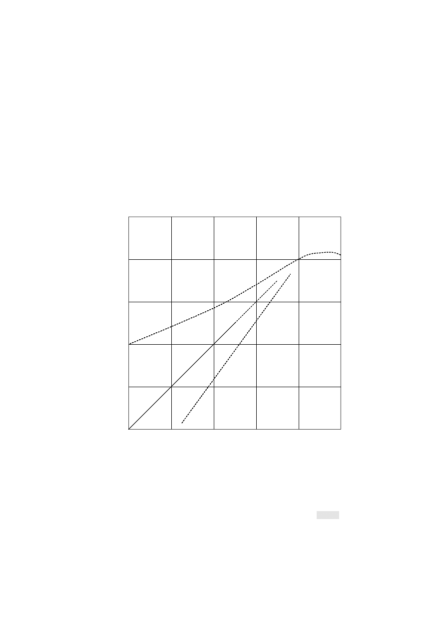
Recommendation ITU-R P.526. These upper and lower limits for the diffraction loss are shown in Fig. 1.
0530-01
40
30
20
10
0
–10
B
D
A
d
– 1.5
– 1
– 0.5
0
0.5
1
D
iff
ra
ct
io
n
lo
ss
re
la
ti
ve
t
o
f
ree
spa
ce (
d
B
)
Normalized clearance h/F
1
theoretical knife-edge loss curve
theoretical smooth spherical Earth loss curve, at 6.5 GHz and k = 4/3
empirical diffraction loss based on equation (2) for intermediate terrain
amount by which the radio path clears the Earth’s surface
radius of the first Fresnel zone
e
B:
D:
A :
h:
F :
d
1
FIGURE 1
Diffraction loss for obstructed line-of-sight
microwave radio paths
FIGURE 0539-01 = 3 CM
The diffraction loss over average terrain can be approximated for losses greater than about 15 dB by the formula:
A
d
=
– 20 h / F
1
+
10 dB
(2)

4
Rec. ITU-R P.530-7
where h is the height difference (m) between most significant path blockage and the path trajectory (h is negative if the
top of the obstruction of interest is above the virtual line-of-sight) and F
1
is the radius of the first Fresnel ellipsoid given
by:
F
d
d
f d
1
1
2
= 17.3
m
(3)
with:
f
:
frequency (GHz)
d
:
path length (km)
d
1
and d
2
:
distances (km) from the terminals to the path obstruction.
A curve, referred to as A
d
, based on equation (2) is also shown in Fig. 1. This curve, strictly valid for losses larger
than 15 dB, has been extrapolated up to 6 dB loss to fulfil the need of link designers.
2.2.2
Planning criteria for path clearance
At frequencies above about 2 GHz, diffraction fading of this type has in the past been alleviated by installing antennas
that are sufficiently high, so that the most severe ray bending would not place the receiver in the diffraction region when
the effective Earth radius is reduced below its normal value. Diffraction theory indicates that the direct path between the
transmitter and the receiver needs a clearance above ground of at least 60% of the radius of the first Fresnel zone to
achieve free-space propagation conditions. Recently, with more information on this mechanism and the statistics of k
e
that are required to make statistical predictions, some administrations are installing antennas at heights that will produce
some small known outage.
In the absence of a general procedure that would allow a predictable amount of diffraction loss for various small
percentages of time and therefore a statistical path clearance criterion, the following procedure is advised for temperate
and tropical climates.
2.2.2.1
Non-diversity antenna configurations
a)
determine the antenna heights required for the appropriate median value of the point k-factor (see § 2.2; in the
absence of any data, use k
=
4/3) and 1.0 F
1
clearance over the highest obstacle (temperate and tropical climates);
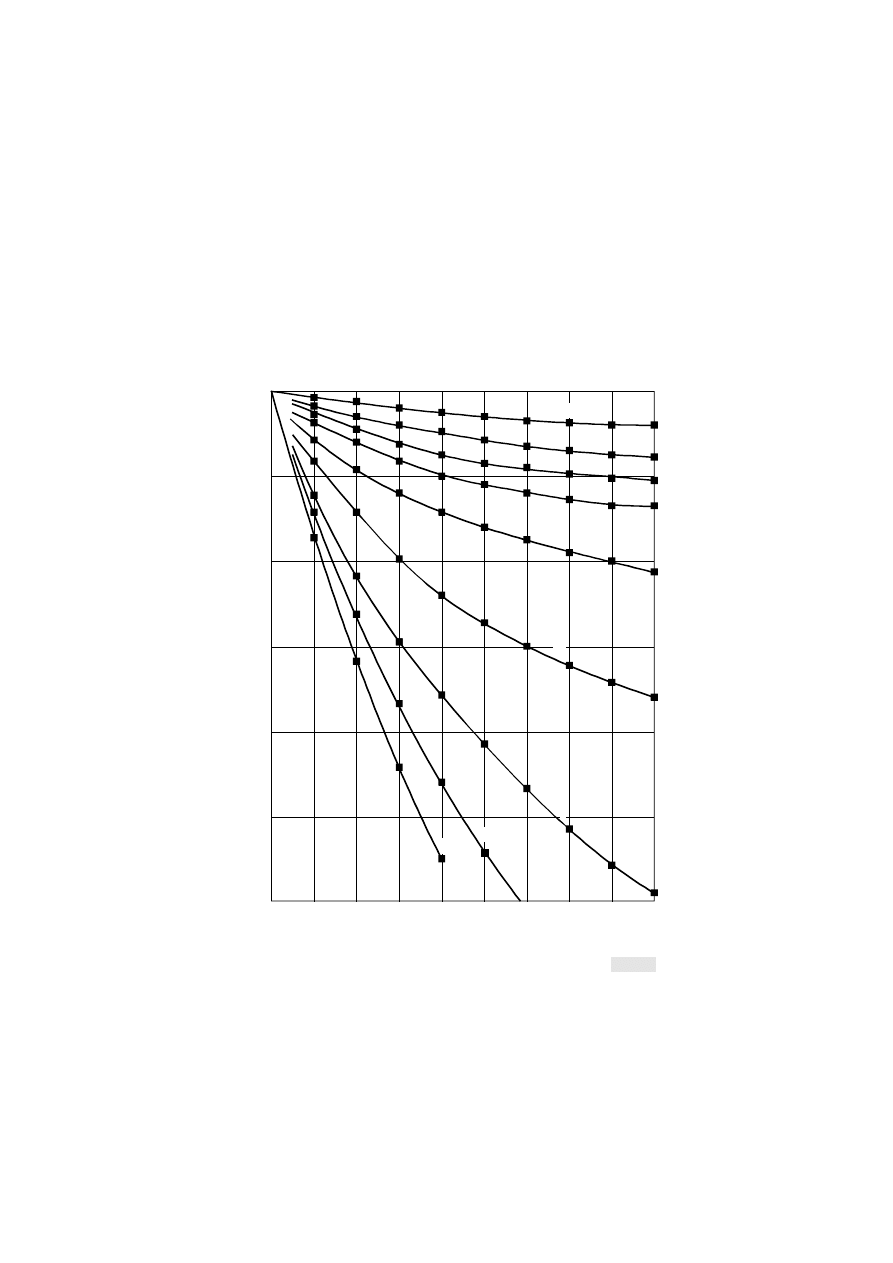
b)
obtain the value of k
e
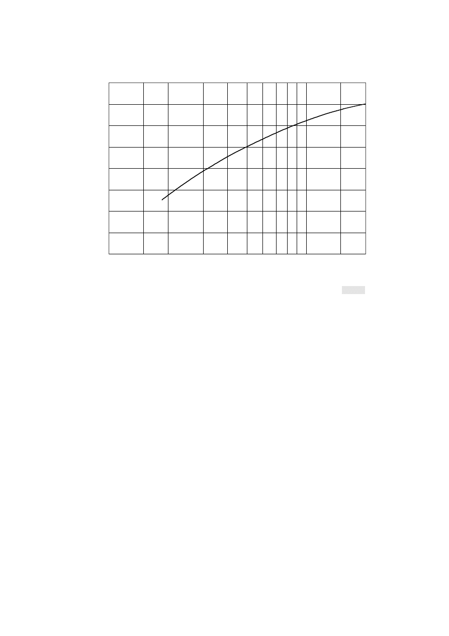
(99.9%) from Fig. 2 for the path length in question;
c)
calculate the antenna heights required for the value of k
e
obtained from step b) and the following Fresnel zone
clearance radii:
d)
use the larger of the antenna heights obtained by steps a) and c).
In cases of uncertainty as to the type of climate, the more conservative clearance rule for tropical climates may be
followed or at least a rule based on an average of the clearances for temperate and tropical climates. Smaller fractions
of F
1
may be necessary in steps a) and c) above for frequencies less than about 2 GHz in order to avoid unacceptably
large antenna heights.
Higher fractions of F
1
may be necessary in step c) for frequencies greater than about 10 GHz in order to reduce the risk
of diffraction in sub-refractive conditions.
Temperate climate
Tropical climate
0.0 F
1
(i.e. grazing) if there is a single isolated path obstruction
0.6 F
1
for path lengths greater than about 30 km
0.3 F
1
if the path obstruction is extended along a portion of the
path
Rec. ITU-R P.530-7
5
0530-02
10
2
10
2
5
2
1.1
1
0.9
0.8
0.7
0.6
0.5
0.4
0.3
Path length (km)
k
e
FIGURE 2
Value of k exceeded for approximately 99.9% of the worst month
(Continental temperate climate)
e
FIGURE 0539-02 = 3 CM
2.2.2.2
Two antenna space-diversity configurations
a)
Calculate the height of the lower antenna for the appropriate median value of the point k-factor (in the absence
of any data use k
=
4/3) and the following Fresnel zone clearances:
0.6 F
1
to 0.3 F
1
if the path obstruction is extended along a portion of the path;
0.3 F
1
to 0.0 F
1
if there are one or two isolated obstacles on the path profile.
One of the lower values in the two ranges noted above may be chosen if necessary to avoid increasing heights of existing
towers or if the frequency is less than 2 GHz.
Alternatively, the clearance of the lower antenna may be chosen to give about 6 dB of diffraction loss during normal
refractivity conditions (i.e. during the middle of the day), or some other loss appropriate to the fade margin of the
system, as determined by test measurements. Measurements should be carried out on several different days to avoid
anomalous refractivity conditions.
In this alternative case the diffraction loss can also be estimated using Fig. 1 or equation (2).
b)
Calculate the height of the upper antenna using the procedure for single antenna configurations noted above.
c)
Verify that the spacing of the two antennas satisfies the requirements for diversity under multipath fading
conditions. If not, increase the height of the upper antenna accordingly.
This fading, which results when the path is obstructed or partially obstructed by the terrain during sub-refractive
conditions, is the factor that governs antenna heights.
2.3
Fading and enhancement due to multipath and related mechanisms
Three clear-air fading mechanisms caused by extremely refractive layers in the atmosphere must be taken into account in
the planning of links of more than a few kilometres in length; beam spreading (commonly referred to as defocusing),
antenna decoupling, surface multipath, and atmospheric multipath. Most of these mechanisms can occur by themselves

6
Rec. ITU-R P.530-7
or in combination with each other (see Note 1). A particularly severe form of frequency selective fading occurs when
beam spreading of the direct signal combines with a surface reflected signal to produce multipath fading. Scintillation
fading due to smaller scale turbulent irregularities in the atmosphere is always present with these mechanisms but at
frequencies below about 40 GHz its effect on the overall fading distribution is not significant.
NOTE 1 – Antenna decoupling governs the minimum beamwidth of the antennas that should be chosen.
A method for predicting the single-frequency (or narrow-band) fading distribution at large fade depths in the average
worst month in any part of the world is given in § 2.3.1. This method does not make use of the path profile and can be
used for initial planning, licensing, or design purposes. A second method in § 2.3.2 that is suitable for all fade depths
employs the method for large fade depths and an interpolation procedure for small fade depths.
A method for predicting signal enhancement is given in § 2.3.3. The method uses the fade depth predicted by the method
in § 2.3.1 as the only input parameter. Finally, a method for converting average worst month to average annual
distributions is given in § 2.3.4.
2.3.1
Method for small percentages of time
2.3.1.1
For the path location in question, estimate the geoclimatic factor K for the average worst month from fading
data for the geographic area of interest if these are available (see Appendix 1).
Inland links: If measured data for K are not available, K can be estimated for links in inland areas (see Note 1 for
definition of inland links) from the following empirical relation in the climatic variable p
L
(i.e., the percentage of time
that the refractivity gradient in the lowest 100 m of the atmosphere is more negative than –100 N units/km in the
estimated average worst month; see below):
K
=
5.0
×
10
–7
×
10
–
0.1(C
0
– C
Lat
– C
Lon
)
p
L
1.5
(4)
The value of the coefficient C
0
in equation (4) is given in Table 1 for three ranges of altitude of the lower of the
transmitting and receiving antennas and three types of terrain (plains, hills, or mountains). In cases of uncertainty as to
whether a link should be classified as being in a plains or hilly area, the mean value of the coefficients C
0
for these two
types of area should be employed. Similarly, in cases of uncertainty as to whether a link should be classified as being in
a hilly or mountainous area, the mean value of the coefficients C
0
for these two types of area should be employed. Links
traversing plains at one end and mountains at the other should be classified as being in hilly areas. For the purposes of
deciding whether a partially overwater path is in a largely plains, hilly, or mountainous area, the water surface should be
considered as a plain.
For planning purposes where the type of terrain is not known, the following values of the coefficient C
0
in equation (4)
should be employed:
C
0
=
1.7
for lower-altitude antenna in the range 0-400 m above mean sea level;
C
0
=
4.2
for lower-altitude antenna in the range 400-700 m above mean sea level;
C
0
=
8
for lower-altitude antenna more than 700 m above mean sea level.
The coefficient C
Lat
in equation (4) of latitude
ξ
is given by:
C
Lat
=
0
(dB)
for
ξ
≤
53
°
N or
°
S
(5)
C
La
t
=
–53
+
ξ
(dB)
for 53
°
N or
°
S
<
ξ
<
60
°
N or
°
S
(6)
C
Lat
=
7
(dB)
for
ξ
≥
60
°
N or
°
S
(7)
and the longitude coefficient C
Lon
, by:
C
Lon
=
3
(dB)
for longitudes of Europe and Africa
(8)
C
Lon
=
–3
(dB)
for longitudes of North and South America
(9)
C
Lon
=
0
(dB)
for all other longitudes
(10)

Rec. ITU-R P.530-7
7
TABLE 1
Values of coefficient C
0
in equations (4) and (13) for three ranges
of lower antenna altitude and three types of terrain
The value of the climatic variable pL in equation (4) is estimated by taking the highest value of the –100 N units/km
gradient exceedance from the maps for the four seasonally representative months of February, May, August and
November given in Figs. 7-10 of Recommendation ITU-R P.453. An exception to this is that only the maps for May and
August should be used for latitudes greater than 60° N or 60° S.
It may be desirable in some cases to obtain expansions of the maps in Figs. 7-10 of Recommendation ITU-R P.453 in the
area of the link in question and accurately plot the point corresponding to the centre of the link to obtain the pL value.
Since the maps are on a Mercator projection, the following relation should be employed to accurately plot the centre
point latitude
ξ
:
(
)
[
]
(
)
[
]
(
)
[
]
(
)
[
]
∆
∆
z
z
L
=
tan
tan
tan
tan
1
2
1
ln
.
ln
.
ln
.
ln
.
45
0 5
45
0 5
45
0 5
45
0 5
° +
−
° +
° +
−
° +
ξ
ξ
ξ
ξ
(11)
Here
∆
z is the distance (e.g. in mm) between the nearest lower and upper latitude grid lines at latitudes
ξ
1
and
ξ
2
,
respectively (e.g. 30° and 45°);
∆
z
L
is the required distance (e.g. in mm) between the lower latitude grid line and the
point corresponding to the centre of the link. The centre point longitude can be plotted by linear interpolation.
Coastal links over/near large bodies of water: if measured data for K are not available for coastal links (see Note 2 for
definition) over/near large bodies of water (see Note 3 for definition of large bodies of water), K can be estimated from:
K
=
K
r
K
K
K
K
K
l
c
r
K
r
K
cl
i
i
cl
i
c
i
c
cl
( )
(
–
) log
log
=
≥
<
+
10
1
for
for
(12)
Altitude of lower antenna and type of link terrain
C
0
(dB)
Low altitude antenna (0-400 m) – Plains:
Overland or partially overland links, with lower-antenna altitude less than 400 m above mean sea level, located in largely
plains areas
0
Low altitude antenna (0-400 m) – Hills:
Overland or partially overland links, with lower-antenna altitude less than 400 m above mean sea level, located in largely
hilly areas
3.5
Medium altitude antenna (400-700 m) – Plains:
Overland or partially overland links, with lower-antenna altitude in the range 400-700 m above mean sea level, located
in largely plains areas
2.5
Medium altitude antenna (400-700 m) – Hills:
Overland or partially overland links, with lower-antenna altitude in the range 400-700 m above mean sea level, located
in largely hilly areas
6
High altitude antenna (
>
700 m) – Plains:
Overland or partially overland links, with lower-antenna altitude more than 700 m above mean sea level, located in
largely plains areas
5.5
High altitude antenna (
>
700 m) – Hills:
Overland or partially overland links, with lower-antenna altitude more than 700 m above mean sea level, located in
largely hilly areas
8
High altitude antenna (
>
700 m) – Mountains:
Overland or partially overland links, with lower-antenna altitude more than 700 m above mean sea level, located in
largely mountainous areas
10.5

8
Rec. ITU-R P.530-7
where r
c
is the fraction of the path profile below 100 m altitude above the mean level of the body of water in question
and within 50 km of the coastline, but without an intervening height of land above 100 m altitude, K
i
is given by the
expression for K in equation (4), and:
K
cl
=
2.3
×
10
–
4
×
10
–
0.1C
0
– 0.011 |
ξ
|
(13)
with C
0
given in Table 1. Note that the condition K
cl
<
K
i
in equation (12) occurs in a few regions at low and mid
latitudes.
Coastal links over/near medium-sized bodies of water: if measured data for K are not available for coastal links (see
Note 2 for definition) over/near medium-sized bodies of water (see Note 3 for definition of medium-sized bodies of
water), K can be estimated from:
K
=
K
r
K
K
K
K
K
m
c
r
K
r
K
cm
i
i
cm
i
c
i
c
cm
( )
(
–
) log
log
=
≥
<
+
10
1
for
for
(14)
and:
K
cm
=
10
0.5
(log K
i
+
log K
cl
)
(15)
with K
cl
given by equation (13). Note that the condition K
cm
<
K
i
in equation (15) occurs in a few regions at low and mid
latitudes.
NOTE 1 – Inland links are those in which either the entire path profile is above 100 m altitude (with respect to mean sea
level) or beyond 50 km from the nearest coastline, or in which part or all of the path profile is below 100 m altitude for a
link entirely within 50 km of the coastline, but there is an intervening height of land higher than 100 m between this part
of the link and the coastline. Links passing over a river or a small lake should normally be classed as passing over land.
For links in a region of many lakes, see Note 4.
NOTE 2 – The link may be considered to be crossing a coastal area if a fraction r
c
of the path profile is less than 100 m
above the mean level of a medium-sized or large body of water and within 50 km of its coastline, and if there is no
height of land above the 100 m altitude (relative to the mean altitude of the body of water in question) between this
fraction of the path profile and the coastline.
NOTE 3 –
The size of a body of water can be chosen on the basis of several known examples: Medium-sized bodies of
water include the Bay of Fundy (east coast of Canada) and the Strait of Georgia (west coast of Canada), the Gulf of
Finland, and other bodies of water of similar size. Large bodies of water include the English Channel, the North Sea, the
larger reaches of the Baltic and Mediterranean Seas, Hudson Strait, and other bodies of water of similar size or larger. In
cases of uncertainty as to whether the size of body of water in question should be classed as medium or large, K should
be calculated from:
K
r
K
r
K
K
c
i
c
cm
cl
=
−
+
+
10
1
0 5
(
) log
.
(log
log
)
(16)
NOTE 4 – Regions (not otherwise in coastal areas) in which there are many lakes over a fairly large area are believed to
behave somewhat like coastal areas. The region of lakes in southern Finland provides the best known example. Until
such regions can be better defined, K should be calculated from:
K
r
K
r
K
c
i
c
cm
=
−
+
10
0 5 2
. [(
) log
log
]
(17)
2.3.1.2
From the antenna heights h
e
and h
r
(m above sea level or some other reference height), calculate the magnitude
of the path inclination
|
ε
p
|
(mrad) from:
ε
p
r
e
h
h
d
=
–
/
(18)
where d, is the path length (km).
2.3.1.3
Calculate the percentage of time p
w
that fade depth A (dB) is exceeded in the average worst month from:
p
w
=
K d
3.6
f
0.89
(
1
+
| |
ε
p
)
–1.4
×
10
–A / 10
%
(19)
where f is the frequency (GHz).

Rec. ITU-R P.530-7
9
For prediction of exceedance percentages for the average year instead of the average worst month, see § 2.3.4.
NOTE 1 – Equation (19) was derived from fading data on paths with lengths in the range 7-95 km, frequencies in the
range 2-37 GHz, path inclinations for the range 0-24 mrad, and grazing angles in the range 1-12 mrad. Checks using
several other sets of data for paths up to 237 km in length and frequencies as low as 500 MHz suggest, however, that it is
valid for larger ranges of path length and frequency. The results of a semi-empirical analysis indicate that the lower
frequency limit of validity is inversely proportional to path length. A rough estimate of this lower frequency limit, ƒ
min
,
can be obtained from:
f
min
=
15 / d GHz
(20)
2.3.2
Method for various percentages of time
The method given below for predicting fade depths at various percentages of time combines an empirical interpolation
procedure between the deep fading region of the distribution and 0 dB, with the method given in the preceding section.
a)
Using the method in § 2.3.1, calculate the percentage of time p
w
that a fade depth of 35 dB is exceeded in the
tail of the distribution (i.e., equation (19)).
b)
Calculate the value of q
′
a
for the fade depth A
=
35 dB with the corresponding value of p
w
from step a):
q
′
a
=
–
20 log
10
– ln
100 – p
w
100
/
A
(21)
c)
Calculate the value of the parameter q
t
from:
q
t
=
(q
′
a
– 2)
/
1
+
0.3
×
10
–A / 20
10
–0.016 A
– 4.3
1
0
–A / 20
+
A /
8
00
(22)
d)
If q
t
>
0, repeat steps a) to c) for A
=
25 dB to obtain the definitive value of q
t
.
e)
For A
>
25 dB or A
>
35 dB, as appropriate, calculate the percentage of time p
w
that the fade depth A is
exceeded using the method in § 2.3.1. For A
<
25 dB, or A
<
35 dB, as appropriate, calculate the percentage of time p
w
that A is exceeded from:
p
w
=
100
1 – exp
–10
–q
a
A / 20
%
(23)
where q
a
is also a function of A given by:
q
a
=
2
+
1
+
0.3
×
10
–A / 20
10
–
0.016 A
q
t
+
4.3
10
–A / 20
+
A / 800
(24)
Here the value of parameter q
t
is that obtained in step c) or d) as appropriate. With q
t
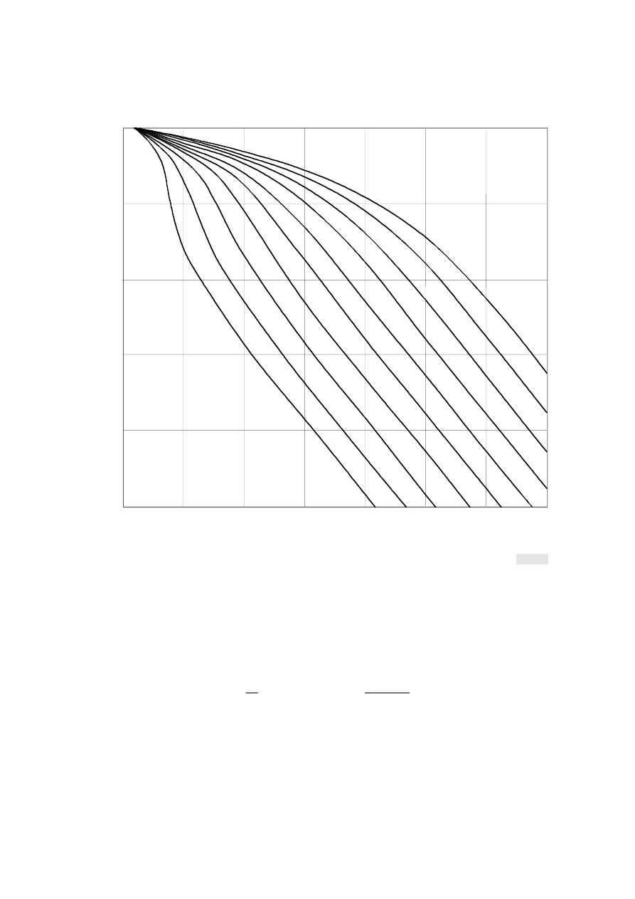
as a parameter, Fig. 3 gives a
family of curves providing a graphical representation of the method.
For prediction of exceedance percentages for the average year instead of the average worst month, see § 2.3.4.
2.3.3
Prediction method for enhancement
Large enhancements are observed during the same general conditions of frequent ducts that result in multipath fading.
Average worst month enhancement above 10 dB should be predicted using:
p
w
=
100 – 10
(–1.7
+
0.2 A
0.01
– E
) / 3.5
% for E > 10 dB
(25)
where E is the enhancement (dB) not exceeded for p% of the time and A
0.01
is the predicted deep fade depth using
equation (19) exceeded for p
w
=
0.01% of the time.
10
Rec. ITU-R P.530-7
0530-03
0
10
20
30
40
50
t
q = 7
6
5
4
3
2
1
0
–1
10
10
10
10
10
10
10
2
–1
–2
–3
–4
–5
1
t
q = –2
Fa
de de
pt
h
,
A
(dB
)
Percentage of time, p
w
FIGURE 3
Percentage of the time fade depth exceeded in an average
worst month, with q
t
(in equation (24)) ranging from –2 to 7
FIGURE 0530-03 = 3 CM
For the enhancement between 10 and 0 dB use the following step-by-step procedure:
a)
Calculate the percentage of time p
′
w
with enhancement less or equal to 10 dB (E
′
=
10) using equation (25).
b)
Calculate q
′
e
using:
q
′
e
=
–
20
E
′
log
10
– ln
1 –
100 – p
′
w
58.21
(26)
c)
Calculate the parameter q
s
from:
q
s
=
2.05 q
′
e
– 20.3
(27)
d)
Calculate q
e
for the desired E using:
q
e
=
8
+
1
+
0.3
×
10
–E / 20
10
–0.7
E / 20
q
s
+
12
10
–E / 20
+
E / 800
(28)
Rec. ITU-R P.530-7
11
e)
The percentage of time that the enhancement E (dB) is not exceeded is found from:
p
w
=
100 – 58.21
1 – exp
–10–
q
e
E / 20
(29)
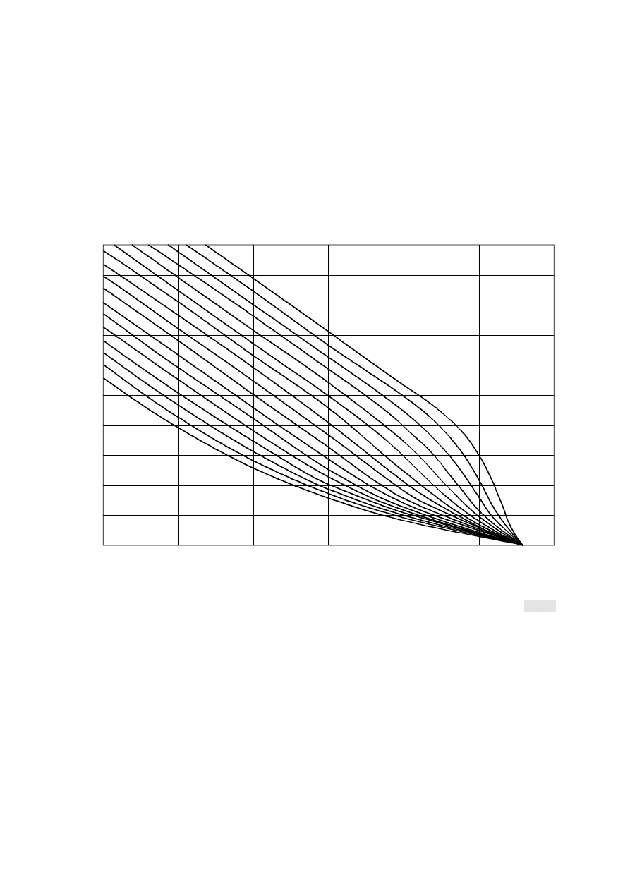
The set of curves in Fig. 4 with q
s
as a parameter gives a graphical representation of the method.
0530-04
q = 2
s
q = –14
s
10
10
10
10
10
10
1
–4
–3
–2
–1
2
0
2
4
6
8
10
12
14
16
18
20
Enh
a
nc
emen
t,
E
(dB
)
Percentage of time (100 – p )
FIGURE 4
Prediction of enhancement for various percentages of time,
with q
s
(in equation (28)) ranging from –14 to 2
w
FIGURE 0539-04 = 3 CM
For prediction of exceedance percentages for the average year instead of the average worst month, see § 2.3.4.
2.3.4
Conversion from average worst month to average annual distributions
The fading and enhancement distributions for the average worst month obtained from the methods of § 2.3.1-2.3.3 can
be converted to distributions for the average year by employing the following procedure:
a)
Calculate the percentage of time p
w
fade depth A is exceeded in the large tail of the distribution for the average
worst month from equation (19).
b)
Calculate the logarithmic geoclimatic conversion factor
∆
G from:
∆
G
=
10.5 – 5.6 log (1.1
±
|cos 2
ξ
|
0.7
) – 2.7 log d
+
1.7 log (1
+
|
ε
p
|) dB
(30)

12
Rec. ITU-R P.530-7
where
∆
G
≤
10.8 dB and the positive sign in equation (30) is employed for
ξ
≤
45° and the negative sign for
ξ
>
45°,
and where:
ξ
:
latitude (
°
N or
°
S)
d
:
path length (km)
|
ε
p
|
:
magnitude of path inclination (obtained from equation (18)).
c)
Calculate the percentage of time p fade depth A is exceeded in the large fade depth tail of the distribution for
the average year from:
p
=
10
–
∆
G
/
10
p
w
%
(31)
d)
If the shallow fading range of the distribution is required (i.e. A
<
25 dB or A
<
35 dB, as appropriate) follow
the method of § 2.3.2, replacing p
w
by p.
e)
If it is required to predict the distribution of enhancement for the average year, follow the method of § 2.3.3,
where A
0.01
is now the fade depth exceeded for 0.01% of the time in the average year. Obtain first p
w
by inverting
equation (31) and using p
=
0.01%. Then obtain fade depth A
0.01
exceeded for 0.01% of the time in the average year by
inverting equation (19) and using p in place of p
w
.
2.3.5
Prediction of non-selective outage (see Note 1)
In the design of a digital link, calculate the probability of outage P
ns
due to the non-selective component of the fading
(see § 7) from:
P
p
ns
w
=
/ 100
(32)
where p
w
(%) is the percentage of time that the flat fade margin A
=
F (dB) corresponding to the specified bit error ratio
(BER) is exceeded in the average worst month (obtained from § 2.3.1 or § 2.3.2, as appropriate). The flat fade margin, F,
is obtained from the link calculation and the information supplied with the particular equipment, also taking into account
possible reductions due to interference in the actual link design.
NOTE 1 – The outage is calculated for a certain BER that corresponds to a severely-errored-second (SES) event (see § 7
for further information).
2.3.6
Occurrence of simultaneous fading on multi-hop links
Experimental evidence indicates that, in clear-air conditions, fading events exceeding 20 dB on adjacent hops in a multi-
hop link are almost completely uncorrelated. This suggests that, for analogue systems with large fade margins, the
outage time for a series of hops in tandem is approximately given by the sum of the outage times for the individual hops.
For fade depths not exceeding 10 dB, the probability of simultaneously exceeding a given fade depth on two adjacent
hops can be estimated from:
P
12
=
(P
1
P
2
)
0.8
(33)
where P
1
and P
2
are the probabilities of exceeding this fade depth on each individual hop (see Note 1).
The correlation between fading on adjacent hops decreases with increasing fade depth between 10 and 20 dB, so that the
probability of simultaneously exceeding a fade depth greater than 20 dB can be approximately expressed by:
P
12
=
P
1
P
2
(34)
NOTE 1 – The correlation between fading on adjacent hops is expected to be dependent on path length. Equation (33) is
an average based on the results of measurements on 47 pairs of adjacent line-of-sight hops operating in the 5 GHz band,
with path lengths in the range 11-97 km, and an average path length of approximately 45 km.

Rec. ITU-R P.530-7
13
2.4
Attenuation due to hydrometeors
Attenuation can also occur as a result of absorption and scattering by such hydrometeors as rain, snow, hail and fog.
Although rain attenuation can be ignored at frequencies below about 5 GHz, it must be included in design calculations at
higher frequencies, where its importance increases rapidly. A technique for estimating long-term statistics of rain
attenuation is given in § 2.4.1. On paths at high latitudes or high altitude paths at lower latitudes, wet snow can cause
significant attenuation over an even larger range of frequencies. More detailed information on attenuation due to
hydrometeors other than rain is given in Recommendation ITU-R P.840.
At frequencies where both rain attenuation and multipath fading must be taken into account, the exceedance percentages
for a given fade depth corresponding to each of these mechanisms can be added.
2.4.1
Long-term statistics of rain attenuation
The following simple technique may be used for estimating the long-term statistics of rain attenuation:
Step 1:
Obtain the rain rate R
0.01
exceeded for 0.01% of the time (with an integration time of 1 min). If this
information is not available from local sources of long-term measurements, an estimate can be obtained from the
information given in Recommendation ITU-R P.837.
Step 2:
Compute the specific attenuation,
γ
R
(dB/km) for the frequency, polarization and rain rate of interest using
Recommendation ITU-R P.838.
Step 3:
Compute the effective path length d
eff
of the link by multiplying the actual path length d by a distance factor r.
An estimate of this factor is given by:
r
=
1
1
+
d / d
0
(35)
where, for R
0.01
≤
100 mm/h:
d
0
=
35 e
–
0.015 R
0.01
(36)
For R
0.01
>
100 mm/h, use the value 100 mm/h in place of R
0.01
.
Step 4:
An estimate of the path attenuation exceeded for 0.01% of the time is given by:
A
0.01
=
γ
R
d
eff
=
γ
R
dr dB
(37)
Step 5:
Attenuation exceeded for other percentages of time p in the range 0.001% to 1% may be deduced from the
following power law:
A
p
A
0.01
=
0.12 p
–
(0.546
+
0.043 log
10
p)
(38)
This formula has been determined to give factors of 0.12, 0.39, 1 and 2.14 for 1%, 0.1%, 0.01% and 0.001%
respectively, and must be used only within this range.
Step 6:
If worst-month statistics are desired, calculate the annual time percentages p corresponding to the worst-month
time percentages p
w
using climate information specified in Recommendation ITU-R P.841. The values of A exceeded for
percentages of the time p on an annual basis will be exceeded for the corresponding percentages of time p
w
on a worst-
month basis.
The prediction procedure outlined above is considered to be valid in all parts of the world at least for frequencies up to
40 GHz and path lengths up to 60 km.
2.4.2
Frequency scaling of long-term statistics of rain attenuation
When reliable long-term attenuation statistics are available at one frequency the following empirical expression may be
used to obtain a rough estimate of the attenuation statistics for other frequencies in the range 7 to 50 GHz, for the same
hop length and in the same climatic region:
A
2
=
A
1
(
Φ
2
/
Φ
1
)
1 – H(
Φ
1
,
Φ
2
, A
1
)
(39)

14
Rec. ITU-R P.530-7
where:
Φ
(
f
)
=
f
2
1
+
10
–
4
f
2
(40)
H
(
Φ
1
,
Φ
2
, A
1
)
=
1.12
×
10
–3
(
Φ
2
/
Φ
1
)
0.5
(
Φ
1
A
1
)
0.55
(41)
Here, A
1
and A
2
are the equiprobable values of the excess rain attenuation at frequencies f
1
and f
2
(GHz), respectively.
2.4.3
Polarization scaling of long-term statistics of rain attenuation
Where long-term attenuation statistics exist at one polarization (either vertical or horizontal) on a given link, the
attenuation for the other polarization over the same link may be estimated through the following simple formulae:
A
V
=
300 A
H
335
+
A
H
dB
(42)
or:
A
H
=
335 A
V
300 – A
V
dB
(43)
These expressions are considered to be valid in the range of path length and frequency for the prediction method
of § 2.4.1.
2.4.4
Statistics of duration and fading
There is some evidence that the rate of fading due to rain is much less than that due to multipath. On the other hand, the
average and median values of duration differ, indicating skewness of the distribution of fading duration.
2.4.5
Tandem and convergent paths, and path diversity
2.4.5.1
Length of individual hops
The overall transmission performance of a tandem system is largely influenced by the propagation characteristics of the
individual links. It is sometimes possible to achieve the same overall physical connection by different combinations of
hop lengths. Increasing the length of individual hops inevitably results in an increase in the probability of outage for
those hops. On the other hand, such a move could mean that fewer hops might be required and the overall performance
of the tandem system might not be impaired.
2.4.5.2
Correlated fading on tandem paths
If the occurrence of rainfall were statistically independent of location, then the overall probability of fading for a linear
series of links in tandem would be given to a good approximation by:
P
T
=
∑
i
=
1
n
P
i
(44)
where P
i
is the ith of the total n links.
On the other hand, if precipitation events are correlated over a finite area, then the attenuation on two or more links of a
multi-hop relay system will also be correlated, in which case the combined fading probability may be written as:
P
T
=
K
∑
i
=
1
n
P
i
(45)
where K is a modification factor that includes the overall effect of rainfall correlation.
Rec. ITU-R P.530-7
15
Few studies have been conducted with regard to this question. One such study examined the instantaneous correlation of
rainfall at locations along an East-West route, roughly parallel to the prevailing direction of storm movement. Another
monitored attenuation on a series of short hops oriented North-South, or roughly perpendicular to the prevailing storm
track during the season of maximum rainfall.
For the case of links parallel to the direction of storm motion, the effects of correlation for a series of links each more
than 40 km in length, l, were slight. The modification factor, K, in this case exceeded 0.9 for rain induced outage
of 0.03% and may reasonably be ignored (see Fig. 5). For shorter hops, however, the effects become more significant:
the overall outage probability for 10 links of 20, 10 and 5 km each is approximately 80%, 65% and 40% of the
uncorrelated expectation, respectively (modification factors 0.8, 0.65, 0.4). The influence of rainfall correlation is seen
to be somewhat greater for the first few hops and then decreases as the overall length of the chain increases.
0530-05
1
2
3
4
5
6
7
8
9
10
L
= 80 km
50
40
30
20
10
5
3
2
0.4
0.5
0.6
0.7
0.8
0.9
1.0
M
odi
fi
ca
ti
on
f
a
ct
o
r,
K
Number of hops
FIGURE 5
Modification factor for joint rain attenuation on a series of tandem links
of equal length,
L
, for an exceedance probability of 0.03% for each link
FIGURE 0539-05 = 3 CM
16
Rec. ITU-R P.530-7
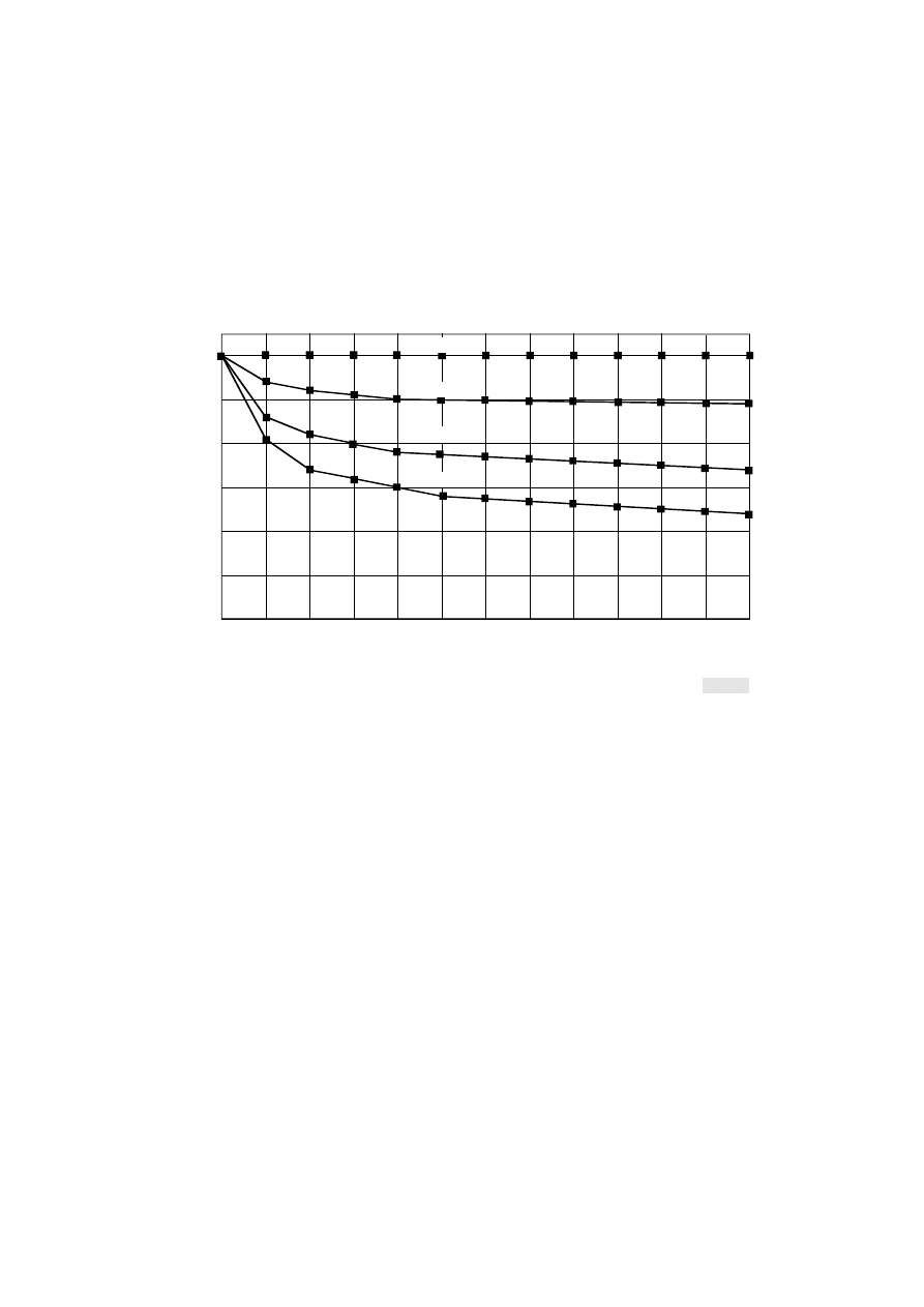
The modification factors for the case of propagation in a direction perpendicular to the prevailing direction of storm
motion are shown in Fig. 6 for several probability levels. In this situation, the modification factors fall more rapidly for
the first few hops (indicating a stronger short-range correlation than for propagation parallel to storm motion) and
maintain relatively steady values thereafter (indicating a weaker long-range correlation).
0530-06
2
3
4
5
6
7
8
9
10
11
12
13
1
M
odi
fi
ca
ti
on
f
a
ct
o
r,
K
Number of relay links
(May 1975-March 1979)
FIGURE 6
Modification factor for joint rain attenuation on a series
of tandem links of approximately 4.6 km each for several exceedance
probability levels for each link
0.8
0.7
0.6
0.5
0.4
0.9
1.0
0.0001%
0.001%
0.01%
0.1%
FIGURE 0539-06 = 3 CM
2.4.5.3
Convergent paths
Where two or more radio paths converge to one radio-relay station, the correlation coefficient of attenuation between
pairs of paths is dependent on the angle between the paths. This dependence, together with the differential attenuation on
the converging paths and the interference between paths, was studied for the case when the path length is smaller or
comparable in size with the rain cell. As an example it was found theoretically that for a path length of 4 km, the
correlation coefficient increased from 0.8 to 0.97 when the angle between the paths decreased from 180° to 20°.
2.4.5.4
Path diversity
Whereas fading due to multipath propagation can be overcome by a vertical separation of several metres between the
antennas, a choice of paths with a separation of several kilometres may reduce fading due to precipitation.
Experimental data obtained in the United Kingdom in the 20-40 GHz range give an indication of the improvement in
link reliability which can be obtained by the use of switched-path route diversity. The diversity gain (i.e. the difference
between the attenuation (dB) exceeded for a specific percentage of time on a single link and that simultaneously on two
parallel links):
–
tends to decrease as the path length increases from 12 km for a given percentage of time, and for a given lateral path
separation,
–
is generally greater for a spacing of 8 km than for 4 km, though an increase to 12 km does not provide further
improvement,
–
is not significantly dependent on frequency in the range 20-40 GHz, for a given geometry, and
–
ranges from about 2.8 dB at 0.1% of the time to 4.0 dB at 0.001% of the time, for a spacing of 8 km, and path
lengths of about the same value. Values for a 4 km spacing are about 1.8 to 2.0 dB.

Rec. ITU-R P.530-7
17
2.4.6
Prediction of outage due to precipitation
In the design of a digital link, calculate the probability P
rain
of exceeding a rain attenuation equal to the flat fade margin
F (dB) (see § 2.3.5) for the specified BER from:
P
p
rain
=
/ 100
(46)
where p (%) is the percentage of time that a rain attenuation of F (dB) is exceeded in the average year by solving
equation (38) in § 2.4.1.
3
Variation in angle-of-arrival/launch
Abnormal gradients of the clear-air refractive index along a path can cause considerable variation in the angles of launch
and arrival of the transmitted and received waves. This variation is substantially frequency independent and primarily in
the vertical plane of the antennas. The range of angles is greater in humid coastal regions than in dry inland areas. No
significant variations have been observed during precipitation conditions.
The effect can be important on long paths in which high gain/narrow beam antennas are employed. If the antenna
beamwidths are too narrow, the direct outgoing/incoming wave can be sufficiently far off axis that a significant fade can
occur (see § 2.3). Furthermore, if antennas are aligned during periods of very abnormal angles-of-arrival, the alignment
may not be optimum. Thus, in aligning antennas on critical paths (e.g. long paths in coastal area), it may be desirable to
check the alignment several times over a period of a few days.
4
Reduction of cross-polarization discrimination
The cross-polarization discrimination (XPD) can deteriorate sufficiently to cause co-channel interference and, to a lesser
extent, adjacent channel interference. The reduction in XPD that occurs during both clear-air and precipitation
conditions must be taken into account.
4.1
Prediction of outage due to clear-air effects
The combined effect of multipath propagation and the cross-polarization patterns of the antennas governs the reductions
in XPD occurring for small percentages of time. To compute the effect of these reductions in link performance the
following step-by-step procedures should be used:
Step 1:
Compute
XPD
XPD
XPD
XPD
g
g
g
0
5
35
40
35
=
+
≤
>
for
for
(47)
where XPD
g
is the manufacturer’s guaranteed minimum XPD at boresight for both the transmitting and receiving
antennas, i.e., the minimum of the transmitting and receiving antenna boresight XPDs.
Step 2:
Evaluate the multipath activity parameter
( )
η =
−
−
1
0 2
0
0 75
e
.
.
P
(48)
where P
0
=
p
w
/100 is the multipath occurrence factor corresponding to the percentage of the time p
w
(%) of exceeding
A
=
0 dB in the average worst month, as calculated from equation (19).
Step 3:
Determine
Q
k
P
xp
= −
10
0
log
η
(49)

18
Rec. ITU-R P.530-7
where:
k
s
xp
t
=
−
−
×
−
0 7
1
0 3
4
10
6
2
.
. exp
one transmit antenna
two transmit antennas
λ
(50)
In the case where two orthogonally polarized transmissions are from different antennas, the vertical separation is s
t
(m)
and the carrier wavelength is
λ
(m).
Step 4:
Derive the parameter C from:
C
XPD
Q
=
+
0
(51)
Step 5:
Calculate the probability of outage P
xp
due to clear-air cross-polarization from:
P
P
xp
M
XPD
=
×
−
0
10
10
(52)
where M
XPD
(dB) is the equivalent XPD margin for a reference BER given by:
M
C
C
I
C
C
I
XPIF
XPD
=
−
−
+
0
0
without XPIC
with XPIC
(53)
Here, C
0
/I is the carrier-to-interference ratio for a reference BER, which can be evaluated either from simulations or
from measurements.
XPIF is a laboratory-measured cross-polarization improvement factor that gives the difference in cross-polar isolation
XPI at sufficiently large carrier-to-noise ratio (typically 35 dB) and at a specific BER for systems with and without cross
polar interference canceller (XPIC). A typical value of XPIF is about 20 dB.
4.2
Prediction of outage due to precipitation effects
4.2.1
XPD statistics during precipitation conditions
Intense rain governs the reductions in XPD observed for small percentages of time. For paths on which more detailed
predictions or measurements are not available, a rough estimate of the unconditional distribution of XPD can be obtained
from a cumulative distribution of the co-polarized rain attenuation CPA (see § 2.4) using the equi-probability relation:
XPD
=
U – V(
f
) log CPA dB
(54)
that applies for both linear and circular polarizations. The coefficients U and V(
f
) are in general dependent on a number
of variables and empirical parameters, including frequency, f
. For line-of-sight paths with small elevation angles and
horizontal or vertical polarization, these coefficients may be approximated by:
U
=
U
0
+
30 log f
(55)
V
(
f
)
=
12.8 f
0.19
for
8
≤
f
≤
20 GHz
V
(
f
)
=
22.6
for 20 < f
≤
35 GHz
(56)
An average value of U
0
of about 15 dB, with a lower bound of 9 dB for all measurements, has been obtained for
attenuations greater than 15 dB.
The variability in the values of U and V(
f
) is such that the difference between the CPA values for vertical and horizontal
polarizations is not significant when evaluating XPD. The user is advised to use the value of CPA for circular
polarization when working with equation (54).

Rec. ITU-R P.530-7
19
Long-term XPD statistics obtained at one frequency can be scaled to another frequency using the semi-empirical
formula:
XPD
2
=
XPD
1
– 20 log (
f
2
/
f
1
) for 4
≤
f
1
, f
2
≤
30 GHz
(57)
where XPD
1
and XPD
2
are the XPD values not exceeded for the same percentage of time at frequencies f
1
and f
2
.
The relationship between XPD and CPA is influenced by many factors, including the residual antenna XPD, that has not
been taken into account. Equation (57) is least accurate for large differences between the respective frequencies. It is
most accurate if XPD
1
and XPD
2
correspond to the same polarization (horizontal or vertical).
4.2.2
Step-by-step procedure for predicting outage due to precipitation effects
Step 1:
Determine the path attenuation, A
0,01
(dB), exceeded for 0.01% of the time from equation (37).
Step 2:
Determine the equivalent path attenuation, A
p
(dB):
A
p
U
C I
XPIF
V
=
−
+
10
0
((
/
) /
)
(58)
where U is obtained from equation (55) and V from equation (56), C
0
/I (dB) is the carrier-to-interference ratio defined
for the reference BER without XPIC, and XPIF (dB) is the cross-polarized improvement factor for the reference BER.
If an XPIC device is not used, set XPIF
=
0.
Step 3:
Determine the following parameters:
[
]
m
A
A
m
p
=
≤
23 26
0 12
40
40
0 01
.
log
.
.
if
otherwise
(59)
and:
(
)
n
m
= −
+
−
12 7
161 23
4
2
.
.
/
(60)
Valid values for n must be in the range of –3 to 0. Note that in some cases, especially when an XPIC device is used,
values of n less than –3 may be obtained. If this is the case, it should be noted that values of p less than –3 will give
outage BER < 1
×
10
–5
.
Step 4:
Determine the outage probability from:
P
XPR
n
=
−
10
2
(
)
(61)
5
Distortion due to propagation effects
The primary cause of distortion on line-of-sight links in the UHF and SHF bands is the frequency dependence of
amplitude and group delay during clear-air multipath conditions. In analogue systems, an increase in fade margin will
improve the performance since the impact of thermal noise is reduced. In digital systems, however, the use of a larger
fade margin will not help if it is the frequency selective fading that causes the performance reduction.
The propagation channel is most often modelled by assuming that the signal follows several paths, or rays, from the
transmitter to the receiver. These involve the direct path through the atmosphere and may include one or more additional
ground-reflected and/or atmospheric refracted paths. If the direct signal and a significantly delayed replica of near equal
amplitude reach the receiver, inter symbol interference occurs that may result in an error in detecting the information.
Performance prediction methods make use of such a multi-ray model by integrating the various variables such as delay
(time difference between the first arrived ray and the others) and amplitude distributions along with a proper model of

20
Rec. ITU-R P.530-7
equipment elements such as modulators, equaliser, forward-error correction (FEC) schemes, etc. Although many
methods exist, they can be grouped into three general classes based on the use of a system signature, linear amplitude
distortion (LAD), or net fade margin. The signature approach often makes use of a laboratory two-ray simulator model,
and connects this to other information such as multipath occurrence and link characteristics. The LAD approach
estimates the distortion distribution on a given path that would be observed at two frequencies in the radio band and
makes use of modulator and equaliser characteristics, etc. Similarly, the net-fade margin approach employs estimated
statistical distributions of ray amplitudes as well as equipment information, much as in the LAD approach. In § 5.1, the
method recommended for predicting error performance is a signature method.
Distortion resulting from precipitation is believed to be negligible, and in any case a much less significant problem than
precipitation attenuation itself. Distortion is known to occur in millimetre and sub-millimetre wave absorption bands, but
its effect on operational systems is not yet clear.
5.1
Prediction of outage in unprotected digital systems
The outage probability is here defined as the probability that BER is larger than a given threshold.
Step 1:
Calculate the mean time delay from:
τ
m
d
=
0 7
50
1 3
.
.
ns
(62)
where d is the path length (km).
Step 2:
Calculate the multipath activity parameter
η
as in Step 2 of § 4.1.
Step 3:
Calculate the selective outage probability from:
P
W
W
s
M
B
m
r M
NM
B
m
r NM
M
NM
=
×
+
×
−
−
2 15
10
10
20
2
20
2
.
/
,
/
,
η
τ
τ
τ
τ
(63)
where:
W
x
: signature width (GHz)
B
x
:
signature depth (dB)
τ
r,x
: the reference delay (ns) used to obtain the signature, with x denoting either minimum phase (M) or non-
minimum phase (NM) fades.
The signature parameter definitions and specification of how to obtain the signature are given in Recommenda-
tion ITU-R F.1093.
6
Techniques for alleviating the effects of multipath propagation
The effects of slow relatively non-frequency selective fading (i.e. “flat fading”) due to beam spreading, and faster
frequency-selective fading due to multipath propagation can be reduced by both non-diversity and diversity techniques.
6.1
Techniques without diversity
Links should be sited to take advantage of terrain in ways that will increase the path inclination, since increasing path
inclination is known to reduce the effects of beam spreading, surface multipath fading, and atmospheric multipath
fading. Links should also be sited where possible to reduce the level of surface reflections thus reducing the occurrence
of multipath fading and distortion. Techniques include the siting of overwater links to place surface reflections on land
rather than water and the siting of overland and overwater links to similarly avoid large flat highly reflecting surfaces on
land. Another technique known to reduce the level of surface reflections is to tilt the antennas slightly upwards. Detailed

Rec. ITU-R P.530-7
21
information on appropriate tilt angles is not yet available. A trade-off must be made between the resultant loss in antenna
directivity in normal refractive conditions that this technique entails, and the improvement in multipath fading
conditions.
Another technique that is less well understood involves the reduction of path clearance. A trade-off must be made
between the reduction of the effects of multipath fading and distortion and the increased fading due to sub-refraction.
6.2
Diversity techniques
Diversity techniques include space, angle and frequency diversity. Frequency diversity should be avoided whenever
possible so as to conserve spectrum. Whenever space diversity is used, angle diversity should also be employed by
tilting the antennas at different upward angles. Angle diversity can be used in situations in which adequate space
diversity is not possible or to reduce tower heights.
The degree of improvement afforded by all of these techniques depends on the extent to which the signals in the
diversity branches of the system are uncorrelated. For narrow-band analogue systems, it is sufficient to determine the
improvement in the statistics of fade depth at a single frequency. For wideband digital systems, the diversity
improvement also depends on the statistics of in-band distortion.
The diversity improvement factor, I, for fade depth, A, is defined by:
I
=
p(
A
)
/
p
d
(
A
)
(64)
where p
d
(A) is the percentage of time in the combined diversity signal branch with fade depth larger than A and p(A) is
the percentage for the unprotected path. The diversity improvement factor for digital systems is defined by the ratio of
the exceedance times for a given BER with and without diversity. A prediction procedure for the diversity improvement
factor can be currently recommended only for narrow-band space-diversity systems.
6.2.1
Diversity techniques in analogue systems
The vertical space diversity improvement factor for narrow-band signals on an overland path can be estimated from:
I
=
1 – exp
–3.34
×
10
–
4
S
0.87
f
–
0.12
d
0.48
P
–1.04
0
10
(
A – V
) / 10
(65)
where:
P
0
=
p
w
⋅
10
A / 10
/
100
(66)
and:
V
=
G
1
– G
2
(67)
with:
A
:
fade depth (dB) for the unprotected path
p
w
:
percentage of time fade depth A is exceeded in the average worst month
P
0
:
fading occurrence factor
S
:
vertical separation (centre-to-centre) of receiving antennas (m)
f
:
frequency (GHz)
d
:
path length (km)
G
1
, G
2
:
gains of the two antennas (dBi).

22
Rec. ITU-R P.530-7
This equation was based on data in the data banks of Radiocommunication Study Group 3 for the following ranges of
variables: 43
≤
d
≤
240 km, 2
≤
f
≤
11 GHz, and 3
≤
S
≤
23 m. There is some reason to believe that it may remain
reasonably valid for path lengths as small as 25 km. The exceedance percentage p
w
can be calculated from equation (19).
Equation (65) is valid in the deep-fading range for which equation (19) is valid.
6.2.2
Diversity techniques in digital systems
Methods are available for predicting outage probability and diversity improvement for space, frequency, and angle
diversity systems, and for systems employing a combination of space and frequency diversity. The step-by-step
procedures are as follows.
6.2.2.1
Prediction of outage using space diversity
In space diversity systems, maximum-power combiners have been used most widely so far. The step-by-step procedure
given below applies to systems employing such a combiner. Other combiners, employing a more sophisticated approach
using both minimum-distortion and maximum-power dependent on a radio channel evaluation may give somewhat better
performance.
Step 1:
Calculate the multipath activity factor,
η
, as in Step 2 of § 4.1.
Step 2: Calculate the square of the non-selective correlation coefficient, k
ns
, from:
k
I
P
ns
ns
ns
2
1
=
−
⋅
η
(68)
where the improvement, I
ns
, can be evaluated from equation (65) for a fade depth A (dB) corresponding to the flat fade
margin F (dB) (see § 2.3.5) and P
ns
from equation (32).
Step 3:
Calculate the square of the selective correlation coefficient, k
s
, from:
(
)
(
)
k
r
r
r
r
r
s
w
w
r
w
w
w
w
2
0 109
0 13
1
0 5136
0 8238
0 5
1
0 195 1
0 5
0 9628
1
0 3957 1
0 9628
=
≤
−
−
<
≤
−
−
>
−
−
.
.
.
.
.
.
.
.
.
log (
)
.
for
for
for
(69)
where the correlation coefficient, r
w
, of the relative amplitudes is given by:
(
)
(
)
r
k
k
k
k
w
ns
ns
ns
ns
=
−
−
≤
−
−
>
1
0 9746 1
0 26
1
0 6921 1
0 26
2
2 170
2
2
1 034
2
.
.
.
.
.
.
for
for
(70)
Step 4:
Calculate the non-selective outage probability, P
dns
, from:
P
P
I
dns
ns
ns
=
(71)
where P
ns
is the non-protected outage given by equation (32).
Step 5:
Calculate the selective outage probability, P
ds
, from:
(
)
P
P
k
ds
s
s
=
−
2
2
1
η
(72)
where P
s
is the non-protected outage given by equation (63).
Step 6:
Calculate the total outage probability, P
d
, as follows:
(
)
P
P
P
d
ds
dns
=
+
0 75
0 75
1 33
.
.
.
(73)

Rec. ITU-R P.530-7
23
6.2.2.2
Prediction of outage using frequency diversity
The method given applies for a 1
+
1 system. Employ the same procedure as for space diversity, but in Step 2 use
instead:
I
fd
f
f
ns
F
=
80
10
10
∆
/
(74)
where:
∆
f
: frequency separation (GHz)
f
:
carrier frequency (GHz).
6.2.2.3
Prediction of outage using angle diversity
Step 1:
Estimate the average angle of arrival,
µθ
, from:
µ
θ
=
×
−
2 89
10
5
.
G
d
m
degrees
(75)
where G
m
is the average value of the refractivity gradient (N-unit/km). When a strong ground reflection is clearly
present,
µθ
can be estimated from the angle of arrival of the reflected ray in standard propagation conditions.
Step 2:
Calculate the non-selective reduction parameter, r, from:
(
)
[
]
r
q
q
q
=
+
+
>
≤
0113
150
30
0 963
1
1
.
sin
/
.
δ Ω
for
for
(76)
where:
( )
( )
q
=
×
×
2505
0 0437
0 593
.
.
/
/
δ
ε δ
Ω
(77)
and:
δ
: angular separation between the two patterns
ε
: elevation angle of the upper antenna (positive towards ground)
Ω
: half-power beamwidth of the antenna patterns.
Step 3:
Calculate the non-selective correlation parameter, Q
0
, from:
(
)
(
)
(
)
( )
[
]
(
)
( )
[
]
Q
r
0
24 58
1 879
0 9399
10
2 469
3 615
4 601
2
1 978
2 152
2
=
×
×
×
−
.
.
.
.
.
.
/
/
/
/
/
.
.
µ
µ
δ
ε δ
δ
ε δ
θ
θ
δ Ω
Ω
Ω
(78)
Step 4:
Calculate the multipath activity parameter,
η
, as in Step 2 of § 4.1.
Step 5:
Calculate the non-selective outage probability from:
P
Q
dns
F
=
×
−
η
0
6 6
10
.
(79)
Step 6:
Calculate the square of the selective correlation coefficient, k
s
, from:
(
)
k
s
2
23 3
2
1
0 0763
0 694
10
0 211
0188
0 638
2
=
−
×
×
−
−
.
.
.
.
.
.
µ
µ
θ
θ
θ
θ
δ
µ
µ
Ω
(80)
Step 7:
The selective outage probability, P
ds
, is found from:
(
)
P
P
k
ds
s
s
=
−
2
2
1
η
(81)
where P
s
is the non-protected outage (see Step 3 of § 5.1).

24
Rec. ITU-R P.530-7
Step 8:
Finally, calculate the total outage probability, P
d
, from:
(
)
P
P
P
d
ds
dns
=
+
0 75
0 75
1 33
.
.
.
(82)
6.2.2.4
Prediction of outage using space and frequency diversity (two receivers)
Step 1:
The non-selective correlation coefficient, k
ns
, is found from:
k
k
k
ns
ns s
ns f
=
,
,
(83)
where k
ns,s
and k
ns,
f
are the non-selective correlation coefficients computed for space diversity (see § 6.2.2.1) and
frequency diversity (see § 6.2.2.2), respectively.
The next steps are the same as those for space diversity.
6.2.2.5
Prediction of outage using space and frequency diversity (four receivers)
Step 1:
Calculate
η
as in Step 2 of § 4.1.
Step 2:
Calculate the diversity parameter, m
ns
, as follows:
(
)
(
)
m
k
k
ns
ns s
ns f
=
−
−
η
3
2
2
1
1
,
,
(84)
where k
ns,s
and k
ns,
f
are obtained as in § 6.2.2.4.
Step 3:
Calculate the non-selective outage probability, P
dns
, from:
P
P
m
dns
ns
ns
=
4
(85)
where P
ns
is obtained from equation (32).
Step 4:
Calculate the square of the equivalent non-selective correlation coefficient, k
ns
, from:
(
)
(
)
k
k
k
ns
ns s
ns f
2
2
2
1
1
1
=
−
−
−
η
,
,
(86)
Step 5:
Calculate the equivalent selective correlation coefficient, k
s
, using the same procedure as for space diversity
(Step 3).
Step 6:
The selective outage probability, P
ds
, is found from:
(
)
P
P
k
ds
s
s
=
−
2
2
2
1
η
(87)
where P
s
is the non-protected outage given by equation (63).
Step 7:
The total outage probability, P
d
, is then found from equation (73).
7
Prediction of total outage
Calculate the total outage probability due to clear-air effects from:
P
P
P
P
P
P
t
ns
s
XP
d
XP
=
+
+
+
if
diversity is used
(88)
obtained by methods given in § 2.3.5, 4.1, 5.1, and 6.2.2.

Rec. ITU-R P.530-7
25
The total outage probability due to rain is calculated from taking the larger of P
rain
and P
XPR
obtained by methods given
in § 2.4.6 and 4.2.2.
The outage prediction methods given for digital radio systems have been developed from a definition of outage as BER
above a given value (e.g. 1
×
10
–3
) for meeting requirements set out in ITU-T Recommendation G.821. The outage is
apportioned to error performance and availability (see Recommendations ITU-R F.594, ITU-R F.634, ITU-R F.695,
ITU-R F.696, ITU-R F.697, ITU-R F.1092, ITU-R F.1189 and ITU-R F.557). The outage due to clear-air effects is
apportioned mostly to performance and the outage due to precipitation, predominantly to availability. However, it is
likely that there will be contributions to availability from clear-air effects and contributions to performance from
precipitation.
If requirements in ITU-T Recommendation G.826 have to be met there is a need for prediction methods that are based
on estimating block errors rather than bit errors. In order to meet the requirements in ITU-T Recommendation G.826 the
link should be designed to meet a BER other than 1
×
10
–3
: in the range from 1
×
10
–5
to 1
×
10
–4
for 155 Mbit/s
systems, depending on error burst length, and 1
×
10
–3
for a 2 Mbit/s system.
APPENDIX 1
TO ANNEX 1
Method for determining the geoclimatic factor, K, from
measured overland fading data
Step 1:
Obtain the worst calendar month envelope fading distribution for each year of operation, using the long-term
median value as a reference. Average these to obtain the cumulative fading distribution for the average worst month and
plot this on a semi-logarithmic graph.
Step 2:
From the graph note the fade depth, A
1
, beyond which the cumulative distribution is approximately linear and
obtain the corresponding percentage of time, p
1
. This linear portion constitutes the large fade depth tail which can vary
by up to about 3 or 4 dB/decade in slope about the average “Rayleigh” value of 10 dB/decade, the amount of this
variation depending on the number of years of data contained in the average distribution.
Step 3:
Calculate the path inclination
|
ε
p
|
from equation (18).
Step 4:
Substitute the coordinates (p
1
, A
1
) of the “first tail point” into equation (19) along with the values d, f,
|
ε
p
| and
calculate the geoclimatic factor, K.
Step 5:
If data are available for several paths in a region of similar climate and terrain, or several frequencies, etc., on a
single path, an average geoclimatic factor should be obtained by averaging the values of log K.
Document Outline
- Return to Main Menu
- Return to P Series Menu
- ====================
- RECOMMENDATION ITU-R P.530-7 – PROPAGATION DATA AND PREDICTION METHODS REQUIRED FOR THE DESIGN OF TERRESTRIAL LINE-OF-SIGHT ...
- ANNEX 1
- 1 Introduction
- 2 Propagation loss
- 3 Variation in angle-of-arrival/launch
- 4 Reduction of cross-polarization discrimination
- 5 Distortion due to propagation effects
- 6 Techniques for alleviating the effects of multipath propagation
- 7 Prediction of total outage
- APPENDIX 1 TO ANNEX 1 – Method for determining the geoclimatic factor, , from measured overland fading data
Wyszukiwarka
Podobne podstrony:
Planowanie systemow projekt, Projekt
Planowanie systemow projekt, 0837 1 E
Planowanie systemow projekt, 0838 E
12 Instalowanie systemow projek Nieznany
! oracle projektowanie rozprosz Nieznany
miao wykl 6 projektowanie klas Nieznany
ProjektUnifikacja sprawozdanie Nieznany
06 Projektowanie i organizowani Nieznany (2)
08 Projektowanie i realizacja z Nieznany (2)
48 USTAWA o systemie oceny zgo Nieznany (2)
Planowanie programu dla zdrowia Nieznany (4)
1 MSG i system GSid 8585 Nieznany (2)
Jak postawic system w 5 min prz Nieznany
Projekt stropu Nieznany
Kryteria oceny projektow w rama Nieznany
Planowanie programu dla zdrowia Nieznany
Fundusze strukturalne i system projektowania UE
17 Obsluga systemu finansowo ks Nieznany (2)
więcej podobnych podstron