Anycast Flows

Lecture Outline

• Introduction
• Synchronous P2P Modeling
• P2P Multicast Modeling
• Synchronous P2P Cost Problem
• Other Formulations of Synchronous P2P
• P2P Multicast Network Design Problem
• Concluding Remarks

Lecture Outline

• Introduction

• Synchronous P2P Modeling
• P2P Multicast Modeling
• Synchronous P2P Cost Problem
• Other Formulations of Synchronous P2P
• P2P Multicast Network Design Problem
• Concluding Remarks

Introduction (1)

• In recent years we can observe growing volume

of electronic content in the Internet (music,

movies, e-books, distance learning, software

distribution, etc.)

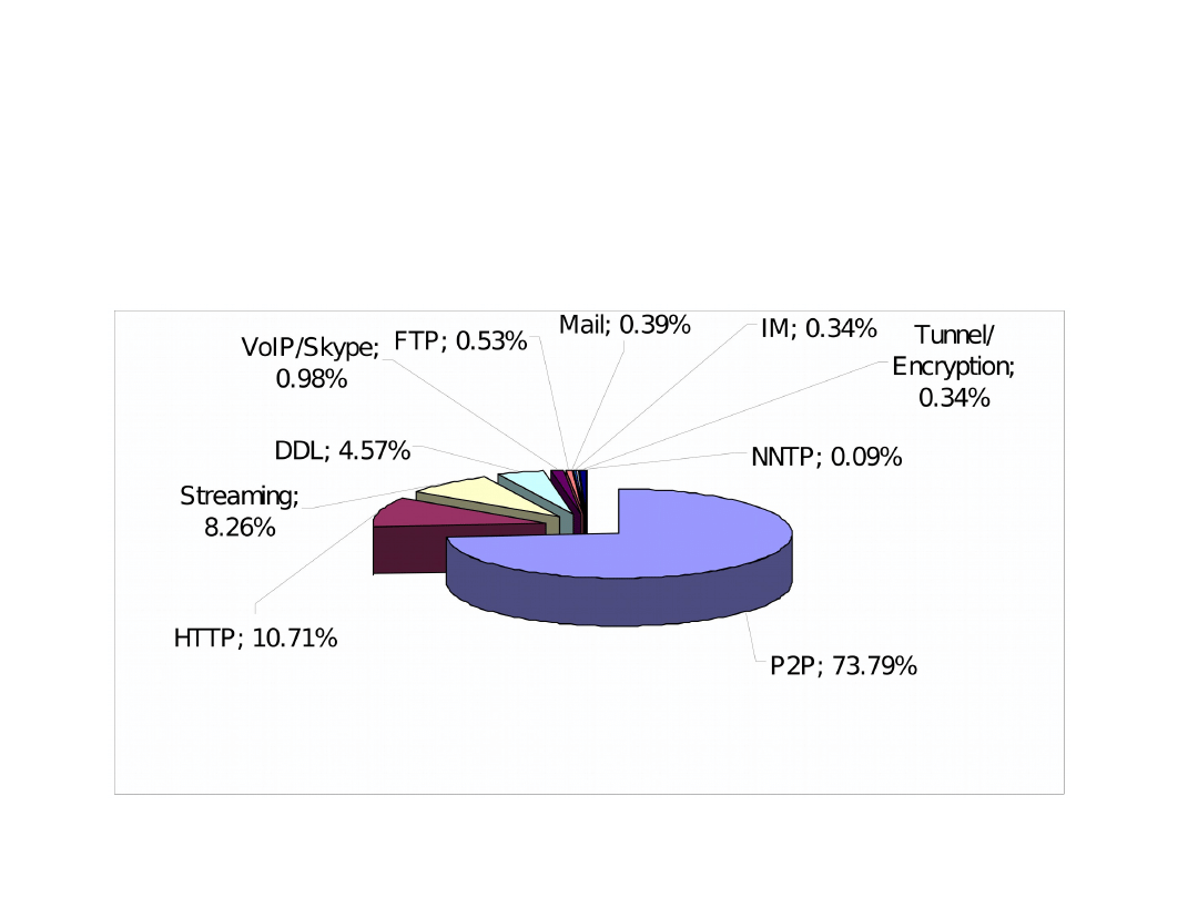
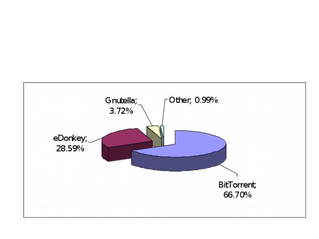
• More than 50% of network traffic in the Internet

is produced by Peer-to-Peer (P2P) systems

• Currently used P2P systems are not aware of

underlying physical network

• Optimizing of flows in P2P systems can reduce

costs and enable better understanding of these

systems

Introduction (2)

Introduction (3)

P2P systems (1)

• Unstructured

 Centralized (Napster)
 Decentralized (Gnutella 0.4)
 Hybrid (Gnutella 0.6)

• Structured (DHT – Distributed Hash Table)

P2P systems (2)

Taking into account the time scale of the P2P

system we can say about:

• Asynchronous – the time scale is without any

constraints. Research: real systems, stochastic
systems

• Synchronous – the time scale is divided into

slots (iterations). Research: offline models,
simulators

P2P systems (3)

Taking into account the dynamics of the P2P system

we can say about:

• Dynamic P2P systems – peers frequently join and

leave the system, e.g., file sharing systems

• Static P2P systems - peers interested in

participating in the system do not leave the
session so frequently, e.g., P2P multicasting
system applied for dissemination of critical
information, streaming system using STBs (set-
top boxes)

P2P systems (4)

The content to be distributed through P2P

multicasting can be divided into two categories:

• Elastic content (e.g. data files - BitTorrent)
• Streaming content with specific bit rate

requirements (e.g. media streaming, P2P
multicasting)

Lecture Outline

• Introduction

• Synchronous P2P Modeling

• P2P Multicast Modeling
• Synchronous P2P Cost Problem
• Other Formulations of Synchronous P2P
• P2P Multicast Network Design Problem
• Concluding Remarks

Assumptions (1)

• The P2P system works on the top of an overlay

network

• The underlying network is overprovisoned, i.e.

the only potential bottlenecks are access links

• Files to be transferred in the network are divided

into blocks of the same size

• There is an indexing service that provides

information on location and availability of blocks

in network nodes

• This service can be implemented as centralized

(e.g. tracker of BitTorrent) or decentralized (e.g.

DHT)

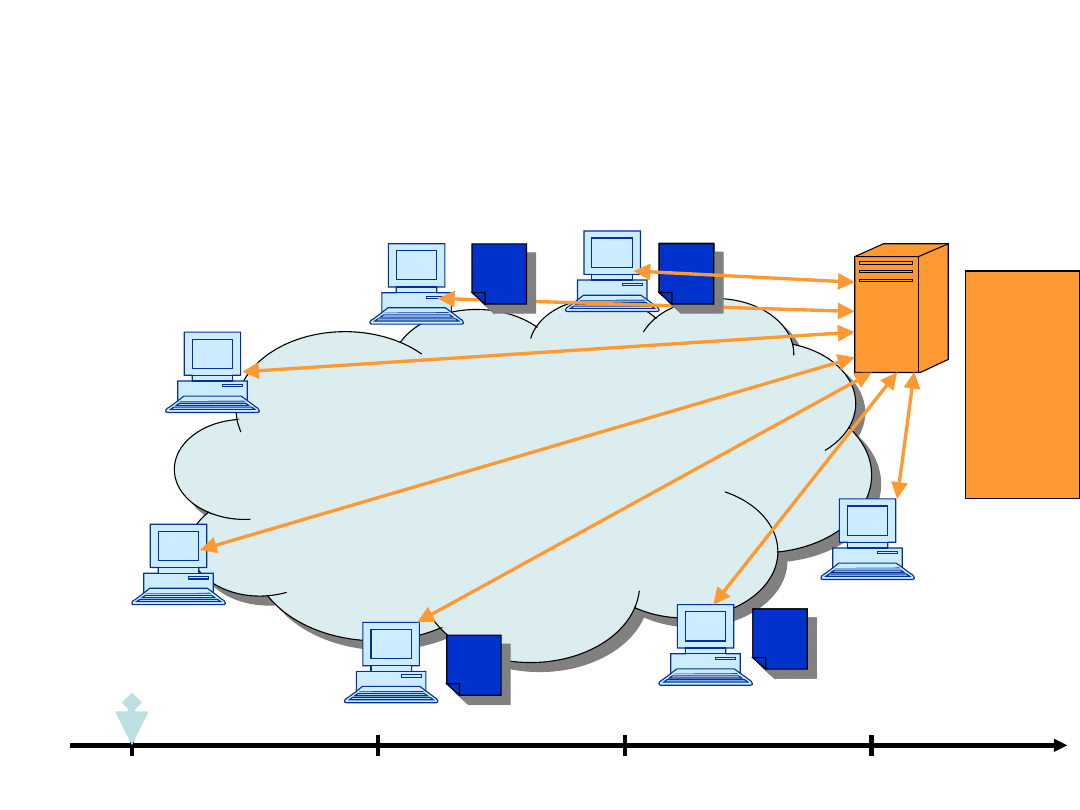
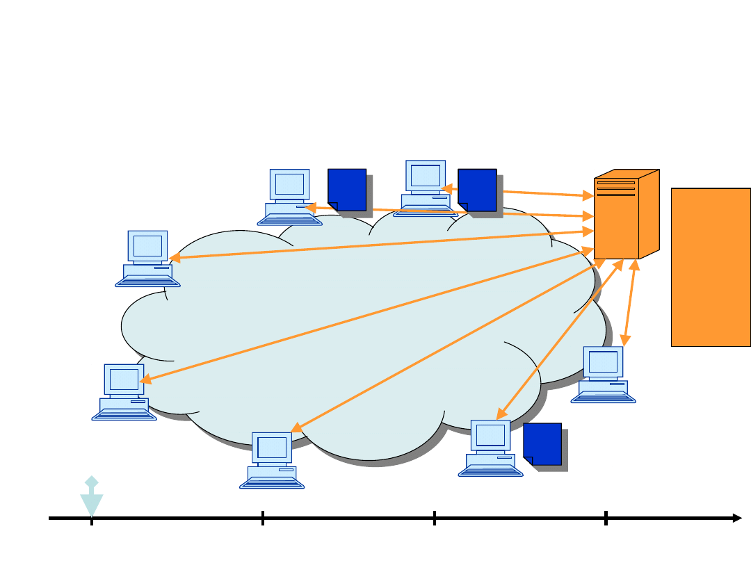
Assumptions (2)

• The system runs in iterations, i.e. the processing

is divided into timeslots

• Blocks are transferred during time slots, the

transfer of one block between two peers takes

just one time slot

• At the end of each time slot (iteration) the index

service updates the information on location and

availability of blocks

• For instance, if block b was transferred to vertex

(peer) v in time slot t, then all other peers can try

to get this block from v in time slot (t+1)

Example, upload=1

1

t=0

t=1

t=2

t=3

2

3

4

5

6

7

1

6

2,5

3,4,7

Example, upload=2

1

t=0

t=1

t=2

t=3

2

3

4

5

6

7

1

2,6

3,4,5,7

Model (1)

indices
b = 1,2,…,B

blocks (pieces)

w,v,s = 1,2,…,V vertices (peers, network nodes)
t = 1,2,…,T

time slots (iterations)

constants
g

bv

= 1, if block b is located in node v before the

P2P

transfer starts (v is the seed); 0,

otherwise

Model (2)

constants
d

v

maximum download rate of node v

u

v

maximum upload rate of node v

M

large number

variables
y

bwvt

= 1, if block b is transferred to node v from

node w in

iteration t; 0, otherwise (binary)

Model (3)

constraints

g

bv

 + 

w



t

 y

bwvt

 = 1,   

b = 1,2,…,B   v = 1,2,…,V



b



v

 y

bwvt

  a

wt

u

w

,  

w = 1,2,…,V   t = 1,2,

…,T



b



w

 y

bwvt

  a

vt

d

v

,  

v = 1,2,…,V   t = 1,2,

…,T



v

 y

bwvt

  M(g

bw

 + 

i < t



s

 y

bswi

),   b = 1,2,…,B

w = 1,2,…,V

t = 1,2,…,T.

Lecture Outline

• Introduction
• Synchronous P2P Modeling

• P2P Multicast Modeling

• Synchronous P2P Cost Problem
• Other Formulations of Synchronous P2P
• P2P Multicast Network Design Problem
• Concluding Remarks

Assumptions

• Overlay P2P multicasting (application-layer

multicast) uses a multicast delivery tree

constructed among peers (end hosts)

• Different to traditional IP multicast, the

uploading (non-leaf) nodes in the tree are

normal end hosts

• Peers are connected to the overlay network,

which is considered as an overprovisioned cloud

- capacity constraints are set only on access links

• The graph is fully connected, i.e. each peer can

connect to any other peer

• Various multicast formulations can be used

(e.g., flow, level)

Example

1

2

3

4

5

6

7

Model (1)

indices
v,w = 1,2,…,V

network nodes

k = 1,2,…,D

receiving nodes (peers)

constants
d

v

download capacity of node v (kbps)

u

v

upload capacity of node v (kbps)

r

v

= 1, if link v is the root of streaming; 0,

otherwise

h

streaming rate (kbps)

Model (2)

variables
x

wvk

  = 1, if in multicast tree the streaming path

from the root to node k includes an overlay link

from node w

to node v (no other peer nodes in

between); 0,

otherwise (binary)

x

wv

  = 1, if the link from node w to node v (no

other peer

nodes in between) is in multicast

tree; 0, otherwise

(binary)

Model (3)

constraints


w

 x

wvk

– 

w

 x

vwk

 = 1,   v = k   v = 1,2,…,V  k =  1,2,

…,K 



w

 x

wvk

– 

w

 x

vwk

 =  –1, r

v

 = 1   v = 1,2,…,V  k =  1,2,

…,K



w

 x

wvk

– 

w

 x

vwk

 = 0, v  k   r

v

  1     v = 1,2,…,V  k = 

1,2,…,K

x

wvk

  x

wv

,

    v = 1,2,…,V   w = 1,2,…,V   k = 1,2,…,K



w

 x

wv

h  d

v

,

   v = 1,2,…,V



v

 x

wv

h  u

w

,

   w = 1,2,…,V



v



t

 x

vvt

 = 0.

Lecture Outline

• Introduction
• Synchronous P2P Modeling
• P2P Multicast Modeling

• Synchronous P2P Cost Problem

• Other Formulations of Synchronous P2P
• P2P Multicast Network Design Problem
• Concluding Remarks

Synchronous P2P Cost Problem

(1)

• The synchronous model of P2P system is used

(time slots)

• Currently used P2P systems generally choose

logical neighbors at random, therefore they

ignore the underlying Internet topology and ISP

link costs

• Since, P2P system has no impact on the

underlying layer (e.g., IP), the transfers are not

optimized in terms of download paths length

• Consequently, there are many cross-continental

and cross-ISP downloads that can congest

backbone networks and generate additional

operating costs for ISPs

Synchronous P2P Cost Problem

(2)

• Localization of peers and information for costs

can be obtained using:

– IP location databases
– Match IP addresses with the same prefix
– Traceroute records

Synchronous P2P Cost Problem

(3)

• We use a broad-spectrum constant



wv

that is

defined as cost of one block transfer between
peers w and v

• It can be interpreted arbitrarily according to our

needs:

– number of hops between w and v
– number of ISPs between w and v
– RTT between w and v
– distance in kilometers between w and v
– cost of cross-ISP transfers

Synchronous P2P Cost Problem

(4)

• An important characteristic of P2P systems is

dynamics – peers can frequently join or leave
the network

• To model this phenomenon we use constants a

vt

,

which equals to 1, if peer v in time slot t is
connected to the network (is available) and 0,
otherwise

• Consequently, although the model is

deterministic, the stochastic nature of P2P system
can be incorporated into the considerations

Synchronous P2P Cost Problem

(5)

Given: overlay network topology, peers, seed

location, access link capacity, link availability, link
cost, number of blocks, number of time slots

Minimize: cost

Over:P2P synchronous routing

Synchronous P2P Cost Problem

(6)

indices
b = 1,2,…,B

blocks (pieces)

w,v = 1,2,…,V

vertices (peers, network nodes)

t = 1,2,…,T

time slots (iterations)

constants
g

bv

= 1, if block b is located in node v before the

P2P

transfer starts (v is the seed); 0,

otherwise



wv

cost of block transfer from node w to node v

a

vt

= 1, if node v is available in time slot t;

0, otherwise

Synchronous P2P Cost Problem

(7)

constants
d

v

maximum download rate of node v

u

v

maximum upload rate of node v

M

large number

variables
y

bwvt

= 1, if block b is transferred to node v from

node w in

iteration t; 0, otherwise (binary)

Synchronous P2P Cost Problem

(8)

objective
minimize   F = 

b



v



w



t

 y

bwvt

 



wv

constraints
g

bv

 + 

w



t

 y

bwvt

 = 1,   

b = 1,2,…,B  v = 1,2,…,V



b



v

 y

bwvt

  a

wt

u

w

,

   

w = 1,2,…,V  t = 1,2,…,T



b



w

 y

bwvt

  a

vt

d

v

,

   

v = 1,2,…,V  t = 1,2,…,T



v

 y

bwvt

  M(g

bw

 + 

i < t



s

 y

bswi

),   b = 1,2,…,B w = 1,2,

…,V

t = 1,2,…,T.

Optimization

• The problem is linear, integer (binary) and

NP-complete (equivalent to MBT (Minimum
Broadcast Time) problem)

• To find optimal solutions solvers like CPLEX and

GuRoBi can be used

• Heuristics can be used, e.g., constructive,

random, evolutionary algorithm, etc.

Algorithms (1)

1 for t=1 to T
2 begin
3 while (IsPossibleTranfer(t))
4 begin
5 v=RandomDownloadPeer(t)
6 b=SelectBlock(v,t)
7 w=SelectUploadPeer(b,v,t)
8 TransferBlock(b,w,v,t)
9 end (if)
10 end (for)

Algorithms (2)

Functions SelectBlock and SelectUploadPeer have

different versions according to a particular strategy:

• Random Strategy (RS) – selects the block and

upload peer at random among all feasible blocks

and upload nodes

• Rarest First Strategy (RFS) function SelectBlock

returns the rarest feasible block in the network, the

upload peer is chosen at random

• Cost Selection Strategy (CSS) – takes into

account transfer costs, the block to be transferred

is selected at random, but the closest, feasible peer

is chosen for upload

• Weighty Piece Selection Strategy (WPSS)

Results (1)

• To solve the model in optimal way we apply

CPLEX 11.0

• Since the goal is to compare results of BitTorrent-

like systems simulations against optimal results,
we had to limit size of the problem instances
in order to obtain optimal results approximately in
one hour

• After several experiments we decide to test

networks consisting of 10 vertices (peers), 3
blocks to be transferred and 4 time slots

Results (2)

• Peers are located in large cities worldwide
• The cost of one block transfer between two peers

located in two cities just as the distance in
kilometers between these two cites

• Three networks were tested:

– E5A5 – 5 peers in Europe and 5 peers in North

America

– E7A3 – 7 peers in Europe and 3 peers in North

America

– E10 – 10 peers in Europe

Results (3)

• Three scenarios of access link capacity:

– asymmetric (upload=2 blocks, download=4

blocks)

– symmetric (upload=2 blocks, download=2

blocks)

– random (upload and download is selected

randomly between 2 blocks and 4 blocks)

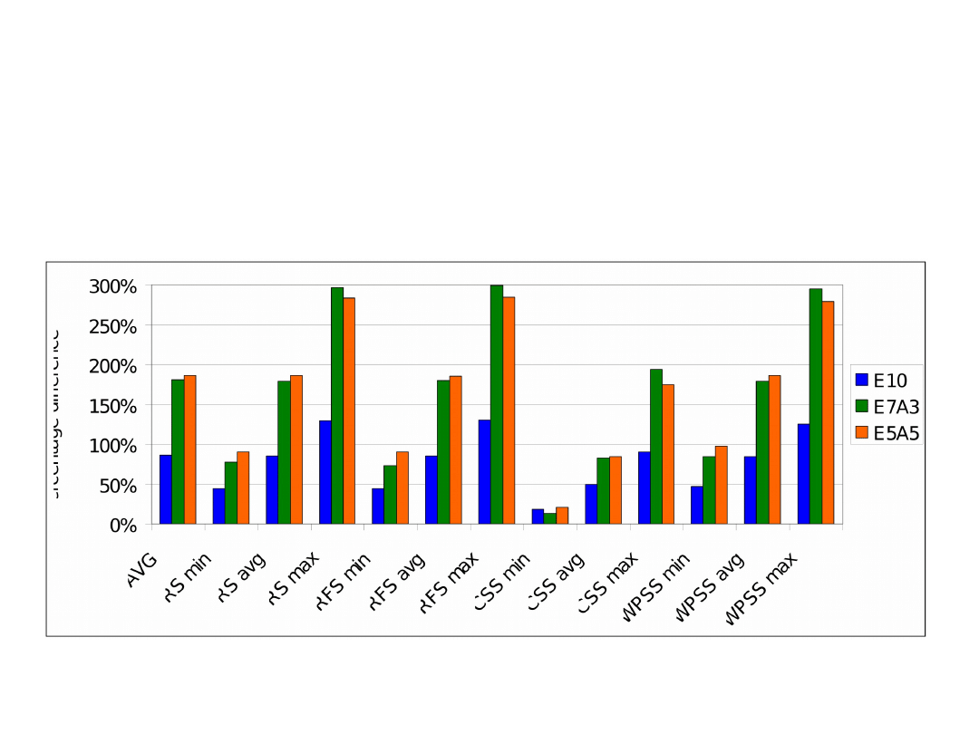
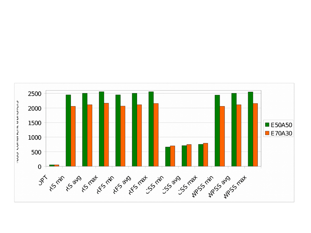
Average distance to optimal results for various

networks

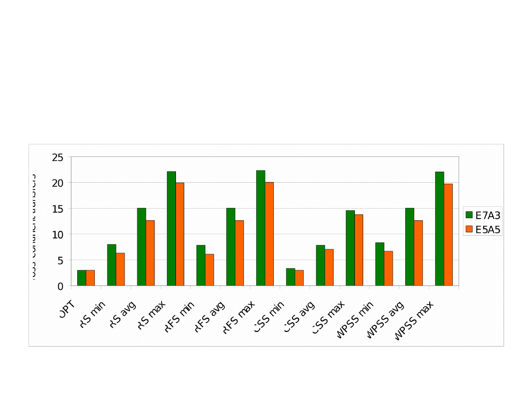
Average number of cross-continent transfers

for various networks

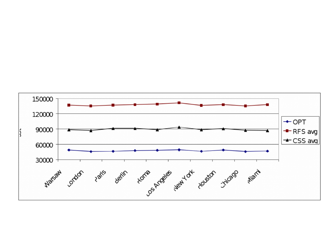
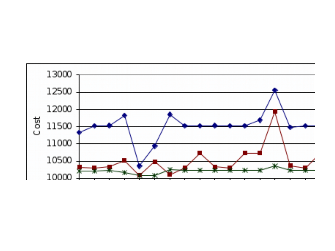
Heuristics against optimal results obtained for

network E5A5 as a function of seed location

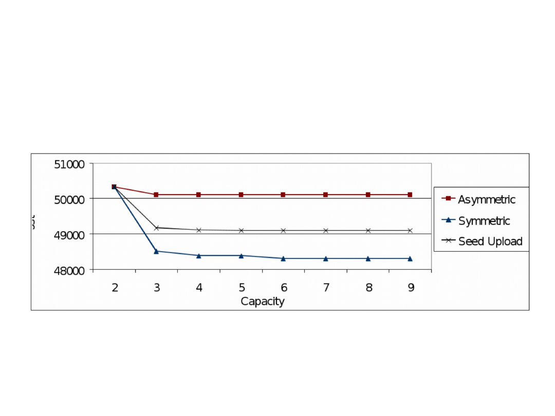
Optimal results obtained for network E5A5 as a

function of upload capacity

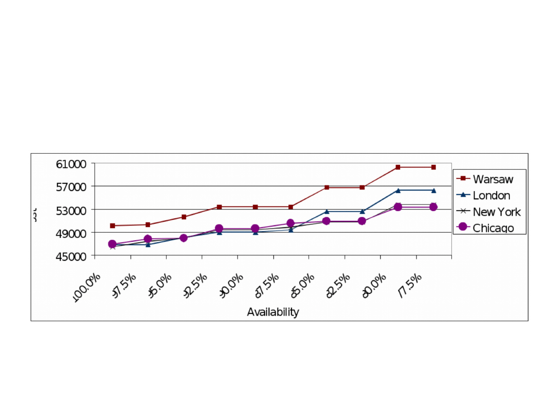
Optimal results obtained for network E5A5 as a

function of peer availability and seed location

Average number of cross-continent transfers for

various networks (100 nodes, 50 blocks, 40 time

slots)

Lecture Outline

• Introduction
• Synchronous P2P Modeling
• P2P Multicast Modeling
• Synchronous P2P Cost Problem

• Other Formulations of Synchronous P2P

• P2P Multicast Network Design Problem
• Concluding Remarks

Download Time Objective

• In the model the download time is represented

by T – a constant denoting the number of time

slots

• If T a is used as the objective function, the

problem becomes a Non-linear Integer Problem

• The following procedure can be employed to find

the minimal value of T

– Set T to some value
– Solve the IP problem consisting of P2P system

constraints (selected among those presented above)

– If the problem has a feasible solution, then decrease T

by 1; otherwise increase T by 1

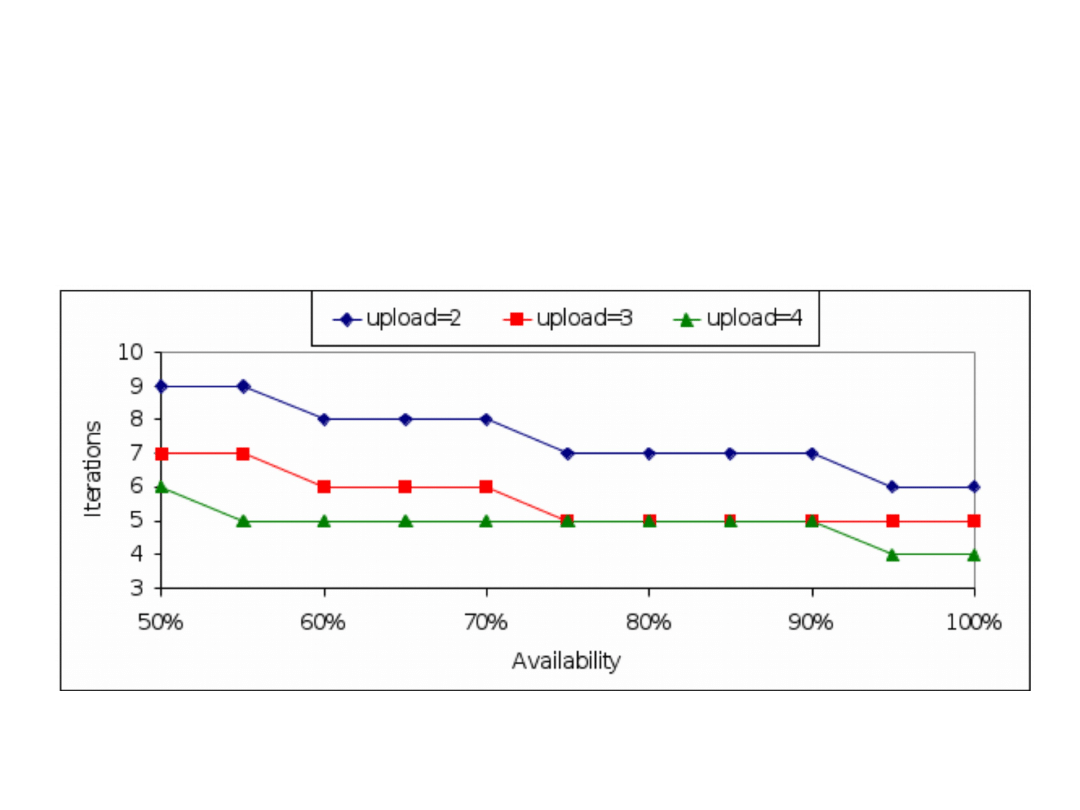
The download time as a function of availability for

various values of upload capacity

Throughput

• Throughput of the P2P system, which is defined

as the number of blocks (which can be
interpreted as the size of a file) that can be
transferred to every node within given time slots

• In the model this is denoted by B – a constant

denoting the number of blocks

• The procedure to solve the IP problem with the

throughput as the objective can be the same as
in the case of the download time

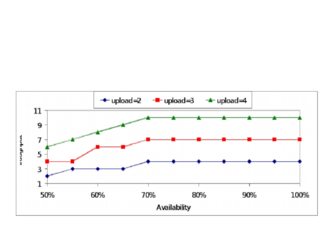
The system throughput as a function of availability

for various values of upload capacity

Fairness Constraint

• The P2P system should be fair in terms of the

number of blocks served by the individual nodes

• Fairness can be viewed as a kind of an incentive

for nodes to participate, especially in situations
where ISPs charge based on uplink usage or
uplink bandwidth is scarce

• To enforce fairness in the P2P system we add

constraint



b



w



t

 y

bvwt

  



 

b



w



t

 y

bwvt

   v = 1,2,…,V

• Constant



denotes the fairness of the system

Neighbors Constraint

• In the BitTorrent protocol a new peer joining the

system asks the tracker for a list of peers to
connect to and cooperate with (exchange blocks)

• Such peers are called neighbors
• To model this we introduce a constant e

wv

which

equals 1 if peers w and v are neighbors, 0
otherwise

• Next a following condition can be formulated



b



t

 y

bwvt

  Me

wv

   w = 1,2,…,V  v = 1,2,…,V

Lecture Outline

• Introduction
• Synchronous P2P Modeling
• P2P Multicast Modeling
• Synchronous P2P Cost Problem
• Other Formulations of Synchronous P2P

• P2P Multicast Network Design Problem

• Concluding Remarks

Network Design Problem (1)

• CFA (Capacity and Flow Allocation) problem
• Multiple trees using for streaming
• Level formulation of multicast flows
• Candidate access links
• Each peer has background traffic (download

and upload)

Network Design Problem (2)

Given: network topology, root location, number of

trees, streaming rates, background traffic

Minimize: network cost

Over:P2P multicast routing, link allocation

Network Design Problem (3)

indices
w,v = 1,2,…,V

overlay network nodes (peers)

k = 1,2,…,K

v

access link types for node v

t = 1,2,…,T

trees

l = 1,2,…,L levels of the multicast tree
constants
a

v

download background transfer of node v

b

v

upload background transfer of node v

Network Design Problem (4)

constants



vk

cost of link type k for node v

d

vk

download capacity of link type k for node v

(kbps)

u

vk

upload capacity of link type k for node v

(kbps)

r

v

= 1, if node v is the root of the tree; 0,

otherwise

h

t

the streaming rate of tree t (kbps)

M

large number

Network Design Problem (5)

variables
x

wvtl

= 1, if there is a link from node w to node v is

in multicast tree t and w is located on level l of
tree

t; 0, otherwise (binary)

y

vk

= 1, if node v is connected to the overlay

network by

a link of type k; 0, otherwise

(binary)

objective
minimize   F = 

v



k

 y

vk



vk

Network Design Problem (6)

constraints


w



l

 x

wvtl

 = (1 – r

v

), 

v = 1,2,…,V   t = 1,2,…,T



v

 x

wvt1

  Mr

w

,

   

w = 1,2,…,V   t = 1,2,…,T

x

wvt(l+1)

  

s

 x

swtl

,

   

v = 1,2,…,V   w = 1,2,

…,V

t = 1,2,

…,T  l = 1,2,…,L – 1



k

 y

vk

 = 1,   

v = 1,2,…,V

a

v

 + 

t

 h

t

  

k

 y

vk

d

vk

,

    v = 1,2,…,V

b

w

 + 

vw



t



l

 x

wvtl

h

t

  

k

 y

wk

u

wk

,

   w = 1,2,…,V.

Optimization

• The problem is linear, integer (binary) and

NP-complete (equivalent to unicast network
design problem)

• To find optimal solutions solvers like CPLEX and

GuRoB can be used

• Heuristics can be used, e.g., construction

algorithms, Lagrangean Relaxation, evolutionary
algorithm, etc.

Algorithm Create Tree (1)

• Create Tree is a constructive algorithm using the

following functions

• We assume that for each node v = 1,2,…,V the

access link types are sorted according to

increasing values of upload capacity and cost.

• Tree t is feasible on level l if there is at least one

possible transfer from node v (located on level l

of tree t) to node w

• Let ftree(l) return an index of a feasible tree on

level l. If there is more than one feasible tree, we

select the tree with the lowest number of nodes

connected to the tree

Algorithm Create Tree (2)

• Node v is a feasible parent node on level l of

tree t if there is at least one possible transfer in

tree t on level l between v and any other node

• Let fpnode(t, l) return an index of a feasible

parent node located on level l of tree t. If there is

more than one feasible parent node, the

algorithm chooses the node with the largest value

of residual upload capacity

• Let fcnode(v, t, l) return an index of a feasible

child node of node v located on level l of tree t . If

there is more than one feasible child node, again

the residual upload capacity is the additional

criterion

Algorithm Create Tree (3)

• Let istrasnfer(l) return 1 if there is at least one

possible transfer on level l of any tree, 0 otherwise

• If each node v = 1,2,…,V is connected to each tree

t = 1,2,…,T, i.e. all necessary transfers are

completed, function istree() returns 1; otherwise

it returns 0

• Function isupdate() returns 1 if incrementing of

the access link upload capacity is possible for at

least one node; 0 otherwise.

• We assume that first(A) returns the first element

of table A

• Let h = t h

t

  denote the overall streaming tree

rate of all trees

Algorithm Create Tree (4)

• Let function updatenode() return an index of a

node v, for which the upload capacity can be
augmented. If there is more than one such a
node, an additional criterion is applied. In the
algorithm we use several combinations of two
values: node level and relative cost of upload
capacity increase given by the formula
(u

v(k+1)

 – u

vk

) / (



v(k+1)

 – 



vk

)

Algorithm Create Tree (5)

Step 0. Set x

wvtl

 = 0 for each w = 1,2,…,V, v = 1,2,

…,V, t = 1,2,…,T, l = 1,2,…,L, v  w.

Set y

vk

as the minimal values that guarantee

sufficient download capacity for each node v
expect the root node (i.e. d

vk

  a

v

 + h) and the

sufficient upload capacity for the root node r (i.e.
u

rj

  b

r

 + h).

Algorithm Create Tree (6)

Step 1. Set l = 1. Create table A containing all trees

sorted in decreasing order of streaming rate q

t

.

Create table B containing all nodes except the root
node sorted in decreasing order of residual upload
capacity of each node.

a)  If A =  go to Step 2. Otherwise, go to Step 1b.
b) Calculate t = first(A), v = first(B) and x

rvtl

 = 1.

Next, set A = A – {t} and B = B – {v}. Go to Step
1a.

Algorithm Create Tree (7)

Step 2. If l > L go to Step 3
a)  If istrasnfer(l) = 0 set l = l + 1 and go to Step 2.

Otherwise go to Step 2b.

b)  Set t = ftree(l), w = fpnode(t, l), v = fcnode(v, t, l)

and x

wvtl

 = 1. Go to Step 2a

Step 3. If istree() = 1 stop the algorithm, a feasible

solution exists. Otherwise, go to Step 4.

Step 4. If isupdate() = 0, stop the algorithm, there is

not feasible solution. Otherwise, go to Step 5.

Step 5. Set v = updatenode(). Find k, for which

y

vk

 = 1. Set y

vk

 = 0, k = k + 1, y

vk

 = 1, l = 1 and go

to Step 2

Results (1)

• We use DSL price lists of four ISPs: two of them

operate in Poland (TP and Dialog) and two other

operate in Germany (DT and Arcor)

• Each node is randomly assigned to one of ISPs

and selects any option included in the price list

• The values of download background transfer

are selected at random between 512 kbps and

1024 kbps

• Analogously the values of upload background

transfer were selected at random between 64

kbps and 128 kbps

Results (2)

• To obtain optimal results we use CPLEX 11.0

solver

• Due to complexity of the problem only for small

networks (20 nodes) the CPLEX can yield
optimal results in reasonable time of
approximately one hour

• The number of multicast trees was in the range

1-4

• The number of levels was in the range 2-8
• We compared the Create Tree algorithm also

against Lagrangean Relaxation algorithm

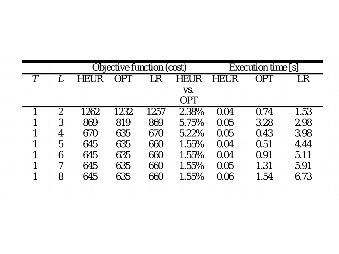
Heuristic algorithm versus optimal results and

Lagrangean relaxation results

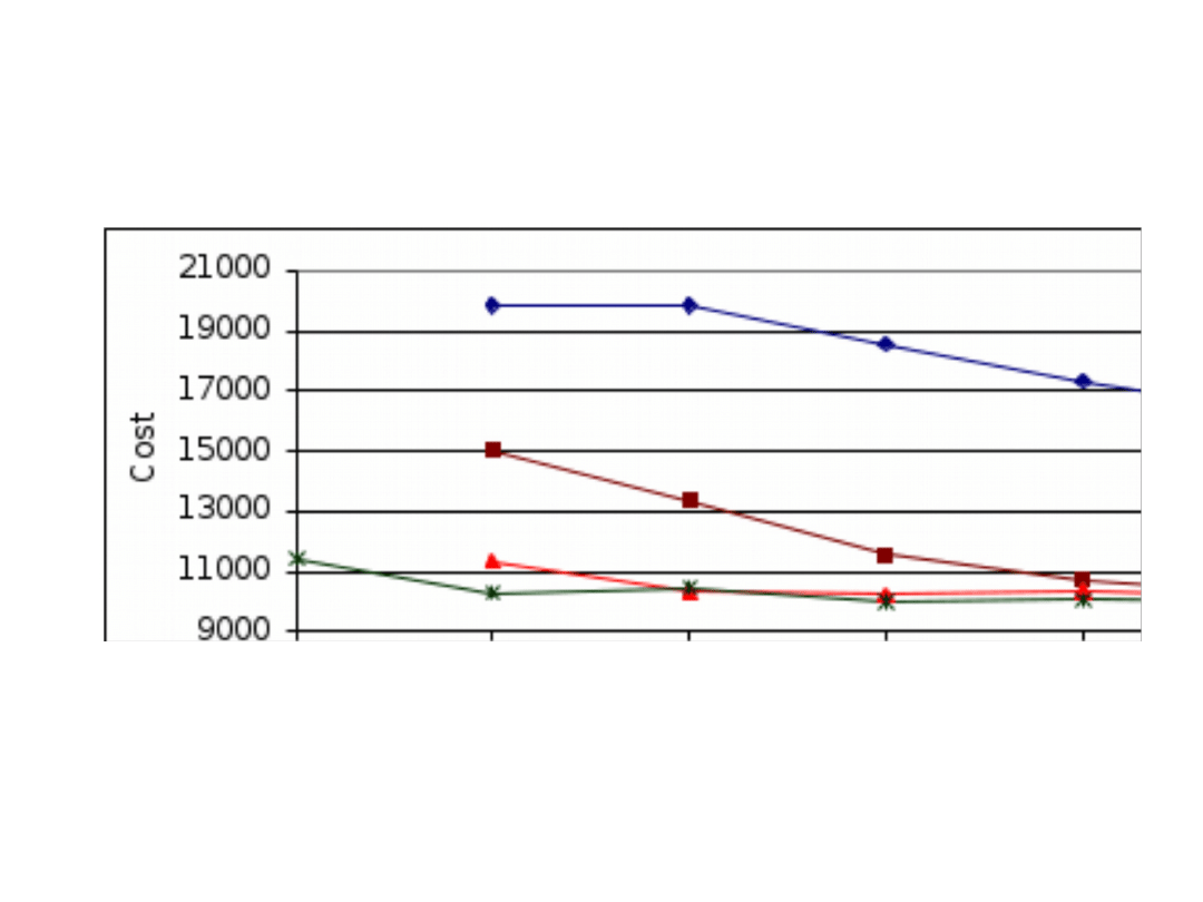
The network cost as a function of tree levels for

various number of multicast trees

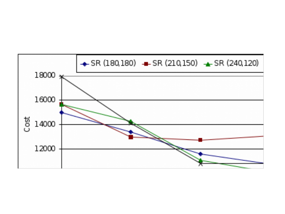
The network cost as a function of tree levels for 2

trees and various scenarios of streaming rate (SR)

split

The network cost as a function of the root location

for various values of tree levels

Lecture Outline

• Introduction
• Synchronous P2P Modeling
• P2P Multicast Modeling
• Synchronous P2P Cost Problem
• Other Formulations of Synchronous P2P
• P2P Multicast Network Design Problem

• Concluding Remarks

Concluding Remarks

• Most of P2P systems work in the overlay mode
• The main problem in modeling of P2P systems is

the dynamics in the time scale

• Synchronous models with the time scale have

been presented

• In static P2P systems formulations based on

multicast flows can be used with additional

constraints following from the overlay network

• Optimization of P2P models, especially with the

time scale is very complicated due to the

problem size

Further Reading

• Buford J., Yu H. and Lua E., P2P Networking and Applications,

Morgan Kaufmann, 2009

• Steinmetz R. and Wehrle K. (eds.), Peer-to-Peer Systems and

Applications, Lecture Notes in Computer Science, Vol. 3485,

Springer Verlag, 2005

• Wu C. and Li B., Optimal Rate Allocation in Overlay Content

Distribution, in Proc. of the 6th Networking Conf., 2007, pp. 678-690

• Zhu Y. and Li B., Overlay Networks with Linear Capacity Constraints,

IEEE Transactions on Parallel and Distributed Systems”, vol. 19,  no.

2, 2008, pp. 159-173

• Walkowiak K. , Offline Approach to Modeling and Optimization of

Flows in Peer-to-Peer Systems, in Proc. of the New Technologies,

Mobility and Security Conference, NTMS '08, 2008

• Walkowiak K. , Network Design Problem for P2P Multicasting, in

Proc. of the International Network Optimization Conf. INOC, 2009

• Walkowiak K., Dimensioning of Overlay Networks for P2P

Multicasting, in Proc. of the 12th IEEE/IFIP Network Operations and

Management Symposium (NOMS 2010), 2010, pp. 805-808