J Comput Virol (2010) 6:31–42
DOI 10.1007/s11416-008-0111-3

O R I G I NA L PA P E R

Analysis of a scanning model of worm propagation

Ezzat Kirmani

· Cynthia S. Hood

Received: 29 May 2008 / Accepted: 7 December 2008 / Published online: 24 December 2008
© Springer-Verlag France 2008

Abstract The traditional approach to modeling of internet
worm propagation is to adopt a mathematical model, usually
inspired by modeling of the spread of infectious diseases,
describing the expected number of hosts infected as a func-
tion of the time since the start of infection. The predictions of
such a model are then used to evaluate, improve, or develop
defense and containment strategies against worms. However,
a proper and complete understanding of worm propagation
goes well beyond the mathematical formula given by the
chosen model for the expected number of hosts infected
at a given time. Thus, questions such as fitting the model,
assessing the extent to which a specific realization of a worm
spread may differ from the model’s predictions, behavior of
the time points at which infections occur, and the estimation
and effects of misspecification of model’s parameters must
also be considered. In this paper, we address such questions
for the well-known random constant spread (RCS) model
of worm propagation. We first generalize the RCS model to
our nonhomogeneous random scanning (NHRS) model. The
NHRS model allows the worm’s contact rate to vary during
worm propagation and it thus captures far more situations of
interest than the RCS model which assumes a scanning rate
constant in time. We consider the problem of fitting these
models to empirical data and give a simulation procedure for
a RCS epidemic. We also show how to obtain a confidence
interval for the unknown contact rate in the RCS model. In
addition, the use of prior information about the contact rate

E. Kirmani (

B

)

Department of Statistics and Computer Networking,
Saint Cloud State University, Saint Cloud, MN 56301, USA
e-mail: [e-mail]

C. S. Hood
Department of Computer Science, Illinois Institute of Technology,
Chicago, IL 60616, USA
e-mail: [e-mail]

is discussed. The results and methodologies of this paper
illuminate the structure and application of NHRS and RCS
models of worm propagation.

1 Introduction

Internet worms such as Code Red, Nimda, Slammer, and
Blaster have dramatically exposed the vulnerability of the
Internet to malicious programs that self-propagate by exploit-
ing software errors and other security faults. The recent trend
in malware towards bots and botnets has not, by any means,
eliminated the challenge of worms. In fact, as noted in Lee
et al. [

6

], botnets can provide a platform for simultaneous

launching of worms from distributed networks of bots. Such
an instantaneous attack necessarily shortens the window of
time in which the network administrators must implement
the necessary countermeasures. Apparently, the art and sci-
ence of defense and containment methodologies against such
worms is lagging behind. The development of countermea-
sures depends, among other things, on the worm’s function
structure, its execution mechanism, scanning strategies, and
propagation modeling (see [

11

] for a brief survey). The tra-

ditional approach to modeling of internet worm propagation
is to choose a mathematical model describing relationships
of interest, such as the expected number of hosts infected as
a function of the time since the start of infection. The pre-
dictions of such a model are then used in evaluating defense
and containment strategies against worms. Thus, mathemat-
ical models of worm propagation play an important role
and it is necessary to understand their limitations, structure,
ramifications, and how they are applied to specific situa-
tions. Some important questions in this regard are estimation
of the unknown parameters of a worm propagation model,
simulation of various realizations to assess deviations from

123

32

E. Kirmani, C. S. Hood

predicted behavior, and sensitivity of the model to misspeci-
fications of parametric values. The objective of this paper
is to study selected such aspects of the well-known ran-
dom constant spread (RCS) model of worm propagation and
its generalization to a model allowing for nonhomogeneous
contact rates.

In order to evaluate, improve, and develop effective

defense and containment strategies against such worms it
is necessary to understand how various worms propagate.

Although models for the spread of computer virus were

already considered in [

4

,

5

], it was the Code Red worm of

July, 2001 which led to wide interest in modeling of internet
worm propagation [

9

]. Staniford et al. [

13

] used empirical

data derived from the outbreak of the Code Red worm to
develop their RCS model. It describes the cumulative num-
ber of hosts infected, as a function of the time since the start of
the worm epidemic, in the absence of any measures to counter
the epidemic. It is useful in predicting the propagation pat-
tern of new worms. This model has become a benchmark
and a source of extensions, generalizations, and refinements.
A key assumption in this model is that the rate at which an
infected host chooses new victims is constant in time. This,
of course, is a simplification which ignores that most hosts
have different bandwidths available for scanning and differ-
ent scanning computing power. Moreover, large scale worm
propagation causes network congestion resulting in actually
slowing down the worm’s contact rate after a certain thresh-
old. The constant scanning rate in a RCS model is thus merely
an average which has obvious limitations in describing the
evolution of infection in time. We, therefore, develop a gen-
eralization of the RCS model in which the worm’s scanning
rate is not constant but varies with time. This improvement,
which we call the nonhomogeneous random scanning model
(NHRS), is presented in Sect.

2

.

In Sect.

2

, we also show how to fit our NHRS model using

minimal empirical data. We also give a procedure based on
linear regression, to estimate the contact rate of a RCS worm
and assess the goodness-of-fit of the RCS model. The gen-
eral approach to worm propagation models in the literature
is to consider the number of infected hosts as a deterministic
function of the time since the start of the epidemic. While
this approach does give the expected number of infected
hosts, it fails to explain the probabilistic structure underlying
worm propagation. The importance of fully understanding
the probabilistic regime of worm behavior has not been prop-
erly appreciated in the literature although Nicol [

10

] made a

strong case for studying the impact of stochastic variance on
worm propagation and detection. As noted in Nicol [

10

], the

regime of worm behavior affects simulation-based studies of
worm detection/defense mechanisms. The complete probabi-
listic description of worm propagation requires specification
of the probability distribution of the sequence of successive
infection times. Indeed, this is our approach in Sect.

3

. It

enables us to fully explain the probabilistic regime of worm
propagation for NHRS and RCS models. Our results in Sect.

3

provide the basis for a sound probabilistic procedure for sim-
ulating a RCS epidemic. This procedure, included in Sect.

3

itself, enables us to simulate worm propagation in order to see
the extent to which a specific realization may differ from the
prediction of the RCS model. Such simulations are impor-
tant for quantitative assessment of effectiveness of detection
mechanisms and countermeasures.

The constant contact rate assumed in the RCS model is

generally unknown. In addition to the linear regression based
method of Sect.

3

, we give a confidence interval for the

contact rate in Sect.

4

. The data required for this confidence

interval is merely the number of hosts infected during an
observation period. Since the exact value of the contact rate is
unknown, it is important to be able to assess the sensitivity of
the predictions made by the RCS model. We address this issue
in Sect.

4

by deriving the expected number of hosts infected

during any specified time by adopting a Bayesian approach.
We conclude with a brief description of future work on an
extension of the NHRS model to include possible recovery,
patching and immunization of systems.

2 RCS model and its nonhomogeneous improvement

NHRS model

Creating workable models of worm propagation is necessary
for several reasons. They allow us to learn form previous
worm incidents and to possibly predict the behavior of future
worms. They help to develop and test containment, disin-
fection, and patching strategies without actually developing
and releasing computer worms. Moreover, worm propaga-
tion models appear to be the sole means for predicting the
extent of failure and damage a worm may cause to the Inter-
net. This prediction is particularly important for the early
phase of worm propagation. In the early phase, the necessary
defenses may not be in place which it may be crucial to pre-
vent the worm from spreading into critical parts of networks.

A crucial factor in the propagation of a worm is its spread

algorithm. The most popular spread algorithm is random
scanning in which the worm picks an IP address at random,
attempts to establish contact and infect it. The Code Red
worm employs random scanning. Staniford et al. [

13

] devel-

oped their RCS model to describe the propagation of CRv2,
the second version of the Code Red worm, which attacked
the Internet on July 19, 2001.

2.1 Extending the RCS model to allow time-dependent

contact rate

The RCS model assumes that: (a) the total number of vulnera-
ble hosts which can be potentially compromised is a constant

123

Analysis of a scanning model of worm propagation

33

N , (b) the Internet topology can be considered as an unidi-

rected complete graph, (c) the number of vulnerable hosts
that an infected host can compromise per unit of time is a
constant

β, (d) an infected host picks other hosts to attack

completely at random, and (e) a host cannot be compromised
multiple times. The assumption (a) implies that countermea-
sures such as patching, disconnecting servers or restricting
access are ignored. While unrealistic in general, this may
well be reasonable in the early phase of the propagation of
a new worm for which the necessary defenses may not be in
place. Assumption (b), though not really true, is not a seri-
ous limitation and lack of complete connectivity does not
fundamentally alter the conclusions of the RCS model. The
assumption (c) ignores differences in network connection,
bandwidth, and processor speeds.

The RCS model consists of the differential equation

d

dt

a

(t) = βa(t){1 − a(t)}

(1)

where a

(t) denotes the proportion of vulnerable hosts

infected during the time period

[0, t] with t = 0 as the instant

of infection of the first host(s) infected and

β is the constant

contact rate. If a

(0) = I

0

/N, where I

0

≥ 1, the (

1

) has the

solution

a

(t) =

1

1

+ ψ exp(−βt)

(2)

where

ψ = (N − I

0

)/I

0

.

Staniford et al. [

13

] fitted the RCS model to the total num-

ber of inbound scans seen during

[0, t], 0 < t ≤ 16, t in

hours, on port 80 at the Chemical Abstracts Service during
the initial outbreak of CRv2 on July 19, 2001. The contact
rate

β depends on the worm’s probe rate and its target acqui-

sition function. The solution of (

1

) given by (

2

) requires the

assumption that

β is constant in time. However, large scale

worm propagation causes network congestion affecting the
availability of bandwidth [

2

,

3

]. Such bandwidth limitations

or human reaction actually slows down the worm’s scanning
process. To model this phenomenon, a constant value of

β is

clearly inappropriate; a more realistic assumption, for exam-
ple, might be to take

β as a decreasing function of the number

of hosts infected by time t. In any case, the assumption that
β is constant in time merely assigns an average value to β
which cannot convey the extent and nature of variability in
time.

We, therefore, propose a generalization of the RCS model

by allowing

β to depend on time t. This generalization, given

in Proposition

1

below, will be called the NHRS model. We

will take the number of hosts infected during

[0, t] as a

random variable X

(t) rather than the deterministic function

N a

(t). Although the deterministic function Na(t) can itself

be interpreted as the expected value of X

(t), our approach

has two advantages: (1) it makes the underlying probabilistic

assumptions fully transparent, and (2) enables the deriva-
tion of some useful probability distributions in Sects.

3

and

4

. In keeping with the terminology now commonly used in

the worm propagation literature, we will refer to hosts vul-
nerable to be infected by a worm as susceptible hosts. The
following proposition describes our NHRS model.

Proposition 1 Given a set of N hosts, let I

(t) = E{X(t)}

where X

(t) is the number of hosts infected during the time

period

[0, t], t ≥ 0. Suppose that (i) a host once infected

becomes infectious (i.e., capable of causing infection) and
remains so, (ii) a susceptible host becomes infected if and
only if it comes into contact with an infectious host, (iii)

p

(t, t + t) is the probability that a given susceptible host

is contacted by a given infectious host during the infinitesi-
mal time period

(t, t + t], (iv) this probability is the same

for each pairing of susceptible hosts with infected hosts, and
(v) all contacts between susceptible and infectious hosts are
independent.

If

p

(t, t + t) = {β(t)/N}t + o(t)

(3)

then

(A)

d

dt

I

(t) = β(t)I (t)

I

−

I

(t)

N

, t > 0,

(4)

which has the solution

(B)

I

(t) =

N

1

+ ψ exp(−

t

0

β(u)du)

, t ≥ 0,

(5)

where

ψ =

N

−I

0

I

0

with I

0

= I (0).

Proof In order to prove (A), we must calculate I

(t + t) −

I

(t). This is the expected increase in the number of infected

hosts during

(t, t +t]. It represents the expected number of

infections (among the N

− X(t) hosts susceptible at time t)

during

(t, t + t] generated by the I (t) hosts who are infec-

tious at time t. Therefore,

I

(t + t) − I (t) = E

⎧

⎨
⎩

N

−X(t)

i

=1

C

i

⎫

⎬
⎭

(6)

where

C

i

=

⎧

⎨
⎩

1

, if the i th susceptible host is contacted by

at least one infectious host during

(t, t + t]

0

, otherwise.

In view of the assumptions made above,

I

(t + t) − I (t) = λE{N − X(t)}

= λ{N − I (t)}

(7)

123

34

E. Kirmani, C. S. Hood

where

λ depends on t and t, and, for each i

λ = E(C

i

) = P(C

i

= 1)

=

N

n

=0

P

(C

i

= 1|X(t) = n)P(X(t) = n).

Now, for all n

≥ 1,

P

(C

i

= 1|X(t) = n) = 1 − P(C

i

= 0|X(t) = n)

= 1 − P(the ith susceptible in not contacted by

any of the n infectious hosts during

(t, t + t])

= 1 −

n

j

=1

P

(the ith susceptible in not contacted by

the j th infectious host during

(t, t + t])

= 1 − {1 − p(t, t + t)}

n

= 1 −

n

k

=0

n
k

(−1)

k

{p(t, t + t)}

k

(8)

Since

p

(t, t + t) = {β(t)/N}t + o(t),

we have

{p(t, t + t)}

k

= o(t)

(9)

for all k

≥ 2. Therefore, the last sum above reduces to

np

(t, t + t) + o(t)

so that, for all n

≥ 1,

P

(C

i

= 1|X(t) = n) = np(t, t + t) + o(t).

(10)

Since it is trivial that

P

(C

i

= 1|X(t) = 0) = 0,

we get

λ =

N

n

=0

{np(t, t + t) + o(t)}P(X(t) = n)

= p(t, t + t)

N

n

=0

n P

(X(t) = n) + o(t)

= p(t, t + t)E{X(t)} + o(t)
= p(t, t + t)I (t) + o(t)

=

β(t)

N

t + o(t)

I

(t) + o(t)

=

β(t)

N

I

(t)t + o(t)

(11)

Therefore,

I

(t + t) − I (t)

t

=

λ{N − I (t)}

t

=

β(t)

N

I

(t){N − I (t)} +

o

(t)

t

(12)

Taking the limit as

t −→ 0 and noting that

lim

t−→0

o

(t)

t

= 0,

(13)

we get

d

dt

I

(t) =

β(t)

N

I

(t){N − I (t)}

= β(t)I (t)

1

−

I

(t)

N

which proves claim (A) of the proposition.

To prove (B), we first observe that the substitution I

(t) =

1

/y(t) transforms the (

4

) to

d

dt

y

(t) + β(t)y(t) = (1/N)β(t).

(14)

Writing

B

(t) =

t

0

β(u)du

and multiplying both sides of the above equation by A

(t) =

exp

{B(t)}, we get

d

dt

y

(t)

A

(t) + β(t)A(t)y(t) = (1/N)β(t)A(t).

(15)

Since

d

dt

A

(t) = β(t)A(t),

we have

d

dt

y

(t)A(t)

= (1/N)

d

dt

A

(t)

(16)

Integrating (with respect to t) over the interval

[0, v] gives

y

(v)A(v) − y(0)A(0) = (1/N){A(v) − A(0)}

or,

y

(v)A(v) −

1

I

0

= (1/N){A(v) − 1}

or,

y

(v) exp{B(v)} =

N

+ I

0

{exp(B(v)) − 1}

N I

0

(17)

Hence,

I

(v) =

N I

0

exp

{B(v)}

N

+ I

0

{exp(B(v)) − 1}

=

N

(N/I

0

) exp{−B(v)} + 1 − exp{−B(v)}

=

N

1

+ {(N/I

0

) − 1} exp{−B(v)}

=

N

1

+ ψ exp{−

v

0

β(t)dt}

(18)

where

ψ = (N − I

0

)/I

0

. This completes the proof of part

(B) of the proposition.

123

Analysis of a scanning model of worm propagation

35

If I

(t), the expected number of hosts infected during [0, t],

is as given by the above proposition then we will say that we
have a NHRS model with contact function

β(t). Our NHRS

model reduces to the RCS model if

β(t) ≡ β for all t ≥ 0.

A general class of non-constant contact functions is defined
by

β(t) = Kβ

K

t

K

−1

(19)

where

β and K are positive constants. The function β(t) is

decreasing (in t

> 0) if 0 < K < 1, constant if K = 1,

and increasing if K

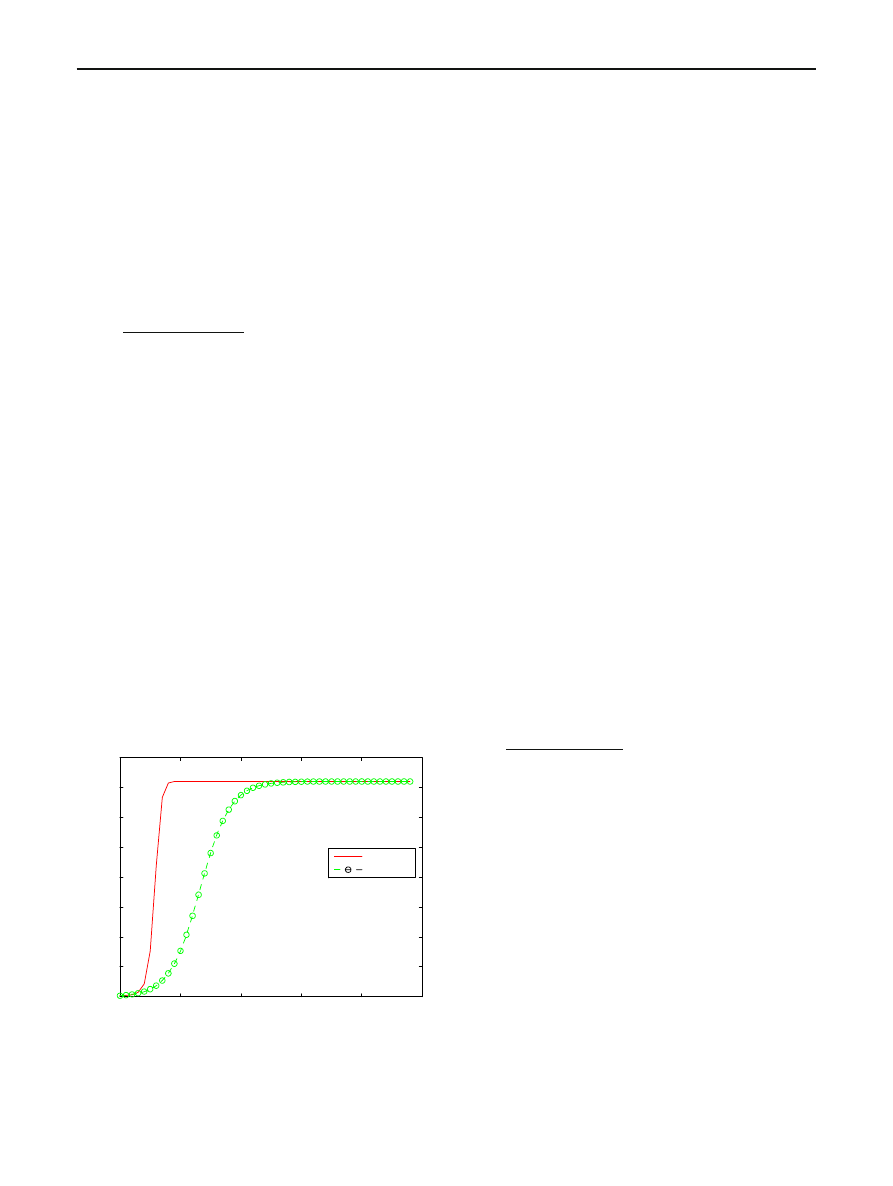
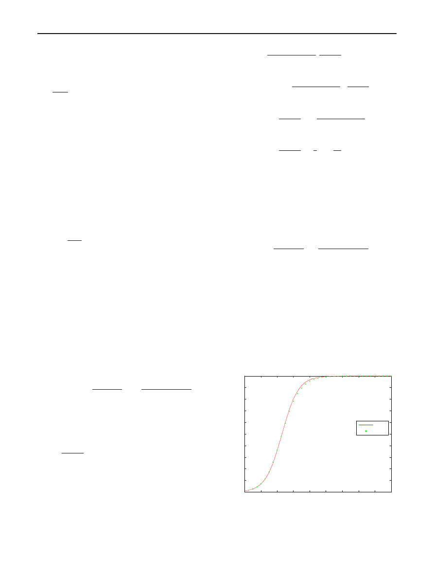
> 1 . For this choice of β(t), the NHRS

model reduces to

I

(t) =

N

1

+ ψ exp{−(βt)

K

}

.

(20)

Figure

1

gives a sketch of this I

(t) when N = 360,000,

I

0

= 1,780, β = 0.8, and K = 2. The other curve in Fig.

1

corresponds to the RCS model with the same values of N ,

I

0

, and

β.

It may be noted here that the model derived in Proposi-

tion

1

does not allow the so-called local preference scanning

[

15

]. Local preference scanning is a strategy in which an

infected host scans IP addresses close to its own address
with a higher probability than other IP addresses. However,
the assumption (iv) of Proposition

1

, namely that p

(t, t +

t) is the same for each pairing of susceptible hosts with
infected hosts, rules out local preference scanning. As seen
in the proof of Proposition

1

, this assumption, as well as the

other assumptions of Proposition

1

, are essential for the appli-

cability of the NHRS model. The flexibility of choosing a
time-dependent contact function does not translate into spa-
tial preference in scanning.

The rest of this paper provides a rigorous development

of further foundational aspects of the NHRS model and its

0

5

10

15

20

25

0

0.5

1

1.5

2

2.5

3

3.5

4

x10

5

Time: t

I(t)

I(t)

RCS model

Fig. 1 Expected number of hosts infected against time since start of
epidemic

special case of the RCS model. Clearly, the NHRS model is
only one of the many possible generalizations of the RCS
model. Several generalizations of the RCS model are avail-
able in the literature even though their discussions have not
been concerned with questions of the kind we deal with in
this paper. Motivated by the classical Kermack-Mckendrick
model of theory of epidemics, Zou et al. [

14

] proposed an

internet worm model called the two-factor worm model. This
model takes into account the measures to counter the spread
of randomly scanning worms through removal of infectious
and susceptible hosts. Serazzi and Zanero [

12

] proposed a

compartment-based model based on the macro view of the
Internet as the interconnection of a number of Autonomous
Systems (AS). It models the behavior of the worm in the intra-
AS propagation while assuming that the inter-AS spread fol-
low RCS models. Chen et al. [

1

] developed an active worm

propagation (AAWP) model which improves on the classical
Kephart–White epidemiological model of computer viruses.
This model assumes random scanning, treats time as discrete
and employs continuous state deterministic approximation.
We refer to [

1

,

12

,

14

] for additional details about these three

generalizations of the RCS model. Without going into further
details, we note that the classical epidemiological models for
disease progression provide many possible ways of modeling
worm propagation.

2.2 Fitting the nonhomogeneous random scanning model

If we introduce the function

µ(t) = (1/t)

t

0

β(u)du t > 0,

then the NHRS formula (

4

) can be written as

I

(t) =

N

1

+ ψ exp{−tµ(t)}

.

(21)

The function

µ(t) can be interpreted as the average contact

rate over the interval

[0, t]. If N, the total number of hosts

in the network under consideration, and I

0

, the number of

hosts infected at the beginning of the worm epidemic, are
known then fitting the NHRS model amounts to estimating
the average contact rate function

µ(t). For this purpose, we

propose the approach given below.

It will be assumed that the available data consists of N ,

I

0

, and n pairs

(t

i

, X(t

i

)) where X(t

i

) denotes the observed

number of hosts infected during

[0, t

i

], 0 ≤ t

1

< t

2

<

· · · < t

n

. As we will see in an illustrative example later, n

need not be large although a large value of n would give a
better estimate of the average contact rate function

µ(t).

Since I

(t) = E{X(t)}, we will take ˆI(t

i

) = X(t

i

) as out

estimate of I

(t

i

), i = 1, 2, . . . , n. Our fitting procedure is as

follows:

123

36

E. Kirmani, C. S. Hood

Step 1. For each i

= 1, 2, . . . , n, compute

µ

i

=

1

t

i

ln

(N − I

0

) ˆI(t

i

)

(N − ˆI(t

i

))I

0

.

(22)

Step 2. Obtain a smooth function

ˆµ(t) which passes

through the points

(t

i

, µ

i

), i = 1, 2, . . . , n; i.e.,

ˆµ(t

i

) = µ

i

,

and take

ˆµ(t) as an estimate of the average contact rate func-

tion

µ(t). Estimate I (t)

ˆI(t) =

N

1

+ ψ exp{−t ˆµ(t)}

.

(23)

The curve ˆ

I

(t) is then the NHRS fit to the observed data

(t

i

, X(t

i

)), i = 1, 2, . . . , n.

The crucial step in the above procedure is, of course,

the smoothing part of step2. Piecewise polynomial functions
such as splines are popular choices for such smooth functions.
The MATLAB function pchip finds a piecewise cubic Her-
mite interpolating polynomial which preserves the shape and
monotonicity of the underlying data. The following example
illustrates how our procedure can be applied in practice.

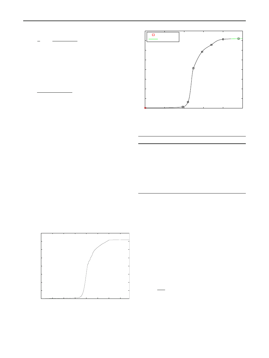
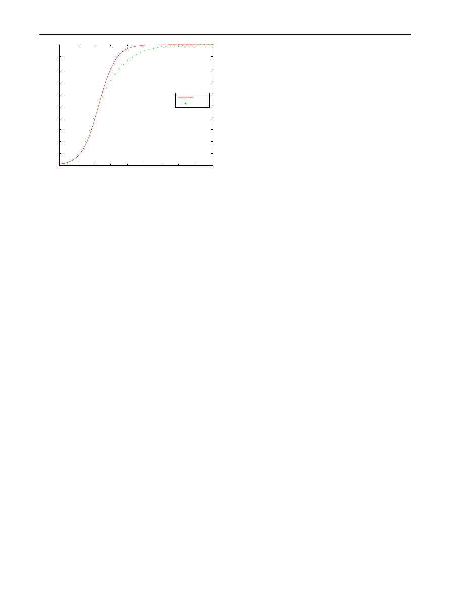
Example 1 We will use the data on the CRv2 epidemic given
in [

7

,

8

]. Figure

2

(taken from [

7

]) shows the number of dis-

tinct IP addresses infected (during the stated 24 h time span)
as found on merging three network telescope datasets.
According to this figure, more than 359,000 unique IP
addresses were detected as victims of CRv2 during the time
period t

= 0 to t = 24. Here, t is in hours and t = 0 corre-

sponds to midnight (UTC) of July 19, 2001.

For purpose of illustration, we will ignore the detailed

information given by Fig.

2

and use instead the approximate

numbers given in Table

1

. We have obtained these numbers

0

50000

100000

150000

200000

250000

300000

350000

400000

00:00
07/19

04:00

08:00

12:00

16:00

20:00

00:00
07/20

04:00

infected hosts

time (UTC)

Fig. 2 Number of unique IP addresses infected by CRv2 on July 19,
2001 [From [

7

]]

0

5

10

15

20

25

0

0.5

1

1.5

2

2.5

3

3.5

4

x10

5

Observed data

Fitted model

Fig. 3 Fit of NHRS model to the data of Table

1

Table 1 Estimated number of unique IP addresses infected

Row

t

Number of hosts infected during

[0, t]

1

0.0

1

,780

2

9.7

7

,140

3

11.0

32

,140

4

12.4

207

,150

5

14.6

292

,850

6

17.0

328

,570

7

20.0

357

,000

8

24.0

360

,000

by visual examination of Fig.

2

and make no claims of

accuracy.

Our procedure gives Fig.

3

as the fit of the NHRS model

to the data of Table

1

. We used the pchip interpolation func-

tion of MATLAB to find the smooth function of step 2 of our
procedure. The validity and potential of our approach are
clear.

2.3 Fitting the RCS model

The RCS model given in (

2

) is even easier to fit because it

assumes that the contact rate does not change with time. Let

Y

∗

t

= ln

N

I

(t)

− 1

.

(24)

Then, the RCS model holds with constant contact rate

β if,

and only if,

Y

∗

t

= ln ψ − βt

123

Analysis of a scanning model of worm propagation

37

where

ψ = (N − I

0

)/I

0

. Writing

Y

t

= ln

N

X

(t)

− 1

and noting that X

(t) is an estimate of I (t) suggests that

Y

t

= ln ψ − βt +

(25)

where

measures the random error. It follows that linear

regression or al least some parts of it can be applied here. In
particular, we can use the principle of least squares and those
of its features which do not require random error

to have

normal distribution. Assuming that N is known, and that the
observed data consists of n pairs

(t

i

, X(t

i

)), we propose the

following two step procedure for fitting the RCS model and
checking its accuracy.

Step 1. Let Y

i

= ln

N

X

(t

i

)

− 1

. Obtain the least-squares

regression line of Y on t from the n pairs

(t

i

, Y

i

). Take the

slope of this regression line as the estimate of the (constant)
contact rate

β.

Step 2. Do the usual analysis of residuals to see if the

model is appropriate.

Example 2 Most of the infections described in Fig.

2

occurred between 10:00 UTC and 20:00 UTC. It would be
interesting to see if this portion of the CRv2 epidemic could
possibly be explained by the RCS model. If so, the contact
rate

β during this period would be estimated by the slope

of the regression line of ln

((N/ X(t)) − 1) on t. Assuming

N

= 360,000, we implemented the proposed procedure for

the data given in rows 2–7 of Table

1

. The fitted regression

line has the equation

Y

= 10.711 − 0.790t

(26)

However, the plot of residuals against t is found to be cur-
vilinear, indicating that RCS model is not really suitable in
this situation.

3 Structure and simulation of NHRS and RCS models

The complete structure of an epidemic cannot be understood
by looking at the expected number of infected hosts alone.
It is also necessary to understand the behavior of the time
points at which the successive infections occur. For this pur-
pose, we need to know the probability distribution of the time
until infection for a host which was not infected at the start of
the epidemic. This distribution is given below for our NHRS
model and its special case the RCS model.

For convenience in writing, let

B

(t) =

t

0

β(u)du

so that the expected number of hosts infected during

[0, t] in

an NHRS epidemic is given by

I

(t) =

N

1

+ ψ exp{−B(t)}

.

where

ψ = (N − I

0

)/I

0

.

Proposition 2 Let T denote the time until infection (mea-
sured from t

= 0: the start of the epidemic) for a host which

was not infected at the start of the epidemic. If the worm
propagation in the network of N hosts follows the NHRS
model

d

dt

I

(t) = β(t)I (t)

I

−

I

(t)

N

then

P

(T ≤ t) =

1

− exp{−B(t)}

1

+ ψ exp{−B(t)}

, t ≥ 0,

(27)

where

ψ = (N − I

0

)/I

0

and I

0

= I (0) is the number of

hosts infected at t

= 0.

Proof For each initially uninfected host i (i

= 1, 2, . . . ,

N

− I

0

), let

C

i

(t) =

1

, if host i gets infected during (0, t]

0

, otherwise.

Then, each C

i

(t) has the same probability distribution with

E

{C

i

(t)} = P(C

i

(t) = 1)

= P(T ≤ t).

(28)

Writing X

(t) to denote the number of hosts infected during

[0, t], we have

X

(t) − I

0

=

N

−I

0

i

=1

C

i

(t)

(29)

so that

E

{X(t)} − I

0

=

N

−I

0

i

=1

E

{C

i

(t)}

= (N − I

0

)P(T ≤ t).

(30)

Therefore,

P

(T ≤ t) =

E

{X(t)} − I

0

N

− I

0

=

I

(t) − I

0

N

− I

0

=

1

N

− I

0

N

1

+ ψ exp{−B(t)}

− I

0

=

1

N

− I

0

N

− I

0

− I

0

ψ exp{−B(t)}

1

+ ψ exp{−B(t)}

=

1

N

−I

0

N

−I

0

−(N−I

0

) exp{−B(t)}

1

+ ψ exp{−B(t)}

=

1

− exp{−B(t)}

1

+ ψ exp{−B(t)}

.

(31)

123

38

E. Kirmani, C. S. Hood

The probability distribution of T in a RCS epidemic is

immediately obtained on putting B

(t) = βt in the above

proposition. The complete structure of the NHRS and RCS
epidemics can now be described. Let L

= N − I

0

denote the

number denote the number of hosts which were not infected
at the start of the epidemic. Further, let T

1

, T

2

, . . . , T

L

be

L mutually independent random variables such that each of

them has the same probability distribution as T . Suppose
that T

(1)

≤ T

(2)

≤ · · · ≤ T

(L)

is the ordered (in increasing

magnitude) arrangement of T

1

, T

2

, . . . , T

L

. Then, T

(1)

is the

time of occurrence (measured from the start of the epidemic)
of the first infection (excluding the ones which happened at
t

= 0), and T

(i)

the occurrence time of the i th infection. The

last host to be infected is infected at time point T

(L)

. The

importance of this description lies in the fact that later it will
help us to simulate worm propagation.

In the rest of this section we will focus on the RCS model.

3.1 Simulation of a RCS epidemic

It is crucial to be able to simulate worm propagation in order
to see the extent to which a specific realization of an epi-
demic may differ from the predictions of the model. How-
ever, as observed in [

10

], a comprehensive risk analysis of a

detection/defense strategy needs to consider the probability
distributions governing worm propagation. The impact of the
variability between successive infection times on the variabil-
ity in worm propagation cannot be captured efficiently unless
simulations are explicitly based on the probabilistic regime
underlying worm behavior. With this in view, we propose a
simulation procedure based on the probability distribution
of successive infection times. The following proposition is
important for our simulation procedure for the RCS worm
propagation.

Proposition 3 Let U be a random variable having the uni-

form distribution on the interval

(0, 1). Then

1

β

ln

1

+ψU

1

−U

has the same probability distribution as T .

Proof For all t

> 0,

P

1

β

ln

1

+ ψU

1

− U

≤ t

= P

U

≤

1

− exp(−βt)

1

+ ψ exp(−βt)

=

1

− exp(−βt)

1

+ ψ exp(−βt)

= P(T ≤ t)

(32)

where the second equality holds because P

(U ≤ u) = u for

all u

∈ (0, 1).

We now propose the following procedure for simulating

a RCS epidemic in a network of N hosts of which I

0

are

infected at the start of the epidemic at t

= 0. It would be suf-

ficient to simulate the times at which the remaining N

− I

0

hosts get infected.

Simulation procedure:
Step 1. Draw L

= N − I

0

numbers randomly (i.e., accord-

ing to the uniform distribution) from the interval

(0, 1). Let

U

1

, U

2

, . . . , U

L

denote the L numbers drawn.

Step 2. Sort U

1

, U

2

, . . . , U

L

to get U

(1)

, U

(2)

, . . . , U

(L)

with U

(1)

≤ U

(2)

≤ · · · ≤ U

(L)

.

Step 3. Compute T

(i)

=

1

β

ln

(

1

+ψU

(i)

1

−U

(i)

), i = 1, 2, . . . , L.

Then T

(i)

is the time point at which infection number i occurs.

The epidemic terminates (with all hosts infected) at time
point T

(L)

.

Step 4. For all t

> 0 and i = 1, 2, . . . , L; define

K

i

(t) =

1

, T

(i)

≤ t

0

, T

(i)

> t

Further, let

X

(0) = I

0

X

(t) = I

0

+

L

i

=1

K

i

(t), t > 0

(33)

Then, X

(t), t ≥ 0, is the path of the simulated RCS epidemic.

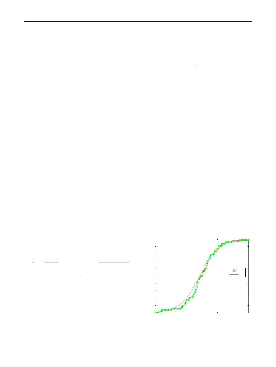
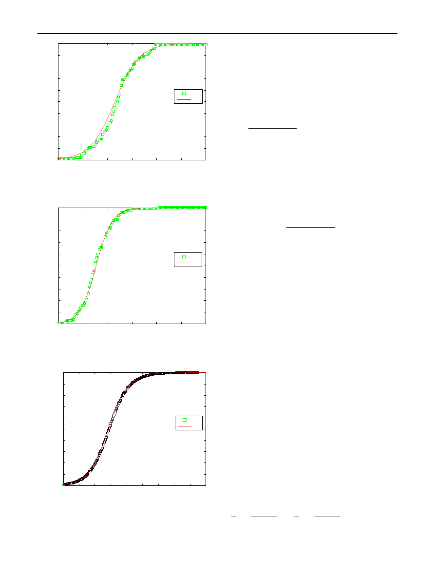
Figures

4

,

5

,

6

, and

7

show some realizations of the RCS

epidemic simulated according to the above procedure. In each
case, N , I

0

, and

β are shown for parametric choices indicated

under the figure. The solid line in each figure is the expected
path predicted by the corresponding RCS model.

To understand the RCS epidemic, we also need the proba-

bility distribution (not just the expected value) of the number
of hosts infected during the time period

[0, t]. When the num-

ber of hosts infected at t

= 0 (i.e., at the start of the epidemic)

is known, it is sufficient to find the probability distribution of
the number of hosts infected during

(0, t]. This distribution

is obtained below.

0

2

4

6

8

10

12

0

10

20

30

40

50

60

70

80

90

100

Time: t

Number of hosts infected

X(T)

I(t)

Fig. 4 Simulation of the RCS model for N

= 100, I

0

= 1, β = 0.8

123

Analysis of a scanning model of worm propagation

39

0

2

4

6

8

10

12

0

10

20

30

40

50

60

70

80

90

100

Time: t

Number of hosts infected

X(T)

I(t)

Fig. 5 Simulation of the RCS model for N

= 100, I

0

= 1, β = 1

0

2

4

6

8

10

12

0

10

20

30

40

50

60

70

80

90

100

Time: t

Number of hosts infected

X(T)

I(t)

Fig. 6 Simulation of the RCS model for N

= 100, I

0

= 1, β = 1.5

0

2

4

6

8

10

12

14

16

18

0

1000

2000

3000

4000

5000

6000

7000

8000

9000

10000

Time: t

Number of hosts infected

X(T)

I(t)

Fig. 7 Simulation of the RCS model for N

= 10,000, I

0

= 100,

β = 0.8

Proposition 4 Let Y

(t) = X(t) − I

0

so that Y

(t) denotes

the number of hosts infected during

(0, t]. If the RCS model

of worm propagation is applicable then, given I

0

, Y

(t) has

the binomial distribution

P

(Y (t) = y) =

L
y

{G(t)}

y

{1 − G(t)}

L

−y

where y

= 0, 1, . . . , L; L = N − I

0

, and

G

(t) =

1

− exp{−βt}

1

+ ψ exp{−βt}

t

≥ 0,

(34)

with

ψ = (N − I

0

)/I

0

.

Proof Let T

1

< T

2

< · · · < T

L

denote the times (mea-

sured from t

= 0: the start of the epidemic) at which the

L

= N −I

0

initially uninfected hosts become infected. Then,

as seen above, the L random variables T

1

, T

2

, . . . , T

L

behave

as the order statistics of a random sample of size L from a
population with distribution function

G

(t) ≡ P(T ≤ t) =

1

− exp{−βt}

1

+ ψ exp{−βt}

t

≥ 0.

(35)

It follows that

P

(T

i

≤ t) =

L

r

=i

L
y

{G(t)}

r

{1 − G(t)}

L

−r

for i

= 1, 2, . . . , L. For convenience in writing, let p =

G

(t). Then for n = 0, 1, . . . , L,

P

(Y (t) = n) = P(Y (t) ≥ n) − P(Y (t) ≥ n + 1)

= P(at least n hosts are infected during (0, t])

−P(at least n+1 hosts are infected during (0, t])

= P(T

n

≤ t) − P(T

n

+1

≤ t)

=

L

r

=n

L

r

p

r

(1−p)

L

−r

−

L

r

=n+1

L

r

p

r

(1−p)

L

−r

=

L

n

p

n

(1 − p)

L

−n

, p = G(t).

(36)

4 Confidence interval for contact rate and impact

of prior distribution on the RCS model

A confidence interval for unknown

β can be obtained with

the help of the above proposition. If Y

(t

0

) is the number of

hosts infected during an observation period

(0, t

0

] then an

approximately 100

(1 − α)% confidence interval for β is

1

t

0

ln

1

+ ψ ˆp

1

1

− ˆp

1

,

1

t

0

ln

1

+ ψ ˆp

2

1

− ˆp

2

(37)

123

40

E. Kirmani, C. S. Hood

where

ˆp

1

= ˆp − z

α/2

{ ˆp(1 − ˆp)/L}

1

/2

,

ˆp

2

= ˆp + z

α/2

{ ˆp(1 − ˆp)/L}

1

/2

,

(38)

ˆp =

Y

(t

0

)

L

,

L

= N − I

0

ψ = (N − I

0

)/I

0

,

and z

α/2

is the 100

(1 − (α/2))th percentile of the standard

normal distribution.

Even though the actual value of

β may not be known, there

may be some prior information or judgement about the range
in which

β may lie. In case such information is available, it

should be used in the study of worm propagation. We show
below the proper approach in such situations.

Suppose the prior information or judgement suggests that

the actual value of

β is in the interval [θ

1

, θ

2

] where θ

1

, θ

2

are specified. If all values in this interval are deemed equally
credible then this prior information can be described by the
probability density function (pdf)

h

(β) =

1

θ

2

−θ

1

, θ

1

≤ β ≤ θ

2

0

,

otherwise

.

(39)

In effect, we then think of the actual value of

β as the realized

value of a random variable B whose pdf is the uniform distri-
bution over

[θ

1

, θ

2

]. This, of course, is the Bayesian approach

so common in scientific investigations. In the context of the
number of hosts infected during

[0, t] under the RCS model,

the implication is as follows.

Proposition 5 Given a set of N hosts, let X

(t) be the number

of hosts infected during the time period

[0, t] with X(0) = I

0

.

Suppose that (i) the RCS model is applicable but the exact
value of

β is unknown, and (ii) the prior distribution for β is

the uniform distribution on

[θ

1

, θ

2

]. Then

E

{X(t)} = N −

N

t

(θ

2

− θ

1

)

ln

1

+ ψ exp(−tθ

1

)

1

+ ψ exp(−tθ

2

)

(40)

Proof Let B be a random variable having the uniform distri-
bution on

[θ

1

, θ

2

]. Then, B has pdf

h

(β) =

1

θ

2

− θ

1

, θ

1

≤ β ≤ θ

2

and

E

{X(t)} = E[E{X(t)|B}]

=

θ

2

θ

1

E

{X(t)|B = β}h(β)dβ

=

θ

2

θ

1

N

1

+ ψ exp(−βt)

.

1

θ

2

− θ

1

d

β

= N

θ

2

θ

1

1

−

ψ exp(−βt)

1

+ ψ exp(−βt)

1

θ

2

− θ

1

d

β

= N −

N

θ

2

− θ

1

θ

2

θ

1

ψ exp(−βt)

1

+ ψ exp(−βt)

d

β

= N −

N

θ

2

− θ

1

1

t

b

a

d y

y

(41)

where

a

= 1 + ψ exp(−tθ

2

)

and

b

= 1 + ψ exp(−tθ

1

).

It follows that

E

{X(t)} = N −

N

t

(θ

2

− θ

1

)

ln

1

+ ψ exp(−tθ

1

)

1

+ ψ exp(−tθ

2

)

As an illustration of the importance and implications of

incorporating prior information about

β, suppose β is

assumed to be 1 when, in fact, all that can be justified is
that

β lies somewhere in an interval containing 1. The dotted

curves in Figs.

8

and

9

give the expected number of hosts

infected when the prior distribution of

β is uniform on the

intervals [0.8, 1.2] and [0.5, 1.5], respectively. In both figures,

N

= 100, I

0

= 1, and the solid curves gives the expected

number of hosts infected when

β actually equals1.

0

2

4

6

8

10

12

14

16

18

0

10

20

30

40

50

60

70

80

90

100

Time since the beginning of epidemic

Expected number of hosts infected

I(t)

E(X(t))

Fig. 8 Prior distribution is uniform on [0.8, 1.2]

123

Analysis of a scanning model of worm propagation

41

0

2

4

6

8

10

12

14

16

18

0

10

20

30

40

50

60

70

80

90

100

Time since the beginning of epidemic

Expected number of hosts infected

I(t)

E(X(t))

Fig. 9 Prior distribution is uniform on [0.5, 1.5]

5 Conclusion and future work

First of all, we gave a model for taking into account the fact
that in practice a worm’s scanning rate varies during the dura-
tion of the epidemic. Our NHRS model thus captures a much
larger class of worm propagation than the well-known RCS
model. This generality has been achieved without sacrific-
ing the intrinsic simplicity of the RCS model. The method
given by us to estimate the average contact rate function in
the NHRS model is practical and convenient for fitting the
NHRS model to observed data. We illustrated our method by
fitting NHRS model to the number of distinct IP addresses
infected during the first twenty four hours of the epidemic
caused by version 2 of the Code Red worm. We also gave a
linear regression approach to fitting the RCS model. As seen
in Sect.

2

, the CRv2 considered there is perfectly described

by a NHRS model while the RCS model is found to be unsuit-
able. The probability distribution of the time until infection
(for an initially uninfected host) derived for the NHRS model,
in Sect.

3

, enabled us to describe the structure of the NHRS

and RCS epidemics in terms of the times at which succes-
sive infections occurred. As a further application, we used
this probability distribution to illustrate simulation of RCS
epidemic. We also gave a confidence interval for the unknown
contact rate of the RCS model. Finally, we demonstrated how
the expected number of infected hosts in a RCS epidemic is
affected if the contact rate is uniformly distributed over a
specified interval. This Bayesian approach enables us to see
the effect of uncertainty about the contact rate on the predic-
tions of the RCS model.

The analysis carried out in this paper illuminated a number

of aspects of random scanning models of worm propagation
and led to several useful procedures. In addition to obtaining
the much more widely applicable NHRS model, we laid bare
the entire probabilistic regime governing RCS epidemics. As

mentioned earlier in Sect.

3.1

, it is only through the knowl-

edge of the probability distributions underlying model behav-
ior that a comprehensive risk analysis of defense strategies
can be undertaken. It may be added here that the NHRS model
can be extended to describe recovery, patching and immu-
nization of systems. Indeed, we have developed an imper-
fect protection-imperfect recovery (IMP-IMR) model which
takes into account possibilities such as (i) preventive steps,
not necessarily error proof, may be in place, (ii) immunity
obtained by preventive steps may be temporary, and (iii) dis-
infection, recovery action, or some other strategy, not nec-
essarily error-proof, is being used to contain the epidemic.
We are currently investigating the probability distributions
associated with our IMP-IMR model. We believe that anal-
ysis similar to those in the present paper are required for
IMP-IMR as well as other worm propagation models.

Acknowledgments

We thank Dr. Eric Filiol, the editor of the Journal

in Computer Virology, and the anonymous reviewers for their helpful
comments.

References

1. Chen, Z., Gao, L., Kwiat, K.: Modeling the spread of active

worms. In: Bauer, F. (ed.) IEEE INFOCOM 2003: The Confer-
ence on Computer Communications: 22nd Annual Joint Confer-
ence of the IEEE Computer and Communications Societies, Vol. 3,
pp. 1890–1900, IEEE Operations Center, New Jersey (2003)

2. Cisco technical notes: Dealing with mallocfail and high CPU uti-

lization resulting from the “Code Red” worm. Cisco Systems, Inc.

http://www.cisco.com/warp/public/63/ts_codered_worm.shtml

3. Cisco security advisory: “Code Red” worm—customer impact.

Cisco

Systems,

Inc.

http://www.cisco.com/warp/public/707/

cisco-code-red-worm-pub.shtml

4. Kephart, J.O., White, S.R.: Measuring and modeling computer

virus prevalence. In: Proceedings of the 1993 IEEE Computer Soci-
ety Symposium on Research in Security and Privacy, pp. 2–15.
IEEE Computer Society Press, California (1993)

5. Kephart, J.O., White, S.R., Chess, D.M.: Computers and epidemi-

ology. IEEE Spectr 30(5), 20–26 (1993)

6. Lee, W., Wang, C., Dagon, D.: Botnet Detection, countering

the largest security threat. Springer Science+Business Media,
LLC, New York (2008)

7. Moore, D., Shannon, C., Brown, J.: Code-red: a case study on the

spread and victims of an internet worm. In: Proceedings of the 2nd
Internet Measurement Workshop, pp. 273–284. ACM Press, New
York (2002)

8. Moore,

D.,

Shannon,

C.:

The

spread

of

the

code-red

worm (CRv2). CAIDA.

http://www.caida.org/analysis/security/

code-red/coderedv2_analysis.xml

9. Moore, D., Shannon, C., Voelker, G., Savage, S.: Internet quaran-

tine: requirements for containing self-propagating code. In: Bau-
er, F. (ed.) IEEE INFOCOM 2003: The Conference on Computer
Communications: 22nd Annual Joint Conference of the IEEE Com-
puter and Communications Societies, pp. 1901–1910, IEEE Oper-
ations Center, New Jersey (2003)

10. Nicol, D.M.: The impact of stochastic variance on worm propaga-

tion and detection. In: Proceedings of the 2006 ACM Workshop on
Rapid Malcode (WORM’06), pp. 57–63, ACM Press, New York
(2006)

123

42

E. Kirmani, C. S. Hood

11. Qing, S., Wen, W.: A survey and trends on internet worms. Comput

Secur 24, 334–346 (2005)

12. Serrazi, G., Zanero, S.: Computer virus propagation models.

In: Calzarossa, M.C., Gelenbe, E. (eds.) MASCOTS 2003: Tuto-
rials of the 11th IEEE/ACM International Symposium on Model-
ing, Analysis and Simulation of Computer and Telecommunication
Systems. Springer, Heidelberg (2003)

13. Staniford, S., Paxson, V., Weaver, N.: How to own the Internet

in your spare time. In: Proceedings of the 11th USENIX Secu-
rity Symposium, pp. 149–170. USENIX Association, California
(2002)

14. Zou, C.C., Gong, W., Towsley, D.: Code red worm propagation

modeling and analysis. In: Proceedings of the 9th ACM Confer-
ence on Computer and Communications Security, pp. 138–147,
ACM Press, New York (2002)

15. Zou, C.C., Towsley, D., Gong, W.: On the performance of internet

worm scanning strategies. Perfor Eval 63, 700–723 (2006)

123