Models for drying kinetics based on drying curves of slabs

Chemical Engineering and Processing 39 (2000) 53 – 68

W.J. Coumans *

Laboratory for Separation Processes and Transport Phenomena, Eindho

6en Uni6ersity of Technology, PO Box

513

5600

MB Eindho

6en, The Netherlands

Received 7 June 1999; accepted 28 June 1999

Abstract

An overview of approximate models for the drying kinetics is given, including lumped diffusion models, retreating front models

and the characteristic drying curve model. To keep this overview orderly, only drying bodies with a slab geometry and a constant
temperature are considered. The presented models enable — in a relatively simple way — the characterization and description of the
drying behavior. All model parameters are derived from drying curves of slabs. The methods given relate to porous and
non-porous materials. An attempt is being made to give a consistent presentation of these methods coming from different
literature sources, by using the same definitions, nomenclature and symbols for the model parameters involved. For a correct
analysis of the practical usefulness of the given methods more experimental data are needed. Some additional conclusions and
recommendations are given. © 2000 Elsevier Science S.A. All rights reserved.

Keywords

Drying curves; Drying kinetics; Short cut methods; Diffusion coefficient

www.elsevier.com/locate/cep

1. Introduction

The description and prediction of the drying kinetics

of a given material under given process conditions is
still a weakness in the modeling of drying processes.
Even now, in design and optimization of drying pro-
cesses, there is a great need for stable and reliable
models to quantify and predict drying rates and drying
times with a satisfying accuracy. Over the last decades
several approaches have been proposed about how to
deal with mass and heat transfer phenomena in materi-
als during a drying process.

Crank [1] gives an excellent overview of mass transfer

models based on Fickian diffusion. In his book analyt-
ical solutions of the diffusion equation are given for
several body geometries with many types of initial and
boundary conditions. Dudas and Vrentas [2] developed
the ‘free volume theory’ to describe diffusion coeffi-
cients in polymer/solvent systems over a wide range of
concentrations and temperatures. In numerous in-
stances unsteady state diffusion in concentrated poly-

mer solutions can not be described by classical diffusion
theories. This non-Fickian diffusion behavior is associ-
ated with the slow relaxation of large macromolecular
chains. It is obvious that during a drying process the
overall volume of the polymer/solvent system will
change. For rigid materials, in which a porous structure
will be built up during drying, Whitaker [3] has intro-
duced the ‘volume averaging method’. This method
takes into account several mechanisms for mass and
heat transfer, viz. liquid flow due to capillary forces,
vapor diffusion in a partially saturated porous struc-
ture, ‘bound’ moisture diffusion, internal evaporation
of moisture and heat transfer by convection and con-
duction. The ‘free volume theory’ for homogeneous
amorphous systems and the ‘volume averaging theory’
for porous materials have a strong physical basis, and
require quite a number of model parameters to be
found experimentally. These theories are rather labori-
ous, require a good laboratory infrastructure and — in
many cases — are not easy to use in practice. For this
reason approximate models have been proposed, for
which the model parameters can be evaluated relatively
simply from drying curves of slabs.

Generally, in drying processes internal heat transfer

occurs much faster than internal mass transfer, which

Dedicated to Prof em. Dr.-Ing. E.-U. Schlu¨nder on the occasion

of his 70th birthday.

* Tel.: + 31-40-247-3720; fax: + 31-40-243-9303.
E-mail address

w.j.coumans@tue.nl (W.J. Coumans)

PII: S 0 2 5 5 - 2 7 0 1 ( 9 9 ) 0 0 0 8 4 - 7

W.J. Coumans

Chemical Engineering and Processing

39 (2000) 53 – 68

means that in most cases a uniform temperature of the
drying material may be assumed. Then temperature
histories can be obtained in a straightforward manner
from a macroscopic non-stationary or quasi-stationary
enthalpy balance over the drying material. With respect
to the internal mass transfer it appears to be much
more complicated to develop a reliable and manageable
description. This is exactly the focus point of the ap-
proximate models. Unfortunately, for the time being
there does not exist a clear view as far as the practical
usefulness and the reliability of these methods are con-
cerned. For this reason, an attempt is being made in
this paper to present a consistent overview of these
approximate models and to draw some conclusions.
‘Consistent’ means that all models will be presented
here with the same definitions, nomenclature and sym-
bols for the parameters involved. This facilitates a
comparison of these models.

Some general limitations should be mentioned be-

forehand. Only the isothermal convective drying pro-
cess of slabs is considered and the drying curves behave
‘normally’, which means that there is neither a maxi-
mum nor a minimum. The presented models can be
classified according to the materials they are supposed
to serve:

Models for non-porous or

‘

pseudo

’

continuum materi-

als. These type of materials are considered to be
homogeneous, there are no-phase separations (e.g.
crystal formation), no formation of cracks, and vol-
ume shrinkage is ideal and takes place perpendicu-
larly to the slab surface only (1-D shrinkage). This
means that slab thickness is supposed to be much
smaller than the surface dimensions, e.g. liquid foods,
carbohydrate solutions, etc.
Models for porous, non-shrinking materials. These
materials are heterogeneous and they may be hygro-
scopic or non-hygroscopic, e.g. bricks, unglazen alu-
minum, etc.

2. Some basic theory on drying

To provide a complete and consistent overview of

drying kinetics it is inevitable to start with a brief
introduction of some basic theory on drying. More
details can be found in textbooks on drying [4,5] and
diffusion [1]. It is very important to establish whether a
drying process is controlled by external and/or internal
transport phenomena. The sorption isotherm and the
successively occurring drying stages play in many mod-
els a decisive role. This will be explained in some more
detail now.

. Sorption isotherms and Mollier charts

The relative humidity of the air (or any other drying

gas) is defined as the ratio of the actual vapor pressure
P

and the saturation vapor pressure P

v, sat

at the same

temperature T. At equilibrium the chemical potentials
of the moisture in the material and in the air are equal.
In other words, the moisture activity a

in the material

equals the relative humidity (RH) of the air, thus:

= RH =

v, sat

(T)

(1)

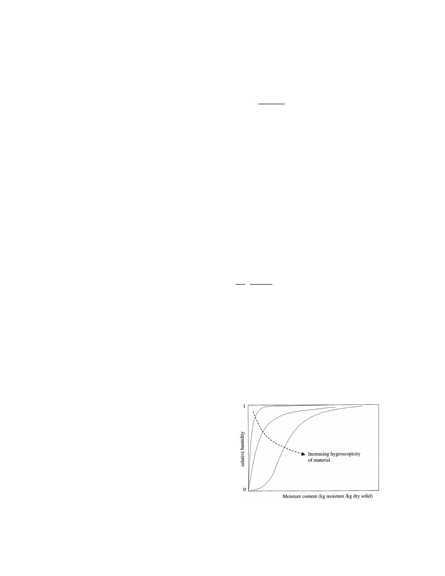
The equilibrium relationship between the averaged

moisture content, u¯, of the material (kg moisture/kg dry
solid) and the relative humidity (RH) of the surround-
ing air at a given temperature is called the sorption
isotherm (Fig. 1). This relationship indicates which air
condition(s) are needed to arrive at a given and desired
final moisture content of the product. The lower the
desired moisture content the lower the RH of the
drying air should be. In many drying models the sorp-
tion isotherm emerges in the boundary condition, be-
cause at the interface between the drying body and the
surrounding air a local thermodynamic equilibrium is
assumed.

At a given RH and a given temperature of the air the

actual vapor pressure P

follows directly from Eq. (1);

subsequently, at a given total pressure P

the absolute

air humidity Y can be obtained from:

Y =

− P

(2)

where M

and M

are respectively the molecular

weights of vapor and drying gas. In the case of water
vapor and air this ratio of molecular weights is 0.622.

The state of unsaturated, saturated and oversatu-

rated humid air, defined by P

, T and Y, is often

represented graphically in so-called Mollier charts.
Though these charts are basically enthalpy – humidity
diagrams at a given total pressure, they are often shown
as pseudo temperature – humidity charts (thus T – Y

Fig. 1. Typical sorption isotherms for materials with different degrees
of hygroscopicity.

W.J. Coumans

Chemical Engineering and Processing

39 (2000) 53 – 68

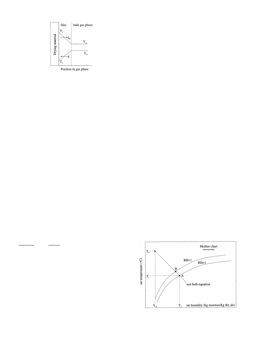
Fig. 2. Boundary layer near interface of drying material and air.

that the sorption-isotherm comes into the picture again.
If the equilibrium RH equals 1 (‘free moisture’), the
conditions at the interface are the so-called ‘wet-bulb
conditions’ and it is for this reason that Eq. (6) is also
often referred to as the ‘wet-bulb equation’.

. Constant rate period

(

CRP

)

Usually at the initial moisture content of the material

the RH equals 1. From the intersection of the wet-bulb
equation and where the RH is equal to 1 line in the
Mollier-diagram, the interface conditions (u

, T

) are

found (see Fig. 3). Though the interface moisture con-
tent of the material (u

) starts to decrease from the

beginning, the sorption isotherm indicates that the equi-
librium RH will remain constant or nearly constant
during a certain period. This means that under constant
air conditions the interface conditions will also remain
constant. Because the driving force for drying (Y

– Y

)

remains constant, a constant drying flux (kg/m

s) will

be observed. For materials with a constant exchange
area (slabs, non-shrinking materials) this also leads to a
constant drying rate (kg/s). Therefore this drying stage
is usually called the ‘constant rate period’ (CRP). The
drying process is controlled by external conditions as
long as the drying flux depends linearly on the mass
transfer coefficient k, according to Eq. (4). This is fully
true for the CRP. Also typical for this period is that the
moisture concentration profiles are strongly dependent
on the initial moisture content and the initial drying
rate.

For porous materials the initial drying rate may

remain constant over a wide range of moisture con-
tents. It is often observed that the CRP ends at a
surprisingly low average moisture content (called the
‘critical moisture content’, u¯

), e.g. less than 30% of the

pore saturation degree. At this level of moisture content
it is unlikely that the surface of the material will still be
completely wetted. Schlu¨nder [6] gives an interesting
analysis on this observation, explaining that under cer-
tain conditions partially wetted surfaces can maintain a
constant drying rate.

charts at a given P

). Nowadays, graphical representa-

tions of humid air conditions are gradually pushed
aside by user-friendly computer programs.

. Drying stages

The drying process is induced by air with a suffi-

ciently low RH (see Fig. 2). In an adiabatic convective
drying processes the energy for the moisture evapora-
tion has to be delivered by the hot air, which means
that the temperature of the drying material (‘wet-bulb
temperature’) will be lower than the temperature of the
air (‘dry-bulb temperature’).

In a stationary situation the heat flux q from the air

to the surface of the material equals the evaporation
enthalpy required for the moisture vapor flux j

vap

= q

(3)

in which

vap

is the evaporation energy of the mois-

ture. In a linearized form the moisture flux is given by:

= k

r¦

· (Y

− Y

)

(4)

and the heat flux by

q =

a · (T

− T

)

(5)

in which k is the mass transfer coefficient,

a the heat

transfer coefficient,

is the density of the humid air.

Substitution of Eqs. (4) and (5) into Eq. (3) gives:

− T

− Y

= − L

vap

p,a

where

L = Le

− 2/3

(6)

in which c

p,a

is the specific heat of the humid air and

is the psychrometric ratio. This ratio

L depends on the

transfer coefficients for mass (k) and heat (

a) and the

physical properties of the gas/vapor mixture. In case
the Chilton – Colburn analogy between heat and mass
transfer applies, the psychrometric ratio depends only
on the Lewis number of the gas phase. Because locally
at the interface an equilibrium condition may be as-
sumed, it holds that Y

also corresponds with the

equilibrium vapor pressure at temperature T

. In other

words, the interface conditions (Y

, T

) also depend on

the equilibrium RH at the boundary; it is at this point

Fig. 3. Mollier-diagram and wet bulb equation.

W.J. Coumans

Chemical Engineering and Processing

39 (2000) 53 – 68

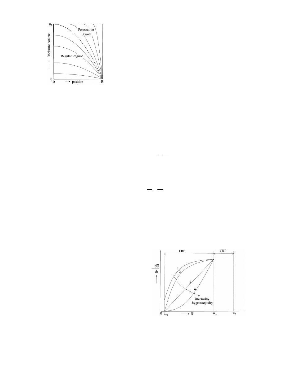
Fig. 4. Moisture profiles and drying stages (zero boundary concentra-
tion).

behavior in this period can be fully seen as a charac-
teristic of the material.

Though similar sub-stages may occur during the

CRP, they are not considered here.

3. Models for drying kinetics

Drying kinetics are generally characterized experi-

mentally by measuring the weight of a sample during
drying as a function of time. Drying curves may be
represented in different ways: averaged moisture con-
tent versus time (u¯ vs. t), drying rate versus time (du¯/dt
vs. t) or, as is done mostly, drying rate versus averaged
moisture content (du¯/dt vs. u¯).

Because drying times are inversely proportional to

drying rates, it is very important to have clear and
accurate representations at low drying rates (e.g. curve
4 in Fig. 5). In such cases a logarithmic scale for the
drying rate axis is preferred.

From a mass balance over the drying material the

following relationship for the drying flux j

is obtained:

= −

du¯

(7)

where M

is the mass of solid in the sample and A is the

mass exchange area of the sample. By combining Eqs.
(4) and (7):

−

du¯

· k

r¦

− Y

)

(8)

The CRP is fully determined by the external drying

conditions and the drying rate during this period can be
described with Eq. (8), where Y

is taken at the wet-

bulb conditions as is shown in Section 2.2.

Eq. (8) also holds for the FRP, however in general

the question now is: how to know the interface condi-
tions? Moreover, in case of a strong internal transport
limitation the interface moisture concentration will tend

. Falling rate period

(

FRP

)

After some time X

will reach some critical value,

where the sorption isotherm indicates that the equi-
librium RH will be significantly smaller than 1. The
intersection point (A in Fig. 3) shifts along the wet-bulb
equation (e.g. towards point B) and two important
effects can be observed:

the interface temperature starts to increase;

the driving force for drying starts to decrease.

This drying stage is called the falling rate period

(FRP). During this period an increase of the mass
transfer coefficient k leads to a quicker decrease of the
interface moisture content and thus also a lower inter-
face air humidity Y

. The effect of a higher value for k

is thus partially compensated by a decrease of the
driving force (Y

– Y

); now an internal diffusion resis-

tance in the drying material increasingly controls the
speed of the drying process. Soon the surface moisture
content will be close to the equilibrium value and a
constant boundary concentration will be obtained.

. Substages PP and RR. Up to now, it was rather

difficult to develop consistent, predictive, physically
sound and manageable models for the description of
internally controlled drying processes. In Section 3
some possible approaches will be given. In order to
obtain a good understanding of some of these ap-
proaches it is imperative to be aware of the two possi-
ble substages of the FRP with constant boundary
concentration (Fig. 4):

1. Penetration period (PP): during this drying stage the

moisture concentration profiles are still penetrating
towards the center of the material; the center mois-
ture concentration u

has not changed yet and the

moisture profiles are strongly dependent on the ini-
tial moisture content.

2. Regular regime (RR): the center moisture concentra-

tion is now clearly lower than its initial value; the
moisture concentration profile has become fully in-
dependent of the initial drying conditions, viz. initial
moisture content and initial drying rate. The drying

Fig. 5. Drying curves for materials with different degrees of hygro-
scopicity, e.g. curve 1 relates to a non-hygroscopic material, curve 4
to a high hygroscopic material.

W.J. Coumans

Chemical Engineering and Processing

39 (2000) 53 – 68

to the equilibrium value and the driving force becomes
very small (Y

– Y

0) and Eq. (8) becomes too inac-

curate. In the next section an attempt will be made to
explain the essentials of the following models for the
FRP:

General models:

Equilibrium drying model;

Characteristic drying curve.

Lumped diffusion models:

Constant diffusion coefficient;

Method of weighted averaged diffusion coefficients;

Power law diffusion;

Regular regime analysis or Schoeber’s approach;

Similarity of moisture profiles method;

Flux ratio method;

Rigorous numerical method.

Retreating front models:

Uniformly retreating moisture front model (URMF);

Method of Yoshida et al.

Some of these models also enable the evaluation of

moisture dependent diffusivities from experimental dry-
ing curves of slabs.

. General models

. Equilibrium drying model

At sufficiently low drying rates the drying material

will be close to equilibrium with the drying air at any
moment. Because under these drying conditions there is
no internal transport limitation (Biot number ap-
proaches zero) the moisture concentration profiles will
be nearly flat. In this marginal case the (local) interface
moisture content u

equals the averaged moisture con-

tent u¯, and the equilibrium RH at the interface follows
directly from the sorption isotherm at u

= u¯. The dry-

ing kinetics simply follow from Eq. (8). Next the value
for Y

in Eq. (8) can simply be found in the Mollier

chart at the intersection point of the wet bulb equation
and the equilibrium RH curve (see Fig. 3). In this
simple model the hygroscopic properties of the material
are thus taken into account.

. Characteristic drying cur

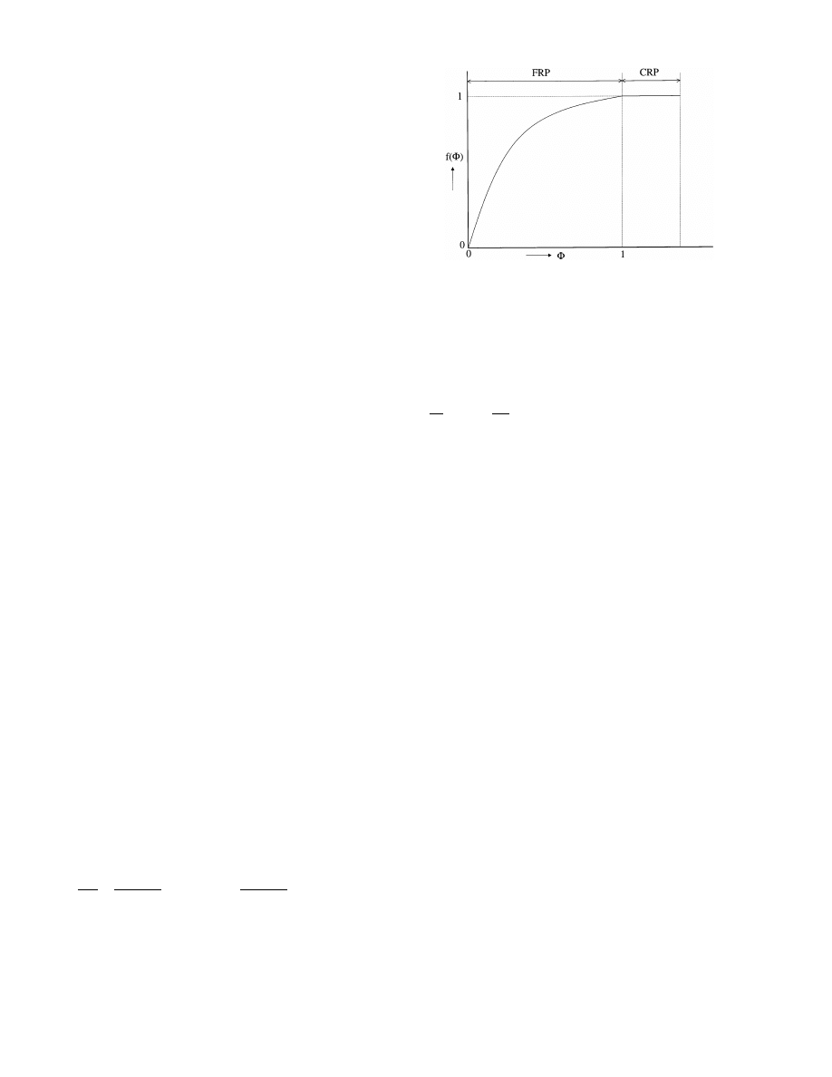
In certain cases the principle of the characteristic

drying curve (CDC) may apply [7 – 9] (Fig. 6). A crucial
parameter in this method is the so-called ‘critical mois-
ture content’, u¯

, defined as the averaged moisture

content where the CRP ends and the FRP starts. The
following normalization is usually applied to the exper-
imental data:

f =

m, 0

du¯/dt

(du¯/dt)

and

F =

u¯ − u

u¯

− u

(9)

where u

is the moisture content at equilibrium; for

slabs it is assumed that the surface area does not
change. The relationship between f and

F is by defini-

tion the CDC, thus:

Fig. 6. Characteristic drying curve.

CRP

f = 1

for

FRP

f = f(F)

for

(10)

By applying Eq. (8) the drying rate can be given

explicitly by:

−

du¯

= f(F) ·

· k

r¦

i, wet

− Y

)

(11)

By taking different drying conditions (temperature

and humidity of the drying air, initial moisture content,
mass transfer coefficient) the values for u

, u¯

and j

m, 0

will also change and thus different drying curves will be
obtained. However, if the CDC concept applies, the
function f(

F) should not change at all, or not too

much.

The critical moisture content, u¯

, is a space-averaged

moisture content at the moment that the CRP ends. At
‘high’ initial drying rates the removed moisture (u

−

u¯

) is inversely proportional to the drying rate, whereas

at ‘low’ initial drying rates this amount is linearly
dependent on the drying rate. The relationship between
the initial drying rate and the critical moisture content
is called the ‘critical point curve’, which has to be
determined experimentally.

The normalization procedure is ambiguous in the

case of a non-isothermal drying process and/or chang-
ing conditions of the drying air. Should the flux j

m, 0

taken at the initial conditions of the drying process or
at the conditions at any moment? And what should be
done in the event that no CRP exists?

The CDC approach has a weak theoretical basis. It

has been shown that for constant diffusivity processes
there is no single curve for a given material [9]. How-
ever, in cases where laboratory and industrial drying
conditions do not differ too much, the concept may be
used for interpolations and small extrapolations. In
cases where the concept works it may have great value
for practical design and optimization of drying pro-
cesses [9,10]. In many cases, where the CDC will not
work sufficiently well, other approaches are needed, e.g.
diffusion models. These models will now be discussed.

W.J. Coumans

Chemical Engineering and Processing

39 (2000) 53 – 68

. Lumped diffusion models

The mass transfer inside a body is described as a

diffusion process, so the drying kinetics here are charac-
terized by a moisture diffusion coefficient D. In this
approach all effects of different moisture transport
mechanisms in a complex porous or non-porous mate-
rial are lumped into a single parameter. In general, one
will observe that this apparent diffusion coefficient is
strongly dependent on moisture content and — to a
lesser degree — on temperature. In a drying process the
value of D may change several orders of magnitude,
due to its moisture concentration dependence.

. Diffusion equation for slabs

For a slab with thickness R and one-sided drying, the

following diffusion equation with IC and BC applies:

PDE:

IC:

t = 0

5r5R

BC1:

\0 r=0

= 0

BC2a:

r = R(t)

− D

= j

= k

r¦

· (Y

− Y

)

BC2b:

m, eq

(12)

where

is the local volume based moisture concen-

tration and r is the space coordinate. The above set of
equations applies both to non-shrinking and uni-direc-
tional shrinking slabs. For a non-shrinking slab R(t) =
R

at any time. In case of shrinkage ideal behavior is

assumed, which means that the volume decrease of the
slab equals the volume of the removed moisture, thus
no porous structure is being built up. For non-shrink-
ing and shrinking slabs the above set of Eqs. (12) can
be generalized according to the following dimensionless
form [14,17]:

PDE:

IC:

t=0 05f51 m=1

BC1:

t\0 f=0

= 0

BC2a:

f=1 −D

= F = Bi ·

r¦

− Y

)

BC2b:

(13)

The definitions of the dimensionless parameters are

given in Table 1. The given parameters for the ideal
shrinking slab are often referred to as solid-based
parameters. The flux parameter F is also often indicated
as the ‘drying intensity parameter’, because this
parameter enables to quantify more precisely the condi-

tions ‘high’ and ‘low’ drying rates (see also Section
3.2.2).

In the equations given in this table d

is a material

property representing the solid density of the pure and
pore free solid,

is the volume based solids concentra-

tion and R

is the so-called ‘solids radius’, which is the

final thickness of the slab after complete removal of the
moisture. In certain cases it might be more advanta-
geous to base a dimensionless moisture content on the
following definition

m − m

1 − m

(14)

which turns a constant boundary concentration m

into a zero boundary concentration.

The overall moisture balance (Eq. (7)) can now be

rewritten as:

F = −

(15)

In order to keep in touch with the experimental

reality we can rewrite this mass balance in several ways,
thereby introducing two more reduced flux parameters
F

and F

(see Table 2). In the given expressions we

have eliminated the often unknown diffusivity.

Because of the generalization of the diffusion equa-

tion, its solutions for non-shrinking and shrinking slabs
are exactly the same in terms of the defined dimension-
less parameters. This means for instance, that solutions
for non-shrinking slabs, as given in the next sections,
may also be applied to 1-D shrinking slabs, if in all
equations the following replacements are being made
(see Tables 1 and 2):

Table 1
Overview of dimensionless parameters

Parameter

Symbol

Non-shrinking

Ideally
shrinking

Moisture content

Space coordinate

r
0

R
0

r
0

Time

· t

Diffusion coefficient

Flux

·u

Biot number

· d

W.J. Coumans

Chemical Engineering and Processing

39 (2000) 53 – 68

Table 2
Overview of flux parameters and mass balance

Equation

Non-shrinking

Shrinking

Equation

no.

(16)

F =

= −

(17)

F =

· u

= −

= −R

(18)

(19)

= −d

= j

R = −R

r¯

= j

(21)

(20)

= −

du¯

= −d

du¯

[1,14]. The approximate solution for the drying rate is
given by:

F =

1 − m

(22)

By means of equations 16 and 18 this can be written as:

· D

1 − m

(23)

Where F

is a reduced flux parameter, which can easily

be evaluated from experimental drying data with equa-
tion 18. From a plot of F

versus 1/(1 − m

¯ ) the value

of D

can be obtained. From the above equations it can

also be derived that:

− R

· D

(24)

and a straightforward and less noisy plot of m

¯ versus

t will also yield the value of D

. Regular regime

(

)

. At sufficiently high drying

times the center moisture concentration has clearly
decreased. Now it is no longer possible anymore to
reconstruct the initial moisture concentration and the
initial drying rate from the moisture profiles. In other
words sooner or later the moisture profiles inside the
material become independent of the initial drying con-
ditions and all ‘switch on effects’ have stopped. The
analytical solution for the drying rate, based on a series
of exponential functions [1,14] is reduced for long peri-
ods to:

F =

· m

(25)

which can be reformulated as:

· D

· m

(26)

From a plot of F

versus m

¯ the value of D

can be

obtained. Alternatively it can be derived that

− R

d ln m

· D

(27)

and a straightforward plot of ln(m

¯ ) versus t will give

less noisy results.

The PP and RR drying curves are shown in Fig. 7. It

can be seen that these two extreme solutions are ap-
proaching each other at m

¯ = 0.5. To simplify the calcu-

lations a ‘short cut’ from the PP to RR drying curve is
proposed at this m

¯ -value. This will introduce only small

and acceptable errors (

B2%). The flux parameter at

this transition point is given by F

:1.25 (or F

1.25D

Note, that a graphic representation of a drying curve

according to F

versus m

¯ is independent of the initial

moisture content u

and the thickness R of the slab.

r¯

u¯o

and

For moisture dependent diffusion coefficients only in

some special cases analytical solutions for the diffusion
equation are known [1] but in general numerical meth-
ods are needed. In the next section we will first have a
closer look at the solutions in case of constant diffusion
coefficients. These solutions are often taken as a start-
ing point for obtaining approximate solutions for more
complicated situations.

. Constant diffusion coefficient

Simple diffusion models assume constant diffusion

coefficients (D = D

, thus D

= 1) and non-shrinking

bodies, which means that analytical solutions for the
above set of equations can be found in literature [1].
Let us now consider the situation with a zero boundary
concentration (BC2b: m

= 0), a condition which usu-

ally applies to the final drying stage, but which is also
closely obtained rather soon at low initial moisture
contents and/or high initial drying rates. Realize that it
is assumed now that the CRP is extremely short and
that from the beginning on the drying process is in the
FRP. We will not provide now the full analytical
solution, but we focus on the approximate solutions for
the two sub-stages:

. Penetration period

(

)

. At sufficiently short

drying times the moisture profiles have not yet pene-
trated to the center of the material. The drying slab
behaves like a semi-infinite thick body. An analytical
solution based on error functions can be developed

W.J. Coumans

Chemical Engineering and Processing

39 (2000) 53 – 68

As already stated earlier, most drying processes show

a CRP with an initial drying flux F

. From the exact

solution of the diffusion equation with zero boundary
conditions it appears that a good approximation of the
endpoint of the CRP follows from the intersection of
the CRP-line with the PP drying curve (at ‘high’ initial
drying rates) or with the RR drying curve (at ‘low’
initial drying rates). This means that the PP and RR
curves can also be seen as a good approximation of the
‘critical point curve’. The drying rate at the transition
point of PP and RR is given by F

= 1.25, a value that

is taken as the criterion to quantify ‘high’ and ‘low’
drying rates. It can be concluded, that if the initial
drying rate F

\1.25 the CRP will be followed by a PP

and a RR. On the other hand if F

B1.25 the CRP will

be succeeded directly by the RR and a PP will not be
observed.

Generally, moisture diffusion coefficients are highly

concentration dependent and shrinkage effects may not
always be ignored. Also for more realistic systems short
cut methods have been developed, departing from the
framework given above. This will be shown in the next
sections.

. Method of weighed a

6eraged diffusion coefficients

By means of Eqs. (23), (25) and (26) diffusion coeffi-

cients can be calculated from experimental drying data
F

versus m

¯ at any moment during the process. How-

ever, in case of moisture dependent diffusion coeffi-
cients, the values thus obtained should be interpreted as
some averaged values. In this approach it is proposed,
that the averaging takes place by using weighing factors
based on the moisture distribution in the slab [1,11].
For zero boundary concentration the averaging rules
found by Yamamoto et al. [11] are given by:

· D

(

1 − m

with

(

= q

(1 − m)

q − 1

D dm

(28)

and

· D

(

· m

(

p − 1

D dm

(29)

For several types of concentration dependent diffu-

sion coefficients it appears that p = 1.40 and q = 1.85.
As can be seen from Eq. (28) the value of D

(

takes on

a constant value (!), which only depends on the rela-
tionship between D and m. It has been shown analyti-
cally by Sano et al. [21] via a Boltzmann transformation
of the diffusion equation, that irrespective of the rela-
tionship D = D(m), the following property holds during
the PP:

(1 − m

¯ ) = constant

(30)

For slabs the value of this constant only depends on

the relationship D = D(m).

The diffusion coefficient D as a function of m can be

found via differential form of Eq. (29):

D =

p · m

d(D

(

· m

)

m = m

(31)

The consistency of this method can be verified by

using the obtained relationship D = D(m) in the inte-
gral of Eq. (28) and by comparing the thus calculated
values of D

(

with the experimental ones.

Liu and Coumans [12] have extended this method to

non-zero and time-dependent boundary concentration.

. Power law diffusion

By studying several types of moisture concentration

diffusion coefficients Schoeber [17] concludes that
power law diffusion shows an excellent ‘average’ behav-
ior, within a range of

915%. If a power law relation-

ship is assumed between the diffusion coefficient and
the moisture content according to D = D

, then

rather simple calculation rules follow for drying condi-
tions with zero boundary concentration [13,14].

For the PP:

= D

· f(a)

1 − m

with

f(a)

1.42

a + 1.42

1.98

(32)

and for the RR:

= D

·g(a)

· m

a + 1

with

g(a)

3a + 4

2(a + 1)·(a + 2)

(33)

The functions f(a) and g(a) have been found from

computer simulations. For a = 0 these equations trans-
form into those for constant diffusion coefficients. It
can also be concluded that it is impossible now to
obtain diffusion coefficients from the PP from a single
drying experiment, because of 2 unknown parameters
(viz. a and D

). These parameters a and D

can be best

found via the so-called ‘regular regime plot’: ln (F

)

versus ln (m

¯ ). From the slope and intersection of this

curve these two parameters can be found [14,15].

Fig. 7. Drying curve based on the approximate solutions for PP and
RR (Eqs. (23) and (25)) with D

= 1 m

/s.

W.J. Coumans

Chemical Engineering and Processing

39 (2000) 53 – 68

. Power law diffusion with

6ariable exponent. As-

suming a constant value for the exponent a sometimes
fails to describe D (m) over a wide range of m. There-
fore a method is proposed by Yamamoto et al. [16] in
which it is assumed that a = a(m). From the RR drying
curve the diffusion coefficient can then be determined
straightforward as follows.

The approximate solution for the RR (Eq. (33)) is

rewritten as:

· {D

· g(a)}m

¯ =

· D

(

· m

(34)

where

(

= D

·g(a)

(35)

First the values for D

(

are calculated from experi-

mental data F

versus m

¯ , next the value of the expo-

nent a is determined over small intervals of m

¯ by

a =

D ln (D(

)

D ln (m¯)

(36)

and the value for the diffusion coefficient at m = m

¯ can

be calculated by:

m = m

= D

(

g(a)

(37)

It is claimed that this simple and straightforward

method shows rather stable results [16].

. Schoeber

’

s regular regime analysis

The RR analysis, developed by Schoeber [17,18], is

based on the observation that sooner or later the drying
rate is no longer dependent on the initial drying condi-
tions (viz. initial moisture content and initial drying
rate). This means that the RR drying curve as such can
be seen as an intrinsic material property. As a basic
data source for the drying kinetics, the RR drying curve
should be stored according to equations 20 or 21,
because for a material property the actual moisture
content is relevant and not some normalized moisture
content. Thus:

= F

(u¯)

(38)

In case the RR drying curve is given in terms of F

versus m

¯ , the initial moisture content should be known.

. Diffusion coefficients from the RR drying cur

6e.

Schoeber [17] proposes the following equations for the
evaluation of moisture dependent diffusivities from a
given RR drying curve:

D =

m = m

(39)

in which

Fig. 8. Intersection of G- functions for finding the PP/RR transition
point according to Schoeber’s method.

1 +

1
2

G − 1
G + 1

with

G =

d ln F

d ln m

(40)

The main question now is: how do we know which

experimental data belong to the RR? As already stated
earlier (see Eqs. (28) and (32)) the following property of
the PP holds:

· (1 − m

¯ ) = constant

(41)

in which — for a slab — the constant only depends on
the type of concentration dependency of the diffusion
coefficient and the initial moisture content. The transi-
tion of the PP into the RR is taken at the position,
where the slopes of the drying curves for the PP and the
RR are equal. Thus, the transition takes place at the
intersection point of the G-functions, as defined in Eq.
(40), for the PP and RR. The G-function for the PP can
be derived analytically by differentiation of Eq. (41):

1 − m

(42)

The intersection of this curve together with the G-

function calculated from the experimental drying data
delivers the transition point which was being looked for
(see Fig. 8).

Schoeber’s method does not require any a priori

information on the type of the moisture dependency of
the diffusion coefficient. The method requires higher
order derivatives, which may give rise to instabilities in
case of noisy experimental data. Luyben et al. [19]
applied Schoeber’s method for the determination of
moisture dependent diffusivities in several types of food
(apple slice, patato slice, coffee extracts, etc.)

. Drying kinetics from the RR drying cur

6e. The

RR drying curve F

(u¯) — taken as such — can also be

used directly for the prediction of full drying curves at
different initial drying conditions. Suppose, F

(u¯) is

known from drying experiments with zero boundary
condition at two temperature levels T

and T

. The

temperature dependence of F

(u¯) can be described

with an Arrhenius type equation:

W.J. Coumans

Chemical Engineering and Processing

39 (2000) 53 – 68

(u¯, T

) = F

(u¯, T

) · exp

−

(u¯)

−

(43)

How can one predict a total drying curve at any

arbitrary given drying condition? Schoeber [17,18] pro-
poses the following procedure:

1. Calculate the activation energy function E

(u¯)

with Eq. (43);

2. Calculate F

(u¯) at the desired temperature, also by

using Eq. (43), which can be used for interpolations
and small extrapolations;

3. Apply the following correction in case of a non-zero

boundary condition u

(u¯, u

) = F

(u¯, 0) − F

, 0)

(44)

Now the RR curve for these new conditions is
known.

4. The PP drying curve is given by:

· (u

− u¯) = constant

(45)

For any arbitrary initial moisture content the con-
stant can be calculated from the values F

= F

and u¯ = u¯

at the PP/RR transition point, as found

by the G-function method. Now the PP drying
curve is also known.

5. Calculate the initial drying rate F

CRP

= F

by apply-

ing the theory given in Section 2.

6. Calculate the end point of the CRP by assuming

that these points coincide with the PP and RR
drying curves. Thus, u¯

is found from F

(u¯

) =

CRP

(if F

CRP

)

from

(u¯

) =

CRP

(if F

CRP

Schoeber’s method for the prediction of drying curves is
straightforward, however in some practical situations
the intersection of the G-functions may not be found.
In such cases it was proposed by Liu et al. [20] to take
the PP/RR transition point at u¯ = 0.5u

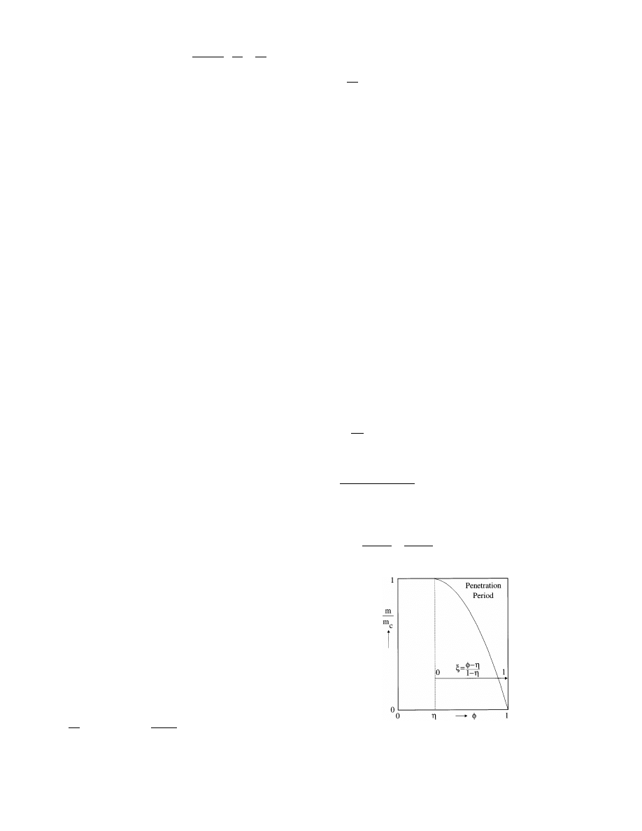
. Similarity of moisture profiles method

This method, developed by Sano and Yamamoto

[21,22], is based on the assumption of similarity of
moisture concentration profiles. A method is given to
also derive diffusion coefficients from the PP drying
curve based on isothermal drying experiments at differ-
ent initial moisture contents. No functional relationship
for the diffusivity has to be put forward. The isother-
mal drying process of an ideally shrinking slab is con-
sidered. The diffusion equation is transformed with the
aid of solid-based parameters (see Table 1) and solved
numerically for several types of diffusivities (e.g. power
law, exponential, linear). The calculated moisture profi-
les are normalized as given below:

versus

f−h

1 −

for the penetration period

(46)

and

versus

j=f for the regular regime

(47)

where m

is the center moisture content and

h indicates

the penetration depth of the moisture profile (see Fig.
9).

The assumption of similarity of moisture profiles

leads to the following two important properties:

(

j) dj=constant

(48)

and

(

f) df=constant

(49)

‘Constant’ means that these parameters do not

change with the average moisture concentration. The
‘constant’ f

(

depends on the material and the initial

moisture content u

, whereas the ‘constant’ f

(

can

only be seen as a material property. Sano and Ya-
mamoto [21,22] arrive, partially via analytical means
and partially by correlating numerical computer output,
at approximate equations for the evaluation of mois-
ture dependent diffusivities from drying curves.

. Penetration period. The following equations

apply:

u = u

(50)

in which

X =

0.807 − 0.470·f

(

1 − 0.99f

(

(51)

From an analytical differentiation the factor

g is

given by

g=1+2

d ln

d ln u

d ln X

d ln u

(52)

Fig. 9. Similarity of moisture concentration profiles during penetra-
tion period.

W.J. Coumans

Chemical Engineering and Processing

39 (2000) 53 – 68

On the basis of the numerical computer output

g can

also be correlated with f

(

according to

0.233 · f

(

(1 − f

(

) · (0.807 − 0.470 · f

(

)

(53)

The factor

b% in Eq. (50) follows directly from the

experimental drying data by

b%= −d

(54)

or by

(1 − m

¯ ) =

1
2

(55)

The evaluation of the moisture dependent diffusion

coefficient from the PP requires several drying curves at
different initial moisture contents u

. Experimental data

values for

b% are obtained from the slope of a plot of m¯

versus

t. From Eqs. (51)–(53) values for g and X are

found via an iterative procedure, which starts with a
zero value for d lnX/d ln(u

). A first estimate of

g is

calculated with Eq. (52), a first approximation of f

(

found from Eq. (53), then X is calculated with Eq. (51).
After having obtained values of X for different values
of u

a better estimate of

g can be made with Eq. (52),

etc. After convergence the obtained values for

g and X

are used to calculate the diffusion coefficient with Eq.
(50).

. Regular regime. The approximate equations are:

= 0.5 · (f

(

)

0.40

u = u

(56)

in which:

u¯

(

¯ · u

(

(57)

and

(

1 +

0.643

−

0.10

with

G =

d ln F

d ln m

(58)

From the RR drying curve F

versus m

¯ and the

above calculation is straightforward.

The method may be used for a non-shrinking slab as

well, under the conditions that a correct transformation
of the parameters is carried out (see Table 1).

. Flux ratio method

The flux ratio method [23,24] is based on the obser-

vation that — at a given average moisture content and a
given boundary moisture content — there is a fairly
constant ratio

a between the non-stationary flux F

and the stationary flux F

. For a slab this ratio

a only

depends on the drying stage.

For the penetration period, the following holds

1 − m

D dm dm

with

= 1.27

(59)

and for the regular regime

D dm

with

= 1.23

(60)

in which the center moisture content m

is related to the

averaged moisture content m

¯ by:

¯ = m

−

D dm dm

D dm

(61)

Deriving diffusion coefficients from the RR drying

curve by this method requires a relationship for D =
D(m) to be put forward. Any analytical function can be
used, however, as a good starting point a power series
of N

order can be tried:

D =

(62)

Power series are more flexible than exponential or

power law functions and are for this reason more
suitable for approximating unknown functions. From
computer simulations it was found that N = 6 satisfies
quite well for several types of relationships D = D(m).

Approximations in case of non-zero boundary condi-

tions are given by Liu and Coumans [12].

. Rigorous numerical methods

In this approach the diffusion equation is solved

numerically for any arbitrary relationship for the mois-
ture concentration dependence of the diffusion coeffi-
cient. For instance the following relationships with two
tunable parameters (a and D

D = D

exp [a(m − 1)]

D = D

(m + a(1 − m))

(63)

The calculated and experimental drying curves F

versus m

¯ are compared and the parameters a and D

are tuned to minimize the sum of squares (SSQ). Be-
cause the drying rates are usually monotonously and
‘relatively slowly’ decreasing as m

¯ decreases, there will

be no problem in obtaining an excellent agreement [25].
Initially this appears good, however, this approach
results in many cases that the SSQ as a function of the
tuning parameters a and D

is rather flat in the neigh-

borhood of the minimum value. This means that in
these cases there exist — within a certain range — many
combinations of the tuning parameters which all lead to
an excellent agreement between calculated and experi-
mental drying curves. So it still remains difficult to
obtain reliable and intrinsic diffusion coefficients.

W.J. Coumans

Chemical Engineering and Processing

39 (2000) 53 – 68

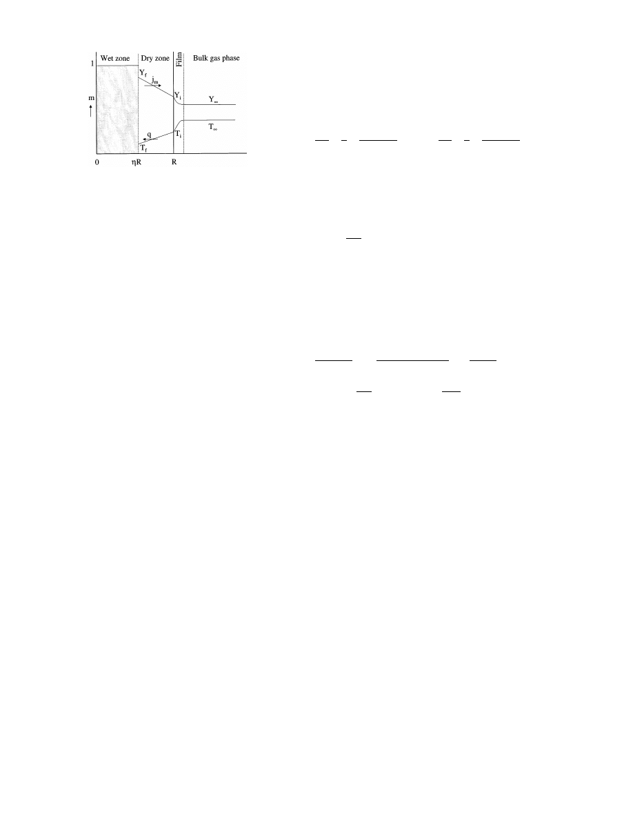
Fig. 10. Uniformly retreating moisture front in a non-hygroscopic
porous material.

In a linearized form the transport fluxes are given by:

= k

eff

− Y

)

and

q =

eff

− T

)

(64)

where the transport coefficients k

eff

and

eff

depend on

the conditions in the gas film and the properties of the
dry zone:

eff

1
k

(1 −

h)R

dry

and

eff

1
a

(1 −

h)R

dry

(65)

The thermal conductivity

dry

of the dry zone has to

be found directly from experiments or via modeling
heat conduction in a two-phase system (parallel model,
series model, etc. [4]). The moisture diffusion coefficient
D

dry

is given by:

dry

(66)

in which D

is the gas diffusion coefficient of vapor in

air, and

m is the so-called diffusion resistance factor [4],

which takes into account the effect of the porous
structure of the dry zone.

Because evaporation takes place at the moisture

front, the ‘wet bulb equation’ for this situation then
reads:

− T

− Y

= −

1 + (1 −

h) · Bi

1 + (1 −

h) · Bi

· L ·

vap

with

dry

and

dry

(67)

As soon as a moisture front is retreating the drying

rate tends to decrease, because the transport resistance
of the dry zone increases. Usually Bi

, which

means that the temperature at the evaporating front
will start to increase, leading to an increase of the
driving force for vapor transport.

. Method of Yoshida et al.

[29

–

31]

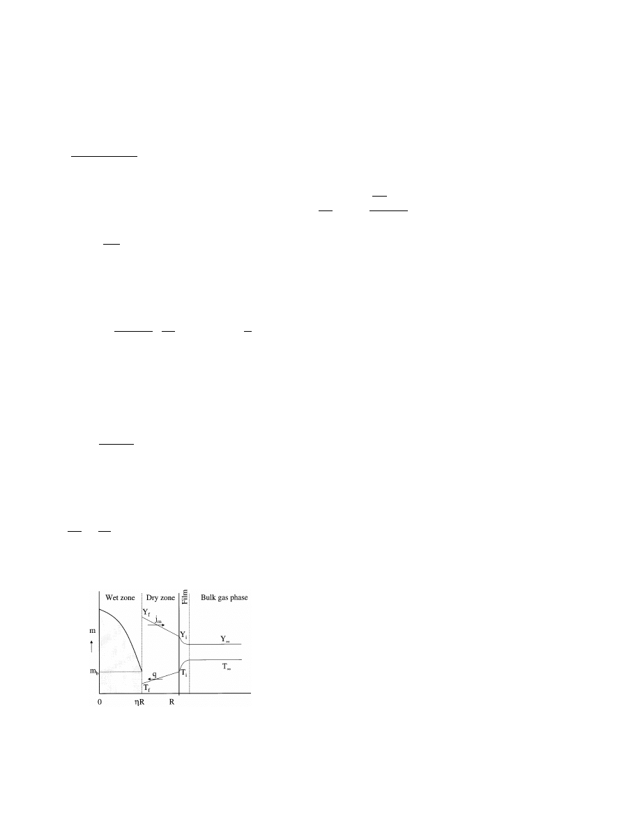
We consider the isothermal drying process of a non-

hygroscopic porous slab at a uniform temperature. At
the beginning all the pores are filled with liquid mois-
ture, so the initial moisture content equals the satura-
tion value. It is assumed that a transitional moisture
content m

exists. At higher moisture contents (m

)

moisture transport takes place by capillary liquid flow
only, whereas at lower moisture contents (m

) the

only transport mechanism is vapor diffusion. During
the CRP, the liquid flow keeps the surface of the slab
sufficiently wet [6]. The FRP starts when the surface
concentration has reached the transitional value m

During the FRP a plane of evaporation in the slab will
move inwards. The slab now consists of an inner wet
zone and an outer dry zone (Fig. 11).

In the wet zone a resistance to the flow of liquid to

the evaporating plane flow is assumed, which can be
expressed by means of a diffusion coefficient D = D(m).
From the foregoing it follows that D = 0 for m

Recently, Van der Zanden [26] developed an iterative

numerical method to obtain the moisture dependent
diffusion coefficient from an experimental drying curve,
given in terms of m

¯ versus t. The advantage of this

method is, that no a priori information about the
relationship D = D(m) is needed. As a first guess some
‘reasonable’ constant value for D is taken. The solution
of the set of equations, obtained from a numerical
discretization scheme for the diffusion equation with
initial and boundary conditions, delivers the moisture
distribution m = m(

f) in the material. A first correction

of this moisture profile is based on the deviation be-
tween the calculated and experimental values for m

¯ .

With this corrected moisture profile as input, the same
set of equations is now used to find ‘better’ values for D
at the grid points. This procedure is repeated until
successive results are within a desired tolerance. Even-
tually, D = D(m) is obtained. The method has been
tested for Kaolin clay and satisfying results have been
obtained.

. Retreating front models

These types of models may apply to porous materi-

als, where during the drying process a retreating mois-
ture front may occur. The capillary liquid flow to the
surface may not be able to sustain the evaporation at
the surface of the material, especially at sufficiently
high drying rates. A dry zone will be formed and the
plane of evaporation will move inwards.

. Uniform retreating moisture front model

(

URMF

)

In the marginal case, where a uniform retreating

moisture front occurs, it is assumed that in the wet zone
the moisture level remains at the saturated level and
that the mechanisms for mass and heat transfer are
taken place in the dry zone only [4,27,28]. Vapor diffu-
sion in the porous structure of the dry zone is the only
internal moisture transport mechanism. Heat transfer is
assumed to take place via conduction in the gas phase
and the solid matrix of the porous material (Fig. 10).

W.J. Coumans

Chemical Engineering and Processing

39 (2000) 53 – 68

The resistance in the dry zone increases as the evapo-

rating plane moves inwards, whereas the driving force
for vapor diffusion (Y

– Y

) remains constant. The

decreasing drying rate is fully controlled by the increas-
ing thickness of the dry zone. The following expression
for the drying rate can be derived from Eqs. (64) and
(65):

1 + (1 −

h)Bi

(68)

in which

h=h(m¯). Via computer simulations with sev-

eral types of D = D(m) also in this case approximate
equations could be derived for the FRP. The PP drying
curve is given by:

1 − m

¯ +

= constant

(69)

and the RR drying curve by the relationship

. =F.(mˆ−m

)

(70)

in which F

. and mˆ are defined as

. =F

h−

¯ +

and

ˆ =

(71)

From experimental drying data F

versus m

¯ the RR

drying curve can be constructed stepwise as follows:

Find F

for the CRP via the theory in Section 2.

Find Bi

from Eq. (68) by using the fact that if

0 also h0.

Thus for this marginal situation holds

lim

) =

1 + Bi

(72)

Find

h=h(m¯) from Eq. (68) by using the experimen-

tal data F

versus m

¯ .

Find m

from the relationship

h=h(m¯) by using the

fact that m

as m

0. Thus:

lim

(

) =

(73)

Now the characteristic curve F

. versus (mˆ−m

) can

be established.

The above procedure looks simple and straightfor-

ward. Unfortunately, the prediction of drying curves at
different conditions is somehow more complicated. Af-
ter having set the new drying conditions in terms of the
initial moisture content, initial drying flux, slab thick-
ness etc., these conditions have to be put into terms of
F

and Bi

. The drying flux F

then follows from Eq.

(68), however the main problem is now to find the
relationship

h=h(m¯). The starting point for solving

this problem is Eq. (71), which is rewritten as:

= − 2 ·

−

¯ +

with

h=1 at m¯=m¯

(74)

in which F

. depends on h and m¯ and is given by the

known RR drying curve. The above equation is an
ordinary differential equation, from which

h=h(m¯)

can be obtained. The boundary condition requires the
critical moisture content m

, which has to be found by

a trial and error procedure. It appears that if m

chosen too high, the calculated drying curve will show
a maximum, whereas if m

is chosen too low the

calculated drying curve will have a discontinuity. Fi-
nally, the constant in the PP drying curve (Eq. (69)) is
found via the intersection of the G-curves, according to
the procedure already given earlier in Section 3.2.4.

Yoshida et al. [31] have extended their method to

non-isothermal conditions as well, however details will
not be given here.

4. Conclusions and perspectives

For isothermal drying slabs of porous and non-

porous materials an overview is given of (approximate)
methods for the characterization and description of the
drying kinetics. For the time being it is not yet possible
to judge the practical usefulness and reliability of these
methods. Most of them have been developed via com-
puter simulations. However, real and thorough experi-
mental validations are scarce. Kerkhof [32] studied
several drying kinetics models in the simulation of a
fluidized-bed drying process of bio-products and ob-
served unacceptable deviations with respect to the ‘ex-
act’ behavior. It is suggested that most approximate
models are not able to deal in a correct way with
non-zero and time-dependent boundary conditions. In
general, there is a need for more experimental valida-
tion and for establishing the usefulness of the approxi-
mate methods in overall models for industrial drying
processes. This should be done for many different
materials, in order to find criteria to decide which
approximate method should be preferred in a given
situation and to stimulate further developments.

Fig. 11. Retreating moisture front in a non-hygroscopic porous
material with a transitional moisture content m

and a resistance to

liquid flow in the wet zone.

W.J. Coumans

Chemical Engineering and Processing

39 (2000) 53 – 68

As explained extensively in this paper, slab drying

experiments (

3 mm thickness) are used to find the

drying characteristic of a certain material. In the case of
carbohydrate solutions, for example, this information
might be used to describe the drying behavior of
droplets (

0.1 mm diameter) in a spray dryer, or in

case of concentrated clay slurries to describe the drying
behavior of a clay form (

100 mm size) in a drying

chamber. Not much information is available about the
accuracy of the obtained drying kinetics in case of
up-scaling, down-scaling and different geometries of the
drying body. Nor do we know how well or how bad
these models will work in real drying practice, both for
design, control and optimization purposes.

Usually drying curves are monotonously decreasing

functions with time. In case an excellent agreement
between experiment and model is obtained, it does not
really say anything about the correctness of the model.
It is not too difficult to describe a monotonously de-
creasing function, because many two parameter func-
tions may do the work sufficiently well. It is
recommended that for approximate methods, that re-
quire a priori information about the type of diffusion
relationship D = D(m), more physical information
should be inserted. This conclusion is also underlined
by Ketelaars et al. [33], who have shown the discrepan-
cies between the diffusivities obtained from moisture
profiles and drying curves.

In order to arrive at better and validated approxi-

mate methods for the drying kinetics, there are nowa-
days three powerful tools available. Firstly, the
continuously increasing speed of computers, enabling
readily simulations on the basis of sophisticated and
physically based models [34,35]. Secondly, NMR-imag-
ing techniques, allowing a detailed scanning of transient
moisture concentration profiles during drying [35 – 37].
Scanning of moisture profiles during a drying process
delivers a huge amount of data enabling the direct
calculation of the moisture dependent diffusivity. More-
over, this technique also enables the assumptions being
made in the models, e.g. the occurrence of a retreating
moisture front, the speed of this front, and may reveal
surprising information. For instance, usually one ex-
pects a retreating moisture front to move linearly with
the square root of time, surprisingly it was found by Pel
[36] that in bricks this front moves linearly with time!
Thirdly, present laboratory equipment, stuffed with all
types of handy software, enables increasingly more
accurate and reliable experiments. One should not un-
derestimate the experimental problems to carry out slab
drying experiments under well-defined conditions. Some
presented methods require higher order derivatives of
the experimental data. Smoothing and regression tech-
niques are often necessary to obtain stable results. One
should strive for the lowest possible noise of the raw
data and thus one should put the highest possible

demands on the accuracy and stability of the experi-
mental techniques, especially in case of strongly mois-
ture dependent diffusion behavior.

5. Nomenclature

parameter in diffusion relationships

D = D(m)

thermodynamic activity

surface area (m

)

Biot number (Table 1)

Biot number for heat transfer

Biot number for mass transfer

specific heat (J/kg

intrinsic solids density (kg solid/m

solid)

diffusion coefficient (m

/s)

diffusion coefficient at initial moisture

concentration (m

/s)

reduced diffusion coefficient (Table 1)

activation energy of RR drying rate (J/
mol)

normalised drying rate in CDC
reduced moisture concentration in PP

(Eq. (46))
reduced moisture concentration in RR

(Eq. (47))
dimensionless flux parameter (Table 2)

F
F

reduced flux parameter (Table 2)
reduced flux parameter (Table 2)

reduced flux parameter (Eq. (71))

help function (Eq. (40))

G
DH

vap

enthalpy of evaporation (J/kg)
moisture flux (kg/m

mass transfer coefficient (m/s)
permeability (m

)

K
Le

Lewis number
moisture concentration (Table 1)

m
m

averaged moisture concentration
moisture concentration (Eq. (14))

m’

moisture concentration (Eq. (71))

transitional bound moisture

concentration
molecular weight of drying gas (kg/

mol)
mass of solids (kg)

molecular weight of vapour (kg/mol)
constant (Eq. (29))

p
P

total pressure (N/m

)

vapour pressure (N/m

)

saturation vapour pressure (N/m

)

v, sat

constant (Eq. (28))

heat flux (J/m

q
r

space co-ordinate (m)

half thickness of two sided drying slab
(m)

W.J. Coumans

Chemical Engineering and Processing

39 (2000) 53 – 68

gas constant (J/mol K)

solids radius (m)
relative humidity

time (s)

temperature (

T
u

moisture concentration (kg moisture/kg

dry solid)

moisture concentration at interface (kg

moisture/kg dry solid)

moisture concentration in centre (kg

moisture/kg dry solid)

averaged moisture concentration (kg

u¯

moisture/kg dry solid)

velocity (m/s)

volume (m

)

help function (Eq. (50))

air humidity (kg moisture/kg dry air)

Greek

heat transfer coefficient (W/m

2 o

constant in flux ratio method (Eq.

(59))

constant in flux ratio method (Eq.

(60))

measure for drying rate (Eqs. (54) and

b’

(55))

space co-ordinate (Table 1)

normalised moisture concentration
help function (Eq. (50))

relative penetration depth (Fig. 9)

relative position of moisture front (Fig.

10)

psychrometric ratio

viscosity (kg/ms)
moisture concentration (kg/m

)

solids concentration (kg/m

)

density of humid air (kg/m

)

time (Table 1)

normalised space co-ordinate during

PP (Eq. (46))

Subscripts
‘overline’

space averaged value
air

bound

centre

critical

constant rate period

CRP

effective

eff

equilibrium

eq
f

front
gas

heat

interface

moisture

mass

Penetration period

Regular regime

RR
s

solid
saturated

sat

total

t
T

transition from PP to RR
vapour

vapour/air

vaporisation

vap

wet bulb conditions

wet

initial, at t = 0

bulk of drying gas

Abbre

6iations

boundary condition
characteristic drying curve

CDC

constant rate period

CRP
FRP

falling period
initial condition

penetration period

regular regime

uniformly retreating moisture front

URMF

References

[1] J. Crank, The mathematics of diffusion, 2nd edition, Oxford

University Press, 1990.

[2] J.S. Vrentas, J.L. Duda, Molecular diffusion in polymer solu-

tions, A.I.Ch.E.J. 25 (1) (1979) 1 – 24.

[3] S. Whitaker, Simultaneous heat, mass, and momentum transfer

in porous media: a theory of drying, Adv. Heat Mass Transf.
13 (1977) 110 – 203.

[4] O. Krischer, W. Kast, Trocknungstechnik, Band 1, Die wis-

senschaftlichen Grundlagen der Trocknungstechnik, Springer-
Verlag, 1978.

[5] R.B. Keey, Drying; Principles and Practice, Pergamon Press,

Oxford, 1972.

[6] E.U. Schlu¨nder, On the mechanism of the constant drying rate

period and its relevance to diffusion controlled catalytic gas
phase reactions, Chem. Eng. Sci. 43 (10) (1988) 2685 – 2688.

[7] D.A. Van Meel, Adiabatic convection batch drying with recir-

culation of air, Chem. Eng. Sci. 9 (1958) 36 – 44.

[8] R.B. Keey, M. Suzuki, On the characteristic drying curve, Int.

J. Heat Mass Trans. 17 (12) (1974) 1455 – 1464.

[9] Q.J. Zhang, R.B. Keey, T.A.G. Langrish, H.S. Pasley, I.C.

Kemp, An experimental test of the concept of the characteris-
tic drying curve using the thin-layer method, in: V. Rudolph,
R.B. Keey, A.S. Mujumdar (Eds.), Drying 94 (Proceedings of
the 9th International Drying Symposium), vol. A, 1994, pp.
123 – 131.

[10] E.U. Schlu¨nder, Fortschritte und Entwicklungstendenzen bei

der

Auslegung

von

Trocknern

fu¨r

Vorgeformte

Trock-

nungsgu¨ter, Chem. Ing. Techn. 48 (3) (1976) 190 – 198.

[11] S. Yamamoto, M. Hoshika, Y. Sano, Determination of con-

centration dependent diffusion coefficient from drying rates, in:
Proceedings of 4th International Drying Symposium, Kyoto,
Japan, Hemisphere, NY, 1984.

W.J. Coumans

Chemical Engineering and Processing

39 (2000) 53 – 68

[12] T. Liu, W.J. Coumans, Approximate solutions of diffusion equa-

tion with non-zero and time dependent boundary concentration,
in: Proc. 10th International Drying Symposium, Krakow,
Poland, vol. A, 1996, pp. 167 – 174.

[13] J.K. Liou, S. Bruin, An approximate method for the nonlinear

diffusion problem with a power relation between diffusion coeffi-
cient and concentration (Part I and Part II), Int. J. Mass Heat
Transf. 25 (1982) 1209 – 1229.

[14] Coumans, W.J., 1987. Power law diffusion in drying processes.

Ph.D. thesis, Eindhoven University of Technology.

[15] W.J. Coumans, K.Ch.A.M. Luyben, Evaluation and prediction

of experimental drying curves of slabs, in: S. Bruin (Ed.), Pro-
ceedings of the International Symposium on Preconcentration
and Drying of Foods (Thijssen Memorial Symposium), Elsevier,
1988, pp. 163 – 172.

[16] S. Yamamoto, W.J. Coumans, T. Vlugt, Determining concentra-

tion dependent diffusivity in food materials, in: R. Jowitt (Ed.),
Proceedings of the 7th International Congress on Engineering
and Food (ICEF7), Brighton, Part 1, 1997, pp. A164 – 167.

[17] Schoeber, W.J.A.H., 1976. Regular Regimes in Sorption Pro-

cesses. Ph.D. Thesis, Eindhoven.

[18] W.J.A.H. Schoeber, A short cut method for the calculation of

drying rates in case of a concentration dependent diffusion
coefficient, in: Proceedings of the First International Drying
Symposium, 1978, pp. 1 – 9.

[19] K.C.A.M. Luyben, J.J. Olieman, S. Bruin, Concentration depen-

dent diffusion coefficients derived from experimental drying
curves, in: A.S. Mujumdar (Ed.), Drying 1980 (Proceedings of
the 2nd International Drying Symposium), vol. 2, Hemisphere
Publishing, 1980, pp. 233 – 243.

[20] T. Liu, W.J. Coumans, Regular regime analysis and moisture

diffusivity in wood, Drying Technol. 11 (5) (1993) 977 – 1003.

[21] Y. Sano, S. Yamamoto, Diffusion coefficient based on the

assumption of similar concentration distribution, in: Drying
1986 (Proceedings of the 5th International Drying Symposium),
vol. 1, 1986, pp. 85 – 93.

[22] Y. Sano, S. Yamamoto, Calculation of concentration dependent

mutual diffusion coefficient in desorption of film, J. Chem. Eng.
Japan 23 (No.3) (1990) 331 – 338.

[23] M. Yoshida, H. Imakoma, M. Okazaki, Determination of diffu-

sivity using the characteristic function for the regular regime, J.
Chem. Eng. Japan 24 (6) (1991) 720 – 726.

[24] M. Legros, H. Imakoma, M. Yoshida, M. Okazaki, Approxi-

mate isothermal drying curves of hygroscopic porous materials
with given desorption isotherm, Chem. Eng. Process. 31 (1992a)
149 – 155.

[25] Ketelaars, A.A.J., 1992. Drying Deformable Media. Ph.D. The-

sis, Eindhoven.

[26] A.J.J. Van der Zanden, An iterative procedure to obtain the

concentration dependency of the diffusion coefficient from the
space averaged concentration versus time, Chem. Eng. Sci. 53
(No.7) (1998) 1397 – 1404.

[27] Haertling, M., 1978. Messung und Analyse von Trocknungsver-

laufskurven als Grundlage zur Vorausberechnung von Trock-
nungsprozessen. Dissertation, Karlsruhe.

[28] M. Haertling, Vorausberechnung von Trocknungsverlaufskur-

ven, VT-Verfahrenstechnik, Band 13, vol. 12, 1979, pp. 923 – 927.

[29] M. Yoshida, H. Imakoma, M. Okazaki, Characteristic functions

for the drying of non-hygroscopic porous slab with a constant
body temperature, J. Chem. Eng. Japan 23 (1990) 58 – 63.

[30] M. Yoshida, H. Imakoma, M. Okazaki, Estimation of isother-

mal drying rates for non-hygroscopic porous slabs using charac-
teristic functions, J. Chem. Eng. Japan 23 (1990) 502 – 505.

[31] M. Yoshida, H. Imakoma, M. Okazaki, Estimation of drying

rate curves for non-hygroscopic porous slabs using the character-
istic function for the regular regime, Chem. Eng. Process. 30
(1991) 87 – 96.

[32] P.J.A.M. Kerkhof, A test of lumped parameter methods for the

drying rate in fluidized bed dryers for bio-products, in: Drying
1994 (Proceedings of the 9th International Drying Symposium),
vol. A, 1994, pp. 132 – 140.

[33] T. Ketelaars, L. Pel, W.J. Coumans, P.J.A.M. Kerkhof, Drying

kinetics; a comparison of diffusion coefficients from moisture
concentration profiles and drying curves, Chem. Eng. Sci. 50 (7)
(1995) 1187 – 1191.

[34] Couture, F., 1995. Mode´lisation fine d’un proble`me de se´chage,

de´veloppement d’outils adapte´s. Ph.D. Thesis, University of
Bordeaux.

[35] Kroes, B., 1999. The influence of material properties on drying

kinetics. Ph.D. Thesis, Eindhoven.

[36] Pel, L., 1995. Moisture transport in porous building materials.

Ph.D. Thesis, Eindhoven.

[37] B. Kroes, W.J. Coumans, L. Pel, P.J.A.M. Kerkhof, Validation

of a physically based drying model with the aid of NMR-imag-
ing, in: Drying 1998, vol. A, 1998, pp. 264 – 271.

Wyszukiwarka

Podobne podstrony:
PWR A Full Compensating System for General Loads, Based on a Combination of Thyristor Binary Compens
Adjustable Speed Generators For Wind Turbines Based On Doubly
Comparative study based on exergy analysis of solar air heater collector using thermal energy storag
Drying kinetics and drying shrinkage of garlic subjected to vacuum microwave dehydration (Figiel)
ITU T standardization activities for interactive multimedia communications on packet based networks
Drying kinetics and drying shrinkage of garlic subjected to vacuum microwave dehydration (Figiel)
Microwave drying characteristics of potato and the effect of different microwave powers on the dried
Queuing theory based models for studying intrusion evolution and elimination in computer networks
Box Wagon box for drying hay
Effect of drying conditions on the quality of vacuum microwave dried potato cubes
Daniel H Cheever A New Methodology for Audio Frequency Power Amplifier Testing Based On Psychoacoust
Novel Multi level Inverter Topology Based on Multi Winding Multi Trapped Transformers for Improved W
053 Cost Estimation Methods for Drying
Electrochemical DNA biosensors based on platinum nanoparticles combined carbon nanotubes
PCB layout tuner layout for H LCD2005 from KTV on 5Jun
36 495 507 Unit Cell Models for Thermomechanical Behaviour of Tool Steels

więcej podobnych podstron