( SPC ) STASTICAL PROCESS CONTROL REFERENCE MANUAL

Issued 1992, Second Printing March 1995 (new cover only)

Chrysler Corporation, Ford Motor Company, and General Motors Corporation

REFERENCE MANUAL

STATISTICAL PROCESS

CONTROL

(SPC)

FOREWORD

This Reference Manual was prepared by the quality and supplier assessment staffs at Chrysler, Ford
and General Motors, working under the auspices of the Automotive Division of the American Society
for Quality Control Supplier Quality Requirements Task Force, in collaboration with the Automotive
Industry Action Group.

The ASQC/AIAG Task Force charter is to standardize the reference manuals, reporting formats and
technical nomenclature used by Chrysler, Ford and General Motors in their respective supplier
assessment systems: Supplier Quality Assurance, Total Quality Excellence and Targets for Excellence.
Accordingly, this Reference Manual can be used by any supplier to develop information responding to
the requirements of either Chrysler’s, Ford’s or General Motors’ supplier assessment systems.

Until now, there has been no unified formal approach in the automotive industry on statistical process
control. Certain manufacturers provided methods for their suppliers, while others had no specific
requirements. In an effort to simplify and minimize variation in supplier quality requirements, Chrysler,
Ford, and General Motors agreed to develop and, through AIAG, distribute this manual. The work
team responsible for the Manual’s content was led by Leonard A. Brown of General Motors.

The manual should be considered an introduction to statistical process control. It is not intended to
limit evolution of statistical methods suited to particular processes or commodities nor is it intended
to be comprehensive of all SPC techniques. Questions on the use of alternate methods should be
referred to your customer’s quality activity.

The Task Force gratefully acknowledges: the senior leadership and commitment of Vice Presidents
Thomas T. Stallkamp at Chrysler, Clinton D. Lauer at Ford, and Donald A. Pais at General Motors;
the technical competence and hard work of their quality and supplier assessment teams; and the
invaluable contributions of the Automotive Industry Action Group (under AIAG Executive Director
Joseph R. Phelan) in the development, production and distribution of this Reference manual.

We also wish to thank the ASQC reading team led by Tripp Martin of Peterson Spring, who reviewed
the Manual and in the process made valuable contributions to intent and content.

Bruce W. Pince
Task Force Coordinator
Sandy Corporation
Troy, Michigan
December, 1991

This Manual is copyrighted by

Chrysler Corporation, Ford Motor Company, General Motors Corporation

all rights reserved, 1991. Additional copies can be ordered from A.I.A.G., and/or permission to copy
portions of the Manual for use within supplier organizations may be obtained from A.I.A.G. at (248)
358-3570.

ACKNOWLEDGEMENT

The joint consensus on the contents of this document was effected through Task Team Subcommittee
Members representing General Motors, Ford, and Chrysler, respectively, whose approval signatures
appear below, and who gratefully acknowledge the significant contribution of Pete Jessup of the Ford
Motor Company, who was responsible for developing the majority of the material found in Chapters I,
II, and III, and the Appendix of this document.

Harvey Goltzer of the Chrysler Corporation contributed concepts relative to process capability and
capability studies, found in the introduction section of Chapter I. Jack Herman of Du Pont contrib-
uted some of the concepts relative to capability and performance indices and the importance of mea-
surement variability, found in portions of Chapters II and IV, respectively.

The General Motors Powertrain Division contributed the discussion and examples relative to
subgrouping and process overadjustment. The section in Chapter II which provides understanding of
process capability and related issues was developed by the General Motors Corporate Statistical Re-
view Committee. This committee also contributed to the development of Chapter IV, Process Mea-
surement Systems Analysis, as well as to some Appendix items.

Finally, valuable input to all sections of the manual was provided by ASQC representatives Greg
Gruska, Doug Berg, and Tripp Martin.

Leonard A. Brown, G.M.

Victor W. Lowe, Jr., Ford

David R. Benham, Chrysler

December 1991

TABLE OF CONTENTS

Chapter I

INTRODUCTION TO CONTINUAL IMPROVEMENT AND

STATISTICAL PROCESS CONTROL . . . . . . . . . . . . . . . . . . . . . . . . . . . . . . . . . . . . 1

Section 1 PREVENTION VERSUS DETECTION . . . . . . . . . . . . . . . . . . . . . . . . . 5

Section 2 A PROCESS CONTROL SYSTEM . . . . . . . . . . . . . . . . . . . . . . . . . . . . . 7

Section 3 VARIATION: COMMON AND SPECIAL CAUSES . . . . . . . . . . . . . . . . 9

Section 4 LOCAL ACTIONS AND ACTIONS ON THE SYSTEM . . . . . . . . . . . . 11

Section 5 PROCESS CONTROL AND PROCESS CAPABILITY . . . . . . . . . . . . 13

Section 6 THE PROCESS IMPROVEMENT CYCLE AND

PROCESS CONTROL . . . . . . . . . . . . . . . . . . . . . . . . . . . . . . . . . . . . . . 17

Section 7 CONTROL CHARTS: TOOLS FOR PROCESS CONTROL . . . . . . . . 21

Section 8 BENEFITS OF CONTROL CHARTS . . . . . . . . . . . . . . . . . . . . . . . . . . 25

Chapter II

CONTROL CHART FOR VARIABLES . . . . . . . . . . . . . . . . . . . . . . . . . . . . . . . . . . 27

Section 1 AVERAGE AND RANGE CHARTS ( X AND R ) . . . . . . . . . . . . . . . . . 29

A. GATHER DATA . . . . . . . . . . . . . . . . . . . . . . . . . . . . . . . . . . . . . . . . . . . . 31

B. CALCULATE CONTROL LIMITS . . . . . . . . . . . . . . . . . . . . . . . . . . . . . 37

C. INTERPRET FOR PROCESS CONTROL . . . . . . . . . . . . . . . . . . . . . . . 39

D. INTERPRET FOR PROCESS CAPABILITY . . . . . . . . . . . . . . . . . . . . . 57

Section 2 AVERAGE AND STANDARD DEVIATION CHARTS

( X AND s) . . . . . . . . . . . . . . . . . . . . . . . . . . . . . . . . . . . . . . . . . . . . . . . . . 65

A. GATHER DATA . . . . . . . . . . . . . . . . . . . . . . . . . . . . . . . . . . . . . . . . . . . . 65

B. CALCULATE CONTROL LIMITS . . . . . . . . . . . . . . . . . . . . . . . . . . . . . 67

C. INTERPRET FOR PROCESS CONTROL . . . . . . . . . . . . . . . . . . . . . . . 67

D. INTERPRET FOR PROCESS CAPABILITY . . . . . . . . . . . . . . . . . . . . . 67

Section 3 MEDIAN CHARTS ( X AND R) . . . . . . . . . . . . . . . . . . . . . . . . . . . . . . . 69

A. GATHER DATA . . . . . . . . . . . . . . . . . . . . . . . . . . . . . . . . . . . . . . . . . . . . 69

B. CALCULATE CONTROL LIMITS . . . . . . . . . . . . . . . . . . . . . . . . . . . . . 69

C. INTERPRET FOR PROCESS CONTROL . . . . . . . . . . . . . . . . . . . . . . . 71

D. INTERPRET FOR PROCESS CAPABILITY . . . . . . . . . . . . . . . . . . . . . 71

E. ALTERNATE APPROACH TO MEDIAN CHART . . . . . . . . . . . . . . . . . 72

Section 4 CHARTS FOR INDIVIDUALS AND MOVING RANGE (X–MR) . . . . 75

A. GATHER DATA . . . . . . . . . . . . . . . . . . . . . . . . . . . . . . . . . . . . . . . . . . . . 75

B. CALCULATE CONTROL LIMITS . . . . . . . . . . . . . . . . . . . . . . . . . . . . . 75

C. INTERPRET FOR PROCESS CONTROL . . . . . . . . . . . . . . . . . . . . . . . 77

D. INTERPRET FOR PROCESS CAPABILITY . . . . . . . . . . . . . . . . . . . . . 77

Section 5 UNDERSTANDING PROCESS CAPABILITY AND PROCESS

PERFORMANCE FOR VARIABLES DATA . . . . . . . . . . . . . . . . . . . . . 79

A. DEFINITIONS OF PROCESS TERMS . . . . . . . . . . . . . . . . . . . . . . . . . . 79

B. DEFINITION OF PROCESS MEASURES . . . . . . . . . . . . . . . . . . . . . . . 80

C. DESCRIPTION OF CONDITIONS AND ASSUMPTIONS . . . . . . . . . . 81

D. SUGGESTED USE OF PROCESS MEASURES . . . . . . . . . . . . . . . . . . 83

TABLE OF CONTENTS – Continued

Chapter III CONTROL CHARTS FOR ATTRIBUTES . . . . . . . . . . . . . . . . . . . . . . . . . . . . . . . . 89

Section I THE p CHART FOR PROPORTION NONCONFORMING . . . . . . . . 91

A. GATHER DATA . . . . . . . . . . . . . . . . . . . . . . . . . . . . . . . . . . . . . . . . . . . . 93

B. CALCULATE CONTROL LIMITS . . . . . . . . . . . . . . . . . . . . . . . . . . . . . 95

C. INTERPRET THE CHART FOR PROCESS CONTROL . . . . . . . . . . . . 99

D. INTERPRET FOR PROCESS CAPABILITY . . . . . . . . . . . . . . . . . . . . 107

Section 2 THE np CHART FOR NUMBER NONCONFORMING . . . . . . . . . . . 111

A. GATHER DATA . . . . . . . . . . . . . . . . . . . . . . . . . . . . . . . . . . . . . . . . . . . 111

B. CALCULATE CONTROL LIMITS . . . . . . . . . . . . . . . . . . . . . . . . . . . . 111

C. INTERPRET FOR PROCESS CONTROL . . . . . . . . . . . . . . . . . . . . . . 111

D. INTERPRET FOR PROCESS CAPABILITY . . . . . . . . . . . . . . . . . . . . 111

Section 3 THE c CHART FOR NUMBER OF NONCONFORMITIES . . . . . . . . 113

A. GATHER DATA . . . . . . . . . . . . . . . . . . . . . . . . . . . . . . . . . . . . . . . . . . . 113

B. CALCULATE CONTROL LIMITS . . . . . . . . . . . . . . . . . . . . . . . . . . . . 113

C. INTERPRET FOR PROCESS CONTROL . . . . . . . . . . . . . . . . . . . . . . 113

D. INTERPRET FOR PROCESS CAPABILITY . . . . . . . . . . . . . . . . . . . . 113

Section 4 THE u CHART FOR NONCONFORMITIES PER UNIT . . . . . . . . . . 115

A. GATHER DATA . . . . . . . . . . . . . . . . . . . . . . . . . . . . . . . . . . . . . . . . . . . 115

B. CALCULATE CONTROL LIMITS . . . . . . . . . . . . . . . . . . . . . . . . . . . . 115

C. INTERPRET FOR PROCESS CONTROL . . . . . . . . . . . . . . . . . . . . . . 117

D. INTERPRET FOR PROCESS CAPABILITY . . . . . . . . . . . . . . . . . . . . 117

Chapter IV PROCESS MEASUREMENT SYSTEMS ANALYSIS . . . . . . . . . . . . . . . . . . . . . . . 119

Section 1 INTRODUCTION . . . . . . . . . . . . . . . . . . . . . . . . . . . . . . . . . . . . . . . . . . 119

Section 2 AVERAGE AND RANGE METHOD . . . . . . . . . . . . . . . . . . . . . . . . . . 121

A. CONDUCTING THE STUDY . . . . . . . . . . . . . . . . . . . . . . . . . . . . . . . . 121

B. CALCULATIONS . . . . . . . . . . . . . . . . . . . . . . . . . . . . . . . . . . . . . . . . . 122

C. ANALYSIS OF RESULTS . . . . . . . . . . . . . . . . . . . . . . . . . . . . . . . . . . . 123

D. EXAMPLE . . . . . . . . . . . . . . . . . . . . . . . . . . . . . . . . . . . . . . . . . . . . . . . 127

APPENDICES

SOME COMMENTS ON SUBGROUPING . . . . . . . . . . . . . . . . . . . . . . . . . . . . . . . . . . . 131

OVERADJUSTMENT . . . . . . . . . . . . . . . . . . . . . . . . . . . . . . . . . . . . . . . . . . . . . . . . . . . . 137

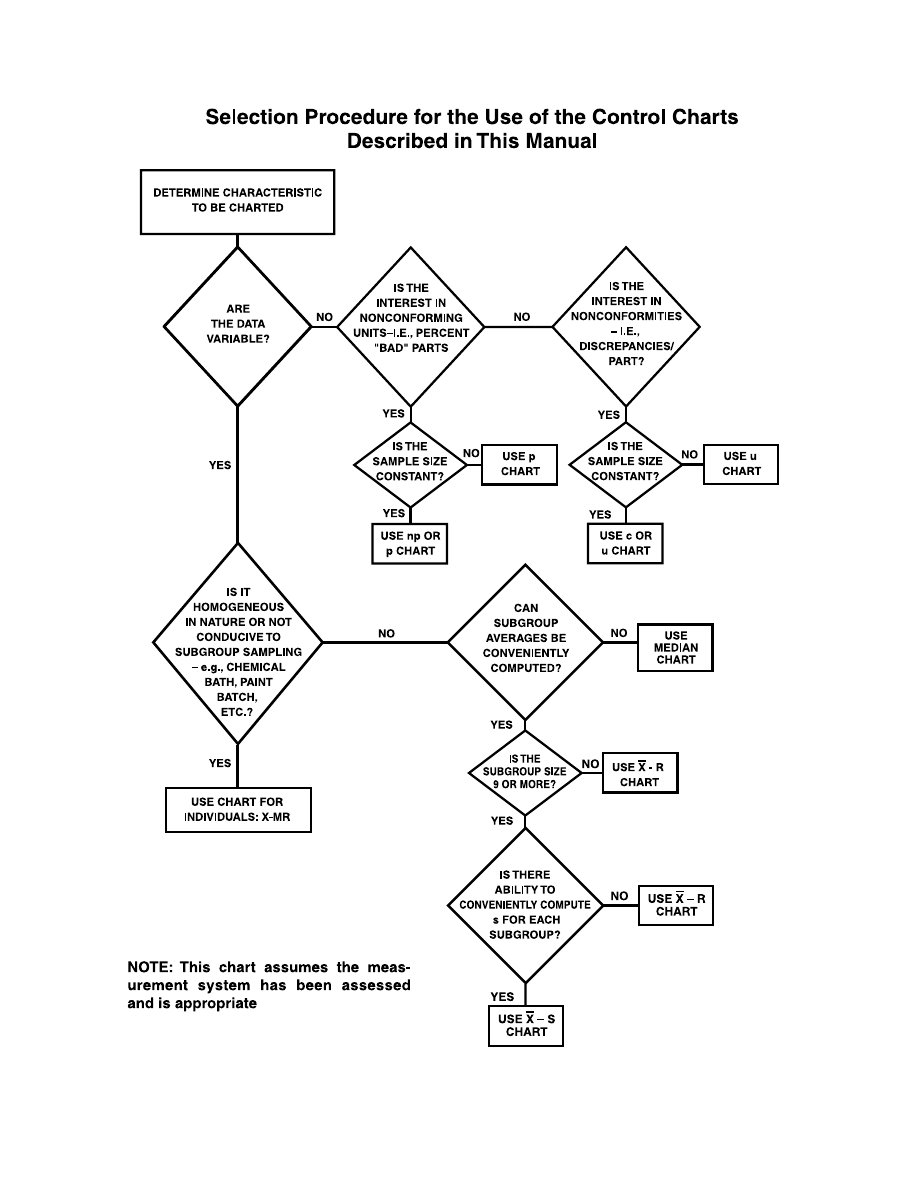
SELECTION PROCEDURE FOR THE USE OF THE CONTROL CHARTS
DESCRIBED IN THIS MANUAL . . . . . . . . . . . . . . . . . . . . . . . . . . . . . . . . . . . . . . . . . . . 139

RELATIONSHIP BETWEEN Cpm AND OTHER INDICES WITH
(USL – T) = (T – LSL) . . . . . . . . . . . . . . . . . . . . . . . . . . . . . . . . . . . . . . . . . . . . . . . . . . . . . 141

TABLE OF CONSTANTS AND FORMULAS FOR CONTROL CHARTS . . . . . . . . . . 143

STANDARD NORMAL DISTRIBUTION . . . . . . . . . . . . . . . . . . . . . . . . . . . . . . . . . . . . 147

GLOSSARY OF TERMS AND SYMBOLS . . . . . . . . . . . . . . . . . . . . . . . . . . . . . . . . . . . . 149

REFERENCES AND SUGGESTED READINGS . . . . . . . . . . . . . . . . . . . . . . . . . . . . . 159

REPRODUCIBLE COPIES OF CONTROL CHART FORMS . . . . . . . . . . . . . . . . . . . 161

LIST OF ILLUSTRATIONS

Figure

Title

Page

A Process Control System . . . . . . . . . . . . . . . . . . . . . . . . . . . . . . . . . . . . . . . . . . . . . . 6

Variation: Common and Special Causes . . . . . . . . . . . . . . . . . . . . . . . . . . . . . . . . . . . 8

Process Control and Process Capability . . . . . . . . . . . . . . . . . . . . . . . . . . . . . . . . . . . 12

The Process Improvement Cycle . . . . . . . . . . . . . . . . . . . . . . . . . . . . . . . . . . . . . . . . . 16

Control Charts . . . . . . . . . . . . . . . . . . . . . . . . . . . . . . . . . . . . . . . . . . . . . . . . . . . . . . . 20

Variables Data – Results from Measuring Intermediate or
Final Process Outcome . . . . . . . . . . . . . . . . . . . . . . . . . . . . . . . . . . . . . . . . . . . . . . . . 26

X and R Chart . . . . . . . . . . . . . . . . . . . . . . . . . . . . . . . . . . . . . . . . . . . . . . . . . . . . . . . 30

X and R Chart – Setup Data . . . . . . . . . . . . . . . . . . . . . . . . . . . . . . . . . . . . . . . . . . . . 32

X and R Chart – “Initial Study” . . . . . . . . . . . . . . . . . . . . . . . . . . . . . . . . . . . . . . . . . . 34

X and R Chart – With Control Limits . . . . . . . . . . . . . . . . . . . . . . . . . . . . . . . . . . . . . 36

R Chart – Point Beyond Control Limits . . . . . . . . . . . . . . . . . . . . . . . . . . . . . . . . . . . 38

R Chart – Runs (Range) . . . . . . . . . . . . . . . . . . . . . . . . . . . . . . . . . . . . . . . . . . . . . . . . 40

R Chart – Nonrandom Patterns . . . . . . . . . . . . . . . . . . . . . . . . . . . . . . . . . . . . . . . . . 42

X and R Chart – Control Limits Recalculation (Range) . . . . . . . . . . . . . . . . . . . . . . . 44

X Chart – Points Beyond Control Limits . . . . . . . . . . . . . . . . . . . . . . . . . . . . . . . . . . . 46

X Chart – Runs . . . . . . . . . . . . . . . . . . . . . . . . . . . . . . . . . . . . . . . . . . . . . . . . . . . . . . 48

X Chart – Nonrandom Patterns . . . . . . . . . . . . . . . . . . . . . . . . . . . . . . . . . . . . . . . . . 50

X and R Chart – Control Limits Recalculation . . . . . . . . . . . . . . . . . . . . . . . . . . . . . . 52

X and R Chart – Extended Limits . . . . . . . . . . . . . . . . . . . . . . . . . . . . . . . . . . . . . . . . 54

Process Variation Relative To Specification Limits . . . . . . . . . . . . . . . . . . . . . . . . . . . 56

Calculating the Process Capability . . . . . . . . . . . . . . . . . . . . . . . . . . . . . . . . . . . . . . . 58

Evaluating the Process Capability . . . . . . . . . . . . . . . . . . . . . . . . . . . . . . . . . . . . . . . 60

Data Collection . . . . . . . . . . . . . . . . . . . . . . . . . . . . . . . . . . . . . . . . . . . . . . . . . . . . . . 64

X and s Chart . . . . . . . . . . . . . . . . . . . . . . . . . . . . . . . . . . . . . . . . . . . . . . . . . . . . . . . . 66

Median Control Chart . . . . . . . . . . . . . . . . . . . . . . . . . . . . . . . . . . . . . . . . . . . . . . . . . 68

Median Control Chart – Interpretation . . . . . . . . . . . . . . . . . . . . . . . . . . . . . . . . . . . . 70

Individuals and Moving Range Chart . . . . . . . . . . . . . . . . . . . . . . . . . . . . . . . . . . . . . 74

Interpretation of Individuals and Moving Range Chart . . . . . . . . . . . . . . . . . . . . . . . 76

“Goal Post” vs. Loss Function . . . . . . . . . . . . . . . . . . . . . . . . . . . . . . . . . . . . . . . . . . . 82

Process Alignment to Requirements . . . . . . . . . . . . . . . . . . . . . . . . . . . . . . . . . . . . . . 84

Attribute Data . . . . . . . . . . . . . . . . . . . . . . . . . . . . . . . . . . . . . . . . . . . . . . . . . . . . . . . 88

p Chart for Proportion Nonconforming – Gathering Data . . . . . . . . . . . . . . . . . . . . . 92

p Chart for Proportion Nonconforming – Calculating
Control Limits, Sheet 1 . . . . . . . . . . . . . . . . . . . . . . . . . . . . . . . . . . . . . . . . . . . . . . . . 94

p Chart for Proportion Nonconforming – Calculating
Control Limits, Sheet 2 . . . . . . . . . . . . . . . . . . . . . . . . . . . . . . . . . . . . . . . . . . . . . . . . 96

p Chart for Proportion Nonconforming – Points Beyond
Control Limits . . . . . . . . . . . . . . . . . . . . . . . . . . . . . . . . . . . . . . . . . . . . . . . . . . . . . . . 98

p Chart for Proportion Nonconforming – Runs . . . . . . . . . . . . . . . . . . . . . . . . . . . . . 100

p Chart for Proportion Nonconforming – Nonrandom Patterns . . . . . . . . . . . . . . . . 102

LIST OF ILLUSTRATIONS – Continued

Figure

Title

Page

p Chart for Proportion Nonconforming – Control Limits Recalculation . . . . . . . . . . 104

np Chart for Number Nonconforming . . . . . . . . . . . . . . . . . . . . . . . . . . . . . . . . . . . . 110

c Chart for Number of Nonconformities . . . . . . . . . . . . . . . . . . . . . . . . . . . . . . . . . . 112

u Chart for Nonconformities Per Unit . . . . . . . . . . . . . . . . . . . . . . . . . . . . . . . . . . . . 114

u Chart – Control Limits Recalculation . . . . . . . . . . . . . . . . . . . . . . . . . . . . . . . . . . 116

Gage Repeatability and Reproducibility Data Sheet . . . . . . . . . . . . . . . . . . . . . . . . . 124

Gage Repeatability and Reproducibility Report . . . . . . . . . . . . . . . . . . . . . . . . . . . . 125

Gage Repeatability and Reproducibility Data Sheet – Example . . . . . . . . . . . . . . . 128

Gage Repeatability and Reproducibility Report – Example . . . . . . . . . . . . . . . . . . . 129

Chapter I

INTRODUCTION TO CONTINUAL

IMPROVEMENT AND STATISTICAL

PROCESS CONTROL

To prosper in today’s economic climate, we – automotive manufacturers, suppliers and dealer organizations
– must be dedicated to continual improvement. We must constantly seek more efficient ways to produce
products and services. These products and services must continue to improve in value. We must focus upon
our customers, both internal and external, and make customer satisfaction a primary business goal.

To accomplish this, everyone in our organizations must be committed to improvement and to the use of
effective methods. This manual addresses some of the needs in the second area. It describes several basic
statistical methods which can be used to make our efforts at improvement more effective. Different levels of
understanding are needed to perform different tasks. This manual is aimed at practitioners and managers
beginning the application of statistical methods. It will also serve as a refresher on these basic methods for
those who are now using more advanced techniques. Not all basic methods are included here. Coverage of
other basic methods (such as checksheets, flowcharts, Pareto charts, cause and effect diagrams) and some
advanced methods (such as other control charts, designed experiments, Quality Function Deployment, etc.)
is available in books and booklets such as those referenced in Appendix H.

The basic statistical methods addressed in this book include those associated with statistical process control
and process capability analysis. The first chapter of this manual gives some background of process control,
explains several important concepts such as special and common causes of variation, and introduces the
control chart which can be a very effective tool for analyzing and monitoring processes. The second chapter
describes the construction and use of control charts for variables data (quantitative data, or measurements):
X-bar and R charts, X-bar and s charts, median charts, and X-MR (individuals and moving range) charts. It
also describes the concept of process capability and discusses commonly used indices and ratios. The third
chapter describes several control charts for attributes data (qualitative data, or counts): the p chart, np
chart, c chart and u chart. The fourth chapter addresses the subject of measurement systems analysis and
presents an appropriate example. The Appendices include examples of subgrouping and overadjustment, a
flow chart on the use of control charts, a table of constants and formulas, the standard normal distribution,
and reproducible copies of blank chart forms. A Glossary gives brief explanations of terms and symbols used
and the References section provides the reader with sources for further study.

Six points should be made before the main discussion begins:

First, gathering data and using statistical methods to interpret them are not ends in themselves. The overall
aim should be increased understanding of the reader’s processes. It is very easy to become technique experts
without realizing any improvements. Increased knowledge should become a basis for action.

Second, the basic concept of studying variation and using statistical signals to improve performance can be
applied to any area. Such areas can be on the shop floor or in the office. Some examples are machines
(performance characteristics), bookkeeping (error rates), gross sales, waste analysis (scrap rates), computer
systems (performance characteristics) and materials management (transit times). This manual focuses upon
shop floor applications. The reader is encouraged to consult some of the references in Appendix H for admin-
istrative and service applications.

- 1 -

I. INTRODUCTION TO CONTINUAL IMPROVEMENT AND STATISTICAL PROCESS CONTROL

Third, SPC stands for statistical process control. It is unfortunate that in North America statistical
methods are so routinely applied to parts, rather than processes. Application of statistical techniques
to control output (such as parts) should be only the first step. Until the processes which generate the
output become the focus of our efforts, the full power of these methods to improve quality, increase
productivity and reduce cost cannot be realized.

Fourth, although each point in the text is illustrated with a worked-out example, real understanding
of the subject involves deeper contact with process control situations. The study of actual cases from
the reader’s own job location or from similar activities would be an important supplement to the text.
There is, however, no substitute for hands-on experience with current process information.

Fifth, this manual should be considered a first step toward the use of statistical methods. It provides
rules of thumb which work in many instances. However, there exist exceptions where it is improper to
blindly use these rules of thumb. This manual does not replace the need for practitioners to increase
their knowledge of statistical methods and theory. Readers are encouraged to pursue formal statisti-
cal education. Where the reader’s processes and application of statistical methods has advanced be-
yond the material covered here, the reader is also encouraged to consult with persons who have the
proper knowledge and practice in statistical theory as to the appropriateness of other techniques.

Sixth, measurement systems are critical to proper data analysis and they should be well understood
before process data are collected. When such systems lack statistical control or their variation ac-
counts for a substantial portion of the total variation in process data, inappropriate decisions may be
made. For the purposes of this manual, it will be assumed that this system is under control and is not
a significant contributor to total variation in the data. The reader is referred to the Measurement
Systems Analysis (MSA) Manual published by the AIAG for more information on this topic.

- 2 -

- 3 -

THE NEED FOR PROCESS CONTROL

Detection – Tolerates Waste

Prevention – Avoids Waste

- 4 -

I. INTRODUCTION TO CONTINUAL IMPROVEMENT AND STATISTICAL PROCESS CONTROL

Section 1

PREVENTION VERSUS DETECTION

In the past, manufacturing often depended on production to make the product and on quality control to
inspect the final product and screen out items not meeting specifications. In administrative situations,
work is often checked and rechecked in efforts to catch errors. Both cases involve a strategy of detection,
which is wasteful, because it allows time and materials to be invested in products or services that are
not always usable.

It is much more effective to avoid waste by not producing unusable output in the first place – a strategy
of prevention.

A prevention strategy sounds sensible – even obvious – to most people. It is easily captured in such
slogans as, “Do it right the first time.” However, slogans are not enough. What is required is an
understanding of the elements of a statistical process control system. The remaining seven subsections
of this introduction cover these elements, and can be viewed as answers to the following questions:

•

What is meant by a process control system? (Section 2)

•

How does variation affect process output? (Section 3)

•

How can statistical techniques tell whether a problem is local in nature or involves broader
systems? (Section 4)

•

What is meant by a process being in statistical control? What is meant by a process being
capable? (Section 5)

•

What is a continual improvement cycle, and what part can process control play in it? (Section 6)

•

What are control charts, and how are they used? (Section 7)

•

What benefits can be expected from using control charts? (Section 8)

As this material is being studied, the reader may wish to refer to the Glossary in Appendix G for brief
definitions of key terms and symbols.

- 5 -

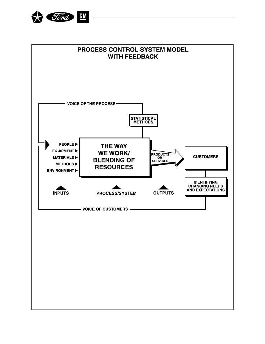
Figure 1. A Process Control System

- 6 -

I. INTRODUCTION TO CONTINUAL IMPROVEMENT AND STATISTICAL PROCESS CONTROL

Section 2

A PROCESS CONTROL SYSTEM

A process control system can be described as a feedback system. Statistical Process Control (SPC) is one
type of feedback system. Other such systems, which are not statistical, also exist. Four elements of that
system are important to the discussions that will follow:

The Process – By the process, we mean the whole combination of suppliers, producers, people,
equipment, input materials, methods, and environment that work together to produce output,
and the customers who use that output (see Figure 1). The total performance of the process
depends upon communication between supplier and customer, the way the process is designed
and implemented, and on the way it is operated and managed. The rest of the process control
system is useful only if it contributes either to maintaining a level of excellence or to improving
the total performance of the process.

Information About Performance – Much information about the actual performance of the
process can be learned by studying the process output. The most helpful information about the
performance of a process comes, however, from understanding the process itself, and its internal
variability. Process characteristics (such as temperatures, cycle times, feed rates, absenteeism,
turnover, tardiness, or number of interruptions) should be the ultimate focus of our efforts. We
need to determine the target values for those characteristics which result in the most productive
operation of the process, and then monitor how near to or far from those target values we are. If
this information is gathered and interpreted correctly, it can show whether the process is acting
in a usual or unusual manner. Proper actions can then be taken, if needed, to correct the process
or the just-produced output. When action is needed it must be timely and appropriate, or the
information-gathering effort is wasted.

Action on the Process – Action on the process is frequently most economical when taken to
prevent the important characteristics (process or output) from varying too far from their target
values. This maintains the stability and the variation of the process output within acceptable
limits. Such action might consist of changes in the operations (e.g., operator training, changes to
the incoming materials, etc.) or the more basic elements of the process itself (e.g., the equipment –
which may need rehabilitation, how people communicate and relate, or the design of the process
as a whole – which may be vulnerable to changes in shop temperature or humidity). The effect of
actions should be monitored, and further analysis and action should be taken if necessary.

Action on the Output – Action on the output is frequently least economical when it is re-
stricted to detecting and correcting out-of-specification product without addressing the underly-
ing process problem. Unfortunately, if current output does not consistently meet customer re-
quirements, it may be necessary to sort all products and to scrap or rework any nonconforming
items. This must continue until the necessary corrective action on the process has been taken
and verified, or until the product specifications have been changed.

It is obvious that inspection followed by action only on the output is a poor substitute for effective process
management. Action only on the output should be used strictly as an interim measure for unstable or
incapable processes (see Section 5). Therefore, the discussions that follow focus on gathering process infor-
mation and analyzing it so that action can be taken to correct the process itself.

- 7 -

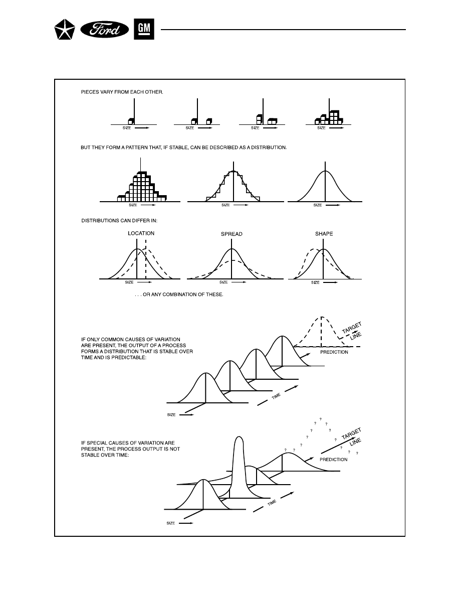
Figure 2. Variation: Common and Special Causes

- 8 -

I. INTRODUCTION TO CONTINUAL IMPROVEMENT AND STATISTICAL PROCESS CONTROL

Section 3

VARIATION: COMMON AND SPECIAL CAUSES

In order to effectively use process control measurement data, it is important to understand the concept of
variation, as illustrated in Figure 2.

No two products or characteristics are exactly alike, because any process contains many sources of vari-
ability. The differences among products may be large, or they may be immeasurably small, but they are
always present. The diameter of a machined shaft, for instance, would be susceptible to potential variation
from the machine (clearances, bearing wear), tool (strength, rate of wear), material (diameter, hardness),
operator (part feed, accuracy of centering), maintenance (lubrication, replacement of worn parts), and
environment (temperature, constancy of power supply). For another example, the time required to process
an invoice could vary according to the people performing various steps, the reliability of any equipment
they were using, the accuracy and legibility of the invoice itself, the procedures followed, and the volume of
other work in the office.

Some sources of variation in the process cause short-term, piece-to-piece differences – e.g., backlash and
clearances within a machine and its fixturing, or the accuracy of a bookkeeper’s work. Other sources of
variation tend to cause changes in the output only over a longer period of time, either gradually as with
tool or machine wear, step-wise as with procedural changes, or irregularly, as with environmental changes
such as power surges. Therefore, the time period and conditions over which measurements are made will
affect the amount of the total variation that will be present.

From the standpoint of minimum requirements, the issue of variation is often simplified: parts within
specification tolerances are acceptable, parts beyond specification tolerances are not acceptable; reports on
time are acceptable, late reports are not acceptable. However, to manage any process and reduce variation,
the variation must be traced back to its sources. The first step is to make the distinction between common
and special causes of variation.

While individual measured values may all be different, as a group they tend to form a pattern that can be
described as a distribution (see Figure 2). This distribution can be characterized by:

• Location (typical value)

• Spread (span of values from smallest to largest)

• Shape (the pattern of variation – whether it is symmetrical, skewed, etc.)

Common causes refer to the many sources of variation within a process that has a stable and repeatable
distribution over time. This is called “in a state of statistical control,” “in statistical control,” or sometimes
just “in control.” Common causes behave like a stable system of chance causes. If only common causes of
variation are present and do not change, the output of a process is predictable.

Special causes (often called assignable causes) refer to any factors causing variation that are not always
acting on the process. That is, when they occur, they make the (overall) process distribution change. Unless
all the special causes of variation are identified and acted upon, they will continue to affect the process
output in unpredictable ways. If special causes of variation are present, the process output is not stable
over time.

The changes in the process distribution due to special causes can either be detrimental or beneficial. When
detrimental, they need to be identified and removed. When beneficial, they should be identified and made a
permanent part of the process. With some mature processes (i.e., processes which have undergone several cycles
of continual improvement), the customer may give special allowance to run a process with a consistently occur-
ring special cause. Such allowances will usually require that the process control plans can assure conformance to
customer requirements and protect the process from other special causes (See Section 5).

- 9 -

LOCAL ACTIONS AND ACTIONS ON THE SYSTEM

- 10 -

Local Actions

•

Are usually required to eliminate special causes of variation

•

Can usually be taken by people close to the process

•

Can correct typically about 15% of process problems

Actions on the System

•

Are usually required to reduce the variation due to common causes

•

Almost always require management action for correction

•

Are needed to correct typically about 85% of process problems

I. INTRODUCTION TO CONTINUAL IMPROVEMENT AND STATISTICAL PROCESS CONTROL

Section 4

LOCAL ACTIONS AND ACTIONS ON THE SYSTEM

There is an important connection between the two types of variation just discussed and the types of action
necessary to reduce them.*

Simple statistical process control techniques can detect special causes of variation. Discovering a special
cause of variation and taking the proper action is usually the responsibility of someone who is directly
connected with the operation. Although management must sometimes be involved to correct the condition,
the resolution of a special cause of variation usually requires local action. This is especially true during the
early process improvement efforts. As one succeeds in taking the proper action on special causes, those
that remain will often require management action, rather than local action.

These same simple statistical techniques can also indicate the extent of common causes of variation, but
the causes themselves need more detailed analysis to isolate. The correction of these common causes of
variation is usually the responsibility of management. Sometimes people directly connected with the op-
eration will be in a better position to identify them and pass them on to management for action. Overall,
though, the resolution of common causes of variation usually requires action on the system.

Only a relatively small proportion of excessive process variation – industrial experience suggests about
15% – is correctable locally by people directly connected with the operation. The majority – the other 85%
– is correctable only by management action on the system. Confusion about the type of action to take is
very costly to the organization, in terms of wasted effort, delayed resolution of trouble, and aggravated
problems. It may be wrong, for example, to take local action (e.g., adjusting a machine) when management
action on the system is required (e.g., selecting suppliers that provide consistent input materials).** Nev-
ertheless, close teamwork between management and those persons directly connected with the operation
is a must for enhancing reduction of common causes of process variation.

Dr. W. E. Deming has treated this issue in “What Happened in Japan?,” Industrial Quality Control,
Vol. 24, No. 3, August, 1967, pages 89-93, and in other articles.

* * These observations were first made by Dr. J. M. Juran, and have been borne out in Dr. Deming’s

experience.

- 11 -

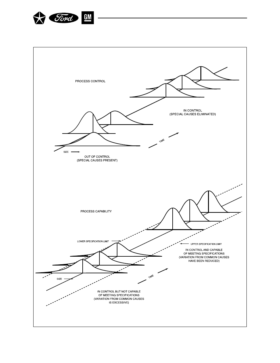
Figure 3. Process Control and Process Capability

- 12 -

I. INTRODUCTION TO CONTINUAL IMPROVEMENT AND STATISTICAL PROCESS CONTROL

Section 5

PROCESS CONTROL AND PROCESS CAPABILITY

The goal of a process control system is to make economically sound decisions about actions affecting the
process. This means balancing the consequences of taking action when action is not necessary (overcontrol
or “tampering”) versus failing to take action when action is necessary (undercontrol). These risks must be
handled, however, in the context of the two sources of variation previously mentioned – special causes and
common causes. (See Figure 3.)

A process is said to be operating in statistical control when the only sources of variation are from common
causes. One function of a process control system, then, is to provide a statistical signal when special causes
of variation are present, and to avoid giving false signals when they are not present. This allows appropri-
ate action(s) to be taken upon those special causes (either removing them or, if they are beneficial, making
them permanent).

When discussing process capability, two somewhat contrasting concepts need to be considered:

•

Process capability is determined by the variation that comes from common causes. It generally
represents the best performance (i.e., minimum spread) of the process itself, as demonstrated
when the process is being operated in a state of statistical control while the data are being col-
lected, irrespective of where the specifications may be with respect to the process location and/or
spread.

•

Customers, however, internal or external, are more typically concerned with the overall output of
the process and how it relates to their requirements (defined as specifications), irrespective of the
process variation.

In general, since a process in statistical control can be described by a predictable distribution, the propor-
tion of in-specification parts can be estimated from this distribution. As long as the process remains in
statistical control and does not undergo a change in location, spread or shape, it will continue to produce
the same distribution of in-specification parts. The first action on the process should be to locate the
process on the target. If the process spread is unacceptable, this strategy allows the minimum number of
out-of-specification parts to be produced. Actions on the system to reduce the variation from common
causes are usually required to improve the ability of the process (and its output) to meet specifications
consistently. For a more specific understanding of the subject of process capability, process performance
and the assumptions associated with it, refer to Chapter II, Section 5.

In short: the process must first be brought into statistical control by detecting and acting upon special
causes of variation. Then its performance is predictable, and its capability to meet customer expectations
can be assessed. This is a basis for continual improvement.

Every process is subject to classification based on capability and control. A process can be classified into 1
of 4 cases, as illustrated by the following chart:

- 13 -

CONTROL

MEETING REQUIREMENTS

NOT IN

CONTROL

ACCEPTABLE

CASE 1

CASE 3

NOT ACCEPTABLE

CASE 2

CASE 4

I. INTRODUCTION TO CONTINUAL IMPROVEMENT AND STATISTICAL PROCESS CONTROL

Section 5. Process Control and Process Capability (Cont.)

To be acceptable, the process must be in a state of statistical control and the inherent variation (capability)
must be less than blueprint tolerance. The ideal situation is to have a Case 1 process where the process is
in statistical control and the ability to meet requirements is acceptable. A Case 2 process is in control but
has excessive common cause variation which must be reduced. A Case 3 process meets requirements ac-
ceptably, but is not in control; special causes of variation must be identified and acted upon. In Case 4, the
process is not in control nor is it acceptable; both common and special cause variation must be reduced.

Under certain circumstances, the customer may allow a producer to run a process even though it is a Case
3 process. These circumstances may include:

• The customer is insensitive to variation within specifications (See discussion on the loss function

in Chapter II, Section 5).

• The economics involved in acting upon the special cause exceed the benefit to any and all custom-

ers. Economically allowable special causes may include tool wear, tool regrind, cyclical (seasonal)
variation, etc.

• The special cause has been identified and has been documented as consistent and predictable.

In these situations, the following may be required by the customer:

• The process is mature; i.e., the process has undergone several cycles of continual improvement.

• The special cause to be allowed has been shown to act in a consistent manner over a known period

of time.

• A process control plan is in effect which will assure conformance to specification of all process

output and protection from other special causes or inconsistency in the allowed special cause.

The accepted practice in the automotive industry is to calculate capability only after a process has been
demonstrated to be in a state of statistical control. Capability is used as a basis for prediction of how the
process will perform using statistical data gathered from a process. There is little value in making predic-
tions based on data collected from a process that is not stable and repeatable over time. Special causes are
responsible for changes in the shape, spread, or location of a process distribution, and thus can rapidly
invalidate capability prediction. The various capability indices and ratios are based, among other things,
on the requirement that data used to calculate them are gathered from processes that are in a state of
statistical control.

Capability indices can be divided into two categories: short-term and long-term. Short-term capability
studies are based on measurements collected from one operating run. The data are analyzed with a control
chart for evidence that the process is operating in a state of statistical control. If no special causes are
found, a short-term capability index can be calculated. If the process is not in control, action regarding the
special cause(s) of variation will be required. This type of study is often used to validate the initial parts
produced from a process for customer submission. Another use, sometimes called a machine capability
study, is to validate that a new or modified process actually performs within the engineering parameters.

When a process has been found to be stable and capable of meeting requirements in the short term, a
different kind of study is subsequently performed. Long-term capability studies consist of measurements
which are collected over a longer period of time. The data should be collected for long enough, and in such
a way, as to include all expected sources of variation. Many of these sources of variation may not have been
observed in the short-term study. When sufficient data have been collected, the data are plotted on a
control chart, and if no special causes are found, long-term capability and performance indices can be
calculated. One use for this study is to describe the ability of the process to satisfy customer requirements
over long periods of time with many possible sources of variation included - i.e., to quantify process performance.

- 14 -

I. INTRODUCTION TO CONTINUAL IMPROVEMENT AND STATISTICAL PROCESS CONTROL

Section 5. Process Control and Process Capability (Cont.)

Several different indices have been developed because 1) no single index can be universally applied to all
processes, and 2) no given process can be completely described by a single index. For example, it is recom-
mended that C

and C

both be used (see Chapter II, Section 5), and further that they be combined with

graphical techniques to better understand the relationship between the estimated distribution and the
specification limits. In one sense, this amounts to comparing (and trying to align) the “voice of the process”
with the “voice of the customer” (see also Reference 22).

All indices have weaknesses and can be misleading. Any inferences drawn from computed indices should
be driven by appropriate interpretation of the data from which the indices were computed.

Automotive companies have set requirements for process capability. It is the reader’s responsibility to
communicate with their customer and determine which indices to use. In some cases, it might be best to
use no index at all. It is important to remember that most capability indices include the product specifica-
tion in the formula. If the specification is inappropriate, or not based upon customer requirements, much
time and effort may be wasted in trying to force the process to conform. Section 5 of Chapter II deals with
selected capability and performance indices and contains advice on the application of those indices.

- 15 -

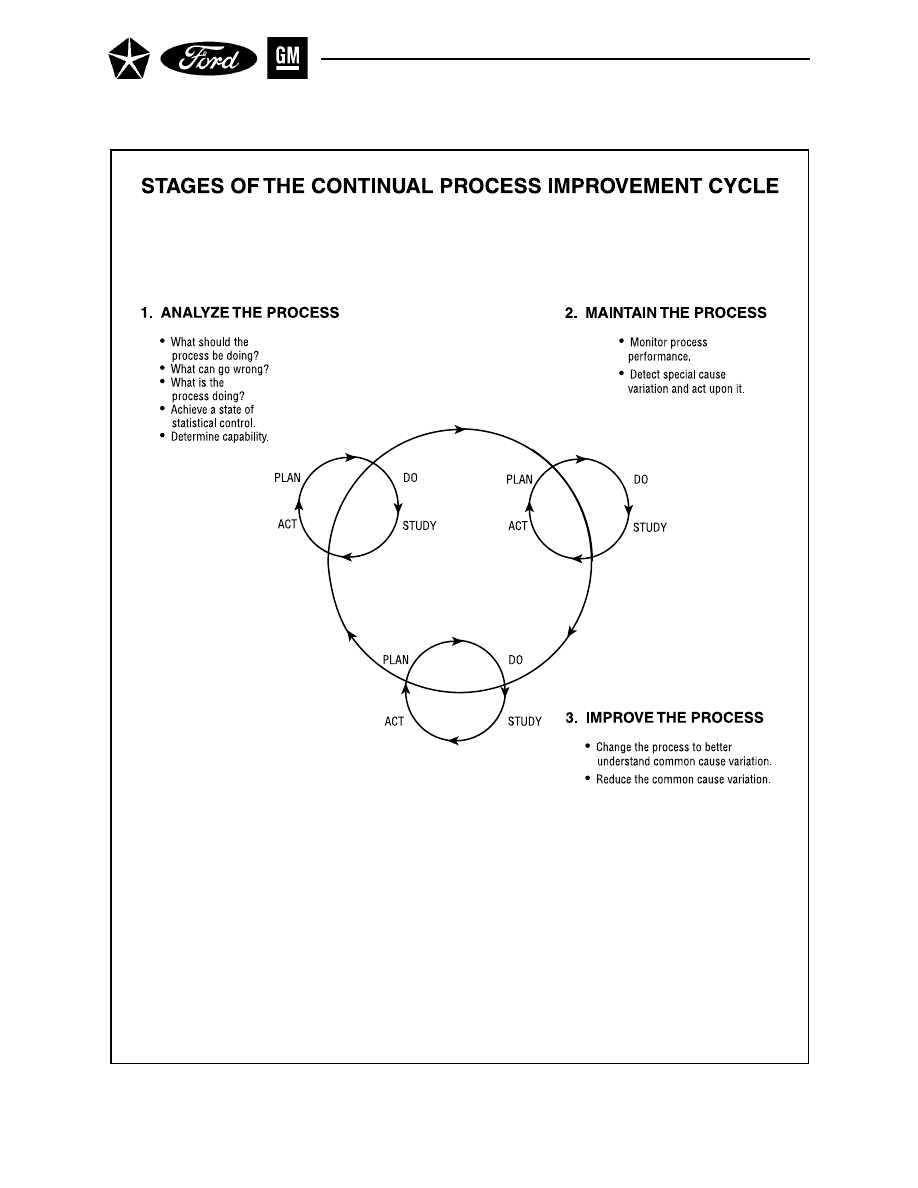
Figure 4. The Process Improvement Cycle

- 16 -

I. INTRODUCTION TO CONTINUAL IMPROVEMENT AND STATISTICAL PROCESS CONTROL

Section 6

THE PROCESS IMPROVEMENT CYCLE AND PROCESS CONTROL

In applying the concept of continual improvement to processes, there is a three stage cycle which can be
useful (see Figure 4). Every process subject to improvement can be located somewhere in this cycle.

1. Analyze the Process

A basic understanding of the process is a must when considering process improvement. Among the ques-
tions to be answered in order to achieve a better understanding of the process are:

• What should the process be doing?

• What can go wrong?

– What can vary in this process?

– What do we already know about this process’s variability?

– What parameters are most sensitive to variation?

• What is the process doing?

– Is this process producing scrap or output which requires rework?

– Does this process produce an output which is in a state of statistical control?

– Is the process capable?

– Is the process reliable?

Many techniques may be applied to gain a better understanding of the process, such as group meetings,
consultation with people who develop or operate the process (“subject matter experts”), review of the process’s
history or construction of a Failure Modes and Effects Analysis (FMEA). Control charts explained in this
manual are powerful tools that should be used. These simple statistical methods help differentiate be-
tween common and special causes of variation. The special causes of variation must be addressed. When a
state of statistical control has been reached, a capability index may be computed to assist in assessing the
process’s current level of long-term capability.

2. Maintain (Control) the Process

Once a better understanding of the process has been achieved, the process must be maintained at an
appropriate level of capability. Processes are dynamic and will change. The performance of the process
must be monitored so effective measures to prevent undesirable change can be taken. Desirable change
also must be understood and institutionalized. Again, the simple statistical methods explained in this
manual can assist you. Construction and use of control charts and other tools will allow for efficient moni-
toring of the process. When the tool used signals that the process has changed, quick and efficient mea-
sures can be taken to isolate the causes(s) and act upon them.

It is too easy to stop at stage two in the Cycle. It is important to realize that there is a limit to any
company’s resources. Some, perhaps many, processes should be at this stage. However, failure to proceed
to the next stage in this cycle can result in a significant competitive disadvantage. The attainment of
“world class” requires a steady and planned effort to move into the next stage of the Process Improvement Cycle.

- 17 -

I. INTRODUCTION TO CONTINUAL IMPROVEMENT AND STATISTICAL PROCESS CONTROL

Section 6. The Continual Improvement Cycle and Process Control (Cont.)

3. Improve the Process

Up to this point, the effort has been to stabilize the processes and maintain them. However, for some
processes, the customer will be sensitive even to variation within engineering specifications. In these
instances, the value of continual improvement will not be realized until variation is reduced. At this point,
additional process analysis tools, including more advanced statistical methods such as designed experi-
ments and advanced control charts may be useful. Appendix H lists some helpful references for further
study.

Process improvement through variation reduction typically involves purposefully introducing changes
into the process and measuring the effects. The goal is a better understanding of the process, so that the
common cause variation can be further reduced. The intent of this reduction is improved quality at lower
cost.

When new process parameters have been determined, the Cycle shifts back to Analyze the Process. Since
changes have been made, process stability will need to be reconfirmed. The process then continues to move
around the Process Improvement Cycle.

- 18 -

- 19 -

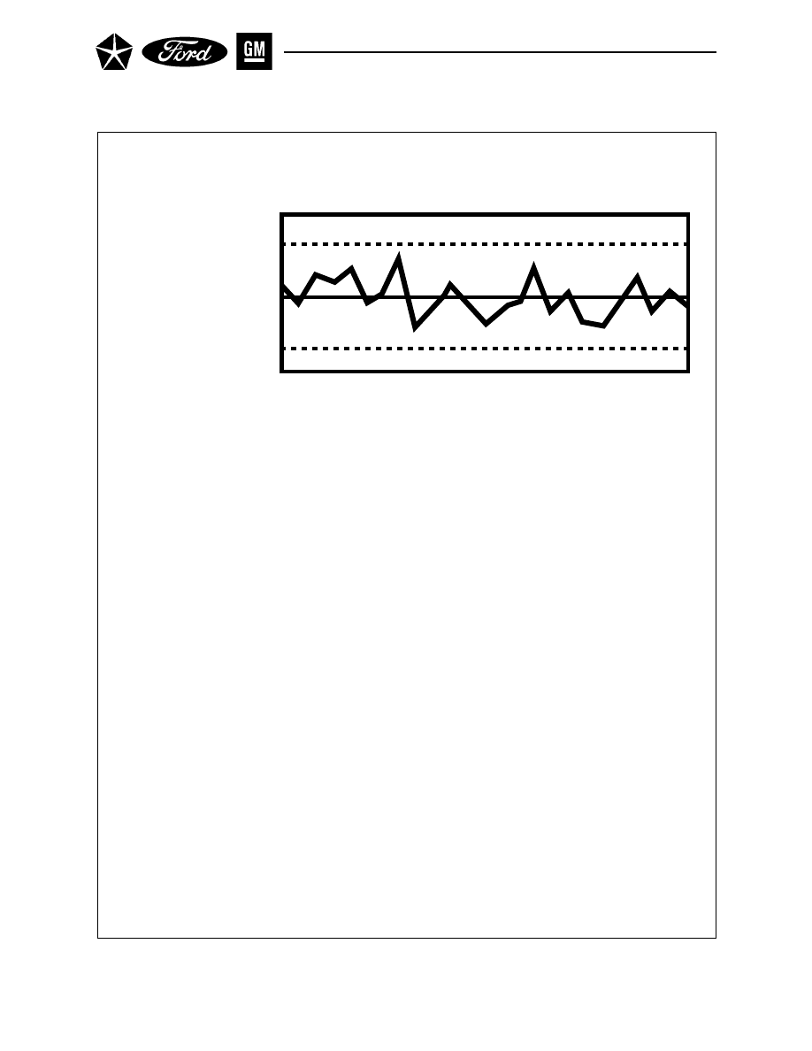
CONTROL CHARTS

Upper Control Limit

Center Line

Lower Control Limit

Collection:

•

Gather data and plot on a chart.

Control:

• Calculate trial control limits from process data.

• Identify special causes of variation and act upon them.

Analysis and Improvement:

• Quantify common cause variation; take action to reduce it.

These three phases are repeated for continual process improvement.

Figure 5. Control Charts

- 20 -

I. INTRODUCTION TO CONTINUAL IMPROVEMENT AND STATISTICAL PROCESS CONTROL

Section 7

CONTROL CHARTS: TOOLS FOR PROCESS CONTROL

Dr. Walter Shewhart of the Bell Laboratories, while studying process data in the 1920’s, first made
the distinction between controlled and uncontrolled variation, due to what we call common and spe-
cial causes. He developed a simple but powerful tool to separate the two – the control chart. Since that
time, control charts have been used successfully in a wide variety of process control situations, both in
the U.S. and other countries, notably Japan. Experience has shown that control charts effectively
direct attention toward special causes of variation when they appear and reflect the extent of common
cause variation that must be reduced by system or process improvement.

Process improvement using control charts is an iterative procedure, repeating the fundamental phases
of collection, control and analysis (see Figure 5). First, data are gathered according to a plan (Appen-
dix A provides input for such a data gathering plan); then, these data are used to calculate control
limits, which are the basis of interpreting the data for statistical control; when the process is in
statistical control, it can be interpreted for process capability. To effect improvements in control and
capability, common and special causes of variation must be identified and the process modified ac-
cordingly; then the cycle begins again, as more data are gathered, interpreted, and used as the basis
for action.

Collection: Data for the characteristic (process or output) being studied are gathered and
converted to a form that can be plotted on a control chart. These data might be the measured
values of a dimension of a machined piece, the number of flaws in a bolt of vinyl, railcar
transit times, number of bookkeeping errors, etc.

Control: Trial control limits are calculated based on the data. They are drawn on the chart
as a guide to analyses. Control limits are not specification limits or objectives, but are based
on the natural variability of the process and the sampling plan.

The data are then compared with the control limits to see whether the variation is stable and
appears to come only from common causes. If special causes of variation are evident, the
process is studied to further determine what is affecting it. After actions (usually local) have
been taken, further data are collected, control limits are recalculated if necessary, and any
additional special causes are acted upon.

Analysis and Improvement: After all special causes have been addressed and the process
is running in statistical control, the control chart continues as a monitoring tool. Process
capability can also be calculated. If the variation from common causes is excessive, the pro-
cess cannot produce output that consistently meets customer requirements. The process itself
must be investigated, and, typically, management action must be taken to improve the system.

- 21 -

I. INTRODUCTION TO CONTINUAL IMPROVEMENT AND STATISTICAL PROCESS CONTROL

Section 7. Control Charts: Tools for Process Control (Cont.)

Often, it is found that although the process was aimed at the target value during initial setup,
the actual process location ( X ) may not match this value. For those processes where the actual
location deviates from the target and the ability to relocate the process is economical, consider-
ation should be given to adjusting the process so that it is better aligned with the target. This
assumes that this adjustment does not affect the process variation. This may not always hold
true, but the causes for any possible increase in process variation after re-targeting the process
should be understood and assessed against both customer satisfaction and economics.

The long-term performance of the process must continue to be analyzed. This is most easily
accomplished by a periodic and systematic review of the on-going control charts. New evidence of
special causes will usually be revealed. Some, when understood, will be beneficial in reducing the
overall process variability. Others, detrimental to the process, will need to be understood and
corrected or removed.

For a process which is “in control,” improvement efforts will often focus on reducing the common
cause variation in the process. Reducing this variation will have the effect of “shrinking” the
control limits on the control chart – i.e., the limits, upon their recalculation, will be closer to-
gether. Many people, not familiar with control charts, feel this is “penalizing” the process for
improving. They do not realize that if a process is stable and the control limits are calculated
correctly, the chance that the process will erroneously yield an out-of-control point is the same
regardless of the distance between the control limits (see also Section 5).

One area deserving mention is the question of recalculation of control chart limits. Once properly
computed, and if no changes to the common cause variation of the process occur, then the control
limits remain legitimate. Signals of special causes of variation do not require the recomputation
of control limits. For long-term analysis of control charts, it is best to recalculate control limits as
infrequently as possible, but as dictated by the process.

For continual process improvement, repeat these three phases. Gather more data as appropriate; work to
reduce process variation by operating the process in statistical control; and, continue to analyze the pro-
cess variability.

- 22 -

- 23 -

BENEFITS OF CONTROL CHARTS

Properly used, control charts can:

•

Be used by operators for ongoing control of a process

•

Help the process perform consistently, predictably, for quality and cost

•

Allow the process to achieve

–

Higher quality

–

Lower unit cost

–

Higher effective capability

•

Provide a common language for discussing the performance of the
process

•

Distinguish special from common causes of variation, as a guide to
local action or action on the system.

- 24 -

I. INTRODUCTION TO CONTINUAL IMPROVEMENT AND STATISTICAL PROCESS CONTROL

Section 8

BENEFITS OF CONTROL CHARTS

The following list summarizes some of the important benefits that can come from using control charts:

• Control charts are effective tools to understand process variation and help achieve statistical con-

trol. They often lend themselves to being maintained at the job station by the operator. They give
the people closest to the operation reliable information on when action should be taken – and on
when action should not be taken (e.g., overadjustment – see Appendix B).

• When a process is in statistical control, its performance will be predictable. Thus both producer

and customer can rely on consistent quality levels, and both can rely on stable costs of achieving
that quality level.

• A process in statistical control can be further improved through reduction of common cause varia-

tion and improved process centering (targeting). The expected effects of proposed improvements in
the system can be anticipated, and the actual effects of even relatively subtle changes can be
identified through the control chart data. The amount of data required will vary with the process
under examination. Such process improvements may reduce cost and improve productivity by
decreasing the variation around the target value.

• Control charts provide a common language for communicating information about the performance

of a process – between the two or three shifts that operate a process;. between line production
(operator, supervisor) and support activities (maintenance, material control, process engineering,
quality control); between different stations in the process; between supplier and user; between the
manufacturing/assembly plant and the design engineering activity.

• Control charts, by distinguishing special from common causes of variation, give a good indication

of whether any problems are likely to be correctable locally or will require management action.
This minimizes the confusion, frustration, and excessive cost of misdirected problem-solving ef-
forts.

The remainder of this manual describes techniques involved in constructing and interpreting control charts.
While reading these technical instructions and recommendations, it is well to keep in mind the real ben-
efits that can come if the control chart approach is mastered and effectively used. For additional assistance
relative to which control chart should be used for which situation, a control chart selection diagram is
provided in Appendix C.

NOTE:

Two sample blank control chart and process log forms are shown in Appendix I. If charts
other than these are used, the following minimum information should be on them: process char-
acteristic name; part number; characteristic description; measurement unit; zero = _____ (for
coded data); frequency of sample; sample size; scale description (x-bar, median, etc.); scale
values; subgroup data, time, operator initials or identification; gage or measurement method
used; a place to log process notes.

It might also be a good idea to include gage repeatability and reproducibility (GR&R%)
information on each chart for added consideration in chart interpretation and to reinforce
the fact that an analysis of the measurement system has been performed.

- 25 -

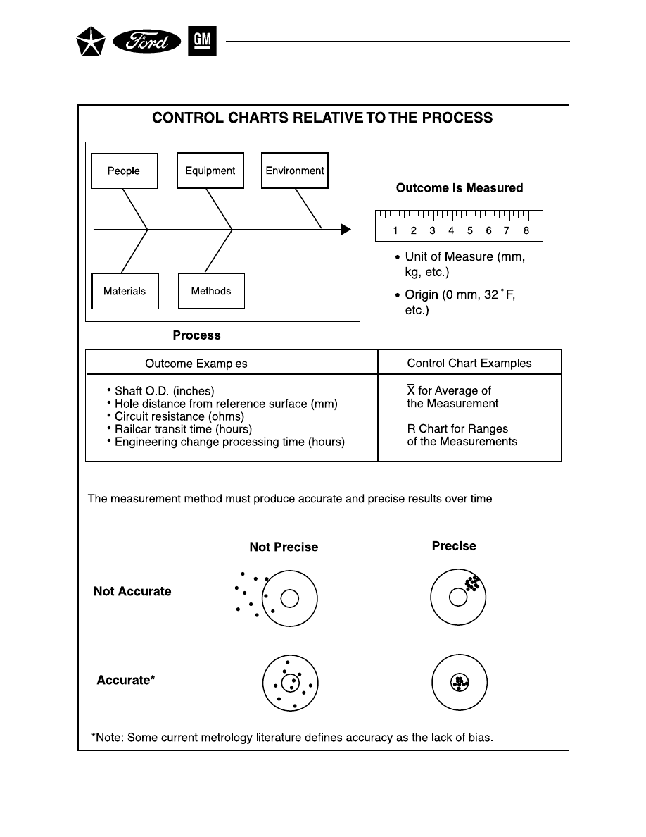
Figure 6. Variables Data – Results from Measuring Intermediate or Final Process Outcome

- 26 -

Chapter II

CONTROL CHART FOR VARIABLES

Control charts for variables are powerful tools that can be used when measurements from a process are
available. Examples would be the diameter of a bearing, the closing effort of a door, or the time to review a
voucher. Variables charts – and especially their most common forms, the X

–

(x bar) and R charts – represent

the typical application of control charting to process control. (See Figure 6.)

Control Charts for variables are particularly useful for several reasons:

Most processes and their outputs have characteristics that are measurable, so the potential ap-
plicability is broad.

A quantitative value (e.g., “the diameter is 16.45 mm”) contains more information than a simple
yes-no statement (e.g., “the diameter is within specification”).

Although obtaining one piece of measured data is generally more costly than obtaining one piece
of go/no-go data, fewer pieces need to be checked to get more information about the process, so in
some cases total measurement costs can be lower.

Because fewer pieces need to be checked before making reliable decisions, the time gap between
production of parts and corrective action often can be shortened.

With variables data, performance of a process can be analyzed, and improvement can be quanti-
fied, even if all individual values are within the specification limits; this is important in seeking
never-ending improvement.

Variables charts can explain process data in terms of both its spread (piece-to-piece variability) and its
location (process average). Because of this, control charts for variables should always be prepared and
analyzed in pairs – one chart for location and another for spread. The most commonly used pair are the X

–

and R charts. X

–

is the average of the values in small subgroups – a measure of location; R is the range of

values within each subgroup (highest minus lowest) – a measure of spread.

The X

–

and R charts are discussed at length in Section 1 of this chapter. Section 2 of this chapter treats X

–

and s charts (an alternative to the R chart), Section 3 treats median charts (a simpler substitute for
average and range charts), and Section 4 of this chapter treats charts for individuals (when decisions must
be based on single readings, not subgroups).

- 27 -

PREPARATION FOR USE OF CONTROL CHARTS

- 28 -

•

Establish an environment suitable for action

•

Define the process

•

Determine characteristics to be managed

Considerations:

– The customer’s needs

– Current and potential problem areas

– Correlation between characteristics

•

Define the measurement system

•

Minimize unnecessary variation

II. CONTROL CHARTS FOR VARIABLES

Section 1

AVERAGE AND RANGE CHARTS ( X

–

AND R)

Before X

–

and R charts can be used, several preparatory steps must be taken:

• Establish an environment suitable for action. Any statistical method will fail unless man-

agement has prepared a responsible environment. Fear within the organization that inhibits people
from being candid must be removed. Management must provide resources to participate in and
support improvement actions.

• Define the process. The process must be understood in terms of its relationship to other opera-

tions and users both upstream and downstream, and in terms of the process elements (people,
equipment, material, methods and environment) that affect it at each stage. Techniques such as
the cause-and-effect diagram and the process flow diagram help make these relationships visible
and allow the pooling of experience from people who understand different aspects of the process.

• Determine characteristics to be charted. One example of a process designed to determine

these characteristics is G.M.’s Key Characteristics Designation System (see Appendix H, Refer-
ence 24). Study efforts should be concentrated on those characteristics that are most promising for
process improvement (an application of the Pareto principle). Several considerations are appropriate:

– The customer’s needs: This includes both any subsequent processes that use the product or

service as an input, and the final end-item customer. Communication of the needs of both types
of customer to the point in the process where improvement can occur takes teamwork and
understanding.

– Current and potential problem areas: Consider existing evidence of waste or poor performance

(e.g., scrap, rework, excessive overtime, missed targets) and areas of risk (e.g., upcoming changes
to the design of the product or service, or to any elements of the process). These are opportuni-
ties for improvement, requiring application of all the disciplines involved in running the business.

– Correlation between characteristics: For an efficient and effective study, take advantage of rela-

tionships among characteristics. For instance, if the characteristic of concern is difficult to mea-
sure (e.g., volume), track a correlated characteristic that is easier to measure (e.g., weight).
Also, if several individual characteristics on an item tend to vary together, it may be sufficient to
chart only one of them. Warning: Statistical correlation does not necessarily imply a cause and
effect relationship between variables. In the absence of existing process knowledge, a designed
experiment may be needed to verify such relationships and their significance.

• Define the measurement system. The characteristic must be operationally defined, so that

findings can be communicated to all concerned in ways that have the same meaning today as
yesterday. This involves specifying what information is to be gathered, where, how, and under
what conditions. The measurement equipment itself must be predictable for bothaccuracy and
precision – periodic calibration is not enough. For more detail on this subject see Section IV. The
definition of the characteristic will affect the type of control chart to be used-a variables data chart,
such as X

–

and R, or an attributes data chart, as described in Section III.

• Minimize unnecessary variation. Unnecessary external causes of variation should be reduced

before the study begins. This could simply mean watching that the process is being operated as
intended, or it could mean conducting a controlled study with known input materials, constant
control settings, etc. The purpose is to avoid obvious problems that could and should be corrected
even without use of control charts; this includes excessive process adjustment or overcontrol. In all
cases, a process log should be kept noting all relevant events such at tool changes, new raw mate-
rial lots, etc. This will aid in subsequent process analysis.

- 29 -

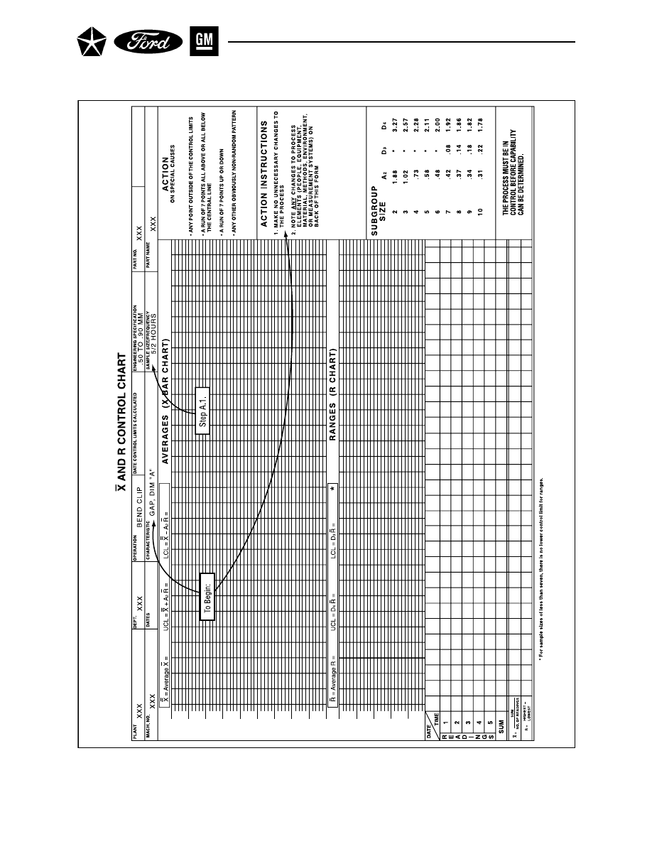
Figure 7. X

–

and R Chart

- 30 -

II. CONTROL CHARTS FOR VARIABLES

Section 1. X and R Charts (Cont.)

A. GATHER DATA

An X

–

and an R chart, as a pair, are developed from measurements of a particular characteristic of the

process output. These data are reported in small subgroups of constant size, usually including from 2 to 5
consecutive pieces, with subgroups taken periodically, (e.g., once every 15 minutes, twice per shift, etc.). A
data gathering plan must be developed and used as the basis for collecting, recording and plotting the data
on a chart.

A.1.

Select the Size, Frequency and Number of Subgroups (See Figure 7.)

Subgroup Size – The first key step in variables control charting is the determination of
“rational subgroups” – they will determine the effectiveness and efficiency of the control
chart that uses them.

The subgroups should be chosen so that opportunities for variation among the units within
a subgroup are small. If the variation within a subgroup represents the piece-to-piece vari-
ability over a very short period of time, then any unusual variation between subgroups
would reflect changes in the process that should be investigated for appropriate action.

For an initial study of a process, the subgroups could typically consist of 4 to 5 consecutively
produced pieces representing only a single tool, head, die cavity, etc. (i.e., a single process
stream). The intention is that the pieces within each subgroup would all be produced under
very similar production conditions over a very short time interval with no other systematic
relationship to each other; hence variation within each subgroup would primarily reflect
common causes. When these conditions are not met, the resulting control chart may not
effectively discriminate special causes of variation, or it may exhibit the unusual patterns
noted in paragraphs C.1.a and C.4.c. of this section. Sample sizes must remain constant for
all subgroups.

Subgroup Frequency – The goal is to detect changes in the process over time. Subgroups
should be collected often enough, and at appropriate times, that they can reflect the poten-
tial opportunities for change. Such potential causes of change could be due to workshift
differences or relief operators, warmup trend, material lots, etc.

During an initial process study, the subgroups themselves are often taken consecutively or
at short intervals, to detect whether the process can shift to show other instability over brief
time periods. As the process demonstrates stability (or as process improvements are made),
the time-period between subgroups can be increased. Subgroup frequencies for ongoing
production monitoring could be twice per shift, hourly, or some other feasible rate.

Number of Subgroups – The number of subgroups should satisfy two criteria. From a pro-
cess standpoint, enough subgroups should be gathered to assure that the major sources of
variation have had an opportunity to appear. Generally, 25 or more subgroups containing
about 100 or more individual readings give a good test for stability and, if stable, good
estimates of the process location and spread.

In some cases, existing data may be available which could accelerate this first phase of the
study. However, they should be used only if they are recent and if the basis for establishing
subgroups is clearly understood.

NOTE:

For further understanding of the impact of subgrouping on control chart interpretation, see
Appendix A.

- 31 -

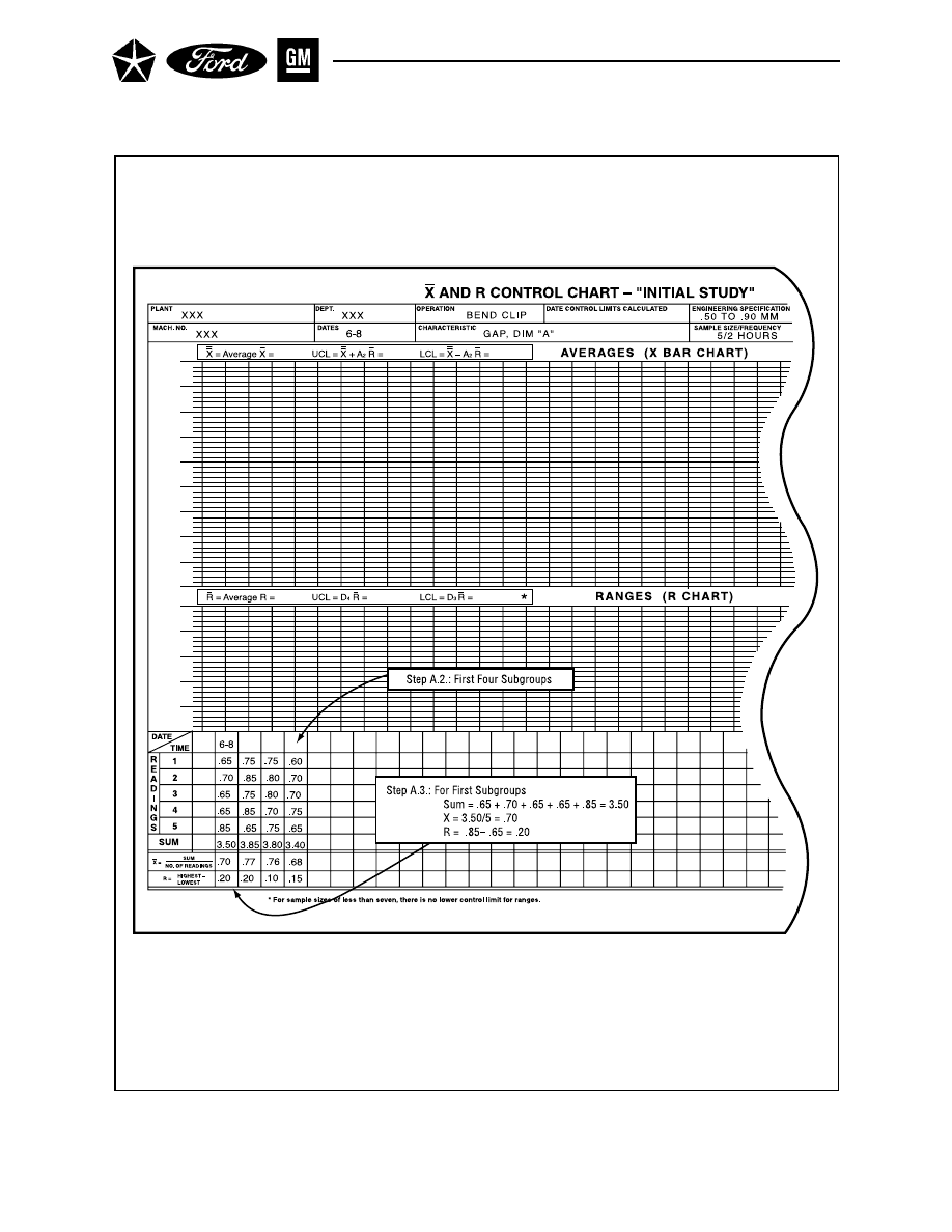
Figure 8. X

–

and R Chart – Setup Data

- 32 -

II. CONTROL CHARTS FOR VARIABLES

Section 1. X and R Charts (Cont.) – Gather Data

A.2.

Set Up Control Charts and Record Raw Data (See Figure 8.)

–

and R charts are normally drawn with the X

–

chart above the R chart, and a data block. The

values of X

–

and R will be the vertical scales, while the sequence of subgroups through time

will be the horizontal scale. The data values and the plot points for the range and average
should be aligned vertically.

The data block should include space for each of the individual readings. It should also in-
clude a space for the sum of the readings, the average ( X

–

), the range (R), and the date/time

or other identification of the subgroup.

Enter the individual values and the identification for each subgroup.

A.3.

Calculate the Average ( X

–

) and Range (R) of Each Subgroup (See Figure 8.)

The characteristics to be plotted are the sample average ( X

–

) and the sample range (R) for

each subgroup; collectively, these reflect the overall process average and its variability, re-
spectively.

For each subgroup, calculate:

–

+ X

+ ... + X

R = X

highest

– X

lowest

where the X

, X

... are individual values within the subgroup and n is the subgroup sample size.

- 33 -

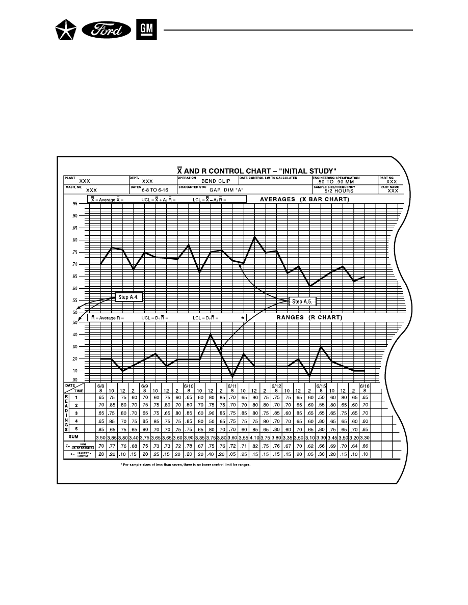
Figure 9. X

–

and R Chart – “Initial Study”

- 34 -

II. CONTROL CHARTS FOR VARIABLES

Section 1. X and R Charts (Cont.) – Gather Data

A.4.

Select Scales for the Control Charts (See Figure 9).

The vertical scales for the two charts are for measured values of X

–

and R respectively. Some

general guidelines for determining the scales may be helpful, although they may have to be
modified in particular circumstances. For the X

–

chart, the difference between the highest and

lowest values on the scale should be at least 2 times the difference between the highest and
lowest of the subgroup averages ( X

–

). For the R chart, values should extend from a lower value of

zero to an upper value about 2 times the largest range (R) encountered during the initial period.

NOTE:

One helpful guide is to set the scale spacing for the range chart to be double that of
the averages chart (e.g., if 1 scale unit equals .01 inches on the averages chart, 1
scale unit would equal .02 inches on the range chart). For typical subgroup sizes,
the control limits for averages and ranges will be about the same width, a visual aid
to analysis.

A.5.

Plot the Averages and Ranges on the Control Charts (See Figure 9).

Plot the averages and ranges on their respective charts. This should be done as soon as possible
after scaling has been decided. Connect the points with lines to help visualize patterns and trends.

Briefly scan the plot points to see if they look reasonable; if any points are substantially higher or
lower than the others, confirm that the calculations and plots are correct. Make sure that the plot
points for the corresponding X

–

and R are vertically in line.

NOTE:

In order to reinforce the practice of all charts on the production floor having control
limits on them, initial run charts which do not yet have control limits calculated
(due to insufficient amounts of data) should be clearly identified “Initial Study”.
Thus, these “Initial Study” charts, whether used for first time capability or for
studies after process improvements/changes, should be the only process control
charts allowed on the production floor which do not have control limits placed on them.

- 35 -

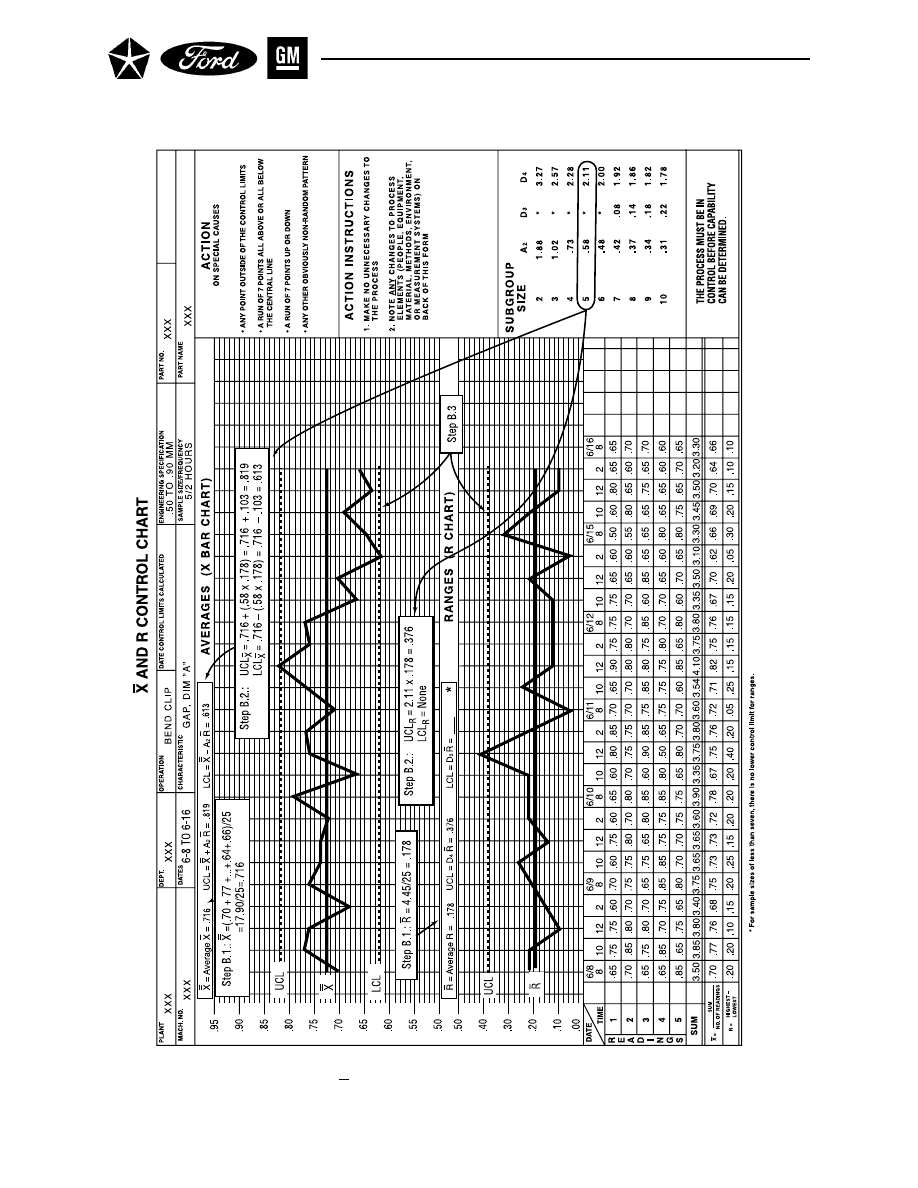
Figure 10. X and R Chart – With Control Limits

- 36 -

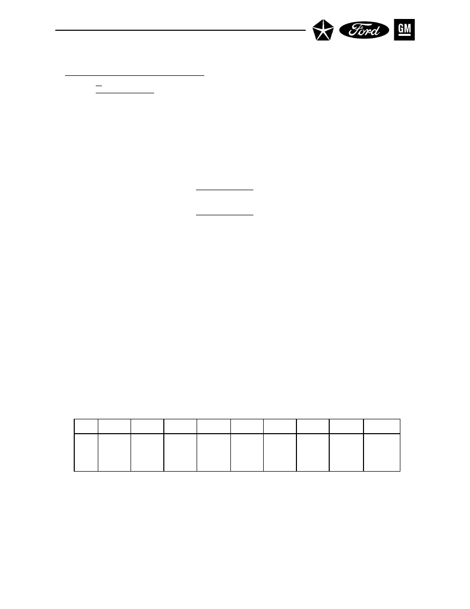
II. CONTROL CHARTS FOR VARIABLES

Section 1. X and R Charts (Cont.)

B. CALCULATE CONTROL LIMITS

Control limits for the range chart are developed first, then those for the chart for averages. The
calculations for the control limits for variables charts use constants which appear as letters in the
formulas that follow. These factors, which differ according to the subgroup size (n), are shown in brief
tables accompanying the respective formulas; more complete tables are shown in Appendix E.

B.1.

Calculate the Average Range (R

–

) and the Process Average ( X

–

) (See Figure 10.)

For the study period, calculate:

R =

+ R

+ ... + R

X =

+ X

+ ... + X

where k is the number of subgroups, R

and X

–

are the range and average of the first subgroup,

R2 and X

–

are from the second subgroup, etc.

B.2.

Calculate the Control Limits (See Figure 10.)

Control limits are calculated to show the extent by which the subgroup averages and ranges
would vary if only common causes of variation were present. They are based on the subgroup
sample size and the amount of within-subgroup variability reflected in the ranges. Calculate the
upper and lower control limits for ranges and for averages:

UCL

= D

–

LCL

= D

–

UCL

–

= X + A

–

LCL

–

= X - A

–

where D

, D

and A

are constants varying by sample size, with values for sample sizes from 2 to 10 as

shown in the following partial table, taken from Appendix E:

* (for sample sizes below 7, the LCL

would technically be a negative number; in those cases there

is no lower control limit; this means that for a subgroup size of 6, six “identical” measurements
would not be unreasonable).

B.3.

Draw Lines for the Averages and the Control Limits on the Charts (See Figure 10.)

Draw the average range ( R

–

) and process average ( X

–

) as solid horizontal lines, the control limits

(UCL

, LCL

, UCL

–

, LCL

–

) as dashed horizontal lines; label the lines. During the initial study

phase,

these are considered trial control limits.

3.27

2.57

2.28

2.11

2.00

1.92

1.86

1.82

1.78

.08

.14

.18

.22

1.88

1.02

.73

.58

.48

.42

.37

.34

.31

- 37 -

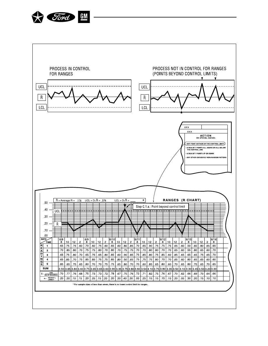
Figure 11. R Chart – Point Beyond Control Limits

- 38 -

II. CONTROL CHARTS FOR VARIABLES

Section 1. X and R Charts (Cont.)

C. INTERPRET FOR PROCESS CONTROL

The control limits can be interpreted as follows: if the process piece-to-piece variability and the process

average were to remain constant at their present levels (as estimated by R

–

and X respectively), the indi-

vidual subgroup ranges (R) and averages ( X

–

) would vary by chance alone, but they would seldom go

beyond the control limits. Likewise, there would be no obvious trends or patterns in the data, beyond what
would likely occur due to chance. The objective of control chart analysis is to identify any evidence that the
process variability or the process average are not operating at a constant level – that one or both are out of
statistical control – and to take appropriate action. The R and X

–

chart are analyzed separately, but com-

parison of patterns between the two charts may sometimes give added insight into special causes affecting
the process.

C.1.

Analyze the Data Plots on the Range Chart

Since the ability to interpret either the subgroup ranges or subgroup averages depends on the
estimate of piece-to-piece variability, the R chart is analyzed first. The data points are compared
with the control limits, for points out of control or for unusual patterns or trends.

Points Beyond the Control Limits (See Figure 11.) – The presence of one or more points
beyond either control limit is primary evidence of non-control at that point. Since points
beyond the control limits would be very rare if only variation from common causes were
present we presume that a special cause has accounted for the extreme value. Therefore,
any point beyond a control limit is the signal for immediate analysis of the operation for the
special cause. Mark any data points that are beyond the control limits for further investiga-
tion and corrective action based on when that special cause actually started. (See para-
graph C.2. Of this section ).

A point above the upper control limit for ranges is generally a sign of one or more of the
following:

• The control limit or plot point has been miscalculated or misplotted.
• The piece-to-piece variability or the spread of the distribution has increased (i.e., wors-

ened), either at that one point in time or as part of a trend.

• The measurement system has changed (e.g., a different inspector or gage).
• The measurement system lacks appropriate discrimination.

A point below the lower control limit (for sample sizes of 7 or more) is generally a sign of one
or more of the following:

• The control limit or plot point is in error.
• The spread of the distribution has decreased (i.e., become better).
• The measurement system has changed (including editing or alteration of the data).

Patterns or Trends Within the Control Limits – The presence of unusual patterns or trends,
even when all ranges are within the control limits, can be evidence of non-control or change
in process spread during the period of the pattern or trend. This could give the first warning
of unfavorable conditions which should be corrected. Conversely, certain patterns or trends
could be favorable and should be studied for possible permanent improvement of the pro-
cess. Comparison of patterns between the range and average charts may give added in-
sight.

- 39 -

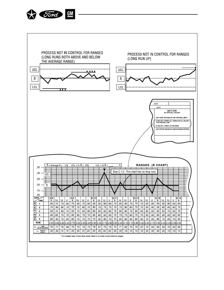
Figure 12. R Chart – Runs (Range)

- 40 -

II. CONTROL CHARTS FOR VARIABLES

Section 1. X and R Charts (Cont.) – Interpret for Control

Runs (See Figure 12.) – Each of the following are signs that a process shift or trend has
begun:

• 7 points in a row on one side of the average.
• 7 points in a row that are consistently increasing (equal to or greater than the preceding

points) or consistently decreasing.

Mark the point that prompts the decision; it may be helpful to extend a reference line back
to the beginning of the run. Analysis should consider the approximate time at which it
appears that the trend or shift first began.

A run above the average range, or a run up signifies one or both of the following:

• Greater spread in the output values, which could be from an irregular cause (such as

equipment malfunction or loose fixturing) or from a shift in one of the process elements
(e.g., a new, less uniform raw material lot); these are usually troubles that need correc-tion.

• A change in the measurement system (e.g., new inspector or gage).

A run below the average range, or a run down signifies one or both of the following:

• Smaller spread in output values, which is usually a good condition that should be stud-

ied for wider application and process improvement.

• A change in the measurement system, which could mask real performance changes.

NOTE: As the subgroup size (n) becomes smaller (5 or less), the likelihood of runs below R

increases, so a run length of 8 or more could be necessary to signal a decrease in
process variability.

- 41 -

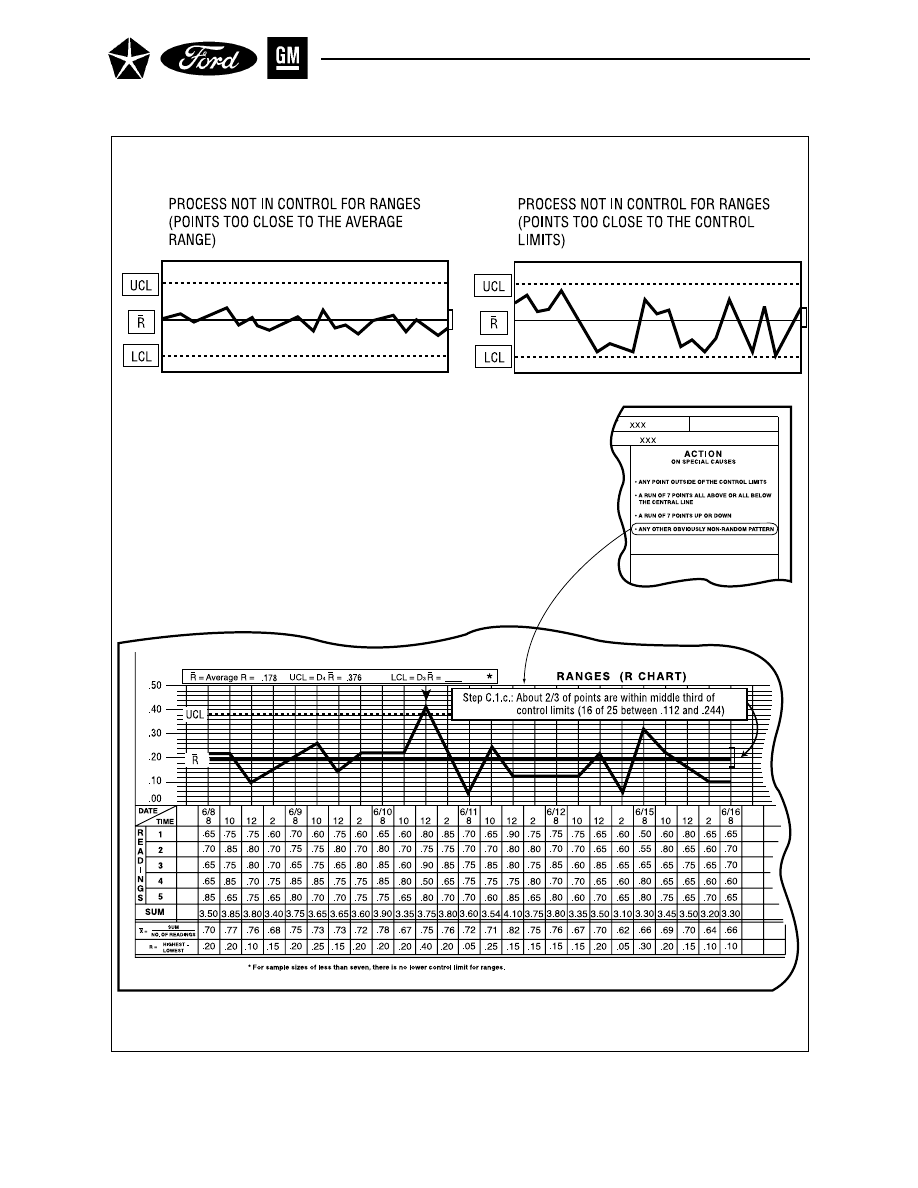
Figure 13. R Chart – Nonrandom Patterns

- 42 -

II. CONTROL CHARTS FOR VARIABLES

Section 1. X and R Charts (Cont.) – Interpret for Control

Obvious Nonrandom Patterns (See Figure 13.) – In addition to the presence of points be-
yond control limits or long runs, other distinct patterns may appear in the data that give
clues to special causes. Care should be taken not to over-interpret the data, since even
random (i.e., common cause) data can sometimes give the illusion of nonrandomness (i.e.,
special causes present). Examples of nonrandom patterns could be obvious trends (even
though they did not satisfy the runs tests), cycles, the overall spread of data points within
the control limits, or even relationships among values within subgroups (e.g., the first read-
ing might always be the highest). One test for the overall spread of subgroup datapoints is
described below:

Distance of points from R

–

: Generally, about 2/3 of the plotted points should lie within the

middle third of the region between the control limits; about 1/3 of the points should be in the
outer two-thirds of the region.

If substantially more than 2/3 of the plotted points lie close to R

–

(for 25 subgroups if over

90% are in the middle third of the control limit region), investigate one or more of the
following:

• The control limits or plot points have been miscalculated or misplotted.
• The process or the sampling method are stratified; each subgroup systematically con-

tains measurements from two or more process streams that have very different process
averages (e.g., one piece from each of several spindles).*

• The data have been edited (subgroups with ranges that deviated much from the average

have been altered or removed).

If substantially fewer than 2/3 of the plotted points lie close to R

–

(for 25 subgroups if 40% or

fewer are in the middle third), investigate one or both of the following:

• The control limits or plot points have been miscalculated or misplotted.
• The process or the sampling method cause successive subgroups to contain measure-

ments from two or more process streams that have dramatically different variability
(e.g., mixed lots of input materials).*

If several process streams are present, they should be identified and tracked separately.*

* See Appendix A.

- 43 -

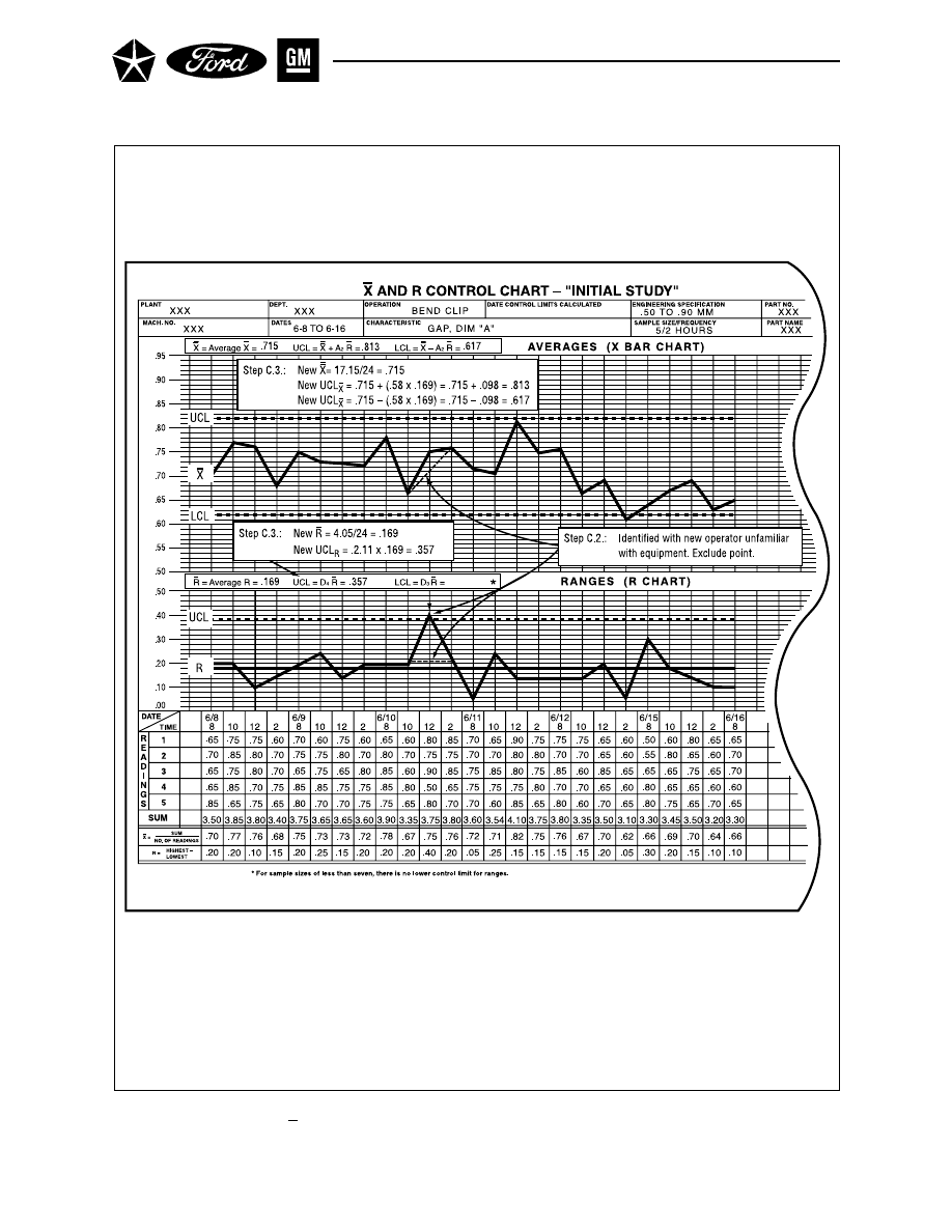
Figure 14. X and R Chart – Control Limits Recalculation (Range)

- 44 -

II. CONTROL CHARTS FOR VARIABLES

Section 1. X and R Charts (Cont.) – Interpret for Control

C.2.

Find and Address Special Causes (Range Chart) (See Figure 14.)

For each indication of a special cause in the range data, conduct an analysis of the operation of the
process to determine the cause and improve process understanding; correct that condition, and
prevent it from recurring. The control chart itself should be a useful guide in problem analysis,
suggesting when the condition began and how long it continued. However, recognize that not all
special causes are negative, that some special causes can result in positive process improvement
in terms of decreased variation in the range – those special causes should be assessed for possible
institutionalization within the process, where appropriate.

Timeliness is important in problem analysis, both in terms of minimizing the production of non-
conforming output, and in terms of having fresh evidence for diagnosis. For instance, the appear-
ance of a single point beyond the control limits is reason to begin an immediate analysis of the
process. A process log may also be a helpful source of information in terms of identifying special
causes of variation.

It should be emphasized that problem solving is often the most difficult and time-consuming
step. Statistical input from the control chart can be an appropriate starting point, but other
methods such as Pareto charts, cause and effect diagrams, or other graphical analysis can be
helpful (see Appendix H, Reference 11). Ultimately, however, the explanations for behavior lie
within the process and the people who are involved with it. Thoroughness, patience, insight and
understanding will be required to develop actions that will measurably improve performance.

C.3.

Recalculate Control Limits (Range Chart) (See Figure 14.)

When conducting an initial process study or a reassessment of process capability, the control
limits should be recalculated to exclude the effects of out-of-control periods for which process
causes have been clearly identified and removed or institutionalized. Exclude all subgroups af-
fected by the special causes that have been identified and removed or institutionalized, then
recalculate and the plot the new average range ( R

–

) and control limits. Confirm that all range

points show control when compared to the new limits, repeating the identification/correction/
recalculation sequence if necessary.

If any subgroups were dropped from the R chart because of identified special causes, they should
also be excluded from the X

–

chart. The revised R

–

and X should be used to recalculate the trial

control limits for averages, X

–

NOTE:

The exclusion of subgroups representing unstable conditions is not just “throwing
away bad data.” Rather, by excluding the points affected by known special causes,
we have a better estimate of the background level of variation due to common
causes. This, in turn, gives the most appropriate basis for the control limits used to
detect future occurrences of special causes of variation. Be reminded, however, that
the process must be changed so the special cause will not recur (if undesireable) as
part of the process.

- 45 -

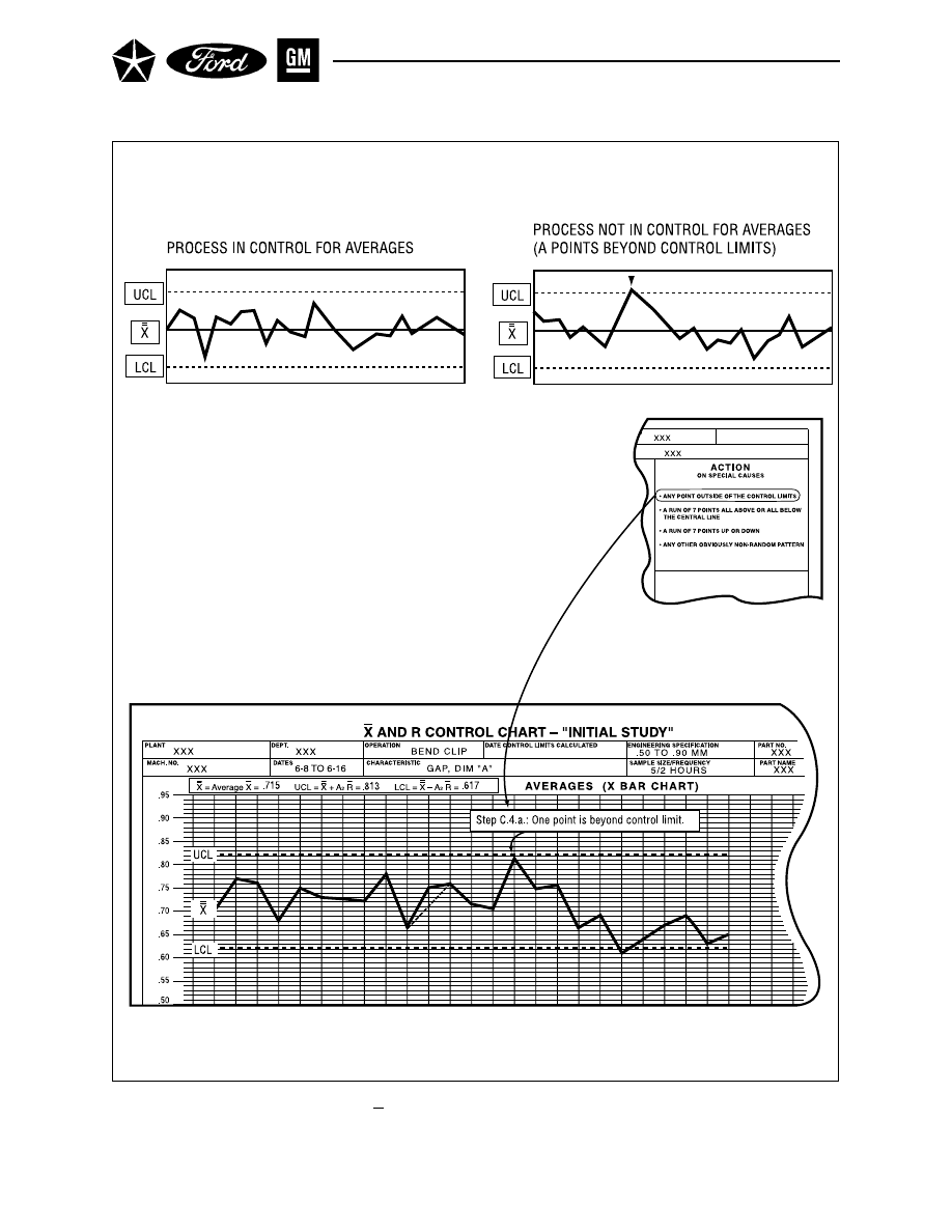
Figure 15. X Chart – Points Beyond Control Limits

- 46 -

II. CONTROL CHARTS FOR VARIABLES

Section 1. X and R Charts (Cont.) – Interpret for Control

C.4.

Analyze the Data Plots on the Averages Chart

When the ranges are in statistical control, the process spread – the within-subgroup variation – is
considered to be stable. The averages can then be analyzed to see if the process location is changing
over time. Since control limits for X-bar are based upon the amount of variation in the ranges, then if
the averages are in statistical control, their variation is related to the amount of variation seen in the
ranges–the common-cause variation of the system. If the averages are not in control, some special
causes of variation are making theprocess location unstable.

Points Beyond the Control Limits (See Figure 15.) – The presence of one or more points beyond
either control limit is primary evidence of the presence of special causes at that point. It is the
signal for immediate analysis of the operation. Mark such data points on the chart (see page 39).

A point beyond either control limit is generally a sign of one or more of the following:

• The control limit or plot point are in error.
• The process has shifted, either at that one point in time (possibly an isolated incident) or as

part of a trend.

• The measurement system has changed (e.g., different gage or inspector).

- 47 -

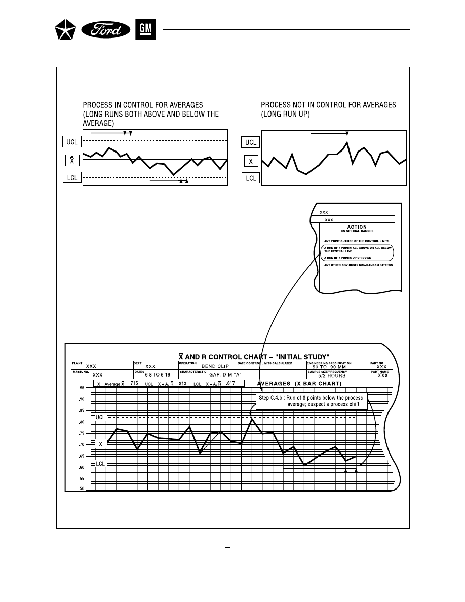
Figure 16. X Chart – Runs

- 48 -

II. CONTROL CHARTS FOR VARIABLES

Section 1. X and R Charts (Cont.) – Interpret for Control

Patterns or Trends Within the Control Limits – The presence of unusual patterns or trends can
be evidence of non-control during the period of the pattern or trend. Comparison of patterns
between the range and average charts may be helpful.

Runs (See Figure 16.) – Each of the following are signs that a process shift or trend has
begun:

• 7 points in a row on one side of the average.
• 7 points in a row that are consistently increasing or decreasing.

Mark the point that prompts the decision; it may help to extend a reference line to the point
at which the run began. Analysis should consider the time at which it appears that the
trend or shift first began.

A run relative to the process average is generally a sign of one or both of the following:

• The process average has changed – and may still be changing.
• The measurement system has changed (drift, bias, sensitivity, etc.).

- 49 -

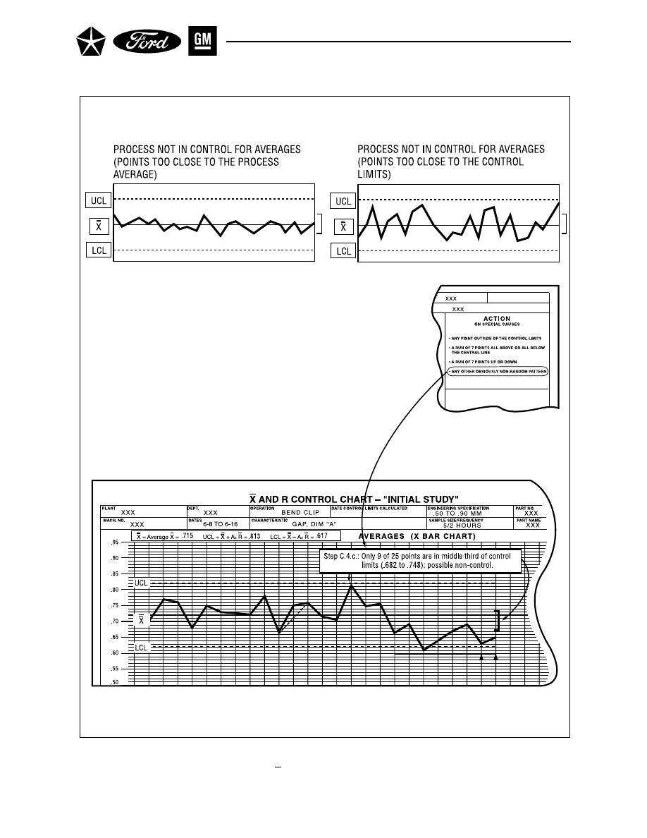
Figure 17. X Chart – Nonrandom Patterns

- 50 -

II. CONTROL CHARTS FOR VARIABLES

Section 1. X and R Charts (Cont.) – Interpret for Control

Obvious Nonrandom Patterns (See Figure 17.) – Other distinct patterns may also indicate the
presence of special causes of variation, although care must be taken not to over-interpret the
data. Among these patterns are trends, cycles, unusual spread of points within the control
limits, and relationships among values within subgroups. One test for unusual spread is given
below:

Distance of points from the process average: Generally, about 2/3 of the plotted points should lie
within the middle third of the region between the control limits; about 1/3 of the points will be in
the outer two-thirds of the region; about 1/20 will lie relatively close to the control limits (in the
outer third of the region). Also, the probability exists that about 1/150 could lie outside control
limits but still be legitimately part of a stable system in control-i.e., only about 99.73% of the
points will be within the control limits.

If substantially more than 2/3 of the points lie close to the process average (for 25 subgroups if
over 90% are in the middle third of the control limit region), investigate one or more of the
following:

• The control limits or plot points have been miscalculated, misplotted, or incorrectly recalcu-

lated.

• The process or the sampling method are stratified; each subgroup contains measurements

from two or more process streams that have different averages.

• The data have been edited.

If substantially fewer than 2/3 of the data points lie close to the process average (for 25 sub-
groups if 40% or fewer are in the middle third), investigate one or both of the following:

• The control limits or plot points have been miscalculated or misplotted.
• The process or the sampling method cause successive subgroups to contain measurements

from two or more very different process streams * (this can be the result of over-control of an
adjustable process, where process changes are made in response to random fluctuations in
the process data**).

If several process streams are present, they should be identified and tracked separately. *

* See example in Appendix A.

**See example in Appendix B.

- 51 -

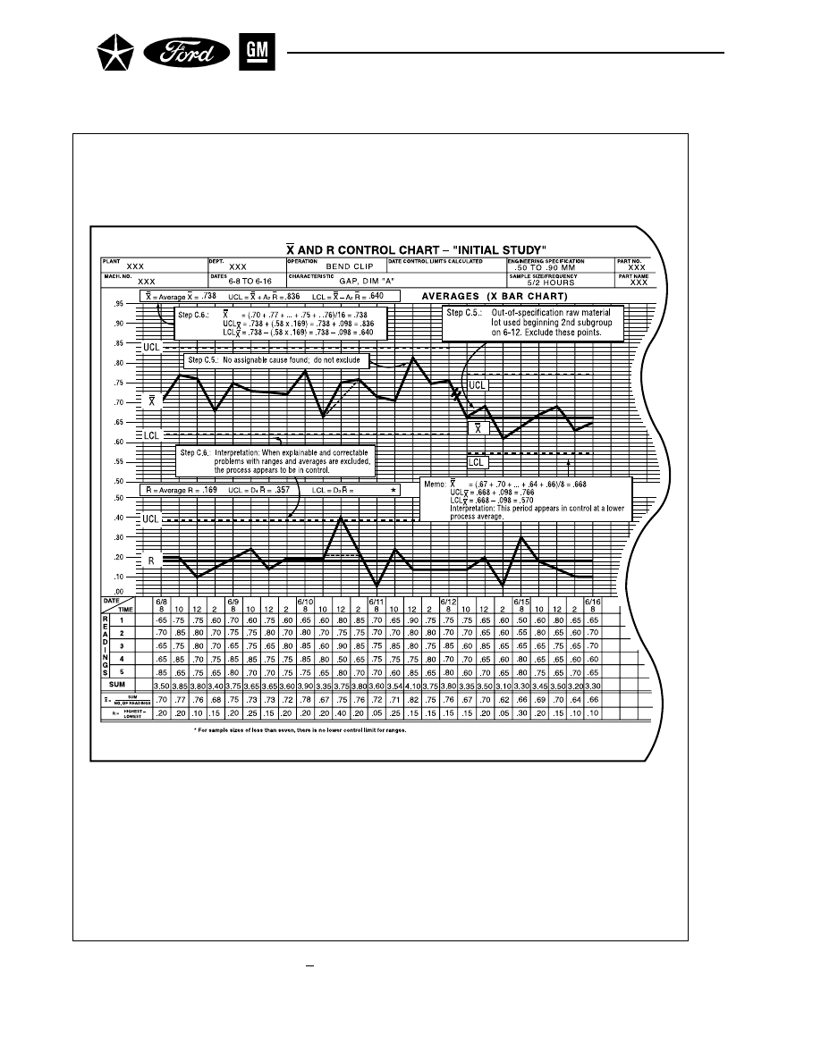
Figure 18. X and R Chart – Control Limits Recalculation

- 52 -

II. CONTROL CHARTS FOR VARIABLES

Section 1. X and R Charts (Cont.) – Interpret for Control

C.5.

Find and Address Special Causes (Averages Chart) (See Figure 18.)

For each indication of an out-of-control condition in the average data, conduct an analysis of the
operation of the process to determine the reason for the special cause; correct that condition, and
prevent it from recurring. Use the chart data as a guide to when such conditions began and how
long they continued. Timeliness in analysis is important, both for diagnosis and to minimize
nonconforming output. Again, be aware that not all special causes need be undesirable (see Page
45, Section C.2).

Problem solving techniques such as Pareto analysis and cause-and-effect analysis can help. (See
Appendix H, Reference 11.)

C.6.

Recalculate Control Limits (Averages Chart) (See Figure 18.)

When conducting an initial process study or a reassessment of process capability, exclude any
out-of-control points for which special causes have been found and removed; recalculate and plot
the process average and control limits. Confirm that all data points show control when compared
to the new limits, repeating the identification/correction/recalculation sequence if necessary.

The preceding discussions were intended to give a functional introduction to control chart analysis. There
are, however, other considerations that can be useful to the analyst. One of the most important is the
reminder that, even with processes that are in statistical control, as more data are reviewed, the constant
chances of getting a false signal of a special cause on any individual subgroup translate to increasing
likelihood of finding false signals somewhere on the chart(s).

While it is wise to investigate all signaled events as possible evidence of special causes, it should be recog-
nized that they may have been caused by the system and that there may be no underlying local process
problem. If no clear evidence of a process special cause is found, any “corrective” action will probably serve
to increase, rather than decrease, the total variability in the process output.

For further discussion of interpretation, tests for randomness in data, and problem-solving, see Appendix
H, References 7-13.

- 53 -

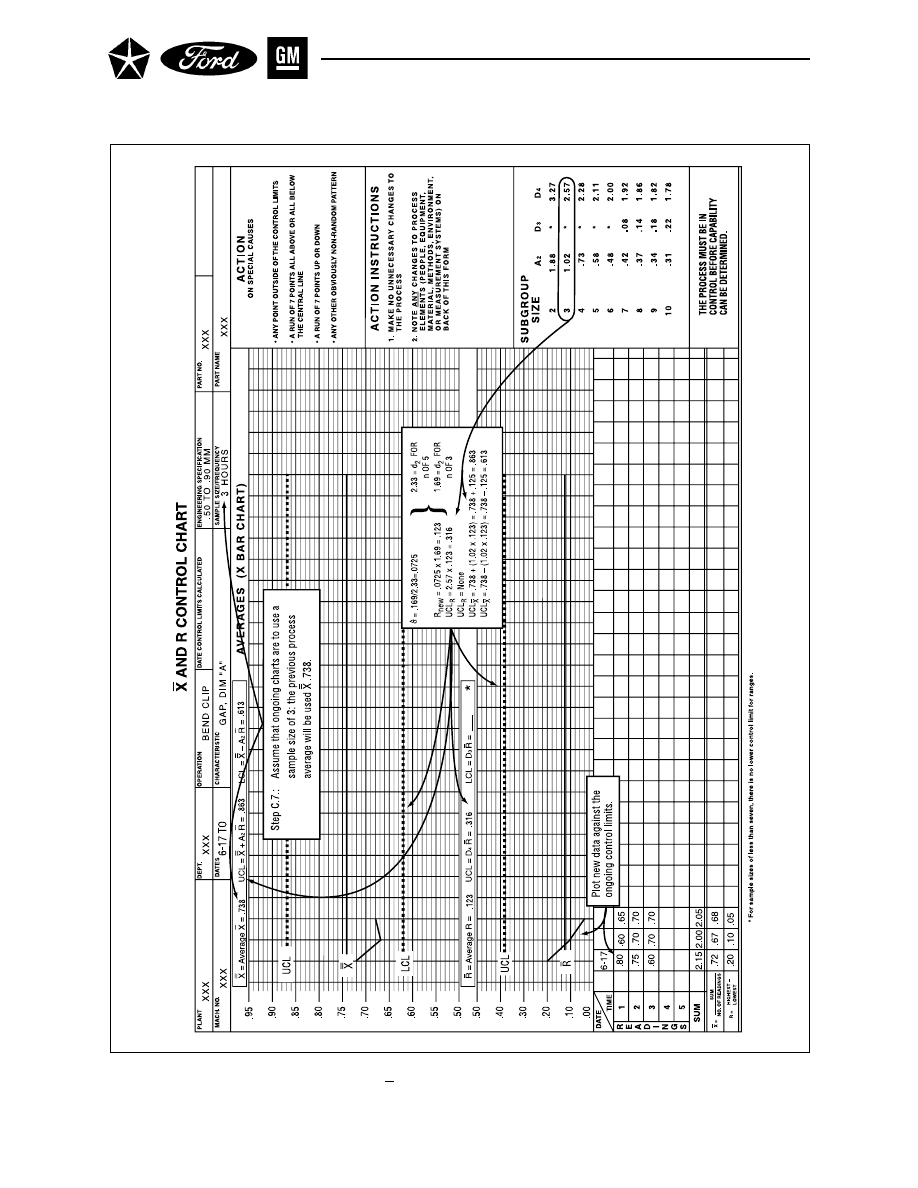
Figure 19. X and R Chart – Extended Limits

- 54 -

II. CONTROL CHARTS FOR VARIABLES

Section 1. X and R Charts (Cont.) – Interpret for Control

C.7.

Extend Control Limits for Ongoing Control (See Figure 19.)

When the initial (or historical) data are consistently contained within the trial control limits,
extend the limits to cover future periods. It might be desirable here to also adjust the process to
the target, if the process center is off target (see page 22). These limits would be used for ongoing
monitoring of the process, with the operator and local supervision responding to signs of out-of-
control conditions on either the X

–

or R chart with prompt action.

A change in the subgroup sample size would affect the expected average range and the control
limits for both ranges and averages. This situation could occur, for instance, if it was decided to
take smaller samples more frequently, so as to detect large process shifts more quickly without
increasing the total number of pieces sampled per day. To adjust central lines and control limits
for a new subgroup sample size, the following steps should be taken:

Estimate the process standard deviation (the estimate is shown as σ

– “sigma hat”). Using

the existing subgroup size calculate: σ

= R

–

where R

–

is the average of the subgroup ranges (for periods with the ranges in control) and

is a constant varying by sample size, as shown in the partial table below, taken from

Appendix E:

Using the tabled factors for d

, D

, and A

based on the new subgroup size, calculate the

new range and control limits:

–

new

= σ

UCL

= D

–

new

LCL

= D

–

new

UCL

= X + A

–

new

LCL

= X – A

new

Plot these new control limits on the chart as the basis for ongoing process control.

As long as the process remains in control for both averages and ranges, the ongoing limits can be
extended for additional periods. If, however, there is evidence that the process average or range
has changed (in either direction), the cause should be determined and, if the change is justifiable,
control limits should be recalculated based on current performance.

C.8.

Final Concepts on “Control” – For Further Consideration

“A perfect state of control is never attainable in a production process. The goal of the process
control charts is not perfection, but a reasonable and economical state of control. For practical
purposes, therefore, a controlled process is not one where the chart never goes out of control. If a
chart never went out of control we would seriously question whether that operation should be
charted. For shop purposes a controlled process is considered to be one where only a small per-
centage of the points go out of control and where out-of-control points are followed by proper
action.” (From Appendix H, Reference 7, page 220-221.)

1.13

1.69

2.06

2.33

2.53

2.70

2.85

2.97

3.08

- 55 -

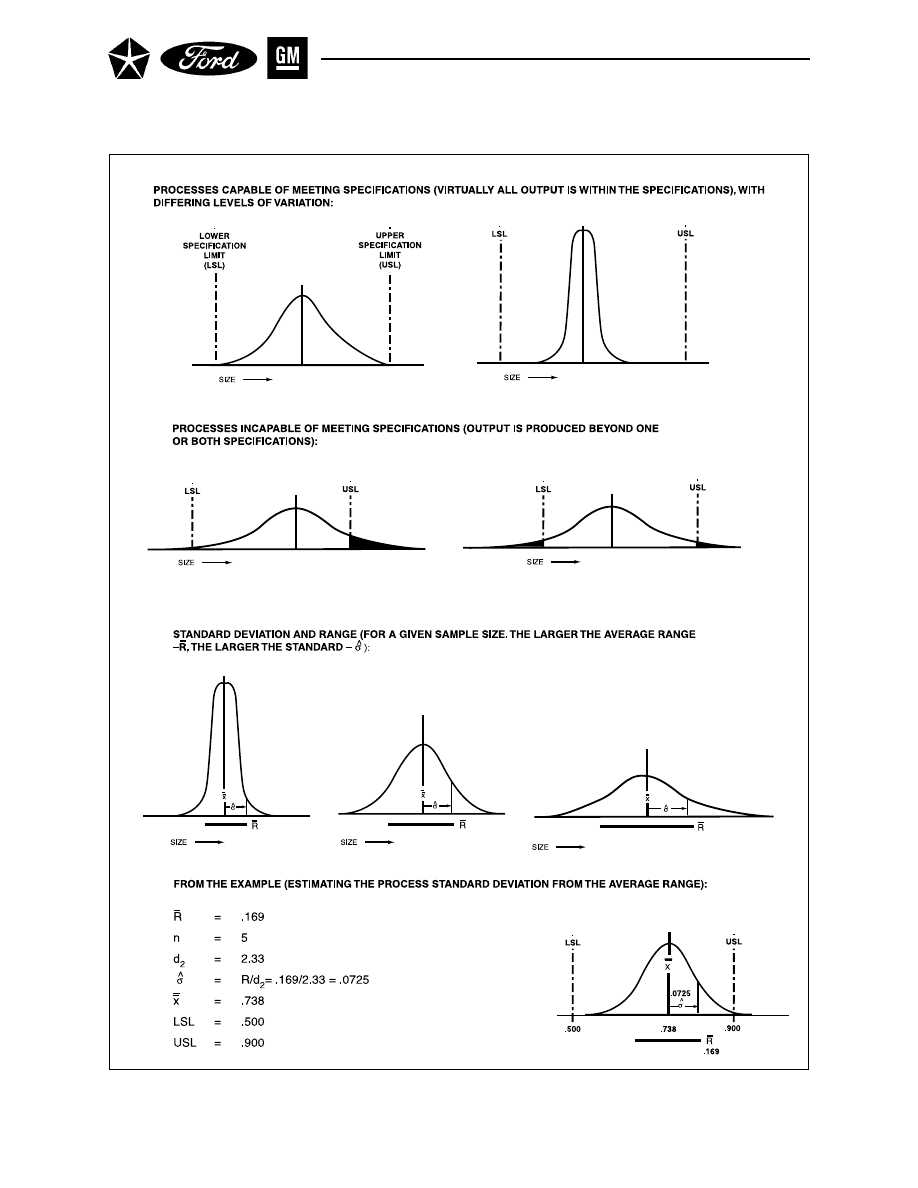
Figure 20. Process Variation Relative To Specification Limits

- 56 -

II. CONTROL CHARTS FOR VARIABLES

Section 1. X and R Charts ( Cont.)

Obviously, there are different levels or degrees of statistical control. The definition of control
used can range from mere outliers (beyond the control limits), through runs, trends and
stratification, to full zone analysis. As the definition of control used advances to full zone
analysis, the likelihood of finding lack of control increases (for example, a process with no
outliers may demonstrate lack of control through an obvious run still within the control
limits). For this reason, the definition of control used should be consistent with your ability
to detect this at the point of control and should remain the same within one time period,
within one process. Some suppliers may not be able to apply the fuller definitions of control
on the floor on a real-time basis due to immature stages of operator training or lack of sophis-
tication in the operator’s ability. The ability to detect lack of control at the point of control on
a real-time basis is an advantage of the control chart. Over-interpretation of the data can be
a danger in maintaining a true state of economical control.

D. INTERPRET FOR PROCESS CAPABILITY

To continue the example from Figure 18, an interpretation for process capability will be discussed,
under the following assumptions:

•

The process is statistically stable

•

The individual measurements from the process conform to the normal distribution

•

The engineering and other specifications accurately represent customer needs

•

The design target is in the center of the specification width

•

Measurement variation is relatively small

Having determined that a process is in statistical control, the question still remains whether the
process is capable of meeting customer needs. To understand and improve the capability of a process,
an important shift in thinking must occur: capability reflects variation from common causes, and
management action on the system is almost always required for capability improvement. (See Figure
20.)

Assessment of process capability begins after control issues in both the X

–

and R charts have been

resolved (special causes identified, analyzed, corrected and prevented from recurring), and the ongo-
ing control charts reflect a process that is in statistical control, preferably for 25 or more subgroups. In
general, the distribution of the process output is compared with the engineering specifications, to see
whether these specifications can consistently be met.

There are many techniques for assessing the capability of a process that is in statistical control. Some
assume that the process output follows the bell-shaped normal distribution. If it is not known whether
the distribution is normal, a test for normality should be made such as reviewing a histogram, plot-
ting on normal probability paper, or using more precise methods (see Appendix H, Reference 9, Chap-
ter 27). If nonnormality is suspected or confirmed, more flexible techniques should be used, such as
data transformation to “normalize” the distribution (see Appendix H, Reference 14, Part 2), computer-
ized curve-fitting or graphical analysis. When the distribution shape is normal, the technique de-
scribed below can be used. It involves only simple calculations based on data from the control chart.
The process average, X, is used as the location of the distribution. As a measure of spread, the stan-
dard deviation is used, estimated from a simple formula involving the average range, R

–

- 57 -

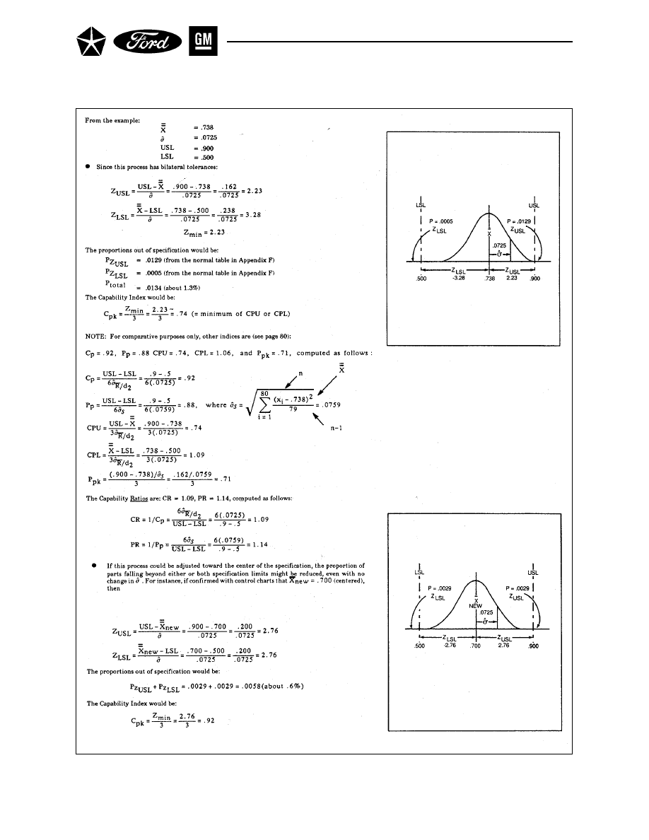
Figure 21. Calculating the Process Capability

- 58 -

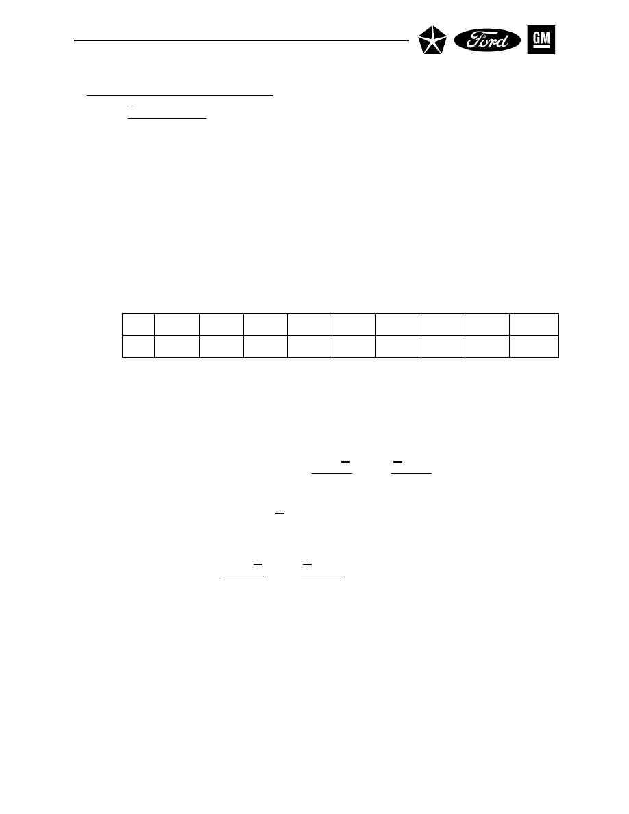
II. CONTROL CHARTS FOR VARIABLES

Section 1. X and R Charts (Cont.) – Interpret for Process Capability

NOTE:

Any capability analysis technique, no matter how precise it appears, can give only
approximate results. This happens because (1) there is always some sampling variation,
(2) no process is ever “fully” in statistical control, and (3) no actual output “exactly”
follows the normal distribution (or any other simple distribution). Final results should
always be used with caution and interpreted conservatively.

D.1.

Calculate the Process Standard Deviation

Since the within-subgroup process variability is reflected in the subgroup ranges, the estimate of
the process standard deviation σ

(“sigma hat”) can be based on the average range ( R

–

). Calculate:

= R

–

= σ

–

/d2

where R

–

is the average of the subgroup ranges (for periods with the ranges in control) and d2 is a

constant varying by sample size, as shown in the partial table below, taken from Appendix E:

This estimate of the process standard deviation (σ

–

/d2

) can be used in evaluating the process

capability, as long as both the ranges and averages are in statistical control.

D.2.

Calculate the Process Capability (See Figure 21.)

Capability can be described in terms of the distance of the process average from the specifica-
tion limits in standard deviation units, Z. Drawing a diagram that shows the distribution
curve, X

–

, σ

–

/d2

, the specification limits and the Z values will be helpful.

•

For a unilateral tolerance, calculate: Z =

USL – X or Z = X – LSL , whichever is appropriate.

–

/d2

–

/d2

where SL = specification limit, X = measured process average, and σ

–

/d2

= estimated process

standard deviation.

•

For bilateral tolerances, calculate:

USL

USL – X or Z = X – LSL

–

/d2

–

/d2

min

= Minimum of Z

USL

or Z

LSL

where USL, LSL = upper and lower specification limits; a negative value of Z indicates the
process average is out of specification.

Z values can be used with a table of the standard normal distribution (Appendix F) to estimate
the proportion of output that will be beyond any specification (an approximate value, assuming
that the process is in statistical control and is normally distributed).

•

For a unilateral tolerance, locate the value of Z along the edges of the table in Appendix C. The
units and tenths digits are along the left edge, and the hundredths digit is along the top. The
number found where this row and column intersect is p

, the proportion out of specification. For

instance, for Z = 1.56, the intersection of the 1.5 row and x.x6 column gives p

= .0594, or

about 6%.

1.13

1.69

2.06

2.33

2.53

2.70

2.85

2.97

3.08

- 59 -

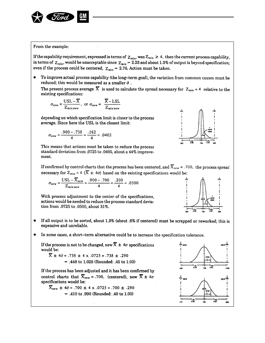
Figure 22. Evaluating the Process Capability

- 60 -

II. CONTROL CHARTS FOR VARIABLES

Section 1. X and R Charts (Cont.) – Interpret for Process Capability

•

For a bilateral tolerance, calculate the proportions beyond upper and lower specification
limits separately. For example, if Z

USL

= 2.21 and Z

LSL

= -2.85, the total beyond specifica-

tion is Pz

USL

+ Pz

LSL

= .0136 + .0022 = .0158, or about 1.6%.

The value Z

min

an also be converted to a Capability Index, C

, defined as:

Cpk =

min

= Minimum of CPU

(

i.e.,

USL – X

)

or CPL

(

i.e.,

X – LSL

)

3σ

–

/d2

3σ

–

/d2

where USL and LSL are the upper and lower engineering specifications, X is the process

average, and σ

is the process standard deviation, computed using R

–

A process with Z

min

= 3 would have a Capability Index C

= 1.00. If Z

min

= 4, the process would

have C

= 1.33.

D.3.

Evaluate the Process Capability (See Figure 22.)

At this point, the process has been brought into statistical control and its capability index has
been described in terms of Z

min

or C

. The next step is to evaluate the process capability in

terms of meeting customer requirements.

The fundamental goal is never-ending improvement in process performance. In the near-term,
however, priorities must be set as to which processes should receive attention first. This is
essentially an economic decision. The circumstances vary from case to case, depending on the
nature of the particular process in question and the performance of other processes which
might also be candidates for immediate improvement action.

While each decision could be resolved individually, it is often helpful to use broader guidelines
to set priorities and promote consistency of improvement efforts. For instance, certain proce-
dures refer to across-the-board capability index requirements of Z

min

≥ 3, or C

≥ 1.00, and

further specify capability index requirements of Z

min

≥ 4, or C

≥ 1. 33 for new processes

affecting selected significant product characteristics. These requirements are intended to as-
sure a minimum performance level that is consistent among characteristics, products, and
manufacturing sources. However, please refer to Section 5 of this chapter for more under-
standing of the interpretation of the C

and other process measures relative to establishing

measure requirements.

Whether in response to a capability index criterion that has not been met, or to the continuing
need for improvement of cost and quality performance beyond minimum capability index re-
quirements, the action required is the same:

•

Improve the process performance by reducing the variation that comes from common causes,
or shift the process average closer to the target. This generally means taking manage-
ment action to improve the system.

In those cases where more immediate action is necessary to meet short-term needs, two stop-
gaps may be available:

•

Sort output and scrap or rework as necessary (thus adding cost and tolerating waste).

•

Alter the specifications for consistency with the process performance (this improves nei-
ther the process nor customer satisfaction).

These are both clearly inferior to process improvement.

- 61 -

IMPROVE THE PROCESS CAPABILITY

To improve the capability (and thus, the performance) of the
process, concentrate on reducing the common causes.
These will usually require management action on the system
to correct.

CHART AND ANALYZE THE REVISED PROCESS

Conform the effectiveness of system changes by continued
monitoring of the control chart.

- 62 -

II. CONTROL CHARTS FOR VARIABLES

Section 1. X and R Charts (Cont.) – Interpret for Process Capability

D.4.

Improve the Process Capability

To improve process capability, there must be increased attention on reducing common causes.
Actions must be directed toward the system, namely, the underlying process factors which ac-
count for the process variability, such as machine performance, consistency of input materials,
the basic methods by which the process operates, training methods, or the working environment.
As a general rule, these system-related causes for unacceptable process capability may be beyond
the abilities of operators or their local supervision to correct. Instead, they may require manage-
ment intervention to make basic changes, allocate resources, and provide the coordination needed
to improve the overall process performance. Attempts to correct the system with short-range
local actions will be unsuccessful.

Discussions of techniques for analysis of system variability are included in several of the refer-
ences listed in Appendix H. Basic problem-solving techniques such as Pareto analysis and cause-
and-effect analysis can be helpful (see Appendix H, Reference 11). However, use of more ad-
vanced methods of process analysis including statistical techniques such as designed experi-
ments may be necessary to achieve significant reductions. See Appendix H, References 7-13 for
introductions to some of these more advanced methods.

D.5.

Chart and Analyze the Revised Process

When systematic process actions have been taken, their effects should be apparent in the control
charts. The charts become a way of verifying the effectiveness of the action.

As the process change is implemented, the control chart should be monitored carefully. This
change period can be disruptive to operations, potentially causing new control problems that
could obscure the effect of the system change.

After any instabilities of the change period have been resolved, the new process capability should
be assessed and used as the basis of new control limits for future operations. Frequently, 25
subgroups of data after the change are sufficient to establish the new control limits.

- 63 -

Figure 23. Data Collection

DATA COLLECTION

PRIMER THICKNESS (MILS)

SAMPLE-SIZE – 10 CONSECUTIVE PIECES TWICE PER DAY

1-11

1-12

1-13

1-14

1-15

1-18

1-19

1.30

1.01

1.22

1.08

.98

1.12

.92

1.04

1.08

1.20

1.25

1.24

1.13

1.08

1.10

1.05

1.12

1.30

1.10

1.14

.92

1.13

.91

1.34

1.16

1.31

1.20

1.15

.93

1.11

1.31

1.01

1.13

1.18

1.14

1.19

.96

1.40

1.12

1.25

.97

1.08

1.28

1.12

1.20

1.02

1.12

1.20

1.16

1.04

1.26

1.22

1.18

1.05

1.25

1.15

1.00

1.08

1.11

.93

1.00

1.02

1.03

.93

1.13

1.12

1.15

.95

1.12

1.27

.95

1.10

.93

1.17

1.02

1.04

1.25

1.08

1.15

1.07

1.17

1.10

.95

1.15

1.02

1.24

1.05

.94

1.20

1.29

1.08

1.04

.98

1.16

.90

1.11

1.14

1.35

1.25

.98

1.34

1.05

1.24

1.42

1.02

1.28

1.05

1.37

1.04

1.12

1.28

1.12

1.05

1.34

1.12

1.10

1.05

1.12

1.00

.98

1.08

1.10

1.31

1.26

1.10

1.12

1.05

1.06

1.03

1.00

1.18

1.10

1.26

1.15

1.07

1.10

1.14

1.18

1.11

1.10

1.11

1.06

1.15

1.10

1.19

1.14

1.13

.136

.098

1.06

.120

.121

.115

.136

.101

.086

.079

.170

.125

.070

.107

1-20

1-21

1-22

1.08

1.14

1.06

1.14

1.07

1.13

1.26

1.02

1.12

1.22

1.05

.90

1.13

1.14

.98

1.18

.97

1.12

.94

1.12

1.27

1.05

1.04

1.30

1.20

1.17

1.16

1.40

1.15

1.08

1.02

1.26

1.02

1.12

1.07

.94

1.19

1.15

1.02

1.15

1.02

1.12

1.03

1.07

1.14

1.01

1.22

1.15

1.02

1.07

1.30

1.18

1.36

1.09

1.36

1.00

1.14

1.12

1.08

1.18

1.06

1.13

.111

.137

.074

.099

.059

.141

- 64 -

II. CONTROL CHARTS FOR VARIABLES

Section 2

AVERAGE AND STANDARD DEVIATION CHARTS ( X

–

AND s)

–

and s charts, like X

–

and R charts, are developed from measured process output data, and are always used

as a pair. Range charts were developed as measures of process variation because the range is easy to
calculate and is relatively efficient for small subgroup sample sizes (especially below 9). The sample stan-
dard deviation, s, is a more efficient indicator of process variability, especially with larger sample sizes.
However, it is more complex to calculate, and it is less sensitive in detecting special causes of variation that
cause only a single value in a subgroup to be unusual. Typically, s charts are used instead of R charts when
one or more of the following exists:

•

The data are recorded and/or charted by computer on a real-time basis, so a calculation routine for s is
easily integrated.

•

Ready availability of a pocket calculator makes computation of s simple on a routine basis.

•

Large subgroup sample sizes are used, and the more efficient measure of variation is appropriate.

The details of instructions for X

–

and s charts are very similar to those for X

–

and R charts; exceptions are

noted below:

A. GATHER DATA

(See Section 1, Part A of this chapter, exceptions are noted below)

• If raw data are voluminous, they are often recorded on a separate data sheet (see Figure 23),

with only each subgroup’s X

–

and s appearing on the chart itself.

• Calculate each subgroup’s sample standard deviation using one of the following equivalent

formulas:

s =

√

– X

–

)

n – 1

s =

√

– X

–

√

+ X

+ ... + X

– nX

–

n – 1

where X

, X

–

, and n represent the subgroup’s individual values, average, and sample size.

NOTE:

Do not round off X

–

values if computing longhand.

•

The scale spacing for the s chart should be the same as for its corresponding X

–

chart.

- 65 -

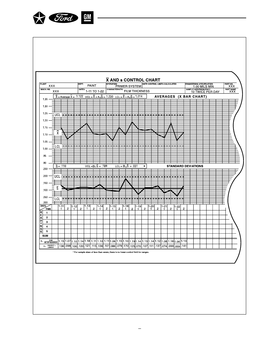
Figure 24. X and s Chart

- 66 -

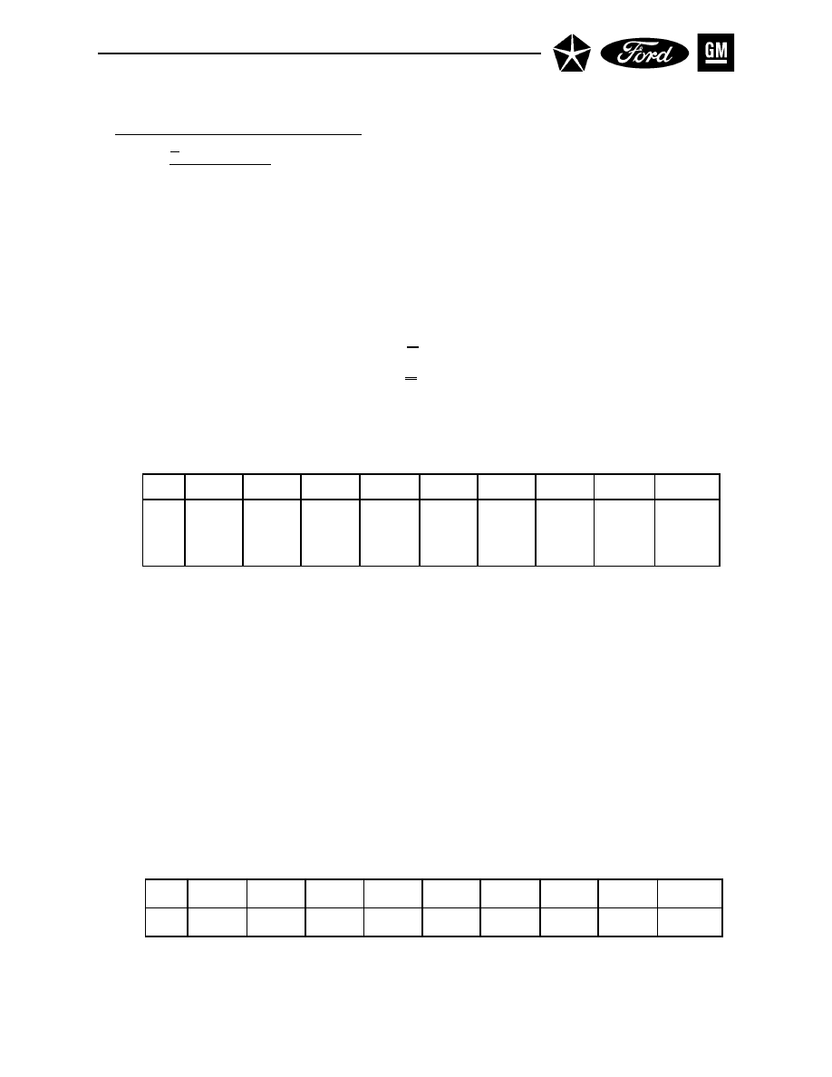
II. CONTROL CHARTS FOR VARIABLES

Section 2. X and s Charts (Cont.)

B. CALCULATE CONTROL LIMITS (See Figure 24.)

(See Section 1, Part B of this chapter, exceptions are noted below)

• Calculate the upper and lower control limits for standard deviations and averages (UCL

, LCL

UCL

–

, LCL

–

UCL

= B

s–

LCL

= B

s–

UCL

–

= X + A

s–

LCL

–

= X – A

s–

where s is the average of the individual subgroup sample standard deviations, and B4, B3, and A3
are constants varying by sample size, with values for sample sizes 2 to 10 shown in the following
partial table, taken from Appendix E.

There is no lower control limit for standard deviations for sample sizes below 6.

C. INTERPRET FOR PROCESS CONTROL

(See Section 1, Part C of this chapter.)

D. INTERPRET FOR PROCESS CAPABILITY

(See Section 1, Part D of this chapter; exceptions are noted below)

• Estimate the process standard deviation:

= s–/c

= σ

s–

where s is the average of the sample standard deviations (for periods with the standard deviation
under control) and c4 is a constant varying by sample size, with values for sample sizes from 2 to
10 shown in the following partial table, taken from Appendix E:

• If the process has a normal distribution, this estimate of a can be used directly in assessing process

capability, as long as both averages and standard deviations are in statistical control.

.798

.886

.921

.940

.952

.959

.965

.969

.973

3.27

2.57

2.27

2.09

1.97

1.88

1.82

1.76

1.72

.03

.12

.19

.24

.28

2.66

1.95

1.63

1.43

1.29

1.18

1.10

1.03

.98

- 67 -

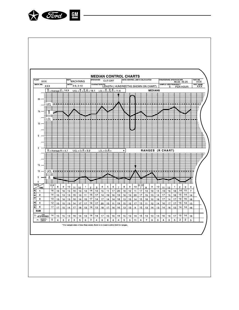
Figure 25. Median Control Chart

- 68 -

II. CONTROL CHARTS FOR VARIABLES

Section 3

MEDIAN CHARTS (

AND R)

Median charts (see Figure 25) are alternatives to X

–

and R charts for control of processes with measured

data; despite the fact that medians may not be as statistically desirable as averages, median charts yield
similar conclusions and have some advantages:

• Median charts are easy to use, and do not require many calculations. This can increase shop-floor

acceptance of the control chart approach.

• Since individual values (as well as medians) are plotted, the median chart shows the spread of

process output and gives an ongoing picture of the process variation.

• Since a single chart shows both the median and spread, it can be used to compare the output of

several processes, or of the same process at successive stages.

Instructions for median charts are similar to X

–

and R charts; exceptions are noted:

GATHER DATA

(See Section 1, Part A of this chapter; exceptions are noted below)

• Typically, median charts are used with subgroup sample sizes of 10 or less; odd sample sizes are

most convenient. If using even size subgroups, the median is the average of the middle two units.

• Only a single graph may be plotted; set the scale to include the larger of (a) the product specifica-

tion tolerance plus an allowance for out-of-specification readings, or (b) 1-1/2 to 2 times the differ-
ence between the highest and lowest individual measurement. The graph scales should agree with
the gage.

• Plot the individual measurements for each subgroup in a vertical line. Circle the median of each

subgroup (the middle value; if the sample size is an even number, the median will be midway
between the inner points). To aid in interpreting trends, connect the subgroup medians by a line.

• Enter each subgroup’s median ( X ) and range (R) in the data table. It is recommended to also plot

the range chart to observe trends or runs in the range.

B. CALCULATE CONTROL LIMITS

(See Section 1, Part B of this chapter; exceptions are noted below)

• Find the average of the subgroup medians and draw this as the central line on the chart; record

this as X

• Find the average of the ranges; record this as R

–

• Calculate the upper and lower control limits for ranges and medians ( UCL

, LCL

, UCL

, LCL

UCL

= D

–

LCL

= D

–

UCL

= X + A

–

LCL

= X + A

–

- 69 -

– ~

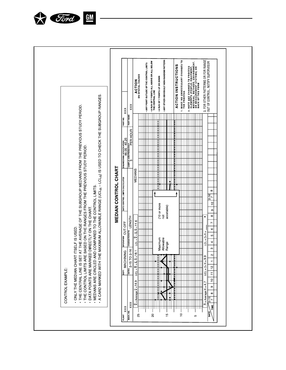
Figure 26. Median Control Chart – Interpretation

- 70 -

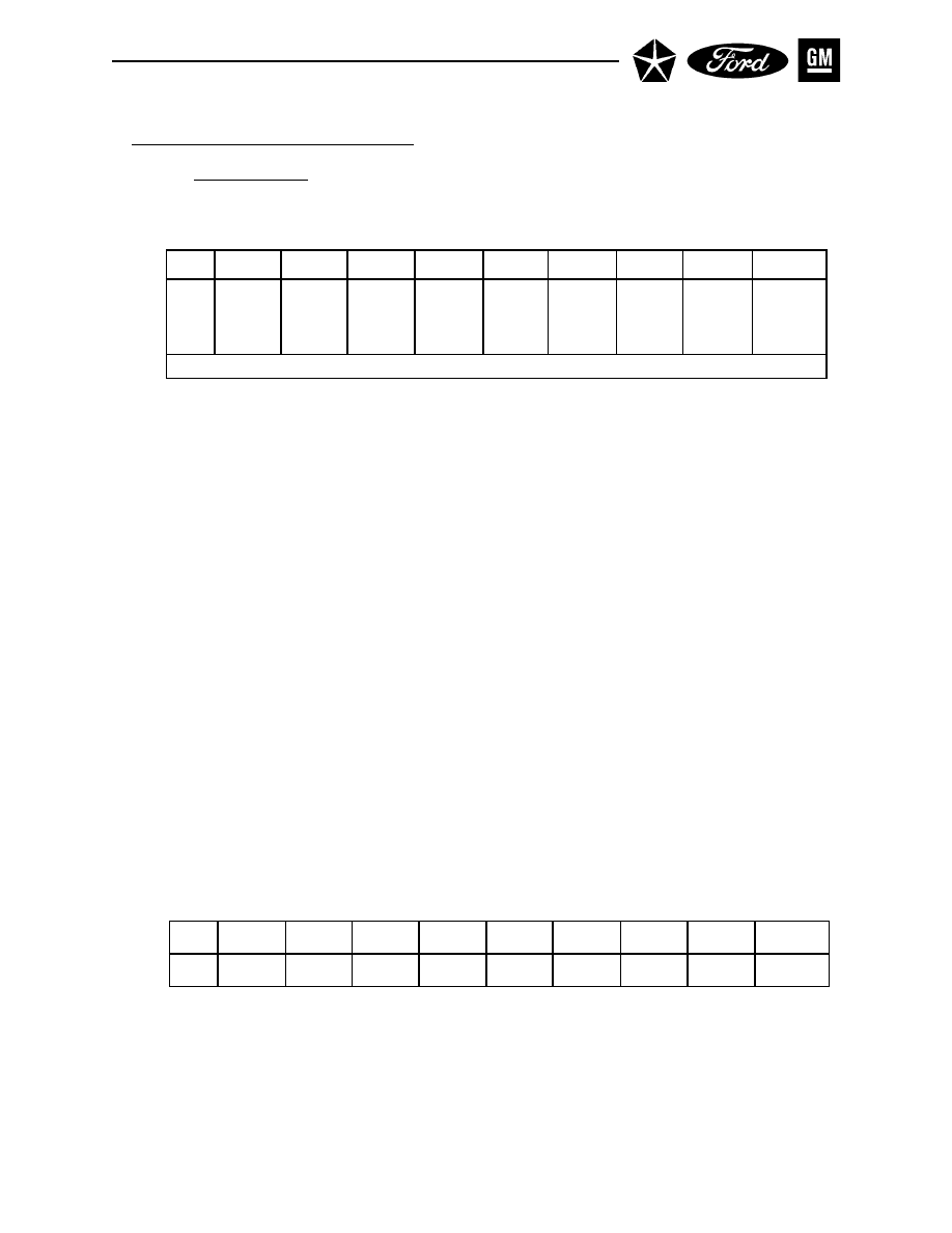
II. CONTROL CHARTS FOR VARIABLES

Section 3. Median Charts (Cont.)

where D

, D3, and A

are constants varying by sample size, with values for sample sizes 2 to 10 shown in

the following table, taken from Appendix E.

•

Plot the control limits for medians on the chart.

C. INTERPRET FOR PROCESS CONTROL

(See Section 1, Part C of this chapter; exceptions are noted below)

• Compare the UCL

and LCL

with each calculated range. Alternatively, mark the edge of an index

card with the points corresponding to the control limits for ranges, and compare these marks with
the distance between the highest and lowest value in each subgroup. Draw a narrow vertical box
to enclose any subgroup with excessive range.

• Mark any subgroup median that is beyond the median control limits, and note the spread of

median within the control limits (2/3 of points within middle third of limits) or the existence of
patterns or trends (see Figure 26).

• Take appropriate process action for special–causes affecting the ranges or medians.

D. INTERPRET FOR PROCESS CAPABILITY

(See Section 1, Part D of this chapter; exceptions are noted below)

• Estimate the process standard deviation:

= R

–

where R

–

is the average of the sample ranges (for periods with the range under control) and d

is a

constant varying by sample size, with values for sample sizes from 2 to 10 shown in the following
table, taken from Appendix E.

• If the process has a normal distribution, this estimate of σ can be used directly in assessing process

capability, as long as the medians and ranges are in statistical control.

1.13

1.69

2.06

2.33

2.53

2.70

2.85

2.97

3.08

3.27

2.57

2.28

2.11

2.00

1.92

1.86

1.82

1.78

.08

.14

.18

.22

1.88

1.19

.80

.69

.55

.51

.43

.41

.36

* There is no lower control limit for ranges for sample sizes below 7.

- 71 -

– ~

II. CONTROL CHARTS FOR VARIABLES

Section 3. Median Charts (Cont.)

E. ALTERNATE APPROACH TO MEDIAN CHART

For ongoing process control where control limits are based on prior data, the charting process can be
simplified as follows:

• A single chart is used, with scales set at the same increments as the gage being used (at least 20

increments between product specifications), and with the central line and control limits for medi-
ans already entered.

• A card (possibly plastic) is provided, marked with the control limits for ranges. This assumes the

special causes affecting the ranges generate out of control points and not trends.

• The operator marks the chart with each individual reading, but the numerical values do not need

to be recorded.

• For each subgroup, the operator compares the range card to the subgroup’s highest and lowest

marks; any subgroup having a range beyond the limits on the card is enclosed in a narrow vertical
box.

• The operator counts to the median of each subgroup and circles it; any median beyond either

control limit is marked.

• For ranges or medians beyond control limits, the operator takes appropriate actions to adjust or

correct the process, or to notify supervisory or support people.

- 72 -

- 73 -

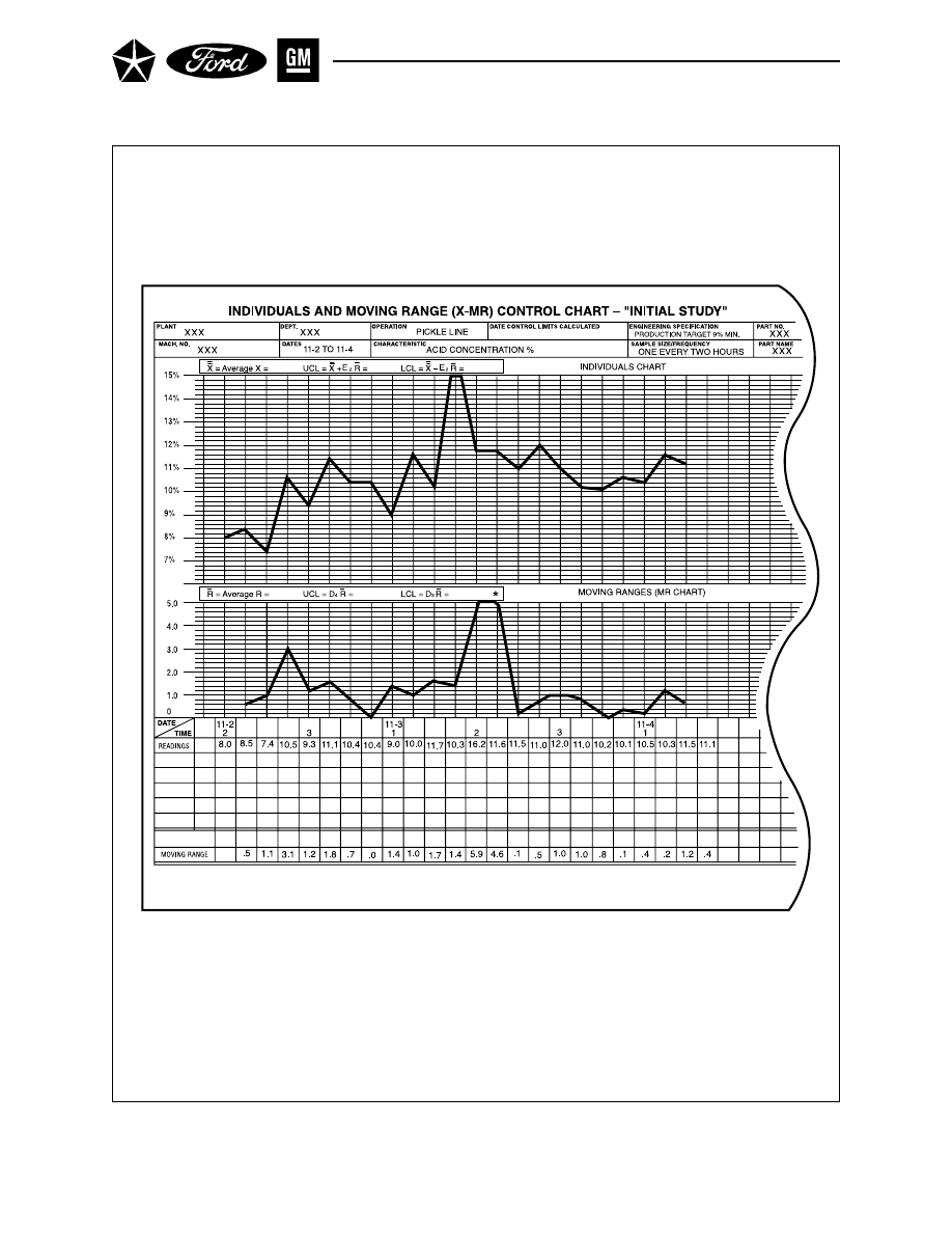
Figure 27. Individuals and Moving Range Chart

- 74 -

II. CONTROL CHARTS FOR VARIABLES

Section 4

CHARTS FOR INDIVIDUALS AND MOVING RANGE (X–MR)

In some cases, it is necessary for process control to be based on individual readings, rather than subgroups.
In such cases, the within subgroup variation is effectively zero. This would typically occur when the mea-
surements are expensive (e.g., a destructive test), or when the output at any point in time is relatively
homogenous (e.g., the pH of a chemical solution). In these cases, control charts for individuals can be
constructed as described below. Four cautions should be noted, however:

•

Charts for individuals are not as sensitive in detecting process changes as X

–

and R charts.

•

Care must be taken in interpretation of charts for individuals if the process distribution is not sym-
metrical.

•

Charts for individuals do not isolate the piece-to-piece repeatability of the process. In many applica-
tions, therefore, it may be better to use a conventional X

–

and R chart with small subgroup sample sizes

(2 to 4) even if this requires a longer period between subgroups.

•

Since there is only one individual item per subgroup, values of X and σ

can have substantial variabil-

ity (even if the process is stable) until the number of subgroups is 100 or more.

The details of instructions for charts for individuals are somewhat similar to those for X

–

and R charts;

exceptions are noted below:

A. GATHER DATA (See Figure 27.)

(See Section 1, Part A of this chapter; exceptions are noted below)

• Individual readings (X) are recorded from left to right on the data chart.

• Calculate the moving range (MR) between individuals. It is generally best to record the difference

between each successive pair of readings (e.g., difference between the first and second reading, the
second and third, etc.). There will be one less such moving range than there are individual read-
ings (25 readings give 24 moving ranges). In rare cases, the moving range can be based on a larger
moving group (e.g., threes or fours), or on a fixed subgroup (e.g., all the readings taken on a single
shift). Note that even though the measurements are sampled individually, it is the number of
readings grouped to form the moving range (e.g., 2, 3 or 4) which determines the nominal sample
size n. This must be considered when consulting factor tables.

• Select scales for the chart for individuals (X) equal to the larger of (a) the product specification

tolerance plus an allowance for out-of-specification readings, or (b) 1-1/2 to 2 times the difference
between the highest and lowest individual readings. The scale spacing for the chart for moving
ranges (MR) should be the same as that of the X chart.

B. CALCULATE CONTROL LIMITS (See Figure 28.)

(See paragraph B, Section 1 of this chapter; exceptions are noted below)

• Calculate and plot the process average (the sum of individual readings, divided by the number of

readings; by convention, labeled X; see the Glossary in Appendix G), and calculate the average
range ( X

–

); note that for a moving range of sample size two there is one less moving range value

(MR) than the number of individual readings (X).

- 75 -

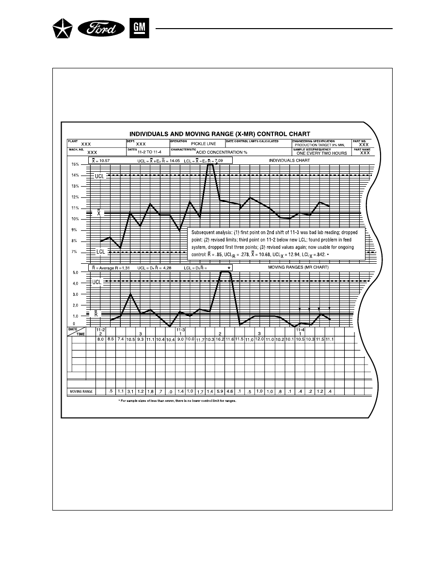
Figure 28. Interpretation of Individuals and Moving Range Chart

- 76 -

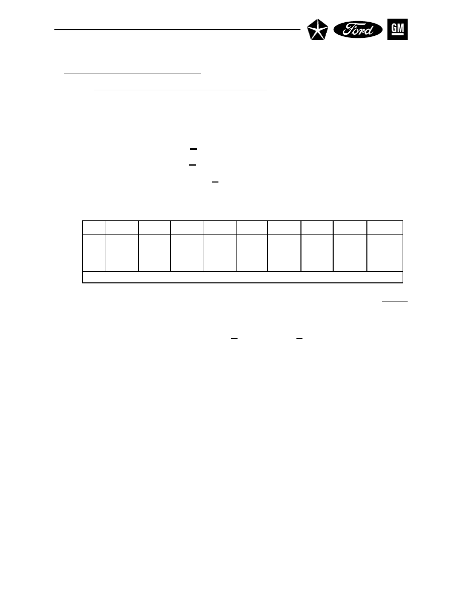
II. CONTROL CHARTS FOR VARIABLES

Section 4. Individuals and Moving Range (X–MR) Charts (Cont.) – Calculate Control Limits

• Calculate the control limits:

UCL

= D

–

LCL

= D

–

UCL

= X + E

–

LCL

= X – E

–

where R

–

is the average moving range, X is the process average, and D

, D

and E

are constants

that vary according to the sample size, n, used in grouping the moving ranges, as shown in the
following partial table, taken from Appendix E.

NOTE:

An alternate approach to calculating control limits when R

–

is greater than the median

range, R (as is generally the case), is to use the median range for 2 piece moving ranges
and compute control limits as follows (see Appendix H, Reference 23):

UCL

= 3.865 R; LCL

= 0

UCL

= X + 3.14 R; LCL

= X – 3.14 R

C. INTERPRET FOR PROCESS CONTROL (See Figure 28.)

(See Section 1, Part C of this chapter; exceptions are noted below)

• Review the moving range chart for points beyond the control limits as signs of the existence of

special causes. Note that successive moving ranges are correlated, since they have at least one
point in common; because of this, care must be taken when interpreting trends. Advice from a
statistician might be required for trend interpretations.

• The chart for individuals can be analyzed for points beyond the control limits, spread of points

within the control limits, and trends or patterns. Note here, though, that if the process distribution
is not symmetrical, the rules shown previously for X

–

charts may give signals of special causes

when none exist.

D. INTERPRET FOR PROCESS CAPABILITY (See Figure 28.)

(See Section 1, Part D of this chapter; exceptions are noted below)

• As with X

–

and R charts, the process standard deviation can be estimated by:

= R

–

= σ

R/d

where R

–

is the average of the moving ranges and d

is a constant varying by the sample size, n,

used in grouping the moving ranges as shown in the partial table below, taken from Appen

dix E.

3.27

2.57

2.28

2.11

2.00

1.92

1.86

1.82

1.78

.08

.14

.18

.22

2.66

1.77

1.46

1.29

1.18

1.11

1.05

1.01

.98

* There is no lower control limit for ranges for sample sizes below 7.

- 77 -

II. CONTROL CHARTS FOR VARIABLES

Section 4. Individuals Chart (Cont.) – Interpret for Process Capability

•

If the process has a normal distribution, this estimate of

can be used directly in assessing

process capability, as long as the process is in statistical control.

1.13

1.69

2.06

2.33

2.53

2.70

2.85

2.97

3.08

- 78 -

II. CONTROL CHARTS FOR VARIABLES

Section 5

UNDERSTANDING PROCESS CAPABILITY AND PROCESS

PERFORMANCE FOR VARIABLES DATA

The output of a statistically stable (in control) manufacturing process can be described by its distribution.
Characteristics of the distribution are used to evaluate the process. For instance, a characteristic of fre-
quent interest is the center of the distribution. If the distribution is not properly located, the manufactur-
ing process may produce parts that are not close enough to a desired target value. In such cases, some
parts may even be out-of-specification. A process with such a distribution may then be assessed as inca-
pable of meeting the customer’s needs. Similar problems may occur if the distribution has too much spread,
regardless of where the distribution is located. Because the characteristics of the distribution are not
known exactly, data must be gathered to estimate them.

This section addresses some of the techniques used for estimating how certain of the characteristics of the
distribution relate to specifications. The underlying pre-condition that the process from which the data
come exhibits statistical stability should be reemphasized here. A discussion of process variation and the
associated capability indices has little value for unpredictable processes. Be aware, however, that reason-
able approaches for assessing process capability have been developed for processes exhibiting systematic
special causes of process variation, such as tool wear (see Appendix H, Reference 17). In addition, it is
generally assumed that the individual readings from the subject processes have a distribution that is
approximately normal. After defining process capability and related terms, this section will define and
discuss only the more popular indices and ratios, as follows:

Indices of process variation only, relative to specifications: C

, and P

Indices of process variation and centering combined, relative to specifications: CPU, CPL, C

, and P

Ratios of process variation only, relative to specifications: CR and PR

NOTE:

Although other indices are not discussed in this manual, Appendix D and Appendix H,
Reference 16 do provide information on one of these, C

, a relatively new index which

has gained some recent attention.

Finally, this section describes the conditions and assumptions associated with these process measures
and concludes with a suggestion as to how these measures might be applied toward enhancing pro-
cess understanding within the framework of continual process improvement.

This manual fully recognizes both the misunderstanding and controversy which surrounds funda-
mental concepts and definitions relative to the issues of process “Control”, “Capability”, and “Perfor-
mance”. It is appropriate to point out here that it is not the purpose of this manual to fully resolve
these issues, but to expose and discuss them to an extent which allows each reader the opportunity to
develop a better understanding of them in order to provide value and knowledge for continual process
improvement.

A. DEFINITION OF PROCESS TERMS

• Inherent Process Variation – That portion of process variation due to common causes only. This

variation can be estimated from control charts by R

–

, among other things (e.g., s

–/c

• Total Process Variation – This is the variation due to both common and special causes. This varia-

tion may be estimated by s, the sample standard deviation, using all of the individual readings

obtained from either a detailed control chart or a process study: i.e., s =

√

i=1

n - 1

- x

–)

= σ

s , where

is an individual reading, X

–

is the average of the individual readings, and n = the total number of

all of the individual reaadings.

- 79 -

II. CONTROL CHARTS FOR VARIABLES

Section 5. Understanding Capability (Cont.) - Definition of Process Measures

• Process Capability — The 6a range of a process’s inherent variation, for statistically stable pro-

cesses only, where a is usually estimated by R

–

(σ

–

/d2

• Process Performance — The 6 a range of a process’s total variation, where a is usually estimated by

s, the sample standard deviation (σ

s).

B. DEFINITION OF PROCESS MEASURES

B.1.

Indices

This is the capability index which is defined as the tolerance width divided by the process
capability, irrespective of process centering. Typically, this is expressed as

Cp =

USL - LSL

6σ

–

/d2

This is the performance index which is defined as the tolerance width divided by the
process performance, irrespective of process centering. Typically, this is expressed as

USL – LSL

(it should tee used only to compare to or with C

and C

and to measure

6σ

and prioritize improvement over time).

CPU: This is the upper capability index and is defined as the upper tolerance spread divided by

the actual upper process spread. Typically, this is expressed as CPU = USL – X .

3σ

–

/d2

CPL: This is the lower capability index and is defined as the lower tolerance spread divided by

the actual lower process spread. Typically, this is expressed as CPL = X – LSL .

3σ

–

/d2

This is the capability index which accounts for process centering and is defined as the
minimum of CPU or CPL. It relates the scaled distance between the process mean and
the closest specification limit to half the total process spread.

This is the performance index which accounts for process centering and is defined as the

minimum Of USL – X or X – LSL (it should be used only to compare to or with C

and

3σ

s 3σ

and to measure and prioritize improvement over time).

B.2.

Ratios

CR:

This is the capability ratio and is simply the reciprocal of C

; i.e., CR =

6σ

–

/d2

USL-LSL

PR:

This is the performance ratio and is simply the reciprocal of P

; i.e., PR =

6σ

USL-LSL

NOTE: Example calculations for all of these measures are shown on page 58.

- 80 -

II. CONTROL CHARTS FOR VARIABLES

Section 5. Understanding Capability (Cont.) - Definition of Process Measures

B.3. Clarification of Sample Standard Deviation - s vs. s

Both s (used in parts A and B of this section) and s (used in X

–

and s charts, page 65) are calculated

using exactly the same formula for sample standard deviation: i.e., s and s =

√

i=1

n - 1

- x

–)

However, the “n” in the formula symbolizes two different types of sample sizes, as follows:

• For s (page 79), n refers to the total number of all of the individual values sampled - for

example, the number of these individual values can come from the total of the number of all
of the subgroup individual values from a control chart (all totaled together), or from a broad
sampling of an overall population.

• For s (page 65), n refers only to the number of individual values within any given subgroup

generally, n is a constant and equal number for each subgroup.

• σ

s estimates the standard deviation of a total process (“population”) using s, while σ

s esti-

mates the standard deviation of a given subgroup of fixed size, using s (see pages 65-67).

C. DESCRIPTION OF CONDITIONS AND ASSUMPTIONS

It is appropriate to point out that process variation and process centering are two separate process
characteristics. Each needs to be understood separately from the other. However, in order to minimize
separate analyses of each, it has become convenient to combine the two characteristics into one index,
such as C

or P

. These indices can be useful for:

• Measuring continual improvement using trends over time.

• Prioritizing the order in which processes will be improved.

The capability index (e.g., C

) is additionally useful for determining whether or not a process is

capable of meeting customer requirements (the original intent of the capability index). It should be
pointed out that this additional use should not be applied to performance indices (see page 80 for
suggested use of performance measures).

For these indices (as well as all of the other process measures described in part B of this section) to be
effectively used, the CONDITIONS and ASSUMPTIONS which surround them must be understood.
If these conditions and assumptions are not met, the measures will have little or no meaning and thus
add no value to understanding the processes from which they were generated. Following are the four
minimum conditions which must be satisfied for all of the capability measures that are described in
Part B of this section:

• The process from which the data come is statistically stable.

• The individual measurements from the process data form an approximately normal distribution.

• The specifications are based on customer requirements.

• There exists a willingness to accept the computed index (or ratio) value as the “true” index (or

ratio) value - i.e., to discount sampling variation’s influence on the computed number (e.g., a com-
puted C

of 1.05 may be from a process whose “true” C

is 1.40, or vice versa, due simply to

sampling variation). Please see Appendix H, References 19, 20, and 21 for more on this subject.

- 81 -

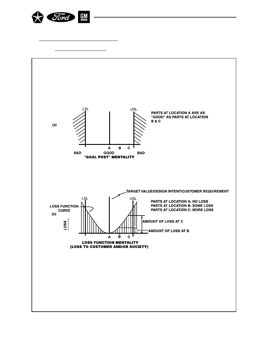
- 82 -

Figure 29. “Goal Post” vs. Loss Function

II. CONTROL CHARTS FOR VARIABLES

Section 5. Understanding Capability (Cont.) - Suggested Use of Process Measures

II. CONTROL CHARTS FOR VARIABLES

Section 5. Understanding Capability (Cont.)

D. SUGGESTED USE OF PROCESS MEASURES

The key to effective use of any process measure continues to be the level of understanding of what the
measure truly represents. Those in the statistical community who generally oppose how C

numbers,

for instance, are being used are quick to point out that few “real world” processes completely satisfy all
of the conditions, assumptions, and parameters within which C

has been developed (see Appendix

H, Reference 14 and Reference 18). Further, it is the position of this manual that, even when all
conditions are met, it is difficult to assess or truly understand a process on the basis of a single index
or ratio number, for reasons discussed in the paragraphs below.

D.1.

The Loss Function Concept

The driving force behind how capability indices (and other process measures) have been used has
been the understandable desire to produce all parts within engineering specifications. The un-
derlying concept serving as the motivation for this desire is the mentality that all parts within
specification, regardless of where they are located or positioned within the specification range,
are “good” (or acceptable), and all parts beyond specifications, regardless of how far beyond speci-
fications they may be, are “bad” (or unacceptable). Quality professionals sometimes refer to this
concept as “Goal Post” mentality (see Figure 29 (a)).

Although this mental model (good/bad) has been extensively used in the past, it is suggested that
a more useful model, i.e., one that is a lot closer to the behavior of the real world, is the one
pictured in Figure 29 (b). This model takes, in general, the form of a parabola and utilizes the
principle that an increasing quadratic (as opposed to linear) loss is incurred by the customer and/
or society the further a particular characteristic gets from the specification target. Implicit in this
concept, referred to as the loss function concept, is the presumption that the design intent (speci-
fication target) is reasonably well aligned with the customer’s requirement.

- 83 -

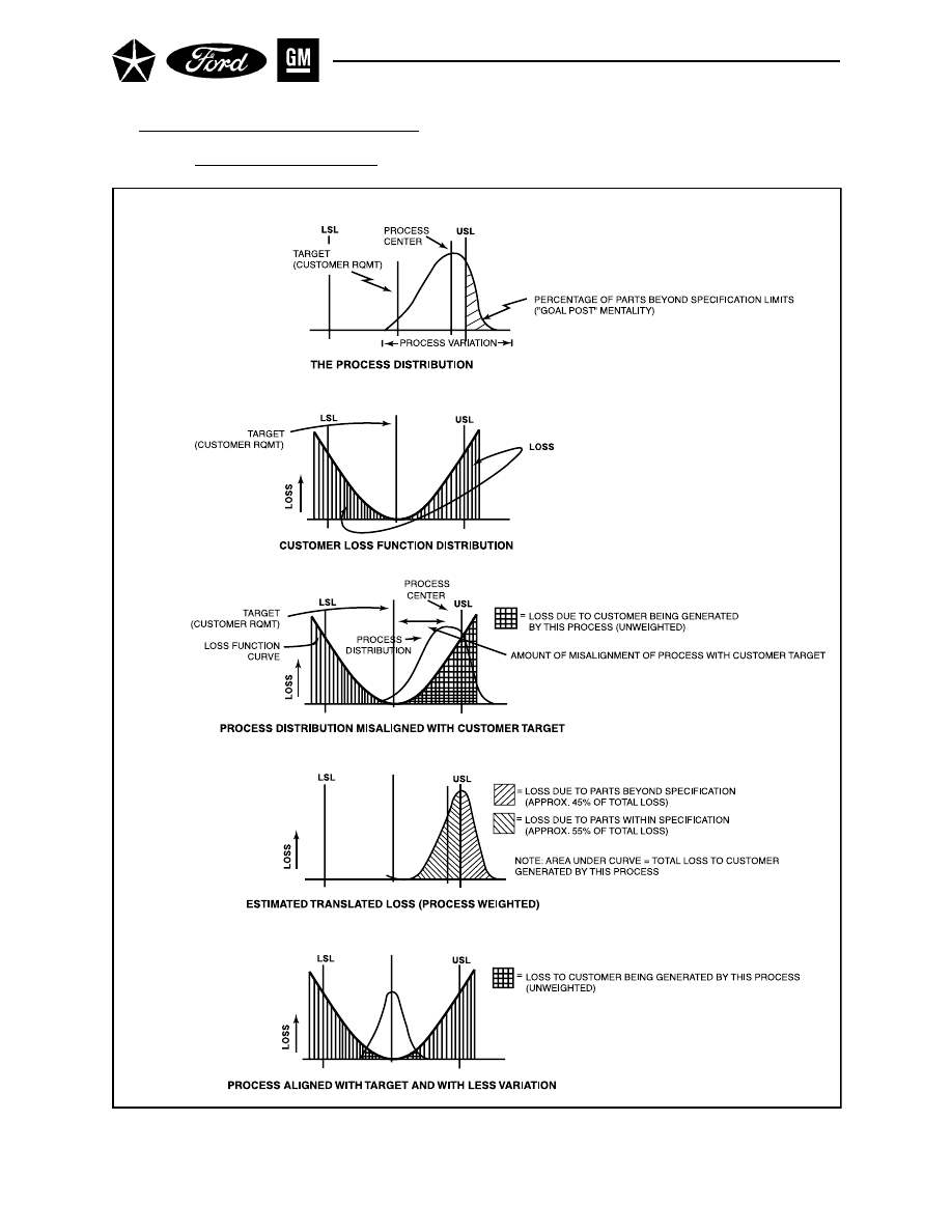
- 84 -

Figure 30. Process Alignment to Requirements

II. CONTROL CHARTS FOR VARIABLES

Section 5. Understanding Capability (Cont.) - Suggested Use of Process Measures

(e)

(d)

(c)

(b)

(a)

II. CONTROL CHARTS FOR VARIABLES

Section 5. Understanding Capability (Cont.) Suggested Use of Process Measures

D.2.

Alignment of Process to Customer Requirements

In Section 2 of Chapter I, a process was depicted graphically (see Figure 1, page 6). An output
characteristic of such a process can also be expressed graphically in terms of a distribution of its
variation. This distribution might be referred to as the process distribution (see Figure 30 (a)).

A loss function such as the one depicted in Figure 30 (b) can be established for the process char-
acteristic whose distribution is indicated in Figure 30 (a). Further, assuming little or no variation
in the customer requirement (specification target), by superimposing the process distribution
onto the customer requirement loss function curve (Figure 30 (c)), two observations can be made:

• In order to minimize customer losses, it is desirable to align the process (process center) with

the customer requirement (specification target).

• It is additionally beneficial to the customer if variation around the target value is continually

reduced (see (Figure 30 (e)).

This analysis is sometimes called aligning the “Voice of the Process” with the “Voice of the Cus-
tomer” (see Appendix H, Reference 22, for more detail). It should be noted that although no
variation is assumed in the “Voice of the Customer” for this example, the “Voice of the Customer”
(specification target) does vary in the real world and this further complicates achieving true
customer satisfaction with a given process.

Finally, when an estimated translated loss is generated by considering the actual distribution of
parts being produced by this process, in conjunction with the loss being generated by this pro-
cess, it can be shown that, in this case, approximately only 45% of the total loss to the customer
is being accounted for by the parts beyond specification, while the remaining loss is coming from
parts within specification but not at the target (Figure 30 (d)). This strongly suggests that the
“Goal Post” mentality, or computing percentage of “Bad” parts (parts beyond specifications), in
and of itself, does not provide a proper appreciation for understanding the effect the process is
actually having on the customer.

- 85 -

II. CONTROL CHARTS FOR VARIABLES

Section 5. Understanding Capability (Cont.) - Suggested Use of Process Measures

D.3.

Applications of Process Measures

For reasons discussed in the foregoing paragraphs, and assuming the conditions listed in part C
of this section have been met, the following is suggested relative to using process measures for
enhanced understanding and effective continual improvement of processes:

• No single index or ratio should be used to describe a process; further,

• Two or more indices or ratios should be viewed collectively-At a minimum, the combination of

and C

, P

and P

, CR and C

, or PR and P

, for example, should be used; and

• It is strongly recommended that graphical analyses be used in conjunction with the process

measures. Examples of such analyses include control charts, plots of estimated process distri-
butions, loss function analysis graphs such as those shown in Figure 30, etc. Additionally,
particularly for unstable processes, it might be helpful to also graph or plot inherent process
variation versus total process variation and/or σ

–

/d2

versus σ

s to gain an appreciation for a

rough perception of the gap between the process “capability” and “performance” and to track
improvement. Generally, the size of this gap is a measure of the degree to which the process is
out of control, even though in unstable processes, depending on the degree of instability, there
is respectively more variability and uncertainty in the process estimates (σ

–

/d2

and σ

s) than

for stable processes. These types of graphical analyses should be done for better process un-
derstanding even if process measures (i.e., C

/ C

, etc.) are not computed and/or used.

• For continual process improvement, process measures should be used with the mindset of

continually attempting to match the “Voice of the Process” to the “Voice of the Customer”, with
minimal loss to the customer.

A final precaution is that all capability assessments should be confined to a single process char-
acteristic. It is never appropriate to combine or average the capability results for several pro-
cesses into one index.

Hopefully, the application of process measures within this total framework will provide some of
the information necessary for achieving true process improvement at a competitive rate.

- 86 -

- 87 -

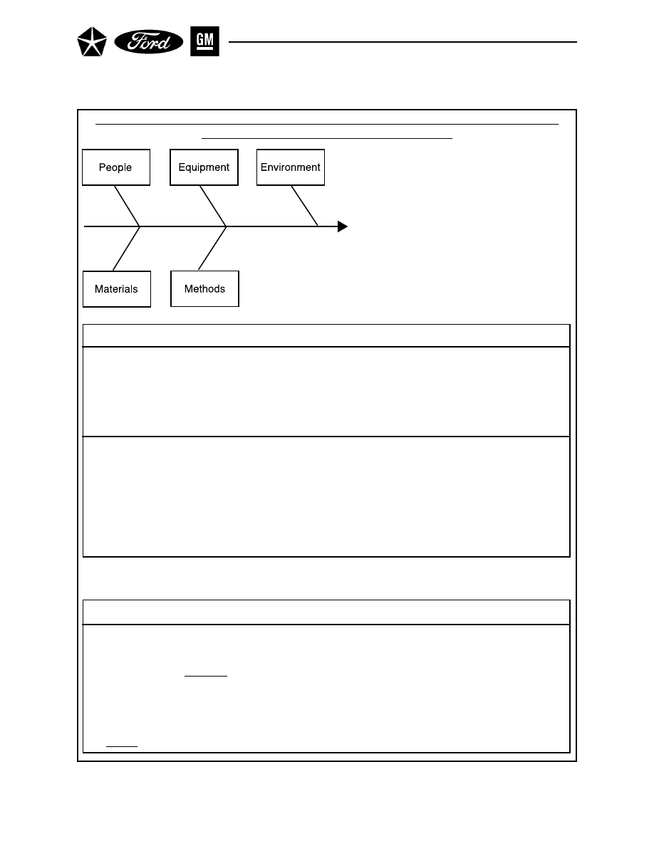
- 88 -

Figure 31. Atrribute Data

Results from Comparing the Process Outcome to an Acceptance Specification and

Deciding if it Conforms of Does Not Conform

• Vehicle does not leak/leaks
• Lamp lights/does not light
• Hole diameter undersized or oversized

(go/no-go gage)

• Shipment to dealer correct or incorrect

• Bubbles in a windshield
• paint imperfections on door
• Errors on an invoice

• p Chart for Proportion

of Units Nonconforming

• np Chart for Number of

Units Nonconforming

• c Chart for Number of

Nonconformities per
Inspection Unit

• u Chart for Number of

Nonconformities per
Inspection Unit

Outcome Examples

Control Charts

The conformance criteria must be clearly defined and the procedures for deciding if
these criteria are met must produce consistent results over time.

• Surface Should be free from flaws

• Surface should conform to master

standard in color texture, brightness
and imperfections

• Any material applied to mirror back to

prevent scattering shall not cause
visible staining of mirror backing.

• What is a flaw?

- Do inspectors agree?
- How measured?

• Conform to what degree?

• How measured?
• Visible to whom?

• Under what conditions

Outcome Examples

Control Charts

Outcome is Classified

Conforms:

“ACCEPT”

Does Not Conform:

“REJECT”

Chapter III

CONTROL CHARTS FOR ATTRIBUTES

Although control charts are most often thought of in terms of variables (as shown in Chapter II), versions
have also been developed for attributes. (See Figure 31.) Attribute data have only two values (conforming/
nonconforming, pass/fail, go/no-go, present/absent) but they can be counted for recording and analysis.*
Examples include the presence of a required label, the continuity of an electrical circuit, or errors in a
typed document. Other examples are of characteristics that are measurable, but where the results are
recorded in a simple yes/no fashion, such as the conformance of a shaft diameter when measured on a go/
no-go gage, the acceptability of door margins to a visual or gage check, or on-time delivery performance.
Control charts for attributes are important for several reasons:

•

Attribute data situations exist in any technical or administrative process, so attribute analysis tech-
niques are useful in many applications. The most significant difficulty is to develop precise operational
definitions of what is nonconforming.

•

Attribute data are already available in many situations-wherever there are existing inspections, writeups
for repair, sorts of rejected material, etc. In these cases, no additional data collection expense is in-
volved, just the effort of converting the data to control chart form.

•

Where new data must be collected, attribute information is generally quick and inexpensive to obtain,
and with simple gaging (e.g., a go/no-go gage) it often does not require specialized collection skills.

•

Much data gathered for management summary reporting is in attribute form and can benefit from
control chart analysis. Examples include department first-run OK performance, scrap rates, quality
audits and material rejections. Because of the ability to distinguish variation from special and com-
mon causes, control chart analysis can be valuable in interpreting these management reports.

•

When introducing control charts into an organization, it is important to prioritize problem areas and
use charts where they are most needed. Problem signals can come from the cost control system, user
complaints, internal bottlenecks, etc. The use of attribute control charts on key overall quality mea-
sures can often point the way to the specific process areas that would need more detailed examination-
including the possible use of control charts for variables.

* This manual will use conforming/nonconforming throughout attribute discussions simply because 1)

these are “traditionally” used, 2) organizations just starting on the path to continual improvement
usually begin with these categories, and 3) many of the examples available in literature use these
categories. It should not be construed that these are the only “acceptable” categories or that attribute
charts cannot be used with case 1 (see page 13) processes (see Appendix H).

The next four sections cover the fundamentals of four major types of attribute control charts:

Section 1 - The p Chart for Proportion of Units Nonconforming (from samples not necessarily of equal

size)

Section 2 - The np Chart for Number of Units Nonconforming (from samples of equal size)

Section 3 - The c Chart for Number of Nonconformities (from samples of equal size)

Section 4 - The u Chart for Number of Nonconformities per Unit (from samples not necessarily of

equal size)

The first discussion, of the p chart, is lengthier than the others, as it introduces the major concepts. The
other three sections concentrate on the distinguishing features of these types of charts.

- 89 -

- 90 -

PREPARATION FOR USE OF CONTROL CHARTS

•

Establish an environment suitable for action

•

Define the process

•

Determine characteristics to be managed

Considerations:

- The customer’s needs

- Current and potential problem areas

- Correlation between characteristics

•

Operationally define the measurement system

•

Minimuze unnecessary variation

III. CONTROL CHARTS FOR ATTRIBUTES

Section 1

THE p CHART FOR PROPORTION NONCONFORMING

The p chart measures the proportion of nonconforming (discrepant or so-called defective) items in a group
of items being inspected. This could refer to a sample of 75 pieces, taken twice a day, some percentage of
production grouped on an hourly or daily basis, proportion of on-time deliveries, etc. This may be based on
evaluating one characteristic (was a particular part installed?) or many characteristics (was anything
found wrong at the electrical system check station?). It is important that:

•

Each component, part, or item being checked is recorded as either conforming or nonconforming (even
if an item has several specific nonconformities, it is only tallied once as a nonconforming item).

•

The results of these inspections are grouped on a meaningful basis, and the nonconforming items are
expressed as a decimal fraction of the subgroup size.

Before a p chart can be used, several preparatory steps must be taken:

•

Establish an environment suitable for action. Any statistical method will fail unless management has
prepared a responsive environment.

•

Define the process. The process must be understood in terms of its relationship to other operations/
users, and in terms of the process elements (people, equipment, material, methods and environment)
that affect it at each stage. Techniques such as the cause-and-effect diagram help make these relation-
ships visible.

•

Determine characteristics to be managed. Concentrate on those characteristics that are most promis-
ing for process improvement (an application of the Pareto principle). Several considerations are appro-
priate:

The customer’s needs. This includes both any subsequent processes that use the product or service
as an input, and the final end-item customer.

Current and potential problem areas. Consider existing evidence of waste or poor performance
(e.g., scrap, rework, excessive overtime, missed targets) and areas of risk e.g., upcoming changes
to the design of the product or service, or to any elements of the process).

Correlation between characteristics. For an efficient and effective study, take advantage of rela-
tionships among characteristics. If several individual characteristics on an item tend to vary to-
gether, it may be sufficient to chart only one of them (see Warning on page 29).

•

Define the measurement system. The characteristic must be operationally defined, so that findings
can be communicated to all concerned in ways that have the same meaning today as yesterday. This
involves specifying what information is to be gathered, where, how, and under what conditions. Estab-
lishing operational definitions can be especially difficult-but is especially important-when personal
judgment is involved. The definition of the characteristic will affect the type of control chart to be used-
an attributes data chart, like the p chart, or a variables data chart, as described in Section II.

•

Minimize unnecessary variation. Unnecessary external causes of variation should be reduced before
the study begins. The purpose is to avoid obvious problems that could and should be corrected even
without use of control charts. In all cases, a process log should be kept noting all relevant events such
as procedural changes, new raw material lots, etc. This will aid in subsequent problem analysis.

- 91 -

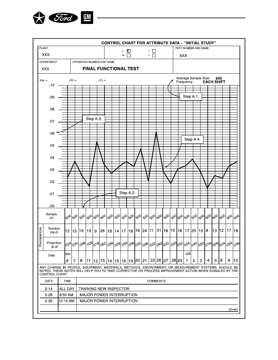
- 92 -

Figure 32. p Chart for Proportion Nonconforming - Gathering Data

III. CONTROL CHARTS FOR ATTRIBUTES

Section 1. p Charts (Cont.)

A. GATHER DATA

A.1.

Select the Size, Frequency and Number of Subgroups (See Figure 32.)

Subgroup Size - Charts for attributes generally require quite large subgroup sizes (e.g., 50 to
200 or more) to be able to detect moderate shifts in performance. For the chart to show
analyzable patterns, the subgroup size should be large enough to have several nonconform-
ing items per subgroup (e.g., np

– > 5) . Note, however, that large subgroup sizes can be a

disadvantage if each subgroup represents a long period of process operation. It is most con-
venient if subgroup sizes are constant or if they vary by no more than ± 25%, but this need
not be the case. It is also helpful that the subgroup size be large enough relative to p

– to

generate a lower control limit so that assignable causes due to improvement may also be
noticed.

Subgroup Frequency - The subgrouping frequency should make sense in terms of production
periods, to aid in analysis and correction of problems found. Short time intervals allow faster
feedback, but may conflict with requirements for large subgroup sizes.

Number of Subgroups - The data collection period should be long enough to capture all the
likely sources of variation affecting the process. Generally, it should also include 25 or more
subgroups to give a good test for stability and, if stable, a reliable estimate of process perfor-
mance.

A.2.

Calculate Each Subgroup’s Proportion Nonconforming (p) (See Figure 82.)

The following data should be recorded for each subgroup:

The number of items inspected - n
The number of nonconforming items found - np

From these, calculate the proportion nonconforming:

p =

These data should be recorded on a data form as the basis of initial analysis. When the most
recent historical data are available, they may be used to accelerate this phase of the study.

A.3.

Select Scales for the Control Chart (See Figure 32.)

The chart on which the data are plotted should be laid out with the proportion (or percent)
nonconforming as the vertical scale, and the subgroup identification (hour, day, etc.) as the hori-
zontal scale. The vertical scale should extend from zero to about 1-1/2 to 2 times the highest
proportion nonconforming noted in the initial data readings.

A.4.

Plot the Proportion Nonconforming on the Control Chart (See Figure 32.)

Plot the values of p for each subgroup. It is usually helpful to connect the points with lines to help
visualize patterns and trends.

As the points are plotted, briefly scan them to see if they are reasonable. If any points are sub-
stantially higher or lower than the others, co ,firm that the calculations are correct.

Record changes in the process, or unusual occurrences that may affect the process, as they are
observed, in the “comments” section of the chart.

- 93 -

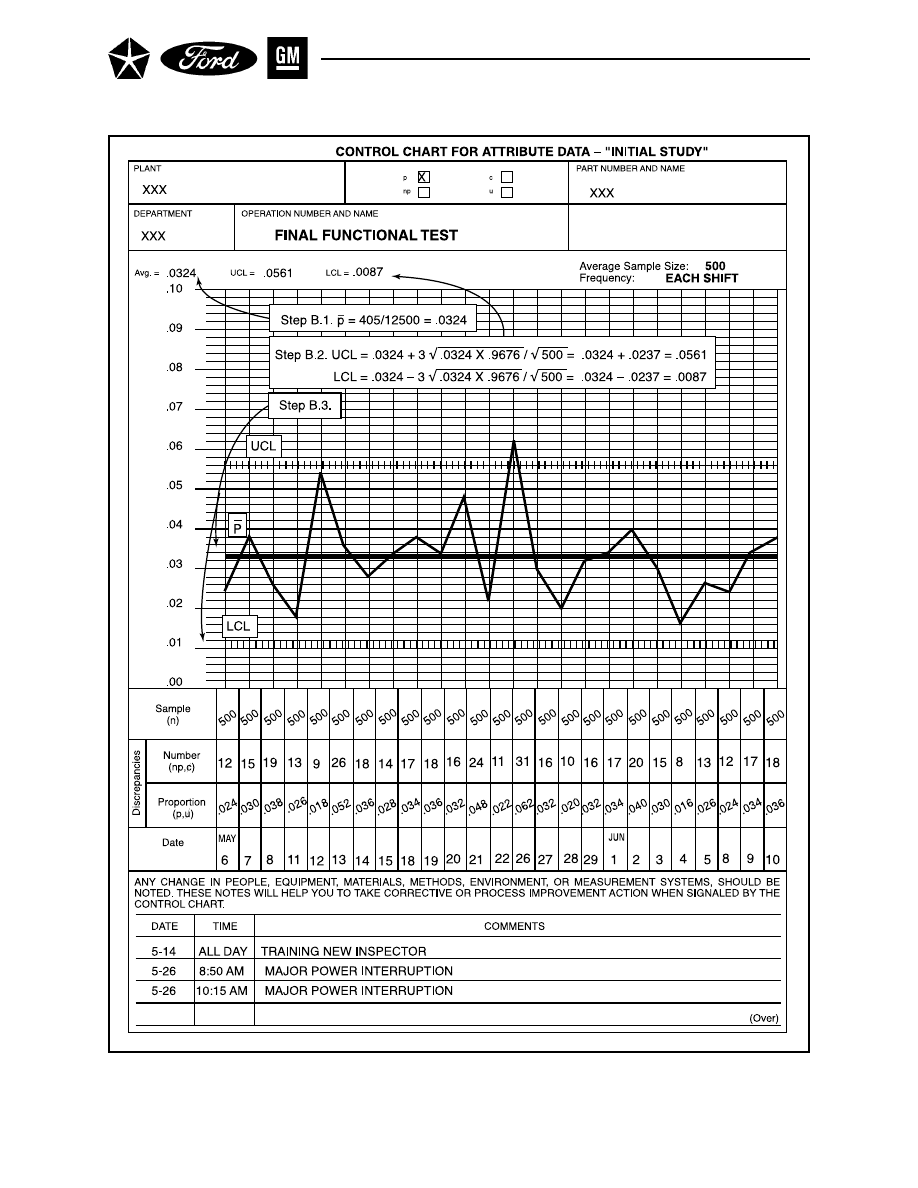
- 94 -

Figure 33. p Chart for Proportion Nonconforming - Calculating Control Limits, Sheet 1

III. CONTROL CHARTS FOR ATTRIBUTES

Section 1. p Charts (Cont.)

B. CALCULATE CONTROL LIMITS

B.1.

Calculate the Process Average Proportion Nonconforming ( p

–

) (See Figure 33,

Sheet 1.)

For the study period of k subgroups, calculate the average proportion nonconforming

–

+ n

= ... + n

+ n

+ ... + n

where n

, n

... and n

, n

... are the number of nonconforming items and number of items

inspected in each subgroup. Care should be taken not to confuse percentages (p x 100) with
proportion defective (p).

B.2.

Calculate the Upper and Lower Control Limits (UCL, LCL) (See Figure 33, Sheet 1.)

The control limits are the process average plus or minus an allowance for the variation that
could be expected if the process were in statistical control, given the subgroup sample size.
For the study period of k subgroups, calculate the upper and lower control limits:

UCL

= p

–

+ 3

√

p (1 - p

–

) /

√

LCL

= p

–

+ 3

√

p (1 - p

–

) /

√

where n is the constant sample size.

Note: When p

–

is low and/or n is small, the LCL can sometimes be calculated as a negative

number. In these cases there is no lower control limit, since even a value of p = 0 for a particu-
lar period is within the limits of random variation.

B.3.

Draw and Label Lines (See Figure 33, Sheet 1.)

•

Process Average (p

–

)-solid horizontal line

•

Control Limits (UCL, LCL)-dashed horizontal lines

During the initial study phase, these are considered trial control limits.

- 95 -

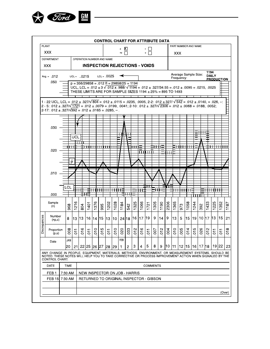
- 96 -

Figure 33. p Chart for Proportion Nonconforming - Calculating Control Limits, Sheet 2

III. CONTROL CHARTS FOR ATTRIBUTES

Section 1. p Charts (Cont.)

NOTE

The control limit calculations given above are appropriate when the subgroup sizes
are all equal (as they would be in a controlled sampling situation). Theoretically,
whenever the sample size changes (even for a single subgroup), the control limits
change, and unique limits would be calculated for each subgroup having a unique
sample size. However, for practical purposes, control limits calculated with an
average sample size (n

–

) are acceptable when the individual subgroup sizes vary

from the average by no more than plus or minus 25% (typical of actual production
volumes under relatively stable conditions). For these situations,

UCL

, LCL

= p

–

± 3

√

–

(1 - p

–

/ n

–

. When subgroup sizes vary by more than this

amount, separate control limits are required for the periods with particularly
small or large samples. A reasonable procedure (which should be documented in
the “comments” section of the form) is:

• Determine the range of sample sizes that would vary from the average by plus and minus

25%; identify all subgroups with sample sizes that lie outside this range.

• Recalculate the precise limits for those points as follows:

UCL

, LCL

= p

–

± 3

√

–

(1 - p

–

) /

√

n = p

–

± 3

√

–

(1 - p

–

) / n

where n is the sample size of the particular subgroup. Only the n term changes from point to
point.

• Plot the new upper and lower limits on the chart (see Figure 33, Sheet 2) for the affected

subgroups and use as the basis for identifying special causes.

Note that any procedure for handling variable control limits is going to be cumbersome and may
lead to potential confusion among people trying to interpret the charts. It is much better, wher-
ever possible, to structure the data collection plan so that constant sample sizes can be used.

- 97 -

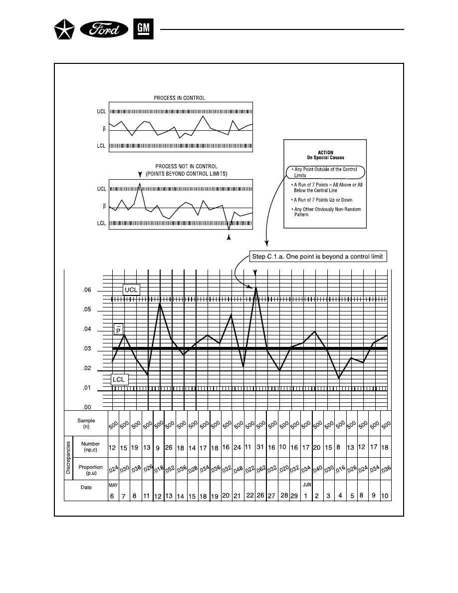
- 68 -

Figure 34. p Chart for Proportion Nonconforming - Points Beyond Control Limits

III. CONTROL CHARTS FOR ATTRIBUTES

Section 1. p Charts (Cont.)

C. INTERPRET THE CHART FOR PROCESS CONTROL

Objective: identify any evidence that the process is no longer operating at the same level-that it is out
of control-and to take appropriate action. Points beyond control limits, or obvious trends or patterns in
the data beyond what would likely occur due to chance, suggest the presence of special causes of varia-
tion.

C.1.

Analyze the Data Plots for Evidence of Instability

Points Beyond the Control Limits (See Figure 34.)-The presence of one or more points
beyond either control limit is evidence of instability at that point. Since points beyond
the control limits would be very rare if the process were stable and only common-cause
variation were present, we presume that a special cause has accounted for the extreme
value. The special cause may be either unfavorable or favorable; either situation bears
immediate investigation. This is the primary decision rule for action on any control chart.
Any point beyond the control limits should be marked.

A point above the upper control limit (higher proportion nonconforming) is generally a
sign of one or more of the following:

• The control limit or plot point are in error.
• The process performance has worsened, either at that point in time or as part of a trend,
• The evaluation system has changed (e.g., inspector, gage).

A point below the lower control limit (lower proportion nonconforming) is generally a
sign of one or more of the following:

• The control limit or plot point are in error.
• The process performance has improved (this should be studied for improvements that

might be incorporated on a permanent basis).

• The measurement system has changed.

Patterns or Trends Within the Control Limits- The presence of unusual patterns or trends,
even when all points are within the control limits, can be evidence of noncontrol or change
in level of performance during the period of the pattern or trend. This can give advance
warning of conditions which, if left uncorrected, could cause points beyond the control
limits.

NOTE:

When the average number of nonconforming items per subgroup (np

–

) is moderately

large (9 or more), the distribution of the subgroup p’s is nearly normal and trend
analysis similar to that used for X

–

charts can be used. When np

–

becomes small (5 or

fewer), the following rules are not directly applicable.

- 99 -

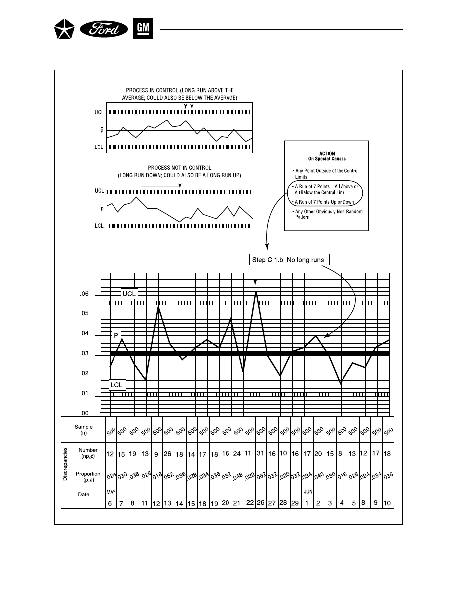
- 100 -

Figure 35. p Chart for Proportion Nonconforming - Runs

- 101 -

III. CONTROL CHARTS FOR ATTRIBUTES

Section 1. p Charts (Cont.) - Interpret for Control

Runs (See Figure 35.) — In a process under control, with np moderately large, approxi-
mately equal numbers of points should fall on either side of the average. Either of the
following could be a sign that a process shift or trend has begun:

• 7 points in a row on one side of the average.

• 7 points in a row that are consistently increasing (equal or greater than the preceding

points) or consistently decreasing.

In these cases, the point that prompts the decision should be marked (e.g., the seventh
point above the average); it may be helpful to extend a reference line back to the begin-
ning of the run. The analysis should consider the approximate time at which it appears
that the trend or shift first began.

Runs above the process average, or runs up, generally signify one or both of the following:

• The process performance has worsened-and may still be worsening.

• The evaluation system has changed.

Runs below the process average, or runs down, generally signify one or both of the fol-
lowing:

• The process performance has improved (the causes should be studied for permanent

incorporation).

• The evaluation system has changed.

NOTE:

When np

–

is small (below 5), the likelihood of runs below p

–

increases, so a run

length of 8 or more could be necessary to signal a decrease in the proportion
nonconforming.

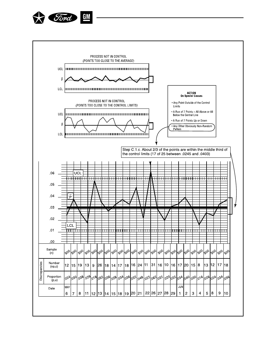
- 102 -

Figure 36. p Chart for Proportion Nonconforming - Nonrandom Patterns

III. CONTROL CHARTS FOR ATTRIBUTES

Section 1. p Charts (Cont.) - Interpret for Control

Obvious Nonrandom Patterns (See Figure 36.) — Other distinct patterns may indicate
the presence of special causes of variation, although care must be taken not to over-
interpret the data. Among these patterns are trends, cycles, unusual spread of points
within the control limits, and relationships among values within subgroups (e.g., if all
nonconforming items occur within the first few readings taken for the subgroup). One
test for unusual spread is given below:

Distance of points from the process average: Generally, in a process under statistical
control, with only common-cause variation present and np

–

moderately large, about 2/3

of the data points will be within the middle third of the region between the control limits;
about 1/3 of the points will be in the outer two-thirds of the region; about 1/20 will lie
relatively close to the control limits (in the outer third of the region).

If substantially more than 2/3 of the points lie close to the process average (for 25 sub-
groups if over 90% are within the middle third of the control limit region), this could
mean one or more of the following:

• The control limits or plot points have been miscalculated or misplotted.
• The process or the sampling method are stratified; each subgroup systematically con-

tains measurements from two or more process streams that have very different aver-
age performance (e.g., the mixed output of two parallel production lines).

• The data have been edited (values that would have deviated much from the average

have been altered or removed).

If substantially fewer than 2/3 of the points lie close to the process average (for 25 sub-
groups if 40% or fewer are in the middle third), this could mean one or both of the following:

• Calculation or plotting errors have been made.
• The process or the sampling method cause successive subgroups to contain measure-

ments from two or more process streams that have very different average perfor-
mance (e.g., performance differences between shifts).

If several process streams are present, they should be identified and tracked separately.

- 103 -

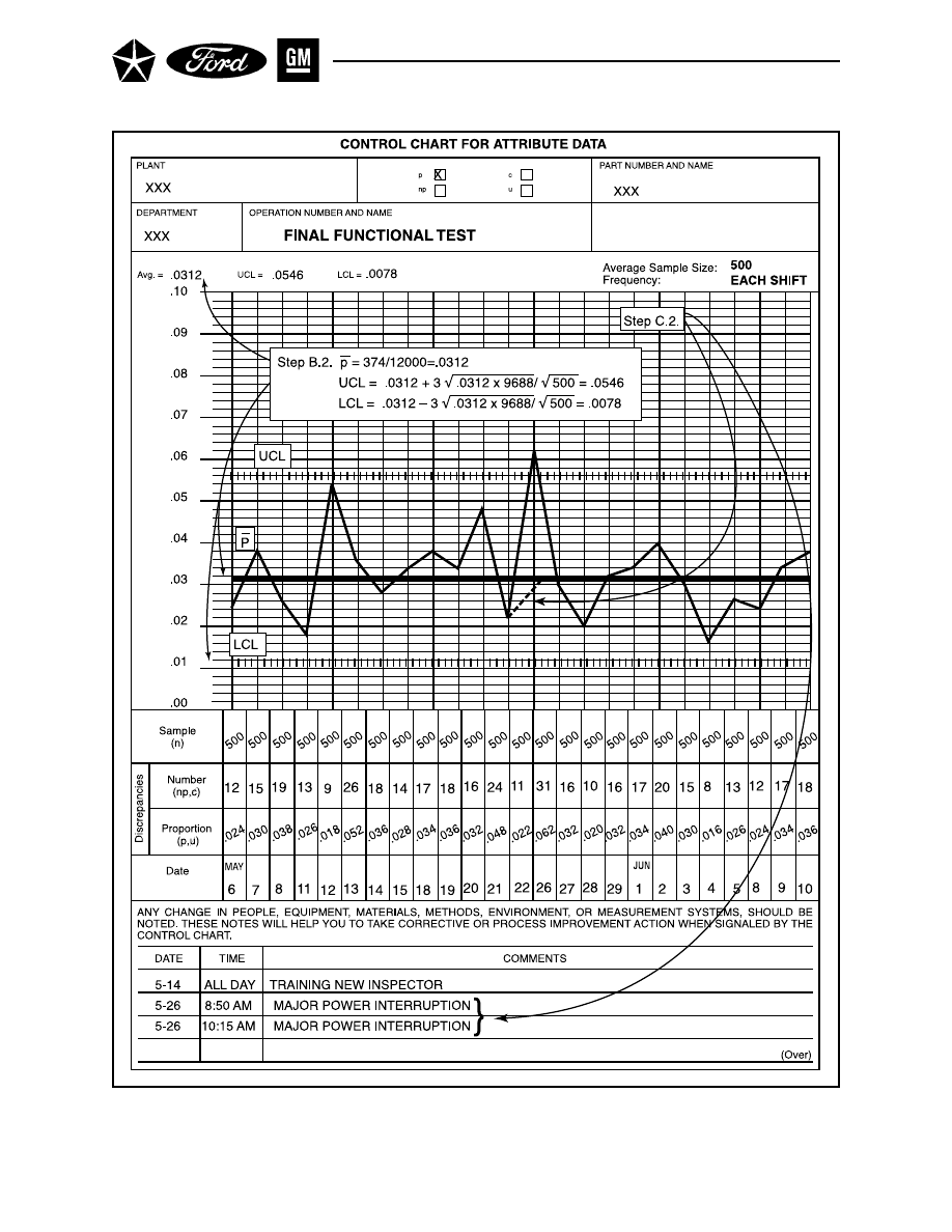
- 104 -

Figure 37. p Chart for Proportion Nonconforming - Control Limits Recalculation

III. CONTROL CHARTS FOR ATTRIBUTES

Section 1. p Charts (Cont.) - Interpret for Control

C.2.

Find and Correct Special Causes (See Figure 37.)

When an out-of-control condition has been identified in the data, the operation of the process
must be studied to determine the cause. This cause must then be corrected and, to the extent
possible, prevented from recurring. Since a special cause was indicated by the control chart,
analysis of the operations is called for, and one would often expect to find causes of variation
within the ability of the operator or local supervision to correct. Problem solving techniques
such as Pareto analysis and cause-and-effect analysis can be helpful (see Appendix H, Refer-
ence 11).

For ongoing studies being made with real-time data, analysis of out-of-control conditions in-
volves the timely investigation of the operation of the process, with emphasis on finding what,
if any, changes occurred that might explain the abnormal performance. When this analysis
has resulted in corrective action, the effectiveness of the action should become apparent in the
control chart.

For preliminary studies with historical data, the passage of time may make analysis of pro-
cess operating changes more difficult, especially for symptoms that come and go. The analysis
must be made as well as possible under the circumstances, to identify the condition and to
prevent its recurrence. A well documented “comments” section could be very helpful in this
regard.

C.3.

Recalculate Control Limits (See Figure 37.)

When conducting an initial process study or a reassessment of the process capability, the trial
control limits may need to be recalculated to exclude the effects of periods whose state of
control was affected by special causes which have been corrected. The control limits should be
recalculated excluding the points associated with the special causes and plotted on the chart
per paragraph B of this section. This step prevents abnormal production periods from being
included in the estimate of typical variability. The historical data should again be checked
against the revised limits to confirm that no further points suggest the presence of assignable
causes.

Once the historical data show consistent performance within the trial control limits, the lim-
its can be extended forward to cover future periods. They become the operating control limits
against which the future data will be evaluated as it is gathered and recorded.

The limits for ongoing control may be altered from those developed during the analysis period
by changing the sample size. In such a case, the basic formulas from paragraphs B.1. and B.2.
are used, but with the desired sample size n

new

, instead of n

–

Note:

For more extensive discussions of interpretation, tests for randomness in data, and prob-
lem solving, see Appendix H, References 6 through 12.

- 105 -

- 106 -

CALCULATE THE PROCESS CAPABILITY

From the example:

– = .0312

Process capability currently is 3.12% failures of the functional
check (96.88% OK).

EVALUATE THE PROCESS CAPABILITY

If the functional check is performed 100% and nonconforming
products are set aside, the customer is being protected from
receiving nonconforming product, but the 3% average failure
rate (requiring rework or scrap) is wasteful. Actions to improve
the chronic performance level should be developed.

III. CONTROL CHARTS FOR ATTRIBUTES

Section 1. p Charts (Cont.)

D. INTERPRET FOR PROCESS CAPABILITY

When control issues have been resolved, (special causes identified, analyzed and, where appropriate,
corrected/prevented from recurring) the control chart reflects the underlying process capability. For the
p chart (and all other attribute charts), process capability differs from that for variables data in the
sense that each point on an attribute chart directly indicates percent or rate of product nonconforming
(out-of-specifications) to customer requirements, whereas points on a variables chart indicate what the
process is yielding irrespective of engineering specifications. Therefore, for attribute charts, capability
is defined simply as the average proportion or rate of nonconforming product, whereas capability for
variables charts refers to the total (inherent) variation (6 σ

–

/d2

)yielded by the (stable) process, with

and/or without adjustments for process centering to specification targets.

D.1.

Calculate the Process Capability

• For a p chart, the process capability is reflected by the process average nonconforming, p

–

calculated when all points are in control. If desired, this can be expressed as the proportion
conforming to specification (1 - p

–

• For a preliminary estimate of process capability, use historical data, but exclude data

points associated with special causes.

• For a formal process capability study, new data should be run, preferably for 25 or more

periods, with the points all reflecting statistical control. The p

–

for these consecutive in-

control periods is a better estimate of the process’s current capability.

D.2.

Evaluate the Process Capability

• The process capability as just calculated reflects the ongoing level of performance that the

process is generating and can be expected to generate, as long as the process remains in
control and does not experience any basic change in performance. On a period-to-period
basis, the measured proportion nonconforming will vary between the control limits, but
barring any changes in the process, or periods allowed to go out of control, the average
proportion nonconforming will tend to be stable.

• This average capability, not the fluctuating individual values, must be evaluated against

management’s expectations for the particular characteristic. Then, if this average level is
unacceptable, further analysis and action must be directed toward the process itself (man-
agement responsibility).

- 107 -

- 108 -

IMPROVE THE PROCESS CAPABILITY

To improvehe chronic performance of the process, concentrate
on the common causes that affect all periods. These will usu-
ally require management action.

CHART AND ANALYZE THE REVISED PROCESS

Confirm the effectiveness of system changes by continude
monitoring of the control chart.

III. CONTROL CHARTS FOR ATTRIBUTES

Section 1. p Charts (Cont.) - Interpret for Process Capability

D.3.

Improve the Process Capability

• Once the process is demonstrating statistical control, the remaining average level of

nonconformities will reflect the systematic causes of variation in the underlying process-
the process capability. The types of analysis performed in diagnosing the special cause
(control) issues, which focused on operations, will no longer be appropriate in diagnosing
common causes affecting the system. Unless management action is directed toward the
system itself, no improvement in the process capability can be expected. Long-term solu-
tions are necessary to correct the sources of chronic nonconformities.

• Problem solving techniques such as Pareto analysis and cause-and-effect analysis can be

helpful (see Appendix H, Reference 11). However, understanding of the problems can be
difficult when only attributes data are used. In general, problem solving is aided by going
upstream in the process as far as possible toward the source of suspected causes of varia-
tion, and by using variables data for analysis (e.g., in X

–

and R charts).

D.4.

Chart and Analyze the Revised Process

• When systematic process actions have been taken, their effects should become apparent

in the control chart; the chart becomes a way of verifying the effectiveness of the action.

• As the process change is implemented, the control chart should be monitored carefully.

This change period can be disruptive to operations, potentially causing new control prob-
lems that could obscure the true effect of the system change.

• After any special causes of variation that appear during the change period have been

identified and corrected, the process will be in statistical control at a new process average.
This new average reflecting in-control performance can be used as the basis of ongoing
process control. However, investigation and improvement of the system should continue.

- 109 -

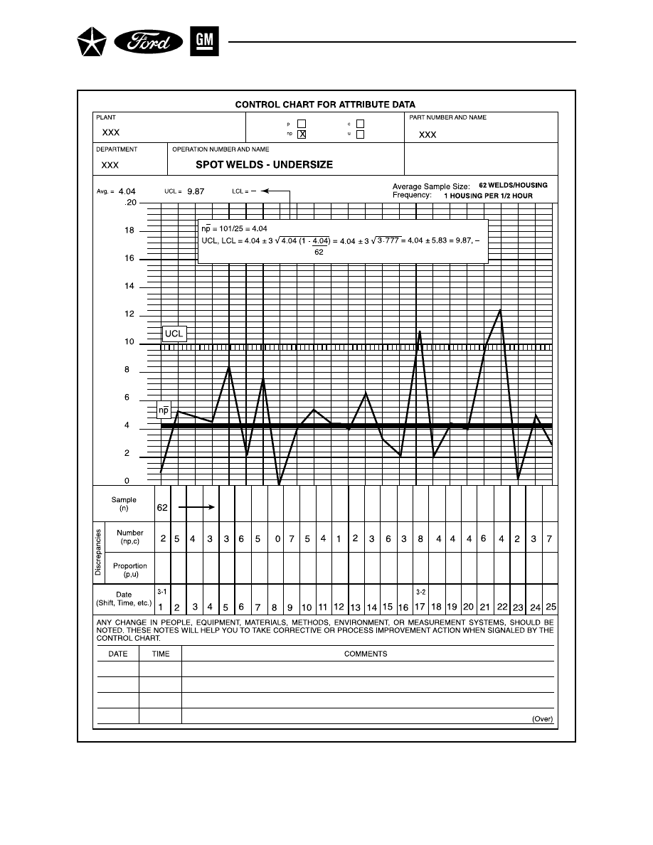
- 110 -

Figure 38. np Chart for Number Nonconforming

III. CONTROL CHARTS FOR ATTRIBUTES

Section 2

THE np CHART FOR NUMBER NONCONFORMING

The np chart (see Figure 38) measures the number of nonconforming (discrepant or so-called defective)
items in an inspection lot. It is identical to the p chart except that the actual number of nonconforming
items, rather than their proportion of the sample, is recorded. Both p and np charts are appropriate for
the same basic situations, with the choice going to the np chart if (a) the actual number of nonconformities
is more meaningful or simpler to report than the proportion, and (b) the sample size remains constant
from period to period. The details of instructions for the np chart are virtually identical to those for the
p chart; exceptions are noted below.

A. GATHER DATA

(See Section 1, Part A of this chapter; exceptions are noted below)

• The inspection sample sizes must be equal. The period of subgrouping should make sense in

terms of production intervals and feedback systems, and samples should be large enough to
allow several nonconforming items to appear in each subgroup. Record the sample size on the
form.

• Record and plot the number nonconforming in each subgroup (np).

B. CALCULATE CONTROL LIMITS

(See Section 1, Part B of this chapter; exceptions are noted below.)

• Calculate the Process Average Number Nonconforming ( np

–

n p

–

+ np

+ ... + np

where np

, np

... are the number nonconforming in each of the k subgroups.

• Calculate the Upper and Lower Control Limits (UCL, LCL).

UCL

= np

–

+ 3

√

–

(1 -

–

) = np

–

+ 3

√

–

(1 - p

–

)

LCL

= np

–

- 3

√

–

(1 -

–

) = np

–

- 3

√

–

(1 - p

–

)

where n = the subgroup sample size.

C. INTERPRET FOR PROCESS CONTROL

(See Section 1, Part C of this chapter.)

D. INTERPRET FOR PROCESS CAPABILITY

(See Section 1, Part D of this chapter). Note the process capability for an np chart is still p

–

, just as

it is for a p chart.

- 111 -

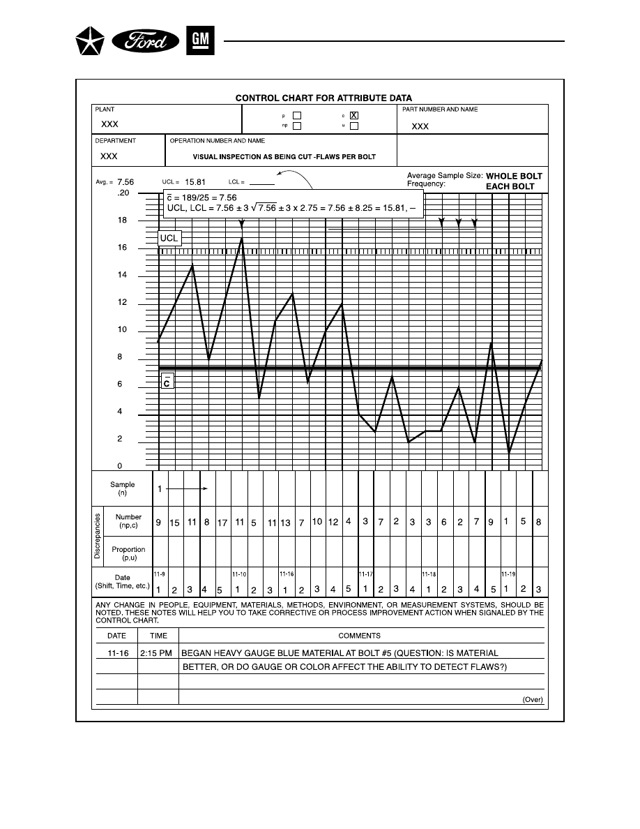
- 112 -

Figure 39. c Chart for Number Nonconformities

III. CONTROL CHARTS FOR ATTRIBUTES

Section 3

THE c CHART FOR NUMBER OF NONCONFORMITIES

The c chart (see Figure 39) measures the number of nonconformities (discrepancies or so-called defects)
in an inspection lot (as opposed to the number of units found nonconforming, as plotted on an np chart).
The c chart requires a constant sample size or amount of material inspected. It is applied in two major
types of inspection situations:

•

Where the nonconformities are scattered through a continuous flow of product (e.g., flaws in a bolt
of vinyl, bubbles in glass, or spots of thin insulation on wire), and where the average rate of
nonconformities can be expressed (e.g., flaws per 100 square meters of vinyl).

•

Where the nonconformities from many different potential sources may be found in a single inspec-
tion unit (e.g., the writeups at a departmental repair station, where each individual vehicle or
component could have one or more of a wide variety of potential nonconformities).

The following are the steps in construction and application of a c chart, which are similar to the basic
approach described previously for p charts; exceptions are noted below:

A. GATHER DATA

(See Section 1, Part A of this chapter; exceptions are noted below)

•

The inspection sample sizes (number of units, area of fabric, length of wire, etc.) need to be equal so
that the plotted values of c will reflect changes in quality performance (rate of occurrence of
nonconformities, c) rather than changes in exposure (the same size, n). Record the sample size on
the form.

•

Record and plot the number of nonconformities in each subgroup (c).

B. CALCULATE CONTROL LIMITS

(See Section 1, Part B of this chapter; exceptions are noted below)

•

Calculate the Process Average Number of Nonconformities (c

–

+ c

+ ... + c

where c

, c

... are the number of nonconformities in each of the k subgroups.

•

Calculate the Control Limits (UCL

and LCL UCL

)

UCLc = c

–

+ 3

√

–

LCLc = c

–

+ 3

√

–

C. INTERPRET FOR PROCESS CONTROL

(See Section 1, Part C of this chapter.)

D. INTERPRET FOR PROCESS CAPABILITY

(See Section 1, Part D of this chapter: exceptions are noted below)

The process capability is c

–

, the average number of nonconformities in a sample of fixed size n.

- 113 -

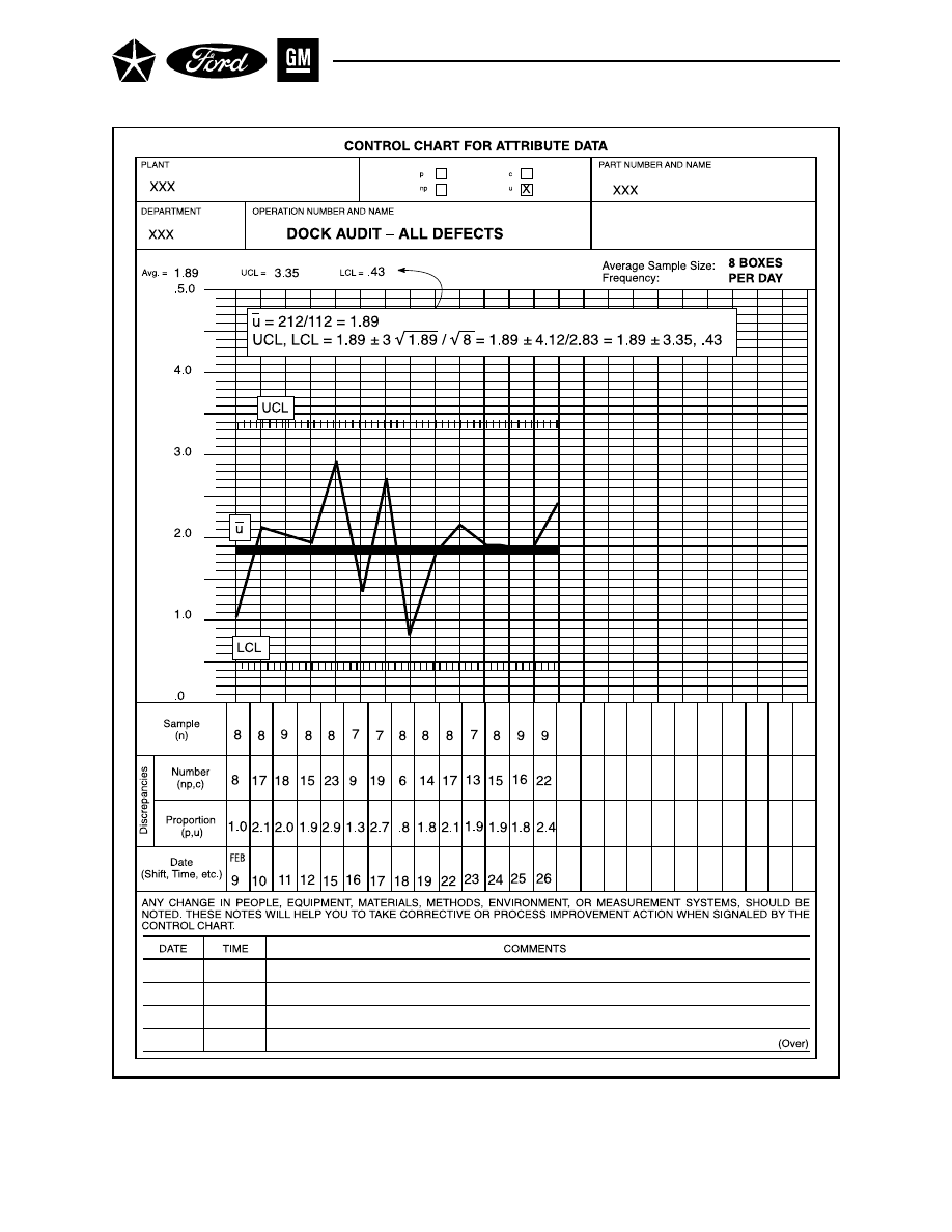
- 114 -

Figure 40. u Chart for Nonconformities Per Unit

III. CONTROL CHARTS FOR ATTRIBUTES

Section 4

THE u CHART FOR NONCONFORMITIES PER UNIT

The u chart (see Figure 40) measures the number of nonconformities (discrepancies or so-called de-
fects) per inspection reporting unit in subgroups which can have varying sample sizes (or amounts of
material inspected). It is similar to the c chart except that the number of nonconformities is expressed
on a per unit basis. Both u and c charts are appropriate for the same basic data situations; however, the
u chart may be used if the sample includes more than one “unit” (to make the reporting more meaning-
ful), and it must be used if the sample size can vary from period to period. The details of instructions for
the u chart are similar to those for the p chart; exceptions are noted below:

A. GATHER DATA

(See Section 1, Part A of this chapter; exceptions are noted below.)

• Sample sizes do not need to be constant from subgroup to subgroup, although maintaining them

within 25% above or below the average simplifies the calculation of control limits.

• Record and plot the nonconformities per unit in each subgroup (u):

u =

where c is the number of nonconformities found, and n is the sample size (number of inspection
reporting units) of the subgroup; c and n should also be recorded on the form.

NOTE:

The sample size for each subgroup, n, is expressed in terms of inspection reporting
units. Sometimes the reporting unit is a single production unit, e.g., an engine.
Often, however, the inspection reporting unit is other than one production unit. For
instance, in reports showing nonconformities per 100 units, the reporting unit is
100 production units, and n shows how many hundreds were inspected.

B. CALCULATE CONTROL LIMITS

(See Section 1, Part B of this chapter; exceptions are noted below.)

• Calculate the Process Average Nonconformities Per Unit (u

–

)

–

+ c

+ ... + c

+ n

+ ... + n

where c

, c

... and n

, n

... are the number of nonconformities and sample size of each of the k

subgroups.

Calculate the Control Limits (UCL and LCL)

UCL

= u

–

+ 3

√

–

√

–

= u

–

+ 3

√

–

LCL

= u

–

- 3

√

–

√

–

= u

–

- 3

√

–

where n

–

is the average sample size.

- 115 -

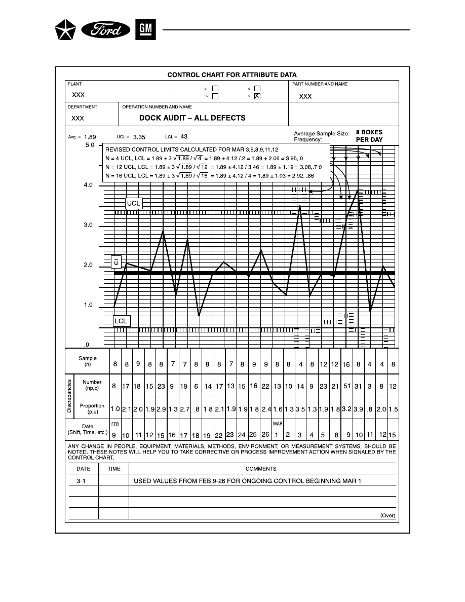
- 116 -

Figure 41. u Chart - Control Limits Recalculation

III. CONTROL CHARTS FOR ATTRIBUTES

Section 4. U Charts (Cont.) - Calculate Control Units

NOTE:

(See Figure 41.) If any individual subgroup sample size is more than 25% above
or below the average sample size, recalculate the precise control limit as follows:

UCL

, LCL

+ u

–

± 3

√

–

√

n = u

–

± 3

√

–

where u

–

is the process average and n is the sample size (number of inspection

reporting units) of the particular subgroup. Change the limits on the chart and
use as the basis for identifying special causes.

Note that any use of variable control limits is cumbersome and potentially con-
fusing. It is much better wherever possible to avoid this situation by using con-
stant subgroup sample sizes.

C. INTERPRET FOR PROCESS CONTROL

(See Section 1, Part C of this chapter.)

D. INTERPRET FOR PROCESS CAPABILITY

(See Section 1, Part D of this chapter.)

The process capability is u

–

, the average number of nonconformities per reporting unit.

- 117 -

- 118 -

Chapter IV

PROCESS MEASUREMENT SYSTEMS ANALYSIS

Section 1

INTRODUCTION

Once the characteristic(s) to be measured is determined for a given process, an evaluation of the mea-
surement system for that characteristic(s) should be undertaken to ensure effective analysis of any
subsequent SPC data generated for that characteristic(s). Recall the fundamental finding shared by
statisticians and quality professionals throughout the world that an observed value is composed of a
master value of the characteristic being measured plus measurement error, or

observed value = master value + measurement error

“Measurement error” is a statistical term meaning the net effect of all sources of measurement vari-
ability that cause an observed value to deviate from the master value. Unfortunately, this relationship
means we are faced with making decisions about product using information (i.e., numbers) that con-
tains additional variability. Carrying this one step further, the total variability in a set of data consist-
ing of at least two measurements per lot (or subgroup) and many lots (subgroups) over time, is corre-
spondingly composed of two component parts, i.e.,

total variability = product variability + measurement variability *

The importance of minimizing the effect of measurement variability on assessments of process vari-
ability cannot be overstated. For a more complete understanding of the various aspects of the subject of
measurement systems analysis, please refer to the automotive industry’s Measurement System Analy-
sis (MSA) manual (Appendix H, Reference 15) published in December, 1990, by the Automotive Indus-
try Action Group (AIAG). One of the more straightforward and also widely applied methods of mea-
surement systems analysis presented in the ASQC Automotive Division/AIAG MSA Manual is pre-
sented here in this section as a reasonably well accepted approach for assessing a measurement system
prior to engaging in statistical process control. In no way is it meant to suggest that this is the only
acceptable MSA technique. Additionally, the technique presented here assumes the other key attributes
of a measurement system, i.e., accuracy, linearity, and stability, as described in the MSA Manual, have
been evaluated and deemed acceptable.

* Please see Appendix H, Reference 18.

- 119 -

- 120 -

IV. MEASUREMENT SYSTEMS ANALYSIS

Section 2

AVERAGE AND RANGE METHOD

The Average and Range method ( X

–

and R, sometimes referred to as the “Long Method”) is a mathemati-

cal method which will determine both repeatability and reproducibility for a measurement system.
This method will allow the measurement system to be decomposed into two separate components,
repeatability and reproducibility.

If repeatability is large compared to reproducibility, the reasons may be:

• The gage instrument needs maintenance.

• The gage should be redesigned to be more rigid.

• The clamping or location for gaging needs to be improved.

• There is excessive within-part variation.

If reproducibility is large compared to repeatability, then possible causes could be:

• The operator needs to be better trained in how to use and read the gage instrument.

• Calibrations on the gage dial are not clear.

• A fixture of some sort may be needed to help operator use the gage more consistently.

A. CONDUCTING THE STUDY

Although the number of operators, trials and parts may be varied, the subsequent discussion repre-
sents the optimum conditions for conducting the study. Refer to the gage R & R data sheet in Figure 42
on page 124. The detailed procedure is as follows:

Refer to the operators as A, B, and C and number the parts 1 through 10 so that the numbers
are not visible to the operators.

NOTE:

The ten parts should be randomly selected across a full range of the process - it is
important that the parts, in as much as is possible, be representative of the total
process (variation).

Calibrate the gage.

Let operator A measure 10 parts in a random order and have another observer enter the
results in row 1. Let operators B and C measure the same 10 parts without seeing each other’s
readings, then enter the results in rows 6 and 11, respectively.

Repeat the cycle using a different random order of measurement. Enter data in rows 2, 7 and
12. Record the data in the appropriate column. For example if the first piece gaged is part 7
then record the result in the column labeled part 7. If three trials are needed, repeat the cycle
and enter data in rows 3, 8 and 13.

Steps 3 and 4 may be changed to the following when large part size or simultaneous unavail-
ability of parts make it necessary:

Let operator A measure the first part and record the reading in row 1. Let operator B
measure the first part and record the reading in row 6. Let operator C measure the first
part and record the reading in row 11.

- 121 -

IV. MEASUREMENT SYSTEMS ANALYSIS

Section 2. Average and Range Method (Cont.) - Conducting the Study

Let operator A repeat reading on the first part and record the reading in row 2, operator
B record the repeat reading in row 7, and operator C record the repeat reading in row 12.
Repeat this cycle and enter the result in rows 3, 8 and 13, if three trials are to be used.

An alternative method may be used if the operators are on different shifts. Let operator A
measure all 10 parts and enter the readings in row 1. Then have operator A repeat the reading
in a different order and enter the results in rows 2 and 3. Do the same with operators B and C
on the other shift.

B. CALCULATIONS

The Gage Repeatability and Reproducibility calculations are shown on Figure 42 and Figure 43. Figure
42 shows the data sheet on which all study results are recorded. Figure 43 displays a report sheet on
which all identifying information is to be recorded and all calculations made according to the pre-
scribed formula. The procedure for doing the calculations after data has been collected is as follows:

Subtract the smallest reading from the largest reading in rows 1,2 and 3; enter the result in
row 5. Do the same for rows 6,7 and 8; and 11,12 and 13 and enter results in rows 10 and 15,
respectively. (Figure 42)

Entries in rows 5, 10 and 15 are made as positive values. (Figure 42)

Total row 5 and divide the total by the number of parts sampled to obtain the average range
for the first operators trials R

. Do the same for rows 10 and 15 to obtain R

–

and R

–

. (Figure 42)

Transfer the average of rows 5,10 and 15 ( R

–

) to row 17. Add them together and divide

by the number of operators and enter results as R (overall average range). (Figure 42)

Enter R (average value) in rows 19 and 20 and multiply by D

and D

, respectively, to get the

lower and upper control limits. Note D

is zero and D

is 3.27 if two trials are used. The value

of the Upper Control Limit (UCL

) of the individual ranges is entered in row 19. The value of

Lower Control Limit (LCL

) for less than seven trials is equal to zero. (Figure 42)

Repeat any readings that produced a range greater than the calculated UCLR using the same
operator and part as originally used, or discard those values and re-average and recompute R
and the limiting value UCLR based upon the revised sample size. Correct the special cause
that produced the out of control condition.

Sum the rows (rows 1,2, 3, 6, 7, 8, 11, 12, and 13). Divide the sum in each row by the number
of parts sampled and enter these values in the right most column labeled “Average”. (Figure
42)

Add the averages in rows 1,2 and 3 and divide the total by the number of trials and enter the
value in row 4 in the X

–

block. Repeat this for rows 6,7 and 8; and 11,12 and 13, and enter the

results in the blocks for X

–

and X

–

in rows 9 and 14, respectively. (Figure 42)

Enter the maximum and minimum averages of rows 4,9 and 14 in the appropriate space in
row 18 and determine the differences. Enter this difference in the space labeled X

–

DIFF

in row

18. (Figure 42)

- 122 -

IV. MEASUREMENT SYSTEMS ANALYSIS

Section 2. Average and Range Method (Cont.) Calculations

10. Sum the measurements for each trial, for each part, and divide the total by the number of

measurements (number of trials times the number of operators). Enter the results in row 16
in the spaces provided for part average. (Figure 42)

11. Subtract the smallest part average from the largest part average and enter the result in the

space labeled R

in row 16. R

is the range of part averages. (Figure 42)

12. Transfer the calculated values of R, X

–

DIFF

and R

to the blanks provided on the report side of

the form (Figure 43).

13. Perform the calculations under the column entitled “Measurement Unit Analysis” on the left

side of the form. (Figure 43).

14. Perform the calculations under the column entitled “% Process Variation” on the right side of

the form (Figure 43).

15. Check the results to make sure no errors have been made.

C. ANALYSIS OF RESULTS

The Gage Repeatability and Reproducibility Data Sheet and Report Form, Figure 42 and Figure 43,
will provide the method for analysis of gage study data. The analysis will estimate the variation and
percent of process variation for the total measurement system and its component’s repeatability, repro-
ducibility, and part-to-part variation. On the left side of the form (Figure 43) under Measurement Unit
Analysis, the 5.15 standard deviation spread which consumes 99% of the area under the normal curve
is calculated for each component of variation.

The repeatability or equipment variation (EV or σ e) is determined by multiplying the overall average
range ( R ) by a constant (K

). K

depends upon the number of trials used in the gage study.

The reproducibility or appraiser variation (AV or σ o is determined by multiplying the maximum aver-
age operator difference (X

–

DIFF

) by a constant (K

). K

depends upon the number of operators used in the

gage study. Since the appraiser variation is contaminated by the equipment variation, it must be ad-
justed by subtracting a fraction of the equipment variation. Therefore, the appraiser variation (AV) is
calculated by

AV =

√

–

DIFF

x K

]

[

(EV)

]

(n r)

where n = number of parts and r = number of trials. If a negative value is calculated under the square
root sign, the appraiser variation (AV) defaults to zero (0).

- 123 -

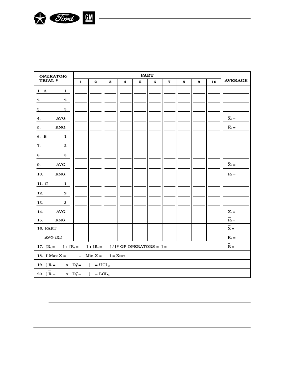
- 124 -

Figure 42. Gage Repeatability and Reproducibility Data Sheet

= 3.27 for 2 trials and 2.58 for 3 trials; D

= 0 for up to 7 tirals. UCL

represents the limit of individual R’s. Circle those that are

beyond this limit. Identify the cause and correct. Repeat these readings using the same appraiser and unit as originally used or
discard values and re-average and recompute R and the limiting value from the remaining observations.

Notes:

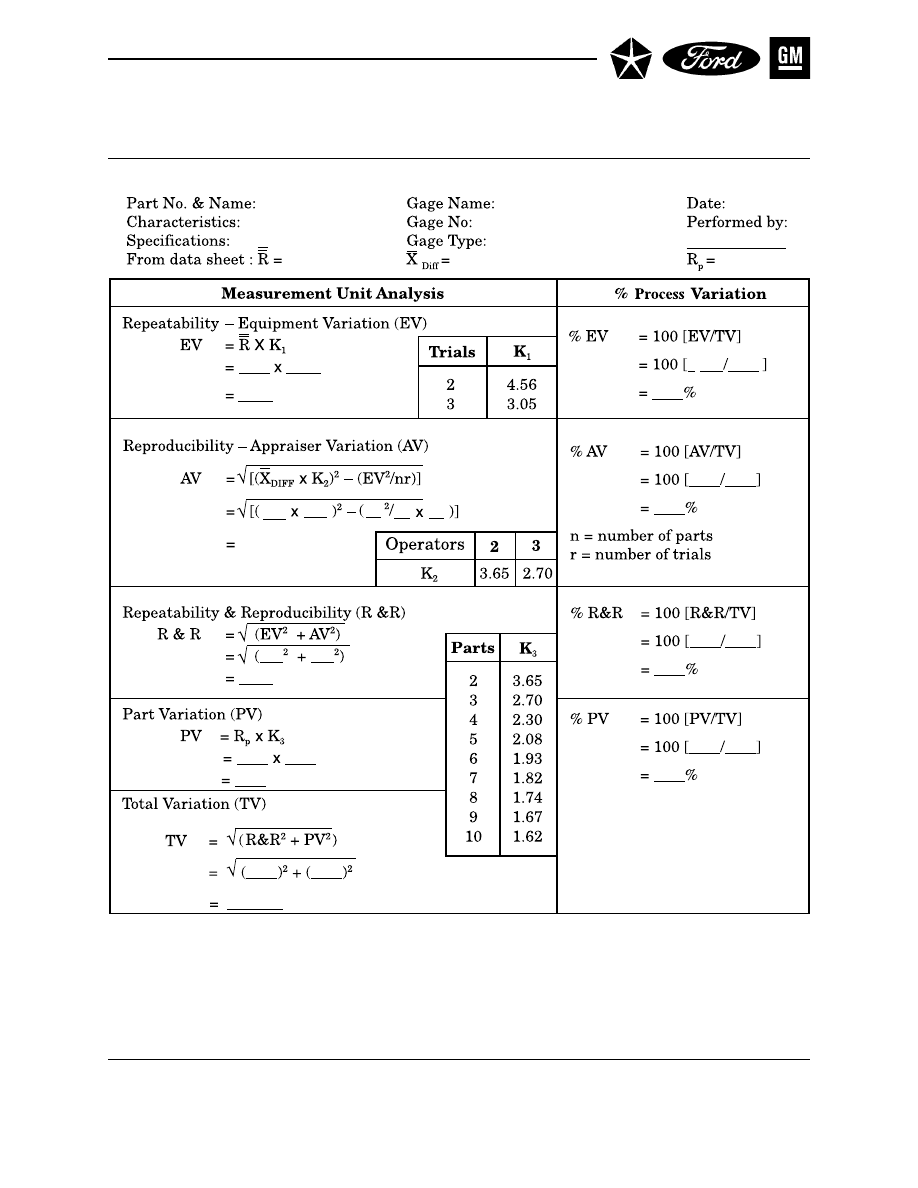
- 125 -

Figure 43. Gage Repeatability and Reproducibility Report

All calculations are based upon predicting 5.15 sigma (99.0% of the area under the normal distribution curve).
K

is 5.15/d

, where d

is dependent on the number of trials (m) and the number of parts times the numbe rof operators (g) which is

assumed to be greater than 15.d

values are from Appendix E.

AV - If a negative value is calculated under the square root sign, the appraiser variation (AV) defaults to zero (0).
K

is 5.15/d

*, where d

* is dependent on the number of operators (m) and (g) is 1, since there is only one range calculation.

is 5.15/d

*, where d

* is dependent on the number of parts (m) and (g) is 1, since there is only one range calculation./

* is obtained from Table D

, “Quality Control and Industrial Statistics,” A.J. Duncan. (See Appendix H, Reference 9).

IV. MEASUREMENT SYSTEMS ANALYSIS

Section 2. Average and Range Method (Cont.) - Analysis of Results

The measurement system variation for repeatability and reproducibility (R & R or σ

) is calculated by

adding the square of the equipment variation and the square of the appraiser variation, and taking the
square root as follows:

R & R =

√

[(EV)

+ (AV)

]

The part-to-part variation (PV or σ

) is determined by multiplying the range of part averages (R

) by a

constant (K

). K

depends upon the number of parts used in the gage study.

The total variation (TV or σ

) from the study is calculated by summing the square of both the repeat-

ability and reproducibility (R & R) variation and the part-to-part variation (PV) and taking the square
root as follows:

TV =

√

[(R & R)

+ (PV)

]

If the process variation is known and its value is based on 6σ , then it can be used in place of the total
study variation (TV) calculated from the gage study data. This is accomplished by performing the
following two calculations:

1. TV = 5.15

[

process variation

]

6.00

2. PV=

√

[(TV)

- (R & R)

]

Both of these values (TV and PV) would replace those previously calculated.

Once the variability for each factor in the gage study is determined, it can be compared to the total
variation (TV). This is accomplished by performing the calculations on the right side of the gage report
form (Figure 43) under “% Process Variation.”

The percent that the equipment variation (% EV) consumes of the total variation (TV) is calculated by

100

[

]

. The percent that the other factors consume of the total variation can be similarly calcu-

lated as follows:

% AV

= 100

[

]

%R&R

= 100

[

R & R

]

% PV

= 100

[

]

THE SUM OF THE PERCENT CONSUMED BY EACH FACTOR WILL NOT EQUAL 100%.

The results of this percent process variation should be evaluated to determine if the measurement
system is acceptable for its intended application.

- 126 -

IV. MEASUREMENT SYSTEMS ANALYSIS

Section 2. Average and Range Method (Cont.) Analysis of Results

If the analysis based on percent of tolerance is preferred instead of percent of process variation, then
the gage repeatability and reproducibility report form (Figure 43) can be modified so that the right
hand side of the form represents % of tolerance instead of % of process variation. In that case, % EV, %
AV, % R & R and % PV are calculated by substituting the value of tolerance in the denominator of the
calculations in place of the total variation (TV). Both approaches should be taken.

Guidelines for acceptance of gage repeatability and reproducibility (% R&R) using both approaches
described above are:

•

Under 10% error

Gage system O.K.

•

10% to 30% error

May be acceptable based upon importance of application, cost of gage,
cost of repairs, etc.

•

Over 30% error

Gage system needs improvement. Make every effort to identify the
problems and have them corrected.

D. EXAMPLE

The XYZ Corporation is starting an evaluation of measurement systems. The first measuring device to
be evaluated is a gasket thickness gage. The Quality Engineer decided to use ten parts to represent the
variability of the process, and three randomly selected operators from the inspector pool. Since time
was a constraint, only two trials would be performed. The method of data collection and analysis fol-
lows the procedures discussed earlier in this section with the results shown on Figure 44 and Figure 45.

The upper control limit (UCL

) and the lower control limit (LCL

) for the individual ranges are calcu-

lated as shown in Figure 44. The data could be plotted on a repeatability range control chart but
analysis of the range indicates that all ranges are in control (i.e., between the UCL

and LCL

). This

means all operators are consistent and are using the gage in the same way.

The measurement unit analysis and percent process variation for each component of variation must
then be calculated (see Figure 45). The results should be evaluated to determine if the measurement
system is acceptable for its intended application. In this example, the % R&R is 25.2% and therefore
the measurement system would be considered marginal for measuring the process variation.

- 127 -

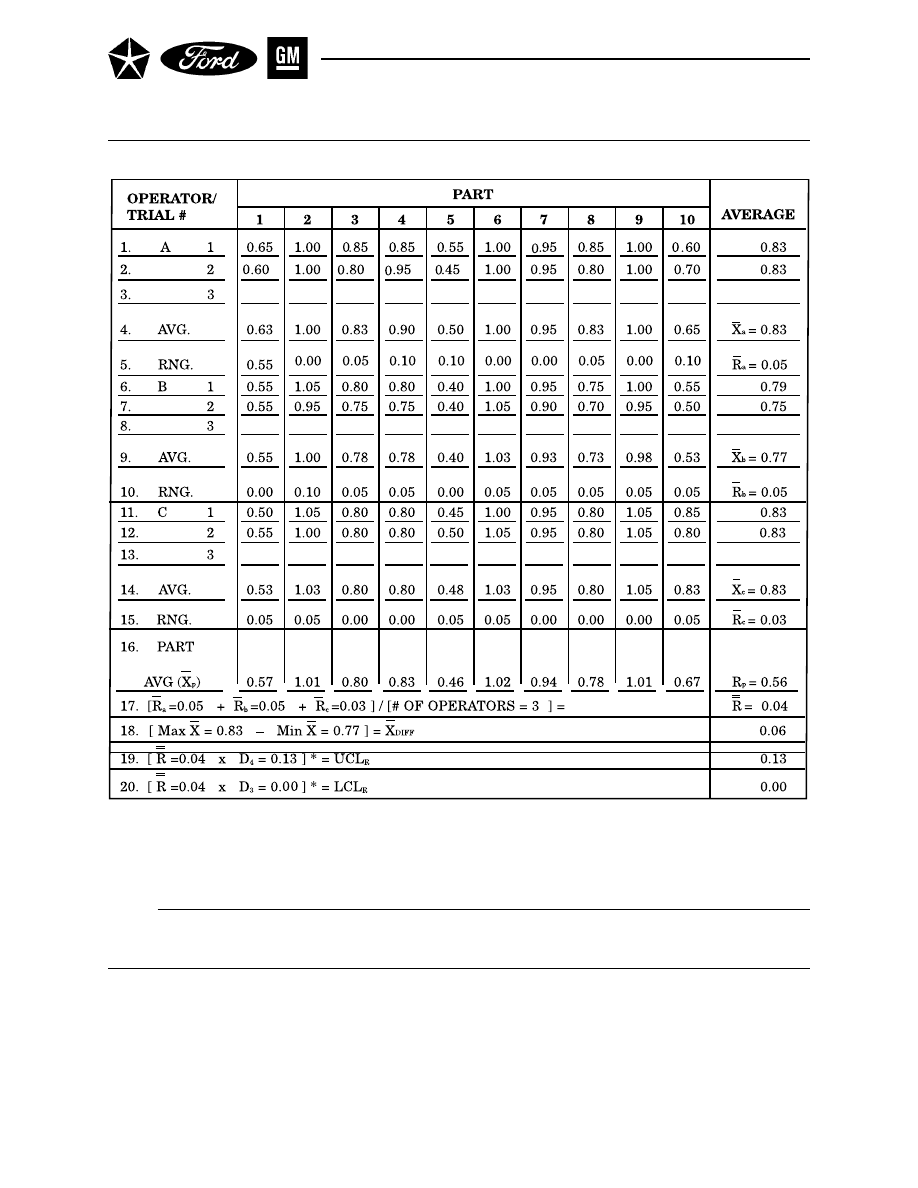
- 128 -

Figure 44. Gage Repeatability and Reproducibility Data Sheet - Example

= 3.27 for 2 trials and 2.58 for 3 trials; D

= 0 for up to 7 trials. UCL

represents the limit of individual

R’s. Circle those that are beyond this limit. Identify the cause and correct. Repeat these readings using
the same appraiser and unit as originally used or discard values and re-average and recompute R and the
limiting value from the remaining observations.

Notes:

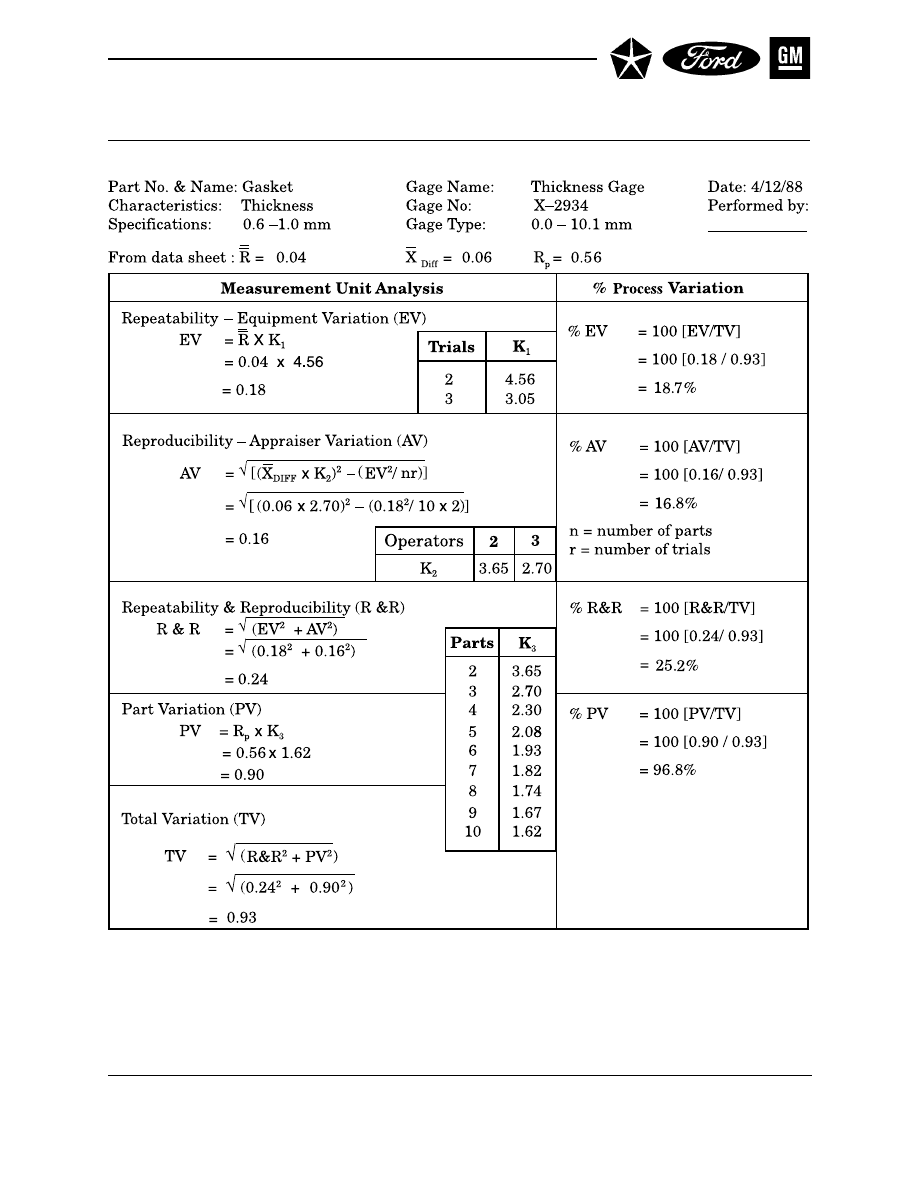
- 129 -

Figure 45. Gage Repeatability and Reproducibility Report - Example

All calculations are based upon predicting 5.15 sigma (99.0% of the area under the normal distribution curve).
K

is 5.15/d

, where d

is dependent on the number of trials (m) and the number of parts times the number of operators (g) which is

assumed to be greater than 15. d

values are from Appendix E.

AV - If a negative value is calculated under the square root sign, the appraiser variation (AV) defaults to zero (0).
K

is 5.15/d

*, where d

* is dependent on the number of operators (m) and (g) is 1, since there is only one range calculation.

is 5.15/d

*, where d

* is dependent on the number of parts (m) and (g) is 1, since there is only one range calculation.

* is obtained from table D

, “Quality Control and Industrial statistics,” A.J. Duncan. (See Appendix H, Reference 9).

- 130 -

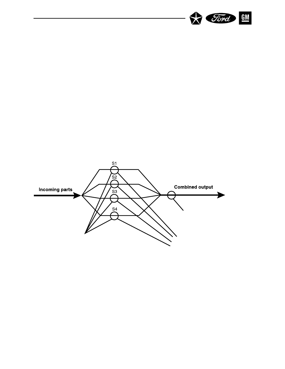
- 131 -

APPENDIX A

Some Comments on Subgrouping

Control charts are used to answer questions about a process. In order to have a control chart be useful it is
important that the charts answer the right questions. An X-bar chart asks the question, “Is the variation
present in subgroup averages more than is expected based on the variation within subgroups?”. Therefore,
understanding sources of variation within and between subgroups is of paramount importance in under-
standing the control chart and the process variation. Most variables control charts compare within sub-
group variation to between subgroup variation, so it is important in interpreting the control charts to form
subgroups with an understanding of the possible sources of variation affecting the process results. Con-
sider the following example: A production process consists of four parallel operations. It is suggested that
variation in process output should be studied with control charts, so a decision is to be made on how to
collect the data for the charts. There are a variety of possible sampling schemes that could be considered.
Parts could be taken from each stream to form a subgroup or parts from only one stream could be included
in the same subgroup or subgroups could be formed by taking parts from the combined stream of output
without regard to their source. The numerical example below provides an example of possible results
obtained using these three methods.

Methods to collect data from the output of a multiple stream (spindle) production process

Every hour a 16 part sample is collected by taking the parts from four consecutive cycles from each stream.
The following is an example of the data.

Cycle of the Machine
Sample #

Stream 1

Stream 2

Stream 3

Stream 4

There are three sources of variation captured in the data. Cycle to Cycle variation is captured by different
columns in the array, stream to stream variation is captured by the rows of the array, and hour-to-hour
variation is captured by different samples of 16 parts.

Method 1:

A subgroup consists

of one or more measurements
from each stream; this method of
subgrouping is stratified.

Method 2:

Collect data from each

stream separately. A subgroup
consists of measurements from only
one stream.

Method 3:

A subgroup

consists of measurements from
the combined output of all
streams.

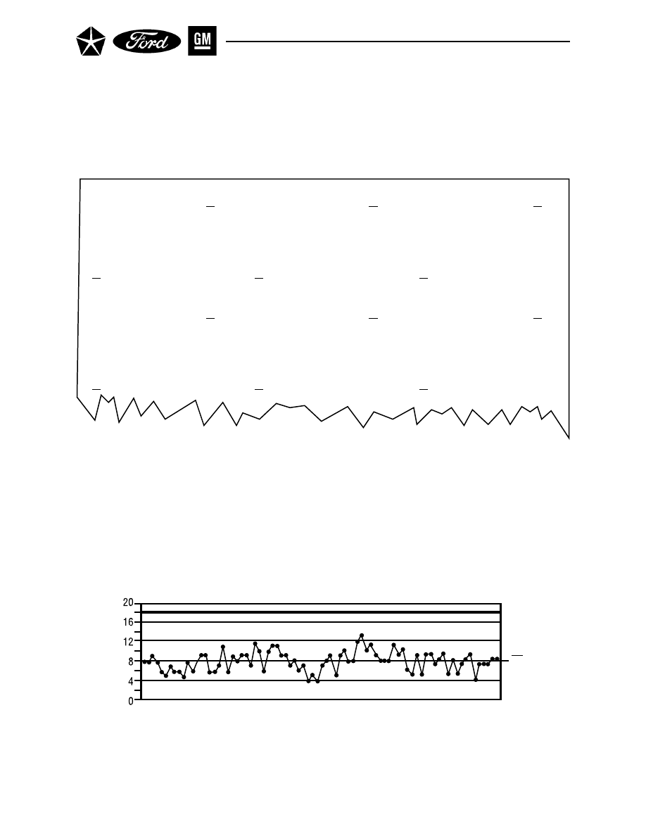
Appendix A Comments on Subgrouping (Cont.)

One subgrouping scheme would be to plot the average and range of each column of each array of data.
Using this subgrouping scheme, stream to stream variation would be contained within each subgroup.
Hour to hour variation and cycle to cycle variation would contribute to differences between subgroups.
Another possible subgrouping scheme would be to plot the average and range of each row of each array of
data. With this subgrouping scheme, cycle to cycle variation would be contained within each subgroup and
hour to hour and stream to stream variation would contribute to differences between subgroups.

- 132 -

Data from 20 consecutive hours are used to construct control charts with each subgrouping method.

Method 1: Subgrouping by column (Cycle)

This subgrouping scheme yields 80 subgroups of size n = 4. The average range is 7.85, and the upper
control limit for the range chart is 17.91 units. Within subgroup variation appears to be stable using this
method.

Range Chart for Data Subgrouped by Column (Cycle)

UCLR

10.0

S2 12

12.3

S3 17

18.3

S4 10

11.3

10.8

11.5

17.0

11.0

11.3

S3 15

16.5

S4 12

12.5

Subgrouping by column

X 12.0 13.5 12.8 14
R

6.8

8.3

S3 14

14.3

6.5

7.8

9.8

14.8

6.0

10.0

S2 13

14.0

S3 17

17.5

11.8

8.8

9.0

8.8 9.3

X 13.0 14.0 13.3 13.0
R

9.5 10.5 8.8 9.0

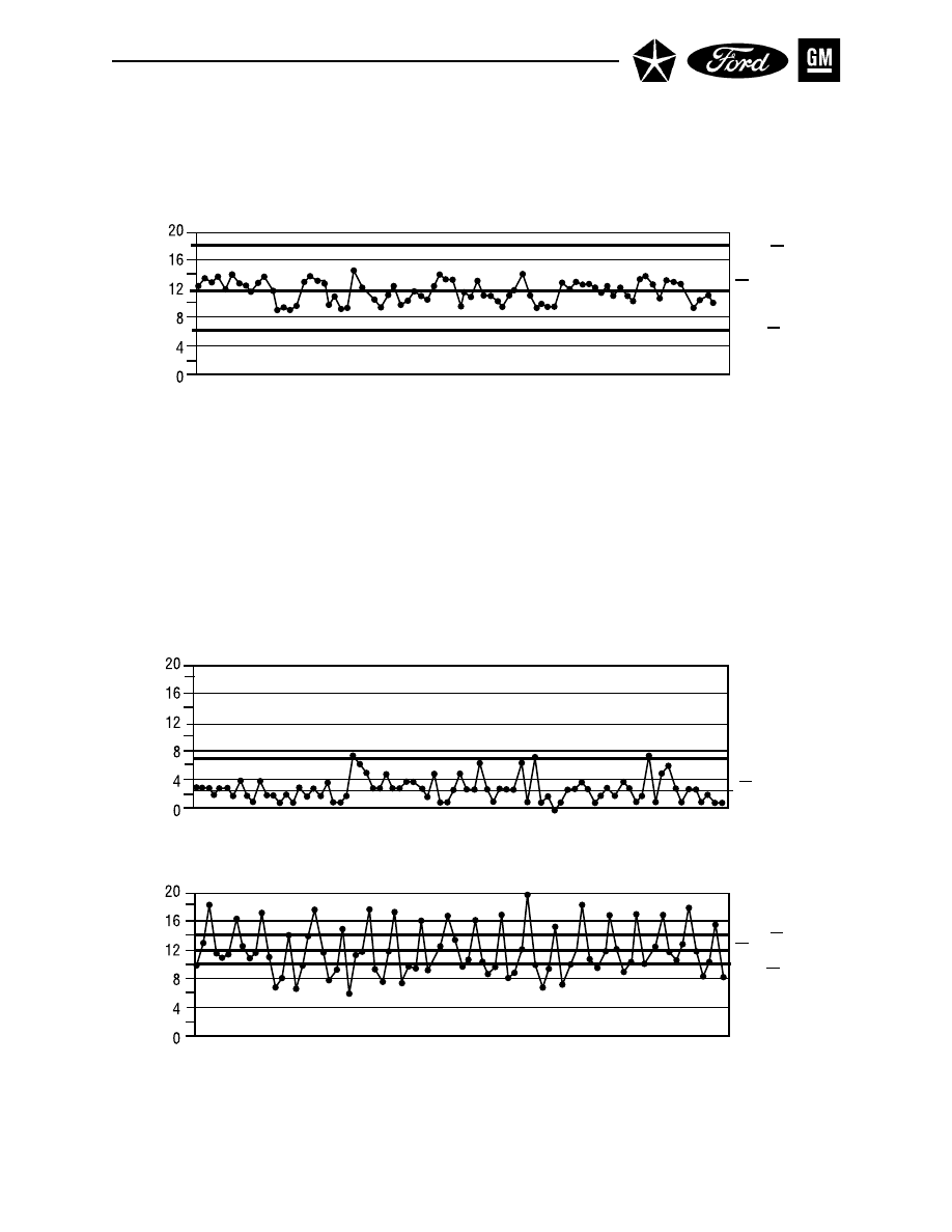
Appendix A Comments on Subgrouping (Cont.)

- 133 -

Method 2: Subgrouping by Row

The second subgrouping scheme yields 80 subgroups of size n = 4. The grand average is 11.76 units and the
average range is 2.84 units. The control limits for the X bar chart are 13.83 and 9.70 units, and the upper
control limit for the range chart is 6.46 units. The control charts for this subgrouping scheme are shown
below.

The control charts for the different subgrouping schemes are very different even though they are derived
from the same data. The X-bar chart for data subgrouped by row shows a pattern: All of the points corre-
sponding to spindle 3 are noticeably higher than those from the other streams. The first X-bar chart does
not reveal the stream differences because readings from each stream are averaged to obtain each X-bar
value. By grouping the date differently, the charts address different questions. For the first set of charts,

X-Bar Chart for Data Subgrouped by Column (Cycle)

UCL

LCL

Range Chart for Data Subgrouped by Row (Spindle)

X-Bar Chart for Data Subgrouped by Row (Spindle)

UCL

LCL

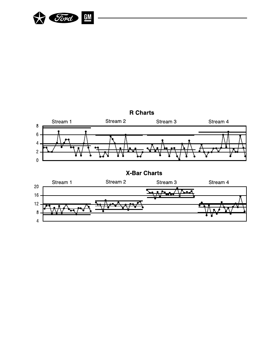
Appendix A Comments on Subgrouping (Cont.)

stream to stream variation is used as a basis of comparison. The R chart checks to see if stream to stream
variation is stable over time and the X-bar chart compares cycle to cycle and hour to hour with stream to
stream variation. The second set of charts use, cycle to cycle variation as a basis for comparison. The R
chart checks to see that the cycle to cycle variation is stable over time and the X-bar chart compares stream
to stream variation and hour to hour variation with the base level of variation established by the ranges—
i.e., cycle to cycle variation. Since the stream to stream differences are so large, the control limits in the
first set of charts are much wider than the second set.

With the second subgrouping method the data could be used to create four separate sets of control charts
from the data, one for each stream.

- 134 -

This comparison of the charts shows that the average of the third stream is higher than the others and the
individual processes are out of control. The base level of variation used for study of the results from each
stream is cycle to cycle variation as reflected in the range. For each stream the effects of hour to hour
variation are shown on the X-bar charts. By plotting the charts using the same scale, the level and varia-
tion for each stream can be compared.

Method 3: The third method of sampling would be to sample the parts from the combined output from all
four streams. This method gives some insight into the variation that is sent to the next process but, we can
no longer differentiate which stream produced the part. Provided the parts in the combined stream are
mixed, the ranges reflect a mixture of stream to stream and cycle to cycle variation. The X-bar values
contain, in addition, hour to hour variation. If the hour to hour contribution to variation is large enough,
that contribution will be seen as out of control points on the X-bar chart.

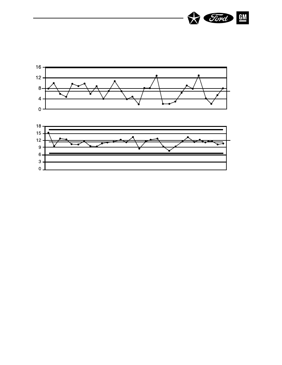
Appendix A Comments on Subgrouping (Cont.)

- 135 -

The R chart checks to see if stream to stream and cycle to cycle variation is consistent over time. The X-bar
chart answers the question, “Is the variation in X-bar values what would be expected if cycle to cycle and
stream to stream variation were the only kinds of variation present in the process, or, is there additional
change hour to hour?”

As a general rule, the variation that is represented within subgroups should be the kind of variation that
is believed to be the least significant or least interesting as a subject for current study. In all cases, a
method of subgrouping should be used that will allow questions about the effects of potential sources of
variation to be answered.

Combined Output R Chart

Combined Output X-Bar Chart

UCLR

–

UCLR

–

LCLX

–

- 136 -

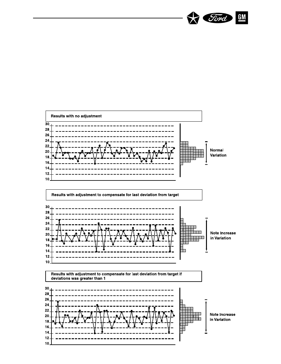
APPENDIX B

Overadjustment

Overadjustment is the practice of treating each deviation from the target as if it were the result of the
action of a special cause of variation in the process. If a stable process is adjusted on the basis of each
measurement made, then the adjustment becomes an additional source of variation. The following ex-
amples demonstrate this concept. The first graph shows the variation in results with no adjustment. The
second graph shows the variation in results when an adjustment is made to the process to compensate for
each deviation from the target. The third graph shows variation in results when adjustments are made to
compensate only when the last result was more than one unit from the target. This third case is an ex-
ample of compensation to stay within a set of specifications. Each method of adjustment increases the
variation in the output, since the variation without adjustment is stable (see Appendix H, Reference 4,
Chapter 11).

- 137 -

- 138 -

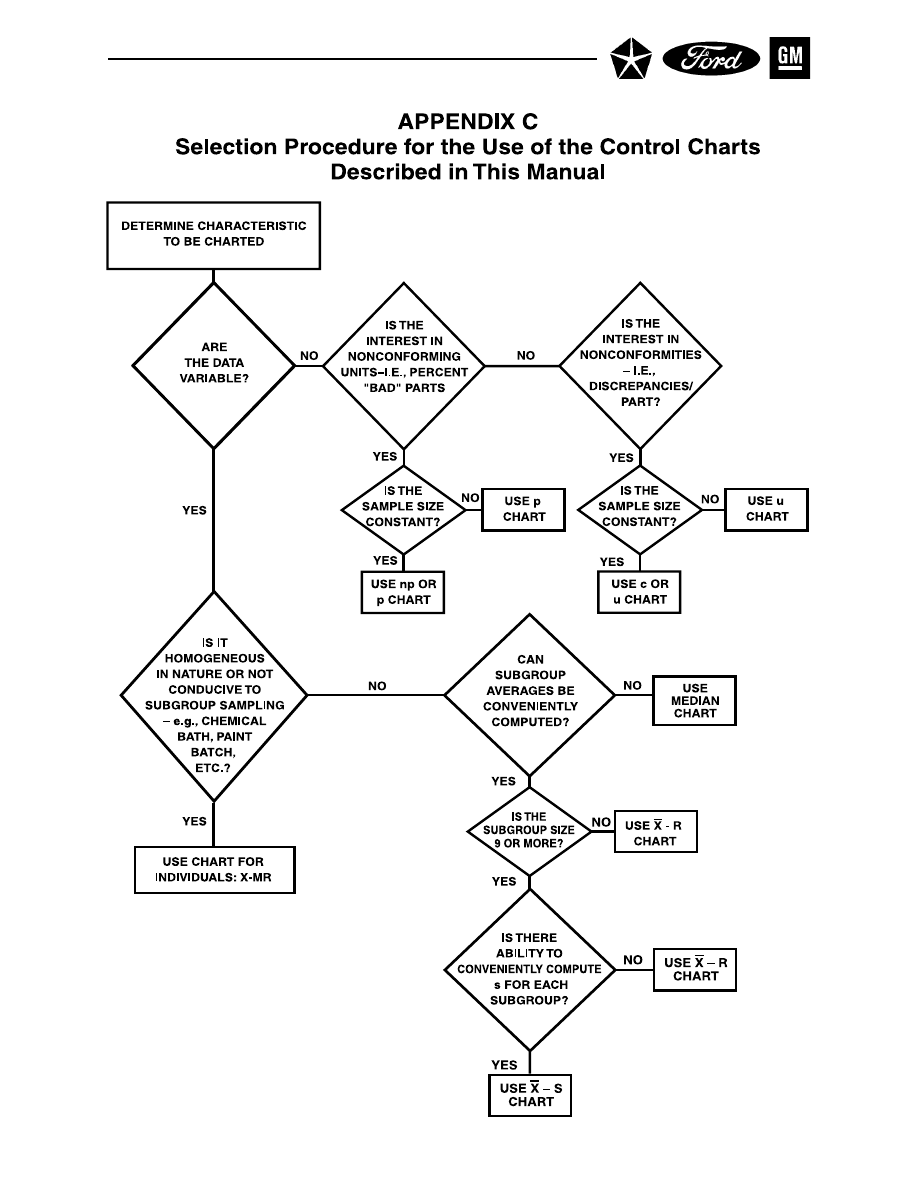
- 139 -

NOTE: This chart assumes the mea-
surement system has been assessed
and is appropriate

- 140 -

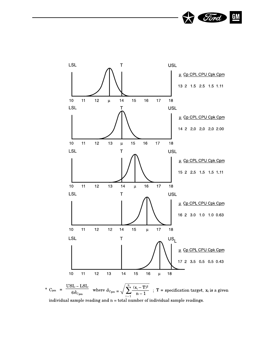
- 141 -

APPENDIX D

Relationship Between Cpm* and Other Indices With

(USL - T) = (T - LSL)**

** L.J. Chan, S.W. Cheng, and F.A. Spring, “A New Measure of Process Capability: C

,” Journal of

Quality Technology, Vol. 20, No. 3, July, 1989, p. 16. Reprinted from the Journal fo Quality Tech-
nology, A Publication of the American Society for Quality Control.

- 142 -

APPENDIX E

Table Of Constants and Formulas for Control Charts

–

and R Charts *

–

and s Charts *

Chart for

Averages

Charts for

–

)

Chart for Ranges (R)

–

)

Standard Deviations (s)

Divisors for

Factors for

Estimate of

Factors for

Estimate of

Factors for

Subgroup

Control

Standard

Control

Standard

Control

Size

Limits

Deviation

Limits

Deviation

Limits

1.880

1.128

–

3.267

2.659

0.7979

–

3.267

1.023

1.693

–

2.574

1.954

0.8862

–

2.568

0.729

2.059

–

2.282

1.628

0.9213

–

2.266

0.577

2.326

–

2.114

1.427

0.9400

–

2.089

0.483

2.534

–

2.004

1.287

0.9515

0.030

1.970

0.419

2.704

0.076

1.924

1.182

0.9594

0.118

1.882

0.373

2.847

0.136

1.864

1.099

0.9650

0.185

1.815

0.337

2.970

0.184

1.816

1.032

0.9693

0.239

1.761

0.308

3.078

0.223

1.777

0.975

0.9727

0.284

1.716

0.285

3.173

0.256

1.744

0.927

0.9754

0.321

1.679

0.266

3.258

0.283

1.717

0.886

0.9776

0.354

1.646

0.249

3.336

0.307

1.693

0.850

0.9794

0.382

1.618

0.235

3.407

0.328

1.672

0.817

0.9810

0.406

1.594

0.223

3.472

0.347

1.653

0.789

0.9823

0.428

1.572

0.212

3.532

0.363

1.637

0.763

0.9835

0.448

1.552

0.203

3.588

0.378

1.622

0.739

0.9845

0.466

1.534

0.194

3.640

0.391

1.608

0.718

0.9854

0.482

1.518

0.187

3.689

0.403

1.597

0.698

0.9862

0.497

1.503

0.180

3.735

0.415

1.585

0.680

0.9869

0.510

1.490

0.173

3.778

0.425

1.575

0.663

0.9876

0.523

1.477

0.167

3.819

0.434

1.566

0.647

0.9882

0.534

1.466

0.162

3.858

0.443

1.557

0.633

0.9887

0.545

1.455

0.157

3.895

0.451

1.548

0.619

0.9892

0.555

1.445

0.153

3.931

0.459

1.541

0.606

0.9896

0.565

1.435

UCL

–

, LCL

–

= X ± A

–

UCL

–

, LCL

–

= X ± A

s–

UCL

= D

–

UCL

= B

s–

LCL

= D

–

LCL

= B

s–

= R

–

= s–/c

From ASTM publication STP-15D, Manual on the Presentation of Data and Control Chart Analysis,
1976; pp 134-136. Copyright ASTM, 1916 Race Street, Philadelphia, Pennsylvania 19103. Reprinted,
with permission.

- 143 -

APPENDIX E - Table of Constants and Formulas for Control Charts (Cont.)

Median Cahrts, **

Charts for Individuals*

Chart for

Medians

Individuals

(X)

Chart for Ranges (R)

)

Chart for Ranges (R)

Divisors for

Factors for

Estimate of

Factors for

Estimate of

Factors for

Subgroup

Control

Standard

Control

Standard

Control

Size

Limits

Deviation

Limits

Deviation

Limits

1.880

1.128

3.267

2.660

1.128

3.267

1.187

1.693

2.574

1.772

1.693

2.574

0.796

2.059

2.282

1.457

2.059

2.282

0.691

2.326

2.114

1.290

2.326

2.114

0.548

2.534

2.004

1.184

2.534

2.004

0.508

2.704

0.076

1.924

1.109

2.704

0.076

1.924

0.433

2.847

0.136

1.864

1.054

2.847

0.136

1.864

0.412

2.970

0.184

1.816

1.010

2.970

0.184

1.816

0.362

3.078

0.223

1.777

0.975

3.078

0.223

1.777

UCL

, LCL

= X ± A

–

UCL

, LCL

= X ± E

–

UCL

= D

–

UCL

= D

–

LCL

= D

–

LCL

= D

–

= R

–

= R

–

* * A

Factors Derived from ASTM-STP-15D Data and Efficiency Tables Contained in W. J. Dixon and

F.J. Massey, Jr., Introduction to Statistical Analysis, Third Edition, 1969; Page 488; McGraw-Hill
Book Company, New York.

– ~

–

– ~

- 144 -

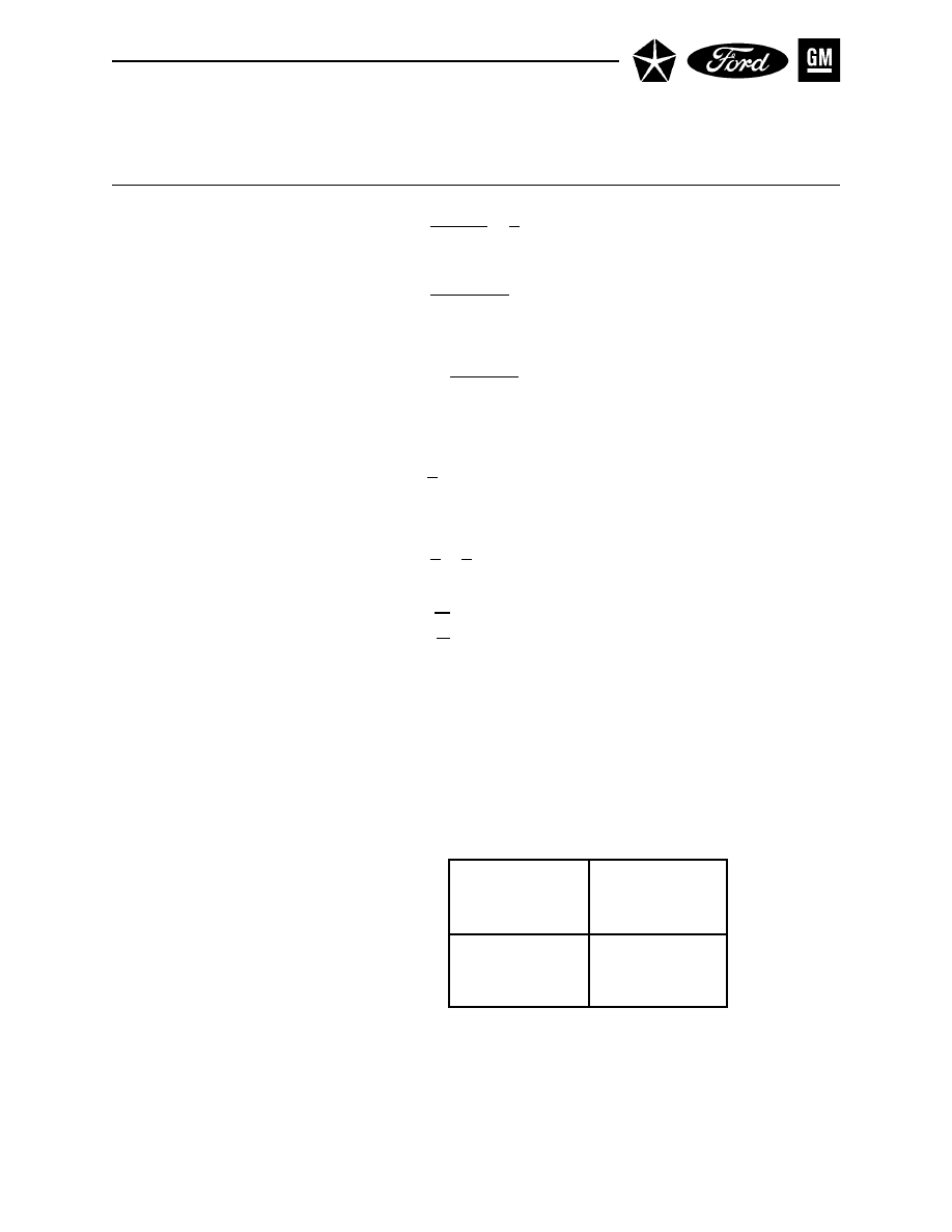
APPENDIX E - Table of Constants and Formulas for Control Charts (Cont.)

Attribute Charts

p chart for proportion of units nonconforming, from samples not necessarily of constant size:

UCL

, LCL

= p

– ± 3

√

– (1 - p–) /

√

= p

– ± 3

√

– (1 - p–) / n

np chart for number of units nonconforming, from samples of constant size:

UCL

, LCL

= np

– ± 3

√

– (1 - p–)

c chart for number of nonconformities, from samples of constant size:

UCL

, LCL

= c– ± 3

√

c–

u chart for number of nonconformities per unit, from samples not necessarily of constant size:

UCL

, LCL

= u

– ± 3

√

– /

√

= u

– ± 3

√

–

Memo: Guide for selection of charts for attributes:

NUMBER
(Simple, but needs
constant sample size)

PROPORTION
(More complex, but
adjusts to understandable
proportion, and can cope
with varying sample sizes)

- 145 -

Nonconforming

Units

Nonconformities

- 146 -

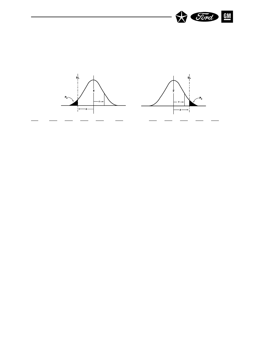
APPENDIX F

Standard Normal Distribution

= the proportion of process output beyond a particular value of interest (such as a specification limit)

that is z standard deviation units away from the process average (for a process that is in statistical control
and is normally distributed). For example, if z = 2.17, P

= .0150 or 1.5%. In any actual situation, this

proportion is only approximate.

|z|

x.x0

x.x1

x.x2

x.x3

x.x4

x.x5

x.x6

x.x7

x.x8

x.x9

4.0

.00003

3.9

.00005 .00005 .00004 .00004

.00004

.00004 .00004 .00004 .00003 .00003

3.8

.00007 .00007 .00007 .00006

.00006

.00006 .00006 .00005 .00005 .00005

3.7

.00011 .00010 .00010 .00010

.00009

.00009 .00008 .00008 .00008 .00008

3.6

.00016 .00015 .00015 .00014

.00014

.00013 .00013 .00012 .00012 .00011

3.5

.00023 .00022 .00022 .00021

.00020

.00019 .00019 .00018 .00017 .00017

3.4

.00034 .00032 .00031 .00030

.00029

.00028 .00027 .00026 .00025 .00024

3.3

.00048 .00047 .00045 .00043

.00042

.00040 .00039 .00038 .00036 .00035

3.2

.00069 .00066 .00064 .00062

.00060

.00058 .00056 .00054 .00052 .00050

3.1

.00097 .00094 .00090 .00087

.00084

.00082 .00079 .00076 .00074 .00071

3.0

.00135 .00131 .00126 .00122

.00118

.00114 .00111 .00107 .00104 .00100

2.9

.0019

.0018

.0017

.0016

.0015

.0014

2.8

.0026

.0025

.0024

.0023

.0022

.0021

.0020

.0019

2.7

.0035

.0034

.0033

.0032

.0031

.0030

.0029

.0028

.0027

.0026

2.6

.0047

.0045

.0044

.0043

.0041

.0040

.0039

.0038

.0037

.0036

2.5

.0062

.0060

.0059

.0057

.0055

.0054

.0052

.0051

.0049

.0048

2.4

.0082

.0080

.0078

.0075

.0073

.0071

.0069

.0068

.0066

.0064

2.3

.0107

.0104

.0102

.0099

.0096

.0094

.0091

.0089

.0087

.0084

2.2

.0139

.0136

.0132

.0129

.0125

.0122

.0119

.0116

.0113

.0110

2.1

.0179

.0174

.0170

.0166

.0162

.0158

.0154

.0150

.0146

.0143

2.0

.0228

.0222

.0217

.0212

.0207

.0202

.0197

.0192

.0188

.0183

1.9

.0287

.0281

.0274

.0268

.0262

.0256

.0250

.0244

.0239

.0233

1.8

.0359

.0351

.0344

.0336

.0329

.0322

.0314

.0307

.0301

.0294

1.7

.0446

.0436

.0427

.0418

.0409

.0401

.0392

.0384

.0375

.0367

1.6

.0548

.0537

.0526

.0516

.0505

.0495

.0485

.0475

.0465

.0455

1.5

.0668

.0655

.0643

.0630

.0618

.0606

.0594

.0582

.0571

.0559

1.4

.0808

.0793

.0778

.0764

.0749

.0735

.0721

.0708

.0694

.0681

1.3

.0968

.0951

.0934

.0918

.0901

.0885

.0869

.0853

.0838

.0823

1.2

.1151

.1131

.1112

.1093

.1075

.1056

.1038

.1020

.1003

.0985

1.1

.1357

.1335

.1314

.1292

.1271

.1251

.1230

.1210

.1190

.1170

1.0

.1587

.1562

.1539

.1515

.1492

.1469

.1446

.1423

.1401

.1379

0.9

.1841

.1814

.1788

.1762

.1736

.1711

.1685

.1660

.1635

.1611

0.8

.2119

.2090

.2061

.2033

.2005

.1977

.1949

.1922

.1894

.1867

0.7

.2420

.2389

.2358

.2327

.2297

.2266

.2236

.2206

.2177

.2148

0.6

.2743

.2709

.2676

.2643

.2611

.2578

.2546

.2514

.2483

.2451

0.5

.3085

.3050

.3015

.2981

.2946

.2912

.2877

.2843

.2810

.2776

0.4

.3446

.3409

.3372

.3336

.3300

.3264

.3228

.3192

.3156

.3121

0.3

.3821

.3783

.3745

.3707

.3669

.3632

.3594

.3557

.3520

.3483

0.2

.4207

.4168

.4129

.4090

.4052

.4013

.3974

.3936

.3897

.3859

0.1

.4602

.4562

.4522

.4483

.4443

.4404

.4364

.4325

.4286

.4247

0.0

.5000

.4960

.4920

.4880

.4840

.4801

.4761

.4721

.4681

.4641

- 147 -

- 148 -

Appendix G

Glossary of Terms and Symbols

These are intuitive descriptions of terms used in this manual. For operational and mathematical defini-
tions see References in Appendix H.

Terms Used in This Manual

Advanced Statistical
Methods

- 149 -

More sophisticated techniques of statistical process analysis and con-
trol than included in Basic Statistical Methods; this can include
more advanced control chart techniques, regression analysis, design
of experiments, advanced problem-solving techniques, etc.

Qualitative data that can be counted for recording and analysis. Ex-
amples include characteristics such as the presence of a required la-
bel, the installation of all required fasteners, the absence of errors on
an expense report. Other examples are characteristics that are inher-
ently measurable (i.e., could be treated as variables data), but where
the results are recorded in a simple yes/no fashion, such as accept-
ability of a shaft diameter when checked on a go/no-go gage, or the
presence of any engineering changes on a drawing. Attributes data
are usually gathered in the form of nonconforming units or of
nonconformities; they are analyzed by p, np, c and u control charts.
(See also Variables Data.)

The sum of values divided by the number (sample size) of values;
designated by a bar over the symbol for the values being averaged:

e.g., X

–

(X bar) is the average of the X values within a subgroup; X (X

double bar) is the average of subgroup averages; X (X tilde-bar) is the

average of subgroup medians; R

–

is the average of subgroup ranges.

Personal understanding of the interrelationship of quality and pro-
ductivity, directing attention to the requirement for management com-
mitment and statistical thinking to achieve never-ending improve-
ment.

Applies the theory of variation through use of basic problem-solv-
ing techniques and statistical process control; includes control
chart construction and interpretation (for both variables and at-
tributes data) and capability analysis.

A discrete probability distribution for attributes data that applies
to conforming and nonconforming units and underlies the p and
np charts.

A simple tool for individual or group problem-solving that uses a
graphic description of the various process elements to analyze poten-
tial sources of process variation. Also called fishbone diagram (after
its appearance) or Ishikawa diagram (after its developer).

The line on a control chart that represents the average value of the
items being plotted.

A distinguishing feature of a process or its output on which vari-
ables or attributes data can be collected.

A source of variation that affects all the individual values of the
process output being studied; in control chart analysis it appears as
part of the random process variation.

Attributes Data

Average (see also Mean)

– ~

Awareness

Basic Statistical Methods

Binomial Distribution

Cause-and-Effect Diagram

Central Line

Characteristic

Common Cause

- 150 -

Units of output produced in succession; a basis for selecting subgroup
samples.

The operational philosophy that makes best use of the talents within
the Company to produce products of increasing quality for our cus-
tomers in an increasingly efficient way that protects the return on
investment to our stockholders. This is a dynamic strategy designed
to enhance the strength of the Company in the face of present and
future market conditions. It contrasts with any static strategy that
accepts (explicitly or implicity) some particular level of outgoing de-
fects as inevitable.

See Statistical Control.

A graphic representation of a characteristic of a process, showing
plotted values of some statistic gathered from that characteristic, a
central line, and one or two control limits. It minimizes the net eco-
nomic loss from Type I and Type II errors. It has two basic uses: as
a judgment to determine if a process has been operating in statisti-
cal control, and to aid in maintaining statistical control.

A line (or lines) on a control chart used as a basis for judging the
stability of a process. Variation beyond a control limit is evidence that
special causes are affecting the process. Control limits are calcu-
lated from process data and are not to be confused with engineering
specifications.

An advanced statistical method that uses the current and recent past
process data to detect small to moderate shifts in the process average
or variability. CUSUM stands for “cumulative sum” of deviations from
the target and puts equal weight on the current and recent past data.

A past-oriented strategy that attempts to identify unacceptable out-
put after it has been produced and then separate it from the good
output. (See also Prevention).

A way of describing the output of a stable system of variation, in
which individual values are not predictable but in which the out-
comes as a group form a pattern that can be described in terms of its
location, spread, and shape. Location is commonly expressed by
the mean or average, or by the median; spread is expressed in terms
of the standard deviation or the range of a sample; shape involves
many characteristics such as symmetry and peakedness, but these
are often summarized by using the name of a common distribution
such as the normal, binomial, or Poisson.

A single unit, or a single measurement of a characteristic, often
denoted by the symbol X.

A general concept for the typical values of central tendency of a dis-
tribution.

The average of values in a group of measurements.

The middle value in a group of measurements, when arranged from
lowest to highest; if the number of values is even, by convention the
average of the middle two values is used as the median. Subgroup
medians form the basis for a simple control chart for process loca-
tion. Medians are designated by a tilde ( ~ ) over the symbol for the
individual values: X is the median of a subgroup.

Consecutive

Continual Improvement
in Quality and Productivity

Control

Control Chart

Control Limit

CUSUM

Detection

Distribution

Individual

Location

Mean

Median

Appendix G - Glossary (Cont.)

The difference between the highest and lowest value among two or
more successive samples such that as each additional data point is
obtained, the range associated with that point is computed by adding
the new point and deleting the ‘oldest’ chronological point, so that
each range calculation has at least one shared point from the previ-
ous range calculation. Typically, the moving range is utilized on con-
trol charts for individuals and uses two-point (consecutive points)
moving ranges most of the time.

Units which do not conform to a specification or other inspection
standard; sometimes called discrepant or defective units. p and np
control charts are used to analyze systems producing nonconform-
ing units.

A specific occurrence of a condition which does not conform to a speci-
fication or other inspection standard; sometimes called a discrep-
ancy or a defect. An individual nonconforming unit can have the
potential for more than one nonconformity (e.g., a door could have
several dents and dings; a functional check of a carburetor could re-
veal any of a number of potential discrepancies). c and u control
charts are used to analyze systems producing nonconformities.

A continuous, symmetrical, bell-shaped frequency distribution for
variables data that is the basis for the control charts for variables.
When measurements have a normal distribution, about 68.26% of all
individuals lie within plus or minus one standard deviation unit
of the mean, about 95.44% lie within plus and minus two standard
deviation units of the mean while about 99.73% lie within plus and
minus three standard deviation units of the mean. These percentages
are the basis for control limits and control chart analysis (since sub-
group averages tend to be normally distributed even if the output
as a whole is not), and for many capability decisions (since the out-
put of many industrial processes follows the normal distribution).

A means of clearly communicating quality expectations and perfor-
mance; it consists of (1) a criterion to be applied to an object or to a
group, (2) a test of the object or of the group, (3) a decision: yes or no –
the object or the group did or did not meet the criterion.

A simple tool for problem solving that involves ranking all potential
problem areas or sources of variation according to their contribution
to cost or to total variation. Typically, a few causes account for most of
the cost (or variation), so problem-solving efforts are best prioritized
to concentrate on the “vital few” causes, temporarily ignoring the
“trivial many.”

A discrete probability distribution for attributes data that applies
to nonconformities and underlies the c and u control charts.

A future-oriented strategy that improves quality and productivity by
directing analysis and action toward correcting the process itself.
Prevention is consistent with a philosophy of never-ending improve-
ment. (See also Detection).

The process of moving from symptoms to causes (special or com-
mon) to actions that improve performance. Among the basic tech-
niques that can be used are Pareto charts, cause-and-effect diagrams
and statistical process control techniques.

- 151 -

Appendix G - Glossary (Cont.)

Moving Range

Nonconforming Units

Nonconformity

Normal Distribution

Operational Definition

Pareto Chart

Poisson Distribution

Prevention

Problem-Solving

The combination of people, equipment, materials, methods, and envi-
ronment that produce output – a given product or service. A process
can involve any aspect of our business. A key tool for managing pro-
cesses is statistical process control.

The location of the distribution of measured values of a particular
process characteristic, usually designated as an overall average,

The total range of a stable process’s inherent variation ( 6σ

–

/d2

l) A process’s inherent capability is defined as 6σ

–

/d2

2) A process’s capability of meeting specification (i.e., % output within
specification) can be estimated by indices that consider process cen-
tering as well as spread (e.g., C

), with some assumptions. However,

more precise methods also exist for this estimation.

A process’s capability is usually defined as the average proportion or
rate of defects or defectives. From control charts, for example, capa-
bility is defined as p

–, c–, or u–, where capability refers directly to the

average proportion or rate of output that does not meet specification
(or as 1- p

–, etc., the percentage of output within specification).

See Statistical Process Control.

The total range of a process’s total variation ( 6σ

The extent to which the distribution of individual values of the
process characteristic vary; often shown as the process average

plus or minus some number of standard deviations (e.g., X ± 3σ ).

Of or pertaining to a second order mathematical relationship; a good
common example of something that is quadratic is a parabola.

A condition in which individual values are not predictable, although
they may come from a definable distribution.

The process of selecting units for a sample of size, n, in such a manner
that all combinations of n units under consideration have an equal
chance of being selected as the sample.

The difference between the highest and lowest values in a subgroup,
a sample, or a population.

A subgroup gathered in such a manner as to give the maximum chance
for the measurements in each subgroup to be alike and the maximum
chance for the subgroups to differ one from the other. This subgrouping
scheme assumes a desire to determine whether or not a process’s varia-
tion appears to come from a constant system of chance causes.

A consecutive number of points consistently increasing or decreasing,
or above or below the central line. Can be evidence of the existence
of special causes of variation.

- 152 -

Appendix G - Glossary (Cont.)

Process

Process Average

Process Capability

- Variables Data Case

- Attributes Data Case

Process Control

Process Performance

Process Spread

Quadratic

Randomness

Random Sampling

Range

Rational Subgroup

Run

A simple graphic representation of a characteristic of a process,
showing plotted values of some statistic gathered from the process
(often individual values) and a central line (often the median of
the values), which can be analyzed for runs. (See also Control Chart.)

In process control applications, a synonym with Subgroup; this
use is totally different from the purpose of providing an estimate of a
larger group of people, items, etc.

A general concept for the overall pattern formed by a distribution of
values.

The Greek letter used to designate a standard deviation.

A source of variation that is intermittent, often unpredictable, un-
stable; sometimes called an assignable cause. It is signalled by a point
beyond the control limits or a run or other non-random pattern of
points within the control limits.

The engineering requirement for judging acceptability of a particular
characteristic. A specification is never to be confused with a con-
trol limit. Ideally, a specification ties directly to or is compatible with
the customer’s (internal and/or external) requirements or expectations.

The span of values from smallest to largest in a distribution. (See also
Process Spread.)

The absence of special causes of variation; the property of being in
statistical control.

A process that is in statistical control.

A measure of the spread of the process output or the spread of a
sampling statistic from the process (e.g., of subgroup averages);
denoted by the Greek letter σ (sigma), or the letter s. (For sample
standard deviation.)

A value calculated from or based upon sample data (e.g., a subgroup
average or range), used to make inferences about the process that
produced the output from which the sample came.

The condition describing a process from which all special causes of
variation have been eliminated and only common causes remain;
i.e., observed variation can be attributed to a constant system of chance
causes; evidenced on a control chart by the absence of points beyond
the control limits and by the absence of non-random patterns or
trends within the control limits.

The use of statistical techniques such as control charts to analyze a
process or its outputs so as to take appropriate actions to achieve
and maintain a state of statistical control and to improve the pro-
cess capability.

One or more events or measurements used to analyze the performance
of a process. Rational subgroups are usually chosen so that the varia-
tion represented within each subgroup is as small as feasible for the
process (representing the variation from common causes), and so
that any changes in the process performance (i.e., special causes)
will appear as differences between subgroups. Rational subgroups are
typically made up of consecutive pieces, although random samples
are sometimes used.

- 153 -

Appendix G - Glossary (Cont.)

Run Chart

Sample

Shape

Sigma (σ)

Special Cause

Specification

Spread

Stability

Stable Process

Standard Deviation

Statistic

Statistical Control

Statistical Process Control

Subgroup

Rejecting an assumption that is true; e.g., taking action appropriate
for a special cause when in fact the process has not changed; over-
control.

Failing to reject an assumption that is false; e.g., not taking appropri-
ate action when in fact the process is affected by special causes;
undercontrol.

Quantitative data, where measurements are used for analysis. Ex-
amples include the diameter of a bearing journal in millimeters, the
closing effort of a door in newtons, the concentration of electrolyte in
percent, or the torque of a fastener in newton-meters. X

–

and R, X

–

and

s, median and individuals and moving range control charts
are used for variables data. (See also Attributes Data.)

The inevitable differences among individual outputs of a process;
the sources of variation can be grouped into two major classes: Com-
mon Causes and Special Causes.

That process variation due to common causes only, estimated
by σ

–

/d2

That process variation due to both common and special causes, esti-
mated by σ

This is a method of detailed analysis of a Shewhart control chart which
divides the X-bar chart between the control limits into three equidis-
tant zones above the mean and three equidistant zones below the
mean. These zones are sometimes referred to as “sigma” zones (sigma
here is the standard deviation of the AVERAGE distribution, not the
individuals). Each zone is assigned a probability for the proportion of
points expected to be found there, provided the data is normally dis-
tributed (i.e., “in control”). For example, the zones adjacent to the mean
are assigned probabilities of .3413, the next zones have a probability
of .136 and the outer zones have a probability of .02135. The areas
beyond the upper and lower control limit are each assigned a prob-
ability of .00135. Data may then be tested for unnatural patterns based
on where the data points lie in relation to these zones. Probabilities
for Range charts are dependent on sample size, while probabilities for
attribute charts are based on binomial or poisson distributions. The
rules of thumb derived from this system may be used as an early
warning system for subtle process changes which may not be reflected
as points beyond the control limits. The reader is referred to the West-
ern Electric “Statistical Quality Control Handbook”, pp.25-31, 180-
183 for more information. (Appendix H, Reference 7.)

- 154 -

Appendix G - Glossary (Cont.)

Type I Error

Type II Error

Variables Data

Variation

- Inherent Variation

- Total Variation

Zone Analysis

Appendix G - Glossary (Cont.)

Symbols as Used in This Manual

A multiplier of R

–

used to calculate the control limits for averages; tabled in Appendix E.

A multiplier of R

–

used to calculate the control limits for medians; tabled in Appendix E.

A multiplier of s– used to calculate the control limits for averages; tabled in Appendix E.

, B

Multipliers of s– used to calculate the lower and upper control limits, respectively, for
sample standard deviations; tabled in Appendix E.

The number of nonconformities in a sample; the c chart is described in Chapter III,
Section 3

c–

The average number of nonconformities in samples of constant size n.

The divisor of s– used to estimate the process standard deviation; tabled in Appendix E.

The capability index for a stable process, typically defined as

(USL-LSL)

6σ

–

/d2

The capability index for a stable process, typically defined as the minimum of CPU or
CPL.

CPL

The lower capability index, typically defined as

(X - LSL)

3σ

–

/d2

CPU

The upper capability index, typically defined as

(USL - X)

3σ

–

/d2

The capability ratio for a stable process, typically defined as

–

/d2

(USL - LSL)

A divisor of R

–

used to estimate the process standard deviation; tabled in Appendix E.

, D

Multipliers of R

–

used to calculate the lower and upper control limits, respectively, for

ranges; tabled in Appendix E.

A multiplier of R

–

used to calculate control limits for individuals; tabled in Appendix E.

The number of subgroups being used to calculate control limits.

LCL

The lower control limit; LCL

–

, LCL

, etc., are, respectively, the lower control

limits for averages, ranges, proportion nonconforming, etc.

LSL

The lower engineering specification limit.

The moving range of a series of data points used primarily on a chart for individuals.

The number of individuals in a subgroup; the subgroup sample size.

–

The average subgroup sample size.

- 155 -

– ~

Appendix G Glossary (Cont.)

The number of nonconforming items in a sample of size n; the np chart is described in
Chapter III, Section 2.

–

The average number of nonconforming items in samples of constant size n.

The proportion of units nonconforming in a sample; the p-chart is discussed in Chapter
III, Section 1.

–

The average proportion of units nonconforming in a series of samples.

The performance index, typically defined as (USL - LSL) .

6σ

The performance ratio, typically defined as 6σ

(USL - LSL)

The performance index, typically defined as the minimum of USL - X or X - LSL .

3σ

The proportion of output beyond a point of interest, such as a particular specification
limit, z standard deviation units away from the process average.

The subgroup range (highest minus lowest value); the R chart is discussed in Chapter
II.

–

The average range of a series of subgroups of constant size.

The average of series of average ranges of subgroups of constant size.

The median range of a series of ranges from subgroups of constant size.

The sample standard deviation for subgroups; the s-chart is discussed in Chapter II,
Section 2.

The sample standard deviation for processes; s is discussed in Chapter II, Section 5.

s–

The average sample standard deviation of a series of subgroups, weighted if necessary
by sample size.

A unilateral engineering specification limit.

The number of nonconformities per unit in a sample which may contain more than one
unit; the u chart is discussed in Chapter III, Section 4.

–

The average number of nonconformities per unit in samples not necessarily of the same
size.

UCL

The upper control limit; UCL

–

, UCL

, etc., are, respectively, the upper control

limits for averages, ranges, proportion nonconforming, etc.

USL

The upper engineering specification limit.

An individual value, upon which other subgroup statistics are based; the chart for indi-
viduals is discussed in Chapter II, Section 4.

–

The average of values in a subgroup; the X

–

-chart is discussed in Chapter II, Section 1.

- 156 -

Appendix G - Glossary (Cont.)

The average of subgroup averages (weighted if necessary by sample size); the measured
process average. Note: In this manual, X is used for the process average of an individu-
als chart (Chapter II, Section 4) even though it represents only one level of averaging
(the individual data points), to avoid confusion with X

–

which otherwise always refers to

subgroup average.

The median of values in a subgroup; the chart for medians is discussed in Chapter II,
Section 3 (X tilde).

The average of subgroup medians; the estimated process median. (X tilde bar).

The number of standard deviation units from the process average to a value of interest
such as an engineering specification. When used in capability assessment, Z

USL

is the

distance to the upper specification limit, Z

LSL

is the distance to the lower specification

limit, and Z

min

is the distance to the nearest specification limit.

σ(sigma)

The standard deviation of the distribution of individual values of a process characteris-
tic.

An estimate of the standard deviation of a process characteristic.

–

, σ

, etc.

The standard deviation of a statistic based on sample process output, such as the stan-
dard deviation of the distribution of subgroup averages (which is σ / √n ), the standard
deviation of the distribution of subgroup ranges, the standard deviation of the distribu-
tion of proportion of nonconforming items, etc.

The estimate of the standard deviation of a process using the sample standard devia-
tion of a set of individuals about the average of the set.

–

/d2

The estimate of the standard deviation of a stable process using the average range of
subgrouped samples taken from the process, usually within the context of control charts,
where the d

factor is tabled in Appendix E.

- 157 -

– ~

- 158 -

APPENDIX H

References and Suggested Readings

Walter A. Shewhart, Economic Control of Quality of Manufactured Product, Van Nostrand, 1931;
republished ASQC, 1980. Available from the American Society for Quality Control, 611 East
Wisconsin Ave., Milwaukee, WI 53202.

Walter A. Shewhart, Statistical Method from the Viewpoint of Quality Control, Edited by W.
Edwards Deming, the Graduate School, Department of Agriculture, 1939.

W. Edwards Deming, Quality, Productivity and Competitive Position, Massachusetts Institute of
Technology, Center for Advanced Engineering Study, 1982.

W. Edwards Deming, “Out of the Crisis,” Massachusetts Institute of Technology, Center for Ad-
vanced Engineering Study, 1989.

American National Standards Institute, Guide for Quality Control and Control Chart Method of
Analyzing Data (ASQC Standards B1-1958 and B2-1958/ANSI Z1.1-1958 and Z1.2-1958, revised
1975).

American National Standards Institute, Control Chart Method of Controlling Quality During
Production (ASQC Standard B3-1958/ANSI Z1.3-1958, revised 1975).

NOTE:

The above two booklets are available from the American Society for Quality Control,
611 East Wisconsin Ave., Milwaukee, WI 53202.

American Society for Testing and Materials, Manual on Presentation of Data and Control Chart
Analysis (STP-15D), 1976. Available from the ASTM, 1916 Race Street, Philadelphia, PA 19103.

Western Electric Co., Inc., Statistical Quality Control Handbook, 1956. Available from: I.D.C.
Commercial Sales, Western Electric Company, P.O. Box 26205, Indianapolis, Indiana 46226.

Harvey C. Charbonneau and Gordon L. Webster, Industrial Quality Control, Prentice-Hall, Inc.,
1978.

Acheson J. Duncan, Quality Control and Industrial Statistics, Richard D. Irwin, Inc., Fourth
Edition, 1974.

10. Eugene L. Grant and Richard S. Leavenworth, Statistical Quality Control, McGraw-Hill, Inc.,

Fifth Edition, 1980.

11. Kaoru Ishikawa, Guide to Quality Control, Asian Productivity Organization, Revised Edition,

1976.

12. J. M. Juran, Frank M. Gryna, Jr., and R. S. Bingham, Jr., Quality Control Handbook, McGrawHill,

Inc., Fourth Edition, 1990.

13. Ellis R. Ott, Process Quality Control, McGraw-Hill, Inc., 1975

14. Bert Gunter, “Use and Abuse of C

,” 4 parts, Quality Progress, January 1989, March 1989, May,

1989 and July 1989.

15. ASQC Automotive Division/AIAG, Measurement Systems Analysis Reference Manual, AIAG, 1990.

16. L. J. Chan, S.W. Cheng, and F.A. Spiring, “A New Measure of Process Capability: C

,” Journal

of Quality Technology, Vol. 20, No. 3, 1988, pp 162-175.

- 159 -

Appendix H - References (Cont.)

17. Fred A. Spiring, “Assessing Process Capability in the Presence of Systematic Assignable Cause,”

Journal of Quality Technology, Vol. 23, No. 2, April 1991.

18. John T. Herman, “Capability Index-Enough for Process Industries?” Proceedings, ASQC 43rd

AQC, 1989.

19. Robert A. Dovich, “Statistical Terrorists,” Quality in Manufacturing Magazine, March-April, 1991.

20. B.A.F. Bissell, “How Reliable Is Your Capability Index?”, Applied Statistics, Vol. 39, 1990, pp 331-

340.

21. R. A. Boyles, “The Taguchi Capability Index,” Journal of Quality Technology, Vol. 23, 1991, pp.

17-26.

22. William W. Scherkenbach, Deming’s Road to Continual Improvement, SPC Press, Inc., 1991.

23. Donald J. Wheeler, David S. Chambers, Understanding Statistical Process Control, Statistical

Process Controls, Inc., 1986.

24. General Motors Corporation, Key Characteristics Designation System, GM-1805 QN, 1991.

25. Douglas C. Montogomery, Introduction to Statistical Quality Control, ASQC Quality Press, Sec-

ond Edition, 1991.

26. Leonard A. Doty, Statistical Process Control, ASQC Quality Press, 1991.

27. Peter D. Mauch, Basic SPC: A Guide For the Service Industries, ASQC Quality Press, 1991.

28. J. Bert Keats and Douglas C. Montgomery, Statistical Process Control in Manufacturing, ASQC

Quality Press, 1991.

29. Gary Fellers, Ph D., SPC for Practitioners: Special Cases and Continuous Processes, ASQC

Quality Press, 1991.

30. ASQC Statistics Division, Statistical “How-To” Techniques Series, ASQC Quality Press (15

Volumes), 1979-1991.

31. Victor E. Kane, Defect Prevention- Use of Simple Statistical Tools, Marcel Dekker, Inc. and

ASQC Quality Press, 1989.

32. ASQC, Definitions, Symbols, Formulas, and Tables for Control Charts, ANSI/ASQC A1-1987.

- 160 -

- 161 -

APPENDIX I

Reproducible Copies of Control Chart Forms

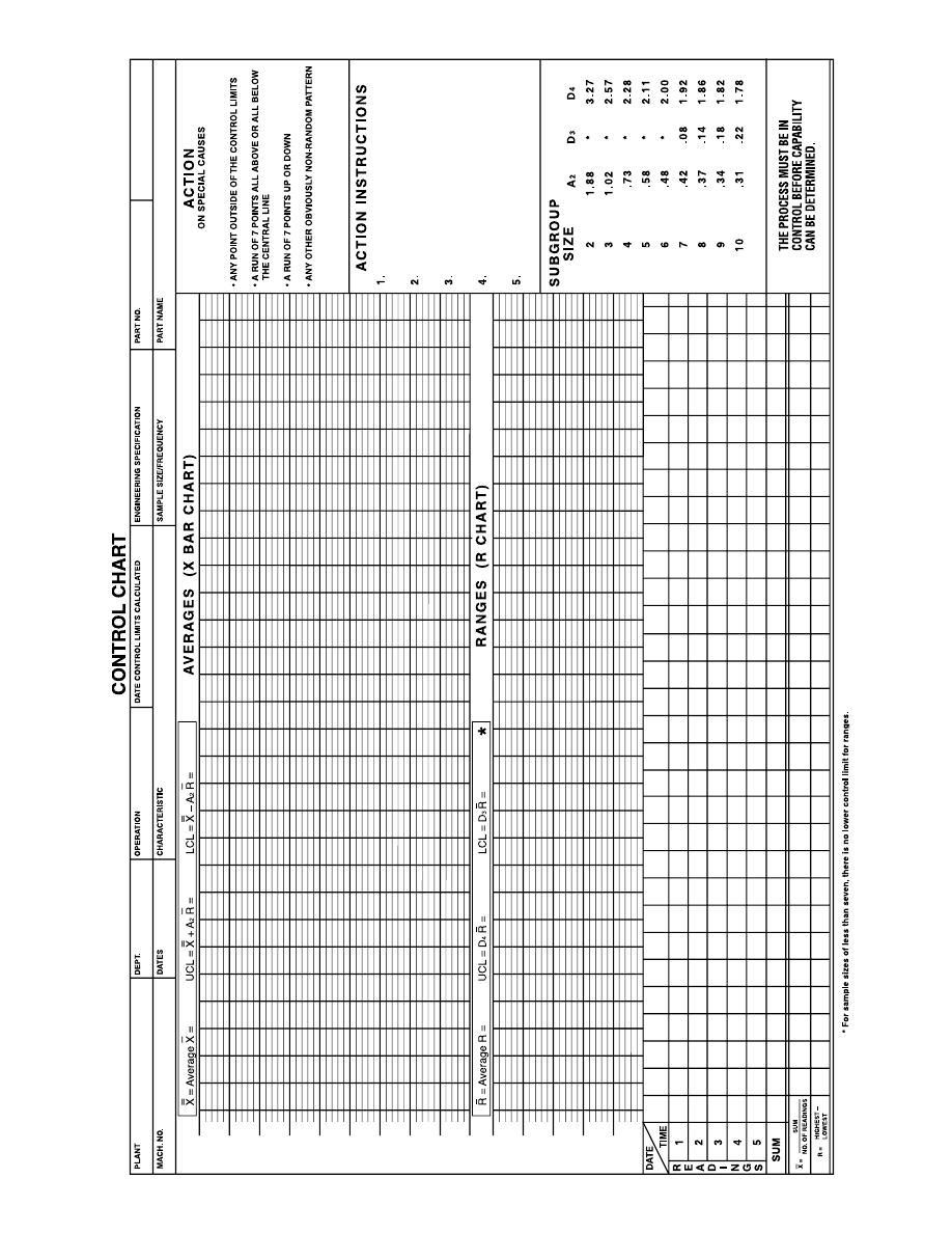
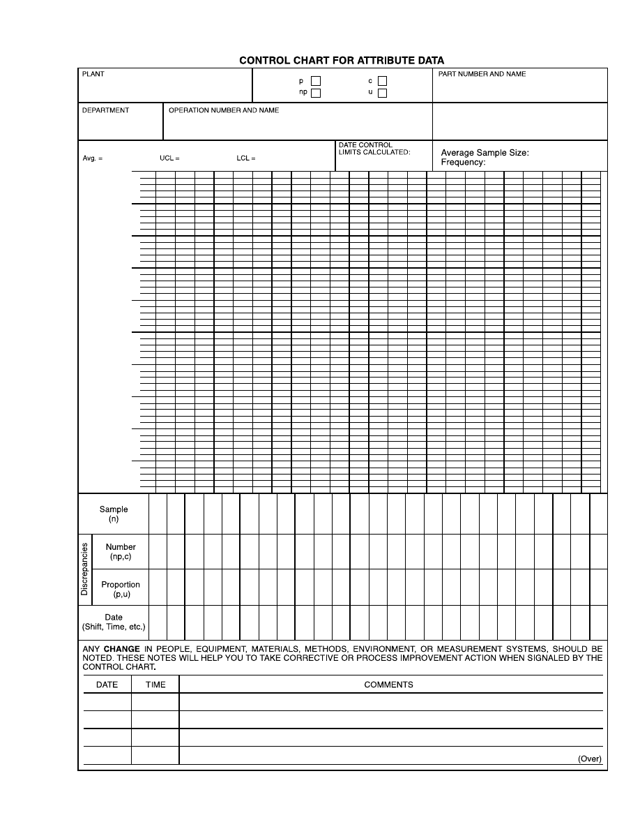
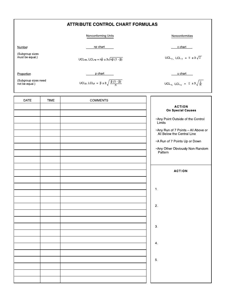
Supplier/SPC Manual User

Feedback Process

Consistent with the concept of continual improvement, this automotive industry statistical process
control (SPC) manual is being subjected to a formal annual review/revision process during the month of
October of each calendar year. In line with the concept of customer satisfaction, this annual review will
entail consideration of not only any applicable vehicle manufacturer requirement changes from year to
year but also of feedback from users of the manual for the purpose of making it more value-added and
effective to the automotive industry and user communities. Accordingly, please feel free to offer, in
writing, your feedback comments, both pro and con, relative to the manual’s understandability, “user-
friendliness,” etc., in the area indicated below. Please indicate specific manual page numbers, where
appropriate. Forward your feedback to the address indicated below:

Your Name

Representing

Supplier/Company/Division Name

Address

Phone

( )

Please list your top three automotive customers and their locations.

Customer

Location

Customer

Location

Customer