
PyX Documentation
Release 0.11.1
Jörg Lehmann, Michael Schindler, André Wobst
2011/05/20


CONTENTS
3
Organisation of the PyX package
. . . . . . . . . . . . . . . . . . . . . . . . . . . . . . . . . .
3
5
. . . . . . . . . . . . . . . . . . . . . . . . . . . . . . . . . . . . . . . . . . . . .
5
. . . . . . . . . . . . . . . . . . . . . . . . . . . . . . . . . . . . . . . . . . . .
6
Attributes: Styles and Decorations
. . . . . . . . . . . . . . . . . . . . . . . . . . . . . . . . . .
8
11
Class path — PostScript-like paths
. . . . . . . . . . . . . . . . . . . . . . . . . . . . . . . . .
11
. . . . . . . . . . . . . . . . . . . . . . . . . . . . . . . . . . . . . . . . . . . . .
12
. . . . . . . . . . . . . . . . . . . . . . . . . . . . . . . . . . . . . . . . . .
14
. . . . . . . . . . . . . . . . . . . . . . . . . . . . . . . . . . . . . . . .
14
. . . . . . . . . . . . . . . . . . . . . . . . . . . . . . . . . . . . . . . . . . .
15
Module deformer: Path deformers
17
19
. . . . . . . . . . . . . . . . . . . . . . . . . . . . . . . . . . . . . . . . . . . . .
19
21
. . . . . . . . . . . . . . . . . . . . . . . . . . . . . . . . . . . . . . . . . . . . . .
21
. . . . . . . . . . . . . . . . . . . . . . . . . . . . . . . . . . . . . . . . . .
21
. . . . . . . . . . . . . . . . . . . . . . . . . . . . . . . . . . . . . . . .
22
Module text: TeX/LaTeX interface
23
. . . . . . . . . . . . . . . . . . . . . . . . . . . . . . . . . . . . . . . . . .
23
TeX/LaTeX instances: the texrunner class
. . . . . . . . . . . . . . . . . . . . . . . . . . . .
23
. . . . . . . . . . . . . . . . . . . . . . . . . . . . . . . . . . . . . . . .
25
Using the graphics-bundle with LaTeX
. . . . . . . . . . . . . . . . . . . . . . . . . . . . . . .
28
. . . . . . . . . . . . . . . . . . . . . . . . . . . . . . . . . . . . . . . . .
28
. . . . . . . . . . . . . . . . . . . . . . . . . . . . . . . .
29
Some internals on temporary files etc.
. . . . . . . . . . . . . . . . . . . . . . . . . . . . . . . .
29
31
. . . . . . . . . . . . . . . . . . . . . . . . . . . . . . . . . . . . . . . . . . . . .
31
. . . . . . . . . . . . . . . . . . . . . . . . . . . . . . . . . . . . . . .
32
Module graph.graph: Graph geometry
. . . . . . . . . . . . . . . . . . . . . . . . . . . . .
33
. . . . . . . . . . . . . . . . . . . . . . . . . . . . . . . . .
36
Module graph.style: Graph styles
. . . . . . . . . . . . . . . . . . . . . . . . . . . . . . .
39
. . . . . . . . . . . . . . . . . . . . . . . . . . . . . . . . .
43
45
. . . . . . . . . . . . . . . . . . . . . . . . . . . . . . . . . . . . . . .
45
i

. . . . . . . . . . . . . . . . . . . . . . . . . . . . . . . .
45
Module graph.axis.tick: Axes ticks
. . . . . . . . . . . . . . . . . . . . . . . . . . . . .
48
Module graph.axis.parter: Axes partitioners
. . . . . . . . . . . . . . . . . . . . . . . .
49
Module graph.axis.texter: Axes texter
. . . . . . . . . . . . . . . . . . . . . . . . . . .
50
Module graph.axis.painter: Axes painter
. . . . . . . . . . . . . . . . . . . . . . . . . .
52
Module graph.axis.rater: Axes rater
. . . . . . . . . . . . . . . . . . . . . . . . . . . .
53
Module graph.axis.positioner: Axes positioners
. . . . . . . . . . . . . . . . . . . . .
54
10 Module box: Convex box handling
57
. . . . . . . . . . . . . . . . . . . . . . . . . . . . . . . . . . . . . . . . . . . . . . . .
57
10.2 Functions working on a box list
. . . . . . . . . . . . . . . . . . . . . . . . . . . . . . . . . . .
58
. . . . . . . . . . . . . . . . . . . . . . . . . . . . . . . . . . . . . . . . . .
58
59
. . . . . . . . . . . . . . . . . . . . . . . . . . . . . . . . . . . . . . . . . . . . . .
59
. . . . . . . . . . . . . . . . . . . . . . . . . . . . . . . . . . . . . . . . . . . . . .
59
. . . . . . . . . . . . . . . . . . . . . . . . . . . . . . . . . . . . . . . . . . . . .
59
. . . . . . . . . . . . . . . . . . . . . . . . . . . . . . . . . . . . . . . . . .
60
12 Module epsfile: EPS file inclusion
61
63
. . . . . . . . . . . . . . . . . . . . . . . . . . . . . . . . . . . . . . . . . . . . .
63
13.2 Bitmap module: Bitmap support
. . . . . . . . . . . . . . . . . . . . . . . . . . . . . . . . . .
64
65
. . . . . . . . . . . . . . . . . . . . . . . . . . . . . . . . . . . . . . . . . . .
65
. . . . . . . . . . . . . . . . . . . . . . . . . . . . . . . . . . . . . . . . . . . . .
65
67
. . . . . . . . . . . . . . . . . . . . . . . . . . . . . . . . . . . . . . . . . . . . .
67
. . . . . . . . . . . . . . . . . . . . . . . . . . . . . . . . . . . . . . . . . . . . . . .
67
. . . . . . . . . . . . . . . . . . . . . . . . . . . . . . . . . . . . . . . . . . . .
67
. . . . . . . . . . . . . . . . . . . . . . . . . . . . . . . . . . . . . . . . . . . . .
68
69
. . . . . . . . . . . . . . . . . . . . . . . . . . . . . . . . . . . . . . . . . . .
69
71
. . . . . . . . . . . . . . . . . . . . . . . . . . . . . . . . . . . . . . . . . . . . .
71
17.2 Predefined length instances
. . . . . . . . . . . . . . . . . . . . . . . . . . . . . . . . . . . . .
72
. . . . . . . . . . . . . . . . . . . . . . . . . . . . . . . . . . . . . . . . .
72
18 Module trafo: Linear transformations
73
. . . . . . . . . . . . . . . . . . . . . . . . . . . . . . . . . . . . . . . . . . . . . .
73
. . . . . . . . . . . . . . . . . . . . . . . . . . . . . . . . . . . . . . . . . .
74
75
77
79
22 Appendix: Arrows in deco module
81
83
85
ii

PyX Documentation, Release 0.11.1
Abstract
PyX is a Python package for the creation of PostScript and PDF files. It combines an abstraction of the
PostScript drawing model with a TeX/LaTeX interface. Complex tasks like 2d and 3d plots in publication-
ready quality are built out of these primitives.
CONTENTS
1

PyX Documentation, Release 0.11.1
2
CONTENTS

CHAPTER
ONE
INTRODUCTION
PyX is a Python package for the creation of vector graphics. As such it readily allows one to generate encap-
sulated PostScript files by providing an abstraction of the PostScript graphics model. Based on this layer and in
combination with the full power of the Python language itself, the user can just code any complexity of the figure
wanted. PyX distinguishes itself from other similar solutions by its TeX/LaTeX interface that enables one to make
direct use of the famous high quality typesetting of these programs.
A major part of PyX on top of the already described basis is the provision of high level functionality for complex
tasks like 2d plots in publication-ready quality.
1.1 Organisation of the PyX package
The PyX package is split in several modules, which can be categorised in the following groups
Functionality
Modules
basic graphics functionality
, deco,
, and
text output via TeX/LaTeX
and
linear transformations and units
and
graph plotting functionality
(including submodules) and
(including submodules)
EPS file inclusion
These modules (and some other less import ones) are imported into the module namespace by using
from
pyx
import
*
at the beginning of the Python program. However, in order to prevent namespace pollution, you may also simply
use import pyx. Throughout this manual, we shall always assume the presence of the above given import line.a
3

PyX Documentation, Release 0.11.1
4
Chapter 1. Introduction

CHAPTER
TWO
BASIC GRAPHICS
2.1 Introduction
The path module allows one to construct PostScript-like paths, which are one of the main building blocks for the
generation of drawings. A PostScript path is an arbitrary shape consisting of straight lines, arc segments and cubic
Bézier curves. Such a path does not have to be connected but may also comprise several disconnected segments,
which will be called subpaths in the following.
XXX example for paths and subpaths (figure)
Usually, a path is constructed by passing a list of the path primitives moveto, lineto, curveto, etc., to the
constructor of the
class. The following code snippet, for instance, defines a path p that consists of a straight
line from the point
(0, 0) to the point (1, 1)
from
pyx
import
*
p
=
path
.
path(path
.
moveto(
0
,
0
), path
.
lineto(
1
,
1
))
Equivalently, one can also use the predefined
subclass line and write
p
=
path
.
line(
0
,
0
,
1
,
1
)
While already some geometrical operations can be performed with this path (see next section), another PyX object
is needed in order to actually being able to draw the path, namely an instance of the
class. By convention,
we use the name c for this instance:
c
=
canvas
.
canvas()
In order to draw the path on the canvas, we use the stroke() method of the
class, i.e.,
c
.
stroke(p)
c
.
writeEPSfile(
"line"
)
To complete the example, we have added a writeEPSfile() call, which writes the contents of the canvas
to the file line.eps. Note that an extension .eps is added automatically, if not already present in the given
filename. Similarly, if you want to generate a PDF file instead, use
c
.
writePDFfile(
"line"
)
As a second example, let us define a path which consists of more than one subpath:
cross
=
path
.
path(path
.
moveto(
0
,
0
), path
.
rlineto(
1
,
1
),
path
.
moveto(
1
,
0
), path
.
rlineto(
-
1
,
1
))
The first subpath is again a straight line from
(0, 0) to (1, 1), with the only difference that we now have used the
rlineto
class, whose arguments count relative from the last point in the path. The second moveto instance
opens a new subpath starting at the point
(1, 0) and ending at (0, 1). Note that although both lines intersect at
the point
(1/2, 1/2), they count as disconnected subpaths. The general rule is that each occurrence of a moveto
instance opens a new subpath. This means that if one wants to draw a rectangle, one should not use
5

PyX Documentation, Release 0.11.1
rect1
=
path
.
path(path
.
moveto(
0
,
0
), path
.
lineto(
0
,
1
),
path
.
moveto(
0
,
1
), path
.
lineto(
1
,
1
),
path
.
moveto(
1
,
1
), path
.
lineto(
1
,
0
),
path
.
moveto(
1
,
0
), path
.
lineto(
0
,
0
))
which would construct a rectangle out of four disconnected subpaths (see Fig.
a). In a better
solution (see Fig.
b), the pen is not lifted between the first and the last point:
(a)
(b)
(c)
(d)
Figure 2.1: Rectangle example
Rectangle consisting of (a) four separate lines, (b) one open path, and (c) one closed path. (d) Filling a path always closes it
automatically.
rect2
=
path
.
path(path
.
moveto(
0
,
0
), path
.
lineto(
0
,
1
),
path
.
lineto(
1
,
1
), path
.
lineto(
1
,
0
),
path
.
lineto(
0
,
0
))
However, as one can see in the lower left corner of Fig.
b, the rectangle is still incomplete. It
needs to be closed, which can be done explicitly by using for the last straight line of the rectangle (from the point
(0, 1) back to the origin at (0, 0)) the closepath directive:
rect3
=
path
.
path(path
.
moveto(
0
,
0
), path
.
lineto(
0
,
1
),
path
.
lineto(
1
,
1
), path
.
lineto(
1
,
0
),
path
.
closepath())
The closepath directive adds a straight line from the current point to the first point of the current subpath
and furthermore closes the sub path, i.e., it joins the beginning and the end of the line segment. This results in
the intended rectangle shown in Fig.
c. Note that filling the path implicitly closes every open
subpath, as is shown for a single subpath in Fig.
d), which results from
c
.
stroke(rect2, [deco
.
filled([color
.
grey(
0.95
)])])
Here, we supply as second argument of the stroke() method a list which in the present case only consists
of a single element, namely the so called decorator deco.filled. As it name says, this decorator specifies
that the path is not only being stroked but also filled with the given color. More information about decorators,
styles and other attributes which can be passed as elements of the list can be found in Sect.
. More details on the available path elements can be found in Sect.
To conclude this section, we should not forget to mention that rectangles are, of course, predefined in PyX, so
above we could have as well written
rect2
=
path
.
rect(
0
,
0
,
1
,
1
)
Here, the first two arguments specify the origin of the rectangle while the second two arguments define its width
and height, respectively. For more details on the predefined paths, we refer the reader to Sect.
2.2 Path operations
Often, one wants to perform geometrical operations with a path before placing it on a canvas by stroking or filling
it. For instance, one might want to intersect one path with another one, split the paths at the intersection points,
and then join the segments together in a new way. PyX supports such tasks by means of a number of path methods,
which we will introduce in the following.
6
Chapter 2. Basic graphics
PyX Documentation, Release 0.11.1
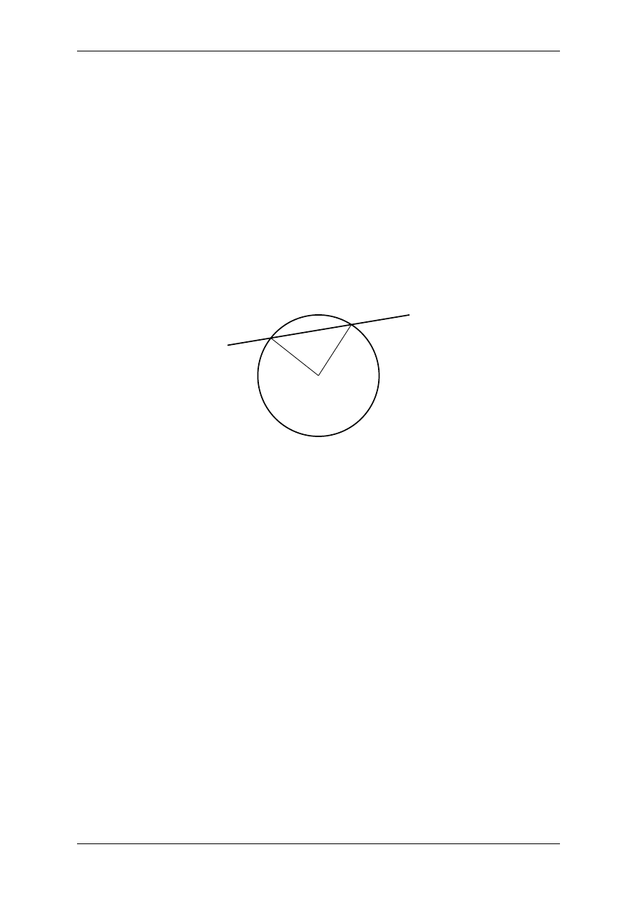
Suppose you want to draw the radii to the intersection points of a circle with a straight line. This task can be done
using the following code which results in Fig.
Example: Intersection of circle with line yielding two radii.
from
pyx
import
*
c
=
canvas
.
canvas()
circle
=
path
.
circle(
0
,
0
,
2
)
line
=
path
.
line(
-
3
,
1
,
3
,
2
)
c
.
stroke(circle, [style
.
linewidth
.
Thick])
c
.
stroke(line, [style
.
linewidth
.
Thick])
isects_circle, isects_line
=
circle
.
intersect(line)
for
isect
in
isects_circle:
isectx, isecty
=
circle
.
at(isect)
c
.
stroke(path
.
line(
0
,
0
, isectx, isecty))
c
.
writeEPSfile(
"radii"
)
c
.
writePDFfile(
"radii"
)
Figure 2.2: Example: Intersection of circle with line yielding two radii.
Here, the basic elements, a circle around the point
(0, 0) with radius 2 and a straight line, are defined. Then,
passing the line, to the intersect() method of circle, we obtain a tuple of parameter values of the intersection
points. The first element of the tuple is a list of parameter values for the path whose intersect() method has
been called, the second element is the corresponding list for the path passed as argument to this method. In the
present example, we only need one list of parameter values, namely isects_circle. Using the at() path method
to obtain the point corresponding to the parameter value, we draw the radii for the different intersection points.
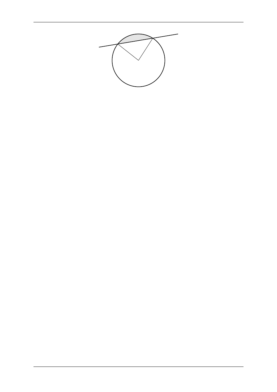
Another powerful feature of PyX is its ability to split paths at a given set of parameters. For instance, in order to
fill in the previous example the segment of the circle delimited by the straight line (cf. Fig.
of circle with line yielding radii and circle segment.
), one first has to construct a path corresponding to the outline
of this segment. The following code snippet yields this segment
arc1, arc2
=
circle
.
split(isects_circle)
if
arc1
.
arclen()
<
arc2
.
arclen():
arc
=
arc1
else
:
arc
=
arc2
isects_line
.
sort()
line1, line2, line3
=
line
.
split(isects_line)
segment
=
line2
<<
arc
Here, we first split the circle using the split() method passing the list of parameters obtained above. Since the
circle is closed, this yields two arc segments. We then use the arclen(), which returns the arc length of the
path, to find the shorter of the two arcs. Before splitting the line, we have to take into account that the split()
method only accepts a sorted list of parameters. Finally, we join the straight line and the arc segment. For this,
we make use of the << operator, which not only adds the paths (which could be done using line2 + arc), but
also joins the last subpath of line2 and the first one of arc. Thus, segment consists of only a single subpath and
2.2. Path operations
7
PyX Documentation, Release 0.11.1
Figure 2.3: Example: Intersection of circle with line yielding radii and circle segment.
filling works as expected.
An important issue when operating on paths is the parametrisation used. Internally, PyX uses a parametrisation
which uses an interval of length
1 for each path element of a path. For instance, for a simple straight line, the
possible parameter values range from
0 to 1, corresponding to the first and last point, respectively, of the line.
Appending another straight line, would extend this range to a maximal value of
2.
However, the situation becomes more complicated if more complex objects like a circle are involved. Then, one
could be tempted to assume that again the parameter value ranges from
0 to 1, because the predefined circle
consists just of one arc together with a closepath element. However, this is not the case: the actual range
is much larger. The reason for this behaviour lies in the internal path handling of PyX: Before performing any
non-trivial geometrical operation with a path, it will automatically be converted into an instance of the normpath
class (see also Sect.
). These so generated paths are already separated in their subpaths and
only contain straight lines and Bézier curve segments. Thus, as is easily imaginable, they are much simpler to deal
with.
XXX explain normpathparams and things like p.begin(), p.end()-1,
A more geometrical way of accessing a point on the path is to use the arc length of the path segment from the first
point of the path to the given point. Thus, all PyX path methods that accept a parameter value also allow the user
to pass an arc length. For instance,
from
math
import
pi
r
=
2
pt1
=
path
.
circle(
0
,
0
, r)
.
at(r
*
pi)
pt2
=
path
.
circle(
0
,
0
, r)
.
at(r
*
3
*
pi
/
2
)
c
.
stroke(path
.
path(path
.
moveto(
*
pt1), path
.
lineto(
*
pt2)))
will draw a straight line from a point at angle
180 degrees (in radians π) to another point at angle 270 degrees
(in radians
3π/2) on a circle with radius r = 2. Note however, that the mapping arc length → point is in general
discontinuous at the begin and the end of a subpath, and thus PyX does not guarantee any particular result for this
boundary case.
More information on the available path methods can be found in Sect.
2.3 Attributes: Styles and Decorations
Attributes define properties of a given object when it is being used. Typically, there are different kind of attributes
which are usually orthogonal to each other, while for one type of attribute, several choices are possible. An
example is the stroking of a path. There, linewidth and linestyle are different kind of attributes. The linewidth
might be normal, thin, thick, etc, and the linestyle might be solid, dashed etc.
Attributes always occur in lists passed as an optional keyword argument to a method or a function. Usually,
attributes are the first keyword argument, so one can just pass the list without specifying the keyword. Again, for
the path example, a typical call looks like
8
Chapter 2. Basic graphics

PyX Documentation, Release 0.11.1
c
.
stroke(path, [style
.
linewidth
.
Thick, style
.
linestyle
.
dashed])
Here, we also encounter another feature of PyX’s attribute system. For many attributes useful default values are
stored as member variables of the actual attribute. For instance, style.linewidth.Thick is equivalent to
style.linewidth(0.04, type="w", unit="cm")
, that is
0.04 width cm (see Sect.
for more
information about PyX’s unit system).
Another important feature of PyX attributes is what is call attributed merging. A trivial example is the following:
# the following two lines are equivalent
c
.
stroke(path, [style
.
linewidth
.
Thick, style
.
linewidth
.
thin])
c
.
stroke(path, [style
.
linewidth
.
thin])
Here, the style.linewidth.thin attribute overrides the preceding style.linewidth.Thick decla-
ration. This is especially important in more complex cases where PyXdefines default attributes for a certain
operation. When calling the corresponding methods with an attribute list, this list is appended to the list of de-
faults. This way, the user can easily override certain defaults, while leaving the other default values intact. In
addition, every attribute kind defines a special clear attribute, which allows to selectively delete a default value.
For path stroking this looks like
# the following two lines are equivalent
c
.
stroke(path, [style
.
linewidth
.
Thick, style
.
linewidth
.
clear])
c
.
stroke(path)
The clear attribute is also provided by the base classes of the various styles.
For instance,
style.strokestyle.clear
clears all strokestyle subclasses and thus style.linewidth and
style.linestyle
.
Since all attributes derive from attr.attr, you can remove all defaults using
attr.clear
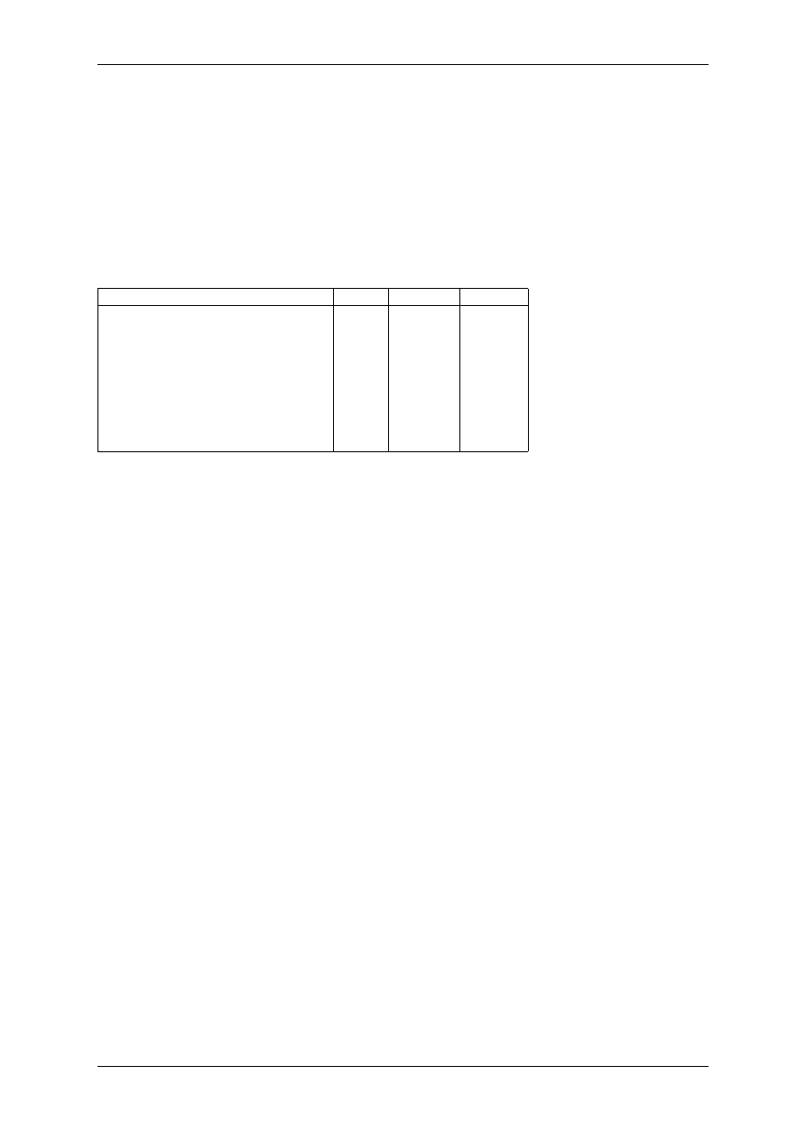
. An overview over the most important attribute typesprovided by PyX is given in the following
table.
Attribute
category
description
examples
deco.deco
decorator specifying
the way the path is
drawn
deco.stroked
, deco.filled, deco.arrow
style.strokestyle
style used for path
stroking
style.linecap
, style.linejoin, style.miterlimit,
style.dash
, style.linestyle, style.linewidth,
color.color
style.fillstyle
style used for path
filling
color.color
, pattern.pattern
style.filltype
type of path filling
style.filltype.nonzero_winding
(default),
style.filltype.even_odd
operations changing
the shape of the path
text.textattr
attributes used for
typesetting
trafo.trafo
ransformations
applied when
drawing object
trafo.mirror
, trafo.rotate, trafo.scale,
trafo.slant
, trafo.translate
XXX specify which classes in the table are in fact instances
Note that operations usually allow for certain attribute categories only. For example when stroking a path, text
attributes are not allowed, while stroke attributes and decorators are. Some attributes might belong to several
attribute categories like colours, which are both, stroke and fill attributes.
Last, we discuss another important feature of PyX’s attribute system. In order to allow the easy customisation
of predefined attributes, it is possible to create a modified attribute by calling of an attribute instance, thereby
specifying new parameters. A typical example is to modify the way a path is stroked or filled by constructing
appropriate deco.stroked or deco.filled instances. For instance, the code
2.3. Attributes: Styles and Decorations
9

PyX Documentation, Release 0.11.1
c
.
stroke(path, [deco
.
filled([color
.
rgb
.
green])])
draws a path filled in green with a black outline. Here, deco.filled is already an instance which is modified
to fill with the given color. Note that an equivalent version would be
c
.
draw(path, [deco
.
stroked, deco
.
filled([color
.
rgb
.
green])])
In particular, you can see that deco.stroked is already an attribute instance, since otherwise you were not
allowed to pass it as a parameter to the draw method. Another example where the modification of a decorator is
useful are arrows. For instance, the following code draws an arrow head with a more acute angle (compared to the
default value of
45 degrees):
c
.
stroke(path, [deco
.
earrow(angle
=
30
)])
XXX changeable attributes
10
Chapter 2. Basic graphics

CHAPTER
THREE
MODULE PATH
The
module defines several important classes which are documented in the present section.
3.1 Class path — PostScript-like paths
class path.path(*pathitems)
This class represents a PostScript like path consisting of the path elements pathitems.
All possible path items are described in Sect.
. Note that there are restrictions on the first path
element and likewise on each path element after a
directive. In both cases, no current point
is defined and the path element has to be an instance of one of the following classes:
, and
Instances of the class
provide the following methods (in alphabetic order):
path.append(
pathitem)
Appends a pathitem to the end of the path.
path.arclen()
Returns the total arc length of the path.
†
path.arclentoparam(
lengths)
Returns the parameter value(s) corresponding to the arc length(s) lengths.
†
path.at(
params)
Returns the coordinates (as 2-tuple) of the path point(s) corresponding to the parameter value(s) params.
‡ †
path.atbegin()
Returns the coordinates (as 2-tuple) of the first point of the path.
†
path.atend()
Returns the coordinates (as 2-tuple) of the end point of the path.
†
path.bbox()
Returns the bounding box of the path. Note that this returned bounding box may be too large, if the path
contains any
elements, since for these the control box, i.e., the bounding box enclosing the
control points of the Bézier curve is returned.
path.begin()
Returns the parameter value (a normpathparam instance) of the first point in the path.
path.curveradius(
param=None
, arclen=None)
Returns the curvature radius/radii (or None if infinite) at parameter value(s) params.
‡
This is the inverse of
the curvature at this parameter. Note that this radius can be negative or positive, depending on the sign of
the curvature.
†
path.end()
Returns the parameter value (a normpathparam instance) of the last point in the path.
11

PyX Documentation, Release 0.11.1
path.extend(
pathitems)
Appends the list pathitems to the end of the path.
path.intersect(
opath)
Returns a tuple consisting of two lists of parameter values corresponding to the intersection points of the
path with the other path opath, respectively.
†
For intersection points which are not farther apart then epsilon
points, only one is returned.
path.joined(
opath)
Appends opath to the end of the path, thereby merging the last subpath (which must not be closed) of the
path with the first sub path of opath and returns the resulting new path.
†
path.normpath(
epsilon=None)
Returns the equivalent
. For the conversion and for later calculations with this
and
accuracy of epsilon points is used. If epsilon is None, the global epsilon of the
module is used.
path.paramtoarclen(
params)
Returns the arc length(s) corresponding to the parameter value(s) params.
‡ †
path.range()
Returns the maximal parameter value param that is allowed in the path methods.
path.reversed()
Returns the reversed path.
†
path.rotation(
params)
Returns (a) rotations(s) which (each), which rotate the x-direction to the tangent and the y-direction to the
normal at that param.
†
path.split(
params)
Splits the path at the parameter values params, which have to be sorted in ascending order, and returns a
corresponding list of
instances.
†
path.tangent(
params
, length=1)
Return (a)
instance(s) corresponding to the tangent vector(s) to the path at the parameter value(s)
params
.
‡
The tangent vector will be scaled to the length length.
†
path.trafo(
params)
Returns (a) trafo(s) which (each) translate to a point on the path corresponding to the param, rotate the
x-direction to the tangent and the y-direction to the normal in that point.
†
path.transformed(
trafo)
Returns the path transformed according to the linear transformation trafo. Here, trafo must be an instance
of the trafo.trafo class.
†
Some notes on the above:
• The
† denotes methods which require a prior conversion of the path into a
instance. This is
done automatically (using the precision epsilon set globally using path.set()). If you need a different
epsilon
for a normpath, you also can perform the conversion manually.
• Instead of using the joined() method, you can also join two paths together with help of the << operator,
for instance p = p1 << p2.
•
‡
In these methods, params may either be a single value or a list. In the latter case, the result of the method
will be a list consisting of the results for every parameter. The parameter itself may either be a length (or
a number which is then interpreted as a user length) or an instance of the class normpathparam. In the
former case, the length refers to the arc length along the path.
3.2 Path elements
The class pathitem is the superclass of all PostScript path construction primitives. It is never used directly, but
only by instantiating its subclasses, which correspond one by one to the PostScript primitives.
12
Chapter 3. Module path

PyX Documentation, Release 0.11.1
Except for the path elements ending in _pt, all coordinates passed to the path elements can be given as number
(in which case they are interpreted as user units with the currently set default type) or in PyX lengths.
The following operation move the current point and open a new subpath:
class path.moveto(x, y)
Path element which sets the current point to the absolute coordinates (x, y). This operation opens a new
subpath.
class path.rmoveto(dx, dy)
Path element which moves the current point by (dx, dy). This operation opens a new subpath.
Drawing a straight line can be accomplished using:
class path.lineto(x, y)
Path element which appends a straight line from the current point to the point with absolute coordinates (x,
y
), which becomes the new current point.
class path.rlineto(dx, dy)
Path element which appends a straight line from the current point to the a point with relative coordinates
(dx, dy), which becomes the new current point.
For the construction of arc segments, the following three operations are available:
class path.arc(x, y, r, angle1, angle2)
Path element which appends an arc segment in counterclockwise direction with absolute coordinates (x, y)
of the center and radius r from angle1 to angle2 (in degrees). If before the operation, the current point is
defined, a straight line is from the current point to the beginning of the arc segment is prepended. Otherwise,
a subpath, which thus is the first one in the path, is opened. After the operation, the current point is at the
end of the arc segment.
class path.arcn(x, y, r, angle1, angle2)
Path element which appends an arc segment in clockwise direction with absolute coordinates (x, y) of the
center and radius r from angle1 to angle2 (in degrees). If before the operation, the current point is defined,
a straight line is from the current point to the beginning of the arc segment is prepended. Otherwise, a
subpath, which thus is the first one in the path, is opened. After the operation, the current point is at the end
of the arc segment.
class path.arct(x1, y1, x2, y2, r)
Path element which appends an arc segment of radius r connecting between (x1, y1) and (x2, y2). —
Bézier curves can be constructed using:
class path.curveto(x1, y1, x2, y2, x3, y3)
Path element which appends a Bézier curve with the current point as first control point and the other control
points (x1, y1), (x2, y2), and (x3, y3).
class path.rcurveto(dx1, dy1, dx2, dy2, dx3, dy3)
Path element which appends a Bézier curve with the current point as first control point and the other control
points defined relative to the current point by the coordinates (dx1, dy1), (dx2, dy2), and (dx3, dy3).
Note that when calculating the bounding box (see Sect.
) of Bézier curves, PyX uses for performance
reasons the so-called control box, i.e., the smallest rectangle enclosing the four control points of the Bézier curve.
In general, this is not the smallest rectangle enclosing the Bézier curve.
Finally, an open subpath can be closed using:
class path.closepath
Path element which closes the current subpath.
For performance reasons, two non-PostScript path elements are defined, which perform multiple identical opera-
tions:
class path.multilineto_pt(points_pt)
Path element which appends straight line segments starting from the current point and going through the list
of points given in the points_pt argument. All coordinates have to be given in PostScript points.
3.2. Path elements
13

PyX Documentation, Release 0.11.1
class path.multicurveto_pt(points_pt)
Path element which appends Bézier curve segments starting from the current point and going through the
list of each three control points given in the points_pt argument. Thus, points_pt must be a sequence of
6-tuples.
3.3 Class normpath
The
class is used internally for all non-trivial path operations, i.e. the ones marked by a
† in the
description of the
above. It represents a path as a list of subpaths, which are instances of the class
. These
s themselves consist of a list of normsubpathitems which are ei-
ther straight lines (normline) or Bézier curves (normcurve).
A given path can easily be converted to the corresponding
using the method with this name:
np
=
p
.
normpath()
Additionally, you can specify the accuracy (in points) which is used in all
calculations by means of the
argument epsilon, which defaults to to
10
−5
points. This default value can be changed using the module function
path.set()
.
To construct a
from a list of
instances, you pass them to the
constructor:
class path.normpath(normsubpaths=
[ ]
)
Construct a
consisting of subnormpaths, which is a list of subnormpath instances.
Instances of
offers all methods of regular
s, which also have the same semantics. An exception
are the methods append() and extend(). While they allow for adding of instances of subnormpath to the
instance, they also keep the functionality of a regular path and allow for regular path elements to be
appended. The later are converted to the proper normpath representation during addition.
In addition to the
methods, a
instance also offers the following methods, which operate on the
instance itself, i.e., modify it in place.
normpath.join(
other)
Join other, which has to be a
instance, to the
instance.
normpath.reverse()
Reverses the
instance.
normpath.transform(
trafo)
Transforms the
instance according to the linear transformation trafo.
Finally, we remark that the sum of a
and a
always yields a
3.4 Class normsubpath
class path.normsubpath(normsubpathitems=
[ ]
, closed=0, epsilon=1e-5)
Construct a
consisting of normsubpathitems, which is a list of normsubpathitem in-
stances. If closed is set, the
will be closed, thereby appending a straight line segment from
the first to the last point, if it is not already present. All calculations with the
are performed
with an accuracy of epsilon.
Most
methods behave like the ones of a
Exceptions are:
normsubpath.append(
anormsubpathitem)
Append the anormsubpathitem to the end of the
instance. This is only possible if the
is not closed, otherwise an exception is raised.
14
Chapter 3. Module path

PyX Documentation, Release 0.11.1
normsubpath.extend(
normsubpathitems)
Extend the
instances by normsubpathitems, which has to be a list of normsubpathitem
instances. This is only possible if the
is not closed, otherwise an exception is raised.
normsubpath.close()
Close the
instance, thereby appending a straight line segment from the first to the last point,
if it is not already present.
3.5 Predefined paths
For convenience, some oft-used paths are already predefined. All of them are subclasses of the
class.
class path.line(x0, y0, x1, y1)
A straight line from the point (x0, y0) to the point (x1, y1).
class path.curve(x0, y0, x1, y1, x2, y2, x3, y3)
A Bézier curve with control points (x0, y0),
. . . , (x3, y3).
class path.rect(x, y, w, h)
A closed rectangle with lower left point (x, y), width w, and height h.
class path.circle(x, y, r)
A closed circle with center (x, y) and radius r.
3.5. Predefined paths
15

PyX Documentation, Release 0.11.1
16
Chapter 3. Module path

CHAPTER
FOUR
MODULE DEFORMER: PATH
DEFORMERS
The
module provides techniques to generate modulated paths. All classes in the
module
can be used as attributes when drawing/stroking paths onto a canvas, but also independently for manipulating
previously created paths. The difference to the classes in the deco module is that here, a totally new path is
constructed.
All classes of the
module provide the following methods:
class deformer.deformer
deformer.__call__(
(specific parameters for the class))
Returns a deformer with modified parameters
deformer.deform(
path)
Returns the deformed normpath on the basis of the path. This method allows using the deformers outside
of a drawing call.
The deformer classes are the following:
class deformer.cycloid(radius, halfloops=10, skipfirst=1*unit.t_cm, skiplast=1*unit.t_cm, curves-
perhloop=3
, sign=1, turnangle=45)
This deformer creates a cycloid around a path. The outcome looks similar to a 3D spring stretched along
the original path.
radius
: the radius of the cycloid (this is the radius of the 3D spring)
halfloops
: the number of half-loops of the cycloid
skipfirst
and skiplast: the lengths on the original path not to be bent to a cycloid
curvesperhloop
: the number of Bezier curves to approximate a half-loop
sign
: with sign>=0 starts the cycloid to the left of the path, sign<0 to the right.
turnangle
: the angle of perspective on the 3D spring. At turnangle=0 one sees a sinusoidal curve, at
turnangle=90
one essentially sees a circle.
class deformer.smoothed(radius, softness=1, obeycurv=0, relskipthres=0.01)
This deformer creates a smoothed variant of the original path. The smoothing is done on the basis of the
corners of the original path, not on a global skope! Therefore, the result might not be what one would draw
by hand. At each corner (or wherever two path elements meet) a piece of length
2× radius is taken out
of the original path and replaced by a curve. This curve is determined by the tangent directions and the
curvatures at its endpoints. Both are given from the original path, and therefore, the new curve fits into the
gap in a geometrically smooth way. Path elements that are shorter than radius
× relskipthres are ignored.
The new curve smoothing the corner consists either of one or of two Bezier curves, depending on the
surrounding path elements. If there are straight lines before and after the new curve, then two Bezier curves
are used. This optimises the bending of curves in rectangular boxes or polygons. Here, the curves have an
additional degree of freedom that can be set with softness
∈ (0, 1]. If one of the concerned path elements is
17

PyX Documentation, Release 0.11.1
curved, only one Bezier curve is used that is (not always uniquely) determined by its geometrical constraints.
There are, nevertheless, some caveats:
A curve that strictly obeys the sign and magnitude of the curvature might not look very smooth in some
cases. Especially when connecting a curved with a straight piece, the smoothed path contains unwanted
overshootings. To prevent this, the parameter default obeycurv=0 releases the curvature constraints a little:
The curvature may then change its sign (still looks smooth for human eyes) or, in more extreme cases, even
its magnitude (does not look so smooth). If you really need a geometrically smooth path on the basis of
Bezier curves, then set obeycurv=1.
class deformer.parallel(distance, relerr=0.05, sharpoutercorners=0, dointersection=1, checkdis-
tanceparams=[0.5], lookforcurvatures=11)
This deformer creates a parallel curve to a given path. The result is similar to what is usually referred to as
the set with constant distance to the set of points on the path. It differs in one important respect, because
the distance parameter in the deformer is a signed distance. The resulting parallel normpath is constructed
on the level of the original pathitems. For each of them a parallel pathitem is constructed. Then, they are
connected by circular arcs (or by sharp edges) around the corners of the original path. Later, everything that
is nearer to the original path than distance is cut away.
There are some caveats:
•When the original path is too curved then the parallel path would contain points with infinte curvature.
The resulting path stops at such points and leaves the too strongly curved piece out.
•When the original path contains self-intersection, then the resulting parallel path is not continuous in
the parameterisation of the original path. It may first take a piece that corresponds to “later” parameter
values and then continue with an “earlier” one. Please don’t get confused.
The parameters are the following:
distance
is the minimal (signed) distance between the original and the parallel paths.
relerr
is the allowed error in the distance is given by distance*relerr.
sharpoutercorners
connects the parallel pathitems by wegde build of straight lines, instead of taking circular
arcs. This preserves the angle of the original corners.
dointersection
is a boolean for performing the last step, the intersection step, in the path construction.
Setting this to 0 gives the full parallel path, which can be favourable for self-intersecting paths.
checkdistanceparams
is a list of parameter values in the interval (0,1) where the distance is checked on each
parallel pathitem
lookforcurvatures
is the number of points per normpathitem where its curvature is checked for critical values
18
Chapter 4. Module deformer: Path deformers

CHAPTER
FIVE
MODULE CANVAS
One of the central modules for the PostScript access in PyX is named canvas. Besides providing the class
canvas
, which presents a collection of visual elements like paths, other canvases, TeX or LaTeX elements, it
contains the class canvas.clip which allows clipping of the output.
A canvas may also be embedded in another one using its insert method. This may be useful when you want to
apply a transformation on a whole set of operations..
5.1 Class canvas
This is the basic class of the canvas module, which serves to collect various graphical and text elements you want
to write eventually to an (E)PS file.
class canvas.canvas(attrs=
[ ]
, texrunner=None)
Construct a new canvas, applying the given attrs, which can be instances of trafo.trafo,
canvas.clip
, style.strokestyle or style.fillstyle. The texrunner argument can be used
to specify the texrunner instance used for the
method of the canvas. If not specified, it defaults to
text.defaulttexrunner
.
Paths can be drawn on the canvas using one of the following methods:
canvas.draw(
path
, attrs)
Draws path on the canvas applying the given attrs.
canvas.fill(
path
, attrs=
[ ]
)
Fills the given path on the canvas applying the given attrs.
canvas.stroke(
path
, attrs=
[ ]
)
Strokes the given path on the canvas applying the given attrs.
Arbitrary allowed elements like other
instances can be inserted in the canvas using
canvas.insert(
item
, attrs=
[ ]
)
Inserts an instance of base.canvasitem into the canvas. If attrs are present, item is inserted into a new
instance with attrs as arguments passed to its constructor is created. Then this
instance is
inserted itself into the canvas.
Text output on the canvas is possible using
canvas.text(
x
, y, text, attrs=
[ ]
)
Inserts text
at position (x,
y
) into the canvas applying attrs.
This is a shortcut for
insert(texrunner.text(x, y, text, attrs))
).
The
class provides access to the total geometrical size of its element:
canvas.bbox()
Returns the bounding box enclosing all elements of the canvas.
A canvas also allows one to set its TeX runner:
19

PyX Documentation, Release 0.11.1
canvas.settexrunner(
texrunner)
Sets a new texrunner for the canvas.
The contents of the canvas can be written using the following two convenience methods, which wrap the canvas
into a single page document.
canvas.writeEPSfile(
file
, *args, **kwargs)
Writes the canvas to file using the EPS format. file either has to provide a write method or it is used as
a string containing the filename (the extension .eps is appended automatically, if it is not present). This
method constructs a single page document, passing args and kwargs to the
constructor
and the calls the
method of this
instance passing the file.
canvas.writePSfile(
file
, *args, **kwargs)
Similar to
but using the PS format.
canvas.writePDFfile(
file
, *args, **kwargs)
Similar to
but using the PDF format.
canvas.writetofile(
filename
, *args, **kwargs)
Determine the file type (EPS, PS, or PDF) from the file extension of filename and call the corresponding
write method with the given arguments arg and kwargs.
canvas.pipeGS(
filename=”-“
, device=None, resolution=100, gscommand=”gs”, gsoptions=”“, tex-
talphabits=4
, graphicsalphabits=4, ciecolor=False, input=”eps”, **kwargs)
This method pipes the content of a canvas to the ghostscript interpreter directly to generate other output
formats. At least filename or device must be set. filename specifies the name of the output file. No file
extension will be added to that name in any case. When no filename is specified, the output is written to
stdout. device specifies a ghostscript output device by a string. Depending on your ghostscript configuration
"png16"
, "png16m", "png256", "png48", "pngalpha", "pnggray", "pngmono", "jpeg",
and "jpeggray" might be available among others. See the output of gs --help and the ghostscript
documentation for more information. When filename is specified but the device is not set, "png16m" is
used when the filename ends in .png and "jpeg" is used when the filename ends in .jpg.
resolution
specifies the resolution in dpi (dots per inch). gscmd is the command to be used to invoke
ghostscript. gsoptions are an option string passed to the ghostscript interpreter. textalphabits are graphic-
salphabits
are conventient parameters to set the TextAlphaBits and GraphicsAlphaBits options
of ghostscript. You can skip the addition of those option by set their value to None. ciecolor adds the
-dUseCIEColor
flag to improve the CMYK to RGB color conversion. input can be either "eps" or
"pdf"
to select the input type to be passed to ghostscript (note slightly different features available in the
different input types).
kwargs
are passed to the
method (not counting the file parameter), which is used to
generate the input for ghostscript. By that you gain access to the
constructor arguments.
For more information about the possible arguments of the
constructor, we refer to Sect.
20
Chapter 5. Module canvas

CHAPTER
SIX
MODULE DOCUMENT
The document module contains two classes:
and
. A
consists of one or several
6.1 Class page
A
is a thin wrapper around a
, which defines some additional properties of the page.
class document.page(canvas, pagename=None, paperformat=None, rotated=0, centered=1, fitto-
size=0
, margin=1 * unit.t_cm, bboxenlarge=1 * unit.t_pt, bbox=None)
Construct a new
from the given
instance. A string pagename and the paperformat can be
defined. See below, for a list of known paper formats. If rotated is set, the output is rotated by 90 degrees on
the page. If centered is set, the output is centered on the given paperformat. If fittosize is set, the output is
scaled to fill the full page except for a given margin. Normally, the bounding box of the canvas is calculated
automatically from the bounding box of its elements. Alternatively, you may specify the bbox manually. In
any case, the bounding box is enlarged on all sides by bboxenlarge.
6.2 Class document
class document.document(pages=
[ ]
)
Construct a
consisting of a given list of pages.
A
can be written to a file using one of the following methods:
document.writeEPSfile(
file
,
title=None
,
strip_fonts=True
,
text_as_path=False
,
mesh_as_bitmap=False
, mesh_as_bitmap_resolution=300)
Write a single page
to an EPS file. title is used as the document title, strip_fonts enabled font
stripping (removal of unused glyphs), text_as_path converts all text to paths instead of using fonts in the
output, mesh_as_bitmap converts meshs (like 3d surface plots) to bitmaps (to reduce complexity in the
output) and mesh_as_bitmap_resolution is the resolution of this conversion in dots per inch.
document.writePSfile(
file
, writebbox=False, title=None, strip_fonts=True, text_as_path=False,
mesh_as_bitmap=False
, mesh_as_bitmap_resolution=300)
Write
to a PS file. writebbox add the page bounding boxes to the output. All other parameters
are identical to the
method.
document.writePDFfile(
file
,
title=None
,
author=None
,
subject=None
,
keywords=None
,
fullscreen=False
, writebbox=False, compress=True, compresslevel=6,
strip_fonts=True
,
text_as_path=False
,
mesh_as_bitmap=False
,
mesh_as_bitmap_resolution=300)
Write
to a PDF file. author, subject, and keywords are used for the document author, subject,
and keyword information, respectively. fullscreen enabled fullscreen mode when the document is opened,
writebbox
enables writing of the crop box to each page, compress enables output stream compression and
compresslevel
sets the compress level to be used (from 1 to 9). All other parameters are identical to the
21
PyX Documentation, Release 0.11.1
document.writetofile(
filename
, *args, **kwargs)
Determine the file type (EPS, PS, or PDF) from the file extension of filename and call the corresponding
write method with the given arguments arg and kwargs.
6.3 Class paperformat
class document.paperformat(width, height, name=None)
Define a
with the given width and height and the optional name.
Predefined paperformats are listed in the following table
instance
name
width
height
document.paperformat.A0
A0
840 mm
1188 mm
document.paperformat.A0b
910 mm
1370 mm
document.paperformat.A1
A1
594 mm
840 mm
document.paperformat.A2
A2
420 mm
594 mm
document.paperformat.A3
A3
297 mm
420 mm
document.paperformat.A4
A4
210 mm
297 mm
document.paperformat.A5
A5
148.5 mm
210 mm
document.paperformat.Letter
Letter
8.5 inch
11 inch
document.paperformat.Legal
Legal
8.5 inch
14 inch
22
Chapter 6. Module document

CHAPTER
SEVEN
MODULE TEXT: TEX/LATEX
INTERFACE
7.1 Basic functionality
The
module seamlessly integrates Donald E. Knuths famous TeX typesetting engine into PyX. The basic
procedure is:
• start a TeX/LaTeX instance as soon as a TeX/LaTeX preamble setting or a text creation is requested
• create boxes containing the requested text and shipout those boxes to the dvi file
• immediately analyse the TeX/LaTeX output for errors; the box extents are also contained in the TeX/LaTeX
output and thus become available immediately
• when your TeX installation supports the ipc mode and PyX is configured to use it, the dvi output is also
analysed immediately; alternatively PyX quits the TeX/LaTeX instance to read the dvi file once the output
needs to be generated or marker positions are accessed
• Type1 fonts are used for the PostScript generation
Note that for using Type1 fonts an appropriate font mapping file has to be provided. When your TeX installation
is configured to use Type1 fonts by default, the psfonts.map will contain entries for the standard TeX fonts
already. Alternatively, you may either look for updmap used by many TeX distributions to create an appropriate
font mapping file. You may also specify one or several alternative font mapping files like psfonts.cmz in the
global pyxrc or your local .pyxrc. Finally you can also use the fontmap keyword argument to a texrunners
method to use different mappings within a single outout file.
7.2 TeX/LaTeX instances: the texrunner class
Instances of the class
are responsible for executing and controling a TeX/LaTeX instance.
class text.texrunner(mode=”tex”,
lfs=”10pt”
,
docclass=”article”
,
docopt=None
,
usefiles=
[ ]
,
fontmaps=config.get(“text”
,
“fontmaps”
,
“ps-
fonts.map”)
,
waitfortex=config.getint(“text”
,
“waitfortex”
,
60)
,
showwaitfortex=config.getint(“text”
,
“showwaitfortex”
,
5)
,
tex-
ipc=config.getboolean(“text”
, “texipc”, 0), texdebug=None, dvidebug=0,
errordebug=1
, pyxgraphics=1, texmessagesstart=
[ ]
, texmessagesdocclass=
[
]
, texmessagesbegindoc=
[ ]
, texmessagesend=
[ ]
, texmessagesdefaultpream-
ble=
[ ]
, texmessagesdefaultrun=
[ ]
)
mode
should the string tex or latex and defines whether TeX or LaTeX will be used. lfs specifies an
lfs
file to simulate LaTeX font size selection macros in plain TeX. PyX comes with a set of lfs files and
a LaTeX script to generate those files. For lfs being None and mode equals tex a list of installed lfs files
is shown.
23

PyX Documentation, Release 0.11.1
docclass
is the document class to be used in LaTeX mode and docopt are the options to be passed to the
document class.
usefiles
is a list of TeX/LaTeX jobname files. PyX will take care of the creation and storing of the corre-
sponding temporary files. A typical use-case would be usefiles=[”spam.aux”], but you can also use it to
access TeXs log and dvi file.
fontmaps
is a string containing whitespace separated names of font mapping files. waitfortex is a number
of seconds PyX should wait for TeX/LaTeX to process a request. While waiting for TeX/LaTeX a PyX
process might seem to do not perform any work anymore. To give some feedback to the user, a messages
is issued each waitfortex seconds. The texipc flag indicates whether PyX should use the --ipc option
of TeX/LaTeX for immediate dvi file access to increase the execution speed of certain operations. See the
output of tex --help whether the option is available at your TeX installation.
texdebug
can be set to a filename to store the commands passed to TeX/LaTeX for debugging. The flag
dvidebug
enables debugging output in the dvi parser similar to dvitype. errordebug controls the amount
of information returned, when an texmessage parser raises an error. Valid values are 0, 1, and 2.
pyxgraphics
allows use LaTeXs graphics package without further configuration of pyx.def.
The TeX message parsers verify whether TeX/LaTeX could properly process its input.
By the pa-
rameters texmessagesstart, texmessagesdocclass, texmessagesbegindoc, and texmessagesend you can
set TeX message parsers to be used then TeX/LaTeX is started, when the documentclass
command is issued (LaTeX only), when the \\begin{document} is sent, and when the
TeX/LaTeX is stopped, respectively.
The lists of TeX message parsers are merged with the
following defaults:
[texmessage.start]
for texmessagesstart, [texmessage.load] for
texmessagesdocclass
, [texmessage.load, texmessage.noaux] for texmessagesbegindoc, and
[texmessage.texend, texmessage.fontwarning]
for texmessagesend.
Similarily texmessagesdefaultpreamble and texmessagesdefaultrun take TeX message parser to be
merged to the TeX message parsers given in the
and
methods. The texmes-
sagesdefaultpreamble
and texmessagesdefaultrun are merged with [texmessage.load] and
[texmessage.loaddef, texmessage.graphicsload, texmessage.fontwarning,
texmessage.boxwarning]
, respectively.
instances provides several methods to be called by the user:
texrunner.set(
**kwargs)
This method takes the same keyword arguments as the
constructor. Its purpose is to reconfig-
ure an already constructed
instance. The most prominent use-case is to alter the configuration
of the default
instance defaulttexrunner which is created at the time of loading of the
module.
The set method fails, when a modification cannot be applied anymore (e.g. TeX/LaTeX has already been
started).
texrunner.preamble(
expr
, texmessages=
[ ]
)
The
can be called prior to the
method only or after reseting a texrunner in-
stance by
. The expr is passed to the TeX/LaTeX instance not encapsulated in a group. It
should not generate any output to the dvi file. In LaTeX preamble expressions are inserted prior to the
\\begin{document}
and a typical use-case is to load packages by \\usepackage. Note, that you
may use \\AtBeginDocument to postpone the immediate evaluation.
texmessages
are TeX message parsers to handle the output of TeX/LaTeX. They are merged with the default
TeX message parsers for the
method. See the constructur description for details on the
default TeX message parsers.
texrunner.text(
x
, y, expr, textattrs=
[ ]
, texmessages=
[ ]
)
x
and y are the position where a text should be typeset and expr is the TeX/LaTeX expression to be passed
to TeX/LaTeX.
textattrs
is a list of TeX/LaTeX settings as described below, PyX transformations, and PyX fill styles (like
colors).
24
Chapter 7. Module text: TeX/LaTeX interface

PyX Documentation, Release 0.11.1
texmessages
are TeX message parsers to handle the output of TeX/LaTeX. They are merged with the default
TeX message parsers for the
method. See the constructur description for details on the default TeX
message parsers.
The
method returns a textbox instance, which is a special
instance. It has the methods
width()
, height(), and depth() to access the size of the text. Additionally the marker() method,
which takes a string s, returns a position in the text, where the expression \\PyXMarker{s} is contained
in expr. You should not use @ within your strings s to prevent name clashes with PyX internal macros
(although we don’t the marker feature internally right now).
Note that for the outout generation and the marker access the TeX/LaTeX instance must be terminated except
when texipc is turned on. However, after such a termination a new TeX/LaTeX instance is started when the
method is called again.
texrunner.reset(
reinit=0)
This method can be used to manually force a restart of TeX/LaTeX. The flag reinit will initialize the
TeX/LaTeX by repeating the
calls. New
and
calls are allowed when
reinit
was not set only.
7.3 TeX/LaTeX attributes
TeX/LaTeX attributes are instances to be passed to a
method. They stand for TeX/LaTeX
expression fragments and handle dependencies by proper ordering.
class text.halign(boxhalign, flushhalign)
Instances of this class set the horizontal alignment of a text box and the contents of a text box to be left,
center and right for boxhalign and flushhalign being 0, 0.5, and 1. Other values are allowed as well,
although such an alignment seems quite unusual.
Note that there are two separate classes boxhalign and flushhalign to set the alignment of the box and
its contents independently, but those helper classes can’t be cleared independently from each other. Some handy
instances available as class members:
halign.boxleft
Left alignment of the text box, i.e. sets boxhalign to 0 and doesn’t set flushhalign.
halign.boxcenter
Center alignment of the text box, i.e. sets boxhalign to 0.5 and doesn’t set flushhalign.
halign.boxright
Right alignment of the text box, i.e. sets boxhalign to 1 and doesn’t set flushhalign.
halign.flushleft
Left alignment of the content of the text box in a multiline box, i.e. sets flushhalign to 0 and doesn’t set
boxhalign
.
halign.raggedright
Identical to
halign.flushcenter
Center alignment of the content of the text box in a multiline box, i.e. sets flushhalign to 0.5 and doesn’t
set boxhalign.
halign.raggedcenter
Identical to
halign.flushright
Right alignment of the content of the text box in a multiline box, i.e. sets flushhalign to 1 and doesn’t set
boxhalign
.
halign.raggedleft
Identical to
7.3. TeX/LaTeX attributes
25
PyX Documentation, Release 0.11.1
halign.left
Combines
and
, i.e. halign(0, 0).
halign.center
Combines
and
, i.e. halign(0.5, 0.5).
halign.right
Combines
and
, i.e. halign(1, 1).
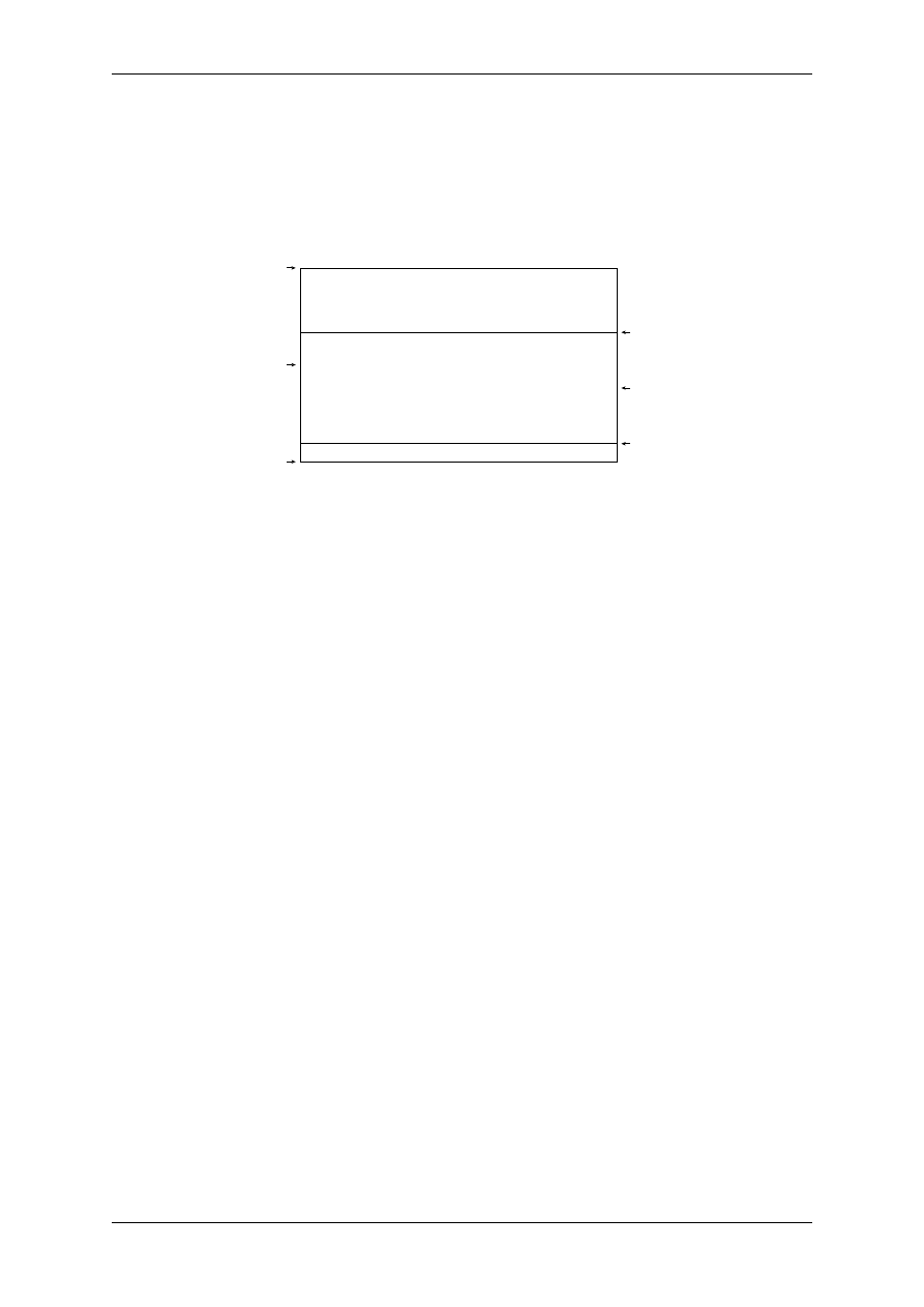
spam &
eggs
valign.top
valign.middle
valign.bottom
parbox.top
parbox.middle
parbox.bottom
Figure 7.1: valign example
class text.valign(valign)
Instances of this class set the vertical alignment of a text box to be top, center and bottom for valign being
0
, 0.5, and 1. Other values are allowed as well, although such an alignment seems quite unusual. See the
left side of figure
for an example.
Some handy instances available as class members:
valign.top
valign(0)
valign.middle
valign(0.5)
valign.bottom
valign(1)
valign.baseline
Identical to clearing the vertical alignment by clear to emphasise that a baseline alignment is not a box-
related alignment. Baseline alignment is the default, i.e. no valign is set by default.
class text.parbox(width, baseline=top)
Instances of this class create a box with a finite width, where the typesetter creates multiple lines in. Note,
that you can’t create multiple lines in TeX/LaTeX without specifying a box width. Since PyX doesn’t know
a box width, it uses TeXs LR-mode by default, which will always put everything into a single line. Since in
a vertical box there are several baselines, you can specify the baseline to be used by the optional baseline
argument. You can set it to the symbolic names top, parbox.middle, and parbox.bottom only,
which are members of
. See the right side of figure
for an example.
Since you need to specify a box width no predefined instances are available as class members.
class text.vshift(lowerratio, heightstr=”0”)
Instances of this class lower the output by lowerratio of the height of the string heigthstring. Note, that you
can apply several shifts to sum up the shift result. However, there is still a clear class member to remove
all vertical shifts.
Some handy instances available as class members:
vshift.bottomzero
vshift(0)
(this doesn’t shift at all)
26
Chapter 7. Module text: TeX/LaTeX interface

PyX Documentation, Release 0.11.1
vshift.middlezero
vshift(0.5)
vshift.topzero
vshift(1)
vshift.mathaxis
This is a special vertical shift to lower the output by the height of the mathematical axis. The mathematical
axis is used by TeX for the vertical alignment in mathematical expressions and is often usefull for vertical
alignment. The corresponding vertical shift is less than
and usually fits the height of the
minus sign. (It is the height of the minus sign in mathematical mode, since that’s that the mathematical axis
is all about.)
There is a TeX/LaTeX attribute to switch to TeXs math mode. The appropriate instances mathmode and
clearmathmode
(to clear the math mode attribute) are available at module level.
text.mathmode
Enables TeXs mathematical mode in display style.
The
class creates TeX/LaTeX attributes for changing the font size.
class text.size(sizeindex=None, sizename=None, sizelist=defaultsizelist)
LaTeX knows several commands to change the font size.
The command names are stored in
the sizelist, which defaults to ["normalsize", "large", "Large", "LARGE", "huge",
"Huge", None, "tiny", "scriptsize", "footnotesize", "small"]
.
You can either provide an index sizeindex to access an item in sizelist or set the command name by sizename.
Instances for the LaTeXs default size change commands are available as class members:
size.tiny
size(-4)
size.scriptsize
size(-3)
size.footnotesize
size(-2)
size.small
size(-1)
size.normalsize
size(0)
size.large
size(1)
size.Large
size(2)
size.LARGE
size(3)
size.huge
size(4)
size.Huge
size(5)
There is a TeX/LaTeX attribute to create empty text boxes with the size of the material passed in. The appropriate
instances phantom and clearphantom (to clear the phantom attribute) are available at module level.
text.phantom
Skip the text in the box, but keep its size.
7.3. TeX/LaTeX attributes
27

PyX Documentation, Release 0.11.1
7.4 Using the graphics-bundle with LaTeX
The packages in the LaTeX graphics bundle (color.sty, graphics.sty, graphicx.sty, ...) make ex-
tensive use of \\special commands. PyX defines a clean set of such commands to fit the needs of the LaTeX
graphics bundle. This is done via the pyx.def driver file, which tells the graphics bundle about the syntax
of the \\special commands as expected by PyX. You can install the driver file pyx.def into your LaTeX
search path and add the content of both files color.cfg and graphics.cfg to your personal configura-
tion files.
After you have installed the cfg files, please use the
module with unset pyxgraphics
keyword argument which will switch off a convenience hack for less experienced LaTeX users. You can then
import the LaTeX graphics bundle packages and related packages (e.g. rotating, ...) with the option pyx,
e.g. \\usepackage[pyx]{color,graphicx}. Note that the option pyx is only available with unset pyx-
graphics
keyword argument and a properly installed driver file. Otherwise, omit the specification of a driver when
loading the packages.
When you define colors in LaTeX via one of the color models gray, cmyk, rgb, RGB, hsb, then PyX will use
the corresponding values (one to four real numbers). In case you use any of the named colors in LaTeX, PyX
will use the corresponding predefined color (see module color and the color table at the end of the manual). The
additional LaTeX color model pyx allows to use a PyX color expression, such as color.cmyk(0,0,0,0)
directly in LaTeX. It is passed to PyX.
When importing Encapsulated PostScript files (eps files) PyX will rotate, scale and clip your file like you expect
it. Other graphic formats can not be imported via the graphics package at the moment.
For reference purpose, the following specials can be handled by PyX at the moment:
PyX:color_begin (model) (spec)
starts a color.
(model)
is one of gray, cmyk, rgb, hsb,
texnamed
, or pyxcolor. (spec) depends on the model: a name or some numbers
PyX:color_end
ends a color.
PyX:epsinclude file= llx= lly= urx= ury= width= height= clip=0/1
includes an En-
capsulated PostScript file (eps files). The values of llx to ury are in the files’ coordinate system and
specify the part of the graphics that should become the specified width and height in the outcome. The
graphics may be clipped. The last three parameters are optional.
PyX:scale_begin (x) (y)
begins scaling from the current point.
PyX:scale_end
ends scaling.
PyX:rotate_begin (angle)
begins rotation around the current point.
PyX:rotate_end
ends rotation.
7.5 TeX message parsers
Message parsers are used to scan the output of TeX/LaTeX. The output is analysed by a sequence of TeX message
parsers. Each message parser analyses the output and removes those parts of the output, it feels responsible for. If
there is nothing left in the end, the message got validated, otherwise an exception is raised reporting the problem.
A message parser might issue a warning when removing some output to give some feedback to the user.
class text.texmessage
This class acts as a container for TeX message parsers instances, which are all instances of classes derived
from
The following TeX message parser instances are available:
texmessage.start
Check for TeX/LaTeX startup message including scrollmode test.
texmessage.noaux
Ignore LaTeXs no-aux-file warning.
1
If you do not know what this is all about, you can just ignore this paragraph. But be sure that the pyxgraphics keyword argument is always
set!
28
Chapter 7. Module text: TeX/LaTeX interface

PyX Documentation, Release 0.11.1
texmessage.end
Check for proper TeX/LaTeX tear down message.
texmessage.load
Accepts arbitrary loading of files without checking for details, i.e. accept (file ...) where file is an
readable file.
texmessage.loaddef
Accepts arbitrary loading of fd files, i.e. accept (file.def) and (file.fd) where file.def or
file.fd
is an readable file, respectively.
texmessage.graphicsload
Accepts arbitrary loading of eps files, i.e. accept (file.eps) where file.eps is an readable file.
texmessage.ignore
Ignores everything (this is probably a bad idea, but sometimes you might just want to ignore everything).
texmessage.allwarning
Ignores everything but issues a warning.
texmessage.fontwarning
Issues a warning about font substitutions of the LaTeXs NFSS.
texmessage.boxwarning
Issues a warning on under- and overfull horizontal and vertical boxes.
class text.texmessagepattern(pattern, warning=None)
This is a derived class of
. It can be used to construct simple TeX message parsers, which
validate a TeX message matching a certain regular expression pattern pattern. When warning is set, a
warning message is issued. Several of the TeX message parsers described above are implemented using this
class.
7.6 The defaulttexrunner instance
text.defaulttexrunner
The defaulttexrunner is an instance of
. It is created when the
module is loaded
and it is used as the default texrunner instance by all
instances to implement its
method.
text.preamble(
...)
defaulttexrunner.preamble
text.text(
...)
defaulttexrunner.text
text.set(
...)
defaulttexrunner.set
text.reset(
...)
defaulttexrunner.reset
7.7 Some internals on temporary files etc.
It is not totally obvious how TeX processes are supervised by PyX and why it’s done that way. However there are
good reasons for it and the following description is intended for people wanting and/or needing to understand how
temporary files are used by PyX. All others don’t need to care.
Each time PyX needs to start a new TeX process, it creates a base file name for temporary files associated with
this process. This file name is used as \jobname by TeX. Since TeX does not handle directory names as part
of \jobname, the temporary files will be created in the current directory. The PyX developers decided to not
change the current directory at all, avoiding all kind of issues with accessing files in the local directory, like for
loading graph data, LaTeX style files etc.
7.6. The defaulttexrunner instance
29

PyX Documentation, Release 0.11.1
PyX creates a TeX file containing \relax only. It’s only use is to set TeXs \jobname. Immediately after
processing \relax TeX falls back to stdin to read more commands. PyX than uses stdin and stdout to
avoid various buffering issues which would occur when using files (or named pipes). By that PyX can fetch TeX
errors as soon as they occur while keeping the TeX process running (i.e. in a waiting state) for further input.
The size of the TeX output is also availble immediately without fetching the dvi file created by TeX, since PyX
uses some TeX macros to output the extents of the boxes created for the requested texts to stdout immediately.
There is a TeX hack --ipc which PyX knows to take advantage of to fetch informations from the dvi file
immediately as well, but it’s not available on all TeXinstallations. Thus this feature is disabled by default and
fetching informations from the dvi is tried to be limited to those cases, where no other option exists. By that TeX
usually doesn’t need to be started several times.
By default PyX will clean up all temporary files after TeX was stopped. However the usefiles list allows for a
renaming of the files from (and to, if existing) the temporary \jobname (+ suffix) handled by PyX. Additionally,
since PyX does not write a useful TeX input file in a file and thus a usefiles=["example.tex"] would not
contain the code actually passed to TeX, the texdebug feature of the texrunner can be used instead to get a the
full input passed to TeX.
In case you need to control the position where the temporary files are created (say, you’re working on a read-only
directory), the suggested solution is to switch the current directory before starting with text processing in PyX (i.e.
an os.chdir at the beginning of your script will do fine). You than just need to take care of specifying full paths
when accessing data from your original working directory, but that’s intended and necessary for that case.
30
Chapter 7. Module text: TeX/LaTeX interface

CHAPTER
EIGHT
GRAPHS
8.1 Introduction
PyX can be used for data and function plotting. At present x-y-graphs and x-y-z-graphs are supported only.
However, the component architecture of the graph system described in section
allows for
additional graph geometries while reusing most of the existing components.
Creating a graph splits into two basic steps. First you have to create a graph instance. The most simple form would
look like:
from
pyx
import
*
g
=
graph
.
graphxy(width
=
8
)
The graph instance g created in this example can then be used to actually plot something into the graph. Suppose
you have some data in a file graph.dat you want to plot. The content of the file could look like:
1
2
2
3
3
8
4
13
5
18
6
21
To plot these data into the graph g you must perform:
g
.
plot(graph
.
data
.
file(
"graph.dat"
, x
=
1
, y
=
2
))
The method plot() takes the data to be plotted and optionally a list of graph styles to be used to plot the data.
When no styles are provided, a default style defined by the data instance is used. For data read from a file by an
instance of
, the default are symbols. When instantiating
, you not
only specify the file name, but also a mapping from columns to axis names and other information the styles might
make use of (e.g. data for error bars to be used by the errorbar style).
While the graph is already created by that, we still need to perform a write of the result into a file. Since the graph
instance is a canvas, we can just call its writeEPSfile() method.
g
.
writeEPSfile(
"graph"
)
The result graph.eps is shown in figure
A minimalistic plot for the data from file graph.dat.
Instead of plotting data from a file, other data source are available as well. For example function data is created
and placed into plot() by the following line:
g
.
plot(graph
.
data
.
function(
"y(x)=x**2"
))
You can plot different data in a single graph by calling plot() several times before writeEPSfile() or
writePDFfile()
. Note that a calling plot() will fail once a graph was forced to “finish” itself. This
happens automatically, when the graph is written to a file. Thus it is not an option to call plot() after
writeEPSfile()
or writePDFfile(). The topic of the finalization of a graph is addressed in more detail
31
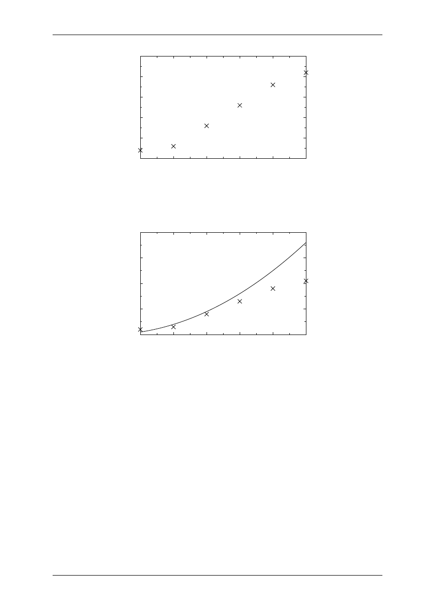
PyX Documentation, Release 0.11.1
1
2
3
4
5
6
0
5
10
15
20
25
Figure 8.1: A minimalistic plot for the data from file graph.dat.
in section
. As you can see in figure
Plotting data from a file together with a function.
, a function
is plotted as a line by default.
1
2
3
4
5
6
0
10
20
30
40
Figure 8.2: Plotting data from a file together with a function.
While the axes ranges got adjusted automatically in the previous example, they might be fixed by keyword options
in axes constructors. Plotting only a function will need such a setting at least in the variable coordinate. The
following code also shows how to set a logathmic axis in y-direction:
from
pyx
import
*
g
=
graph
.
graphxy(width
=
8
, x
=
graph
.
axis
.
linear(
min
=-
5
,
max
=
5
),
y
=
graph
.
axis
.
logarithmic())
g
.
plot(graph
.
data
.
function(
"y(x)=exp(x)"
))
g
.
writeEPSfile(
"graph3"
)
g
.
writePDFfile(
"graph3"
)
The result is shown in figure
Plotting a function for a given axis range and use a logarithmic y-axis.
8.2 Component architecture
Creating a graph involves a variety of tasks, which thus can be separated into components without significant
additional costs. This structure manifests itself also in the PyX source, where there are different modules for the
different tasks. They interact by some well-defined interfaces. They certainly have to be completed and stabilized
in their details, but the basic structure came up in the continuous development quite clearly. The basic parts of a
graph are:
32
Chapter 8. Graphs
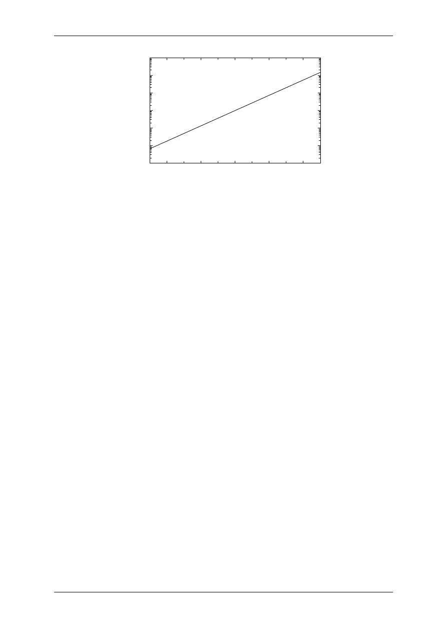
PyX Documentation, Release 0.11.1
0.001
0.01
0.1
1
10
100
1000
−4
−2
0
2
4
Figure 8.3: Plotting a function for a given axis range and use a logarithmic y-axis.
graph Defines the geometry of the graph by means of graph coordinates with range [0:1]. Keeps lists of plotted
data, axes etc.
data Produces or prepares data to be plotted in graphs.
style Performs the plotting of the data into the graph. It gets data, converts them via the axes into graph coordi-
nates and uses the graph to finally plot the data with respect to the graph geometry methods.
key Responsible for the graph keys.
axis Creates axes for the graph, which take care of the mapping from data values to graph coordinates. Because
axes are also responsible for creating ticks and labels, showing up in the graph themselves and other things,
this task is splitted into several independent subtasks. Axes are discussed separately in chapter axis.
8.3 Module graph.graph: Graph geometry
The classes
and
are part of the module
. However, there are shortcuts to
access the classes via graph.graphxy and graph.graphxyz, respectively.
class graph.graph.graphxy(xpos=0, ypos=0, width=None, height=None, ratio=goldenmean,
key=None
,
backgroundattrs=None
,
axesdist=0.8*unit.v_cm
,
xax-
isat=None
, yaxisat=None, **axes)
This class provides an x-y-graph. A graph instance is also a fully functional canvas.
The position of the graph on its own canvas is specified by xpos and ypos. The size of the graph is specified
by width, height, and ratio. These parameters define the size of the graph area not taking into account the
additional space needed for the axes. Note that you have to specify at least width or height. ratio will be
used as the ratio between width and height when only one of these is provided.
key
can be set to a
instance to create an automatic graph key. None omits the graph key.
backgroundattrs
is a list of attributes for drawing the background of the graph. Allowed are decorators,
strokestyles, and fillstyles. None disables background drawing.
axisdist
is the distance between axes drawn at the same side of a graph.
xaxisat
and yaxisat specify a value at the y and x axis, where the corresponding axis should be moved to.
It’s a shortcut for corresonding calls of
described below. Moving an axis by xaxisat or yaxisat
disables the automatic creation of a linked axis at the opposite side of the graph.
**axes
receives axes instances. Allowed keywords (axes names) are x, x2, x3, etc. and y, y2, y3, etc.
When not providing an x or y axis, linear axes instances will be used automatically. When not providing a
x2
or y2 axis, linked axes to the x and y axes are created automatically and vice versa. As an exception, a
linked axis is not created automatically when the axis is placed at a specific position by xaxisat or yaxisat.
You can disable the automatic creation of axes by setting the linked axes to None. The even numbered axes
8.3. Module graph.graph: Graph geometry
33

PyX Documentation, Release 0.11.1
are plotted at the top (x axes) and right (y axes) while the others are plotted at the bottom (x axes) and left
(y axes) in ascending order each.
Some instance attributes might be useful for outside read-access. Those are:
graphxy.axes
A dictionary mapping axes names to the anchoredaxis instances.
To actually plot something into the graph, the following instance method plot() is provided:
graphxy.plot(
data
, styles=None)
Adds data to the list of data to be plotted. Sets styles to be used for plotting the data. When styles is None,
the default styles for the data as provided by data is used.
data
should be an instance of any of the data described in section
When the same combination of styles (i.e. the same references) are used several times within the same graph
instance, the styles are kindly asked by the graph to iterate their appearance. Its up to the styles how this is
performed.
Instead of calling the plot method several times with different data but the same style, you can use a list (or
something iterateable) for data.
While a graph instance only collects data initially, at a certain point it must create the whole plot. Once this is done,
further calls of plot() will fail. Usually you do not need to take care about the finalization of the graph, because
it happens automatically once you write the plot into a file. However, sometimes position methods (described
below) are nice to be accessible. For that, at least the layout of the graph must have been finished. By calling the
do()
-methods yourself you can also alter the order in which the graph components are plotted. Multiple calls to
any of the do()-methods have no effect (only the first call counts). The orginal order in which the do()-methods
are called is:
graphxy.dolayout()
Fixes the layout of the graph. As part of this work, the ranges of the axes are fitted to the data when the
axes ranges are allowed to adjust themselves to the data ranges. The other do()-methods ensure, that this
method is always called first.
graphxy.dobackground()
Draws the background.
graphxy.doaxes()
Inserts the axes.
graphxy.doplotitem(
plotitem)
Plots the plotitem as returned by the graphs plot method.
graphxy.doplot()
Plots all (remaining) plotitems.
graphxy.dokeyitem()
Inserts a plotitem in the graph key as returned by the graphs plot method.
graphxy.dokey()
Inserts the graph key.
graphxy.finish()
Finishes the graph by calling all pending do()-methods. This is done automatically, when the output is
created.
The graph provides some methods to access its geometry:
graphxy.pos(
x
, y, xaxis=None, yaxis=None)
Returns the given point at x and y as a tuple (xpos, ypos) at the graph canvas. x and y are anchoredaxis
instances for the two axes xaxis and yaxis. When xaxis or yaxis are None, the axes with names x and y are
used. This method fails if called before
graphxy.vpos(
vx
, vy)
Returns the given point at vx and vy as a tuple (xpos, ypos) at the graph canvas. vx and vy are graph
coordinates with range [0:1].
34
Chapter 8. Graphs

PyX Documentation, Release 0.11.1
graphxy.vgeodesic(
vx1
, vy1, vx2, vy2)
Returns the geodesic between points vx1, vy1 and vx2, vy2 as a path. All parameters are in graph coordinates
with range [0:1]. For
this is a straight line.
graphxy.vgeodesic_el(
vx1
, vy1, vx2, vy2)
Like
but this method returns the path element to connect the two points.
Further geometry information is available by the axes instance variable, with is a dictionary mapping axis
names to anchoredaxis instances.
Shortcuts to the anchoredaxis positioner methods for the x- and y-
axis become available after dolayout() as
methods Xbasepath, Xvbasepath, Xgridpath,
Xvgridpath
, Xtickpoint, Xvtickpoint, Xtickdirection, and Xvtickdirection where the pre-
fix X stands for x and y.
graphxy.axistrafo(
axis
, t)
This method can be used to apply a transformation t to an anchoredaxis instance axis to modify the
axis position and the like. This method fails when called on a not yet finished axis, i.e. it should be used
after
graphxy.axisatv(
axis
, v)
This method calls
with a transformation to move the axis axis to a graph position v (in
graph coordinates).
The class
is very similar to the
class, except for its additional dimension. In the following
documentation only the differences to the
class are described.
class graph.graph.graphxyz(xpos=0,
ypos=0
,
size=None
,
xscale=1
,
yscale=1
,
zs-
cale=1/goldenmean
, projector=central(10, -30, 30), key=None,
**axes)
This class provides an x-y-z-graph.
The position of the graph on its own canvas is specified by xpos and ypos. The size of the graph is specified
by size and the length factors xscale, yscale, and zscale. The final size of the graph depends on the projector
projector
, which is called with x, y, and z values up to xscale, yscale, and zscale respectively and scaling
the result by size. For a parallel projector changing size is thus identical to changing xscale, yscale, and
zscale
by the same factor. For the central projector the projectors internal distance would also need to be
changed by this factor. Thus size changes the size of the whole graph without changing the projection.
projector
defines the conversion of 3d coordinates to 2d coordinates. It can be an instance of
or
described below.
**axes
receives axes instances as for
. The graphxyz allows for 4 axes per graph dimension x,
x2
, x3, x4, y, y2, y3, y4, z, z2, z3, and z4. The x-y-plane is the horizontal plane at the bottom and the
x
, x2, y, and y2 axes are placed at the boundary of this plane with x and y always being in front. x3, x4,
y3
, and y4 are handled similar, but for the top plane of the graph. The z axis is placed at the origin of the
x
and y dimension, whereas z2 is placed at the final point of the x dimension, z3 at the final point of the y
dimension and z4 at the final point of the x and y dimension together.
graphxyz.central
The central attribute of the graphxyz is the
class. See the class description below.
graphxyz.parallel
The parallel attribute of the graphxyz is the
class. See the class description below.
Regarding the 3d to 2d transformation the methods pos(), vpos(), vgeodesic(), and vgeodesic_el()
are available as for class
and just take an additional argument for the dimension. Note that a similar
transformation method (3d to 2d) is available as part of the projector as well already, but only the graph acknowl-
edges its size, the scaling and the internal tranformation of the graph coordinates to the scaled coordinates. As the
projector also implements a zindex() and a angle() method, those are also available at the graph level in the
graph coordinate variant (i.e. having an additional v in its name and using values from 0 to 1 per dimension).
graphxyz.vzindex(
vx
, vy, vz)
The depths of the point defined by vx, vy, and vz scaled to a range [-1:1] where 1 in closed to the viewer. All
arguments passed to the method are in graph coordinates with range [0:1].
8.3. Module graph.graph: Graph geometry
35

PyX Documentation, Release 0.11.1
graphxyz.vangle(
vx1
, vy1, vz1, vx2, vy2, vz2, vx3, vy3, vz3)
The cosine of the angle of the view ray thru point (vx1, vy1, vz1) and the plane defined by the
points (vx1, vy1, vz1), (vx2, vy2, vz2), and (vx3, vy3, vz3). All arguments passed to
the method are in graph coordinates with range [0:1].
There are two projector classes
and
class graph.graph.central(distance, phi, theta, anglefactor=math.pi/180)
Instances of this class implement a central projection for the given parameters.
distance
is the distance of the viewer from the origin. Note that the
class uses the range
-xscale
to xscale, -yscale to yscale, and -zscale to zscale for the coordinates x, y, and
z
. As those scales are of the order of one (by default), the distance should be of the order of 10 to give
nice results. Smaller distances increase the central projection character while for huge distances the central
projection becomes identical to the parallel projection.
phi
is the angle of the viewer in the x-y-plane and theta is the angle of the viewer to the x-y-plane.
The standard notation for spheric coordinates are used. The angles are multiplied by anglefactor which is
initialized to do a degree in radiant transformation such that you can specify phi and theta in degree
while the internal computation is always done in radiants.
class graph.graph.parallel(phi, theta, anglefactor=math.pi/180)
Instances of this class implement a parallel projection for the given parameters. There is no distance for
that transformation (compared to the central projection). All other parameters are identical to the
class.
8.4 Module graph.data: Graph data
The following classes provide data for the plot() method of a graph.
The classes are implemented in
class graph.data.file(filename,
commentpattern=defaultcommentpattern
,
columnpat-
tern=defaultcolumnpattern
, stringpattern=defaultstringpattern, skiphead=0,
skiptail=0
, every=1, title=notitle, context={}, copy=1, replacedollar=1,
columncallback=”__column__”
, **columns)
This class reads data from a file and makes them available to the graph system. filename is the name of the
file to be read. The data should be organized in columns.
The arguments commentpattern, columnpattern, and stringpattern are responsible for identifying the data
in each line of the file. Lines matching commentpattern are ignored except for the column name search of
the last non- empty comment line before the data. By default a line starting with one of the characters ’#’,
’%’
, or ’!’ as well as an empty line is treated as a comment.
A non-comment line is analysed by repeatedly matching stringpattern and, whenever the stringpattern does
not match, by columnpattern. When the stringpattern matches, the result is taken as the value for the next
column without further transformations. When columnpattern matches, it is tried to convert the result to a
float. When this fails the result is taken as a string as well. By default, you can write strings with spaces
surrounded by ’"’ immediately surrounded by spaces or begin/end of line in the data file. Otherwise ’"’
is not taken to be special.
skiphead
and skiptail are numbers of data lines to be ignored at the beginning and end of the file while every
selects only every every line from the data.
title
is the title of the data to be used in the graph key. A default title is constructed out of filename and
**columns
. You may set title to None to disable the title.
Finally, columns define columns out of the existing columns from the file by a column number or a mathe-
matical expression (see below). When copy is set the names of the columns in the file (file column names)
and the freshly created columns having the names of the dictionary key (data column names) are passed as
data to the graph styles. The data columns may hide file columns when names are equal. For unset copy the
file columns are not available to the graph styles.
36
Chapter 8. Graphs

PyX Documentation, Release 0.11.1
File column names occur when the data file contains a comment line immediately in front of the data (except
for empty or empty comment lines). This line will be parsed skipping the matched comment identifier as if
the line would be regular data, but it will not be converted to floats even if it would be possible to convert
the items. The result is taken as file column names, i.e. a string representation for the columns in the file.
The values of **columns can refer to column numbers in the file starting at 1. The column 0 is also available
and contains the line number starting from 1 not counting comment lines, but lines skipped by skiphead,
skiptail
, and every. Furthermore values of **columns can be strings: file column names or complex math-
ematical expressions. To refer to columns within mathematical expressions you can also use file column
names when they are valid variable identifiers. Equal named items in context will then be hidden. Alterna-
tively columns can be access by the syntax $<number> when replacedollar is set. They will be translated
into function calls to columncallback, which is a function to access column data by index or name.
context
allows for accessing external variables and functions when evaluating mathematical expressions for
columns. Additionally to the identifiers in context, the file column names, the columncallback function and
the functions shown in the table “builtins in math expressions” at the end of the section are available.
Example:
graph
.
data
.
file(
"test.dat"
, a
=
1
, b
=
"B"
, c
=
"2*B+$3"
)
with test.dat looking like:
# A
B C
1.234 1 2
5.678 3 4
The columns with name "a", "b", "c" will become "[1.234, 5.678]", "[1.0, 3.0]", and
"[4.0, 10.0]"
, respectively. The columns "A", "B", "C" will be available as well, since copy is
enabled by default.
When creating several data instances accessing the same file, the file is read only once. There is an inherent
caching of the file contents.
For the sake of completeness we list the default patterns:
file.defaultcommentpattern
re.compile(r"(#+|!+|%+)\s*")
file.defaultcolumnpattern
re.compile(r"\"(.*?)\"(\s+|$)")
file.defaultstringpattern
re.compile(r"(.*?)(\s+|$)")
class graph.data.function(expression, title=notitle, min=None, max=None, points=100, con-
text={})
This class creates graph data from a function. expression is the mathematical expression of the function. It
must also contain the result variable name including the variable the function depends on by assignment. A
typical example looks like "y(x)=sin(x)".
title
is the title of the data to be used in the graph key. By default expression is used. You may set title to
None
to disable the title.
min
and max give the range of the variable. If not set, the range spans the whole axis range. The axis range
might be set explicitly or implicitly by ranges of other data. points is the number of points for which the
function is calculated. The points are choosen linearly in terms of graph coordinates.
context
allows for accessing external variables and functions. Additionally to the identifiers in context, the
variable name and the functions shown in the table “builtins in math expressions” at the end of the section
are available.
class graph.data.paramfunction(varname, min, max, expression, title=notitle, points=100, con-
text={})
This class creates graph data from a parametric function. varname is the parameter of the function. min and
8.4. Module graph.data: Graph data
37

PyX Documentation, Release 0.11.1
max
give the range for that variable. points is the number of points for which the function is calculated. The
points are choosen lineary in terms of the parameter.
expression
is the mathematical expression for the parametric function. It contains an assignment of a tuple
of functions to a tuple of variables. A typical example looks like "x, y = cos(k), sin(k)".
title
is the title of the data to be used in the graph key. By default expression is used. You may set title to
None
to disable the title.
context
allows for accessing external variables and functions. Additionally to the identifiers in context,
varname
and the functions shown in the table “builtins in math expressions” at the end of the section are
available.
class graph.data.values(title=”user provided values”, **columns)
This class creates graph data from externally provided data. Each column is a list of values to be used for
that column.
title
is the title of the data to be used in the graph key.
class graph.data.points(data, title=”user provided points”, addlinenumbers=1, **columns)
This class creates graph data from externally provided data. data is a list of lines, where each line is a list
of data values for the columns.
title
is the title of the data to be used in the graph key.
The keywords of **columns become the data column names. The values are the column numbers starting
from one, when addlinenumbers is turned on (the zeroth column is added to contain a line number in that
case), while the column numbers starts from zero, when addlinenumbers is switched off.
class graph.data.data(data,
title=notitle
,
context=
,
copy=1
,
replacedollar=1
,
columncall-
back=”__column__”
, **columns)
This class provides graph data out of other graph data. data is the source of the data. All other parameters
work like the equally called parameters in
. Indeed, the latter is built on top of this
class by reading the file and caching its contents in a graph.data.list instance.
class graph.data.conffile(filename, title=notitle, context=, copy=1, replacedollar=1, columncall-
back=”__column__”
, **columns)
This class reads data from a config file with the file name filename. The format of a config file is described
within the documentation of the ConfigParser module of the Python Standard Library.
Each section of the config file becomes a data line. The options in a section are the columns. The name
of the options will be used as file column names. All other parameters work as in graph.data.file and
graph.data.data
since they all use the same code.
class graph.data.cbdfile(filename,
minrank=None
,
maxrank=None
,
title=notitle
,
context=
,
copy=1
, replacedollar=1, columncallback=”__column__”, **columns)
This
is
an
experimental
class
to
read
map
data
from
cbd-files.
See
http://sepwww.stanford.edu/ftp/World_Map/
for some world-map data.
The builtins in math expressions are listed in the following table:
38
Chapter 8. Graphs

PyX Documentation, Release 0.11.1
name
value
neg
lambda x:
-x
abs
lambda x:
x < 0 and -x or x
sgn
lambda x:
x < 0 and -1 or 1
sqrt
math.sqrt
exp
math.exp
log
math.log
sin
math.sin
cos
math.cos
tan
math.tan
asin
math.asin
acos
math.acos
atan
math.atan
sind
lambda x:
math.sin(math.pi/180*x)
cosd
lambda x:
math.cos(math.pi/180*x)
tand
lambda x:
math.tan(math.pi/180*x)
asind
lambda x:
180/math.pi*math.asin(x)
acosd
lambda x:
180/math.pi*math.acos(x)
atand
lambda x:
180/math.pi*math.atan(x)
norm
lambda x, y:
math.hypot(x, y)
splitatvalue
see the splitatvalue description below
pi
math.pi
e
math.e
math
refers to Pythons math module. The splitatvalue function is defined as:
graph.data.splitatvalue(
value
, *splitpoints)
This method returns a tuple (section, value). The section is calculated by comparing value with the
values of splitpoints. If splitpoints contains only a single item, section is 0 when value is lower or equal
this item and 1 else. For multiple splitpoints, section is 0 when its lower or equal the first item, None
when its bigger than the first item but lower or equal the second item, 1 when its even bigger the second
item, but lower or equal the third item. It continues to alter between None and 2, 3, etc.
8.5 Module graph.style: Graph styles
Please note that we are talking about graph styles here. Those are responsible for plotting symbols, lines, bars
and whatever else into a graph. Do not mix it up with path styles like the line width, the line style (solid, dashed,
dotted etc.) and others.
The following classes provide styles to be used at the plot() method of a graph. The plot method accepts a list
of styles. By that you can combine several styles at the very same time.
Some of the styles below are hidden styles. Those do not create any output, but they perform internal data handling
and thus help on modularization of the styles. Usually, a visible style will depend on data provided by one or more
hidden styles but most of the time it is not necessary to specify the hidden styles manually. The hidden styles
register themself to be the default for providing certain internal data.
class graph.style.pos(epsilon=1e-10)
This class is a hidden style providing a position in the graph. It needs a data column for each graph dimen-
sion. For that the column names need to be equal to an axis name. Data points are considered to be out of
graph when their position in graph coordinates exceeds the range [0:1] by more than epsilon.
class graph.style.range(usenames=, epsilon=1e-10)
This class is a hidden style providing an errorbar range. It needs data column names constructed out of a
axis name X for each dimension errorbar data should be provided as follows:
8.5. Module graph.style: Graph styles
39

PyX Documentation, Release 0.11.1
data name
description
Xmin
minimal value
Xmax
maximal value
dX
minimal and maximal delta
dXmin
minimal delta
dXmax
maximal delta
When delta data are provided the style will also read column data for the axis name X itself. usenames
allows to insert a translation dictionary from axis names to the identifiers X.
epsilon
is a comparison precision when checking for invalid errorbar ranges.
class graph.style.symbol(symbol=changecross, size=0.2*unit.v_cm, symbolattrs=
[ ]
)
This class is a style for plotting symbols in a graph. symbol refers to a (changeable) symbol function with the
prototype symbol(c, x_pt, y_pt, size_pt, attrs) and draws the symbol into the canvas c
at the position (x_pt, y_pt) with size size_pt and attributes attrs. Some predefined symbols are
available in member variables listed below. The symbol is drawn at size size using symbolattrs. symbolattrs
is merged with defaultsymbolattrs which is a list containing the decorator deco.stroked. An
instance of
is the default style for all graph data classes described in section
except
for function and paramfunction.
The class
provides some symbol functions as member variables, namely:
symbol.cross
A cross. Should be used for stroking only.
symbol.plus
A plus. Should be used for stroking only.
symbol.square
A square. Might be stroked or filled or both.
symbol.triangle
A triangle. Might be stroked or filled or both.
symbol.circle
A circle. Might be stroked or filled or both.
symbol.diamond
A diamond. Might be stroked or filled or both.
provides some changeable symbol functions as member variables, namely:
symbol.changecross
attr.changelist([cross, plus, square, triangle, circle, diamond])
symbol.changeplus
attr.changelist([plus, square, triangle, circle, diamond, cross])
symbol.changesquare
attr.changelist([square, triangle, circle, diamond, cross, plus])
symbol.changetriangle
attr.changelist([triangle, circle, diamond, cross, plus, square])
symbol.changecircle
attr.changelist([circle, diamond, cross, plus, square, triangle])
symbol.changediamond
attr.changelist([diamond, cross, plus, square, triangle, circle])
symbol.changesquaretwice
attr.changelist([square, square, triangle, triangle, circle, circle, diamond, diamond])
symbol.changetriangletwice
attr.changelist([triangle, triangle, circle, circle, diamond, diamond, square, square])
40
Chapter 8. Graphs

PyX Documentation, Release 0.11.1
symbol.changecircletwice
attr.changelist([circle, circle, diamond, diamond, square, square, triangle, triangle])
symbol.changediamondtwice
attr.changelist([diamond, diamond, square, square, triangle, triangle, circle, circle])
The class
provides two changeable decorators for alternated filling and stroking. Those are especially
useful in combination with the change()-twice()-symbol methods above. They are:
symbol.changestrokedfilled
attr.changelist([deco.stroked, deco.filled])
symbol.changefilledstroked
attr.changelist([deco.filled, deco.stroked])
class graph.style.line(lineattrs=
[ ]
)
This class is a style to stroke lines in a graph. lineattrs is merged with defaultlineattrs which is a list
containing the member variable changelinestyle as described below. An instance of
is the de-
fault style of the graph data classes function and paramfunction described in section
The class
provides a changeable line style. Its definition is:
line.changelinestyle
attr.changelist([style.linestyle.solid,
style.linestyle.dashed,
style.linestyle.dotted,
style.linestyle.dashdotted])
class graph.style.impulses(lineattrs=
[ ]
, fromvalue=0, frompathattrs=
[ ]
, valueaxisindex=1)
This class is a style to plot impulses. lineattrs is merged with defaultlineattrs which is a list con-
taining the member variable changelinestyle of the
class. fromvalue is the baseline value of the
impulses. When set to None, the impulses will start at the baseline. When fromvalue is set, frompathattrs
are the stroke attributes used to show the impulses baseline path.
class graph.style.errorbar(size=0.1*unit.v_cm, errorbarattrs=
[ ]
, epsilon=1e-10)
This class is a style to stroke errorbars in a graph. size is the size of the caps of the errorbars and errorbarattrs
are the stroke attributes. Errorbars and error caps are considered to be out of the graph when their position
in graph coordinates exceeds the range [0:1] by more that epsilon. Out of graph caps are omitted and the
errorbars are cut to the valid graph range.
class graph.style.text(textname=”text”, dxname=None, dyname=None, dxunit=0.3*unit.v_cm,
dyunit=0.3*unit.v_cm
, textdx=0*unit.v_cm, textdy=0.3*unit.v_cm, textat-
trs=
[ ]
)
This class is a style to stroke text in a graph. The text to be written has to be provided in the data column
named textname. textdx and textdy are the position of the text with respect to the position in the graph.
Alternatively you can specify a dxname and a dyname and provide appropriate data in those columns
to be taken in units of dxunit and dyunit to specify the position of the text for each point separately. tex-
tattrs
are text attributes for the output of the text. Those attributes are merged with the default attributes
textmodule.halign.center
and textmodule.vshift.mathaxis.
class graph.style.arrow(linelength=0.25*unit.v_cm, arrowsize=0.15*unit.v_cm, lineattrs=
[ ]
, ar-
rowattrs=
[ ]
, arrowpos=0.5, epsilon=1e-10, decorator=deco.earrow)
This class is a style to plot short lines with arrows into a two-dimensional graph to a given graph position.
The arrow parameters are defined by two additional data columns named size and angle define the size
and angle for each arrow. size is taken as a factor to arrowsize and linelength, the size of the arrow and the
length of the line the arrow is plotted at. angle is the angle the arrow points to with respect to a horizontal
line. The angle is taken in degrees and used in mathematically positive sense. lineattrs and arrowattrs are
styles for the arrow line and arrow head, respectively. arrowpos defines the position of the arrow line with
respect to the position at the graph. The default 0.5 means centered at the graph position, whereas 0 and
1
creates the arrows to start or end at the graph position, respectively. epsilon is used as a cutoff for short
arrows in order to prevent numerical instabilities. decorator defines the decorator to be added to the line.
class graph.style.rect(gradient=color.gradient.Grey)
This class is a style to plot colored rectangles into a two-dimensional graph. The size of the rectangles is
taken from the data provided by the
style. The additional data column named color specifies the
color of the rectangle defined by gradient. The valid color range is [0:1].
8.5. Module graph.style: Graph styles
41

PyX Documentation, Release 0.11.1
class graph.style.histogram(lineattrs=
[ ]
, steps=0, fromvalue=0, frompathattrs=
[ ]
, fillable=0,
rectkey=0
, autohistogramaxisindex=0, autohistogrampointpos=0.5,
epsilon=1e-10)
This class is a style to plot histograms.
lineattrs
is merged with defaultlineattrs which is
[deco.stroked]
. When steps is set, the histrogram is plotted as steps instead of the default being a
boxed histogram. fromvalue is the baseline value of the histogram. When set to None, the histogram
will start at the baseline. When fromvalue is set, frompathattrs are the stroke attributes used to show the
histogram baseline path.
The fillable flag changes the stoke line of the histogram to make it fillable properly. This is important on
non-steped histograms or on histograms, which hit the graph boundary. rectkey can be set to generate a
rectanglar area instead of a line in the graph key.
In the most general case, a histogram is defined by a range specification (like for an errorbar) in one graph
dimension (say, along the x-axis) and a value for the other graph dimension. This allows for the widths of the
histogram boxes being variable. Often, however, all histogram bin ranges are equally sized, and instead of
passing the range, the position of the bin along the x-axis fully specifies the histogram - assuming that there
are at least two bins. This common case is supported via two parameters: autohistogramaxisindex, which
defines the index of the independent histogram axis (in the case just described this would be 0 designating
the x axis). autohistogrampointpos, defines the relative position of the center of the histogram bin: 0.5
means that the bin is centered at the values passed to the style, 0 (1) means that the bin is aligned at the
right-(left-)hand side.
XXX describe, how to specify general histograms with varying bin widths
Positions of the histograms are considered to be out of graph when they exceed the graph coordinate range
[0:1] by more than epsilon.
class graph.style.barpos(fromvalue=None, frompathattrs=
[ ]
, epsilon=1e-10)
This class is a hidden style providing position information in a bar graph. Those graphs need to contain a
specialized axis, namely a bar axis. The data column for this bar axis is named Xname where X is an axis
name. In the other graph dimension the data column name must be equal to an axis name. To plot several
bars in a single graph side by side, you need to have a nested bar axis and provide a tuple as data for nested
bar axis.
The bars start at fromvalue when provided. The fromvalue is marked by a gridline stroked using frompathat-
trs
. Thus this hidden style might actually create some output. The value of a bar axis is considered to be out
of graph when its position in graph coordinates exceeds the range [0:1] by more than epsilon.
class graph.style.stackedbarpos(stackname, addontop=0, epsilon=1e-10)
This class is a hidden style providing position information in a bar graph by stacking a new bar on top of
another bar. The value of the new bar is taken from the data column named stackname. When addontop is
set, the values is taken relative to the previous top of the bar.
class graph.style.bar(barattrs=
[ ]
, epsilon=1e-10, gradient=color.gradient.RedBlack)
This class draws bars in a bar graph.
The bars are filled using barattrs.
barattrs
is
merged with defaultbarattrs which is a list containing [color.gradient.Rainbow,
deco.stroked([color.grey.black])]
.
The bar style has limited support for 3d graphs: Occlusion does not work properly on stacked bars or
multiple dataset. epsilon is used in 3d to prevent numerical instabilities on bars without hight. When
gradient
is not None it is used to calculate a lighting coloring taking into account the angle between the
view ray and the bar and the distance between viewer and bar. The precise conversion is defined in the
lighting()
method.
class graph.style.changebar(barattrs=
[ ]
)
This style works like the
style, but instead of the barattrs to be changed on subsequent data instances
the barattrs are changed for each value within a single data instance. In the result the style can’t be applied
to several data instances and does not support 3d. The style raises an error instead.
class graph.style.gridpos(index1=0,
index2=1
,
gridlines1=1
,
gridlines2=1
,
gridattrs=
[ ]
,
epsilon=1e-10)
This class is a hidden style providing rectangular grid information out of graph positions for graph dimen-
sions index1 and index2. Data points are considered to be out of graph when their position in graph coor-
42
Chapter 8. Graphs

PyX Documentation, Release 0.11.1
dinates exceeds the range [0:1] by more than epsilon. Data points are merged to a single graph coordinate
value when their difference in graph coordinates is below epsilon.
class graph.style.grid(gridlines1=1, gridlines2=1, gridattrs=
[ ]
)
Strokes a rectangular grid in the first grid direction, when gridlines1 is set and in the second grid direction,
when gridlines2 is set. gridattrs is merged with defaultgridattrs which is a list containing the
member variable changelinestyle of the
class.
class graph.style.surface(colorname=”color”, gradient=color.gradient.Grey, mincolor=None,
maxcolor=None
, gridlines1=0.05, gridlines2=0.05, gridcolor=None,
backcolor=color.gray.black)
Draws a surface of a rectangular grid. Each rectangle is divided into 4 triangles.
The grid can be colored using values provided by the data column named colorname. The values are rescaled
to the range [0:1] using mincolor and maxcolor (which are taken from the minimal and maximal values, but
larger bounds could be set).
If no colorname column exists, the surface style falls back to a lighting coloring taking into account the
angle between the view ray and the triangle and the distance between viewer and triangle. The precise
conversion is defined in the lighting() method.
If a gridcolor is set, the rectangular grid is marked by small stripes of the relative (compared to each
rectangle) size of gridlines1 and gridlines2 for the first and second grid direction, respectively.
backcolor
is used to fill triangles shown from the back. If backcolor is set to None, back sides are not
drawn differently from the front sides.
The surface is encoded using a single mesh. While this is quite space efficient, it has the following implica-
tions:
• All colors must use the same color space.
• HSB colors are not allowed, whereas Gray, RGB, and CMYK are allowed. You can convert HSB col-
ors into a different color space before passing them to the surface.
• The grid itself is also constructed out of triangles. The grid is transformed along with the triangles
thus looking quite different from a stroked grid (as done by the grid style).
• Occlusion is handled by proper painting order.
• Color changes are continuous (in the selected color space) for each triangle.
8.6 Module graph.key: Graph keys
The following class provides a key, whose instances can be passed to the constructor keyword argument key of a
graph. The class is implemented in
class graph.key.key(dist=0.2*unit.v_cm, pos=”tr”, hpos=None, vpos=None, hinside=1, vinside=1,
hdist=0.6*unit.v_cm
,
vdist=0.4*unit.v_cm
,
symbolwidth=0.5*unit.v_cm
,
symbolheight=0.25*unit.v_cm
,
symbolspace=0.2*unit.v_cm
,
textattrs=
[ ]
,
columns=1
, columndist=0.5*unit.v_cm, border=0.3*unit.v_cm, keyattrs=None)
This class writes the title of the data in a plot together with a small illustration of the style. The style is
responsible for its illustration.
dist
is a visual length and a distance between the key entries. pos is the position of the key with respect to
the graph. Allowed values are combinations of "t" (top), "m" (middle) and "b" (bottom) with "l" (left),
"c"
(center) and "r" (right). Alternatively, you may use hpos and vpos to specify the relative position
using the range [0:1]. hdist and vdist are the distances from the specified corner of the graph. hinside and
vinside
are numbers to be set to 0 or 1 to define whether the key should be placed horizontally and vertically
inside of the graph or not.
symbolwidth
and symbolheight are passed to the style to control the size of the style illustration. symbolspace
is the space between the illustration and the text. textattrs are attributes for the text creation. They are merged
with [text.vshift.mathaxis].
8.6. Module graph.key: Graph keys
43

PyX Documentation, Release 0.11.1
columns
is a number of columns of the graph key and columndist is the distance between those columns.
When keyattrs is set to contain some draw attributes, the graph key is enlarged by border and the key area
is drawn using keyattrs.
44
Chapter 8. Graphs

CHAPTER
NINE
AXES
9.1 Component architecture
Axes are a fundamental component of graphs although there might be applications outside of the graph system.
Internally axes are constructed out of components, which handle different tasks axes need to fulfill:
axis Implements the conversion of a data value to a graph coordinate of range [0:1]. It does also handle the proper
usage of the components in complicated tasks (i.e. combine the partitioner, texter, painter and rater to find
the best partitioning).
An anchoredaxis is a container to combine an axis with an positioner and provide a storage area for all kind
of axis data. That way axis instances are reusable (they do not store any data locally). The anchoredaxis
and the positioner are created by a graph corresponding to its geometry.
tick Ticks are plotted along the axis. They might be labeled with text as well.
partitioner, we use “parter” as a short form Creates one or several choices of tick lists suitable to a certain axis
range.
texter Creates labels for ticks when they are not set manually.
painter Responsible for painting the axis.
rater Calculate ratings, which can be used to select the best suitable partitioning.
positioner Defines the position of an axis.
The names above map directly to modules which are provided in the directory graph/axis except for the
anchoredaxis, which is part of the axis module as well. Sometimes it might be convenient to import the axis
directory directly rather than to access iit through the graph. This would look like:
from
pyx
import
*
graph
.
axis
.
painter()
# and the like
from
pyx.graph
import
axis
axis
.
painter()
# this is shorter ...
In most cases different implementations are available through different classes, which can be combined in various
ways. There are various axis examples distributed with PyX, where you can see some of the features of the axis
with a few lines of code each. Hence we can here directly come to the reference of the available components.
9.2 Module graph.axis.axis: Axes
The following classes are part of the module
. However, there is a shortcut to access those
classes via graph.axis directly.
Instances of the following classes can be passed to the **axes keyword arguments of a graph. Those instances
should only be used once.
45

PyX Documentation, Release 0.11.1
class graph.axis.axis.linear(min=None, max=None, reverse=0, divisor=None, title=None,
parter=parter.autolinear()
,
manualticks=
[ ]
,
density=1
,
maxworse=2
,
rater=rater.linear()
,
texter=texter.mixed()
,
painter=painter.regular()
,
linkpainter=painter.linked()
,
fall-
backrange=None)
This class provides a linear axis. min and max define the axis range. When not set, they are adjusted
automatically by the data to be plotted in the graph. Note, that some data might want to access the range of
an axis (e.g. the function class when no range was provided there) or you need to specify a range when
using the axis without plugging it into a graph (e.g. when drawing an axis along a path). In cases where the
data provides a range of zero (e.g. a when plotting a constant function), then a fallbackrange can be set to
guarantee a minimal range of the axis.
reverse
can be set to indicate a reversed axis starting with bigger values first. Alternatively you can fix the
axis range by min and max accordingly. When divisor is set, it is taken to divide all data range and position
informations while creating ticks. You can create ticks not taking into account a factor by that. title is the
title of the axis.
parter
is a partitioner instance, which creates suitable ticks for the axis range. Those ticks are merged with
ticks manually given by manualticks before proceeding with rating, painting etc. Manually placed ticks
win against those created by the partitioner. For automatic partitioners, which are able to calculate several
possible tick lists for a given axis range, the density is a (linear) factor to favour more or less ticks. It should
not be stressed to much (its likely, that the result would be unappropriate or not at all valid in terms of rating
label distances). But within a range of say 0.5 to 2 (even bigger for large graphs) it can help to get less or
more ticks than the default would lead to. maxworse is the number of trials with more and less ticks when
a better rating was already found. rater is a rater instance, which rates the ticks and the label distances for
being best suitable. It also takes into account density. The rater is only needed, when the partitioner creates
several tick lists.
texter
is a texter instance. It creates labels for those ticks, which claim to have a label, but do not have a label
string set already. Ticks created by partitioners typically receive their label strings by texters. The painter
is finally used to construct the output. Note, that usually several output constructions are needed, since the
rater is also used to rate the distances between the labels for an optimum. The linkedpainter is used as the
axis painter, when automatic link axes are created by the createlinked() method.
class graph.axis.axis.lin(...)
This class is an abbreviation of
described above.
class graph.axis.axis.logarithmic(min=None, max=None, reverse=0, divisor=None, ti-
tle=None
, parter=parter.autologarithmic(), manualticks=
[
]
,
density=1
,
maxworse=2
,
rater=rater.logarithmic()
,
texter=texter.mixed()
,
painter=painter.regular()
,
linkpainter=painter.linked()
, fallbackrange=None)
This class provides a logarithmic axis. All parameters work like
. Only two parameters have a
different default: parter and rater. Furthermore and most importantly, the mapping between data and graph
coordinates is logarithmic.
class graph.axis.axis.log(...)
This class is an abbreviation of
described above.
class graph.axis.axis.bar(subaxes=None,
defaultsubaxis=linear(painter=None
,
linkpainter=None
,
parter=None
,
texter=None)
,
dist=0.5
,
firstdist=None
,
lastdist=None
,
title=None
,
reverse=0
,
painter=painter.bar()
, linkpainter=painter.linkedbar())
This class provides an axis suitable for a bar style. It handles a discrete set of values and maps them to
distinct ranges in graph coordinates. For that, the axis gets a tuple of two values.
The first item is taken to be one of the discrete values valid on this axis. The discrete values can be any
hashable type and the order of the subaxes is defined by the order the data is received or the inverse of that
when reverse is set.
The second item is passed to the corresponding subaxis. The result of the conversion done by the subaxis
is mapped to the graph coordinate range reserved for this subaxis. This range is defined by a size attribute
of the subaxis, which can be added to any axis. (see the sized linear axes described below for some axes
46
Chapter 9. Axes

PyX Documentation, Release 0.11.1
already having a size argument). When no size information is available for a subaxis, a size value of 1 is
used. The baraxis itself calculates its size by suming up the sizes of its subaxes plus firstdist, lastdist and
dist
times the number of subaxes minus 1.
subaxes
should be a list or a dictionary mapping a discrete value of the bar axis to the corresponding subaxis.
When no subaxes are set or data is received for an unknown discrete axis value, instances of defaultsubaxis
are used as the subaxis for this discrete value.
dist
is used as the spacing between the ranges for each distinct value. It is measured in the same units as the
subaxis results, thus the default value of 0.5 means half the width between the distinct values as the width
for each distinct value. firstdist and lastdist are used before the first and after the last value. When set to
None
, half of dist is used.
title
is the title of the split axes and painter is a specialized painter for an bar axis and linkpainter is used as
the painter, when automatic link axes are created by the createlinked() method.
class graph.axis.axis.nestedbar(subaxes=None, defaultsubaxis=bar(dist=0, painter=None,
linkpainter=None)
,
dist=0.5
,
firstdist=None
,
last-
dist=None
, title=None, reverse=0, painter=painter.bar(),
linkpainter=painter.linkedbar())
This class is identical to the bar axis except for the different default value for defaultsubaxis.
class graph.axis.axis.split(subaxes=None,
defaultsubaxis=linear()
,
dist=0.5
,
firstdist=0
,
lastdist=0
,
title=None
,
reverse=0
,
painter=painter.split()
,
linkpainter=painter.linkedsplit())
This class is identical to the bar axis except for the different default value for defaultsubaxis, firstdist,
lastdist, painter, and linkedpainter.
Sometimes you want to alter the default size of 1 of the subaxes. For that you have to add a size attribute to the
axis data. The two classes sizedlinear and autosizedlinear do that for linear axes. Their short names
are sizedlin and autosizedlin. sizedlinear extends the usual linear axis by an first argument size.
autosizedlinear
creates the size out of its data range automatically but sets an autolinear parter with
extendtick
being None in order to disable automatic range modifications while painting the axis.
The axis module also contains classes implementing so called anchored axes, which combine an axis with an
positioner and a storage place for axis related data. Since these features are not interesting for the average PyX
user, we’ll not go into all the details of their parameters and except for some handy axis position methods:
class graph.axis.axis.anchoredaxis
anchoredaxis.basepath(
x1=None
, x2=None)
Returns a path instance for the base path. x1 and x2 define the axis range, the base path should cover.
For None the beginning and end of the path is taken, which might cover a longer range, when the axis is
embedded as a subaxis. For that case, a None value extends the range to the point of the middle between
two subaxes or the beginning or end of the whole axis, when the subaxis is the first or last of the subaxes.
anchoredaxis.vbasepath(
v1=None
, v2=None)
Like
but in graph coordinates.
anchoredaxis.gridpath(
x)
Returns a path instance for the grid path at position x. Might return None when no grid path is available.
anchoredaxis.vgridpath(
v)
Like
but in graph coordinates.
anchoredaxis.tickpoint(
x)
Returns the position of x as a tuple (x, y).
anchoredaxis.vtickpoint(
v)
Like
but in graph coordinates.
anchoredaxis.tickdirection(
x)
Returns the direction of a tick at x as a tuple (dx, dy). The tick direction points inside of the graph.
anchoredaxis.vtickdirection(
v)
Like
but in graph coordinates.
9.2. Module graph.axis.axis: Axes
47

PyX Documentation, Release 0.11.1
anchoredaxis.vtickdirection(
v)
Like
but in graph coordinates.
However, there are two anchored axes implementations
and
which are
available to the user to create special forms of anchored axes.
class graph.axis.axis.linkedaxis(linkedaxis=None,
errorname=”manual-linked”
,
painter=_marker)
This class implements an anchored axis to be passed to a graph constructor to manually link the axis to
another anchored axis instance linkedaxis. Note that you can skip setting the value of linkedaxis in the
constructor, but set it later on by the
method described below. errorname is printed
within error messages when the data is used and some problem occurs. painter is used for painting the
linked axis instead of the linkedpainter provided by the linkedaxis.
linkedaxis.setlinkedaxis(
linkedaxis)
This method can be used to set the linkedaxis after constructing the axis. By that you can create several
graph instances with cycled linked axes.
class graph.axis.axis.anchoredpathaxis(path, axis, direction=1)
This class implements an anchored axis the path path. direction defines the direction of the ticks. Allowed
values are 1 (left) and -1 (right).
The
contains as any anchored axis after calling its create() method the painted
axis in the
member attribute.
The function pathaxis() has the same signature like the
class, but immediately creates the axis and returns the painted axis.
9.3 Module graph.axis.tick: Axes ticks
The following classes are part of the module
class graph.axis.tick.rational(x, power=1, floatprecision=10)
This class implements a rational number with infinite precision. For that it stores two integers, the numerator
num
and a denominator denom. Note that the implementation of rational number arithmetics is not at all
complete and designed for its special use case of axis partitioning in PyX preventing any roundoff errors.
x
is the value of the rational created by a conversion from one of the following input values:
• A float. It is converted to a rational with finite precision determined by floatprecision.
• A string, which is parsed to a rational number with full precision. It is also allowed to provide a frac-
tion like "1/3".
• A sequence of two integers. Those integers are taken as numerator and denominator of the rational.
• An instance defining instance variables num and denom like
itself.
power
is an integer to calculate x**power. This is useful at certain places in partitioners.
class graph.axis.tick.tick(x, ticklevel=0, labellevel=0, label=None, labelattrs=
[ ]
, power=1,
floatprecision=10)
This class implements ticks based on rational numbers. Instances of this class can be passed to the
manualticks
parameter of a regular axis.
The parameters x, power, and floatprecision share its meaning with
A tick has a tick level (i.e. markers at the axis path) and a label lavel (e.i. place text at the axis path),
ticklevel
and labellevel. These are non-negative integers or None. A value of 0 means a regular tick or label,
1
stands for a subtick or sublabel, 2 for subsubtick or subsublabel and so on. None means omitting the tick
or label. label is the text of the label. When not set, it can be created automatically by a texter. labelattrs
are the attributes for the labels.
48
Chapter 9. Axes

PyX Documentation, Release 0.11.1
9.4 Module graph.axis.parter: Axes partitioners
The following classes are part of the module
. Instances of the classes can be passed to
the parter keyword argument of regular axes.
class graph.axis.parter.linear(tickdists=None,
labeldists=None
,
extendtick=0
,
extendla-
bel=None
, epsilon=1e-10)
Instances of this class creates equally spaced tick lists. The distances between the ticks, subticks, sub-
subticks etc. starting from a tick at zero are given as first, second, third etc. item of the list tickdists.
For a tick position, the lowest level wins, i.e. for [2, 1] even numbers will have ticks whereas subticks
are placed at odd integer. The items of tickdists might be strings, floats or tuples as described for the pos
parameter of class tick.
labeldists
works equally for placing labels. When labeldists is kept None, labels will be placed at each tick
position, but sublabels etc. will not be used. This copy behaviour is also available vice versa and can be
disabled by an empty list.
extendtick
can be set to a tick level for including the next tick of that level when the data exceeds the range
covered by the ticks by more than epsilon. epsilon is taken relative to the axis range. extendtick is disabled
when set to None or for fixed range axes. extendlabel works similar to extendtick but for labels.
class graph.axis.parter.lin(...)
This class is an abbreviation of
described above.
class graph.axis.parter.autolinear(variants=defaultvariants, extendtick=0, epsilon=1e-10)
Instances of this class creates equally spaced tick lists, where the distance between the ticks is adjusted to
the range of the axis automatically. Variants are a list of possible choices for tickdists of
. Further
variants are build out of these by multiplying or dividing all the values by multiples of 10. variants should
be ordered that way, that the number of ticks for a given range will decrease, hence the distances between the
ticks should increase within the variants list. extendtick and epsilon have the same meaning as in
autolinear.defaultvariants
[[tick.rational((1, 1)), tick.rational((1, 2))], [tick.rational((2,
1)), tick.rational((1, 1))], [tick.rational((5, 2)), tick.rational((5,
4))], [tick.rational((5, 1)), tick.rational((5, 2))]]
class graph.axis.parter.autolin(...)
This class is an abbreviation of
described above.
class graph.axis.parter.preexp(pres, exp)
This is a storage class defining positions of ticks on a logarithmic scale. It contains a list pres of positions
p
i
and exp, a multiplicator
m. Valid tick positions are defined by p
i
m
n
for any integer
n.
class graph.axis.parter.logarithmic(tickpreexps=None, labelpreexps=None, extendtick=0,
extendlabel=None
, epsilon=1e-10)
Instances of this class creates tick lists suitable to logarithmic axes. The positions of the ticks, subticks,
subsubticks etc. are defined by the first, second, third etc. item of the list tickpreexps, which are all
instances.
labelpreexps
works equally for placing labels. When labelpreexps is kept None, labels will be placed at
each tick position, but sublabels etc. will not be used. This copy behaviour is also available vice versa and
can be disabled by an empty list.
extendtick
, extendlabel and epsilon have the same meaning as in
Some
instances for the use in
are available as instance variables (should be used read-
only):
logarithmic.pre1exp5
preexp([tick.rational((1, 1))], 100000)
logarithmic.pre1exp4
preexp([tick.rational((1, 1))], 10000)
9.4. Module graph.axis.parter: Axes partitioners
49

PyX Documentation, Release 0.11.1
logarithmic.pre1exp3
preexp([tick.rational((1, 1))], 1000)
logarithmic.pre1exp2
preexp([tick.rational((1, 1))], 100)
logarithmic.pre1exp
preexp([tick.rational((1, 1))], 10)
logarithmic.pre125exp
preexp([tick.rational((1, 1)), tick.rational((2, 1)), tick.rational((5,
1))], 10)
logarithmic.pre1to9exp
preexp([tick.rational((1, 1)) for x in range(1, 10)], 10)
class graph.axis.parter.log(...)
This class is an abbreviation of
described above.
class graph.axis.parter.autologarithmic(variants=defaultvariants, extendtick=0, extendla-
bel=None
, epsilon=1e-10)
Instances of this class creates tick lists suitable to logarithmic axes, where the distance between the ticks
is adjusted to the range of the axis automatically. Variants are a list of tuples with possible choices for
tickpreexps
and labelpreexps of
. variants should be ordered that way, that the number of
ticks for a given range will decrease within the variants list.
extendtick
, extendlabel and epsilon have the same meaning as in
autologarithmic.defaultvariants
[([log.pre1exp, log.pre1to9exp], [log.pre1exp, log.pre125exp]),
([log.pre1exp, log.pre1to9exp], None), ([log.pre1exp2, log.pre1exp],
None), ([log.pre1exp3, log.pre1exp], None), ([log.pre1exp4,
log.pre1exp], None), ([log.pre1exp5, log.pre1exp], None)]
class graph.axis.parter.autolog(...)
This class is an abbreviation of
described above.
9.5 Module graph.axis.texter: Axes texter
The following classes are part of the module
. Instances of the classes can be passed to
the texter keyword argument of regular axes. Texters are used to define the label text for ticks, which request to
have a label, but for which no label text has been specified so far. A typical case are ticks created by partitioners
described above.
class graph.axis.texter.decimal(prefix=””,
infix=””,
suffix=””,
equalprecision=0,
dec-
imalsep=”.”,
thousandsep=””,
thousandthpartsep=””,
plus=””,
minus=”-”,
period=r”\overline{%s}”,
labelat-
trs=[text.mathmode])
Instances of this class create decimal formatted labels.
The strings prefix, infix, and suffix are added to the label at the beginning, immediately after the plus or
minus, and at the end, respectively. decimalsep, thousandsep, and thousandthpartsep are strings used to
separate integer from fractional part and three-digit groups in the integer and fractional part. The strings plus
and minus are inserted in front of the unsigned value for non-negative and negative numbers, respectively.
The format string period should generate a period. It must contain one string insert operators %s for the
period.
labelattrs
is a list of attributes to be added to the label attributes given in the painter. It should be used to
setup TeX features like text.mathmode. Text format options like text.size should instead be set at
the painter.
50
Chapter 9. Axes

PyX Documentation, Release 0.11.1
class graph.axis.texter.exponential(plus=”“,
minus=”-“
,
mantis-
saexp=r”{{%s}\cdot10^{%s}}”
,
skipexp0=r”{%s}”
,
skipexp1=None
,
nomantissaexp=r”{10^{%s}}”
,
minusnomantissaexp=r”{-10^{%s}}”
,
man-
tissamin=tick.rational((1
,
1))
,
mantis-
samax=tick.rational((10L
,
1))
,
skipmantissa1=0
,
skipallmantissa1=1
, mantissatexter=decimal())
Instances of this class create decimal formatted labels with an exponential.
The strings plus and minus are inserted in front of the unsigned value of the exponent.
The format string mantissaexp should generate the exponent. It must contain two string insert operators %s,
the first for the mantissa and the second for the exponent. An alternative to the default is r"{{%s}{\rm
e}{%s}}"
.
The format string skipexp0 is used to skip exponent 0 and must contain one string insert operator %s for
the mantissa. None turns off the special handling of exponent 0. The format string skipexp1 is similar to
skipexp0
, but for exponent 1.
The format string nomantissaexp is used to skip the mantissa 1 and must contain one string insert operator
%s
for the exponent. None turns off the special handling of mantissa 1. The format string minusnomantis-
saexp
is similar to nomantissaexp, but for mantissa -1.
The tick.rational instances mantissamin*< *mantissamax are minimum (including) and maximum
(excluding) of the mantissa.
The boolean skipmantissa1 enables the skipping of any mantissa equals 1 and -1, when minusnoman-
tissaexp
is set. When the boolean skipallmantissa1 is set, a mantissa equals 1 is skipped only, when all
mantissa values are 1. Skipping of a mantissa is stronger than the skipping of an exponent.
mantissatexter
is a texter instance for the mantissa.
class graph.axis.texter.mixed(smallestdecimal=tick.rational((1,
1000))
,
biggestdec-
imal=tick.rational((9999
,
1))
,
equaldecision=1
,
deci-
mal=decimal()
, exponential=exponential())
Instances of this class create decimal formatted labels with an exponential, when the unsigned values are
small or large compared to 1.
The rational instances smallestdecimal and biggestdecimal are the smallest and biggest decimal values,
where the decimal texter should be used. The sign of the value is ignored here. For a tick at zero the
decimal texter is considered best as well. equaldecision is a boolean to indicate whether the decision for the
decimal or exponential texter should be done globally for all ticks.
decimal
and exponential are a decimal and an exponential texter instance, respectively.
class graph.axis.texter.rational(prefix=””, infix=””, suffix=””, numprefix=””, numin-
fix=””,
numsuffix=””,
denomprefix=””,
denomin-
fix=””, denomsuffix=””, plus=””, minus=”-”, minus-
pos=0,
over=r”%s\over%s”,
equaldenom=0,
skip1=1,
skipnum0=1,
skipnum1=1,
skipdenom1=1,
labelat-
trs=[text.mathmode])
Instances of this class create labels formated as fractions.
The strings prefix, infix, and suffix are added to the label at the beginning, immediately after the plus or
minus, and at the end, respectively. The strings numprefix, numinfix, and numsuffix are added to the labels
numerator accordingly whereas denomprefix, denominfix, and denomsuffix do the same for the denominator.
The strings plus and minus are inserted in front of the unsigned value. The position of the sign is defined by
minuspos
with values 1 (at the numerator), 0 (in front of the fraction), and -1 (at the denominator).
The format string over should generate the fraction. It must contain two string insert operators %s, the first
for the numerator and the second for the denominator. An alternative to the default is "{{%s}/{%s}}".
Usually, the numerator and denominator are canceled, while, when equaldenom is set, the least common
multiple of all denominators is used.
9.5. Module graph.axis.texter: Axes texter
51

PyX Documentation, Release 0.11.1
The boolean skip1 indicates, that only the prefix, plus or minus, the infix and the suffix should be printed,
when the value is 1 or -1 and at least one of prefix, infix and suffix is present.
The boolean skipnum0 indicates, that only a 0 is printed when the numerator is zero.
skipnum1
is like skip1 but for the numerator.
skipdenom1
skips the denominator, when it is 1 taking into account denomprefix, denominfix, denomsuffix
minuspos
and the sign of the number.
labelattrs
has the same meaning as for decimal.
9.6 Module graph.axis.painter: Axes painter
The following classes are part of the module
. Instances of the painter classes can be
passed to the painter keyword argument of regular axes.
class graph.axis.painter.rotatetext(direction, epsilon=1e-10)
This helper class is used in direction arguments of the painters below to prevent axis labels and titles being
written upside down. In those cases the text will be rotated by 180 degrees. direction is an angle to be used
relative to the tick direction. epsilon is the value by which 90 degrees can be exceeded before an 180 degree
rotation is performed.
The following two class variables are initialized for the most common applications:
rotatetext.parallel
rotatetext(90)
rotatetext.orthogonal
rotatetext(180)
class graph.axis.painter.ticklength(initial, factor)
This helper class provides changeable PyX lengths starting from an initial value initial multiplied by factor
again and again. The resulting lengths are thus a geometric series.
There are some class variables initialized with suitable values for tick stroking.
They are named
ticklength.SHORT
, ticklength.SHORt,
. . . ,
ticklength.short
,
ticklength.normal
,
ticklength.long
, . . . , ticklength.LONG. ticklength.normal is initialized with a length of 0.12
and the reciprocal of the golden mean as factor whereas the others have a modified initial value obtained by
multiplication with or division by appropriate multiples of
√
2.
class graph.axis.painter.regular(innerticklength=ticklength.normal,
outerticklength=None
,
tickattrs=
[ ]
,
gridattrs=None
,
basepathattrs=
[ ]
,
la-
beldist=”0.3 cm”
,
labelattrs=
[ ]
,
labeldirection=None
,
labelhequalize=0
, labelvequalize=1, titledist=”0.3 cm”,
titleattrs=
[ ]
, titledirection=rotatetext.parallel, titlepos=0.5,
texrunner=None)
Instances of this class are painters for regular axes like linear and logarithmic axes.
innerticklength
and outerticklength are visual PyX lengths of the ticks, subticks, subsubticks etc. plotted
along the axis inside and outside of the graph. Provide changeable attributes to modify the lengths of ticks
compared to subticks etc. None turns off the ticks inside and outside the graph, respectively.
tickattrs
and gridattrs are changeable stroke attributes for the ticks and the grid, where None turns off the
feature. basepathattrs are stroke attributes for the axis or None to turn it off. basepathattrs is merged with
[style.linecap.square]
.
labeldist
is the distance of the labels from the axis base path as a visual PyX length. labelattrs is a list of text
attributes for the labels. It is merged with [text.halign.center, text.vshift.mathaxis].
labeldirection
is an instance of rotatetext to rotate the labels relative to the axis tick direction or None.
The boolean values labelhequalize and labelvequalize force an equal alignment of all labels for straight
vertical and horizontal axes, respectively.
52
Chapter 9. Axes

PyX Documentation, Release 0.11.1
titledist
is the distance of the title from the rest of the axis as a visual PyX length. titleattrs is a list of text
attributes for the title. It is merged with [text.halign.center, text.vshift.mathaxis].
titledirection
is an instance of rotatetext to rotate the title relative to the axis tick direction or None. titlepos
is the position of the title in graph coordinates.
texrunner
is the texrunner instance to create axis text like the axis title or labels. When not set the texrunner
of the graph instance is taken to create the text.
class graph.axis.painter.linked(innerticklength=ticklength.short,
outerticklength=None
,
tickattrs=
[ ]
,
gridattrs=None
,
basepathattrs=
[ ]
,
labeld-
ist=”0.3
cm”
,
labelattrs=None
,
labeldirection=None
,
labelhequalize=0
, labelvequalize=1, titledist=”0.3 cm”, ti-
tleattrs=None
, titledirection=rotatetext.parallel, titlepos=0.5,
texrunner=None)
This class is identical to
up to the default values of labelattrs and titleattrs. By turning off those
features, this painter is suitable for linked axes.
class graph.axis.painter.bar(innerticklength=None,
outerticklength=None
,
tickattrs=
[
]
,
basepathattrs=
[ ]
,
namedist=”0.3
cm”
,
nameattrs=
[
]
,
namedirection=None
,
namepos=0.5
,
namehequalize=0
,
namevequalize=1
, titledist=”0.3 cm”, titleattrs=
[ ]
, titledirec-
tion=rotatetext.parallel
, titlepos=0.5, texrunner=None)
Instances of this class are suitable painters for bar axes.
innerticklength
and outerticklength are visual PyX lengths to mark the different bar regions along the axis
inside and outside of the graph. None turns off the ticks inside and outside the graph, respectively. tickattrs
are stroke attributes for the ticks or None to turn all ticks off.
The parameters with prefix name are identical to their label counterparts in
. All other parameters
have the same meaning as in
class graph.axis.painter.linkedbar(innerticklength=None, outerticklength=None, tickattrs=
[
]
,
basepathattrs=
[ ]
,
namedist=”0.3 cm”
,
nameat-
trs=None
, namedirection=None, namepos=0.5, namehe-
qualize=0
, namevequalize=1, titledist=”0.3 cm”, titleat-
trs=None
, titledirection=rotatetext.parallel, titlepos=0.5,
texrunner=None)
This class is identical to
up to the default values of nameattrs and titleattrs. By turning off those
features, this painter is suitable for linked bar axes.
class graph.axis.painter.split(breaklinesdist=”0.05
cm”
,
breaklineslength=”0.5
cm”
,
breaklinesangle=-60
, titledist=”0.3 cm”, titleattrs=
[ ]
, titledi-
rection=rotatetext.parallel
, titlepos=0.5, texrunner=None)
Instances of this class are suitable painters for split axes.
breaklinesdist
and breaklineslength are the distance between axes break markers in visual PyX lengths.
breaklinesangle
is the angle of the axis break marker with respect to the base path of the axis. All other
parameters have the same meaning as in
class graph.axis.painter.linkedsplit(breaklinesdist=”0.05
cm”
,
breaklineslength=”0.5
cm”
, breaklinesangle=-60, titledist=”0.3 cm”, ti-
tleattrs=None
,
titledirection=rotatetext.parallel
,
titlepos=0.5
, texrunner=None)
This class is identical to
up to the default value of titleattrs. By turning off this feature, this painter
is suitable for linked split axes.
9.7 Module graph.axis.rater: Axes rater
The rating of axes is implemented in
. When an axis partitioning scheme returns several
partitioning possibilities, the partitions need to be rated by a positive number. The axis partitioning rated lowest is
considered best.
9.7. Module graph.axis.rater: Axes rater
53

PyX Documentation, Release 0.11.1
The rating consists of two steps. The first takes into account only the number of ticks, subticks, labels and so on
in comparison to optimal numbers. Additionally, the extension of the axis range by ticks and labels is taken into
account. This rating leads to a preselection of possible partitions. In the second step, after the layout of preferred
partitionings has been calculated, the distance of the labels in a partition is taken into account as well at a smaller
weight factor by default. Thereby partitions with overlapping labels will be rejected completely. Exceptionally
sparse or dense labels will receive a bad rating as well.
class graph.axis.rater.cube(opt, left=None, right=None, weight=1)
Instances of this class provide a number rater. opt is the optimal value. When not provided, left is set to 0
and right is set to 3*opt. Weight is a multiplicator to the result.
The rater calculates width*((x-opt)/(other-opt))**3 to rate the value x, where other is left
(x‘‘<*opt*) or *right* (‘‘x>*opt*).
class graph.axis.rater.distance(opt, weight=0.1)
Instances of this class provide a rater for a list of numbers. The purpose is to rate the distance between label
boxes. opt is the optimal value.
The rater calculates the sum of weight*(opt/x-1) (x‘‘<*opt*) or ‘‘weight*(x/opt-1)
(x>*opt*) for all elements x of the list. It returns this value divided by the number of elements in the list.
class graph.axis.rater.rater(ticks, labels, range, distance)
Instances of this class are raters for axes partitionings.
ticks
and labels are both lists of number rater instances, where the first items are used for the number of
ticks and labels, the second items are used for the number of subticks (including the ticks) and sublabels
(including the labels) and so on until the end of the list is reached or no corresponding ticks are available.
range
is a number rater instance which rates the range of the ticks relative to the range of the data.
distance
is an distance rater instance.
class graph.axis.rater.linear(ticks=[cube(4),
cube(10,
weight=0.5)],
labels=[cube(4)],
range=cube(1, weight=2), distance=distance(“1 cm”))
This class is suitable to rate partitionings of linear axes. It is equal to
but defines predefined values
for the arguments.
class graph.axis.rater.lin(...)
This class is an abbreviation of
described above.
class graph.axis.rater.logarithmic(ticks=[cube(5,
right=20),
cube(20,
right=100,
weight=0.5)],
labels=[cube(5,
right=20),
cube(5,
right=20,
weight=0.5)],
range=cube(1,
weight=2),
distance=distance(“1 cm”))
This class is suitable to rate partitionings of logarithmic axes. It is equal to
but defines predefined
values for the arguments.
class graph.axis.rater.log(...)
This class is an abbreviation of
described above.
9.8 Module graph.axis.positioner: Axes positioners
The position of an axis is defined by an instance of a class providing the following methods:
class graph.axis.positioners.positioner
positioner.vbasepath(
v1=None
, v2=None)
Returns a path instance for the base path. v1 and v2 define the axis range in graph coordinates the base path
should cover.
positioner.vgridpath(
v)
Returns a path instance for the grid path at position v in graph coordinates. The method might return None
when no grid path is available (for an axis along a path for example).
54
Chapter 9. Axes

PyX Documentation, Release 0.11.1
positioner.vtickpoint_pt(
v)
Returns the position of v in graph coordinates as a tuple (x, y) in points.
positioner.vtickdirection(
v)
Returns the direction of a tick at v in graph coordinates as a tuple (dx, dy). The tick direction points
inside of the graph.
The module contains several implementations of those positioners, but since the positioner instances are created
by graphs etc. as needed, the details are not interesting for the average PyX user.
9.8. Module graph.axis.positioner: Axes positioners
55

PyX Documentation, Release 0.11.1
56
Chapter 9. Axes

CHAPTER
TEN
MODULE BOX: CONVEX BOX
HANDLING
This module has a quite internal character, but might still be useful from the users point of view. It might also get
further enhanced to cover a broader range of standard arranging problems.
In the context of this module a box is a convex polygon having optionally a center coordinate, which plays an
important role for the box alignment. The center might not at all be central, but it should be within the box.
The convexity is necessary in order to keep the problems to be solved by this module quite a bit easier and
unambiguous.
Directions (for the alignment etc.) are usually provided as pairs (dx, dy) within this module. It is required, that at
least one of these two numbers is unequal to zero. No further assumptions are taken.
10.1 Polygon
A polygon is the most general case of a box. It is an instance of the class polygon. The constructor takes a
list of points (which are (x, y) tuples) in the keyword argument corners and optionally another (x, y) tuple as
the keyword argument center. The corners have to be ordered counterclockwise. In the following list some
methods of this polygon class are explained:
path(centerradius=None, bezierradius=None, beziersoftness=1)
: returns a path of the
box; the center might be marked by a small circle of radius centerradius; the corners might be rounded
using the parameters bezierradius and beziersoftness. For each corner of the box there may be
one value for beziersoftness and two bezierradii. For convenience, it is not necessary to specify the whole
list (for beziersoftness) and the whole list of lists (bezierradius) here. You may give a single value and/or a
2-tuple instead.
transform(*trafos): performs a list of transformations to the box
reltransform(*trafos): performs a list of transformations to the box relative to the box center
circle align
line align
Figure 10.1: circle and line alignment examples (equal direction and distance)
circlealignvector(a, dx, dy)
: returns a vector (a tuple (x, y)) to align the box at a circle with radius
a
in the direction (dx, dy); see figure
circle and line alignment examples (equal direction and distance)
linealignvector(a, dx, dy)
: as above, but align at a line with distance a
57

PyX Documentation, Release 0.11.1
circlealign(a, dx, dy)
: as circlealignvector, but perform the alignment instead of returning the vector
linealign(a, dx, dy)
: as linealignvector, but perform the alignment instead of returning the vector
extent(dx, dy)
: extent of the box in the direction (dx, dy)
pointdistance(x, y)
: distance of the point (x, y) to the box; the point must be outside of the box
boxdistance(other)
: distance of the box to the box other; when the boxes are overlapping,
BoxCrossError
is raised
bbox()
: returns a bounding box instance appropriate to the box
10.2 Functions working on a box list
circlealignequal(boxes, a, dx, dy)
: Performs a circle alignment of the boxes boxes using the
parameters a, dx, and dy as in the circlealign method. For the length of the alignment vector its
largest value is taken for all cases.
linealignequal(boxes, a, dx, dy)
: as above, but performing a line alignment
tile(boxes, a, dx, dy)
: tiles the boxes boxes with a distance a between the boxes (in addition the
maximal box extent in the given direction (dx, dy) is taken into account)
10.3 Rectangular boxes
For easier creation of rectangular boxes, the module provides the specialized class rect. Its constructor first
takes four parameters, namely the x, y position and the box width and height. Additionally, for the definition
of the position of the center, two keyword arguments are available. The parameter relcenter takes a tuple
containing a relative x, y position of the center (they are relative to the box extent, thus values between 0 and 1
should be used). The parameter abscenter takes a tuple containing the x and y position of the center. This
values are measured with respect to the lower left corner of the box. By default, the center of the rectangular box
is set to this lower left corner.
58
Chapter 10. Module box: Convex box handling

CHAPTER
ELEVEN
MODULE CONNECTOR
This module provides classes for connecting two
-instances with lines, arcs or curves. All constructors of
the following connector-classes take two
-instances as the two first arguments. They return a connecting path
from the first to the second box. The overall geometry of the path is such that is starts/ends at the boxes’ centers.
It is then cut by the boxes’ outlines. The resulting
will additionally be shortened by lengths given in
the boxdists (a list of two lengths, default [0,0]).
Angle keywords can be either absolute or relative. The absolute angles refer to the angle between x-axis and the
running tangent of the connector, while the relative angles are between the direct connecting line of the box-centers
and the running tangent (see figure.
The angle-parameters of the connector.arc (left panel) and the connector.curve
The bulge-keywords parameterize the deviation of the connector from the connecting line. It has different mean-
ings for different connectors (see figure.
The angle-parameters of the connector.arc (left panel) and the connec-
tor.curve (right panel) classes.
11.1 Class line
The constructor of the line class accepts only boxes and the boxdists.
11.2 Class arc
The constructor takes either the relangle or a combination of relbulge and absbulge. The “bulge” is meant to be
a hint for the greatest distance between the connecting arc and the straight connection between the box-centers.
(Default: relangle=45, relbulge=None, absbulge=None)
Note that the bulge-keywords override the angle-keyword.
If both relbulge and absbulge are given, they will be added.
11.3 Class curve
The constructor takes both angle- and bulge-keywords. Here, the bulges are used as distances between the control
points of the cubic Beziér-curve. For the signs of the angle- and bulge-keywords refer to figure
parameters of the connector.arc (left panel) and the connector.curve (right panel) classes.
absangle1
or relangle1 — absangle2 or relangle2, where the absolute angle overrides the relative if both are given.
(Default: relangle1=45, relangle2=45, absangle1=None, absangle2=None)
absbulge
and relbulge, where they will be added if both are given.
— (Default:
absbulge=None
,
relbulge=0.39
; these default values produce output similar to the defaults of arc.)
59
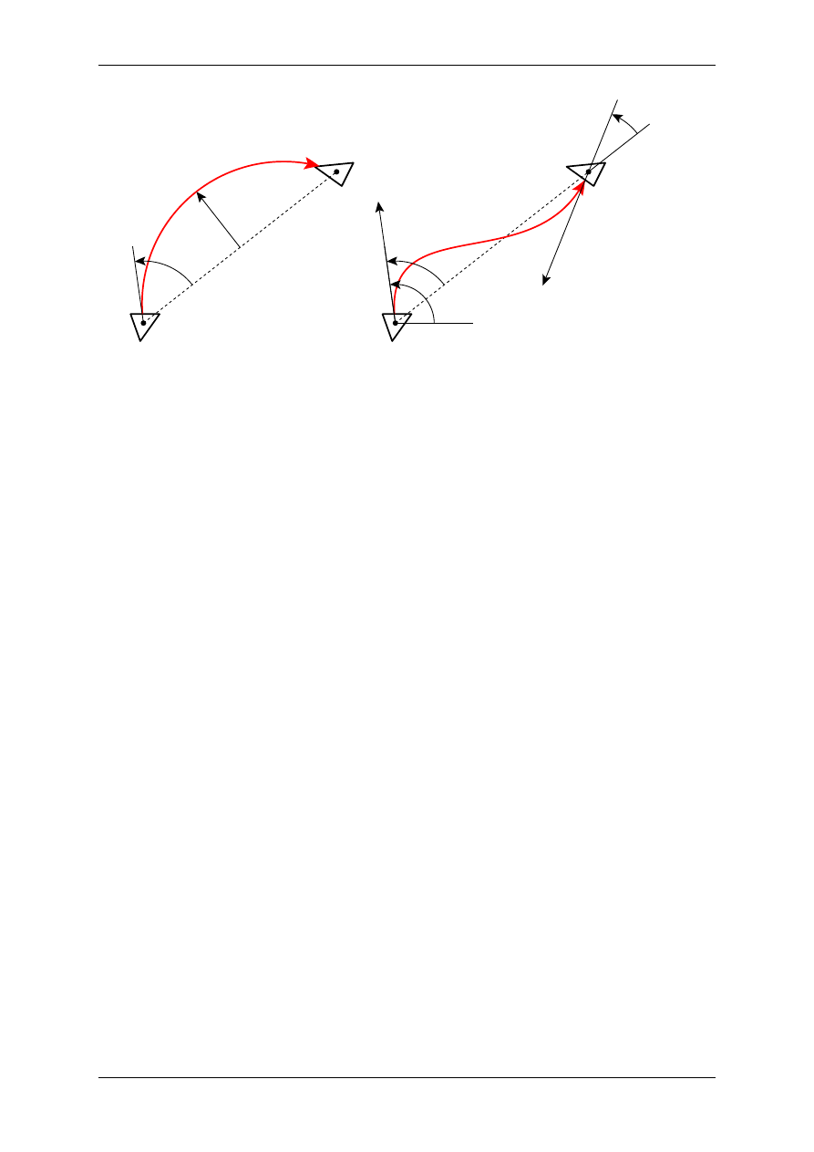
PyX Documentation, Release 0.11.1
relangle
(rel)bulge
relangle1
absangle1
relangle2
(rel)bulge
(rel)bulge
Figure 11.1: The angle-parameters of the connector.arc (left panel) and the connector.curve (right panel) classes.
11.4 Class twolines
This class returns two connected straight lines. There is a vast variety of combinations for angle- and length-
keywords. The user has to make sure to provide a non-ambiguous set of keywords:
absangle1
or relangle1 for the first angle, — relangleM for the middle angle and — absangle2 or relangle2 for
the ending angle. Again, the absolute angle overrides the relative if both are given. (Default: all five angles are
None
)
length1
and length2 for the lengths of the connecting lines. (Default: None)
60
Chapter 11. Module connector

CHAPTER
TWELVE
MODULE EPSFILE: EPS FILE
INCLUSION
With the help of the epsfile.epsfile class, you can easily embed another EPS file in your canvas, thereby
scaling, aligning the content at discretion. The most simple example looks like
from
pyx
import
*
c
=
canvas
.
canvas()
c
.
insert(epsfile
.
epsfile(
0
,
0
,
"file.eps"
))
c
.
writeEPSfile(
"output"
)
All relevant parameters are passed to the epsfile.epsfile constructor. They are summarized in the following
table:
argument
name
description
x
x-coordinate of position.
y
y-coordinate of position.
filename
Name of the EPS file (including a possible extension).
width=None
Desired width of EPS graphics or None for original width. Cannot be combined with scale
specification.
height=None
Desired height of EPS graphics or None for original height. Cannot be combined with scale
specification.
scale=None
Scaling factor for EPS graphics or None for no scaling. Cannot be combined with width or
height specification.
align="bl"
Alignment of EPS graphics. The first character specifies the vertical alignment: b for bottom,
c
for center, and t for top. The second character fixes the horizontal alignment: l for left, c
for center r for right.
clip=1
Clip to bounding box of EPS file?
translatebbox=1
Use lower left corner of bounding box of EPS file? Set to
0 with care.
bbox=None
If given, use bbox instance instead of bounding box of EPS file.
kpsearch=0
Search for file using the kpathsea library.
61

PyX Documentation, Release 0.11.1
62
Chapter 12. Module epsfile: EPS file inclusion

CHAPTER
THIRTEEN
BITMAPS
13.1 Introduction
PyX focuses on the creation of scaleable vector graphics. However, PyX also allows for the output of bitmap
images. Still, the support for creation and handling of bitmap images is quite limited. On the other hand the
interfaces are built that way, that its trivial to combine PyX with the “Python Image Library”, also known as
“PIL”.
The creation of a bitmap can be performed out of some unpacked binary data by first creating image instances:
from
pyx
import
*
image_bw
=
bitmap
.
image(
2
,
2
,
"L"
,
"\0\377\377\0"
)
image_rgb
=
bitmap
.
image(
3
,
2
,
"RGB"
,
"\77\77\77\177\177\177\277\277\277"
"\377\0\0\0\377\0\0\0\377"
)
Now image_bw is a
2 × 2 grayscale image. The bitmap data is provided by a string, which contains two
black ("\0" == chr(0)) and two white ("\377" == chr(255)) pixels. Currently the values per (colour)
channel is fixed to 8 bits. The coloured image image_rgb has
3 × 2 pixels containing a row of 3 different gray
values and a row of the three colours red, green, and blue.
The images can then be wrapped into bitmap instances by:
bitmap_bw
=
bitmap
.
bitmap(
0
,
1
, image_bw, height
=
0.8
)
bitmap_rgb
=
bitmap
.
bitmap(
0
,
0
, image_rgb, height
=
0.8
)
When constructing a bitmap instance you have to specify a certain position by the first two arguments fixing the
bitmaps lower left corner. Some optional arguments control further properties. Since in this example there is no
information about the dpi-value of the images, we have to specify at least a width or a height of the bitmap.
The bitmaps are now to be inserted into a canvas:
c
=
canvas
.
canvas()
c
.
insert(bitmap_bw)
c
.
insert(bitmap_rgb)
c
.
writeEPSfile(
"bitmap"
)
Figure
An introductory bitmap example.
shows the resulting output.
Figure 13.1: An introductory bitmap example.
63

PyX Documentation, Release 0.11.1
13.2 Bitmap module: Bitmap support
class bitmap.image(width, height, mode, data, compressed=None)
This class is a container for image data. width and height are the size of the image in pixel. mode is one
of "L", " RGB" or "CMYK" for grayscale, rgb, or cmyk colours, respectively. data is the bitmap data as
a string, where each single character represents a colour value with ordinal range 0 to 255. Each pixel is
described by the appropriate number of colour components according to mode. The pixels are listed row by
row one after the other starting at the upper left corner of the image.
compressed
might be set to " Flate" or "DCT" to provide already compressed data. Note that those data
will be passed to PostScript without further checks, i.e. this option is for experts only.
class bitmap.jpegimage(file)
This class is specialized to read data from a JPEG/JFIF-file. file is either an open file handle (it only has
to provide a read() method; the file should be opened in binary mode) or a string. In the latter case
will try to open a file named like file for reading.
The contents of the file is checked for some JPEG/JFIF format markers in order to identify the size and
dpi resolution of the image for further usage. These checks will typically fail for invalid data. The data
are not uncompressed, but directly inserted into the output stream (for invalid data the result will be invalid
PostScript). Thus there is no quality loss by recompressing the data as it would occur when recompressing
the uncompressed stream with the lossy jpeg compression method.
class bitmap.bitmap(xpos, ypos, image, width=None, height=None, ratio=None, storedata=0,
maxstrlen=4093
,
compressmode=”Flate”
,
flatecompresslevel=6
,
dctqual-
ity=75
, dctoptimize=1, dctprogression=0)
xpos
and ypos are the position of the lower left corner of the image. This position might be modified by
some additional transformations when inserting the bitmap into a canvas. image is an instance of
or
but it can also be an image instance from the “Python Image Library”.
width
, height, and ratio adjust the size of the image. At least width or height needs to be given, when no dpi
information is available from image.
storedata
is a flag indicating, that the (still compressed) image data should be put into the printers mem-
ory instead of writing it as a stream into the PostScript file. While this feature consumes memory of the
PostScript interpreter, it allows for multiple usage of the image without including the image data several
times in the PostScript file.
maxstrlen
defines a maximal string length when storedata is enabled. Since the data must be kept in the
PostScript interpreters memory, it is stored in strings. While most interpreters do not allow for an arbitrary
string length (a common limit is 65535 characters), a limit for the string length is set. When more data need
to be stored, a list of strings will be used. Note that lists are also subject to some implementation limits.
Since a typical value is 65535 entries, in combination a huge amount of memory can be used.
Valid values for compressmode currently are "Flate" (zlib compression), "DCT" (jpeg compression),
or None (disabling the compression). The zlib compression makes use of the zlib module as it is part of
the standard Python distribution. The jpeg compression is available for those image instances only, which
support the creation of a jpeg-compressed stream, e.g. images from the “Python Image Library” with jpeg
support installed. The compression must be disabled when the image data is already compressed.
flatecompresslevel
is a parameter of the zlib compression. dctquality, dctoptimize, and dctprogression are
parameters of the jpeg compression. Note, that the progression feature of the jpeg compression should be
turned off in order to produce valid PostScript. Also the optimization feature is known to produce errors on
certain printers.
64
Chapter 13. Bitmaps

CHAPTER
FOURTEEN
MODULE BBOX
The bbox‘ module contains the definition of the
class representing bounding boxes of graphical elements
like paths, canvases, etc. used in PyX. Usually, you obtain bbox instances as return values of the corresponding
bbox())
method, but you may also construct a bounding box by yourself.
14.1 bbox constructor
The bbox constructor accepts the following keyword arguments
keyword
description
llx
None
(default) for
−∞ or x-position of the lower left corner of the bbox (in user units)
lly
None
(default) for
−∞ or y-position of the lower left corner of the bbox (in user units)
urx
None
(default) for
∞ or x-position of the upper right corner of the bbox (in user units)
ury
None
(default) for
∞ or y-position of the upper right corner of the bbox (in user units)
14.2 bbox methods
bbox
method
function
intersects(other)
returns 1 if the bbox instance and other intersect with each other.
transformed(self, trafo)
returns self transformed by transformation trafo.
enlarged(all=0,
bottom=None, left=None,
top=None, right=None)
return the bounding box enlarged by the given amount (in visual
units). all is the default for all other directions, which is used
whenever None is given for the corresponding direction.
path()
or rect()
return the path corresponding to the bounding box rectangle.
height()
returns the height of the bounding box (in PyX lengths).
width()
returns the width of the bounding box (in PyX lengths).
top()
returns the
y-position of the top of the bounding box (in PyX
lengths).
bottom()
returns the
y-position of the bottom of the bounding box (in PyX
lengths).
left()
returns the
x-position of the left side of the bounding box (in PyX
lengths).
right()
returns the
x-position of the right side of the bounding box (in PyX
lengths).
Furthermore, two bounding boxes can be added (giving the bounding box enclosing both) and multiplied (giving
the intersection of both bounding boxes).
65

PyX Documentation, Release 0.11.1
66
Chapter 14. Module bbox

CHAPTER
FIFTEEN
MODULE COLOR
15.1 Color models
PostScript provides different color models. They are available to PyX by different color classes, which just pass
the colors down to the PostScript level. This implies, that there are no conversion routines between different color
models available. However, some color model conversion routines are included in Python’s standard library in the
module colorsym. Furthermore also the comparison of colors within a color model is not supported, but might
be added in future versions at least for checking color identity and for ordering gray colors.
There is a class for each of the supported color models, namely gray, rgb, cmyk, and hsb. The constructors
take variables appropriate for the color model. Additionally, a list of named colors is given in appendix
15.2 Example
from
pyx
import
*
c
=
canvas
.
canvas()
c
.
fill(path
.
rect(
0
,
0
,
7
,
3
), [color
.
gray(
0.8
)])
c
.
fill(path
.
rect(
1
,
1
,
1
,
1
), [color
.
rgb
.
red])
c
.
fill(path
.
rect(
3
,
1
,
1
,
1
), [color
.
rgb
.
green])
c
.
fill(path
.
rect(
5
,
1
,
1
,
1
), [color
.
rgb
.
blue])
c
.
writeEPSfile(
"color"
)
The file color.eps is created and looks like:
Figure 15.1: Color example
15.3 Color gradients
The color module provides a class gradient for continous transitions between colors. A list of named gradients
is available in appendix
67

PyX Documentation, Release 0.11.1
class color.gradient(min=0, max=1)
This class provides the methods for the gradient.
Different initializations can be found in
lineargradient
and functiongradient.
min
and max provide the valid range of the arguments for getcolor.
getcolor
(
parameter)
Returns the color that corresponds to parameter (must be between min and max).
select
(
index
, n_indices)
When a total number of n_indices different colors is needed from the gradient, this method returns the
index
-th color.
class color.lineargradient(startcolor, endcolor, min=0, max=1)
This class provides a linear transition between two given colors. The linear interpolation is performed on
the color components of the specific color model.
startcolor
and endcolor must be colors of the same color model.
class color.functiongradient(functions, type, min=0, max=1)
This class provides an arbitray transition between colors of the same color model.
type
is a string indicating the color model (one of "cmyk", "rgb", "hsb", "grey")
functions
is a dictionary that maps the color components onto given functions. E.g. for type="rgb" this
dictionary must have the keys "r", "g", and "b".
15.4 Transparency
class color.transparency(value)
Instances of this class will make drawing operations (stroking, filling) to become partially transparent. value
defines the transparency factor in the range 0 (opaque) to 1 (transparent).
Transparency is available in PDF output only since it is not supported by PostScript. However, for certain
ghostscript devices (for example the pdf backend as used by ps2pdf) proprietary PostScript extension allows
for transparency in PostScript code too. PyX creates such PostScript proprietary code, but issues a warning
when doing so.
68
Chapter 15. Module color

CHAPTER
SIXTEEN
MODULE PATTERN
This module contains the
class, whichs allows the definition of PostScript Tiling patterns (cf. Sect. 4.9
of the PostScript Language Reference Manual) which may then be used to fill paths. In addition, a number of
predefined hatch patterns are included.
16.1 Class pattern
The classes
and
differ only in their constructor and in the absence of a writeEPSfile()
method in the former. The
constructor accepts the following keyword arguments:
key-
word
description
painttype1
(default) for coloured patterns or 2 for uncoloured patterns
tilingtype
1
(default) for constant spacing tilings (patterns are spaced constantly by a multiple of a device
pixel), 2 for undistorted pattern cell, whereby the spacing may vary by as much as one device
pixel, or 3 for constant spacing and faster tiling which behaves as tiling type 1 but with
additional distortion allowed to permit a more efficient implementation.
xstep
desired horizontal spacing between pattern cells, use None (default) for automatic calculation
from pattern bounding box.
ystep
desired vertical spacing between pattern cells, use None (default) for automatic calculation from
pattern bounding box.
bbox
bounding box of pattern. Use None for an automatic determination of the bounding box
(including an enlargement by bboxenlarge pts on each side.)
trafo
additional transformation applied to pattern or None (default). This may be used to rotate the
pattern or to shift its phase (by a translation).
bboxenlarge
enlargement when using the automatic bounding box determination; default is 5 pts.
After you have created a pattern instance, you define the pattern shape by drawing in it like in an ordinary canvas.
To use the pattern, you simply pass the pattern instance to a stroke(), fill(), draw() or set() method
of the canvas, just like you would do with a colour, etc.
69

PyX Documentation, Release 0.11.1
70
Chapter 16. Module pattern

CHAPTER
SEVENTEEN
MODULE UNIT
With the unit module PyX makes available classes and functions for the specification and manipulation of
lengths. As usual, lengths consist of a number together with a measurement unit, e.g., 1 cm, 50 points, 0.42 inch.
In addition, lengths in PyX are composed of the five types “true”, “user”, “visual”, “width”, and “TeX”, e.g., 1
user cm, 50 true points, 0.42 visual + 0.2 width inch. As their names indicate, they serve different purposes. True
lengths are not scalable and are mainly used for return values of PyX functions. The other length types can be
rescaled by the user and differ with respect to the type of object they are applied to:
user length: used for lengths of graphical objects like positions etc.
visual length: used for sizes of visual elements, like arrows, graph symbols, axis ticks, etc.
width length: used for line widths
TeX length: used for all TeX and LaTeX output
When not specified otherwise, all types of lengths are interpreted in terms of a default unit, which, by default, is 1
cm. You may change this default unit by using the module level function
unit.set(
uscale=None
, vscale=None, wscale=None, xscale=None, defaultunit=None)
When uscale, vscale, wscale, or xscale is not None, the corresponding scaling factor(s) is redefined to the
given number. When defaultunit is not None, the default unit is set to the given value, which has to be one
of "cm", "mm", "inch", or "pt".
For instance, if you only want thicker lines for a publication version of your figure, you can just rescale all width
lengths using
unit
.
set(wscale
=
2
)
Or suppose, you are used to specify length in imperial units. In this, admittedly rather unfortunate case, just use
unit
.
set(defaultunit
=
"inch"
)
at the beginning of your program.
17.1 Class length
class unit.length(f, type=”u”, unit=None)
The constructor of the
class expects as its first argument a number f, which represents the prefactor
of the given length. By default this length is interpreted as a user length (type="u") in units of the current
default unit (see
function of the
module). Optionally, a different type may be specified,
namely "u" for user lengths, "v" for visual lengths, "w" for width lengths, "x" for TeX length, and "t"
for true lengths. Furthermore, a different unit may be specified using the unit argument. Allowed values are
"cm"
, "mm", "inch", and "pt".
Instances of the
class support addition and substraction either by another
or by a number which
is then interpeted as being a user length in default units, multiplication by a number and division either by another
in which case a float is returned or by a number in which case a
instance is returned. When two
71
PyX Documentation, Release 0.11.1
lengths are compared, they are first converted to meters (using the currently set scaling), and then the resulting
values are compared.
17.2 Predefined length instances
A number of length instances are already predefined, which only differ in there values for type and unit.
They are summarized in the following table
name
type
unit
m
user
m
cm
user
cm
mm
user
mm
inch
user
inch
pt
user
points
t_m
true
m
t_cm
true
cm
t_mm
true
mm
t_inch
true
inch
t_pt
true
points
u_m
user
m
u_cm
user
cm
u_mm
user
mm
u_inch
user
inch
u_pt
user
points
v_m
visual
m
v_cm
visual
cm
v_mm
visual
mm
v_inch
visual
inch
v_pt
visual
points
w_m
width
m
w_cm
width
cm
w_mm
width
mm
w_inch
width
inch
w_pt
width
points
x_m
TeX
m
x_cm
TeX
cm
x_mm
TeX
mm
x_inch
TeX
inch
x_pt
TeX
points
Thus, in order to specify, e.g., a length of 5 width points, just use 5*unit.w_pt.
17.3 Conversion functions
If you want to know the value of a PyX length in certain units, you may use the predefined conversion functions
which are given in the following table
function
result
tom(l)
l
in units of m
tocm(l)
l
in units of cm
tomm(l)
l
in units of mm
toinch(l)
l
in units of inch
topt(l)
l
in units of points
If l is not yet a length instance but a number, it first is interpreted as a user length in the default units.
72
Chapter 17. Module unit

CHAPTER
EIGHTEEN
MODULE TRAFO: LINEAR
TRANSFORMATIONS
With the trafo module PyX supports linear transformations, which can then be applied to canvases, Bézier paths
and other objects. It consists of the main class trafo representing a general linear transformation and subclasses
thereof, which provide special operations like translation, rotation, scaling, and mirroring.
18.1 Class trafo
The trafo class represents a general linear transformation, which is defined for a vector
~x as
XXX: translate this math
\vec{x}’ = \mathsf{A}\, \vec{x} + \vec{b}\ ,
where A is the transformation matrix and ~
b the translation vector. The transformation matrix must not be singular,
i.e.
we require
det A 6= 0.
Multiple trafo instances can be multiplied, corresponding to a consecutive application of the respective transfor-
mation. Note that trafo1*trafo2 means that trafo1 is applied after trafo2, i.e. the new transformation
is given by A
= A
1
A
2
and ~
b = A
1
~b
2
+ ~b
1
. Use the trafo methods described below, if you prefer thinking the
other way round. The inverse of a transformation can be obtained via the trafo method inverse(), defined
by the inverse A
−1
of the transformation matrix and the translation vector
−A
−1
~b.
The methods of the trafo class are summarized in the following table.
trafo
method
function
__init__(matrix=((1,0),(0,1)),
vector=(0,0)):
create new trafo instance with transformation matrix and vector.
apply(x, y)
apply trafo to point vector
(x, y).
inverse()
returns inverse transformation of trafo.
mirrored(angle)
returns trafo followed by mirroring at line through
(0, 0) with direction
angle
in degrees.
rotated(angle,
x=None, y=None)
returns trafo followed by rotation by angle degrees around point
(x, y),
or
(0, 0), if not given.
scaled(sx, sy=None,
x=None, y=None)
returns trafo followed by scaling with scaling factor sx in
x-direction,
sy
in
y-direction (sy = sx, if not given) with scaling center (x, y), or
(0, 0), if not given.
translated(x, y)
returns trafo followed by translation by vector
(x, y).
slanted(a, angle=0,
x=None, y=None)
returns trafo followed by XXX
73

PyX Documentation, Release 0.11.1
18.2 Subclasses of trafo
The trafo module provides a number of subclasses of the trafo class, each of which corresponds to one
trafo
method. They are listed in the following table:
trafo
subclass
function
mirror(angle)
mirroring at line through
(0, 0) with direction angle in degrees.
rotate(angle,
x=None, y=None)
rotation by angle degrees around point
(x, y), or (0, 0), if not given.
scale(sx, sy=None,
x=None, y=None)
scaling with scaling factor sx in
x-direction, sy in y-direction (sy = sx, if
not given) with scaling center
(x, y), or (0, 0), if not given.
translate(x, y)
translation by vector
(x, y).
slant(a, angle=0,
x=None, y=None)
XXX
74
Chapter 18. Module trafo: Linear transformations
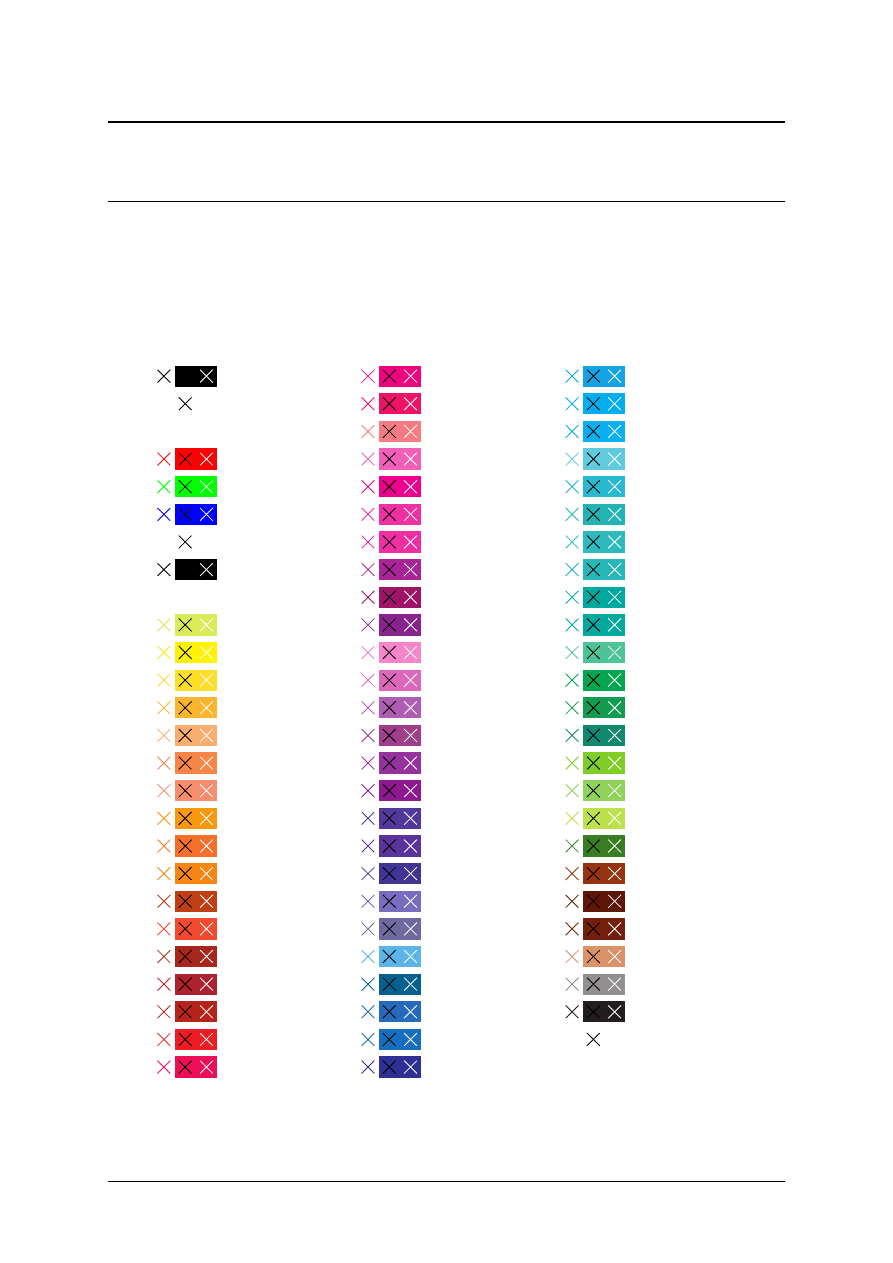
CHAPTER
NINETEEN
APPENDIX: NAMED COLORS
grey.black
grey.white
rgb.red
rgb.green
rgb.blue
rgb.white
rgb.black
cmyk.GreenYellow
cmyk.Yellow
cmyk.Goldenrod
cmyk.Dandelion
cmyk.Apricot
cmyk.Peach
cmyk.Melon
cmyk.YellowOrange
cmyk.Orange
cmyk.BurntOrange
cmyk.Bittersweet
cmyk.RedOrange
cmyk.Mahogany
cmyk.Maroon
cmyk.BrickRed
cmyk.Red
cmyk.OrangeRed
cmyk.RubineRed
cmyk.WildStrawberry
cmyk.Salmon
cmyk.CarnationPink
cmyk.Magenta
cmyk.VioletRed
cmyk.Rhodamine
cmyk.Mulberry
cmyk.RedViolet
cmyk.Fuchsia
cmyk.Lavender
cmyk.Thistle
cmyk.Orchid
cmyk.DarkOrchid
cmyk.Purple
cmyk.Plum
cmyk.Violet
cmyk.RoyalPurple
cmyk.BlueViolet
cmyk.Periwinkle
cmyk.CadetBlue
cmyk.CornflowerBlue
cmyk.MidnightBlue
cmyk.NavyBlue
cmyk.RoyalBlue
cmyk.Blue
cmyk.Cerulean
cmyk.Cyan
cmyk.ProcessBlue
cmyk.SkyBlue
cmyk.Turquoise
cmyk.TealBlue
cmyk.Aquamarine
cmyk.BlueGreen
cmyk.Emerald
cmyk.JungleGreen
cmyk.SeaGreen
cmyk.Green
cmyk.ForestGreen
cmyk.PineGreen
cmyk.LimeGreen
cmyk.YellowGreen
cmyk.SpringGreen
cmyk.OliveGreen
cmyk.RawSienna
cmyk.Sepia
cmyk.Brown
cmyk.Tan
cmyk.Gray
cmyk.Black
cmyk.White
Figure 19.1: Names colors
75

PyX Documentation, Release 0.11.1
76
Chapter 19. Appendix: Named colors
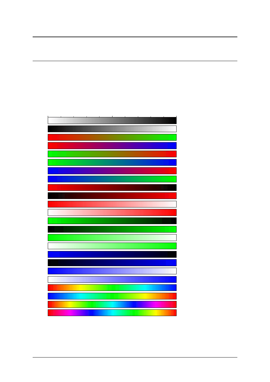
CHAPTER
TWENTY
APPENDIX: NAMED GRADIENTS
0
1
gradient.Gray
gradient.ReverseGray
gradient.RedGreen
gradient.RedBlue
gradient.GreenRed
gradient.GreenBlue
gradient.BlueRed
gradient.BlueGreen
gradient.RedBlack
gradient.BlackRed
gradient.RedWhite
gradient.WhiteRed
gradient.GreenBlack
gradient.BlackGreen
gradient.GreenWhite
gradient.WhiteGreen
gradient.BlueBlack
gradient.BlackBlue
gradient.BlueWhite
gradient.WhiteBlue
gradient.Rainbow
gradient.ReverseRainbow
gradient.Hue
gradient.ReverseHue
Figure 20.1: Names gradients
77

PyX Documentation, Release 0.11.1
78
Chapter 20. Appendix: Named gradients
CHAPTER
TWENTYONE
APPENDIX: PATH STYLES
linecap.butt
(default)
linecap.round
linecap.square
linejoin.miter
(default)
linejoin.round
linejoin.bevel
linestyle.solid
(default)
linestyle.dashed
linestyle.dotted
linestyle.dashdotted
linewidth.THIN
linewidth.THIn
linewidth.THin
linewidth.Thin
linewidth.thin
linewidth.normal
(default)
linewidth.thick
linewidth.Thick
linewidth.THick
linewidth.THIck
linewidth.THICk
linewidth.THICK
miterlimit.lessthan180deg
miterlimit.lessthan90deg
miterlimit.lessthan60deg
miterlimit.lessthan45deg
miterlimit.lessthan11deg
(default)
dash((1, 1, 2, 2, 3, 3), 0)
dash((1, 1, 2, 2, 3, 3), 1)
dash((1, 2, 3), 2)
dash((1, 2, 3), 3)
dash((1, 2, 3), 4)
dash((1, 2, 3), rellengths=1)
Figure 21.1: path styles
79

PyX Documentation, Release 0.11.1
80
Chapter 21. Appendix: path styles
CHAPTER
TWENTYTWO
APPENDIX: ARROWS IN DECO
MODULE
earrow.Small
earrow.small
earrow.normal
earrow.large
earrow.Large
barrow.normal
earrow.Large([deco.filled([color.rgb.red]), style.linewidth.normal])
earrow.normal(constriction=None)
earrow.Large([style.linejoin.round])
earrow.Large([deco.stroked.clear])
Figure 22.1: Arrows in deco module
81

PyX Documentation, Release 0.11.1
82
Chapter 22. Appendix: Arrows in deco module

PYTHON MODULE INDEX
b
bbox
,
bitmap
,
box
,
c
canvas
,
color
,
connector
,
d
deformer
,
document
,
e
epsfile
,
g
graph
,
graph.axis
,
graph.axis.axis
,
graph.axis.painter
,
graph.axis.parter
,
graph.axis.positioners
,
graph.axis.rater
,
graph.axis.texter
,
graph.axis.tick
,
graph.data
,
graph.graph
,
graph.key
,
graph.style
,
p
path
,
pattern
,
s
style
,
t
text
,
trafo
,
u
unit
,
83

PyX Documentation, Release 0.11.1
84
Python Module Index

INDEX
Symbols
__call__() (deformer.deformer method),
A
allwarning (text.texmessage attribute),
anchoredaxis (class in graph.axis.axis),
anchoredpathaxis (class in graph.axis.axis),
append() (path.normsubpath method),
append() (path.path method),
arc (class in path),
arclen() (path.path method),
arclentoparam() (path.path method),
arcn (class in path),
arct (class in path),
arrow (class in graph.style),
at() (path.path method),
atbegin() (path.path method),
atend() (path.path method),
autolin (class in graph.axis.parter),
autolinear (class in graph.axis.parter),
autolog (class in graph.axis.parter),
autologarithmic (class in graph.axis.parter),
axes (graph.graph.graphxy attribute),
axisatv() (graph.graph.graphxy method),
axistrafo() (graph.graph.graphxy method),
B
bar (class in graph.axis.axis),
bar (class in graph.axis.painter),
bar (class in graph.style),
barpos (class in graph.style),
baseline (text.valign attribute),
basepath() (graph.axis.axis.anchoredaxis method),
bbox (module),
bbox() (canvas.canvas method),
bbox() (path.path method),
begin() (path.path method),
bitmap (class in bitmap),
bitmap (module),
bottom (text.valign attribute),
bottomzero (text.vshift attribute),
box (module),
boxcenter (text.halign attribute),
boxleft (text.halign attribute),
boxright (text.halign attribute),
boxwarning (text.texmessage attribute),
C
canvas (class in canvas),
canvas (module),
cbdfile (class in graph.data),
center (text.halign attribute),
central (class in graph.graph),
central (graph.graph.graphxyz attribute),
changebar (class in graph.style),
changecircle (graph.style.symbol attribute),
changecircletwice (graph.style.symbol attribute),
changecross (graph.style.symbol attribute),
changediamond (graph.style.symbol attribute),
changediamondtwice (graph.style.symbol attribute),
changefilledstroked (graph.style.symbol attribute),
changelinestyle (graph.style.line attribute),
changeplus (graph.style.symbol attribute),
changesquare (graph.style.symbol attribute),
changesquaretwice (graph.style.symbol attribute),
changestrokedfilled (graph.style.symbol attribute),
changetriangle (graph.style.symbol attribute),
changetriangletwice (graph.style.symbol attribute),
circle (class in path),
circle (graph.style.symbol attribute),
close() (path.normsubpath method),
closepath (class in path),
color (module),
conffile (class in graph.data),
connector (module),
cross (graph.style.symbol attribute),
cube (class in graph.axis.rater),
curve (class in path),
curveradius() (path.path method),
curveto (class in path),
cycloid (class in deformer),
D
data (class in graph.data),
decimal (class in graph.axis.texter),
defaultcolumnpattern (graph.data.file attribute),
defaultcommentpattern (graph.data.file attribute),
defaultstringpattern (graph.data.file attribute),
defaulttexrunner (in module text),
defaultvariants (graph.axis.parter.autolinear attribute),
85

PyX Documentation, Release 0.11.1
defaultvariants (graph.axis.parter.autologarithmic at-
tribute),
deform() (deformer.deformer method),
deformer (class in deformer),
deformer (module),
diamond (graph.style.symbol attribute),
distance (class in graph.axis.rater),
doaxes() (graph.graph.graphxy method),
dobackground() (graph.graph.graphxy method),
document (class in document),
document (module),
dokey() (graph.graph.graphxy method),
dokeyitem() (graph.graph.graphxy method),
dolayout() (graph.graph.graphxy method),
doplot() (graph.graph.graphxy method),
doplotitem() (graph.graph.graphxy method),
draw() (canvas.canvas method),
E
end (text.texmessage attribute),
end() (path.path method),
epsfile (module),
errorbar (class in graph.style),
exponential (class in graph.axis.texter),
extend() (path.normsubpath method),
extend() (path.path method),
F
file (class in graph.data),
fill() (canvas.canvas method),
finish() (graph.graph.graphxy method),
flushcenter (text.halign attribute),
flushleft (text.halign attribute),
flushright (text.halign attribute),
fontwarning (text.texmessage attribute),
footnotesize (text.size attribute),
function (class in graph.data),
functiongradient (class in color),
G
gradient (class in color),
gradient.getcolor() (in module color),
gradient.select() (in module color),
graph (module),
graph.axis (module),
graph.axis.axis (module),
graph.axis.painter (module),
graph.axis.parter (module),
graph.axis.positioners (module),
graph.axis.rater (module),
graph.axis.texter (module),
graph.axis.tick (module),
graph.data (module),
graph.graph (module),
graph.key (module),
graph.style (module),
graphicsload (text.texmessage attribute),
graphxy (class in graph.graph),
graphxyz (class in graph.graph),
grid (class in graph.style),
gridpath() (graph.axis.axis.anchoredaxis method),
gridpos (class in graph.style),
H
halign (class in text),
histogram (class in graph.style),
Huge (text.size attribute),
huge (text.size attribute),
I
ignore (text.texmessage attribute),
image (class in bitmap),
impulses (class in graph.style),
insert() (canvas.canvas method),
intersect() (path.path method),
J
join() (path.normpath method),
joined() (path.path method),
jpegimage (class in bitmap),
K
key (class in graph.key),
L
LARGE (text.size attribute),
Large (text.size attribute),
large (text.size attribute),
left (text.halign attribute),
length (class in unit),
lin (class in graph.axis.axis),
lin (class in graph.axis.parter),
lin (class in graph.axis.rater),
line (class in graph.style),
line (class in path),
linear (class in graph.axis.axis),
linear (class in graph.axis.parter),
linear (class in graph.axis.rater),
lineargradient (class in color),
lineto (class in path),
linked (class in graph.axis.painter),
linkedaxis (class in graph.axis.axis),
linkedbar (class in graph.axis.painter),
linkedsplit (class in graph.axis.painter),
load (text.texmessage attribute),
loaddef (text.texmessage attribute),
log (class in graph.axis.axis),
log (class in graph.axis.parter),
log (class in graph.axis.rater),
logarithmic (class in graph.axis.axis),
logarithmic (class in graph.axis.parter),
logarithmic (class in graph.axis.rater),
M
mathaxis (text.vshift attribute),
86
Index

PyX Documentation, Release 0.11.1
mathmode (in module text),
middle (text.valign attribute),
middlezero (text.vshift attribute),
mixed (class in graph.axis.texter),
moveto (class in path),
multicurveto_pt (class in path),
multilineto_pt (class in path),
N
nestedbar (class in graph.axis.axis),
noaux (text.texmessage attribute),
normalsize (text.size attribute),
normpath (class in path),
normpath() (path.path method),
normsubpath (class in path),
O
orthogonal (graph.axis.painter.rotatetext attribute),
P
page (class in document),
paperformat (class in document),
parallel (class in deformer),
parallel (class in graph.graph),
parallel (graph.axis.painter.rotatetext attribute),
parallel (graph.graph.graphxyz attribute),
paramfunction (class in graph.data),
paramtoarclen() (path.path method),
parbox (class in text),
path (class in path),
path (module),
pattern (module),
phantom (in module text),
pipeGS() (canvas.canvas method),
plot() (graph.graph.graphxy method),
plus (graph.style.symbol attribute),
points (class in graph.data),
pos (class in graph.style),
pos() (graph.graph.graphxy method),
positioner (class in graph.axis.positioners),
pre125exp (graph.axis.parter.logarithmic attribute),
pre1exp (graph.axis.parter.logarithmic attribute),
pre1exp2 (graph.axis.parter.logarithmic attribute),
pre1exp3 (graph.axis.parter.logarithmic attribute),
pre1exp4 (graph.axis.parter.logarithmic attribute),
pre1exp5 (graph.axis.parter.logarithmic attribute),
pre1to9exp (graph.axis.parter.logarithmic attribute),
preamble() (in module text),
preamble() (text.texrunner method),
preexp (class in graph.axis.parter),
R
raggedcenter (text.halign attribute),
raggedleft (text.halign attribute),
raggedright (text.halign attribute),
range (class in graph.style),
range() (path.path method),
rater (class in graph.axis.rater),
rational (class in graph.axis.texter),
rational (class in graph.axis.tick),
rcurveto (class in path),
rect (class in graph.style),
rect (class in path),
regular (class in graph.axis.painter),
reset() (in module text),
reset() (text.texrunner method),
reverse() (path.normpath method),
reversed() (path.path method),
right (text.halign attribute),
rlineto (class in path),
rmoveto (class in path),
rotatetext (class in graph.axis.painter),
rotation() (path.path method),
S
scriptsize (text.size attribute),
set() (in module text),
set() (in module unit),
set() (text.texrunner method),
setlinkedaxis() (graph.axis.axis.linkedaxis method),
settexrunner() (canvas.canvas method),
size (class in text),
small (text.size attribute),
smoothed (class in deformer),
split (class in graph.axis.axis),
split (class in graph.axis.painter),
split() (path.path method),
splitatvalue() (in module graph.data),
square (graph.style.symbol attribute),
stackedbarpos (class in graph.style),
start (text.texmessage attribute),
stroke() (canvas.canvas method),
style (module),
surface (class in graph.style),
symbol (class in graph.style),
T
tangent() (path.path method),
texmessage (class in text),
texmessagepattern (class in text),
texrunner (class in text),
text (class in graph.style),
text (module),
text() (canvas.canvas method),
text() (in module text),
text() (text.texrunner method),
tick (class in graph.axis.tick),
tickdirection() (graph.axis.axis.anchoredaxis method),
ticklength (class in graph.axis.painter),
tickpoint() (graph.axis.axis.anchoredaxis method),
tiny (text.size attribute),
top (text.valign attribute),
topzero (text.vshift attribute),
trafo (module),
trafo() (path.path method),
Index
87

PyX Documentation, Release 0.11.1
transform() (path.normpath method),
transformed() (path.path method),
transparency (class in color),
triangle (graph.style.symbol attribute),
U
unit (module),
V
valign (class in text),
values (class in graph.data),
vangle() (graph.graph.graphxyz method),
vbasepath() (graph.axis.axis.anchoredaxis method),
vbasepath() (graph.axis.positioners.positioner method),
vgeodesic() (graph.graph.graphxy method),
vgeodesic_el() (graph.graph.graphxy method),
vgridpath() (graph.axis.axis.anchoredaxis method),
vgridpath() (graph.axis.positioners.positioner method),
vpos() (graph.graph.graphxy method),
vshift (class in text),
vtickdirection() (graph.axis.axis.anchoredaxis method),
vtickdirection()
(graph.axis.positioners.positioner
method),
vtickpoint() (graph.axis.axis.anchoredaxis method),
vtickpoint_pt()
(graph.axis.positioners.positioner
method),
vzindex() (graph.graph.graphxyz method),
W
writeEPSfile() (canvas.canvas method),
writeEPSfile() (document.document method),
writePDFfile() (canvas.canvas method),
writePDFfile() (document.document method),
writePSfile() (canvas.canvas method),
writePSfile() (document.document method),
writetofile() (canvas.canvas method),
writetofile() (document.document method),
X
xbasepath() (graphxy method),
xgridpath() (graphxy method),
xtickdirection() (graphxy method),
xtickpoint() (graphxy method),
xvbasepath() (graphxy method),
xvgridpath() (graphxy method),
xvtickdirection() (graphxy method),
xvtickpoint() (graphxy method),
Y
ybasepath() (graphxy method),
ygridpath() (graphxy method),
ytickdirection() (graphxy method),
ytickpoint() (graphxy method),
yvbasepath() (graphxy method),
yvgridpath() (graphxy method),
yvtickdirection() (graphxy method),
yvtickpoint() (graphxy method),
88
Index
Document Outline
- Introduction
- Basic graphics
- Module path
- Module deformer: Path deformers
- Module canvas
- Module document
- Module text: TeX/LaTeX interface
- Graphs
- Axes
- Module box: Convex box handling
- Module connector
- Module epsfile: EPS file inclusion
- Bitmaps
- Module bbox
- Module color
- Module pattern
- Module unit
- Module trafo: Linear transformations
- Appendix: Named colors
- Appendix: Named gradients
- Appendix: path styles
- Appendix: Arrows in deco module
- Python Module Index
- Index
Wyszukiwarka
Podobne podstrony:
Manual do zadania 2010 03
Manual do exam
Manual do concurseiro 9ª edição Alexandre Meirelles
Paulo Coelho 1997 – O Manual do Guerreiro da Luz
Instrukcja do karabinu M16 OPERATOR MANUAL M16 AND M16A1
Paulo Coelho 1986 – O Manual Prático do Vampirismo
Test do badania poziomu sprawności manualnej i percepcji wzrokowej H. Spionek
tab. pom. do sprawności manualnej, ćwiczenia, karty pracy
Medycyna manualna Wprowadzenie do teorii, rozpoznawanie i leczeni Dr H D Neumann
Przybory i przyrz±dy do æwiczeñ manualnych
mapy do celow proj
Seminarium IIIR do kopiowania
Szkol Wykład do Or
ROS wykorzystanie roslin do unieszkodliwiania osadow
Środki miejscowo znieczulające i do znieczulenia ogólnego(1)
Bakterie spiralne do druk
więcej podobnych podstron