Duration Analysis in the Australian
Coal Industry

Anthony B. Lawrance *
Robert E. Marks *

Working Paper 00–008
April 2000.

We are grateful for the generous help from Tom Callcott, Ruth Callcott and Glen Barnett. We
also acknowledge the assistance of the Joint Coal Board chairman, Ian Farrer, the statistician
Carol Mische, and other staff, in providing access to records, without which we could not have
constructed the data base.

Working Papers are a series of manuscripts in their draft form. They are not intended for
circulation or distribution except as indicated by the author. For that reason Working Papers
may not be quoted, reproduced or distributed without the written consent of the author.

*

Australian Graduate School of Management, University of New South Wales, Sydney
NSW 2052, Australia.

ISBN 1 86274 376 2

1

DURATION ANALYSIS IN THE AUSTRALIAN COAL INDUSTRY

1

Anthony B Lawrance

Robert E Marks

Australian Graduate School of Management

UNSW, SYDNEY, NSW 2052

Australia

[e-mail]

[e-mail]

March 29, 2000

Abstract

Previous duration studies have not identified all entry and exit dates, have used some

aggregated data, and have lacked complete information on mergers and acquisitions. We

determine the durations of Australian coal-producing companies over a forty-year period,

having constructed a clean database describing the 85 companies. We fit a Weibull

distribution to the Kaplan-Meier product limit estimator results and use maximum likelihood

estimators as parameters. Unlike studies of manufacturing companies, we find, first, that

survival decreases with age, second, no relation between size and survival, and, third,

evidence of an increase in the characteristic life over the period.

JEL Classifications: C41, L11, L71

1

We are grateful for the generous help from Tom Callcott, Ruth Callcott and Glen Barnett. We also

acknowledge the assistance of the Joint Coal Board chairman, Ian Farrer, the statistician Carol Mische,
and other staff, in providing access to records, without which we could not have constructed the data
base.

2

I Introduction

The use of statistical analysis of life cycles has long been established in engineering and the

bio-medical fields (see J.D. Kalbfleisch and R.L. Prentice (1980) for bibliographical

treatment) and was introduced into economics in the 1970s in the analysis of strikes and

unemployment (Tony Lancaster 1979) and, later, in analysis of the survival of firms (David

B. Audretsch 1991; Audretsch and Talat Mahmood 1995; Timothy Dunne, Mark J. Roberts,

and Larry Samuelson 1989; David S. Evans 1987a; Rajshree Agarwal, 1997), although much

of the work is more related to growth and the testing of Gibrat's Law of proportional growth

than to the duration of firms. "Survival of firms has ... been studied as a side issue to growth

of firms" (Agarwal 1997)

Audretsch and Mahmood found that "One of the most striking stylized facts regarding the

dynamics of industries, that has emerged from empirical studies, is that the survival rates of

businesses are positively related both to establishment size and age" (Audretsch and

Mahmood 1995, p.97). This is also evidenced by the work of Dunne, Roberts, and Samuelson

(1989); and Evans (1987a). The work of Agarwal "confirms Jovanovic's hypothesis [Boyan

Jovanovic 1982] that survival increases with size" (Agarwal 1997, p.580).

We analyze the duration of NSW coal companies from 1960 to 1999 and test the relation of

duration to size and age. Australia is the world's largest exporter of coal, overtaking the USA

in 1984 (IEA/OECD 1999) and coal is Australia's largest export earner (McLennan 1999)

with New South Wales (NSW) and Queensland being the exporting regions . While

Queensland has now exceeded NSW in exports (JCB 1999), NSW has a longer history of

substantial coal mining and exports, and our analysis is centered on NSW. From 1960 to

3

1998 NSW coal production rose from 16 million tonnes to 108 million tonnes and exports

rose from 1 million tonnes to 76 million tonnes (Tex Report various).

Because coal companies depend on coal reserves, which decline with extraction, we

hypothesize survival rates to be negatively related to age (ceteris paribus). Because large

companies extract coal at higher rates than small companies (our definition of size is the

annual production or extraction rate), again we expect survival rates (cet. par.) to be

negatively related to size. Some aspects which would void the ceteris paribus assumption,

could be the introduction of new technology, which allows economic mining at greater

depths, and the acquisition of additional reserves, either by new grants by the Government or

by purchase from other operators. Moreover, our definition of the size of an operator is its

total production, and not the production from individual mine sites. The relation between size

of operator and reduction of total reserves for a large operator will not necessarily be greater

than that of a small operator, which may be reducing its reserves from a small mine at the

same or a greater rate.

While there have been a number of papers on the duration of manufacturing companies,

(Dunne, Roberts, and Samuelson 1988; Dunne, Roberts, and Samuelson 1989; Audretsch

1991; Audretsch and Mahmood 1995) we have found none on mining companies and

certainly no published analysis of duration in the Australian coal industry.

There has been considerable interest recently in the demise of Australian companies and their

failure to pay the employees their full entitlements. A notable recent example was that of the

failure of the Oakdale coal company, which caused the Australian Government to call on the

4

industry to pay the workers' entitlements from the industry long-service leave fund (SMH

1999), and so an analysis of the life times of coal companies would seem timely.

We define the "death" of a company (an "operator"), or "finish" of its life, by the date at

which the company no longer has a controlling interest in a coal operation. Despite the

concern of events such as Oakdale, which went into receivership, this form of finish is not the

norm. Frequently, the legal corporate entity continues, but with new owners. We therefore

take the ultimate majority, or managing, shareholder as the "operator" and analyze its entry

into ("start"), and departure from ("finish"), the industry, in a position of controlling some

coal production. Where the company shares of an operator are broadly held, with no

dominant shareholder, we consider the company itself to be the operator. We also trace

ownership to the ultimate controlling owner; we do necessarily not stop at the first legal entity

which is a direct owner of the coal mine. A number of companies manage their mines under

subsidiary companies and, failure to identify the ultimate owner, would give a completely

misleading picture of the industry. We are not concerned with individual mines and, provided

an operator maintains a controlling interest in at least one coal mine, its status does not alter

in this duration analysis if one or more of its mines close, or are otherwise disposed of.

II Empirical data

In our analysis we use "single spell" or "survival" stock sampling data from the Joint Coal

Board (JCB) records and other sources These data provide a list of operating companies, their

controlling shareholder and the dates at which this shareholder gained or lost control of its

5

coal operations. The method of construction of the data base, and its sources, is given in

Appendix 5

2

.

We define "start" as the first occasion that an operator produced coal, or the date at which the

operator's first mine opened, if it achieved at least 100,000 tonnes of production in the first

twelve months of operation; otherwise we use the start of the financial year (July 1 to June

30) in which 100,000 tonnes production was first achieved

3

. For "finish" date, we use the

date of sale of the last coal mine owned by the operator or the date of change of control of the

coal mines, or of the operator itself (in some cases this was the date of start of liquidation

proceedings). Where only the month of start or finish is known, we use the first of the month.

Where more than one operator has the same duration in days, we change the start date by one

day—we consider this appropriate as the "correct" start date is an uncertain time and this

change makes the statistical analysis easier

4

. Many analyses by other authors have been

hampered by the difficulty of identifying entry and exit dates (Audretsch and Mahmood

1995), by aggregated data which does not reveal individual firms (Audretsch 1991) and by

lack of data on mergers and acquisitions (Evans 1987b), but our data reveal the direct

majority ownership and identify entry and exit with reasonable accuracy (allowing for the

2

We would also like to thank Peter Murray, John Smith and Keith Ross for their help in identifying

some owners.

3

While the figure of 100,000 tonnes is arbitrary, we consider it is appropriate to eliminate the mines

with very small production. In some cases, mines produce "trial samples" to send to customers and
may not open for commercial production for a considerable period of time. The sample may be taken
by temporary equipment, well before the major equipment is even ordered, so that the acceptability of
the coal can be tested. Some very small mines are operated by family companies, with the owners and
directors actually extracting the coal, and we feel that such mines do not fit into the general category of
NSW coal mines, and their inclusion in the analysis could give misleading results.

4

We recognize that the start and finish dates cannot be determined precisely as there is a question as to

whether the "correct" start date is the date at which a company decides to enter the industry, the date at
which a mining lease is granted, the date of commitment of development expenditure, the date of

6

issue of what is the "correct" date to use). We clearly recognize mergers and acquisitions and

identify the controlling operator.

III Censoring

For some of the data we do not know the start date, because it was prior to 1960, and for some

we do not know the finish date, because it was after 1999, (and for some we do not know

either), so our data is said to be censored because "the value of the random variable under

investigation is unobserved for some of the items in the sample" (Samuel Kotz and Norman

L. Johnson 1982, p.389). Of the 85 operators in the period 1960 to 1999, as shown in table 1,

forty operators did not start and finish within the time period and we call them "withdrawals".

The data are "type I" censored (John P. Klein and Mervin M. Moeschberger 1997, p.60), as

we only know that the true durations times for the withdrawals are greater than the observed

values. The censoring depends on the dates of the start and end of the study, the date of entry

(start date) and the date of exit (finish date) of the operator. A duration is Left censored if the

start date is prior to the start of the study and Right censored if the finish date is after the end

of the study

5

. In some cases there is duel Left and Right censoring.

[Table 1 here]

We delete the operators BHP and the State Government from the analysis because their

operations are vertically integrated, the coal mines supplying their steel making and electricity

opening of the mine at initial production or the date at which full production is achieved. We do not
have all these dates.

5

There are some unclear definitions of Left and Right censoring which could indicate that all our data

is Right censored, but the Encyclopedia of Statistical Sciences is very precise. Right censoring is
"Censoring from above, by omission of the last r order statistics" and Left censoring is "Censoring
from below, by omission of the first r order statistics" (Kotz and Johnson 1982, p.396). This makes it
clear that durations which have start dates prior to the start of the study are Left censored. as the "first r
order statistics" (where r is the number of years from the [unknown] start date to the date of the start of
the study [July 1, 1960]) have been omitted

.

See also Kiefer (1988 p.647) for an example of left

censoring.

7

generation respectively, and the survival of the coal business is not as conditional on the state

of the coal market as it is for coal companies selling their product on the open market

6

. We

also delete Pasminco, HIH, Elders and North Broken Hill as their ownership of coal mines

came about by the acquisition of holding companies for assets other than the coal assets.

Each of these named companies disposed of the coal assets within a relatively short time span

and so their durations as coal operators would be misleading.

The final data for analysis include 39 completed durations, which both start and finish in the

39 year study period, and 40 censored durations. Table 1 shows all the operators which were

in existence in July 1 1960 through to July 1 1999 and the durations are shown graphically in

chart 1 (all 85 durations) and chart 2 (completed durations only).

[Chart 1 here]

[Chart 2 here]

IV Kaplan-Meier product-limit estimator

Audretsch (1991), Audretsch and Mahmood (1995), Dunne, Roberts, and Samuelson (1988),

Dunne, Roberts, and Samuelson (1989) and Evans (1987a) do not offer a parametric

distribution model for durations in their analyses. Nicholas M. Kiefer (1988) says the

exponential distribution is widely used as a model for duration analysis because it is "simple

to work with and to interpret, and is often an adequate model for durations that do not exhibit

much variation"

7

. He also suggests the use of Weibull and log-logistic distributions . The

lognormal distribution is applicable for describing the growth of firms that follow Gibrat's

6

This position changed for BHP in 1982 when it purchased Utah and became a major exporter of

coking coal. Similarly, the State Government mines started exporting thermal coal in the 1970s. To
consider BHP and the State Government as "starting" as a coal operators when they became exporters
(while their own use of their coal is still a major proportion of their output) seems to us a device of no
great merit in this analysis, and so we deleted BHP and the State Government from the data.

8

Law of Proportional Effect (S.J. Prais 1976) but, apart from that, we do not find any

demonstrated theoretical basis for the use of a particular distribution for the lives of business

firms.

In the absence of a direct theoretical basis for the durations distribution, we used the

nonparametric method of the Kaplan-Meier product-limit estimator (see Appendix 1) to find

the survivor function, which is defined as:

(E.L. Kaplan and P. Meier 1958) where n

j

is the number operators "alive" (with no censoring

withdrawals), and therefore, at risk, at time t

j

, and d

j

is the number of completed durations at

each value of t

j

. The survivor function is the probability of surviving until (at least) the

determined time and is the upper tail area of the cumulative distribution function. We also

find the hazard function, which is the "instantaneous rate of failure at time t given that the

individual survives up till t. In particular, h(t)

∆

t is the approximate probability of death in

(t, t +

∆

t), given survival up till t " (Jerald F. Lawless 1982, p9) and mathematically is the

density function divided by the survivor function. While the hazard is a measure of the

probability of failure, it is not the probability itself, and the hazard can exceed unity. The

cumulative or integrated hazard function,

7

Kiefer is mainly concerned with the duration of unemployment

∏

>

−

=

t

t

j

j

j

j

j

n

d

n

t

S

:

)

(

ˆ

,

0

∫

=

=

=

T

t

t

hdt

IH

9

becomes –log(survivor function) on integration, and "plots of the integrated hazard are

typically smoother and therefore easier to interpret than plots of the hazard directly" (Kiefer

1988, p.659). The calculations of the hazard and integrated hazard are given in table 2.

[Table 2 here]

Chart 3 plots the integrated hazard function and chart 4 plots the hazard function. We can see

the integrated hazard is close to linear while the hazard function is convex, and rising, but

with such small increments that the integrated hazard appears linear (on the same scale as the

integrated hazard the hazard would be approximately constant). Chart 5 shows the Kaplan-

Meier survivor function, which is a step function. As stated earlier, where we have equal

durations, we move the start time slightly to eliminate ties and make the analysis easier

8

.

[Chart 3 here]

[Chart 4 here]

[Chart 5 here]

V Weibull distribution

We consider it more appropriate to use a continuous time model, instead of the discrete model

of the Kaplan-Meier product-limit estimator, as the consideration of the decision to enter or

exit will not be made at time intervals such as annual meetings but continuously during the

normal course of business. "Inference about an underlying stochastic process that is based on

interval or point sampled data may be very misleading if it is falsely assumed that the process

being investigated operates in discrete time" (James J. Heckman and Burton Singer 1984,

p.63) and Kiefer (1988, p.655) makes the point that "continuous-time models seem

appropriate for economic settings because there is typically no natural period in which

economic decisions are taken".

8

This is a standard convention (Kalbfleisch and Prentice 1980, p.12)

10

In earlier work on size distributions (unpublished), we initially found that a Weibull

distribution

9

model fitted quite well, and we subsequently moved to a division of parts

distribution (William Allen Whitworth 1961, p.207 Proposition LV) which is close to a

Weibull in shape (for shape parameters between 0 and 1). We posit there is a relation

between size distribution and duration (which we will explore in later work) and so we try the

fit of a Weibull model

10

for our duration analysis. The integrated hazard is approximately

linear (chart 3), which is typical of the exponential distribution, but the hazard was

monotonically increasing (chart 4) while the hazard of the exponential is constant, so the

selection of a Weibull distribution, which is a generalization of the exponential, is not

unreasonable. Other distributions are available, such as the lognormal which "like the

Weibull and the exponential, has been widely used as a life time distribution model" (S.A.

Shaban 1988, p.267) and (Raymond J. Lawrence 1988), but our earlier work on size

distributions of firms (unpublished) showed the Weibull fitted better than the lognormal. In

the Weibull distribution, the log transformation converts the distribution to an extreme value

distribution with no shape parameter (Samuel S. Shapiro 1990, p.6.15). The plot of the

log(completed duration time) against the loglog(1/survivor function) results in a close

approximation to a straight line (see chart 6a) and gives us confidence in using the Weibull

model, as suggested by (Kalbfleisch and Prentice 1980, p.24). The same plot of all the data

(censored and uncensored) gives an even closer fit to a straight line as shown in chart 6b.

Even though some of the data are censored, we would expect these censored durations to

conform to the same distribution as would their true durations (which are unknown, but are

9

For details of the Weibull distribution see Appendix 2. Lancaster (1979) assumes Weibull for the

distribution of unemployment durations.

10

We also test for the Whitworth distribution but find it is not as good a fit as the Weibull

11

equal to, or greater than, the censored durations), as they are a random sample of the

population of durations. So the inclusion of the additional information of the censored data

gives a better indication of the distribution than only the completed durations. The Weibull

distribution (Waloddi Weibull 1951) is widely used, with many applications in all types of

duration analysis, see (Johnson 1964)and (Robert B. Abernethy 1993) for engineering

applications and (Klein and Moeschberger 1997) for applications in the bio-medical field and

"is by far the most frequently used parametric model" (Lancaster 1985) although Andrew C.

Gorsky warns against the "Weibull euphoria" (Gorsky 1968). Coincidentally, for our work,

the distribution was first described by P. Rosin and E. Rammler (1933) for size distributions

for crushed coal. Although Weibull indicates "some familiarity with the work in Germany on

size distribution, he refers to neither Rosin or Rammler" (Ruth Callcott 1987, p.64). A

comparison of the Weibull distribution and the Rosin-Rammler distribution is given by

Richter (Callcott 1987, p.64)

11

. J.G. Bennett (1936) gives a theoretical justification for the

distribution for crushed coal by positing, inter alia, a random distribution of inner stresses in

the coal lumps, and others have developed theoretical justifications for some applications (for

example, see J.H. Gittus (1967)), but we have no theoretical justification for the use of the

Weibull distribution in our analysis. As Weibull himself says, "The objection has been stated

that this distribution function has no theoretical basis. But in so far as the author understands,

there are—with very few exceptions—the same objections against all other distribution

functions applied to real populations from natural or biological fields, at least in so far as the

theoretical basis has anything to do with the population in question" (Weibull 1951, p.293).

[Chart 6 here]

The form of Weibull survivor function is:

11

Callcott quotes from Richter (1976) Weibull Verteilung in doppelt logarithmischen Kornungsntez

nach Rosin/Rammler/Bennett, Neue Bergbautechnik, Dresden

12

where t is the observed duration,

η

is a scale parameter (called the characteristic life) and

β

is

the shape parameter. It can be seen that there is a linear relation between log(t) and

loglog[1/S(t)].

We regress

12

the log(completed duration times) against the loglog(reciprocal of the survivor

function) to find the Weibull parameters and the plot of the resulting log transformation gives,

of course, the trend line in chart 6. From the regression equation, log(t) = a + bloglog[1/S(t)]

+ c, we get a = 1/

η

and b = exp(

β

) with

β

the shape parameter and

η

the scale parameter of

the Weibull distribution. Weibull used the chi-squared test for goodness of fit (Weibull 1951,

p.294) but we find inference difficult with the ordered nature of the data and we use a

modified W, test as described by Shapiro (1990, p6.16) (see Appendix 3), and find a good fit

of our data with the Weibull distribution.

The product-limit estimator produces a step survivor function, as shown in chart 7a. The

survivor function produced from the estimated Weibull parameters, found by the above

regression, is a good visual fit to the product-limit survivor function when superimposed on it

in chart 7a.

[Chart 7a here]

12

We use the Excel 97 regression function. B.D McCullough and Berry Wilson (1999) warn against

using Excel 97 for statistical analysis so we verified our regression results using Minitab, getting no
variations.

,

exp

)

(

1

)

(

β

η 











−

=

−

=

t

t

F

t

S

13

The product-limit estimator gives a maximum likelihood estimator for the survivor function

and is weighted for withdrawals, as the "number at risk" in the Kaplan-Meier formula counts

the number of completed and incomplete durations. An assumption of some smoothness in

the model is not unreasonable (David R. Cox 1972, p.190) but, in smoothing the data by

imposing Weibull distribution, the likelihood estimate changes (Cox 1972, p.189). This leads

us to look at the maximum likelihood estimate later.

We consider the "Life Tables" method (Lawless 1982) (see Appendix 1) loses information,

due to our small number of events and the need to group data in this method, although this

method produces a very similar result to that of the Kaplan-Meier method.

VI Median ranks

To test the applicability of another method, used in engineering applications, we calculate the

median ranks of the completed durations using adjusted mean ranks to compensate for

censoring, and then calculate the median value (Leonard G. Johnson 1951).

When there are data with withdrawals, the true rank of the completed durations must be

different from their apparent ranks, and Johnson (1964, p.39) (see Appendix 4) gives a

method of determining a corrected mean rank. The mean ranks resulting from Johnson's

method are not all whole numbers and the calculation of the median ranks from tables is

tedious, hence we use Benard's approximation (Abernethy 1993) (see Appendix 4) to

calculate the median value.

This method of median ranks gives the ranks a weighting determined by the withdrawals (the

data which are censored). If withdrawals are not considered, as one would expect, the

14

survivor function values are too small. This is shown graphically in chart 8 with the survivor

functions calculated using the completed durations only, without any weighting for the

withdrawals, and by assuming all the durations (i.e. including the actual censored data) are

completed (i.e. not censored) , both of which produce lower survivor functions than the

survivor of the Weibull from the maximum likelihood estimates.

[Chart 8 here]

Median ranks are preferred to mean ranks because "when mean ranks are used the slope can

be too low with high probability of lower extreme values falling to the left" (Johnson 1951).

With median ranks the danger of underestimating the slope is eliminated because a point is

just as likely to fall to the left as to the right of the maximum likelihood line. For median

ranks, half the time the rank is too high and half the time the rank is too low, and so the errors

cancel out. (Johnson 1951, p.1 & 5). The resulting median "ranks" are not strictly ranks, as

they are not whole numbers.

We again determine the Weibull parameters for the median values by regression and the

resultant survivor is shown in chart 8, which is lower than that of the Kaplan-Meier approach.

The median method requires that only the data up to the last completed duration is included

(Johnson 1964). As there are 7 censored operators which exhibit durations greater than the

largest completed duration, their exclusion has the effect of lowering the survivor curve and

could account for some of the difference from the Kaplan-Meier survivor curve (which is

higher). In consequence, we reject the median method.

VII Maximum likelihood estimators

The Kaplan-Meier product limit estimator gives an estimate of the maximum likelihood, so

we now mathematically determine the maximum likelihood estimates (MLE) of the Weibull

15

distribution resulting from the Kaplan-Meier survivor function. We find the maximum

likelihood estimates of

β

and

η

by the formulae (Abernethy 1993):

and

where N is the total number of durations (t

i

) and r is the number of withdrawals. We

determine the maximizing value for

β

using the "Solver" program in Excel (we spot-check

this solution by manual iterative solving of the equation).

We find that the likelihood estimate for the Weibull using the MLE of parameters is greater

than the likelihood estimate for the Weibull derived from the Kaplan-Meier data (although

only marginally so), and also is greater than the likelihood estimate for the Weibull from the

median values. These values are shown in table 3. The survivor function of the Weibull from

the maximum likelihood estimates of the parameters is greater than that of the Weibull from

the Kaplan-Meier estimates and also looks a good fit by using the top of the step rather than

the bottom of the step in the extremities of the distribution (see chart 7b).

[Chart 7b here]

,

ˆ

1

β

β

η

i

N

i

i

r

t

























=

∑

=

,

0

1

ln

1

ln

1

1

1

=

−

−

∑

∑

∑

=

−

−

β

β

β

r

i

i

N

i

i

i

N

i

i

t

r

t

t

t

16

[Table 5 here]

"Much of the maximum likelihood theory deals with the large sample (asymptotic) properties

of MLE" (Kotz and Johnson 1985, p.342), but the "large sample properties of the maximum

likelihood estimators still make them quite attractive for samples of 50 or more" (Alan J.

Gross and Virginia A. Clark 1975, p.141). With our data set of 85 operators, we feel

comfortable in using the maximum likelihood estimator of the Weibull parameters and do not

expect to get the bias which would be expected from small samples.

VIII Survivor functions

We review all the survivor functions as shown in chart 6

13

. Because of the closeness of the

survivor functions of the Weibull distributions resulting from the Kaplan-Meier and the MLE

methods, we consider our rejection of the median value method is further justified. We

consider the MLE method the most acceptable because of its greater likelihood, the

appearance of a good fit with the Kaplan-Meier step function, and a higher survivor function

than the Kaplan Meier survivor function (which indicates greater weighting of the censored

data).

13

In chart 6 the following is an explanation of the derivation of the curves

(i)

"Kaplan-Meier" is the Weibull produced from parameters from regression of the Kaplan-
Meier survivor function

(ii)

"Medians censored" is the Weibull from the medians using with weighting for withdrawals

(iii)

"MLE" is the Weibull from the maximum likelihood estimate parameters

(iv)

"Assume all durations completed MLE" is the Weibull from the MLE of parameters assuming
all the observations are completed durations

(v)

"Only completed durations MLE" is the Weibull from the MLE of parameters ignoring the
withdrawals

(vi)

"No censoring (Medians)" is the Weibull from median values with no weighting for

withdrawals

17

IX Moments and hazard

Using the model of the Weibull distribution from the maximum likelihood estimates, we see

that the mean life is 15.8 years, which has a survivor probability of 0.41, and the median life

is 13.8 years. The characteristic life (the scale parameter) is 17.6 years, which in all cases has

a survivor rate of 0.36 from substitution of t =

η

in the Weibull survivor rate formula:

where t =

η

, then S = exp(–1) = 1/e = 0.368.

The hazard rate for Weibull, which is approximately the conditional probability of failing in

the next period (Lawless 1982, p.9), is given by:

When

β

is < 1, the hazard functions of all Weibull distributions are monotonically declining.

and when

β

> 1, they are monotonically increasing (for

β

= 1 the distribution is exponential

with constant hazard). With the

β

for our analysis at 1.5, we get increasing hazard with

duration time. Duration dependence is said to exist when dH(t)/dt

≠

0 (Heckman and Singer

1984, p.66) and in our case we have negative duration dependence. This is consistent our

initial hypothesis of increasing hazard and increasing failures, given the depleting resource in

coal companies, and compares with the results of (Dunne, Roberts, and Samuelson 1989);

(Audretsch 1991); (Bronwyn H. Hall 1987); (Evans 1987a; Evans 1987b), who found that

failure rates of USA manufacturing plants decline with age. Audretsch states that, "One of

the most striking stylized facts regarding the dynamics of industries that has emerged from

empirical studies is that the survival rates of businesses are both positively related to

( )

exp

β

η 







−

=

t

t

S

.

)

(

1

β

β

η

β

−

=

t

t

H

18

establishment size and age" (Audretsch and Mahmood 1995, p.97). We comment later on

duration and size.

X Change over time

To examine the hypothesis that there had been a change over time in the durations of the

operators, we divide the longitudinal data into two sections, with the division at 30 June 1979.

To ensure there is no interdependence between the two sections, the "Early" section includes

only those finished before July 1, 1979; and those started before July 1, 1960 and finished by

July 30, 1999. The "Late" section includes those started after July 30, 1960 and not finished

by June 30, 1979; those started before 1/7/60 and not finished by 30/6/99; and those started

after June 30, 1979. This division is shown graphically in chart 9.

[Chart 9 here]

There are only 10 completed durations in the Early section and 29 in the Late section. On an

unadjusted ranking (i.e. with no allowance for withdrawals), the characteristic life of the Early

section is approximately 5 years and by the adjusted rank (by the determination of the median

values, as before) is 16 years (which is approximately the value of the largest of the left

section data) and clearly show that that if the withdrawals are not allowed, for a highly

misleading interpretation results.

We conduct a likelihood ratio test in which the test statistic is –2Ln

λ

, where

λ

is (likelihood

of the Full data)/[(likelihood of Early data)(likelihood of Late data)] and the test statistic has a

χ

-square distribution. The resulting test statistic is 53, so there is no evidence for the

hypothesis that the Early and Late sections have the same distribution.

19

To determine the trend of the length of the completed durations over time, we calculate the

maximum likelihood estimates of the Weibull parameters for periods commencing at 5-year

intervals, diminishing by 5 years each time viz. 1st July 1965, 1st July 1970, etc., all up to

June 30, 1999. This requires deleting data which falls outside the periods e.g. for the period

commencing 1st July 1970 we delete all operators which fail prior to that date. The result

shows increasing values of the characteristic life, as seen in table 4. We do not include the

final period of 1995 to 1999, as it only contains one completed duration and gives a very large

value of beta, as does the 1990 to 1999 period, with only 6 completed durations but 33

withdrawals.

Because of the interdependence of the test periods, we cannot readily test to see if the increase

in characteristic life is statistically significant, but can say that there is no evidence of a

reduction in life. Our analysis of the Early section and the Late section of our data shows no

evidence that they are the same distribution, so we consider it is reasonable to assume that the

(probable) change in distribution includes an increase in the characteristic life over time.

[Table 4 here]

XI Relation between size and duration

To test the hypothesis that there is a correlation between size of the operator and duration

time, we run a correlation between the comparative size of operators, measured by their

production as a proportion of the total NSW production in the year before the "death". We

get a correlation of 0.29. This compares with the results of Dunne, Roberts, and Samuelson

(1989) who found that failure rates of USA manufacturing plants decreased with plant size

(although our study is based on total operator, or owner, size not plant size), and with Evans

(1987a, p.568) who found that there is a positive relationship between firm size and survival

20

for 81% of the manufacturing firms studied (which were drawn from the USA Small Business

Data Base) and with Audretsch and Mahmood (1995, p.97) as noted earlier. Our hypothesis

that a larger operator will have higher hazard than a smaller operator, because it extracts the

resource faster, is not evidenced, and we surmise that this is because extraction at individual

mines is generally at a maximum, consistent with the size of the deposit being mined, and so a

"small" operator may deplete a single mine as fast as a "large" operator.

We also find there is no correlation between duration and whether the operator had a single

mine or multiple mines. We do this by using a dummy variable for multiple mine sites and

regressing this against duration times

14

.

XII Conclusions

Our analysis of the duration of operators in the NSW coal industry, using the Kaplan-Meier

product-limit estimator of the survivor function, shows that it is reasonable to assume that the

data conforms to a Weibull distribution. We find the hazard and integrated hazard functions

useful in determining the model to be used.

The Weibull distribution from the median ranks produces a survivor function lower than that

of the Weibull derived from the Kaplan-Meier survivor and we conclude that this results, at

least partly, from the exclusion of the last 7 censored data in calculating the mean ranks. We

consider the maximum likelihood method to be the best approach, and the survivor function

of the Weibull resulting from the maximum likelihood estimates of the parameters gives the

highest survivor function.

21

The Weibull model produces a monotonic increasing hazard function, which is consistent

with our general assumption of depleting resources for coal companies and is contrary to

results of researchers for other industries. We posit that similar results would be obtained for

other non-renewable resource industries. We find no corroboration for our hypothesis that the

depleting resources of coal mines would lead to more rapid demise of coal companies when

the operator's total production (extraction) rate is high (and the company large) than for small

companies which, by definition, have lower production.

The analysis of the full data from 1960 to 1999 gives a mean life of 17.6 years, however our

analysis reveals no evidence to indicate that the distributions of the two periods, viz. 1960 to

1975 and 1975 to 1999, are the same. The calculated characteristic life of the Early period is

27.8 years and of the Late period 21.4 years but these results reflect the manner of selecting

the data for each to avoid dependence, and a different selection will change the relative

characteristic lives. Analysis of the full data, progressively shortened by 5 year periods,

shows no evidence of reducing life and some indication of increasing life.

We did not find any correlation between duration and size, and this result is inconsistent with

findings of others for manufacturing industries, where there is a positive correlation between

size and survival. We consider the lack of correlation between size and duration is due to the

depleting resource nature of the coal industry and should be typical of extractive industries.

14

We do this to test the statement of (Dunne, Roberts, and Samuelson 1989, p.446) that "plant growth

failure is influenced by ownership structure of the firms" with expected growth rate increasing with
multiple enterprise firms.

22

APPENDIX 1 THE KAPLAN-MEIER PRODUCT-LIMIT ESTIMATOR & LIFE TABLES

KAPLAN-MEIER PRODUCT-LIMIT ESTIMATOR

The completed durations in years (i.e. censored, with uncompleted durations not included—

called "withdrawals") are ordered by increasing size. Where there are any ties (duplicated

times) one duration is increased slightly. For each duration, the number of total durations

(including withdrawals) "alive" at that time (the number "at risk"(Kiefer, 1988) is determined.

The hazard function is the reciprocal of the number at risk and the survivor function is the

product-limit survivor function

where n

j

is the number at risk and d

j

is the number of ties (for our analysis 1 in each case)

See table 2 for the analysis.

LIFE TABLES

(The following is adapted from Lawless (1982 p.54))

The life table is essentially an extension of the relative frequency table to censored data.

Divide time scale into k+1 intervals so I

j

= (a

j-i

,a

j

), j = 1,... k+1 I

j

is the jth interval

a

0

= 0 (t

0

= 0) a

k

= T (t

k

= T) and a

k+1

=

∞

where T is the upper limit of the observation

d

j

is the number of lifetimes that lie in the interval I

j

i.e. the frequency of the jth interval

(cannot use frequency plot when there are censored data).

The data are grouped so that it is only known in which interval particular individuals die or

are censored, and not the exact lifetimes and censoring times.

N

j

the number of individuals at risk (alive and not censored) at time a

j-1

(

)

( )

∏









−

=

j

j

j

j

n

d

n

t

S

)

(

ˆ

23

D

j

= number of deaths in (i.e. number of lifetimes observed to fall into) Ij = [a

j-i

, a

j

).

W

j

= number of "withdrawals" in (i.e. no. of censoring times observed to fall

into) I

j

= (a

j-i

, a

j

).

The no. individuals know to be alive at the start of Ij is Nj and thus N

1

= n

N

j

= n

j–1

– D

j–1

– W

j–1

j = 2,..., k+1

Let the distribution of lifetimes have survivor function S(t) and define

P

j

= S(a

j

) (survivor function) = probability an individual survives beyond Ij-1 with P

0

defined to be unity P

j

= p

1

p

2

...p

j

p

j

= conditional probability that an individual survives beyond I

j

having survived beyond

I

j–1

= P

j

/P

j-1

q

j

= conditional probability that an individual dies in Ij having survived beyond I

j-1

Note P

k+1

= 0 and q

k+1

= 1

Standard life table" estimate of q

j

this assumes Nj > 0, when Nj = 0 define

N'

j

= N

j

– ½W

j

can be thought of as an effective number of individuals at risk for the interval

I

j

; this supposes that, in a sense, a withdrawal individual is at risk for half the interval (this

adjustment is arbitrary, but sensible in many situations)

APPENDIX 2 THE WEIBULL DISTRIBUTION

The Weibull distribution function is

where
t is the duration time,

β

is the slope or shape parameter, and

η

is the scale parameter or "characteristic life" and is the length of 63.2% of the durations.

When

β

= 1 the distribution is exponential and

η

is the mean.

























−

−

=

β

η

t

t

F

exp

1

)

(

j

j

j

j

j

j

N

D

W

N

D

q

′

=

−

=

2

ˆ

1

ˆ

=

j

q

24

The probability density function is

The survivor function is

The hazard function is

The hazard is a measure of the probability of failure in the next period, not an actual

probability and can be greater than unity. Chart 10 shows the approximation calculation of

the hazard at H

12

as a rate as against the hazard function.

The integrated (cumulative) hazard function is

The likelihood function (with no allowance for withdrawals) is (Abernethy, 1993 p.C-2)

The Maximum Likelihood Estimations (MLE) are the expression of the probabilities of

β

and

η

, given the observed data (Lawless 1982)

When a sample is censored, the Maximum Likelihood Function estimate (MLE) of

β

satisfies:

.

exp

)

(

1

























−









−

−

β

β

β

η

η

β

t

t

t

f

.

)

(

1

)

(

)

(

1

β

β

η

β

−

=

−

=

t

t

F

t

f

t

H

.

exp

)

(

1

)

(

























−

=

−

=

β

η

t

t

F

t

S

∞

∞

∞

−

∞

−

























=













=

=

=

∫

∫

0

0

0

1

0

1

)

(

β

β

β

β

β

β

β

η

β

η

β

η

β

η

β

t

t

dt

t

dt

t

t

IH

.

)

(

β

η 











=

j

J

t

t

IH

.

1

1

β

η

β

η

η

β









−

−

=

















=

∏

i

t

i

n

i

e

t

L

25

given duration times t, the MLE of

β

is found by iterative procedures, where

r = number of failures k = number of withdrawals
N = r + k (Abernethy, 1993).
Units censored at times T are assigned the values x

r+1

= T

i

. The second term in the equation

sums the log of the failure times only.

The MLE of

η

is

(Abernethy, 1993).

The mean of the Weibull distribution is given by

where

Γ

is the gamma function .

The median is given by

The variance is given by

(Merran Evans, Nicholas Hastings, and Brian Peacock 1993)

0

1

ln

1

ln

1

1

1

=

−

−

∑

∑

∑

=

=

=

β

β

β

r

i

i

N

i

i

i

N

i

i

t

r

t

t

t

( )

,

1







 +

Γ

β

β

η

β

β

η

1

1

























=

∑

=

r

t

N

i

i

!

(

)

.

2

ln

1

β

η

(

)

































+

Γ

−

















+

Γ

2

2

1

)

2

η

η

η

β

η

26

Chart 10 depicts the various aspects of the Weibull distribution for values of

β

= 3 and

η

= 10.

For values of

β

less than 2 the density does not have the Gaussian appearance.

[Chart 10 here]

APPENDIX 3 THE GOODNESS OF FIT TEST FOR THE WEIBULL DISTRIBUTION
(Shapiro, 1990)

The null hypothesis that H

0

: (The distribution is Weibull), is rejected if the computed value of

the test statistic W is either higher than the upper-tail critical value or lower than the lower-tail

critical value.

The test statistic is W where:

b = (0.6079L

2

– 0.2570L

1

)/n, with

(Shapiro, 1990, p.6.16)gives a table of percentiles for the Weibull distribution test statistic W

The results of our test are given in table 5 which show there is no reason to reject the null
hypothesis.

S

2

=

Σ

x

i

2

– 1/n(x

i

)

2

2

2

1

1

1

2

1

1

1

1

2

1

1

is

statistic

test

the

and

4228

.

0

)

1

(

....,

1,2,......

,

1

)

ln

1

(

)

1

(

1,2,.....,

,

1

1

ln

durations

completed

the

are

durations,

completed

of

number

the

is

n

e

wher

S

nb

W

w

n

w

n

i

w

w

w

w

n

w

n

i

i

n

n

w

t

w

L

t

t

w

L

n

i

n

n

i

i

n

n

i

i

n

i

n

i

i

i

n

i

n

i

i

i

=

−

=

−

=

−

+

=

−

=

−

=













=

+

+

=

=

=

∑

∑

∑

∑

−

=

+

+

−

=

=

+

=

27

[Table 5 here]

APPENDIX 4 CALCULATION OF THE MEAN AND MEDIAN RANKS

(The following method of mean rank determination is after Johnson (1964, p39).)

The ranks of ordered uncensored data (completed durations) are determined, then the

censored and uncensored values (withdrawals) are pooled and ordered. The total number of

values = N and the number of withdrawals greater than the largest completed duration = m,

then n = N – m where n is the completed durations.

Mean rank values are determined by the original rank plus an increment. Rank increments are

calculated by the formula: (n + 1) - (previous mean order number)/(1 + number of values

beyond the present set of withdrawals).

The occurrence of a withdrawal before a value of a completed duration, makes the true rank

of a completed duration in the full population of durations different to the rank of only eted

durations. The increment, above, is an adjustment to the rank of completed durations to

reflect the withdrawals. Withdrawals beyond the last uncensored value are ignored because,

of course, those withdrawals will not affect the rank of the uncensored values This reduces

the weighting of the withdrawals on the durations distribution of the completed durations and

will lower the survivor function.

Johnson (1951) provides a formula and tables for the determination of median rank values,

but, with non-integral values for the increments in the mean calculation, it becomes tedious so

we used Benard's approximation (Abernethy, 1993, p.2-9) which is: Benard's median rank =

(r + 0.3)/(N + 0.4) where r is the adjusted mean rank.

28

The results for our median rank determination are shown in table 6

[Table 6 here]

APPENDIX 5 DATA BASE

The industry is defined as the Australian black coal export industry, which means the NSW

plus Queensland black coal industries, ANZSIC code 1100. While other states produce a

small amount of coal from a small number of coal mines, the coal is not exported, and is

generally sub bituminous

15

. We do not consider that the inclusion of operators from states

other than NSW and Queensland is useful in analysis of the whole industry and in this study

we analyze NSW only.

Operators are defined as those corporate entities (or, in some cases, individual persons) which

control the marketing decisions of a coal mine or a group of coal mines. In most cases, this

results from greater than 50% ownership, but may result from being the largest shareholder

(less than 50%, but having effective control) or by having a management agreement with

other owners. We do not record the complete name of the operator, but sufficient of the name

for it to be recognized.

The measure of the size of the operator is the annual quantity of coal produced by the mines

controlled by the operator. We consider this is the most appropriate unit of size—assets value

is not useful, as a number of coal mine owners now use contractors for a large portion of the

operations and this greatly reduces the assets involved (unless it were possible to capitalize

the value of the contracts, but such information is not generally available). Moreover, it is

29

possible that many coal mines are over-capitalized. This is shown by the sale at a capital loss

to other operators

16

. So asset value can very misleading in relation to effective size.

We consider that production is a reasonable measure of "size", and measure of market share,

as coal is bulky and expensive to store, and frequently is liable to spontaneous combustion in

storage, so, in general, all coal produced is sold without any appreciable time-lag. Also, the

high cost of production and the low profit margin frequently force stock sales to provide cash

flow.

We construct the data base of coal operator durations by finding the dates at which a company

first becomes an "operator" by becoming a majority or controlling owner of a coal operation

in NSW, and when it ceases to be a controlling owner, over the period 1960 to 1999.

We define "start" as the first occasion that an operator produces coal, or the date at which the

operator's first mine opens, if it achieves at least 100,000 tonnes of production in the first

twelve months of operation; otherwise, we use the start of the financial year (July 1 to June

30) in which 100,000 tonnes production is first achieved

17

. For "finish" date we use the date

of sale of the last coal mine owned by the operator or the date of change of control of the

15

In 1995-96 South Australia and Western Australia produced 2,499,000 tonnes and 5,897,000 tonnes

respectively of sub-bituminous coal, and Tasmania produced 390,000 tonnes of bituminous coal
(McLennan 1998)

16

For example, Arco purchased Cook colliery from McIlwraith McEacharn Ltd for approx. $82 million

and later sold the mine (with all equipment) to Oakbridge for $15 million (company records).

17

While the figure of 100,000 tonnes is arbitrary, we consider it is appropriate to eliminate the mines

with very small production. In some cases, mines produce "trial samples" to send to customers and
may not open for commercial production for a considerable period of time. The sample may be taken
by temporary equipment, well before the major equipment is even ordered, so that the acceptability of
the coal can be tested. Some very small mines are operated by family companies, with the owners and

30

company, or of the operator itself (in some cases this is the date of start of liquidation

proceedings). Where only the month of start or finish is known, we use the first of the month.

Where more than one operator has the same duration in days, we change the start date by one

day to make the analysis easier.

We choose 1960 because the industry prior to that time exported very little, while from the

1970s the market is dominated by exports. In 1960 only 1.1 million tonnes was exported

from NSW and by 1998 exports have grown to 75.9 million tonnes (JCB 1999).

The first references we use are the Joint Coal Board Annual Reports (JCB various-a), Black

Coal in Australia (JCB various-b) and the NSW Coal Industrial Profile (Department of

Mineral Resources various-b), which record coal mine ownership. The Joint Coal Board

Annual Reports give a list of all operating mines and their owners, only from 1975-76 , and

even then no indication is given of the ultimate owners. From the 1984 edition of Black Coal

in Australia, details of ownership structure are recorded and this continues in the NSW Coal

Yearbook (JCB 1989) until the NSW Coal Industry Profile takes over. Prior to 1975-76, the

Joint Coal Board only comments on "major owner groups" and does not record any operator's

production below 500,000 tons/a, although some changes in ownership are recorded. MINFO

Mining and Exploration Quarterly (Department of Mineral Resources various-a) is an

excellent reference on opening and closing of mines, although its first edition is only in

October 1983.

Our next major reference is the Joint Coal Board workers' compensation records which record

owners and mines and dates of opening and closing of mines. The "opening" date is not

directors actually extracting the coal, and we feel that such mines do not fit into the general category of
NSW coal mines and their inclusion in the analysis could give misleading results.

31

always accurate for the start of a mine, but gives a date at which the mine is certainly in

operation, so we know that the start date was that date or some date before it.

We check the annual accounts of those companies that were listed on the stock exchange

(some have since been de-listed) and, in certain cases, the microfiche records of the NSW

Corporate & Business Affairs held by the AGSM. Such records frequently give the date of

acquisition or disposal of mine mines. We then search Jobson's Mining Year Book (Dun and

Bradstreet ), the Coal Manual (Tex Report various), the International Coal Report

(McCloskey various), and company and coal histories, The Coal Masters (Jay 1994),

Wallsend and Pelton Collieries (Tonks 1990), Coalfields and Collieries of Australia (Power

1912), Miners in the 1970s (Thomas 1983), and A History of the Miners' Federation of

Australia (Ross 1970). Newspaper records, particularly the Australian Financial Review and

Sydney Morning Herald, are good sources of major events such as the purchase of a company.

The interpretation of these records is assisted greatly by the personal knowledge of one of the

authors (Lawrance), who held senior management positions in the coal industry from 1975 to

1995, and was a member of the executive of the NSW Colliery Proprietors' Association and

the Australian Coal Association. In a number of cases, personal knowledge and private

company records are used, and discussions with associates in the industry are very helpful in

determining the ownership of some mines.

When a company acquires operating coal assets, and becomes an "operator" (i.e. obtains a

controlling interest in a coal operation), the "start" date is simply the date of acquisition (e.g.

the acquisition of Gunnedah mine by AMI from Consolidation Coal on September 17, 1984

32

results in the "start" of AMI and the "finish" of Consolidation Coal. The subsequent

acquisition of 47.9% of AMI by Tomen is only known to be in November 1994. While this

is not a majority, it is a "controlling", shareholding and we take the start date as November 1,

1994).

When we only know that month of the acquisition, we use the first of the month, and if only

the financial year of the change is known (in a few cases), we use July 1. We trace the

ownership back to the ultimate owner as many operate mines through subsidiary companies.

REFERENCES

Abernethy, Robert B. 1993. The New Weibull Handbook. North Palm Beach, Florida: Robert

B. Abernethy.

Agarwal, Rajshree. 1997. Survival Of Firms over the Product Life Cycle. Southern Econ. J.

63 (3):571-584.

Audretsch, David B. 1991. New-Firm Survival and the Technological Regime. Rev. Econ.

Statist. 73:441-450.

Audretsch, David B., and Talat Mahmood. 1995. New Firm Survival: New Results using a

Hazard Function. Rev. Econ. Statist.:97-103.

Bennett, J.G. 1936. Broken Coal. J. Inst. Fuel 10 (49):22-39.

Brown, Jim W. 1989. Bent Backs. An Illustrated Social and Technological History of the

Western Coalfields. Lithgow, NSW: Portland-Wallerawang Rotary Club.

Callcott, Ruth. 1987. Analysis of Survival of Victims of Heart attack. Master of Mathematics

Thesis, University of Newcastle, Newcastle, NSW.

Cox, David R. 1972. Regression Models and Life-Tables. J. Roy. Satist. Society 34 (2):187-

220.

33

Department of Mineral Resources. various-a. MINFO Mining and Exploration Quarterly.

Sydney: NSW Department of Mineral Resources.

Department of Mineral Resources. various-b. NSW Coal Industry Profile. Sydney: NSW

Department of Mineral Resources,.

Dun and Bradstreet. various. Jobsons Mining Yearbook. Sydney.

Dunne, Timothy, Mark J. Roberts, and Larry Samuelson. 1988. Patterns of Firm Entry and

Exit in U.S. Manufacturing Industries. Rand J. Econ. 19 (4):495-515.

Dunne, Timothy, Mark J. Roberts, and Larry Samuelson. 1989. The Growth and Failure of

U.S. Manufacturing Plants. Quart. J. Econ. 104 (Nov 1989):672-698.

Evans, David S. 1987a. The Relationship between Firm Growth, Size, and Age: Estimating

for 100 Manufacturing Industries. J. Ind. Econ. 35 (4):567-581.

Evans, David S. 1987b. Test of Alternative Theories of Firm Growth. J. Polit. Econ. 95

(4):657-674.

Evans, Merran, Nicholas Hastings, and Brian Peacock. 1993. Statistical Distributions. 2nd ed.

New York: John Wiley & Sons.

Gorsky, Andrew C. 1968. Beware of the Weibull Euphoria. IEEE Transactions on Reliability

(Dec. 1968):202.

Gross, Alan J., and Virginia A. Clark. 1975. Survival Distributions: Reliability Applications

in the Biomedical Field. New York: Wiley.

Hall, Bronwyn H. 1987. The Relationship Between Firm Size and Firm Growth in the

Manufacturing Sector. J. Ind. Econ. 35 (4):583-606.

Heckman, James J., and Burton Singer. 1984. Econometric Duration Analysis. J.

Econometrics 24 (1-2):63-132.

IEA/OECD. 1999. Coal Information 1998. Paris: International Energy Agency/Organization

for Economic Co-operation and Development.

34

Jay, Christopher. 1994. The Coal Masters. Double Bay, NSW: Focus Publishing.

JCB. 1989. New South Wales Coal Yearbook 1988-89. Sydney: Joint Coal Board,.

JCB. 1999. 1998 Australian Black Coal Statistics. Brisbane: Joint Coal Board and

Department of Mines and Energy Queensland,.

JCB. various-a. Annual Report. Sydney: Joint Coal Board,.

JCB. various-b. Black Coal in Australia. Sydney: Joint Coal Board,.

Johnson, Leonard G. 1951. The Median Ranks of Sample Values in their Population with an

Application to Certain Fatigue Studies. In Industrial Mathematics, edited by A. E.

Roach. Michigan: Industrial Mathematics Society.

Johnson, Leonard G. 1964. The Statistical Treatment of Fatigue Experiments. Amsterdam:

Elsevier.

Jovanovic, Boyan. 1982. Selection and Evolution of Industry. Econometrica 50 (3):649-670.

Kalbfleisch, J.D., and R.L. Prentice. 1980. The Statistical Analysis of Failure Time Data. New

York: Wiley.

Kaplan, E.L., and P. Meier. 1958. Nonparametric Estimation from Incomplete Observations.

Journal American Statistical Association 53:457-481.

Kiefer, Nicholas M. 1988. Economic Duration Data and Hazard Functions. J. Econ. Lit. 26

Klein, John P., and Melvin L. Moeschberger. 1997. Survival Analysis: Techniques of

Censored and Truncated Data. In Statistics for Biology and Health, edited by K.

Dietz, M. Gail, K. Krickeberg and B. Singer. New York: Springer.

Kotz, Samuel, and Norman L. Johnson, eds. 1982. Encylopedia of Statistical Sciences. Vol. 2.

New York: Wiley.

Kotz, Samuel, and Norman L. Johnson, eds. 1985. Encylopedia of Statistical Sciences. Vol. 5.

New York: Wiley.

35

Lancaster, Tony. 1979. Econometric Methods for the Duration of Unemployment.

Econometrica 47 (4):939-956.

Lancaster, Tony. 1985. Generalised Residuals and Heterogeneous Duration Models. J.

Econometrics 28:155-169.

Lawless, Jerald F. 1982. Statistical Models and Methods for Lifetime Data. New York: Wiley.

Lawrence, Raymond J. 1988. Applications in Economics and Business. In Lognormal

Distributions, edited by E. L. Crow and K. Shimizu. New York: Marcel Dekker.

McCloskey, Gerard, ed. various. International Coal Report. Hampshire: Financial Times.

McLennan, W. 1998. Australian Mining Industry 1995-96: Australian Bureau of Statistics.

McLennan, W. 1999. Australian Mining Industry 1996-97: Australian Bureau of Statistics.

Power, F. Danvers. 1912. Coalfields and Collieries of Australia. London: Critchley Parker.

Prais, S.J. 1976. The Evolution of Giant Firms In Britain. London: Cambridge University

Press.

Ross, Edgar Ross. 1970. A History of the Miners' Federation of Australia. Sydney:

Australasian Coal and Shale Employees' Federation.

Shaban, S.A. 1988. Applications in Industry. In Lognormal Distributions, edited by E. l.

Crow and K. Shimizu. New York: Marcel Dekker.

Shapiro, Samuel S. 1990. Selection, Fitting, and Testing Statistical Models. In Handbook of

Statistical Methods for Scientists and Engineers, edited by H. M. J. Wadsworth. New

York: McGraw-Hill.

SMH. 1999. The Oakdale Settlement. Sydney Morning Herald, 19 August, 16.

Tex Report. various. Coal Manual. Tokyo: The Tex Report Ltd.

Thomas, Pete. 1983. Miners in the 1970s. Sydney: Miners Federation.

Tonks, Ed. 1990. Wallsend and Pelton Collieries. Newcastle, NSW: Newcastle Wallsend

Coal Company.

36

Weibull, Waloddi. 1951. A Statistical Distribution Function of Wide Applicability. J. App.

Mechanics 18:293-297.

Whitworth, William Allen. 1961. Choice and Chance. 5th ed. New York: Hafner.

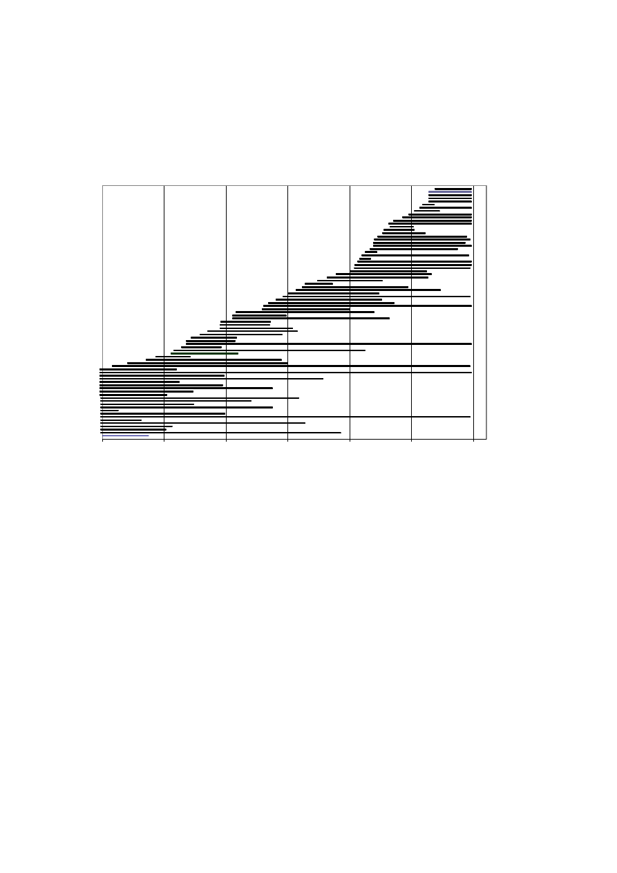
Chart 1

NSW Coal Operators Full data

22097

24497

26897

29297

31697

34097

36497

Date started and finished

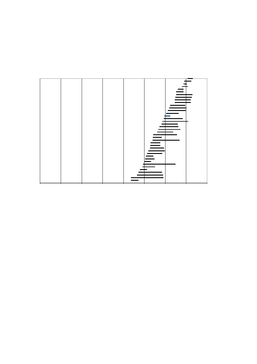
Chart 2

NSW Coal Operators Completed Durations

0

5000

10000

15000

20000

25000

30000

35000

40000

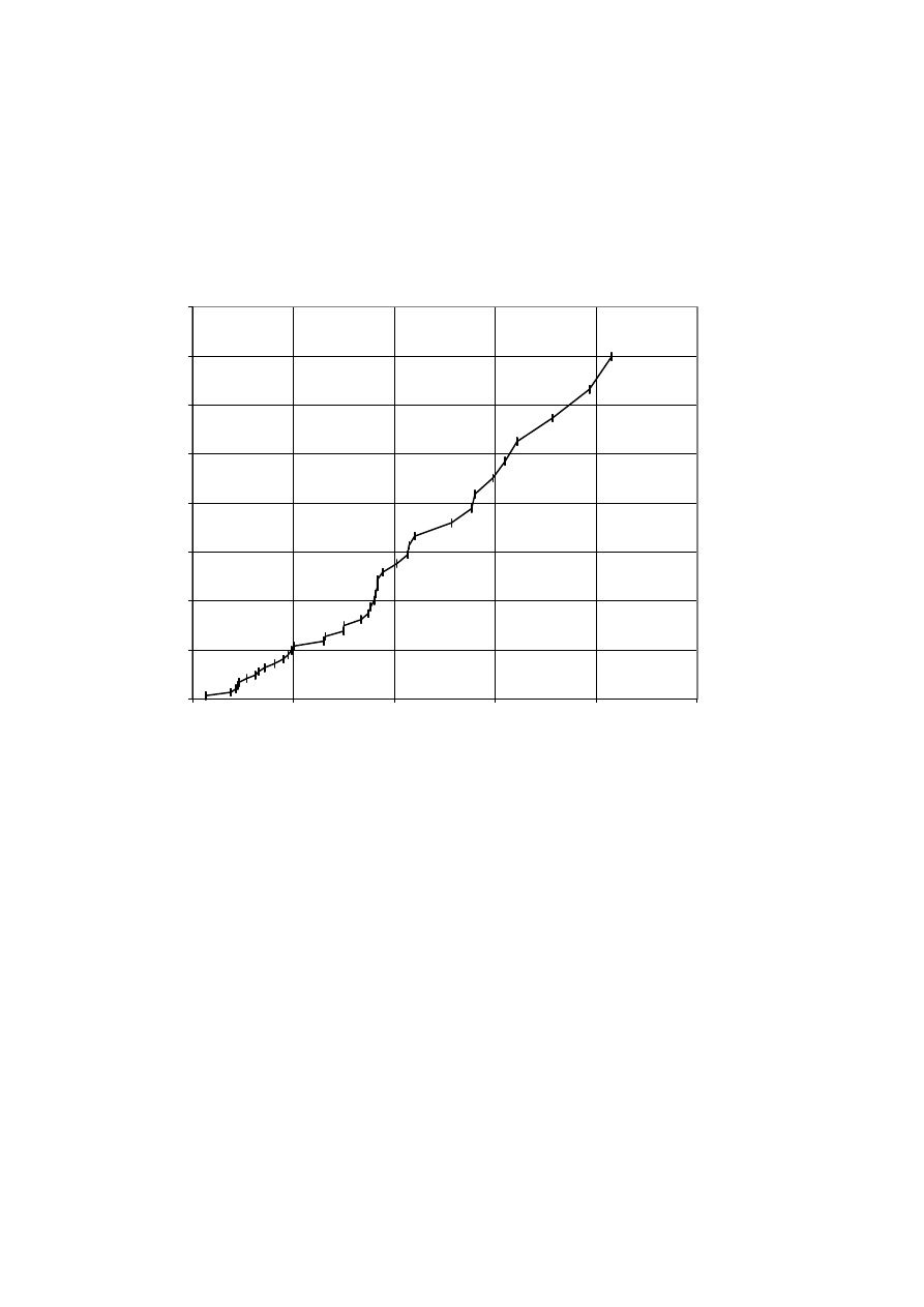
Chart 3

Integrated hazard of Kaplan-Meier product-limit

estimator

0.0

0.2

0.4

0.6

0.8

1.0

1.2

1.4

1.6

0

5

10

15

20

25

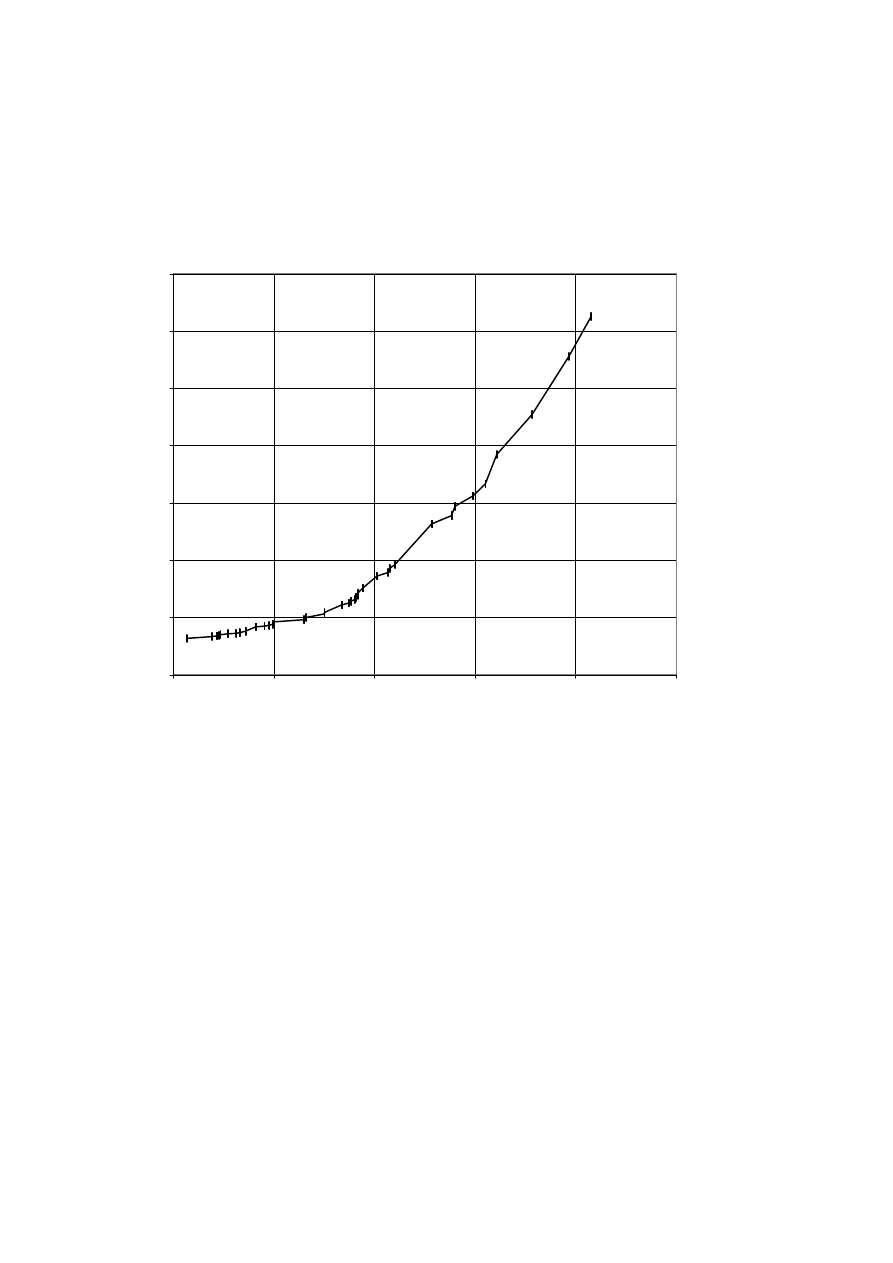
Chart 4

Hazard of the Kaplan-Meier product-limit estimator

0.00

0.02

0.04

0.06

0.08

0.10

0.12

0.14

0

5

10

15

20

25

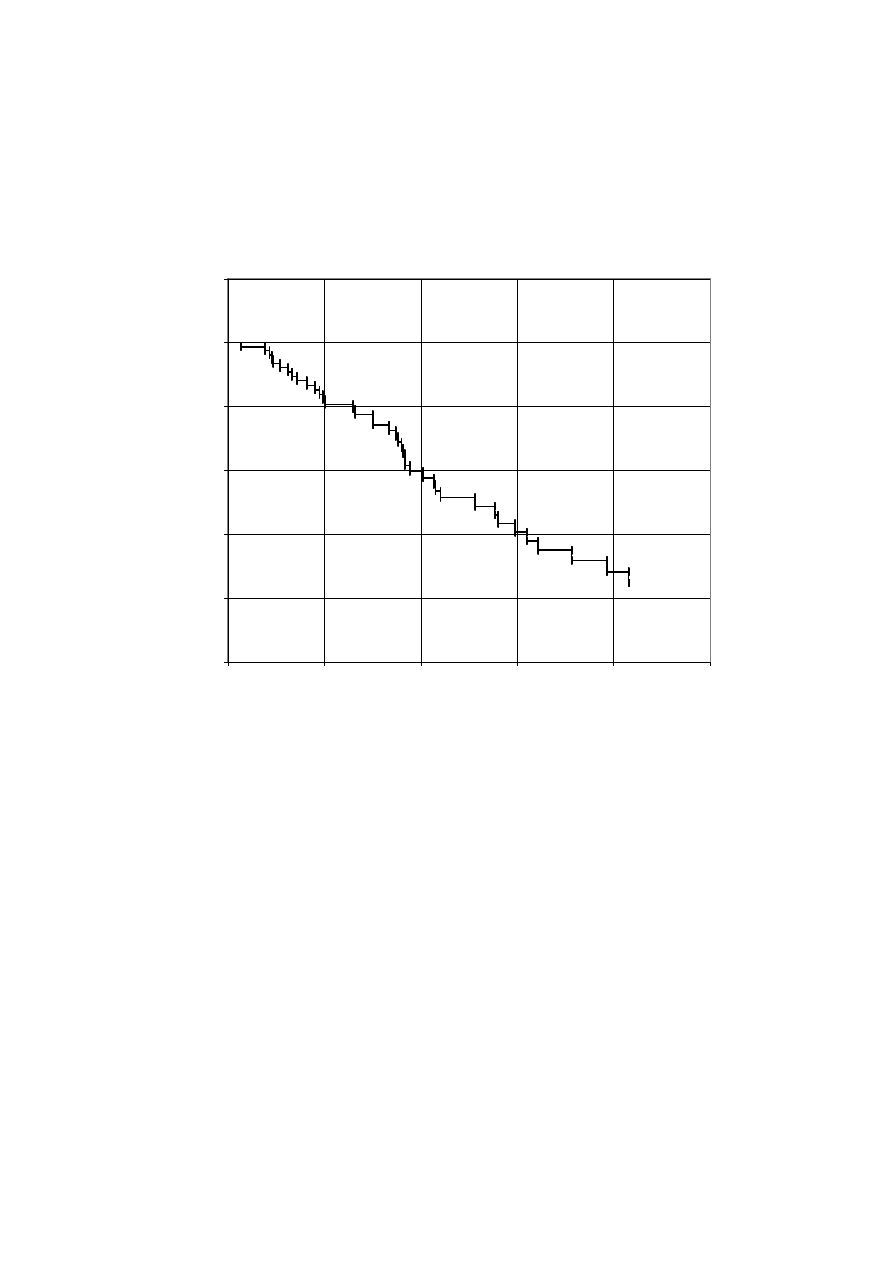
Chart 5

Survivor function of Kaplan-Meier product-limit estimator

0.0

0.2

0.4

0.6

0.8

1.0

1.2

0

5

10

15

20

25

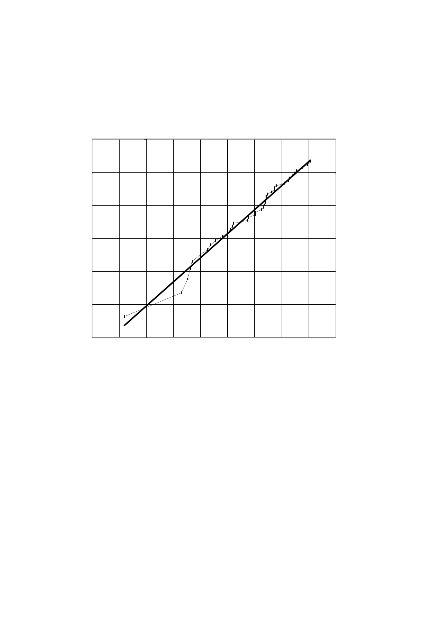
Chart 6a

Weibull plots from Kaplan-Meier product-limit

estimator (uncensored data)

-5

-4

-3

-2

-1

0

1

-1.0

-0.5

0.0

0.5

1.0

1.5

2.0

2.5

3.0

3.5

Linear trend line

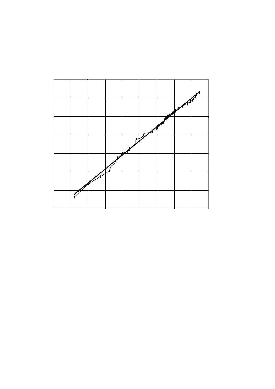
Chart 6b

Weibull plots for full data

-5

-4

-3

-2

-1

0

1

2

-1.0

-0.5

0.0

0.5

1.0

1.5

2.0

2.5

3.0

3.5

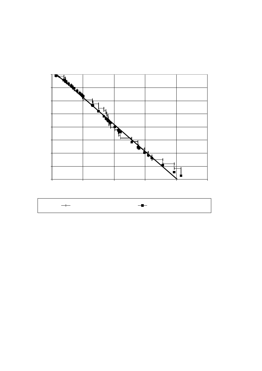
Chart 7a

Survivor functions

0.2

0.3

0.4

0.5

0.6

0.7

0.8

0.9

1

0

5

10

15

20

25

Kaplan-Meier

Weibull from Kaplan-Meier

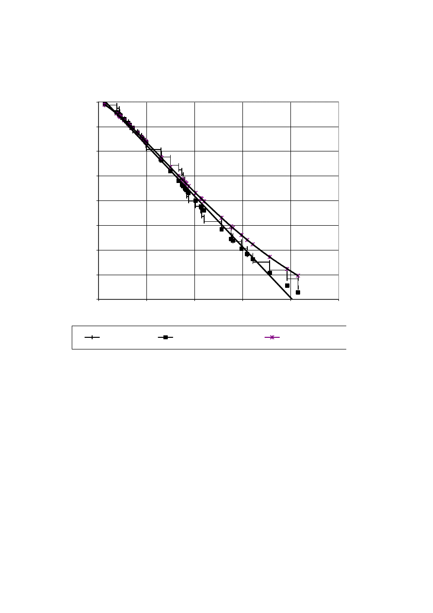
Chart 7b

Survivor functions

0.2

0.3

0.4

0.5

0.6

0.7

0.8

0.9

1

0

5

10

15

20

25

Kaplan-Meier

Weibull from Kaplan-Meier

Weibull from ML estimates

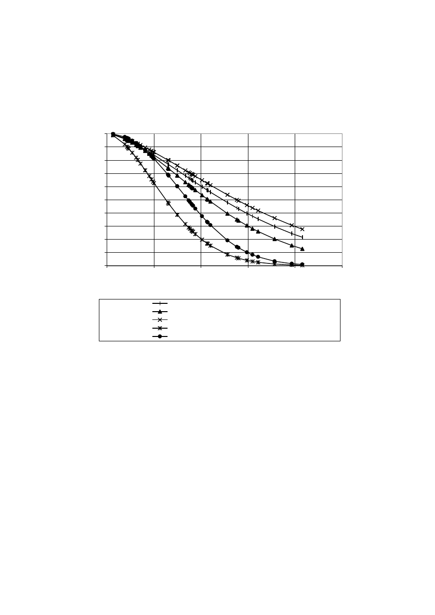
Chart 8

Comparison of all survivor functions

0.0

0.1

0.2

0.3

0.4

0.5

0.6

0.7

0.8

0.9

1.0

0

5

10

15

20

25

Weibull from Kaplan-Meier

Weibull from Medians

Weibull from MLE

Weibull from assuming all durations completed

Weibull using only completed durations

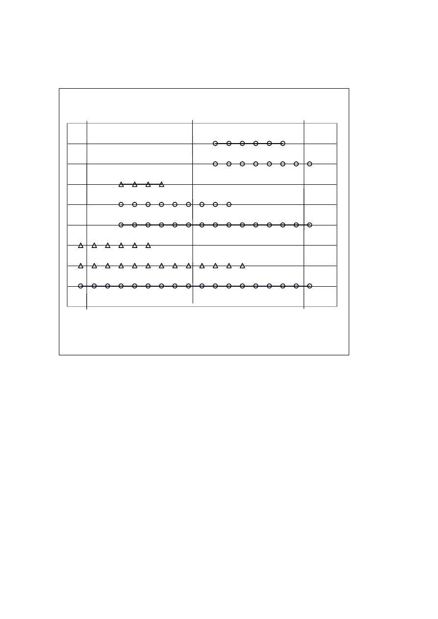
Chart 9

Division into Early and Late sections

Duration length

31/7/60

1/7/79

1/7/99

∆

Early section O Late section

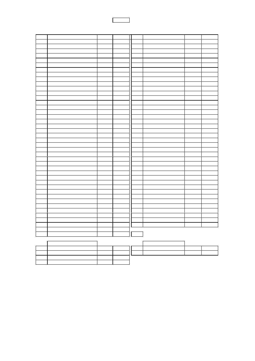
Table 1

NSW Coal Operators 1960 to 1999

Completed durations

Withdrawals

Years

Operator

Start

Finish

Years

Operator

Start

Finish

0.7

Tomen

1/11/94

1/07/95

1.0

Gympie

1/07/98

1/07/99

1.9

Oakdale

1/08/97

1/07/99

1.4

Clinton Nattai Collieries

30/06/60

1/12/61

2.2

Coal & Allied no.2

1/03/91

27/04/93

1.9

Allied Meridian

25/08/97

1/07/99

2.3

AMP

1/12/93

1/03/96

2.6

Austral Coal Ltd

1/12/96

1/07/99

2.3

Consolidation Coal

1/05/82

1/09/84

3.3

Ingwe

1/03/96

1/07/99

2.7

TNT

30/08/90

12/05/93

3.9

Bellambi

30/06/60

1/06/64

3.1

Genders mining Co P L

7/05/66

19/06/69

4.0

Advance

1/07/95

1/07/99

3.3

Wallamaine

16/03/70

3/07/73

4.0

AGIP

1/07/90

1/07/94

3.6

Macdonald Bros P L

1/03/69

1/10/72

4.0

AMCI (Namoi)

1/07/95

1/07/99

4.1

CIM

1/06/95

1/07/99

4.0

Brimstone

1/07/95

1/07/99

4.5

Bulli Main Collieries Pty Ltd

1/10/69

4/04/74

4.9

Placer

29/06/60

1/06/65

4.8

CSR

1/04/73

1/01/78

5.0

Abelshore

1/07/94

1/07/99

4.9

Ampol/TNT (Bulkships)

1/02/73

1/01/78

6.1

Cyprus

12/05/93

1/07/99

5.0

Woonona Mining & Engineering 24/09/74

1/10/79

6.5

Hebburn

30/06/60

1/01/67

6.5

Bond

30/06/83

1/01/90

6.8

Peabody

30/09/92

1/07/99

6.6

Slater Walker

1/01/68

2/08/74

7.3

Barix

30/06/60

6/10/67

7.5

Boral

2/03/87

1/09/94

7.5

Wancol

30/06/60

8/01/68

7.5

Muswellbrook 2

1/01/73

1/07/80

7.8

Cumnock

1/10/91

1/07/99

8.4

Eric Newham (Wallerawang)

1/01/71

11/05/79

7.9

Newcastle Wallsend Coal

30/06/60

1/06/68

8.7

Pacific Copper

6/10/77

18/06/86

8.3

Henry Walker

1/04/91

1/07/99

8.8

Denehurst

1/03/89

1/01/98

9.4

Maintland Mining Co P L

30/06/60

14/11/69

9.0

FAI

1/01/90

1/01/99

9.5

Gifford R A Pty Ltd

30/06/60

31/12/69

9.1

Consolidated Press

1/07/80

31/07/89

9.9

Centennial

2/08/89

1/07/99

9.2

Hartogen

2/11/71

1/01/81

9.9

Idemitsu

31/07/89

1/07/99

9.2

Noette (Coalpac)

1/08/89

1/10/98

11.5 Exxon

1/01/88

1/07/99

9.4

Clutha

13/09/85

14/02/95

11.8 Sumitomo

1/09/87

1/07/99

10.1 AMI

17/09/84

1/11/94

12.0 South Coast Equipment

1/07/87

1/07/99

10.7 BP Australia Holdings Ltd

1/04/79

1/12/89

12.5 Muswellbrook 1

30/06/60

1/01/73

10.7 Coatain

1/01/82

30/09/92

12.6 R W Miller

30/06/60

1/02/73

11.0 Savage

1/04/88

7/04/99

12.8 Buchannan

30/06/60

1/04/73

12.8 Howard Smith

1/05/78

1/03/91

15.7 Gollin

30/06/60

1/03/76

13.8 D K Ludwig

1/06/65

1/04/79

17.8 Mt Sugarloaf Colls P L

30/06/60

1/04/78

14.0 White

1/01/75

1/01/89

19.6 Shell

1/12/79

1/07/99

14.9 Caltex

10/04/81

1/03/96

21.4 Bayswater

30/06/60

4/12/81

15.5 Consolidated Gold Fields

1/06/64

1/12/79

21.6 Hartley Valley Coal Co

11/12/77

1/07/99

16.1 Oakbridge

2/08/74

3/09/90

22.5 Avondale

30/06/60

17/01/83

17.8 Coal & Allied no.1

30/06/60

1/05/78

23.2 North Bulli

30/06/60

16/09/83

19.7 Peko-Wallsend

1/06/68

1/02/88

25.2 Austen & Butta

30/06/60

20/09/85

20.8 Goodsir & Copper P L

30/06/60

10/04/81

29.8 Big Ben Holdings

1/10/69

1/07/99

37.6 CRA

1/12/61

1/07/99

39 count

40 count

Deletions

Deletions

0.2 Pasminco

7/04/99

1/07/99

39.0 BHP

30/06/60

1/07/99

0.5 HIH

1/01/99

1/07/99

39.0 State Govt

30/06/60

1/07/99

0.7 Elders

1/10/88

29/06/89

0.8 North Broken Hill

1/02/88

31/10/88

Table 2

Kaplan-Meier product-limit analysis

Completed

Uncensored

Number

Survivor

Hazard

Integrated

Weibull analysis

Weibull

Weibull

duratons

durations

at

function

dj/nj

hazard

eta = 15.67

distributio

n

survivor

Years

Years

risk

beta = 1.5

function

function

tj

d(t)

Tj

n(t)

S(t)

H(t)

H(t) = -ln[S(t)]

Ln(t)

LnLn(1/S)

F(t)

1 -F(t)

0.67

1

0.67

79

0.987

0.013

0.013

-0.405

-4.363

0.008

0.992

1.92

1

1.00

75

0.974

0.01

0.026

0.651

-3.643

0.040

0.960

2.16

1

1.42

74

0.961

0.01

0.040

0.768

-3.225

0.048

0.952

2.25

1

1.85

73

0.948

0.01

0.054

0.811

-2.927

0.051

0.949

2.33

1

1.92

72

0.935

0.01

0.068

0.847

-2.695

0.054

0.946

2.70

1

2.16

70

0.921

0.01

0.082

0.993

-2.502

0.067

0.933

3.12

1

2.25

69

0.908

0.01

0.097

1.137

-2.338

0.082

0.918

3.30

1

2.33

68

0.895

0.01

0.111

1.193

-2.195

0.089

0.911

3.58

1

2.58

66

0.881

0.02

0.127

1.276

-2.067

0.101

0.899

4.08

1

2.70

60

0.866

0.02

0.143

1.407

-1.942

0.121

0.879

4.51

1

3.12

59

0.852

0.02

0.161

1.506

-1.829

0.140

0.860

4.75

1

3.30

58

0.837

0.02

0.178

1.558

-1.726

0.150

0.850

4.92

1

3.33

57

0.822

0.02

0.196

1.593

-1.632

0.158

0.842

5.02

1

3.58

54

0.807

0.02

0.214

1.613

-1.540

0.162

0.838

6.50

1

3.92

52

0.792

0.02

0.234

1.872

-1.454

0.231

0.769

6.59

1

4.00

50

0.776

0.02

0.254

1.885

-1.371

0.235

0.765

7.497

1

4.00

47

0.759

0.02

0.275

2.015

-1.289

0.278

0.722

7.500

1

4.00

46

0.743

0.02

0.297

2.015

-1.213

0.278

0.722

8.36

1

4.00

41

0.725

0.02

0.322

2.124

-1.133

0.319

0.681

8.70

1

4.08

40

0.707

0.03

0.347

2.163

-1.057

0.335

0.665

8.83

1

4.51

39

0.688

0.03

0.373

2.179

-0.985

0.342

0.658

9.00

1

4.75

38

0.670

0.03

0.400

2.197

-0.916

0.350

0.650

9.08

1

4.92

37

0.652

0.03

0.427

2.206

-0.850

0.354

0.646

9.16

1

4.92

36

0.634

0.03

0.456

2.215

-0.786

0.357

0.643

9.17

1

5.00

35

0.616

0.03

0.485

2.216

-0.724

0.358

0.642

9.42

1

5.02

33

0.597

0.03

0.515

2.243

-0.663

0.369

0.631

10.12

1

6.14

29

0.577

0.03

0.550

2.315

-0.597

0.402

0.598

10.67

1

6.50

28

0.556

0.04

0.587

2.367

-0.533

0.427

0.573

10.75

1

6.50

27

0.535

0.04

0.625

2.375

-0.471

0.431

0.569

11.02

1

6.59

26

0.515

0.04

0.664

2.399

-0.410

0.443

0.557

12.83

1

6.75

19

0.488

0.05

0.718

2.552

-0.331

0.522

0.478

13.83

1

7.27

18

0.461

0.06

0.775

2.627

-0.255

0.563

0.437

14.00

1

7.497

17

0.434

0.06

0.836

2.639

-0.180

0.569

0.431

14.89

1

7.500

16

0.406

0.06

0.900

2.701

-0.105

0.604

0.396

15.50

1

7.52

15

0.379

0.07

0.969

2.741

-0.031

0.626

0.374

16.09

1

7.75

13

0.350

0.08

1.049

2.778

0.048

0.647

0.353

17.84

1

7.92

11

0.318

0.09

1.145

2.881

0.135

0.704

0.296

19.67

1

8.25

9

0.283

0.11

1.262

2.979

0.233

0.757

0.243

20.78

1

8.36

8

0.248

0.13

1.396

3.034

0.334

0.785

0.215

8.70
8.83

Tj (cont.)

9.00

12.83

9.08

13.83

9.16

14.00

9.17

14.89

9.37

15.50

9.42

15.67

9.50

16.09

9.91

17.75

9.92

17.84

10.12

19.58

10.67

19.67

10.75

20.78

11.02

21.43

11.50

21.56

11.83

22.55

12.00

23.21

12.50

25.22

12.59

29.75

12.75

37.58

Count =

79

Table 3

Summary of results

Completed

Likelihood

Log

eta

beta

mean

median

Full data [1]

durations

Withdrawals

likelihood Scale Shape

Weibull from Median values

39

40

1.10E-69

-158.8

9.6

1.61

8.6

7.64

Weibull from MLE parameters

39

40

1.92E-67

-153.6

17.6

1.51

15.8

13.8

Weibull MLE

39

0

5.17E-51

-115.8

10.2

2.19

9.0

8.63

(only completed durations)
Weibull MLE

79

0

9.34E-112

-255.7

7.7

1.77

6.8

6.26

(assume all completed)
Weibull from Kalpan-Meier

39

40

9.71E-68

-154.3

15.7

1.52

14.1

12.31

Early section [2]
MLE 10

19

5.77E-20

-44.299

27.8

1.17

26.4

20.33

Late section [3]
MLE 20

30

1.3132E-36

-82.621

21.4

1.14

20.5

15.55

mean =

median =

[5]

[5]

[4]

Max likelihood beta =
[5]

Max likelihood eta =
[5]

Likelihood function =
[5]

N = number of completed durations
r = number of completed durations
t = completed durations
T = withdrawals

[1] Data from 30/6/60 to 1/7/99, completed durations and withdrawals from left and right censoring
[2] Those started before 1/7/79 and finished by 30/6/79 plus those started before 1/7/60 and finished after 30/6/79
[3] Started after 30/6/60 and not finished by 30/6/79 and all started after 30/6/79
[4] Gamma function from Beyer (1976) "Standard Mathematical Tables" and using formula
[5] Abernethy (1993)

( )

β

η

1

2

ln

0

1

ln

1

ln

1

1

1

=

β

−

−

∑

∑

∑

=

=

β

=

β

r

i

i

N

i

i

i

N

i

i

t

r

t

t

t

β

=

β

























=

η

∑

1

1

ˆ

r

t

N

i

i













β

+

β

Γ

η

1

∏

∏

=













η

−

=









η

−

−

β







































η









η

β

=

β

β

k

j

T

r

i

t

i

j

i

e

e

t

L

1

1

1

(

)

( )

x

x

x

Γ

=

+

Γ

1

Table 4

Period commencing 1st July

1960

1965

1970

1975

1980

1985

1990

Completed durations

39

35

29

21

18

12

6

Early censoring

18

19

18

20

14

13

12

Late censoring

22

22

22

21

21

21

21

Total withdrawals

40

41

40

41

35

34

33

Total

79

76

69

62

53

46

39

MLE beta

1.35

1.23

1.40

1.12

1.03

0.94

0.63

MLE eta

17.9

19.93

21.05

28.80

30.16

40.06

160.3

Table5

Survivor

Completed

Rank

function

durations

i

S

LnLn(1/S)

t

Ln(t)

Ln(t)*Ln(t)

Wi

L1

W(n+i)

L2

1

0.98

-3.68

0.67

-0.41

0.16

0.03

-0.01

-1.07

0.43

2

0.95

-2.97

1.92

0.65

0.42

0.05

0.03

-1.10

-0.72

3

0.93

-2.55

2.16

0.77

0.59

0.08

0.06

-1.12

-0.86

4

0.90

-2.25

2.25

0.81

0.66

0.11

0.09

-1.13

-0.92

5

0.88

-2.01

2.33

0.85

0.72

0.13

0.11

-1.14

-0.96

6

0.85

-1.82

2.70

0.99

0.99

0.16

0.16

-1.13

-1.13

7

0.83

-1.65

3.12

1.14

1.29

0.19

0.22

-1.12

-1.28

8

0.80

-1.50

3.30

1.19

1.42

0.22

0.27

-1.11

-1.33

9

0.78

-1.37

3.58

1.28

1.63

0.25

0.33

-1.09

-1.40

10

0.75

-1.25

4.08

1.41

1.98

0.29

0.40

-1.07

-1.51

11

0.73

-1.13

4.51

1.51

2.27

0.32

0.48

-1.04

-1.57

12

0.70

-1.03

4.75

1.56

2.43

0.36

0.56

-1.01

-1.58

13

0.68

-0.93

4.92

1.59

2.54

0.39

0.63

-0.97

-1.55

14

0.65

-0.84

5.02

1.61

2.60

0.43

0.69

-0.93

-1.50

15

0.63

-0.76

6.50

1.87

3.51

0.47

0.88

-0.88

-1.66

16

0.60

-0.67

6.59

1.88

3.55

0.51

0.96

-0.83

-1.57

17

0.58

-0.59

7.50

2.01

4.06

0.55

1.11

-0.77

-1.56

18

0.55

-0.51

7.50

2.01

4.06

0.60

1.20

-0.71

-1.43

19

0.53

-0.44

8.36

2.12

4.51

0.64

1.37

-0.64

-1.36

20

0.50

-0.37

8.70

2.16

4.68

0.69

1.50

-0.56

-1.21

21

0.48

-0.30

8.83

2.18

4.75

0.74

1.62

-0.48

-1.04

22

0.45

-0.23

9.00

2.20

4.83

0.80

1.75

-0.38

-0.84

23

0.43

-0.16

9.08

2.21

4.87

0.86

1.89

-0.28

-0.61

24

0.40

-0.09

9.16

2.22

4.91

0.92

2.03

-0.16

-0.36

25

0.38

-0.02

9.17

2.22

4.91

0.98

2.17

-0.04

-0.08

26

0.35

0.05

9.42

2.24

5.03

1.05

2.35

0.10

0.23

27

0.33

0.12

10.12

2.31

5.36

1.12

2.60

0.26

0.59

28

0.30

0.19

10.67

2.37

5.60

1.20

2.85

0.43

1.01

29

0.28

0.26

10.75

2.37

5.64

1.29

3.07

0.62

1.47

30

0.25

0.33

11.02

2.40

5.76

1.39

3.33

0.84

2.01

31

0.23

0.40

12.83

2.55

6.51

1.49

3.81

1.09

2.78

32

0.20

0.48

13.83

2.63

6.90

1.61

4.23

1.38

3.61

33

0.18

0.56

14.00

2.64

6.96

1.74

4.60

1.71

4.52

34

0.15

0.64

14.89

2.70

7.29

1.90

5.12

2.11

5.70

35

0.13

0.73

15.50

2.74

7.51

2.08

5.70

2.60

7.13

36

0.10

0.83

16.09

2.78

7.72

2.30

6.40

3.22

8.95

37

0.08

0.95

17.84

2.88

8.30

2.59

7.46

4.06

11.69

38

0.05

1.10

19.67

2.98

8.87

3.00

8.92

5.28

15.74

39

0.03

1.31

20.78

3.03

9.20

5.45

16.55

13.58

41.21

NB The survivor function S is calculated using (n + 1) because the data must be assumed to be from
a Weibull population which is infinite.

0.5899

0.0823

Using Shapiro table 6.4 p.6.17, sample size 39 and limits 0.05 and .95
the lower and upper values are:

lower

upper

0.4403051

0.862093

As Wp lies between these two extreme value
there is no reason to reject the null hypothesis of a Weibull
distribution

W = nb

2

/S

2

b = (0.6079L

2

– 0.2570L

1

)/n

Table 6

Johnson method of median ranks

Benard

Benard

(n+1) = 73

Adjusted

median

median

mean

Adjusted

rank

rank

Durations

Increment

rank

mean rank (proportion) Survivor function

0.7

0

1

1

0.01

0.99

1.0

2.04

0.02

0.98

1.4

3.09

0.04

0.96

1.9

4.13

0.05

0.95

1.9

1.04

2.04

5.17

0.07

0.93

2.2

1.04

3.09

6.23

0.08

0.92

2.3

1.04

4.13

7.29

0.10

0.90

2.3

1.04

5.17

8.35

0.11

0.89

2.6

9.43

0.13

0.87

2.7

1.06

6.23

10.61

0.14

0.86

3.1

1.06

7.29

11.79

0.16

0.84

3.3

1.06

8.35

12.96

0.17

0.83

3.3

14.14

0.19

0.81

3.6

1.08

9.43

15.37

0.21

0.79

3.9

16.62

0.23

0.77

4.0

17.90

0.24

0.76

4.0

19.24

0.26

0.74

4.0

20.59

0.28

0.72

4.0

22.09

0.30

0.70

4.1

1.18

10.61

23.58

0.32

0.68

4.5

1.18

11.79

25.08

0.34

0.66

4.8

1.18

12.96

26.58

0.36

0.64

4.9

1.18

14.14

28.08

0.38

0.62

4.9

29.57

0.40

0.60

5.0

31.07

0.43

0.57

5.0

1.23

15.37

32.62

0.45

0.55

6.1

34.38

0.47

0.53

6.5

1.25

16.62

36.13

0.49

0.51

6.5

37.89

0.52

0.48

6.6

1.28

17.90

39.65

0.54

0.46

6.8

42.21

0.58

0.42

7.3

44.78

0.61

0.39

7.5

1.34

19.24

47.34

0.65

0.35

7.5

1.34

20.59

49.91

0.69

0.31

7.5

52.47

0.72

0.28

7.8

55.41

0.76

0.24

7.9

58.93

0.81

0.19

8.3

63.62

0.87

0.13

8.4

1.50

22.09

68.31

0.94

0.06

8.7

1.50

23.58

count = 39

8.8

1.50

25.08

9.0

1.50

26.58

9.1

1.50

28.08

9.2

1.50

29.57

9.2

1.50

31.07

mean

9.4

Durations

Increment

rank

9.4

1.55

32.62

continued

continued continued

9.5

15.7

9.9

16.1

2.93

55.41

9.9

17.8

10.1

1.76

34.38

17.8

3.52

58.93

10.7

1.76

36.13

19.6

10.7

1.76

37.89

19.7

4.69

63.62

11.0

1.76

39.65

20.8

4.69

68.31

11.5

Exclude

21.4

11.8

Exclude

21.6

12.0

Exclude

22.5

12.5

Exclude

23.2

12.6

Exclude

25.2

12.8

Exclude

29.8

12.8

2.57

42.21

Exclude

37.6

13.8

2.57

44.78

Count = 79

14.0

2.57

47.34

14.9

2.57

49.91

15.5

2.57

52.47

[1] Bold and italicised data are withdrawals