
Field Manual
No. 5-33
*FM 5-33
HEADQUARTERS
DEPARTMENT OF THE ARMY
Washington, DC, 11 July 1990
Terrain Analysis
Preface
SCOPE
Terrain analysis, an integral part of the intelligence preparation of the battlefield
(IPB), plays a key role in any military operation. During peacetime, terrain analysts
build extensive data bases for each potential area of operations. They provide a base for
all intelligence operations, tactical decisions, and tactical operations. They also sup-
port the planning and execution of most other battlefield functions. Because terrain
features continually undergo change on the earth’s surface, data bases must be
continuously revised and updated.
PURPOSE
This field manual prescribes basic doctrine and is intended to serve as a primary
source of the most current available information on terrain analysis procedures for all
personnel who plan, supervise, and conduct terrain analysis. The manual discusses the
impact of the terrain and the weather on operations.
USER INFORMATION
The proponent of this publication is the US Army Engineer School. Submit changes for
improving the publication on DA Form 2028 (Recommended Changes to Publications
and Blank Forms) to Commandant, Directorate of Training and Doctrine, US Army En-
gineer School, ATTN: ATSE-TDM-P, Ft. Leonard Wood, MO 65473-6500.
Approved for public release; distribution is unlimited.
Unless otherwise stated, whenever the masculine gender is used, both men and
women are included.
*This publication supersedes FM 21-33, 15 May 1978, and FM 30-10, 27 March 1972.
i
FM 5-33
C1
HEADQUARTERS
CHANGE
DEPARTMENTS OF THE ARMY
NO. 1
Washington, DC, 8 September 1992
Terrain Analysis
1. Change FM 5-33, 11 July 1990, as follows:
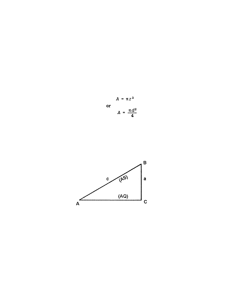
Page 10-1. Table 10-1, 2. Circles, change formulas to read:
Page 10-3. Table 10-3. Change entry in last line, last column, to ’’118 lb.”
Page 10-4. To the second paragraph under the subheading “Six Functions’’add the following
drawing:
2. Post these changes according to DA Pamphlet 310-13.
3. File this transmittal sheet in front of the publication.
DISTRIBUTION RESTRICTION. Approved for public release; distribution is unlimited.

By Order of the Secretary of the Army:
Official:
GORDON R. SULLIVAN
General, United States Army
Chief of Staff
MILTON H. HAMILTON
Administrative Assistant to the
Secretary of the Army
02181
DISTRIBUTION:
Active Army, USAR, and ARNG:
To be distributed in accordance
with DA Form 12-11E, requirements for FM 5-33, Terrain Analysis
(Qty rqr block no. 4329).

PART ONE
Terrain Evaluation and Verification
FM 5-33
Natural Terrain
Chapter 1
SURFACE CONFIGURATION
Maneuver commanders must have accurate intelligence on the surface configura-
tion of the terrain. Ravines, embankments, ditches, plowed fields, boulder fields,
and rice-field dikes are typical surface configurations that influence military
activities. Elevations, depressions, slope, landform type, and surface roughness
are some of the terrain factors that affect movement of troops, equipment, and
material.
Landforms
Landforms are the physical expression of the land surface. The principal groups
of landforms are plains or plateaus, hills, and mountains. Within each of these
groups are surface features of a smaller size, such as flat lowlands and valleys.
Each type results from the interaction of earth processes in a region with given
climate and rock conditions. A complete study of a landform includes determina-
tion of its size, shape, arrangement, surface configuration, and relationship to the
surrounding area.
Relief
Local relief is the difference in elevation between the points in a given area. The
elevations or irregularities of a land surface are represented on graphics by
contours, hypsometric tints, shading, spot elevations, and hachures.
Slope or Gradient
Slope can be expressed as the slope ratio or gradient, the angle of slope, or the
percent of slope. The slope ratio is a fraction in which the vertical distance is the
numerator and the horizontal distance is the denominator. The angle of slope in
degrees is the angular difference the inclined surface makes with the horizontal
plane. The tangent of the slope angle is determinedly dividing the vertical distance
by the horizontal distance between the highest and lowest elevations of the inclined
1-1

FM 5-33
Terrain Evaluation and Verification
PART ONE
surface. The actual angle is found by using trigonometric tables. The percent of
slope is the number of meters of elevation per 100 meters of horizontal distance.
Slope information that is available to the analyst in degrees or in ratio values may
be converted to percent of slope by using a nomogram.
VEGETATION FEATURES
Plant cover can affect military tactics, decisions, and operations. Perhaps the
most important is concealment. To make reliable evaluations when preparing
vegetation overlays, analysts must collect data on the potential effects of vegetation
on vehicular and foot movement, rover and concealment, observation, airdrops,
and construction materials.
Types
The types of vegetation in an area can give an indication of the climatic conditions,
soil, drainage, and water supply. Terrain analysts are interested in trees, scrubs and
shrubs, grasses, and crops.
On military maps, any perennial vegetation high enough to conceal troops or thick
enough to be a serious obstacle to free passage is classified as woods or brushwood.
Although trees provide good cover and concealment, they can present problems to
movement of armor and wheeled vehicles. Woods also slow down the movement
of dismounted troops. Individual huge trees are seldom so close together that a
tank cannot move between them, but the space between them is often filled by
smaller trees or brush. Closely spaced trees are usually fairly small and can be
pushed over by a tank; however, the resulting pileup of vegetation may stop the
tank. Trees that can stop a wheeled vehicle are usually too closely spaced to bypass.
The pileup effect from pushing over vegetation is greater for wheeled vehicles than
for tanks.
Trees are classified as either deciduous (broadleaf) or coniferous (evergreen).
With the exception of species growing in tropical areas and a few species existing
intemperate climates, most broadleaf trees lose their leaves in the fall and become
dormant until the early spring. Needleleaf trees do not normally lose their leaves
and exhibit only small seasonal changes.
Woodlands or forests are classified according to the dominant local tree type. A
forest is classified as either deciduous or coniferous if it contains at least 60 percent
of that species. Wooded areas that contain less than a 60 percent mixture of either
species are classified as a mixed forest.
Scrubs include a variety of trees that have had their growth stunted because of
soil or climatic conditions. Shrubs comprise the undergrowth in open forests, but
in arid and semiarid areas they are the dominant vegetation. Shrubs normally offer
no serious obstacle to movement and provide good concealment from ground
observation however, they may restrict fields of fire.
For terrain intelligence purposes, grass more than 1 meter high is considered tall.
Grass often improves the trafficability of soils. Very tall grass may provide
concealment for foot troops. Foot movement in savannah grasslands is slow and
tiring; vehicular movement is easy; and observation from the air is easy.
1-2

PART ONE
Terrain Evaluation and Verification
FM 5-33
Field crops constitute the predominant class of cultivated vegetation. Vine crops
and orchards are common but not widespread, and tree plantations are found in
relatively few areas. The size of cultivated areas ranges from paddies covering a
quarter of an acre to vast wheat fields extending for thousands of acres.
In a densely populated agricultural area where all arable land is used for the crop
producing the highest yield, it may be possible to predict the nature of the soils
from information about the predominant crop. Rice, for example, requires fine-
textured soils, while other crops generally must have firm, well-drained land. An
area of orchards or plantations usually consists of rows of evenly spaced trees,
showing evidence of planned planting. This can be distinguished on an aerial
photograph. Usually such an area is free of underbrush and vines. Rice fields are
flooded areas surrounded by low dikes or walls.
Some crops, such as grain, improve the trafficability of soils, while others, such
as vineyards, present a tangled maze of poles and wires and create definite obstacles
to vehicles and dismounted troops. Wheeled vehicles and some tracked vehicles
are unable to cross flooded paddy fields, although they can negotiate them when
the fields are drained and dry or frozen. Sown crops, such as wheat, barley, oats,
and rye, will have a different impact on movement and concealment than those
crops planted in furrows, because they are on a flat surface.
Photographic Texture
Texture is influenced by several variables, including crown shapes, tree spacing,
and tree height. Texture interpretation as a means of identifying forest type requires
knowledge of the texture often associated with each forest type. This knowledge
is acquired through hands-on experience or the use of vegetation keys. With
hands-on experience working with aerial imagery over along period of time and
through the process of trial and error, an analyst can develop a mental catalog to
relate texture in a given geographic area to a specific forest type.
Vegetation keys have been developed through the same trial and error process
but have been documented and are available in the literature. They can be very
useful in certain instances (see Chapter 3 for examples). However, one must
remember that background knowledge of the area of interest is essential and most
keys are specific to tree species, geographic area, time of year, film type, and
photoscale. When using color or color infrared film, tone is often referred to as
hue and is represented as shades of the color image.
Photographic Tone
Tone is also very important and is often applied to the problem of forest type
identification. Tone is influenced primarily by stand density, reflectivity, and
location of the tree stand with respect to the photographic center. When using
panchromatic and black and white infrared film, photographic tone is represented
by shades of gray. For example, in most regions of the world, needle leaf trees will
appear darker in tone than broadleaf trees on panchromatic film given equivalent
stand density. This tone difference is due to higher reflectivity of broadleaf trees
in the region of the electromagnetic spectrum to which the film is sensitive.
1-3

FM 5-33
Terrain Evaluation and Verification
PART ONE
SOIL FEATURES
Since soils vary in their ability to bear weight, their ability to withstand vehicle
passes, and their ease of digging, military planners rely heavily on soil analyses.
Soil type, drainage characteristics, and moisture content affect road construction,
material location, and trafficability determination. The soil factor overlay breaks
down the most probable soil types, characteristics, and distribution.
Describing and classifying soil normally requires exhaustive field sampling and
the expertise of soil scientists. Terrain analysts, however, can produce acceptable
soil factor overlays by examining maps, other factor overlays, aerial photographs,
lab analyses, boring logs, and literature. The reliability of the resulting soil factor
overlays will vary with the reliability of the sources used and the analyst’s ability
to correlate and combine the information correctly.
Determining whether a particular soil will support vehicle passage or the con-
struction of roads and airfields is just a part of the terrain analyst’s job. Since
analysts also provide information on construction materials associated with roads
and airfields, they need a variety of evaluation methods and a good working
knowledge of the physical properties of soil.
Type Determination
For field identification and classification, soils may be grouped into five principal
types: gravel, sand, silt, clay, and organic matter. These types seldom exist
separately but are found in mixtures of various proportions, each contributing its
characteristics to the mixture. Some soils may gain strength under traffic while
others lose it.
Gravel is angular to rounded, bulky rock particles ranging in size from about 0.6
to 7.6 cm (¼ to 3 inches) in diameter. It is classified as coarse or fine; well or
poorly graded; and angular, flat, or rounded. Next to solid bedrock, well-graded
and compacted gravel is the most stable natural foundation material. Weather has
little or no effect on its trafficability. It offers excellent traction for tracked
vehicles; however, if not mixed with other soil, the loose particles may roll under
pressure, hampering the movement of wheeled vehicles.
Sand consists of rock grains from shut 0.6 cm (¼ inch) and smaller. It is
classified as coarse, medium, or fine, and is angular or rounded. Well-graded
angular sand is desirable for concrete aggregate and for foundation material. It is
easy to drain and ordinarily not affected by frost action or moisture. Analysts must
be careful, however, to distinguish between a fine sand and silt. When wet enough
to become compacted or when mixed with clay, sand provides excellent traf-
fixability. Very dry, loose sand is art obstacle to vehicles, particularly on slopes.
Under wet conditions, remoldable sands react to traffic as to fine-gained soils.
They feel somewhat plastic rather than gritty when rolled between the fingers.
Silt consists of natural reek grains. It lacks plasticity and possesses little or no
cohesion when dry. Because of silt’s instability, water will cause it to become soft
or to change to a “quick” condition. When dry, silt provides excellent trafficability,
although it is very dusty. However, it absorbs water quickly and turns to a deep,
soft mud (a quick condition), which is a definite obstacle to movement. When
1-4

PART ONE
Terrain Evaluation and Verification
FM 5-33
ground water or seepage is present, silt exposed to frost action is subject to ice
accumulation and consequent heaving.
Clay generally consists of microscopic particles. Its plasticity and adhesiveness
are outstanding characterisitcs. Depending on mineral composition and proportion
of coarser grains, clays vary from lean (low plasticity) to fat (high plasticity). Many
clays which are brittle or stiff in their undisturbed state become soft and plastic
when worked. When thoroughly dry, clay provides a hard surface with excellent
trafficability; however, it is seldom dry except in arid climates. It absorbs water
very slowly but takes a long time to dry and is very sticky and slippery. Slopes
with a clay surface are difficult or impassable, and deep ruts form rapidly on level
ground. A combination of silt and clay makes a particularly poor surface when
wet.
Chemically deposited and organic sediments are classified on the basis of mode
and source of sedimentations. The identification of highly organic soil is relatively
easy; it contains partially decayed grass, twigs, leaves, and so forth, and has a
characteristic dark brown to black color, a spongy fed, and fibrous texture.
Classification
The terrain analyst uses the field classification technique to determine if the soil
is fine or coarse or if it is remoldable sand. Usually the first two steps will determine
the grain. If it is squeezed and rolled between the fingertips, fine-grained plastic
soil will feel soft and smooth and should produce a ribbon or thread. Remoldable
sands will feel coarser and more abrasive than a fine-grained material.
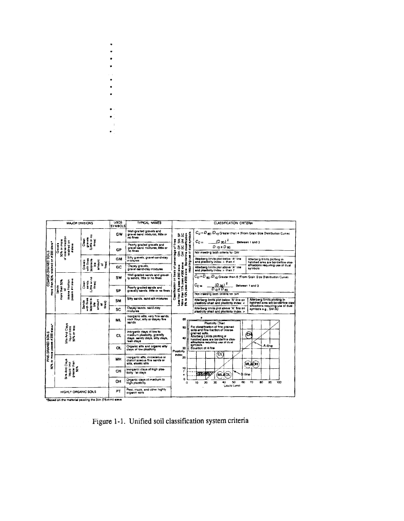
Unified Soil Classification System (USCS)
The Unified Soil Classification System uses a system of two-letter abbreviations
to describe the soil. The primary letter identifies the predominant soil fraction.
The secondary letter further describes the characteristics of the predominant soil
fraction. The percent of gravel, sand, and frees provides the information necessary
to choose the primary letter. See Figure 1-1.
Physical Tests
Before analysts classify soil, they must make four physical tests: gradation, liquid
limit, plastic limit, and odor test.
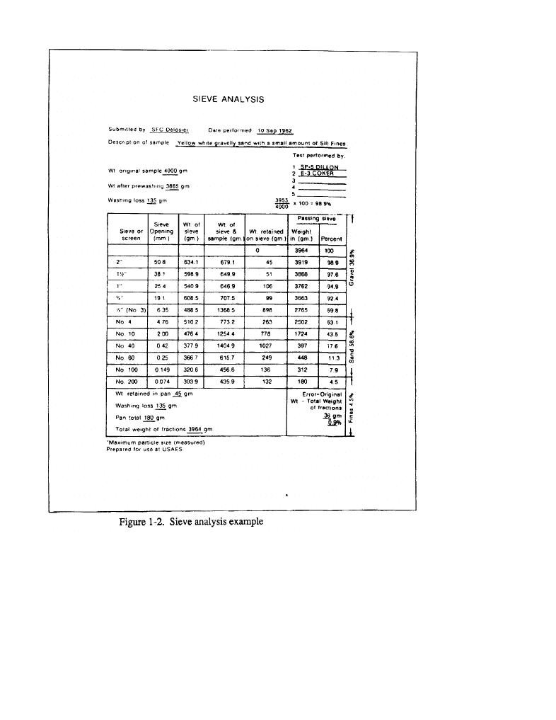
Gradation, or grain-size distribution of a soil, is determined by a sieve analysis.
A sieve analysis is the separation of soil into its fractions. It is made to determine
gradation of material retained on a No. 200 sieve. It indicates whether a soil is well
or poorly graded, and it will show the percentage of fines present. The sieve
analysis may be performed directly on soils that may be readily separated from the
coarser particles.
Sieves that military engineers commonly use have square openings and are
designated as 2-, 1½-, 1-, ¾-, and ¼- inch sieves. They also use the US standard
numbers 4, 10, 20, 40, 60, 100, and 200 sieves. See Figure 1-2 for an example of
a sieve analysis.
PRIMARY LETTERS
G--Gravel
1-5
FM 5-33
Terrain Evaluation and Verification
PART ONE
S--Sand
C--Clay (Used only with fine-grained soil with 50% tines or greater)
M--Silt
O--Organic
SECONDARY LETTERS
W--Well graded (Used to describe sands containing less than 12% fines)
P--Poor graded
M--Silty Fines (Used with sands and gravels containing less than 5% but
more than or equal to 50% frees)
C--Clay-based Pines
L--Low Compressibility (Used to describe fine-grained soils (silts, clays,
organics)
H--High Compressibility
As soil becomes more moist, it transforms from a plastic to a liquid state. The
liquid limit is the moisture content at which a soil will just begin to flow when
jarred slightly. In conjunction with the plastic limit, it is valuable in proper
identification and classification of fine-grained soils. The liquid limit is usually
expressed as a whole number and is obtained by performing the Atterberg liquid
limit test, which is outlined in TM 5-530.
The plastic limit is the moisture content at which cohesive soil passes from a
semisolid to a plastic state. A soil or soil fraction is called plastic if, at some water
1-6
PART ONE
Terrain Evaluation and Verification
FM 5-33
content, it can be rolled out into thin threads. The moisture content ranges between
a soil sample’s liquid and plastic limits. The larger the plasticity index, the more
plastic the soil (PI = LL - PL). The percent of moisture content, by weight, at which
a 1/8-inch diameter thread begins to crumble is expressed as a whole number when
Note: Gravels will be
retained at
¼
- to 2-inch
sieves, sands at Numbers 4-
100; all fines will be retained
at the No. 200 sieve, allowing
estimation of percentages of
soil categories.
recorded
1-7

FM 5-33
Terrain Evaluation and Verification
PART ONE
Since practically all fine-grained soils contain some clay, most of them will
exhibit some amount of plasticity. Soil plasticity is determined by measuring the
different states a plastic soil undergoes with changing moisture content. When a
fine-grained soil or remoldable sand sample is rolled between two flat surfaces or
between one’s thumb and forefinger, it forms a thread. Highly plastic and nonplas-
tic soils break into short lengths or cannot be formed into ribbons. In the field,
analysts can examine the shape and mineral compositions of coarse-grained soil
by spreading a dry sample on a flat surface, separating the gravel and frees as much
as possible, and estimating the percentages of each. TM 5-530 gives further
information.
Organic soils of the OL and OH groups usually have a distinct odor, which can
be used to aid in identification. This color is especially apparent in fresh samples.
It is gradually reduced when exposed to air, but can be brought out again by heating
a wet sample.
Field Identification
Normally, laboratory equipment will not be available in the field, but analysts can
estimate and tentatively classify without tests. Classifications made under stricter
conditions will be more accurate. We classify soils by particle size distribution.
Where these soil types occur and the amount of area they cover often determine
the suitability of an area for military operations. In general, we prefer coarse-
grained soils for construction and cross-country movements.
Well-graded and poorly-graded soils can usually be distinguished by comparing
the sizes. Poorly-graded soils, however, are more difficult to classify because they
lack one size particle. Principal aids to soil identification and classification are the
shaking test, the dry strength or breaking test, and gully analysis.
Analysts performing the shaking test will alternately shake a wet portion of soil
in the palm of the hand and squeeze between the fingers. Atypical inorganic silt
will become livery, show free water to disappear from siIt soil, and cause the sample
to stiffen and crumble under increasing finger pressure. If the water content is just
right, shaking the broken pieces will cause them to liquefy and flow together. The
portion will change its consistency and the water on the surface will appear or
disappear at a rapid, sluggish, slow, or no-reaction speed. A rapid reaction to this
test is typical for a nonplastic, uniform fine sand, inorganic silt, or diatomaceous
(algae-based) earths. A sluggish reaction indicates slightly plastic inorganic and
organic silts, or very silty clays. An extremely slow or no reaction to the shaking
test is typical for all clays that plot above the A-line on the plasticity chart as well
as for highly plastic organic clays.
The dry strength test readily distinguishes between plastic clays and nonplastic
silts or fine sands. Analysts perform the dry strength or breaking test only on a
smaIl portion of soil, about ½-inch thick and 1½ inches in diameter, that passes
the Number 40 sieve. They prepare this by molding a portion of wet plastic soil
into the size and shape desired and allowing it to air (NOT oven) dry. After the
sample is thoroughly dry, they will attempt to break the soil using their thumbs and
forefingers. If it breaks, they will try to powder it by rubbing the particles together.
Typical reactions obtained in this test for various types of soil are--
1-8

PART ONE
Terrain Evaluation and Verification
FM 5-33
Very highly plastic soil, or very high dry strength. Samples cannot be
broken or powdered by finger pressure.
Highly plastic soil, or high dry strength. Samples will break with great
effort, but they cannot be powdered.
Medium plastic soil, or medium dry strength. Samples will break and
powder with some effort.
Slightly plastic soil, or low dry strength. Samples will break and powder
easily.
Nonplastic soil, or very little or no dry strength. Samples crumble and
powder on being picked up.
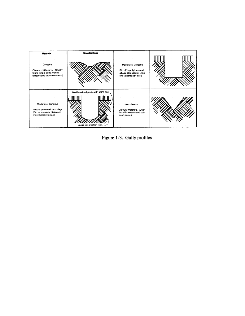
Gullies, sometimes called head water channels, result from erosion caused by
water runoff. They develop in places where water cannot easily filter into the
ground; therefore, it collects and flows in rivulets across the land surface. Gully
analysis can be of great assistance in determining soil types, since these rivulets
often take the shape peculiar to the material over which they flow. Since fine-
grained silts and clays are relatively impervious soils, many gullies develop on their
surfaces. Sands and gravels are rather permeable, and few or no gullies form.
Other factors that govern the extent of gully formation in an area are climate,
vegetation, ground slope, end gradient of individual gullies. Gradient is more
important than intensity, or number, of gullies in revealing soil conditions. The
types of gullies that may be formed in various soil types are--
Gullies in clay. They have a long, uniform, gentle gradient and are
smoothly rounded. Clay soils are impervious and cohesive and often have
a well-developed gully system.
Gullies in silt (primarily loess). They take the form of a U and have steep
sides and generally flat bottoms. The gradient is steep at the head of the
gully but becomes more gentle a short distance away.
Gullies in sand-clay. They are similar to gullies in silts but are more
U-shaped, with a rounded rather than flat bottom. The gradient is nearly
vertical at the head of the gully but levels off rapidly to a very gentle
slope.
Gullies in gravel, sand, or well-graded mixtures with some clays. They
are usually well-defined, short, straight notches (ditches). The cross sec-
tion is a sharp V with a uniform gradient. The steeper gradients are as-
sociated with the coarser materials. See Figure 1-3.
WATER FEATURES
Safe water, in sufficient amounts, is strategically and tactically important to Army
operations. Water that is not properly treated can spread diseases. The control of
and access to water is critical for drinking, sanitation, construction, vehicle opera-
tion, and other military operations. Military planners are concerned with areas with
the highest possibilities for locating usable ground water. They must consider all
feasible sources and methods for developing sources when making plans for water
supply. Quantity and quality are important considerations. Terrain analysts can
use the methods and systems available to locate both surface and subsurface water
resources.
1-9
FM 5-33
Terrain Evaluation and Verification
PART ONE
Quantity
Water quantity depends on the climate of the area. Plains, hills, and vegetation
are good indicators of water sources.
Large springs are the best sources of water in karstic plains and plateaus. Wells
may produce large amounts if they tap underground streams. Shallow wells in
low-lying lava plains normally produce large quantities of ground water. In lava
uplands, water is more difficult to find, wells are harder to develop, and careful
prospecting is necessary to obtain adequate supplies. In wells near the seacoast,
excessive withdrawal of freshwater may lower the water table, allowing infiltration
of saltwater that ruins the well and the surrounding aquifer.
Springs and wells near the base of volcanic cones may yield fair quantities of
water, but elsewhere in volcanic cones the ground water is too far below the surface
for drilling to be practicable. Plains and plateaus in arid climates generally yield
small, highly mineralized quantities of ground water. In semiarid climates, follow-
ing a severe drought, an apparently dry streambed frequently may yield consider-
able amounts of excellent subsurface water. Ground water is abundant in the plains
of humid tropical regions, but it is usually polluted. In arctic and subarctic plains,
wells and springs fed by ground water above the permafrost are dependable only
in summer; some of the sources freeze in winter, and subterranean channels and
outlets may shift in location. Wells that penetrate aquifers within or below the
permafrost are good sources of perennial supply.
Adequate supplies of ground water are hard to obtain in hills and mountains
composed of gneiss, granite, and granite-like rocks. They may contain springs and
shallow wells that will yield water in small amounts.
1-10

PART ONE
Terrain Evaluation and Verification
FM 5-33
Tree species can also indicate local ground water table presence. Deciduous trees
tend to have far-reaching root systems indicating a water table close to the ground
surface. Coniferous trees tend to have deep root systems, which depict the ground
water table as being farther away from the ground surface. In desert environments,
vegetation is scant and specialized to withstand the stress of desert life. Vegetation
type is dependent on the water table of that location. Palm trees indicate water
within 2 or 3 feet, salt grass indicates water within 6 feet, and cottonwood and
willow bees indicate water within 10 to 12 feet. The common sage, greasewood,
and cactus do not indicate water levels.
Quality
Quality will vary according to the source and the season, the kind and amount of
bacteria, and the presence of dissolved matter or sediment. Color, turbidity, odor,
taste, mineral content, and contamination determine the quality of water. Brackish
water is found in many regions throughout the world but most frequently along sea
coasts or as ground water in arid or semiarid climates.
Contamination
Potable water is free from disease-causing organisms and excessive amounts of
mineral and organic matter, toxic chemicals, and radioactivity. Although surface
water is ordinarily more contaminated than other sources, it is commonly selected
for use in the field because it is more accessible in the quantity required. Ground
water is usually less contaminated than surface water and is, therefore, a more
desirable water source. However, the use of ground water by combat units is
usually limited unless existing wells are available. Rain, melted snow, or melted
ice may be used in special instances where neither surface nor ground water is
available. Water from these sources must be disinfected before drinking.
Pollution
Water may be contaminated but not polluted. Streams in inhabited regions are
commonly polluted, with the sediment greatest during flood stages. Streams fed
by lakes and springs with a uniform flow are usually clear and vary less in quality
than do those fed mainly by surface runoff. Generally, the quality of water in large
lakes is excellent, with the purity increasing with the distance from the shore. Very
shallow lakes and small ponds are usually polluted.
Porosity and Permeability
The water-bearing capability of a natural material is determined by porosity and
permeability. The amount of porosity depends on the number of open spaces in
the material. The permeability of rock is its capacity for transmitting a fluid. Rock
types vary greatly in size, number, arrangement of pore spaces, and ability to
contain and yield water. The amount of permeability depends on the degree of
porosity, the size and shape of the interconnections between the pores, and the
extent of the pore system. The geometric shapes of gullies can help identify the
degree of permeability and porosity.
1-11

FM 5-33
Terrain Evaluation and Verification
PART ONE
Drainage
Surface
Most military problems involving surface water arise because stream drainage
conditions vary not only from place to place but seasonally as well. Military
planners are concerned with the flow and channel characteristics of surface waters
and their effect on military operations. The water constitutes obstacles to cross-
country movement or, when sufficiently frozen, it may provide movement. They
also determine the types of equipment to be used in an area.
Drainage data on all of the surface water features is significant to any aspect of
military operations. Commanders must know the width and depth of streams and
canals; the velocity and discharge of streams; which areas are subject to flooding,
or are permanently wet, densely ditched, or canalized; the location of dams; and
any other drainage feature that may be significant.
Although surface drainage is considered a standard product, subsurface drainage
is not. Potential ground water indicators include the following:
Crop irrigation
Karst topography
Snowmelt patterns
Wetlands
Vegetation
Springs
Soil moisture
Surface water
Wells/Qanats
Built-up areas (local municipalities and populus)
Surface water resources are generally more accessible and adequate in plains and
plateaus than in mountains. Large amounts of good quality water can normally be
obtained in coastal areas, valleys, or alluvial and glacial plains. Although large
quantities are available in delta plains, the water may be brackish or salty. Water
supplies are scarce on lacustrine, loess, volcanic, and karst plains. In the plains of
arid regions, water usually cannot be obtained in quantities required by a modem
army; much that is available is highly mineralized. In the plains and plateaus of
humid tropical regions, surface water is abundant but is generally polluted and
requires treatment. Perennial surface water supplies are difficult to obtain in arctic
regions; in summer it is abundant but often polluted.
Subsurface
Ground water, or subsurface drainage, is obtained without difficulty from uncon-
solidated or poorly consolidated materials in alluvial valleys and plains, streams
and coastal terraces, glacial outwash plains, and alluvial basins in mountainous
regions. Areas of sedimentary and permeable igneous rocks may have fair to
excellent aquifers, although they do not usually provide as much ground water as
areas composed of unconsolidated materials. Large amounts of good-quality
ground water may be obtained at shallow depths from the alluvial plains of valleys
and coasts and in somewhat greater depths in their terraces. Aquifers underlying
the surface of inland sedimentary plains and basins also provide adequate amounts
of water. Abundant quantities of good-quality water generally can be obtained
from shallow to deep wells in glacial plains. In loess plains and plateaus, small
1-12

PART ONE
Terrain Evaluation and Verification
FM 5-33
amounts of water may be secured from shallow wells, but these supplies are apt to
fluctuate seasonally. Well water is usually clear and low in organic impurity but
may be high in dissolved mineral content.
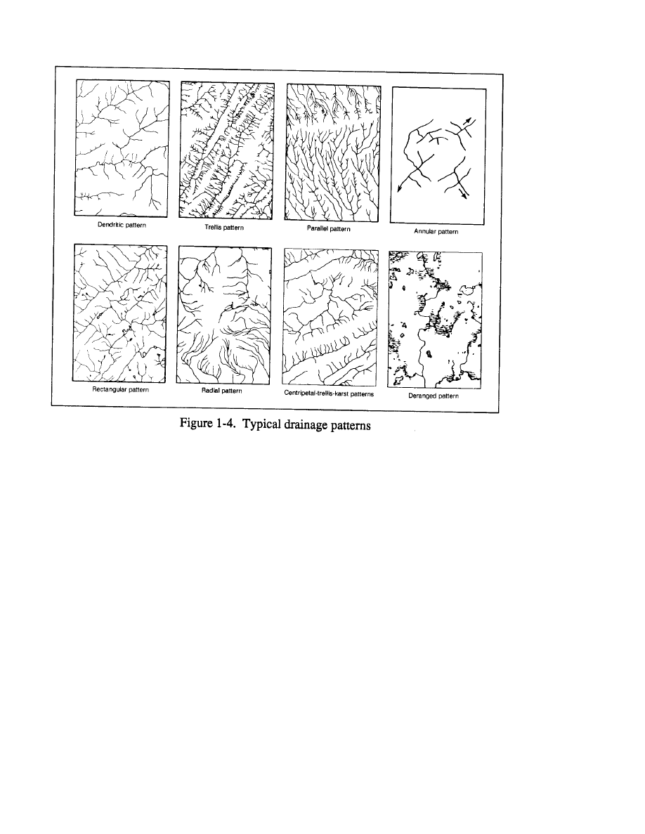
Patterns
The pattern of stream erosion usually gives an indication of rock structure and
composition and an indication of whether the region is underlined by one or several
rock types. The pattern can be dendritic, trellis, radial, annular, parallel, or
rectangular.
The dendritic drainage pattern is a tree-like pattern composed of branching
tributaries to a main stream, characteristic of essentially flat-lying and
homogeneous rocks. This pattern implies that the area was originally flat and is
composed of relatively uniform materials. Dendritic drainage is also typical of
glacial till, tidal marshes, and localized areas in sandy coastal plains. The dif-
ference in texture or density of a dendritic pattern may help identify surface
materials and organic areas.
In a trellis pattern, the mainstream runs parallel, and small streams flow and join
at right angles. This pattern is found in areas where sedimentary or metamorphic
rocks have been folded.
In a radial pattern, streams flow outward from a high central area. This pattern
is found on domes, volcanic cones, and round hills. However, the sides of a dome
or volcano might have a radial drainage system while the pattern inside a volcanic
cone might be centripetal, converging toward the center of the depression.
The annular pattern is a modified form of the radial drainage system, found where
sedimentary rocks are upturned by a dome structure. In this pattern, streams circle
around a high central area. The granitic dome drainage channels may follow a
circular path around the base of the dome when it is surrounded by tilted beds.
In the parallel pattern, major streams flow side by side in the direction of the
regional slope. Parallel streams are indicative of gently dipping beds or uniformly
sloping topography. The greater the slope, the more nearly parallel the drainage
and the straighter the flow. Local areas of lava flows often have parallel drainage,
even though the regional pattern may be radial. Alluvial fans may also exhibit
parallel drainage, but the pattern may be locally influenced by faults or jointing.
Coastal plains, because of their slope toward the sea, develop parallel drainage
overboard regions.
The rectangular drainage pattern is a specific type of angular drainage and is
usually a minor pattern associated with a major type such as dendritic. This pattern
is characterized by abrupt bends in streams and develops where a tree-like drainage
pattern prevails over a broad region. It is caused by faulting or jointing and is
generally associated with massive igneous rock. Metamorphic rock surfaces,
particularly those comprised of schist and slate, commonly have rectangular
drainage. Slate possesses a particularly finely textured system. Its drainage pattern
is extremely angular and has easily recognizable short gullies that are locally
parallel.
1-13
FM 5-33
Terrain Evaluation and Verification
PART ONE
Density
A determination of the density of the drainage pattern, or the number of streams
in a precise area, is very beneficial. The nature of the drainage pattern in an area
will provide a strong indicator of the particle size of the soils that have developed.
Surface sediments have good internal drainage. Sandstone, for example, due to
its porosity and permeability, has good internal drainage. Water can usually
percolate down through the soil and underlying reck, and the surface runoff will
beat a minimum. The texture or density of the drainage pattern that develops on
sandstone will be coarse.
A porous reek is not necessarily permeable. Clay, for example, contains up to 90
percent water arid is very porous but is not permeable because of the nature of its
flat-lying particles.
Sands and gravels are usually both porous and permeable, depending on sorting.
When precipitation occurs, some of the water can percolate down through the
sediment.
Shale is a relatively impermeable reek and has poor internal drainage. Surface
runoff will be at a maximum, and erosion will often be intense. The texture or
density of the drainage pattern that develops on shale will be fine-textured. See
Figure 1-4.
1-14

PART ONE
Terrain Evaluation and Verification
FM 5-33
OBSTACLES
Classification
An obstacle is any natural or man-made terrain feature that slows, diverts, or
stops the movement of personnel or vehicles. Obstacles are classified as natural,
such as escarpments, or man-made, such as built-up areas and cemeteries. They
are further categorized as existing-present natural or as man-made terrain features
that will limit mobility or as reinforced-existing features that man has enhanced to
use as obstacles, such as gentle slopes reinforced by tank ditches, pikes, or
revetments that limit mobility of maneuver units.
For classification purposes, obstacles must beat least 1.5 meters high and 250
meters long and have a slope greater than 45 percent (that which military vehicles
are unable to travel). Obstacles that will be delineated should be in areas where
they are of primary importance for the diversion of crosscountry movement.
Obstacles include escarpments, embankments, road cuts and fills, depressions,
fences, walls, hedgerows, and moats.
An obstacle factor overlay portrays linear terrain features that form natural
obstacles not normally identifiable on a topographic map. Obstacles located in
areas of dense forest, on steep slopes (greater than 45 percent), or within the gap
width of streams normally will not be shown on the obstacle overlay. Hydrologic
obstacles such as drainage ditches, channelized streams, and water banks are shown
on the surface drainage overlay.
Identification
Escarpments are terrain features similar to cliffs and ridges and appear on aerial
photographs as sharp breaks in the slope separating near level or gently sloping
surfaces. They are hazardous to both troop and vehicle movement due to the sharp
drop in the land typical of cliffs and ridges. Embankments are artificial structures,
usually of earth or gravel, constructed above natural ground surfaces such as dikes,
levees, and seawalls. Escarpments and embankments are tactically significant
because explosive devices can make the road, railroad, or cross-country route
impassable and because they can be used as channelization factors. This is
especially true if the bypass capability is restrictive to the state of the ground.
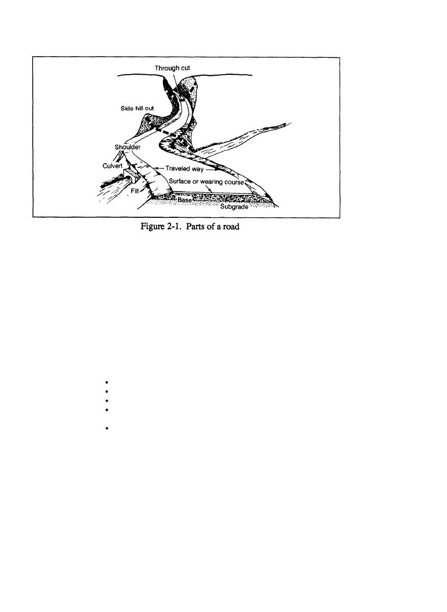
Railroad and road cuts and falls restrict military movement. Cuts are thorough-
fares or passages constructed through high areas. Fills are surfaces that have been
built up or raised to bring a low area up to the same level as the surrounding surfaces.
Depressions are low points or sinkholes surrounded by higher ground. They
usually have slopes equal to or greater than 45 percent, which will impede
movement across the terrain. Pits, quarries, and sinkholes are typical examples of
depressions.
Man-made features include fences or walls, hedgerows, and moats. Fences and
walls are usually constructed to separate or restrict crossings from one plot of land
to another. Hedgerows are tree-type barriers that can be identified by looking for
closely spaced rows of trees or bushes planted on a mound. They are so dense that
they restrict vehicle movement.
1-15

FM 5-33
Terrain Evaluation and Verification
PART ONE
European vineyards offer an excellent example of obstacles, due to the wet state
of the ground and the wire used to support crop growth. Combined with the existing
terrain, vineyards cause extreme difficulty in cross-country mobility.
Finally, moats are landforms that appear on photos as wide trenches or ditches
which usually surround a structure or prominent feature and are inaccessible to
vehicles. Moats are generally restricted to the British or European areas.
Preliminary identification can be made by referring to the map legend on a
topographic map.
1-16

PART ONE
Terrain Evaluation and Verification
FM 5-33
Man-Made Features
Chapter 2
URBAN AREAS
Urban-area intelligence is important in planning tactical and strategical opera-
tions, targeting for nuclear or air attack, and planning logistical support for
operations. Knowledge of characteristics in urban areas may also be important in
civil affairs, intelligence, and counterintelligence operations. Although informa-
tion is frequently accessible, the amount of detail required necessitates a substantial
collection effort.
The first aspect of urban intelligence includes geographic location, relative
economic and political importance of urban areas in the national structure, and
physical dimensions such as street shapes. The six street patterns are rectangular,
radial, concentric, contour conforming, medieval irregular, and planned irregular
(in the new residential suburbs of some countries).
The second aspect includes physical composition, vulnerability, accessibility,
productive capacity, and military resources of individual urban areas. Urban areas
are significant as military objectives or targets and as bases of operations. They
may be one or a combination of power centers (political, economic, military);
industrial production centers; service centers; transportation centers; population
centers; service centers (distribution points for fuels, power, water, raw materials,
food, manufactured goods); or cultural and scientific centers (seats of thought and
learning, and focal points of modem technological developments).
Buildings can provide numerous concealed positions for the infantry. Armored
vehicles can find isolated positions under archways or inside small industrial or
commercial structures. Thick masonry, stone, or brick walls offer excellent protec-
tion from direct fire, and ceilings for individual fire. Cover and concealment can
also be provided by the percentage of roof coverage. For detailed information, see
FM 90-10.
Although an urban overlay is not a standard product, it is useful for military
purposes. A subdivision can describe individual categories or break down a
division to more specific items as required by the user, as long as the subdivisions
are outlined in the legend. The division numbers in this manual are based on the
DFAD system, in PS/ICE/200. The first number describes the division as residen-
tial or industrial, the second number indicates the type of construction material,
2-1

FM 5-33
Terrain Evaluation and Verification
PART ONE
and the third number is the type of structure. If this number or its subdivisions are
not needed in particular overlays, the number will be followed by zeros.
The industrial category (code 100) consists of the area and facilities that include
the buildings used by those establishments engaged in the extraction, processing,
and production of intermediate and finished products or raw materials, The two
plant types in industrial areas are heavy manufacturing and medium and light
manufacturing. Heavy-manufacturing plants require distinctive structures, such as
blast furnaces, that could be readily recognized, while medium and light plants are
housed in general loft buildings from which machinery could be removed. The
specific type of medium-or light-manufacturing plant is not usually apparent from
the type of building.
The transportation category (code 200) consists of the area and facilities used in
moving materials and people on land. Features include railroads, roads, road
interchanges, bridges, bridge structures, and conduits.
The commercial/recreational category (code 300) consists of the area and build-
ings where the major business activities and recreational facilities comprise the
congested commercial core of a city. It includes retail and wholesale
establishments, financial institutions, office buildings, and hotels. Modem
multistory office buildings are typical of commercial sections of large cities.
More than one commercial area may exist, particularly in cities where a number of
towns have merged. Recreational activities, such as amusement parks and
stadiums, may also be present.
Residential areas of a city (code 400) consist of the area and associated buildings
where civilians live. They include many types of dwelling structures. Buildings
vary from one and two-story single family dwellings to multistory apartment
houses and may be built of any materials available locally. Types and sizes of
residential areas often indicate the number of people and the varying living
standards throughout the city.
Communication facilities (code 500) transmit information from place to place.
This category includes telephone, telegraph, and radio facilities, as well as other
electronic features such as power line pylons and structures. These facilities
include communication towers and buildings, as well as power transmission,
observation, microwave, television, and radio towers.
The governmental and institutional category (code 600) consists of the area and
facilities, primarily buildings, that constitute the seat of legal, administrative, or
other governmental functions of a country or political subdivision. This category
includes those buildings serving as public service institutions, such as universities,
churches, and hospitals. Governmental and institutional areas may include buildi-
ngs such as the capital; administrative centers such as ministries, departments,
courts, legislative buildings, embassies, and police headquarters; educational,
cultural, and scientific institutions such as schools, hospitals, universities, libraries,
museums, theaters, research institutions and laboratories; and religious and historic
structures such as churches, monuments, and shrines.
The military/civil category (code 700) consists of the area and facilities used by
the air, naval, and ground forces for waging war, training, and transporting
2-2

PART ONE
Terrain Evaluation and Verification
FM 5-33
nonmilitary goods and personnel by sea and air. Military areas usually include
transportation, billeting, storage, airfields, and administration facilities. Since
these are of strategic and tactical importance, they require as accurate a description
as possible for urban-area intelligence.
The storage category (code 800) consists of the area and facilities used for holding
or handling liquids or gases, bulk solids, and finished products. Examples are
cylindrical and spherical storage tanks; closed storage such as silos and grain bins;
open storage such as vehicle, ship, and aircraft storage areas and storage mounds
such as coal or minerals.
The landforms, vegetation, and miscellaneous features category (code 900)
describes the surface landscape characteristics or natural scenery features such as
levees, walls, and fences. It includes beaches, recreation areas, farms, wooded
areas, swamps, and vacant land. Extensive open areas within the city may be
valuable military assets, particularly if they have roads and railroad lines nearby
as well as access to electric and water supply facilities. Open areas on the outskirts
of cities arc the most immediately available land for military use. Features include
snow or ice areas, vegetation such as orchards and vineyards, agricultural areas,
and surface features such as embankments, fences, and cliffs.
TRANSPORTATION
Analysts preparing terrain studies must carefully evaluate all transportation
facilities to determine their effect on proposed operations. Analysts may recom-
mend destroying certain facilities or retaining them for future use. The entire
transportation network must be considered in planning large-scale operations. An
area with a dense transportation network, for example, is favorable for major
offensives. Networks that are criss-crossed by canals and railroads and possess
few roads will limit the use of wheeled vehicles and the maneuver of armor and
motorized infantry.
The transportation facilities of an area consist of all highways, railways, and
waterways over which troops or supplies can be moved. The importance of each
area depends on the nature of the military operation involved. An army’s ability
to carry out its mission depends greatly on its transportation capabilities and
facilities.
Highways
Features
Military interest in highway intelligence of a given area or country covers all
physical characteristics of the existing road, track, and trail system. All associated
structures and facilities necessary for movement and for protection of the routes,
such as bridges, ferries, tunnels, and fords, are integral parts of the highway system.
Planners must know where new routes will be needed to support an operation.
Road widths are given in meters. Measurements indicate the minimum width of
the traveled way. Each road segment between intersections is assigned a width
value, and that number is placed parallel to the road segment.
The severe abuse given to roads by large volumes of heavy traffic, important
bridges, intersections, and narrow defiles makes them primary targets for enemy
2-3
FM 5-33
Terrain Evaluation and Verification
PART ONE
bombardment. Planners must avoid maintaining unnecessary routes and must hold
construction of new routes to a minimum.
Road Classification
Five road classifications are recognized on 1:50,000 scale topographic maps.
They are all-weather, hard-surface dual/divided highway; all-weather, hard- sur-
face highway; all-weather, loose-surface highway; fair-weather, loose-surface
highway; and cart track.
All-weather, hard-surface, dual/divided highways normally have waterproof
surfaces paved with concrete, bituminous surfacing, brick, or paving stone and are
only slightly affected by precipitation or temperature changes. The route is never
closed to traffic by weather conditions other than temporary snow or flood
blockage. Photo interpretation keys include:
Traveled portion of roadway is fairly straight.
Even curves are present.
Road width is uniform with easily seen parallel sides.
Photo tint of mad surface is an even color and varies from dark gray to
white.
Absence of ruts or holes on traveled portion of the roadway.
All-weather, hard-surface highways have waterproof surfaces of concrete,
bitumen, brick, or paving stone and are only slightly affected by rain, frost, thaw,
and heat. They are passable throughout the year to a volume of traffic never
appreciably less than its maximum dry-weather capacity. They are never closed
by weather conditions other than temporary snow or flood blockage. Photo
interpretation keys are similar to those for the dual or divided highway.
All-weather, loose-surface highways are not waterproof but are graded and
drained and are considerably affectedly rain, frost, or thaw. They are constructed
of crushed rock, water-bound macadam, grovel, broken stone and cinders, or
2-4

PART ONE
Terrain Evaluation and Verification
FM 5-33
smoothed earth with an oil coating. The roads are kept open in bad weather to a
volume of traffic considerably less than its maximum dry-weather capacity. Traf-
fic may be halted for short periods of time. Heavy use during adverse weather
conditions may cause complete collapse. Photo interpretation keys include:
Sharp or irregular curves are present.
Roadway meanders to avoid steep slopes.
Gravel or crushed rock appears a uniform light gray except for low spots
that collect water and appear in dark tones.
Ruts and stones give the roadway a mottled appearance.
Roadway edges and shoulders are not clean, sharp lines; sometimes, they
are very difficult to determine.
Fair-weather, loose-surface highways are constructed of natural or stabilized soil,
sand clay, shell, cinders, or disintegrated granite or rock. They include logging
roads, abandoned roads, and corduroy roads which become quickly impassable in
bad weather. Photo interpretation keys are similar to those for the all-weather,
loose-surface highway except for less visible maintenance and narrower road
widths at stream crossings.
Cart tracks are natural traveled ways including caravan routes and winter roads.
They are not wide enough to accommodate four-wheeled military vehicles. Photo
interpretation keys include
Irregular turns and bends.
Traveled roadway width varies.
Apparent lack of direction.
Roadway detours around wet terrain.
Railroads
Railways are a highly desirable adjunct to extended military operations. Their
capabilities are of primary concern and are the subject of continuing studies by
personnel at the highest levels.
Railroads include all fixed property belonging to a line, such as land, permanent
way, and facilities necessary for the movement of traffic and protection of the
permanent way. They include bridges, tunnels, snowsheds, galleries, ferries, and
other structures.
Commanders need information on physical characteristics to determine railway
capacities and maintenance or rehabilitation requirements. Railway intelligence
covers all physical characteristics of the existing system and all available informa-
tion pertaining to development, construction, and maintenance. Physical charac-
teristics describe the railroad and its critical features and component parts such as
roadbed, ballast, track, rails, and horizontal and vertical alignment.
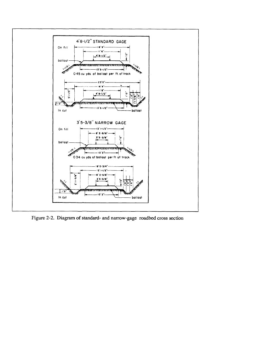
Identification Keys
Railroads have definite characteristics distinguishing them from roads and high-
ways (see Figure 2-2). Railroads often follow rivers, to take advantage of the
normal gradual gradient of the valley. They follow as straight a line as possible,
while roads meander. Curves are usually long and smooth, while roads may have
sharp, right-angle turns and T-shaped intersections.
2-5
FM 5-33
Terrain Evaluation and Verification
PART ONE
Gradients are as level as possible and seldom exceed more than three or four
percent, while roads often have steep grades. In order to keep gradients at a
minimum, many cuts and fills exist along the right-of-way, especially in rolling or
broken terrain, while roads run up and down hills with fewer cuts and fills.
Few houses are found along railways. Highways and railroads cross each other
in such a manner that no interchange of traffic is possible. Grade crossings have
distinct intersection angles, and overpasses and underpasses are obvious.
The gage of a railroad is the distance between the rails. Knowledge of railroad
gages is useful to image interpreters for determining photo scales. Also, knowing
that a change in gage may occur at an international border, the interpreter should
look for transshipment stations. Railroad gages are classified as wide, standard, or
2-6

PART ONE
Terrain Evaluation and Verification
FM 5-33
narrow. Wide gages are 5 feet or wider. They are mostly used by Russian, Finnish,
and Spanish lines. Standard gages are 4 feet, 8½ inches. They are used for main
and branch lines in the United States and the rest of Europe. Narrow gages are less
than standard. Their use is somewhat limited to and usually found in mountainous,
industrial, logging, and coastal defense areas and in mines and supply dumps. In
South and Central America, the one-meter gage is found in many places; however,
many of the countries are now adopting the standard gage because they import
US-made rolling stock. See Figure 2-2.
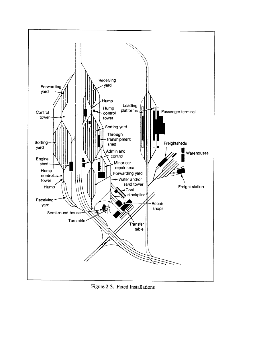
Fixed Installations
Classification (marshaling) yards are used to sort freight cars. They are identified
by a large group of parallel tracks with a restricted (one-or two- track) entrance
and exit called a choke point. Active classification yards include numerous freight
cars and small switch engines. Two or more classification yards are frequently
found next to each other, with their entrances through a choke point. If this choke
point is higher than either classification yard, it is known as a hump. Also, one
yard is often placed slightly higher than the neighboring yard to allow cars to coast
out of one yard through the choke point into a previously selected track of the other
yard.
Service yards are normally found in or near marshaling yards and can be
identified by the presence of roundhouses, turntables, service facilities, and car
repair shops. Roundhouses are used for light repair and storage of locomotives.
The number of roof vents on top of the roundhouse indicates the capacity of the
roundhouse. Turntables are used for turning the engines around. Service facilities
include coal towers, water towers, and coal piles. Car-repair shops normally appear
as long, low buildings straddling one or more tracks, with cars awaiting repairs on
sidings adjacent to the buildings.
Freight or loading yards are identified by loading platforms, freight stations,
warehouses, and access to other means of transportation. Special loading stations
are identified by grain elevators, coal and ore bins, oil storage tanks, and livestock
pens with loading ramps.
Passenger stations vary from small rural depots or suburban stations to large
stations and terminals. Small stations usually do not have loading docks and may
not have parking areas for automobiles or trucks. They are located close to a track,
and shelters may cover waiting platforms if more than two tracks pass the station.
Large stations are identified by a large number of tracks leading into or past a large
building that houses waiting rooms, ticket offices, and other passenger facilities.
The track or boarding area is normally covered.
Freight stations may be identified by loading docks along railroad tracks on one
side of a building and loading docks along a road or street on the opposite side.
Freight stations are small, single structures near passenger stations designed for the
temporary storage of goods received. Warehouses may be away from fixed railroad
installations, and more than one may be located in an area. Freight cars loading or
unloading at a freight station aid in identification of the installation. See Figure
2-7
FM 5-33
Terrain Evaluation and Verification
PART ONE
2-8

PART ONE
Terrain Evaluation and Verification
FM 5-33
Rolling Stock
Locomotives.
Locomotives vary greatly, from small switch engines 24 to 30 feet
long m mainline passenger and freight locomotives 35 to 50 feet long. Locomo-
tives longer than 50 feet are used for special purposes such as mountain climbing.
Locomotives may be steam, electric, diesel, or diesel-electric. Steam locomotives
are easily identified by smoke and stream around an operating locomotive, a
smokestack, and a fuel tender attached just behind the locomotive. Electric
locomotives have no fuel tender or smokestack and may be identified by overhead
antennae if they receive their power from overhead lines. The lines may be
evidenced by the shadows their support poles cast. Diesel locomotives lack a fuel
tender and are usually identified by their streamlined appearance.
Freight cars.
The boxcar is the most frequently found freight rolling stock,
recognized by its rectanglar shape and little roof detail. The round-topped freight
car differs only in its top. These cars average 40 to 45 feet in length in the US, 25
feet in Europe. Other freight cars are the gondola and hopper cars, which are used
for coal, ore, and other bulky material or large freight that cannot be loaded into a
boxcar. Shape and shadow aid in identification. Refrigerator, stock, and
automobile cars are so close in appearance to boxcars that low-level obliques arc
usually necessary to distinguish them. Cabooses, not always found on foreign
railroads, appear as small cars attached to the end of freight trains, usually with a
visible cupola.
Passenger cars.
For identification purposes, the outstanding characteristic of
passenger cars is their length, especially when compared with freight cars. They
vary from 50 to 80 feet. Normally, it is not possible to distinguish a coach from a
sleeping or dining car.
Special Equipment.
Railroads have a variety of special equipment in their
rolling stock. The railcar is a self-contained unit with its own power plant as well
as space for passengers or mail and baggage or all three. Cranes, snowplows, and
drop-center flatcars are sometimes present on rolling stock.
Railheads
Railheads are points of supply transfer from railroads to other transportation and
are generally found in small towns or cities where sidings and storage space already
exist. Characteristics of a railhead are spurs and sidings from a main line; a road
net, including narrow gage railroads, leading away from the area; piles of materials
stacked near the track trucks or wagons or both, either without order or organized
into convoys or trains; and temporary dwellings, such as tents or Quonset huts, for
housing troops guarding and handling supplies.
End Points
System.
A railroad system is a network of railroads operated by a single
management entity, government or corporate. System end points are the points
where a railroad system begins, ends, or changes identification. There may be no
system end points within many map sheets, but system end points will always
coincide with route and segment end points.
Route.
A route is the portion of a system providing through lines between
selected points. Routes are usually specified by the system management, but it
2-9

FM 5-33
Terrain Evaluation and Verification
PART ONE
may often be convenient or appropriate for the analyst to select others. The route
will be identified on the factor overlay by abbreviations of the two endpoints placed
in parentheses. There may be no route end points within the area of a 1:50,000
factor overlay. Route end points always coincide with segment end points and may
coincide with system end points. Kilometer distances are always measured from
route end points.
Segment.
A segment is the portion of a route characterized by uniform load-bear-
ing, traffic capacity, and operating characteristics. Analysts will number segments
sequentially along a route within a map sheet, starting at the segment nearest the
zero kilometer point. End points of segments are defined by nodes along the route,
at which anyone of the following conditions occurs:
A change in the number of tracks (points where passing tracks or sidings
start or end do not constitute nodes).
A change in the gage of the track.
A route or system terminal.
The point where the route crosses the neat line of the factor overlay.
A terminal or junction where traffic may be diverted onto another route.
A change in the type of construction such that the load-bearing capacity,
speed or traffic capacity is altered.
A point where electrification starts, ends, or changes method of power
transfer.
A point where a change in traffic control methods occurs, such as intern-
ational boundary crossings.
Number of Tracks
Analysts indicate the number of tracks for single- and double-track lines by the
number of ticks used with the gage symbol. Routes with three or more tracks are
symbolized by the double-track symbol supplemented by a T and a number, which
indicates the actual number of tracks. Lines operated by different systems that
closely parallel each other or share a common right-of-way are in juxtaposition
(side by side) and are indicated by separate symbols. Symbols for such lines will
be sufficiently displaced from the centerline to make it clear that two distinct lines
exist.
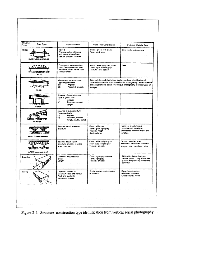
Bridges
Features
Structures and crossings on highways or railways include bridges, culverts,
tunnels, galleries, ferries, and fords. For the purpose of terrain intelligence, they
also include cableways, tramways, and other features that may reduce or interrupt
the traffic flow on a transportation route. Bridges and culverts are the structures
most frequently encountered; however, any feature that may present a potential
obstacle is significant in a military operation. See Figure 2-4.
Any type of structure or crossing on a transportation route is an important portion
of the route regardless of the mode of transportation. Maps, charts, photographs,
and other sources contain valuable information that analysts should exploit.
Highway and railway bridges and tunnels are vulnerable points on a line of
communications. Information about prevention, destruction, or repair of a bridge
may be the key to an effective defense or the successful penetration of an enemy
2-10
PART ONE
Terrain Evaluation and Verification
FM 5-33
2-11
FM 5-33
Terrain Evaluation and Verification
PART ONE
area. A bridge seized intact has great value in offensive operations, since even a
small bridge eases troop movement over a river or stream.
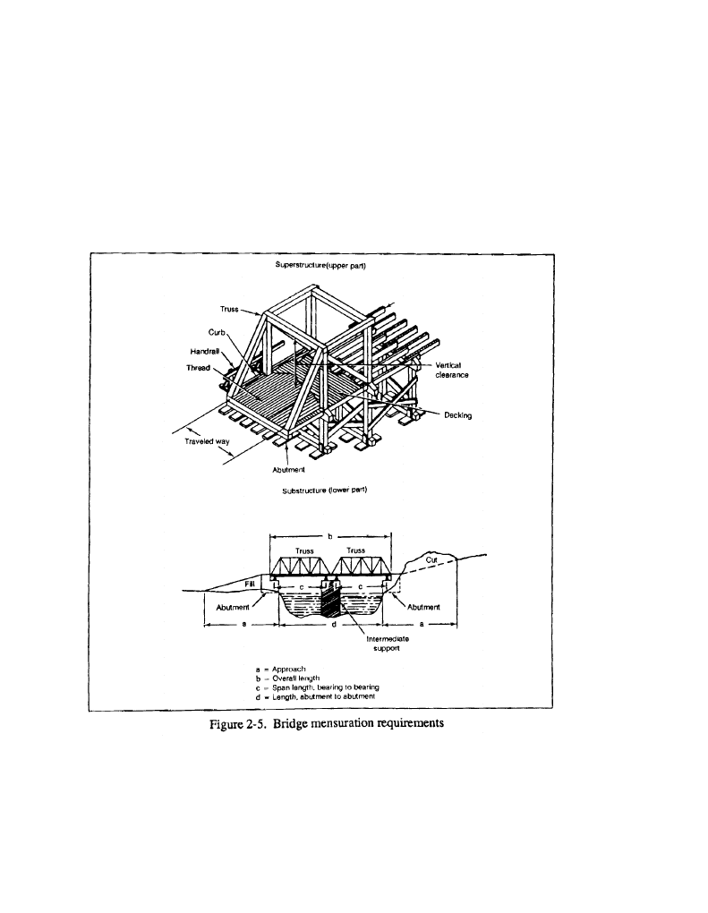
A bridge includes the substructure and superstructure. The substructure com-
prises the foundation and supporting elements of a bridge; the superstructure is the
assembly that rests on the substructure and spans the gaps between ground supports.
Bridge superstructures take many forms, ranging from short trestle spans built
into wooden stringers to large multiple cantilever spans of several thousand feet.
Most have two basic components, the main supporting members and a floor or deck
system. The primary exception is the concrete slab design, in which the supporting
member also serves as the floor. The superstructure used depends on the loads to
be carried, required span lengths, time available for erection, availability of
2-12

PART ONE
Terrain Evaluation and Verification
FM 5-33
construction materials, manpower and equipment, and characteristics of the site.
Based on their superstructures, bridges may be either fixed or movable. The five
major categories of fixed bridges are beam, slab, girder, truss, and arch bridges.
These types may occur alone or in combination. Movable bridges have at least one
span that can be moved from its normal position to allow passage of vessels. The
four general types of movable bridges are swing, lift, bascule, and retractile.
The load capacity is the most critical factor of abridge. The most reliable capacity
data comes from the standard design loadings by which most countries design their
bridges. Usually a country has a number of standard design loadings for different
capacity classes. Standard design loadings may be expressed by a letter, number,
or symbol.
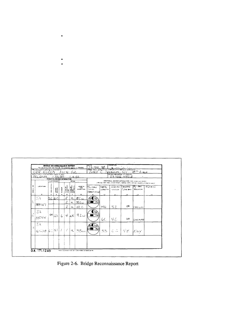
Bridge Reporting
The data base includes all-on route bridges that can be identified and measured
on aerial photography or derived from updated collateral sources. Structures less
than 6 meters long are culverts; all others are treated as bridges. This cut-off
length is flexible according to the prevalence of bridging in the study area.
All bridges present a potential restriction to traffic, and all items reflected in the
collection checklist are important. Some of the basic requirements for informa-
tion on any type of bridge are--
Location, or kilometer stations from origin of section. The nearest
kilometer should be given unless close spacing requires use of the nearest
0.1 kilometer for separate identifications.
Obstacle crossed. Analysts must list the name of the stream when they
know it. Other possible entries include gorge, railroad, and canal.
Universal transverse mercator (UTM) coordinates to six places and
geographic coordinates to the nearest second.
Overall length, to the nearest meter. This should generally be the sum of
the span lengths, but it should not include approaches.
Roadway width to the nearest 0.1 meters of that portion of the deck over
which vehicles normally run, excluding sidewalks, curves, parapets, truss
superstructure, and so forth. Width is measured between the inside faces
of the curbs.
Horizontal clearance, or the limiting width to the nearest 0.1 meter at a
point 30 centimeters above the edge of the roadway. This normally in-
cludes widths of curbs and sidewalks but excludes parapets and trusses.
The horizontal clearance on a truss bridge is measured from a point 4 feet
above the roadway.
Vertical clearance, or the minimum distance between the roadway and
any obstruction immediately over the roadway, to the nearest 0.1 meter.
The letter u, for unlimited clearance, indicates no obstruction.
Military load classification (MLC). This number indicates the carrying
capacity of the bridge, including classifications for single- and double-
flow traffic. The symbol to show the MLC is a circle with the bridge in-
formation on the inside. The load classification is on the top of the circle.
In those instances where dual classifications for wheeled and tracked
2-13
FM 5-33
Terrain Evaluation and Verification
PART ONE
vehicles exist, both classifications are shown. See TM 5-312 for further
information. See the NATO bridge symbol on Figure 2-6.
Spans. Both the number and length of spans need to be determined.
Lengths are given to the nearest 0.1 meter and represent the distance
between supports, or centers of bearing. The bridge classification is
measured fron center to center of supports and is based on the weakest
span.
Span construction. The construction material and type will be identified.
Bypasses. Bypasses are local detours along a specified route that enable
traffic to avoid an obstruction. They are classified as easy, difficult, or im-
possible according to the ease of access to the bridge bypass. See Figure
2-6.
Culverts
Culverts are grouped into four main categories of pipe, box, arch, and rail girder
spans. Pipe culverts are the most common. They are usually concrete, but
corrugated metal and cast iron are also used. The pipes have different shapes and
range from 12 inches to several feet in diameter. Box culverts are used to a great
extent in modem construction. They are rectangular in cross section and usually
concrete. A large box culvert is similar to a slab bridge. Arch culverts were used
frequently in the past but are rarely constructed now. They are concrete, masonry,
brick, or timber. Rail girder spans are found on lightly built railways or, in an
emergency, on any line. The rails are laid side by side and keyed head to base and
may be used for spans of 3 meters or less.
Tunnels, Galleries, and Snowsheds
Features on a transportation route where it would be relatively easy to block traffic
or that affect the traffic capacity of the road are critical. Such features include
2 - 1 4
PART ONE
Terrain Evaluation and Verification
FM 5-33
tunnels, snowsheds, and galleries. These obstructions can prevent access to
vehicles with certain physical dimensions. Reductions in traveled-way widths,
such as narrow streets in built-up areas, drainage ditches, and embarkments, can
also limit vehicular movement. This is an important aspect of transportation
intelligence.
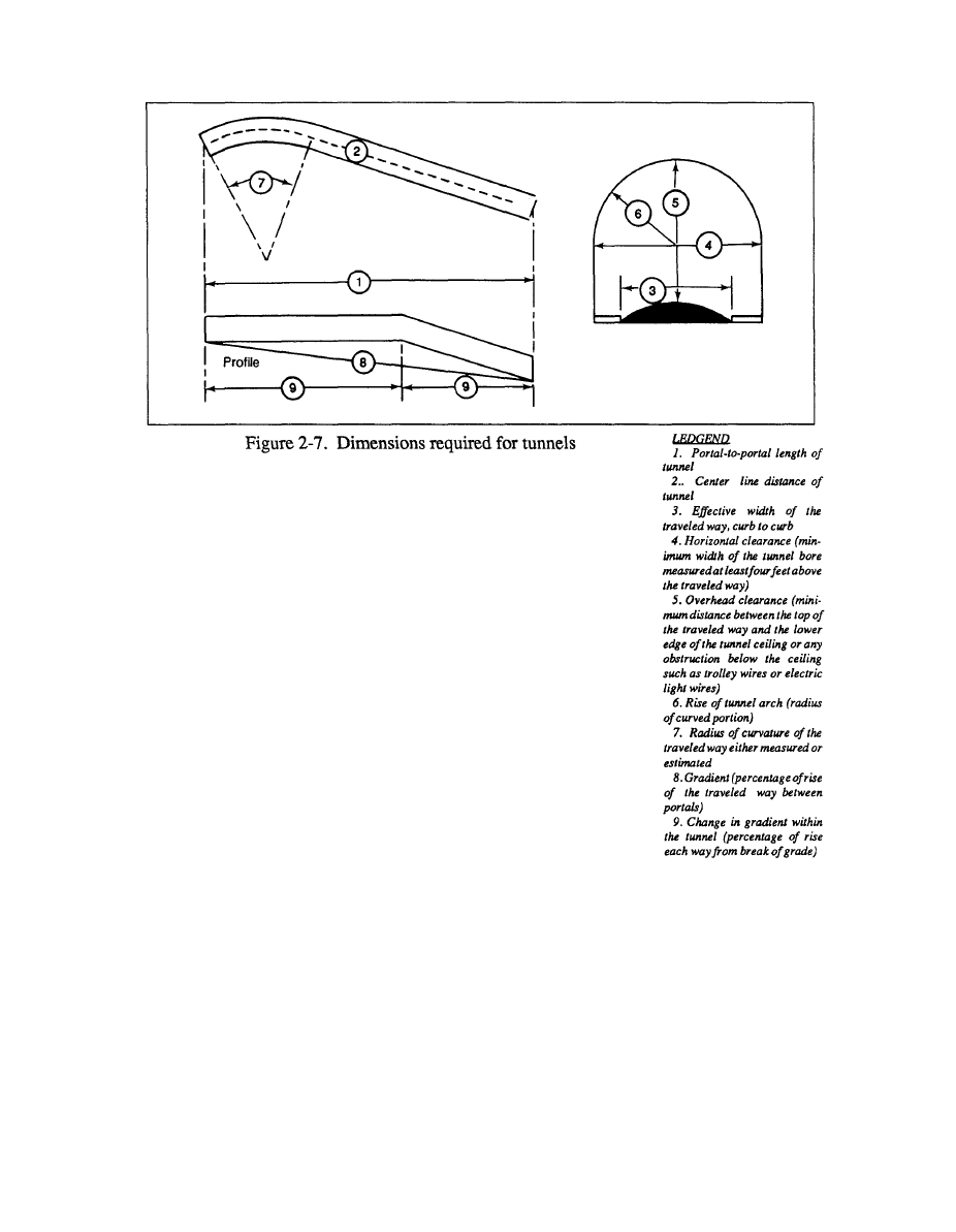
Tunnels
A tunnel is an underground section of the route that has been bored or made by
cut-and-cover for a route passage. It consists of the bore or bores, portals, and
possibly a liner. Tunnel bores are commonly semicircular, elliptical, horseshoe, or
square with arched ceiling. Bores may be lined with brick, masonry, or concrete,
or they may be unlined. Some very long tunnels on steam-operated railroad lines
are artificially ventilated by blowers at the portals or in ventilating shafts above the
bore. Alignment of tunnels may be straight or curved. See Figure 2-7.
Galleries and Snowsheds
Built in rugged, mountainous terrain, these protective structures are not as
common as bridges or tunnels. Galleries offer protection against snow and rock
avalanches. They may be cut into the side of a cliff and have a natural overhang,
or the cover may be a concrete slab, either of which guides the avalanche across
the track or road. One side of a gallery is usually open. Snowsheds offer protection
against snow accumulations and slides on exposed sections of the permanent way.
Ferries
Ferries or ferry boats convey traffic and cargo across a river to another water
barrier. These vessels vary widely in physical appearance and capacity depending
on the depth, width, and current of the stream and on the characteristics of traffic
to be moved. Propulsion of ferries may be by oars, cable and pulleys, poles, or
stream current such as trail and flying ferries, or by steam, gasoline, or diesel
2-15

FM 5-33
Terrain Evaluation and Verification
PART ONE
engines. Construction of ferry boats varies widely from expedient rafts to ocean-
going vessels.
The capacity of a ferry boat is usually expressed in tons and total number of
passengers and is sometimes assigned an MLC number. When more than one ferry
is employed for a given site, report the capacity of each.
Climatic conditions have a marked effect on ferry conditions. Fog and ice
substantially reduce the total traffic-moving capacity and increase the hazard of the
water route. Therefore, data on tide fluctuations, freezing periods, floods, exces-
sive dry spells, and their effects on ferry operations is important.
A ferry site is the place where ferries convey traffic and cargo. Ferry slips or piers
are generally provided on the shorn to permit easy loading. The slips may vary
from simple log piers to elaborate terminal buildings. A common characteristic of
ferry slips is a floating or adjustable approach ramp that accommodates variations
in ferry deck level. Analysts must consider the limiting characteristics of ferry
sites, such as the width of the water barrier from bank to bank, the distance and
time traveled by the ferry boat from one side to the other, and the water depth at
each ferry slip.
Approach routes to ferry sites have an important bearing on ferry use. Analysts
should report the condition of the approaches, including the load-bearing capacity
of landing facilities.
Fords
A ford is a location in a water barrier where the current, bottom, and approaches
permit the passage of personnel or vehicles and other equipment, where little or no
swimming is required, where they cross under their own or assisted propulsion, and
where their wheels or tracks remain in contact with the bottom.
Fords are classified according to their crossing potential, or trafficability, for foot
or wheeled and tracked vehicles. Fordable depths for vehicular traffic can be
increased by suitable waterproofing or, in the case of modem tanks, by adding
deep-water fording kits that permit fording depths up to 4.3 meters.
Approaches may be paved with concrete or bituminous surface material but are
usually unimproved. Analysts should carefully note the composition and slope of
approaches to a ford to permit determination of trafficability during inclement
weather and after fording vehicles have saturated surface material.
Bottom conditions are determined by checking the stability and composition of
the bed. The composition of the stream bottom determines its trafficability. In
some cases, the natural river bottom of a ford may have been improved to increase
load-bearing capacity and to reduce the water depth. Improved fords may have
gravel or concrete surfacing, layers of sandbags, metal screening or matting, or
timber or wooden planking.
Climatic conditions such as seasonal floods, excessive dry seasons, freezing, and
other extremes of weather materially affect stream foldability. The velocity of the
current and the presence of debris also affect the condition and passability of a ford.
2-16

PART ONE
Terrain Evaluation and Verification
FM 5-33
Current estimates are swift (more than 1.5 meters per second), moderate (1 to 1.5
meters per second), and slow (less than 1 meter per second).
Low-water Bridges
Low-warm bridges consist of two or more intermediate supports with concrete
decking and are located whoIly within ravines or gullies. During high-water
periods, they may easily be confused with paved fords, as both are completely
submerged. Because of corresponding military load limitations, analysts must
properly identify low-water bridges and paved fords.
Cableways and Tramways
Cableways, tramways, and so forth are not usually major factors in a military
operarion; however, they may be encountered in rugged mountainous regions and
beach areas or used as connections between two primary supply routes. In some
cases they may extend for several miles and be the best available method for
moving supplies.
Pipelines
Pipelines
that carry petroleum and natural gas represent an important mode of
transportation. White rail, water, and road transport are used extensively for
transporting fluids and gases, the overland movement of petroleum and refined
products is performed most economically and expeditiously by pipeline. Crude-oil
pipelines are used only to transport crude oil, while many refried-product pipelines
carry more than one product. These products are sent through the pipelines in
tenders, or batches, to keep the amount of mixing to a minimum. Because of their
most vital link in an industrialized country’s energy supply system, coal and ore
are also carried in pipelines as slurry.
Components
Pipes are used in long-distance pipelines and in many local lines. They are
composed of welded steel with diameters varying from 15 centimeters to more than
1 meter, depending upon the economies of the line’s construction. The pipe may
be Iaid either underground or above grorrnd and may extend cross-country or follow
the alignment of roads and railroads. When a pipeline must cross a stream, the
pipes are usually laid along the stream bottom. Where streams are swift or where
beds may shift rapidly, either the pipe is attached to existing bridges or special
pipeline suspension bridges are built. Siphon crossings are used where necessary,
When an
increase or decrease of pressure is required, regulating features such as
pumps or compressors are used. Pumping stations are used for liquid fuels and
compressor stations for gas. They are similar in appearance except for the cooling
towers present at compressor stations.
Valves, manifolds, and meters are integral parts of any pipeline system and are
located at frequent intervals along the pipeline and at terminals. Valves protruding
from the ground are often the only indicators of a pipeline alignment.
2-17
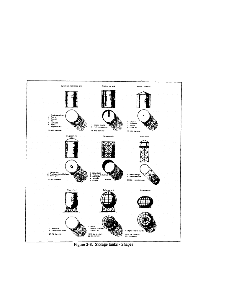
FM 5-33
Terrain Evaluation and Verification
PART ONE
Terminal Facilities
Refinery terminals consist of numerous tanks for the separate storage of crude oil
and refined products. Facility size and type depends on whether the refinery is
located near the source of supply or consuming center, Refined-product dispensing
terminals contain a variety of products for final distribution.
-
-
-
Natural gas is generally stored in bulk, below the ground, and under high-pressure,
Large underground gas storage pools, usually caves or quarries near consuming
centers, are often used to store gas for seasonal or emergency needs. Above ground,
natural gas is stored mostly under pressure in spherical tanks, but large telescoping
tanks are sometimes used for low-pressure storage. Natural-gas receiving ter-
minals are located at the producing field and contain facilities for conditioning the
gas for pipeline transmission. Natural-gas dispensing terminals are located at
2-18
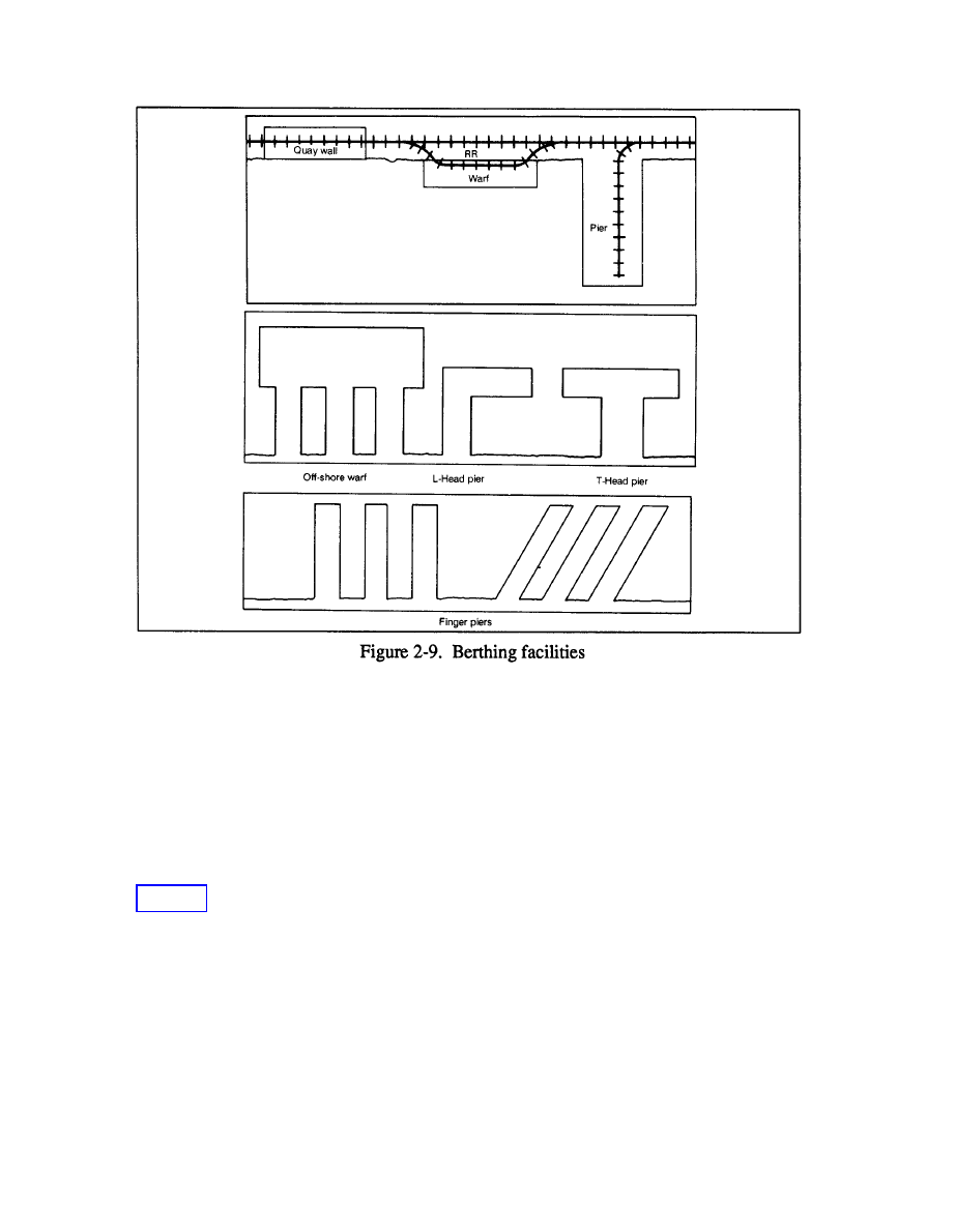
PART ONE
Terrain Evaluation and Verification
FM 5-33
consuming centers and include dispatching and metering facilities and sufficient
storage facilities to meet peak demands.
Storage tanks, found in varying numbers at all petroleum installations, are easily
recognized. Volatile products such as gasoline and kerosene are generally stored
in floating roof tanks. These tanks have roofs that float on the liquid to reduce
space in which vapor might form. Nonvolatile products such as fuel oils and crude
oil are stored in fixed-roof tanks. Petroleum gases are generally liquefied and
stored under pressure in spherical tanks or in horizontal cylindrical tanks. The
number and variety of tanks in a storage installation indicate the quantity and types
of product stored. Areas of great extent and capacity are called tank farms. See
PORTS AND HARBORS
Information about ports, naval bases, and shipyard facilities is essential for
estimating capacities, vulnerability, and other items of military significance.
Ports
Ports are settlements with installations for handling waterborne shipping. Prin-
cipal port facilities are berthing space, storage space, cargo-handling equipment,
cargo transshipment facilities, and vessel-servicing facilities. Ports are classified
on an areawide rather than a worldwide basis, and a principal port in a small
2-19
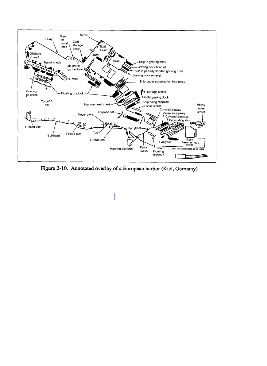
FM 5-33
Terrain Evaluation and Verification
PART ONE
maritime nation may be equivalent to a much lesser port in the more extensive port
system of another country. In wartime, principal and secondary ports and bases
are prime targets for destruction, and the relative importance of minor ports
Ports may have various structures affording berthing space or may be anyplace
a vessel may be made fast. These structures include piers, moles, and wharves or
quays. Perhaps the most important difference between these structures is that piers
are supported by pilings driven into the harbor bottom, while moles are of solid
construction. In addition, wharves and quays are parallel with the shoreline, while
piers and moles are perpendicular to it.
Harbors
Harbors are areas where the anchorage and shore are protected from the sea and
storms by natural or man-made barriers. Areas that do not have this protection but
are still suitable for vessel anchorage are open anchorages or roadsteads. A good
harbor must have deep water, adequate protection from storms, enough space to
accommodate large numbers of vessels, and a shoreline that can be developed as
a port and as a site for industry. Harbors may be situated on the sea, estuaries, or
inland lakes and rivers and may easily be recognized by abundant waterborne traffic
and port facilities. See Figure 2-10.
Relatively few strategically located natural harbors are large enough or safe
enough to be valuable to shipping. Many of the important harbors of the world are
man-made. Most harbors have some or all of the more common artificial protective
2-20

PART ONE
Terrain Evaluation and Verification
FM 5-33
structures. A breakwater is a massive stone or masonry structure extending across
or at an angle to the entrance to the harbor. A jetty is the name applied to a
breakwater that connects with the shore. A mole is a jetty that is wide enough to
allow construction of a roadway along the top. A sea wall is a structure built along
the coastline to prevent the sea from eroding the land.
Within the harbor itself are various types of buoys used as navigational aids. In
addition, lighthouses, mooring buoys, and dolphins are often present. Mooring
buoys are huge buoys located in the harbor so that vessels may tie up without
dropping anchor. Only when a harbor has been developed for transacting business
between ship and shore does it become part of a port. Dolphins are groups of pilings
driven into the harbor bottom for the same purpose.
Dolphins usually consist of a cluster of piles lashed together at the top. They are
located off shore and are used singly for mooring into or hauling out of a berth and
in a series for mooring a ship alongside. Dolphin moorings conserve space in the
stream and are used either for idle berthing or for loading cargo from lighters.
Dolphins are often associated with a wharf either as a protective device at wharf
corners or as a means of increasing the length of berthing space provided by a wharf
face.
A dock, also called a slip or berth, is the water adjacent to a mole, pier, or wharf
when that water area is narrow and affords berthing space. Basins are broad and
expansive, artificially enclosed bodies of water that form a harbor or part of a
harbor. They may be tidal basins in which water is subject to tidal influences, or
controlled-level basins in which the water level is maintained irrespective of tidal
change. Controlled-level basins are either wet docks or half-tide basins. A wet
dock is enclosed by a gate, caisson, or lock. It may be filled by naturally
impounding water at each high tide or at spring tides only. Pumping plants may
be provided for initial filling or for elevations of the water above that achieved by
natural impounding. The half-tide basin has gates at each end and is used in much
the same manner as a large leek to increase the enormous amount of water required
to raise the water level. It cannot be used at all states of the tide.
Harbor works, including protective works, are structures designed to provide
shelter, control water flow, and regulate erosion for improvement of the
navigability of a harbor. The principal structures are breakwaters, jetties, groins,
sea walls, bulkheads, dikes, locks, and moles. Harbor works do not include port
facilities that are designed specifically for transfer of cargo and the servicing ships.
Depths are important in such port topics as harbor, entrance, anchorage, wharves,
and dry docks. They are computed in terms of established reference planes that
are based on but do not necessarily coincide with tidal levels. The particular
reference plane on which depths on a hydrographic chart are based is called chart
data and is defined on the chart. Precise data is established for most ports and is a
basis for soundings. Analysts should clearly indicate the reference plane when
reporting depths.
The navigable waterways through the approach, the entrance to the harbor, and
the harbor itself frequently determine the size of the ships (draft, length, beam,
height above water) that can be accommodated in the port. Analysts should
describe in detail any thruway with controlling dimensions that limit the size of
2-21

FM 5-33
Terrain Evaluation and Verification
PART ONE
ships which can traverse it. Reports on the experiences of ships with critical
dimensions that have entered are most helpful.
Cranes (Cargo-handling Equipment)
Cargo berthing space may be recognized by the presence of heavy handling
equipment located on piers or wharves. However, very small ports may not have
any such equipment, requiring vessels to supply and use their own. Port cargo-
handling equipment includes various hoists for handling general cargo and special
equipment for other cargo.
A gantry crane is a traveling crane on rails that consists of a hoist on a heavy cross
girder supported at two points. Hoisting is performed by a trolley or crab that
moves transversely along the bridge. Gantry cranes occasionally serve as a base
for a jib crane, the latter being mounted on and capable of transverse movement
along the bridge member. They are used extensively in shipyards for hull erection
and in various industrial yards and shops for heavy lifting. They are almost always
electrically operated. Depending on use, they may range up to 250 tons capacity.
Hoisting capacity is constant regardless of the position of the crab or trolley on the
bridge.
A cantilever crane consists of a base or tower structure on which is mounted a
counterbalanced horizontal arm or jib. A trolley that can be racked along rails on
the cantilevered jib carries the hoisting sheaves. The trolley does not carry the
hoisting mechanism but merely serves to support the fall, and its transverse
movement is controlled by a system of sheaves and ropes. Cantilever cranes are
most commonly found in shipyards, although they may be used for cargo handling
in special instances where a large working radius is required. They are normally
electrically powered and range up to 250 tons or more in capacity. Capacities
should be reported at maximum and minimum radius. One type of cantilever crane
is the hammerhead. These cranes are supported at one point, about which the
mechanism can turn. The hoisting end is balanced by a cab or counterweight. The
entire machine may be mounted on rails for movement along the pier or wharf.
A jib crane consists of the primary arm on which is mounted a shorter arm, or jib,
extending at an angle. At the end of the jib are sheaves through which run the fall
from which the load is suspended. The fall is raised and lowered by a hoisting
mechanism built into the crane. Jib cranes are frequently mounted on gantry,
bridge, or trestle bases, where they are capable of transverse movement. Because
of their versatility, they are the most common cranes and have a wide range of uses.
They include wharf cranes for handling general cargo and many cranes used in
shipyards. They are usually electrically powered and range in capacity from 3 to
5 tons. Other jib cranes may range up to 100 tons or more. Analysts customarily
report the capacity at minimum working radius and at maximum radius. They must
also indicate the maximum height of lift above the wharf deck for wharf cranes.
A floating crane is almost any crane mounted on pontoons or barges. The float
may range from a simple wooden barge to an elaborately constructed steel hull with
built-in balancing tanks and pumps. Large floating cranes, usually steam powered,
are commonly used in harbor construction, salvage operations, or transfer of heavy
cargo to and from ships. Capacity may exceed 400 tons. Small floating cranes,
driven by internal combustion engines or operated manually, are used for many
lifting tasks. The operating dimensions are reported similarly to those for shore
2-22

PART ONE
Terrain Evaluation and Verification
FM 5-33
cranes, except that reach beyond the pontoon is substituted for radius. Dimensions
of the pontoon include length, beam, draft forward, and draft aft.
A derrick consists of a vertical mast supporting a pivoting jib or boom. The mast
may be stayed by cable or beams anchored to the ground, with the fall running
through sheaves at the end of the jib. Large derricks are used for miscellaneous
heavy-lifting tasks and run on steam, gasoline, diesel, or electricity. Small derricks
are used for simple cargo handling and are operated manually or are driven by
gasoline or diesel engines. Derricks and shearlegs are normally the simplest and
least expensive cranes. Depending on size and type, capacity may range from 1
to 40 tons. The jib of a derrick functions similarly to that of a jib crane, and
operating dimension should be reported the same way.
A shear-leg crane is a fixed hoisting device with a leaning tripod supporting the
system of pulleys and cables. Heavy shear legs may range up to 150 tons capacity.
In hoisting and lifting motions, the operating dimensions are comparable to those
of the jib crane.
A locomotive crane may be recognized easily, because it is mounted on a special
railroad flat car. A revolving elevated crane is mounted on a high, derrick-like
structure that moves along rails. An overhead crane differs from a gantry crane in
that the supporting mechanisms do not move as they do on the gantry. A bridge
crane is constructed so that the crane may travel beyond each supporting leg.
Anchorage
Much of the anchorage data can best be shown on large-scale charts and plans.
All available operational information should be reported, including anchorage
designations and berth assignments by local authorities, normal anchoring prac-
tices, and ship experiences.
Fixed moorings may consist of anchored buoys or mooring posts. They are
provided in harbors where space restrictions prohibit free-swinging anchorage,
where the number of accommodations is limited, and when they provide a more
secure berth than a ship’s own anchors can provide.
Mooring buoys can provide several berth types, including free-swinging (one
buoy), ship’s head secured to buoy; bow and stem (one buoy), ship secured ahead
by own anchors and astern to bollards ashore; bow and stem (two buoy), ship
secured to buoys ahead and astern. Buoys may be held by a single anchor, but two
or more anchors laid at varying angles are generally used for greater holding
capacity and more precise positioning of the buoy. When more than one anchor is
used, each may connect independently with the buoy secured by a pendant chain.
Mooring buoys, particularly those used by naval craft, may befitted with submarine
cable connections for telephone, electricity, and water. The holding capacity of
the buoy is important information.
Ships may lie infixed moorings without buoys in a variety of ways. The simplest
method, that of mooring with one or both anchors ahead and stem lines to bollards
ashore, is used where wharf facilities are limited, and is commonly used in
Mediterranean ports.
2-23

FM 5-33
Terrain Evaluation and Verification
PART ONE
Harbors are usually subject to sea and swell, and navigation and port operations
are consequently affected. Duration and seasonal variation in sea and swell
conditions are important factors to analysts, as are specific effects on lighterage
and boat work on anchoring and mooring and on movement into and about the
harbor.
Wharves
The majority of landing structures are either piers or wharves. Piers project into
the water at an angle with the shoreline. Berthage is usually available on both sides
of the pier and at the head as well, if the structure is wide enough. Variations of
the simple straight pier are the T-head pier and the L-head pier. These piers are
commonly used to transfer bulk petroleum, and berthage is generally confined to
the pier head.
Wharves form the pivot point for port operations, and detailed information
concerning them is necessary to evaluate a port’s capabilities. Generally, wharves
include all landing structures, even piers. Specifically, a wharf is a structure that
parallels the shoreline and provides berthage at its face only. A wharf’s design is
determined largely by its intended usc and by local conditions and engineering
practice. Variations in names of landing structures cause considerable confusion,
and analysts should be careful to use the proper term. The term dock is properly
used in northwestern European countries to designate a water area; in the US,
however, it is applied generally but erroneously to any and all types of landing
structures. The pier structure is commonly called a jetty in British and other foreign
ports, and all marginal structures are quays. Improper classification will often be
embodied in the proper name of a wharf, but the reporting officer should not
arbitrarily change the name. In describing the structure, however, the analyst
should correctly indicate the wharf type.
The wharf type may be marginal, quay, or offshore. The marginal wharf and quay
are both built parallel to and against the shore and differ only in construction type.
The marginal wharf is constructed of open piling, while the quay is a solid wall of
masonry or other material. The offshore wharf is a structure of open piling built
parallel to but in an insular position off the shoreline. It may be connected with
the shore by one or more approaches or gangways or pipelines. A variation of the
offshore wharf commonly used in the Far East is the pontoon wharf, which consists
of pontoons of various construction moored in a fixed position offshore and
connected with the shore by one or more adjustable gangways. This type is used
where the water level fluctuates considerably.
Two special wharf types are the mooring platform and the breasting platform,
The mooring platform is a small offshore wharf with a square platform or deck. It
provides berthage for a ship but is too small for cargo transfer. Mooring platforms
commonly are provided in groups of two or more, and ships are berthed across the
faces. One or more of a group of mooring platforms are generally connected with
the shore by a narrow approach or trestle, and platforms may be connected by
catwalks. The breasting platform is a small platform structure projecting from the
face of the wharf bulkhead. Breasting platforms are usually provided in groups of
two or more, and ships are berthed across the heads. See Figure 2-11.
2-24
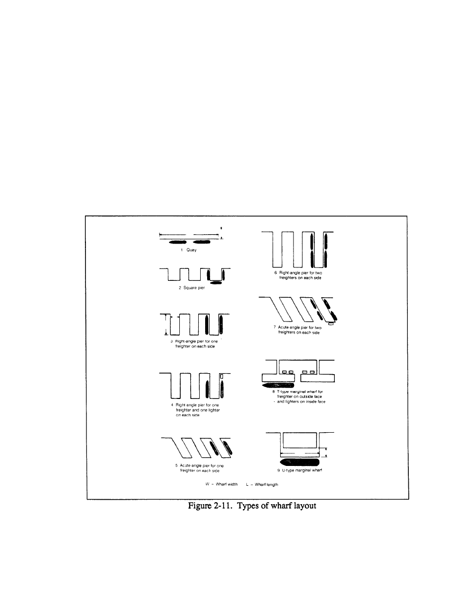
PART ONE
Terrain Evaluation and Verification
FM 5-33
An offshore pipeline berth is connected to the shore solely by a submarine or
floating pipeline, which permits cargo transfer directly to storage installations on
shore.
In a terminal buoy system, the terminal buoy looks similar to the standard mooring
buoy but is substantially larger. It is positioned offshore in deep water with three
or more chains attached to heavy anchors. The terminal buoy has a revolving
platform or swivel to which the tanker is secured as are the floating hose lines for
cargo, bunker oil, and fresh water. When the buoy’s flexible hoses are coupled to
the ship’s system, this permits ship and hose lines to swing together a full 360
degrees with the wind or sea. Product transfer proceeds through submarine
pipelines connecting the buoy and ashore installation.
Wharf construction and materials vary greatly; however, most structures are
either open or solid construction. Open construction is used for marginal wharves,
offshore wharves, and most piers. In its simplest and least permanent form, it
consists of open-spaced wooden piling supporting a wooden deck. Variations
designed to contribute to the strength and permanence of the open structures are
2-25

FM 5-33
Terrain Evaluation and Verification
PART ONE
numerous. Substructures may consist of steel or precast concrete piling. The
superstructure or decking may vary from wooden joints and flooring to concrete
and steel construction with an asphalt or other paved surface.
Solid construction is used in quays (and occasionally in piers) and consists of a
solid backfill against a retaining wall and covered with a surfaced decking. Quay
walls may be a simple facing of interlocking sheet steel pinning, a monolithic
concrete wall, or a masonry structure built of stone or precast concrete blocks.
Many quays abroad consist of large concrete caissons sunk in line to forma wall,
then filled with concrete or rubble and capped with a reinforced concrete deck.
Wharves require several basic dimensions; careful measurement and precise
identification of reference points is essential. Measurement may be in either feet
or meters, since conversion tables are available.
The length of one side of a pier may differ from that of the other, and both should
be reported. The side of a pier or the face of a wharf may be irregular or stepped,
and a dimension should be reported for each segment. Usable berthing space may
or may not coincide with the overall length; shoals or other obstructions may
decrease the usable length of a wharf.
The width of a marginal wharf may be difficult to determine, since the inner limit
may not be defined. In such cases, the measurement points should be clearly
identified. Width of apron is not to be confused with width of wharf. The apron
is the working part of the wharf deck at shipside; it terminates at the transit shed
or other obstruction.
The type and condition of the deck surface has an important bearing on the
usability of a wharf. Analysts should indicate the layout of wharf railroad tracks
with respect to the wharf deck. They should be particularly careful when reporting
berthing capabilities of a wharf. Special or unusual berthing conditions include the
breasting of ships off the wharf by means of pontoon, the presence of surge or swell
that might require special mooring precautions, and draft limitations.
Harbor Craft
The operation of most ports requires a fleet of various harbor crafts. Although in
large ports the composition of the fleet may undergo frequent changes, information
about types, general numbers, and operating characteristics of harbor craft is
essential.
Tugs are generally seagoing or harbor. Analysts should list the horsepower,
power type, operating range of seagoing salvage tugs, and special equipment such
as salvage or fire-fighting equipment. When no tugs are present, launches are
important. They may be grouped by horsepower and power type.
Lighters may be broken down by size and type (self-propelled and dumb); in large
ports their numbers may be given in round figures. Information requirements
include such details as capacity, construction, power type, and specialized lighters
for handling ammunition.
Harbor-dredging operations use dredges, hopper barges, and rock breakers.
Dredges vary in type and mechanism, depending on the nature of the bottom
2-26

PART ONE
Terrain Evaluation and Verification
FM 5-33
sediments to be worked. Hopper barges are self-propelled or dumb barges fitted
with self-emptying hoppers. They haul material recovered by dredges. Rock
breakers, as the name implies, are used in special cases when loosening of rock
from the harbor floor is required.
Shipyards
Completeup-to-date information is required on shipyard facilities and on all firms
capable of making marine repairs but lacking dry-dock facilities. Valuable infor-
mation is contained in maps, yard plans, individual facility plans, shop layouts,
photographs of yard facilities, and docking manuals. Each shipyard should be
positively identified by position within a city or port, with references to outstanding
landmarks on watefront, rivers, and tributaries.
The principal types of dry-dock facilities are the graving dock, floating dry
dock, and marine railway. The three gate types provided for graving docks are leaf
gates, flap gates, and sliding caissons. Leaf gates are hinged swinging gates that
fold back into recesses in the walls of the entrance when the dock is open. Flap
gates arc hinged at the bottom and lowered outward to a horizontal position in the
approach to the dock. The sliding caisson rolls or slides on a track on the dock sill.
Ship construction and conversion are not treated in detail in port studies dealing
with terrain intelligence; however, information about the physical facilities used in
construction and repair are valuable to the intelligence analyst. This information
includes the types of structural, engineering, electrical, and miscellaneous shops in
which various shipbuilding and ship repair processes are performed; the types of
ships constructed and the largest of each type constructed to date; whether repairs
can be made without dry docking by means of caisson; the yard’s reputation for
speed in accomplishing repair work; and the general capabilities of the yard as to
hull, engineering, and electrical repairs.
Naval Bases
Natural features required of a good naval-base site include a harbor with deep-
water approaches; protected and spacious deep-water anchorages; positions
capable of being easily defended; sufficient land for expansion; elevation of
approximately 1.5 to 3 meters above mean high water at the waterfront; suitable
ground for the foundation of dry docks, buildings, and heavy equipment; and an
ample supply of safe, freshwater. Local labor, materials, and transportation must
be adequate to support the operation. Secondary stations of the shore establishment
are necessary to fleet operation.
Although they will vary in both size and relative importance, certain functional
components are common to given types of naval bases. Submarine bases will
almost always contain a torpedo shop, battery repair shop, electrical battery-charg-
ing equipment, and high-pressure air-charging equipment. Medical components
of a large activity may contain, in addition to the normal medical and dental
equipment, specialized equipment and resuscitating gear for divers. Analysts
should indicate whether or not a particular component is included among the base
installations.
Landings
Landings may be structures that are usable for landing, although primarily
designed to serve some other function, or they may be beaches in the harbor on
2-27
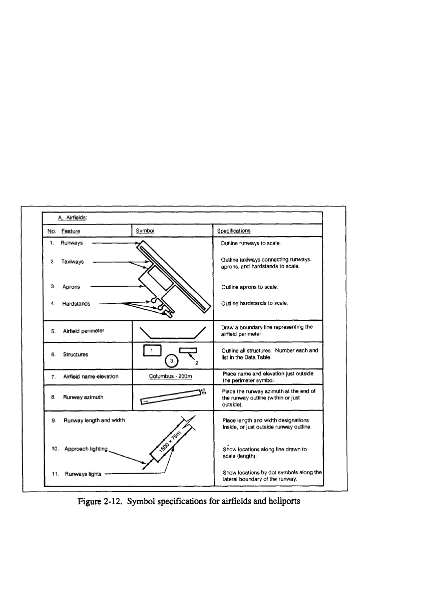
FM 5-33
Terrain Evaluation and Verification
PART ONE
which landings are possible. Landings assume particular importance when a port
becomes unusable by damaged or sunken vessels and when they must serve as the
supplemental or principal medium of transfer between ship and shore. These
structures include breakwaters, sea walls, bulkheads, seaplane ramps, and beaching
hardstands. In wall-type structures, the length, depth alongside as referred to chart
data, height of the top above chart data, and batter of face wall are significant. For
all structures, analysts should identify the construction type, condition of the sea
and current alongside, and clearance facilities.
Airfields
Air facilities are the military and civilian installations upon which a nation’s air
operations depend. The fundamental air facilities are airfields, seaplane stations,
and heliports. Each has its own facilities such as runways, hangars, fuel systems,
maintenance ships, and crash, fire, and service equipment. At some small foreign
airfields, many functions may be combined in one or two centrally located build-
ings.
2-28
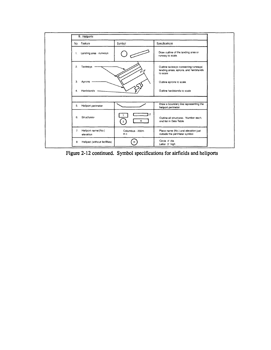
PART ONE
Terrain Evaluation and Verification
FM 5-33
The most advantageous location for an airfield is an area free from natural and
cultural impediments to operations. An elevated rather than low area is preferred
because of-the absence of terrain obstructions and generally more favorable local
weather conditions. Low areas are frequently exposed to adverse wind conditions,
fog, and occasional flooding. Another important factor in airfield location is its
intended use. Major civil airfields will almost always be located near the cities
they serve. Major military installations, which normally require more land because
of their vast complex of fixed facilities, are more often constructed some distance
away from large cities. See Figure 2-12.
Auxiliary airfields are normally located near major operational or training bases.
Often these facilities are on caretaker status during part of the year when their
additional capacity is not needed.
A helipad is an area specifically designated and marked for helicopter landings
and takeoffs. The surface of the pad may be natural, temporary, or permanent. A
helistop refers to a helipad with little or no facilities and is used for on- and
off-loading of cargo or passengers.
An airfield runway is a flat landing surface with a true or magnetic heading,
normally taking advantage of prevailing winds. The number of runways or runs
may vary from one to several, which are usually oriented in different directions.
Some airfields have parallel runways (two runways with the same headings - not
to be confused with a parallel taxiway). Runways are the most significant features
of an airfield, and detailed information concerning them, taxiways, and parking
areas is essential to properly evaluate the airfield’s capabilities. The length, width,
2-29

FM 5-33
Terrain Evaluation and Verification
PART ONE
load-bearing capabilities, and pavement condition directly influence the type and
amount of traffic an airfield can accommodate.
Taxiways are access paths to parking aprons, hangar aprons, and handstands or
revetments. A parallel taxiway parallels the runway but is usually narrower. Under
emergency conditions it may be used as a runway, but it should not be reported as
a runway. Link taxiways connect the runways with other taxiways, parking and
hangar aprons, or revetments. A perimeter taxiway usually starts at one end of the
runway and ends at the other, and is normally oval. Loop taxiways are normally
located at or on both ends of the runway, forming a loop. The alert taxiway is
located at the end of the runway with clear access to the runway for a scramble by
fighter interceptors.
Runways, taxiways, aprons, and revetment surfaces may be permanent, tem-
porary, or natural. Permanent surfaces such as concrete or asphalt have distinct
edges and ends, while temporary surfaces such as mixed-in-place madam or oiled
earth have ragged and uneven edges and ends. Permanently surfaced runways are
easily discernible and may have jet barriers or arrester gear. Jet barriers are located
on the overrun, whereas the arrester gear is normally flush with the runway and
located approximately 500 meters from the end of the runway. This 500 meters is
usable runway and should not be confused with an overrun.
Measuring permanent or temporary surfaced runways should not be difficult. The
major difficulties are locating and arriving at the measurements of natural surface
marked with painted barrels, reeks, or broken white lines. Runway lengths and
surfaces vary according to the use or intended use of the airfield.
The weight- or load-bearing capacity of a runway, taxiway, or apron is a
determining factor in its capability to accept aircraft without damage to the aircraft
or the facility. The engineering factors involved in determining weight-bearing
capacity are complicated; however, other sources for this information are route
manuals, air information publications, airfield managers, and engineering docu-
ments. If these sources are not available, information about the type and weight of
aircraft (partially or fully loaded) operating out of a given airfield will enable the
analyst to estimate the weight-bearing capacity of the runway.
2-30

PART TWO
Analysis Procedures
FM 5-33
Natural Terrain
Chapter 3
SURFACE-CONFIGURATION OVERLAY
The surface-configuration overlay is used to depict the inclined surface of the
terrain and is expressed using percent of slope or change of elevation (rise) divided
by the horizontal distance (run).
This overlay is one of the primary overlays used in determining the cross-country
movement capability of troops and vehicles.
A 1:50,000 topographic map is required to construct a surface-configuration
overlay using TTADB product specifications.
Step 1.
Examine topographic maps. Construct a surface-configuration overlay
for the TTADB using a standard 1:50,000 topographic map with a variety of
possible contour intervals. A contour interval of 20 feet or less is preferred for
constructing this overlay.
Register the overlay to the database or map you are using. Cover the selected
topographic map with a clean sheet of mylar and tape them together. If the area of
interest does not cover the entire map, outline the area of interest on the mylar in
black pencil or ink and note the longitude and latitude or UTM coordinates at the
corners.
Annotate the map sheet name and number, map series, map edition, scale, contour
interval, factor overlay type (surface configuration) and classification, if required,
on the overlay.
Step 2.
Depict surface-drainage features. Trace the boundaries, in black pencil or
ink, of all islands longer and wider than 250 meters (5 millimeters at the scale of
1:50,000). Show long, narrow islands (those less than 250 meters wide) only if
they are greater than or equal to 1000 meters in length (20 millimeters on the map).
Trace the boundaries of all open-water bodies such as ponds, lakes, reservoirs,
and double-lined streams in black pencil or ink. Label all open water with a W.
3-1
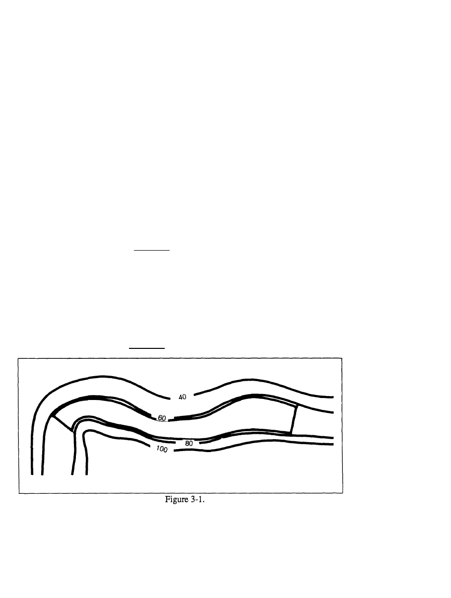
FM 5-33
Analysis Procedures
PART TWO
Step 3.
Depict dissected terrain. Trace the boundaries of all naturally and/or
culturally dissected land areas in black pencil or ink and label with a G. Dissected
terrain includes, but is not limited to, pits, quarries, dumps, landfills, piles, ravines,
and gorges. Many of these features are easily recognized on topographic maps.
Step 4.
Outline and label slope categories. Select a slope calculator (See Figure
3-1.) that was constructed for the scale and contour interval of the map used A
slope calculator, also called a template or wedge, is an instrument for measuring
the percent of slope on a topographic map. This instrument is constructed of a
transparent, stable-base material and is marked with predetermined distances that
correspond to the desired slope category. Ensure the slope calculator has the
required slope categories established within the TTADB product specifications. If
a suitable slope calculator is not available, you must construct one for the map you
are using.
Example: Construct a slope calculator for slope categories of 0-3 percent and
3-10 percent, given a 1:50,000 topographic map with a contour interval of 20
meters.
a. Determine the horizontal distance required, with an elevation difference
(contour interval) of 20 meters to equal the largest slope percent of a given category.
HD = CI x (100)
% slope
HD = horizontal distance
CI = contour interval
% slope = largest slope percent of a given category
(100) = constant
Formula: Slope category A (O to 3%)
HD= 20 x (100)
3
3-2

PART TWO
Analysis Procedures
Hd = 666.6 meters (CI was in meters)
Formula: Slope category B (3 to 10%)
FM 5-33
HD = 20 x (l00)
10
HD =200 meters
b. Determine the map distance, or the spacing of the contour intervals, required
to construct the slope calculator for categories A and B:
MD = map distance
HD = horizontal distance (from previous formula)
D = denominator of map scale
Slope Category A (0-3%)
MD = .01333 meters or (13.33 mm)
Slope Category B (3-10%)
MD = .004 meters or (4 mm)
Note: You must calculate map distances for each slope category outlined in TTADB product
specification (PS/3JB/020) and for any slope category required for a special-purpose product.
c. Construct the slope calculator. Construct the slope calculator using the map
distance calculated from the above formulas on a clear, stable-based material.
Draw several ticks representing the same slope category.
d. Outline the slope categories. Analyze the contour lines on a topographic map
using the slope calculator to outline and label slope categories. Slope categories
are areas on a map where the slope is the same or is in the same category.
Start the slope analysis in the upper left-hand comer of the map and determine
map areas whose slope (contour interval) matches the O to 3 percent (or lowest
category required) slope category on the calculator (See Figure 3-2). When you
have outlined all areas within this category using a black pencil or ink, label all
outlined areas with an A or representative symbol from your legend.
Continue this analysis for all slope categories that you have outlined and labeled.
Prepare the surface-configuration legend according to TTADB product specifica-
tions.
3-3
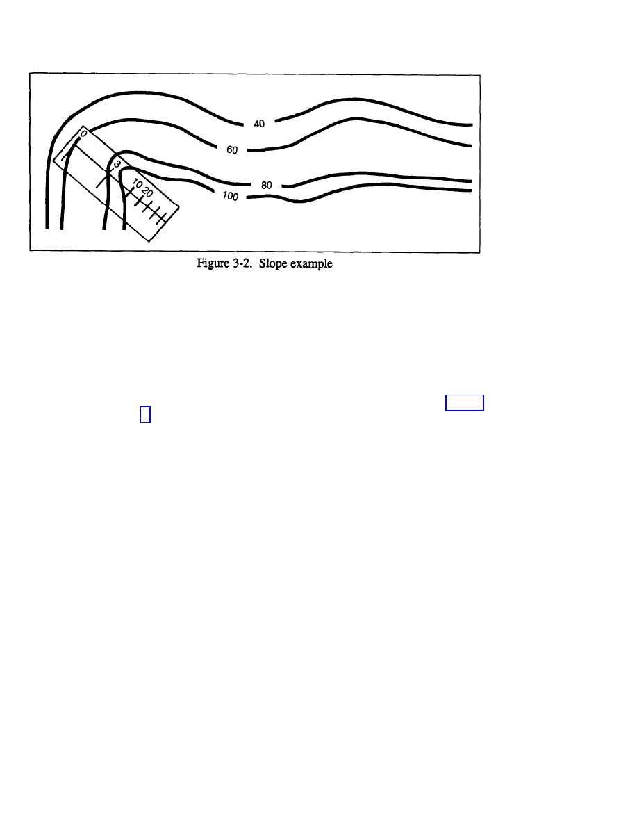
FM 5-33
Analysis Procedures
PART TWO
Step 5.
Determine slope from aerial photography. Determining slope from aerial
photography requires complete stereo coverage. It is time-consuming and requires
more skill than using a topographic map. You should use this method only if
topographic maps are not available or if you need precise slope measurements from
a point to a point. You cannot use this process to compile a surface-configuration
factor overlay, since this overlay is keyed to a topographic base map.
Step 6.
Construct the final overlay. The final step in producing a factor overlay
is to put the draft manuscript overlay into a final database product. You must have
support from the cartographic and reproduction elements or sections. See Chapter
8 for the final overlay procedure.
VEGETATION OVERLAY
The vegetation overlay shows natural and cultivated vegetated areas, with infor-
mation about type, size, and density. This factor overlay is one of the primary
overlays used in determining the cross-country movement capability of troops and
equipment, cover and concealment line of sight, and location of construction
resources.
A 1:50,000 topographic map and complete stereo imagery is required to construct
a vegetation factor overlay using TTADB product specifications.
Step 1.
Collect required collateral data. The vegetation factor overlay is one of
the most complex and difficult factor overlays terrain analysts construct. No single
source data can provide all of the data required to complete the vegetation factor
overlay and data tables. In most cases, analysts must use different sources for
different geographic areas. Unlike other factor overlays, where terrain factors are
similar worldwide, geographical location, climate, soils, and the agricultural prac-
tices of the location being analyzed greatly influence the vegetation factors. Some
of the major sources are maps, literature, and aerial imagery.
Military topographic maps. Standard military topographic maps differ in com-
pleteness according to scale and country of origin. The boundaries of forested areas
3-4
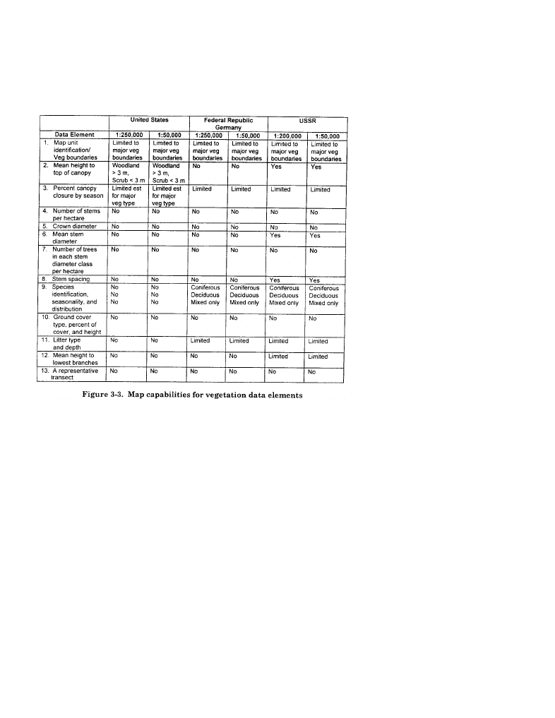
PART TWO
Analysis Procedures
FM 5-33
are generally accurate on topographic maps but size, type, and density information
cannot be obtained from the map alone. See Figure 3-3.
Small-scale vegetation maps. This product can be found in any general geography
text and usually depicts very broad categories of vegetation. It does not give
enough of the detailed information required but will give analysts background on
agricultural practices and the predominant vegetation types of the area.
Species distribution maps. These maps are produced under a variety of names
depending on their geographical location and the type of data they present. They
are produced primarily for use as forestry tools by government agencies, commer-
cial lumber companies, and colleges and universities. They provide extremely
detailed information but are produced for limited areas and specific functions. If
they are not available, the analyst should query local government agencies and
universities located in the area of interest. This is only feasible if the area of interest
is accessible to the terrain analyst and if local agencies are friendly and willing to
a
SS
i
S
t.
Literature. Literature is nearly unlimited in quantity, scope of subject matter, end
coverage of geographic regions. Data from this source is usually too general to be
of much use but can be used to verify other data.
Aerial imagery. Analysis of aerial imagery is the best and most accurate method
of obtaining detailed vegetation information. The quality of information obtained
depends largely on the skill and knowledge of the individual analyst and the type
and quality of the imagery available.
Step 2.
Determine data elements. After identifying and collecting sources of
information, analysts must determine the data elements or essotial elements of
3-5

FM 5-33
Analysis Procedures
PART TWO
terrain information (EETI) required to produce the vegetation factor overlay. The
data elements required are--
Vegetation-area boundaries.
Vegetation type.
Height to top of canopy.
Canopy closure.
Sterns per hectare.
Stem diameter.
Stem spacing.
Ground cover.
Height to lowest branches.
Seasonal information.
Step 3.
Prepare collateral data. Gather all available data that covers the area of
interest. Examine the information to ensure completeness and accuracy, to see if
some of the information is old or dated, and to see if newer sources are available,
Vegetation can be influenced by man’s activities and can change in a relatively
short period of time.
Identify information gaps. After all available information has been gathered,
superimpose it on the base map to determine areas where information does not
exist or is too old to be reliable.
Submit collection requirement. If information gaps exist, determine alternate
available sources and submit the appropriate collection requirement. The collec-
tion request can be for new imagery or for on-site verification of dated information.
Step 4.
Prepare topographic map base. Construct the vegetation overlay for the
TTADB using a standard 1:50,000 topographic map. Register the overlay to the
data base or map you are using. Cover the selected topographic map will a clean
sheet of mylar and tape them together. If the area of interest does not cover the
entire map, outline the area of interest on the mylar in black pencil or ink and note
the longitude and latitude or UTM coordinates at the corners. Annotate the map
sheet name and number, map series, map edition, state, factor overlay type
(vegetation) and classification, if required, on the overlay.
Prepare the data table worksheets. Trace the boundaries, in black pencil or ink,
of all open-water bodies such as ponds, lakes and double-lined streams and label
them with a W.
Trace the boundaries of all built-up areas that are longer and wider than 250
meters (5 milimeters at 1:50,000 scale). Label the outlined areas with an X.
Step 5.
Determine vegetation types and boundaries. Trace the boundaries of all
forested areas. For the working overlay, label all forested areas with a T. Further
analysis will determine type, size, density, and internal boundaries or changes.
Trace the boundaries of all agricultural areas and label the areas with an A.
Determine the type of crops, such as dry, wet, terraced or rotating/shifting crops
and add the second agricultural code (see Figure 3-4,). The analysis of collateral
data will be required to determine the second code.
3-6
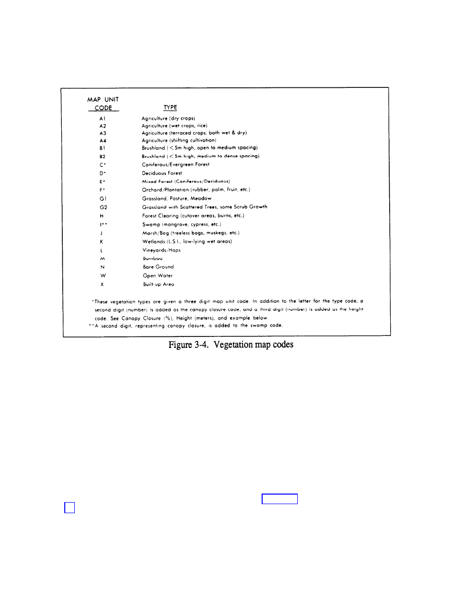
PART TWO
Analysis Procedures
FM 5-33
Trace the boundaries of all brushlands and label them with a B1 or B2, depending
on the vegetation category. The analysis of collateral data will be required to
determine the second code.
Trace the boundaries of all grasslands and label them with a G1 or G2, depending
on the vegetation category. The analysis of collateral data will be required to
determine the second code.
Trace the boundaries of all swamps (I), marshes and bogs (J), and wetlands (K)
and label them accordingly.
Step 6.
Determine forest type and boundaries. Since different types of trees have
different characteristics and have a major impact on cross-country mobility, on
cover and concealment, and on use as engineering resources, you must determine
the forest type and the transition boundary of the areas already labeled T.
Trace the boundary of all coniferous/evergreen forests and label them with a C.
This forest category must contain 60 percent or more species of coniferous trees.
These trees are relatively easy to place within a broad classification because they
tend to have definite sizes and shapes. Shadows, crown shape (see Figures 3-5 and
3-6) and photographic tone are the most common photo interpretation keys.
3-7
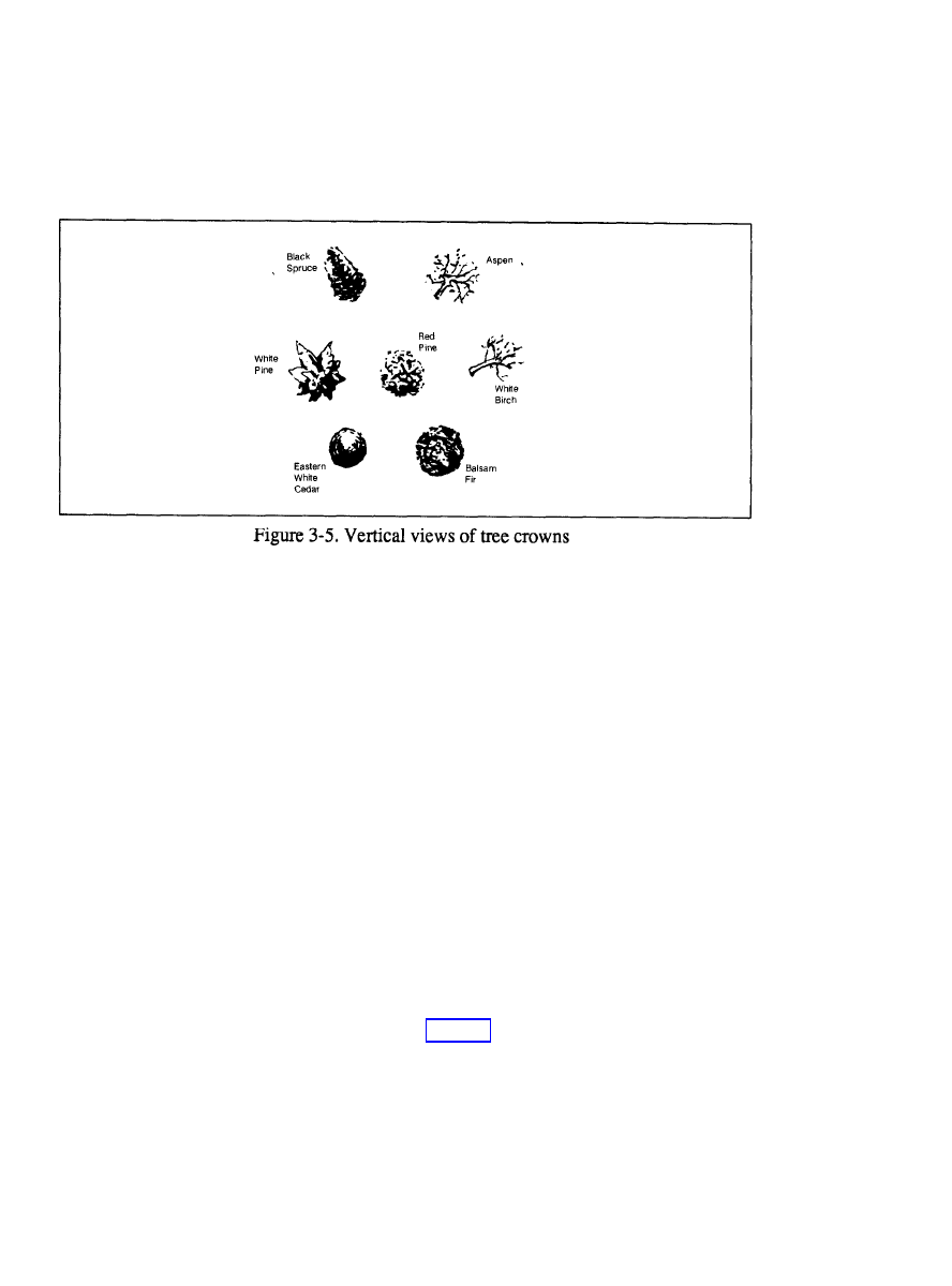
FM 5-33
Analysis Procedures
PART TWO
Trace the boundaries of all deciduous forests and label them with a D. This forest
category must contain 60 percent or more species of deciduous trees.
Trace the boundaries of all mixed forests and label them with an E. Mixed forests
are those forests that do not contain 60 percent or more of either coniferous or
deciduous trees.
Trace the boundaries of all orchards and/or plantations and label them with a F.
This category can be identified by the uniform rows and photographic tone and
texture. Analysis of the collateral data will key analysts to look for this vegetation
type and location.
Step 7.
Determine canopy closure. Canopy closure is the percent of ground area
covered by the tree crown and is normally computed only for forested areas. Crown
area is the area covered by the vertical projection of a tree crown to the horizontal
plane.
Vegetation types indicated by C, D, E and F are given two digits in addition to
the letter. The letter denotes the tree type, the first number represents the canopy
closure, and the second number is the&e height. For swamps (I), the third digit
or height code is omitted.
Canopy closure is coded in four categories:
CODE
CANOPY CLOSURE %
1
0 - 25
2
25 - 50
3
50 - 75
4
75 - 100
Use the crown density scale to determine the canopy closure. It is made of
columns of squares containing solid black circles. These circles cover and repre-
sent a percent of the area (see Figure 3-7 within the square). Match the appropriate
scale to the forested area on the imagery and record the crown density for a given
area.
3-8
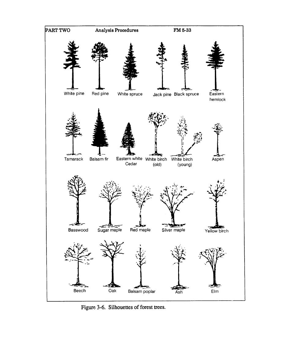
Note: When tree shadows
fall on level ground, they often
Compare only the tree crown and not the shadows visible on the photo. Factors
permit identification of in-
affecting accuracy of canopy closure measurements include--
dividual species.
3-9
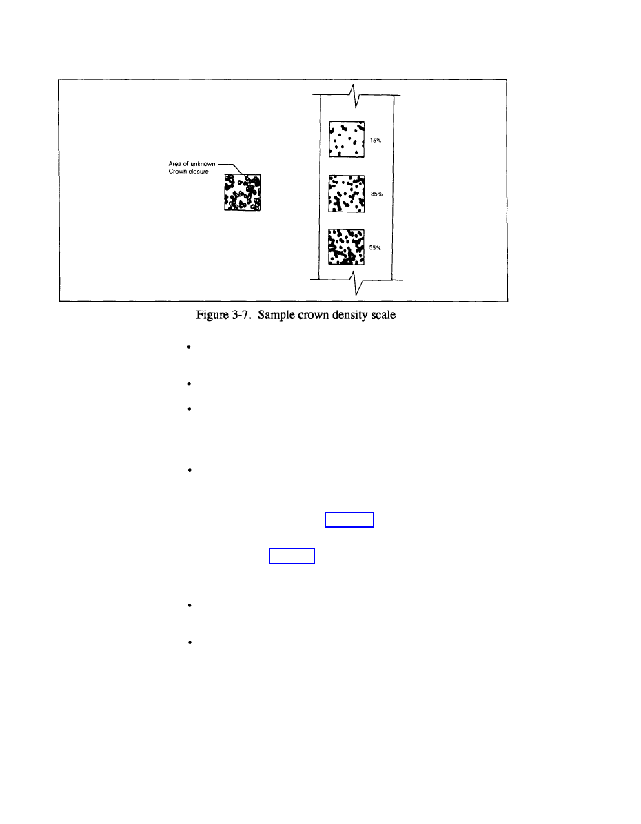
FM 5-33
Analysis Procedures
PART TWO
Image quality. Crown closure estimates of forest stands on poor quality
photographs tend to be too high because of the lack of detail in photo
tones and the inability of the analyst to identify small crown openings.
Shadows. Shadows tend to mask stand openings causing the stand to ap-
pear more dense.
Photographic scale. The minimum canopy opening that can be identified
on photography is directy related to the photographic scale. Small open-
ings which can be identified on 1:6000 scale photography cannot be seen
on 1:20,000 scale photography. The net effect is to overestimate canopy
closure when using small-scale photography.
Analyst skill. An average analyst using good quality photography should
produce crown closure estimates accurately to within 10 percent.
Step 8.
Determine the mean height to top of canopy. The second number, or
third digit, depicts the tree height (see Figure 3-8). Mean height to top of canopy
is the mean or average height of a specific tree type or category. If existing data
to determine and outline mean tree height does not exist, use aerial photography to
measure tree height (see Chapter 9). Three methods to measure tree height from
aerial photography are the parallax, shadow, and relief displacement methods.
Factors affecting the accuracy of height measurements include--
Photographic scale. Tree height measurement error generally increases
when small-scale photography is used due to the inability of the analyst to
identify the tree’s apex.
Character of forest. Measurement of tree height is dependent on the
analyst’s ability to seethe ground nearby. This is closely related to the
stand density and ground clearance. If a forest stand is very dense, such
as a tropical rain forest, it is very difficult to find an opening large enough
to permit accurate measurements.
3-10
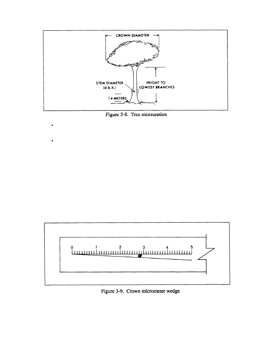
PART TWO
Analysis Procedures
FM 5-33
Terrain relief. Trees growing in areas that are not level are difficult to
measure accurately because of a tendency to refer measurements to
canopy openings at elevations different than those at the base of the tree.
Analyst skill. An analyst should be able to determine the height of trees
accurately within each map unit. Knowledge of forest conditions and clas-
sification of specific tree type (species) can be an invaluable aid in height
classification.
Step 9.
Determine tree crown diameter. Tree crown diameter is the distance
across the spread of a tree crown and is measured in meters. Diameter measure-
ments of the largest, average, and smallest crowns in each category will determine
the average crown diameter for a given map unit. This measurement is made using
the dot-type scale or the crown micrometer wedge on the photograph (see Figure
3-9).
Select a tree for measurement. Slide the dot-type scale alongside the tree until
you find a dot that is equal in size to the tree’s crown. It is best not to fit the circle
over the crown, because too much detail is screened by the black dot or circle.
3-11

FM 5-33
Analysis Procedures
PART TWO
Select a tree for measurement. Place the micrometer wedge so the insides of the
two diverging lines are just tangent (making contact at a single point) to the tree.
Take a reading at the point on the scale where the tree crown is tangent to the
diverging lines.
Take an average of three measurements using either method. The answer will be
in millimeters of photo distance. Convert the answer to ground distance by
multiplying by the denominator of the photo scale. Convert millimeters of ground
distance to meters by dividing by 1000. Factors affecting accuracy of crown
diameter measurement include--
Photographic scale. The analyst’s ability to accurately identify the
largest, average and smallest crowns is closely associated with the
photographic scale. Small-diameter crowns cannot be detected on small-
scale photographs, and clumps of closely spaced trees tend to be
measured as a single crown rather than as several small ones.
Location on the photograph. Limit tree crown measurements to the cen-
ter portion of the photograph whenever possible, because the center is less
affected by distortion.
Forest density. Crown diameter measurements are most accurate in open-
grown stands. Measurements in dense stands are usually limited to crown
widths for dominant trees.
Step 10.
Determine mean stem diameter. Tree stem diameter is the diameter of
a tree at 1.4 meters (4.5 feet) above the ground. This measurement is also referred
to as diameter at breast height (DBH). Calculate mean stem diameter for all
vegetation units with trees 2 meters or greater in height. Record this information
on the vegetation data table in centimeters.
Tree stem diameter is calculated using the mean crown diameter information
obtained in step 9. If this step has not been completed, calculate the mean crown
diameter for the vegetation within each map category.
When computing the stem diameter for coniferous trees, use the following
formula:
DBH (inches)= D (feet) + 5
2
Where--
DBH (inches) = Diameter at breast height
D (feet) = Crown diameter
Example: In step 9, you have determined that a stand of coniferous trees has a
mean crown diameter of 6.4 meters.
a. Convert mean crown diameter measurement to feet.
6.4 meters x 3.231 feet per meter = 20.998 feet
(Round to 21 feet)
3-12

PART TWO
Analysis Procedures
b.
c.
d.
Use the above formula to determine DBH (inches).
DBH = 21 feet + 5 DBH = 15.5 inches
2
Convert DBH (inches) to centimeters.
15.5 inches x 2.54 inches per cm = 39.37 cm
Record the mean stem diameter in the vegetation table.
FM 5-33
When computing the stem diameter for decidous trees, use the following
formula:
DBH (inches) = .75 x D (feet)
Example: In step 9, you have determined that a stand of deciduous trees has a
mean crown diameter of 8.5 meters.
a. Convert mean crown diameter measurement to feet.
8.5 meters x 3.281 feet per meter = 27.885 feet
(Round to 27.9 feet)
b. Use the above formula to determine DBH (inches).
DBH = .75 X 27.9
DBH = 20.925 inches
c. Convert DBH (inches) to centimeters.
20.925 inches x 2.54 inches per cm = 53.1495 cm
Round the answer to 53.15 cm.
d. Record the mean stem diameter in the vegetation table (see Figure 3-10)
Step 11.
Determine stem spacing. Stem spacing is the distance from the center
of one tree to the center of the nearest adjacent tree. The easiest and fastest method
to determine stem spacing is to measure directly from the photograph and convert
it to ground distance (in meters).
Use the microcomparator to measure from the center of a tree stem to the center
of the closest tree stem. This measurement unit depends on the scale used in the
microcomparator, usually made in feet, and should be converted to meters.
If the scale is not acceptable and the distance is not measurable, use the following
formula:
SS (meters )=
12.372
N
3-13
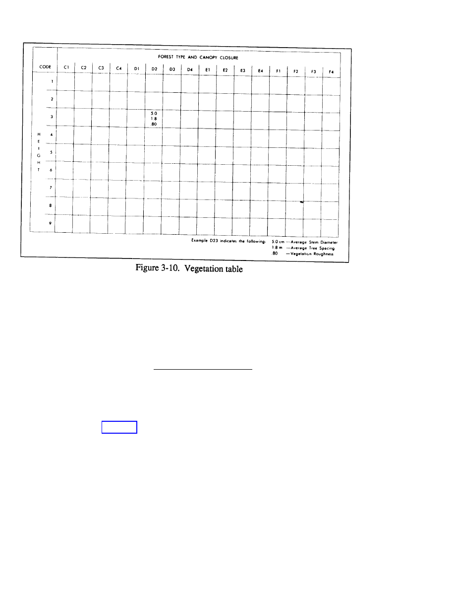
FM 5-33
Analysis Procedures
PART TWO
Where--
SS (meters) = Stem Spacing in meters
12,372 = Constant
N = Number of trees per hectare
Before you can use this formula, you must determine N. To determine N, use the
following formula:
N =
0.08
N = Number of trees per hectare
TC = Tree count in hectare scale
Determine TC (tree count in hectare scale) of a specific vegetation map code.
Orient the stereopair for viewing. Place the transparent 0.08 hectare scale (see
Figure 3-11) over the area using the appropriate photographic scale and count the
number of trees enclosed within the circle of the hectare scale.
Convert the number of trees in a 0.08 hectare to the number of trees per hectare.
Example: 32 trees were counted within the 0.08 hectare circle using the 0.08
hectare circle template.
a. Use the above formula to determine N.
3-14
TC (tree count in hectare scale)
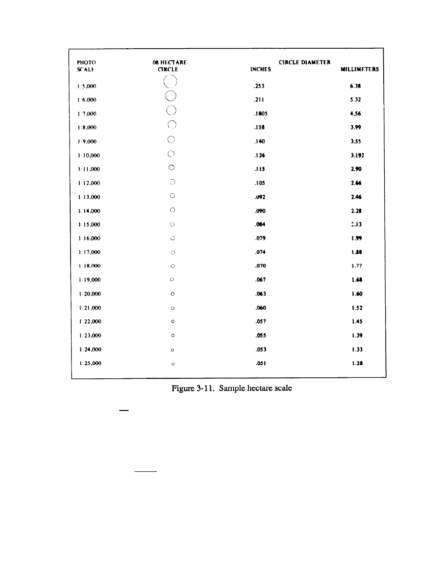
PART TWO
Analysis Procedures
FM 5-33
N = 32
0.08
N = 400
b. Use the above formula to determine SS, N = 400
SS =
12.372
400
SS = 5.56 meters
3-15
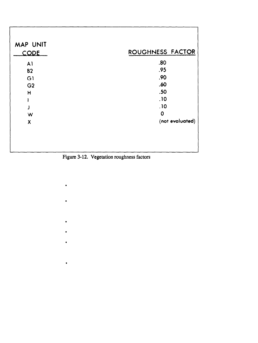
FM 5-33
Analysis Procedures
PART TWO
c. Round off to the nearest 0.1 meter and record this figure in the appropriate
column of the vegetation data table. Factors affecting accuracy of stem spacing
measurement include--
Tree spacing. Count only those trees that are visible from above and are
sufficiently large in their exposed portion to be resolved. This problem is
especially acute in tropical areas having more than one canopy.
Photographic scale. Trees with a crown diameter of less than 0.6 meters
will not be resolved at 1:12,000 scale photography. This minimum-
resolved diameter increases to 1.2 meters on photo of 1:16,000 scale or
smaller.
Tree crown diameter. Tree count accuracy increases with an increase in
tree crown diameter.
Crown canopy structure. Irregularities in crown canopy tend to increase
accuracy due to relief among trees.
Terrain. If the terrain viewed in the photograph is not level, alter the ares
represented by a given circle or adjust the crown count to obtain the true
number of trees per hectare. Compute compensation for terrain relief for
every 200-foot difference in elevation.
Analyst’s skill. Inexperienced analysts may undercount the actual mem-
ber of tree crowns by as much as 50 percent. For this reason, you must be
careful to recognize double trees, sprout clumps, or multiple groups of
trees. You can usually accomplish this by recognizing abnormally large
crowns or irregularly shaped groups of crowns.
3-16

PART TWO
Analysis Procedures
FM 5-33
Step 12.
Estimate vegetation roughness factor (VRF). The vegetation roughness
factor is an estimated numerical factor that reflects the degree of vehicular speed
degradation due to travel through a particular vegetation type on horizontal ground.
The factor decreases from 1.0 (no speed degradation) to 0.00 (vegetation roughness
does not permit off-road mobility) (see Figure 3-12). For example, grassland with
little slowdown effect would have a VRF of 1.0 to 0.9. but a virtually impassable
swamp with dense ground vegetation, fallen branches and trees, and exposed
stumps would have a VRF of .1. The factor designated to a vegetation category is
subjective and designated by the analyst. The plant’s density, stem diameter.
branching characteristics, root emergence, and so forth are all considered.
Step 13.
Prepare the vegetation legend. Prepare the vegetation factor overlay
legend according to DMA product specifications.
Step 14.
Construct the final overlay. The final step in producing a factor overlay
is to put the draft manuscript overlay into a final data base product, Support from
the cartographic and reproduction elements/sections is required. See Chapter 8 for
the final overlay procedure.
SURFACE MATERIALS ANALYSIS (SOILS)
Military planners rely heavily on soil analysis because soils vary in their ability
to bear weight and withstand vehicle passes, as well as in their ease of digging.
The moisture content and type of soil will affect road construction. material
location, and trafficability determination. The soil factor overlay breaks down the
soil types, characteristics, and distribution. Soils of the same type and quality will
have similiar strength and characteristics regardless of geographic location. The
primary factors influencing like soil strengths are environmental changes.
Describing and classifying soil normally requires extensive field sampling and
the expertise of soil scientists. The terrain analyst must be able to produce
acceptable soil factor overlays by extracting information from maps, other factor
overlays, aerial photographs, lab reports, boring logs, and other literature. The
reliability of the soil factor overlay produced will vary with the type and reliability
of the information sources. Seldom will a single source provide all of the informa-
tion required.
Step 1.
Collect required collateral data. Collect and analyze as many of the
following sources as possible for the area of interest: maps; factor overlays; special
reports, such as laboratory soil analysis reports, soil field test reports, and boring
logs and well logs; literature; and aerial photographs.
The desirable scale for all source maps is 1:50,000. If 1:50,000 scale maps are
not available, other existing maps should be converted to this scale.
Soil maps are produced by various organizations for specific purposes. Engineer-
ing firms may produce soil maps to support any type of construction project.
Government agencies may produce soil maps for agricultural purposes, land-use
planning, or special studies. The classification systems used on soil maps will vary
with the producing agency and the purpose of the map. The systems must be
translated into the USCS, which is the system used by the military for producing
soil factor overlays. See Figure 3-13.
3-17
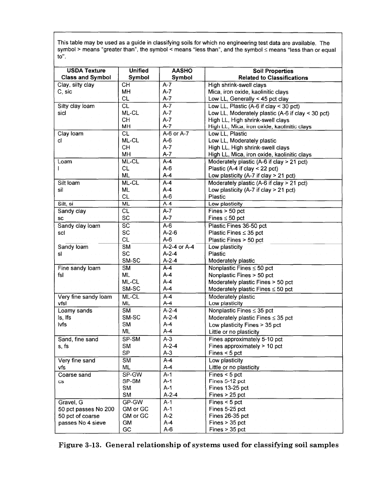
PART TWO
Analysis Procedures
FM 5-33
3-18
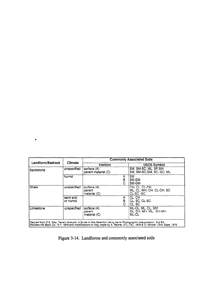
PART TWO
Analysis Procedures
FM 5-33
Some vegetation features symbolized on topographic maps can provide clues to
soil characteristics. Contours and land-use patterns can help define landforms and
identify soil types. See Figure 3-14.
Geological maps may or may not be useful form soil analysis. Those maps which
show the surface profile to bedrock usually define the type and depth of soil, as
well as the parent material or bedrock.
In some cases, vegetation (or change of vegetation) can be an indicator of a
specific soil type, change of soil type, or change of soil depth.
Climatic maps provide annual variations in temperature and moisture conditions.
Of particular interest is information concerning the state of ground; for example,
wet, dry, moist or frozen. This information is important in determining the stability
of a soil or changes of stability with seasonal changes.
Literature reports are published by academic institutions, government agencies,
or private firms on soil-related subjects such as soil, topography, geology, and
vegetation.
Analysis of air photographs is the best overall method for obtaining soil informa-
tion for large and inaccessible areas.
Step 2.
Determine data elements. Once you have identified and collected the
sources of information, determine the data elements, or EETI, required to produce
the soils factor overlay. The data elements required are--
The soil profile, which is a description of the soil with depth, including
identification of soil layers; depth ranges for each horizon layer in
3-19
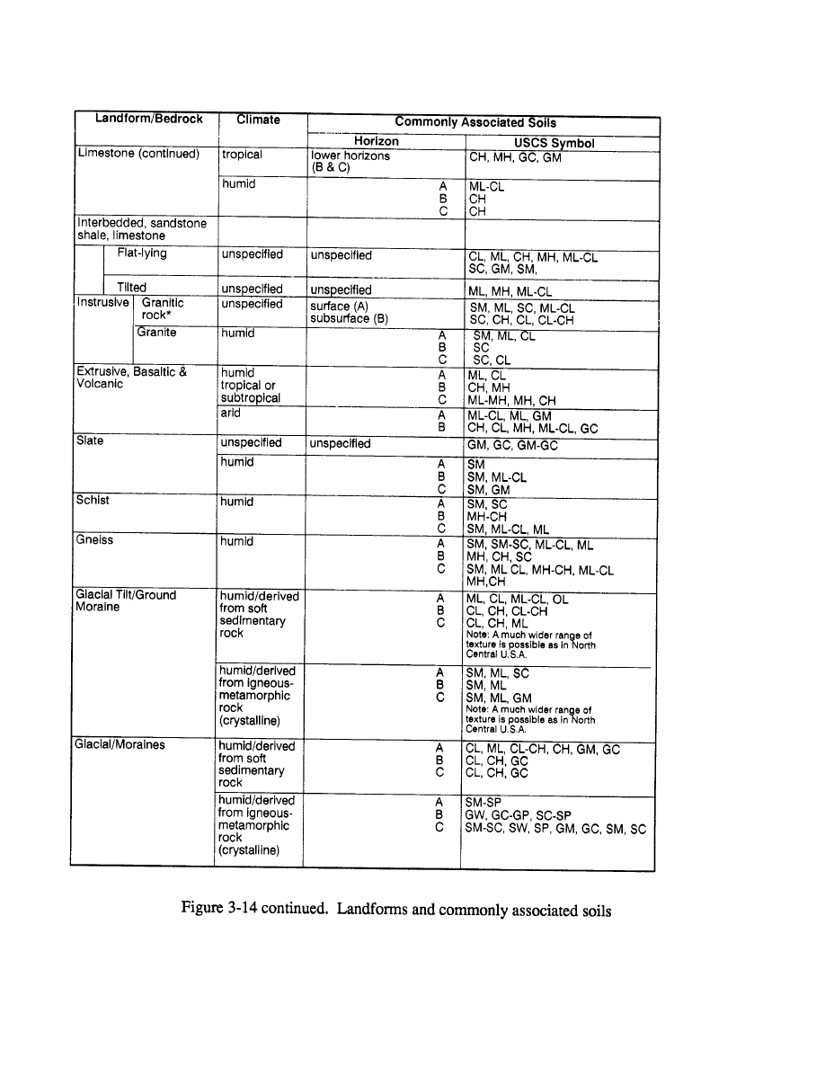
FM 5-33
Analysis Procedures
PART TWO
3-20
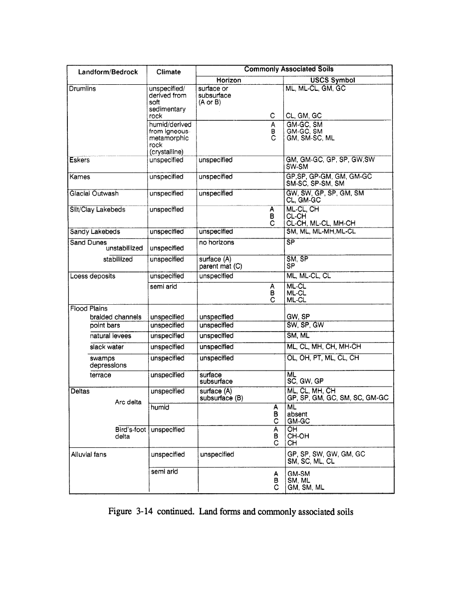
PART TWO
Analysis Procedures
FM 5-33
3-21
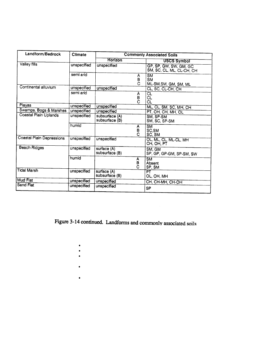
FM 5-33
Analysis Procedures
PART TWO
Note: *Granitic rock includes
rhyolite porphyry, trachyte por-
phyry, dacite porphyry, basalt
meters; and identification of soil type for each horizon with one of the 15
porphyry, augitite porphyry,
USCS symbols.
granite, syenite porphyry,
Depth to bedrock, or the total thickness of soil in meters.
syenite,
diorite
porphyry,
diorite, gabbro porphyry, gab-
State-of-ground, or the average monthly moisture condition of the soil.
bro,
pyroxenite porphyry,
Stoniness, or the estimated number of stones of a given diameter per
pyroxentie periodotite
volume of soil, which may be expressed as a percentage of the volume.
The rating cone index (RCI), an on-site or estimated value of soil
strength derived from the cone index multiplied by the remolding index.
The cone index (CI), the field measurement indicating the shearing resis-
tance of soil, obtained with a cone penetrometer.
3-22

PART TWO
Analysis Procedures
FM 5-33
The remolding index (RI), a ratio that expresses the proportion of original
strength that will be retained by a fine-grained soil or a sand with fines,
poorly drained, after being subjected to vehicular traffic.
Step 3.
Prepare collateral data. Gather all available soil maps that cover the area
of interest. Examine their scales and legends. Extract those at 1:50,000 scale or
larger that use the USCS. If any of these maps are based on field surveys (field
classification), they may be used as the soil factor overlay base. Further data
analysis or extraction may be unnecessary if the soil maps can produce all the
information required by the data elements.
Step 4.
Prepare topographic map base. Extract the topographic maps that cover
the area of interest. A scale of 1:50,000 with a contour interval of 20 feet or more
is preferred.
Cover the selected topographic map with a clean sheet of mylar and tape them
together. If the area of interest does not cover the entire map area, outline the area
of interest on the mylar in black pencil or ink and note the longitude and latitude
or UTM coordinates at the comers. Register the overlay to the data base or map
you are using.
Annotate the map sheet name and number, map series, map edition, scale, factor
overlay type (surface materials) and classification, if required, on the overlay.
Trace the boundaries of all open-water bodies such as lakes, ponds, and double-
line streams in black pencil or ink, and label them with a W.
Trace the boundaries of all built-up areas that are longer than 250 meters (5
millimeters at 1:50,000 scale). Label the outlined areas with an X.
Trace the boundaries of all permanent snowfields in black pencil or ink, and label
with a them PS.
Trace the boundaries of all areas of salt evaporators and salt encrustation in black
pencil or ink, and label them with an EV.
Step 5.
Determine soil types and boundaries. Evaluate collateral source material
for soil boundaries and types. If data does not already exist, analyze landforms,
vegetation, and geology information to determine USCS type and boundary.
Trace the boundaries of all areas of exposed bedrock or void of surface soils in
black pencil or ink, and label them with an RK.
Evaluate the soil factors and place appropriate boundaries on the overlay in black
pencil or ink, using the topographic map as a base.
Label all evaluated areas with the appropriate USCS symbol. If information
conflicts exist between different source materials, use the most reliable and current
information available. Assign to each different area (soil type) a map unit number,
numbering from top to bottom and left to right. Areas with the same surface soil
type and identical horizon information will have the same map unit number. Do
not assign map unit numbers to RK, PS, EV, X and W areas. The third digit after
the USCS symbol shows the surface roughness factor.
3-23
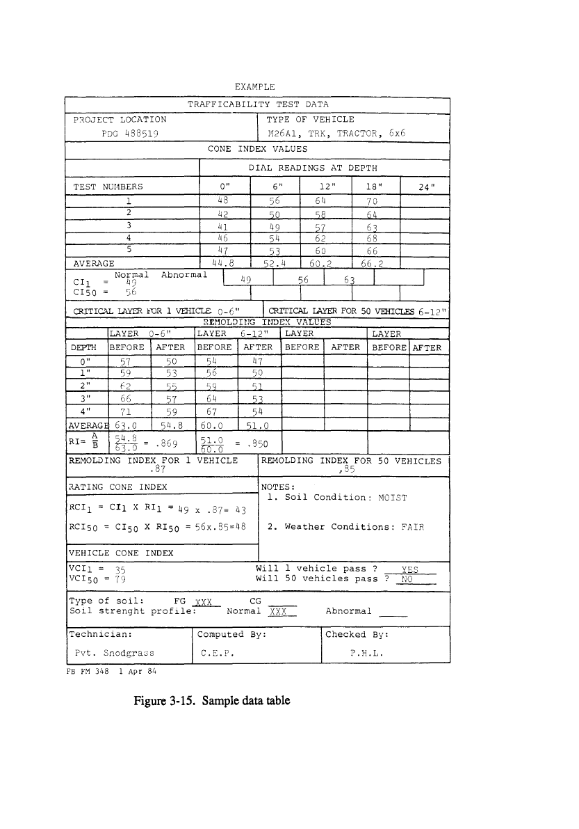
FM 5-33
Analysis Procedures
PART TWO
3-24

PART TWO
Analysis Procedures
FM 5-33
Step 6.
Determine surface roughness. Surface roughness factors are estimated
factors used to compute the degree of degradation of the rate of vehicle movement
caused by surface characteristics. These factors are tailored for each job by listing
only those features encountered. Surface roughness is that aspect of the surface
materials (such as boulder fields, gullies, and rugged bedrock.) which reduces
vehicle speed.
Factors can be any number from 0.00 to 1.00 in 0.05 increments. The surface
roughness factor of 1.00 for a vehicle class would indicate no degradation while a
0.80 factor would degrade vehicle speed by 20 percent. In estimating the mag-
nitude of the factor, consider all physical characteristics of the feature as well as
vehicle characteristics such as ground clearance and wheel size.
Surface roughness is classified for five types of movement categories: medium
and large tanks, large wheeled vehicles, small wheeled vehicles, small tracked
vehicles, and foot troops. Surface roughness factors often vary from one vehicle
class to another.
Step 7.
Prepare surface materials legend. Prepare a soil data table with RCI
values for wet and dry seasons (see Figure 3-15). Using all available information,
annotate the data elements required to complete the soil data table. This informa-
tion can be used to increase the database for an area of operations.
Prepare the surface materials legend. The legend will contain only USCS soil
categories with the appropriate surface roughness information. Depict additional
information, such as soil depths and soil moisture from the soil data table, in the
legend and within the factor overlay.
Step 8.
Construct the final overlay. The final step in producing a factor overlay
is to put the draft manuscript overlay into a final data-base product. Support from
the cartographic and reproduction elements or sections is required. See Chapter 8
for the final overlay procedures.
OBSTACLE OVERLAY
The obstacle overlay is used to show the location and type of linear obstacles to
movement. These obstacles can be either man-made or natural. This factor overlay
is used with other primary factor overlays to produce cross-country mobility
products and to assist military planners in developing barrier plans to tie planned
obstacles into existing obstacles.
A 1:50,000 topographic map and complete stereo imagery are required to con-
struct an obstacle factor overlay using TTADB product specifications.
Step 1.
Collect required collateral data. Some of the major sources for data are
maps and aerial imagery.
Standard military maps differ incompleteness and accuracy according to scale,
currency and country of orgin. Most existing obstacles are shown on topographic
maps and can be plotted by the analyst.
3-25

FM 5-33
Analysis Procedures
PART TWO
Large-scale city maps can be used to plot the obstacles in and around built-up
areas. The United States Geological survey (USGS) produced 1:24,000 maps show
more detail than smaller scale maps. Use them as source material if they exist in
your area.
Analysis of aerial imagery is the best and most accurate method of beating and
plotting obstacles. Most natural obstacles, such as escarpments and embankments,
are not high enough to be shown by the contour interval of a map, but they can be
identified using aerial photos. Use imagery to locate and identify fences, walls,
and hedgerows, which are not usually shown on standard maps.
Step 2.
Prepare topographic map base. Register the overlay to the database or
map you are using. Cover the selected topographic map with a clean sheet of mylar
and tape them together. If the area of interest does not cover the entire map, outline
the area of interest on the mylar in blackpencil or ink. Mark and label the longitude
and latitude or UTM coordinates of the comers.
Step 3.
Identify and plot existing obstacles. Identify and plot all road and railroad
cuts and fills greater than 250 meters in length and 1.5 meters in height. Start by
following all of the ground lines of communication and look for areas where the
terrain was altered to build a stable road or railroad. Railroads will normally have
more cuts and fills to maintain a relatively flat gradient. Photo-check the cuts and
falls plotted from the map and look for roads or railroads not shown on the maps.
Plot the cuts and fills according to TTADB product specifications.
Identify and plot escarpments and embankments greater than 250 meters long and
1.5 meters high. Start by following all streams and rivers and look for areas where
the contour lines converge. Look for areas where flat terrain transitions into more
rugged, steep terrain. Photo-check these areas and mark the areas where escarp-
ments, embankments, cliffs, ravines, and old stream banks exceed 45 percent. Plot
the obstacles using the appropriate symbols.
Identify and plot depressions. Check geologic formations to determine if natural
depressions are present. Sinkholes are commonly found in areas containing
flat-lying limestones (karst topography) with historically wet climates.
Topographic maps show most large depressions. Photo-check these areas and look
for new pits, quarries, and open-pit mines. Plot all depressions which are greater
than 250 meters long and 1.5 meters high and have slopes greater than 45 percent
with the appropriate symbol.
Identify and plot other man-made features and any unique feature which can be
classified as obstacles.
Step 4.
Prepare the obstacle legend. Prepare the obstacle factor overlay legend
according to DMA product specifications.
Step 5.
Construct the final overlay. The final step in producing a factor overlay
is to put the draft manuscript overlay into a final data-base product. You must have
support from the cartographic and reproduction elements or sections. See Chapter
8 for the final overlay procedures.
3-26
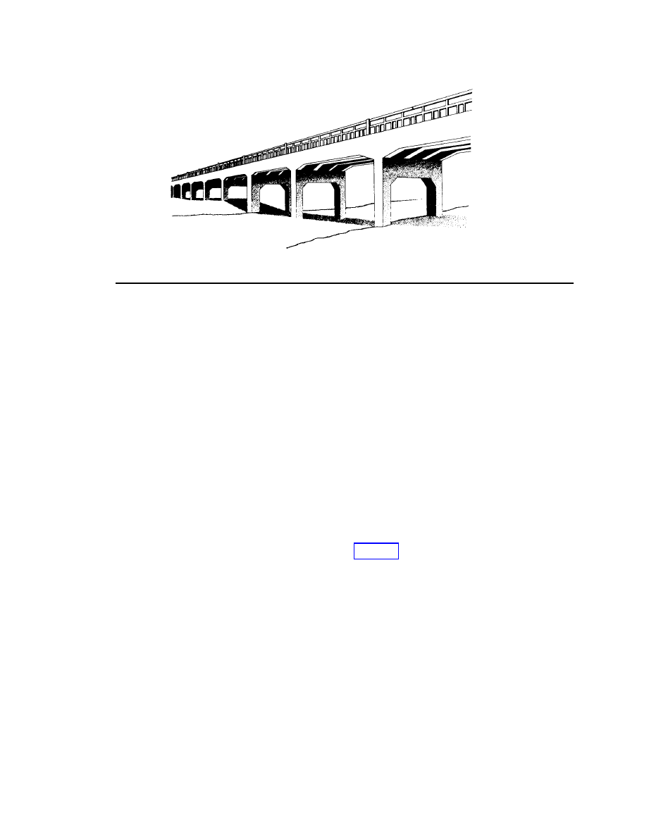
PART TWO
Analysis Procedures
F M 5 - 3 3
Man-made Features
Chapter 4
Transportation Identification
Using a 1:50,000 scale map of the area, register the mylar to the base map and
annotate the marginal information.
Roads
Step 1.
Use the legend of the base map to locate the road classification and type
of route. The route identification numbers will be located astride each road inside
the route symbol. In some areas where the local government does not assign the
roads identification (ID) numbers, you will need to assign arbitrary numbers.
Step 2.
Trace all road segments onto the overlay using the proper symbol for
each road classification. While tracing each road, look for points where either the
classification or ID numbers change. Place a mute symbol at each point of change
and annotate the classification and ID numbers as needed. As you trace each road,
consider that interstate and federal routes do not change when crossing state or
county boundaries. State roads change both classification and ID numbers when
crossing state boundaries, and county roads either change classification or are
terminated when crossing county or state boundaries. See Figure 4-1.
Step 3.
Carefully study the base map legend and compare it the 1:50,000
(TTADB) and 1:250,000 (PTADB) product specifications to determine which
factor overlay symbol to use for each map symbol.
Step 4.
The surface material of each road is located in the legend across from the
appropriate classification symbol. Determine which base map symbol is used in
making the factor overlay and record the feature for each symbol in the legend of
the factor overlay.
Step 5. Determine the
width of the traveled way. Your accuracy in this will vary
with the topographic map available. The FRG, USSR, and other European maps
indicate the width in meters, but US maps indicate it by the number of lanes or a
range of widths. Each road segment between intersections is assigned a width
4-1
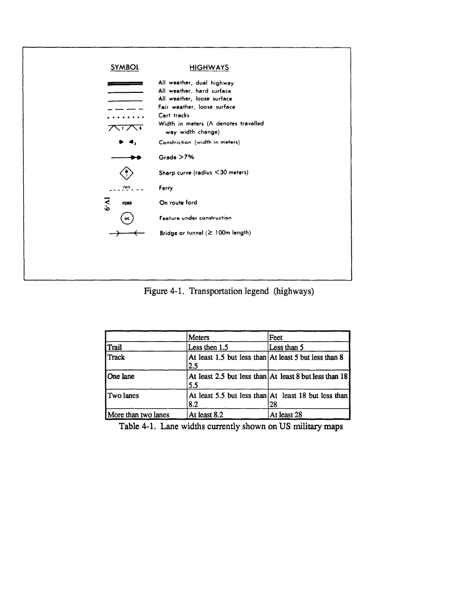
FM 5-33
Analysis Procedures
PART TWO
Note: Only a representative
pattern of major through routes
and secondary roads are an-
notated.
value, with that number placed parallel to the road segment. Table 4-1 below
indicates lane widths currently shown on US military maps.
Follow
each route and determine the number of lanes and widths. Convert the
lane width to meters to indicate the minimum width of the traveled way. Lightly
record this value along the road outlined on the overlay.
Always use a decimal point when recording the road width, for example, 5 meters
= 5.0 meters. Assign each road segment between intersections a width value, then
place that number on the road segment. Note every point at which a change in
width occurs and place a segment symbol at each of those points.
4-2

PART TWO
Analysis Procedures
FM 5-33
When dual routes occur, indicate the width of each route. If the source map gives
only the overall width, assume each side has half the width.
Step 6.
Depict gradient or percent of
S
lope on the overlay when it exceeds 7
percent. The flat end of the first arrowhead is at the bottom of the grade, and the
point of the last arrowhead is at the top. Measure the gradient from the topographic
base map.
To determine percent of slope, measure the change in elevation (vertical distance
or rise) and divide it by the horizontal distance (run), then multiply by 100.
Rise x 100 = percent slope
Run
Step 7.
Show a constriction when the road narrows to less than 4 meters. Indicate
the width measurement adjacent to the arrowhead symbol.
Step 8.
Record all sharp curves with a radius of 30 meters or less.
Step 9.
Depict all features that are currently under construction with the circled
symbol UC.
Step 10.
UTM coordinates are given for key reference points and features. See
FM 21-26, which discusses map-reading instructions.
Bridges, Tunnels, Galleries, and Snowsheds
Step 1. All
bridges are not usually drawn to their true scale on US military maps.
Bridges less than 100 meters long are shown as point features, and bridges greater
than or equal to 100 meters are symbolized by wing ticks. The only bridges not
shown are located on roads that are not depicted. Plot the length between wing
ticks to scale; minimum length between wing ticks is 2.0 millimeters. Point
features are less than or equal to 2.0 millimeters. Draw all other features to scale.
To determine the true length of a structure, use a microcomparator and measure
the feature. Multiply the length of the feature as measured by the microcomparator
using the map scale to get the feature length. Record all structure lengths in the
data table.
Step 2.
Determine structure width. Using the road symbol, establish the width
of all structures of one or more lanes directly from the map. For tunnels and fords,
use only half the width indicated by the symbol, unless other information sources
indicate differently. This width reduction is necessary because some structures are
built with only one lane to reduce the cost of construction. See Figure 4-2.
4-3
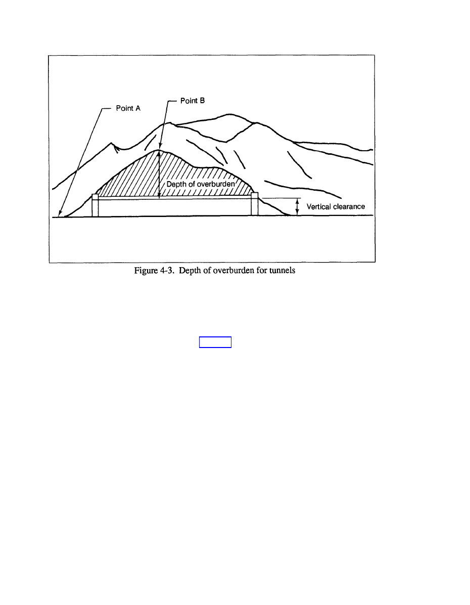
FM 5-33
Analysis Procedures
PART TWO
Step 3.
Determine the depth of overburden. The depth of the tunnel overburden
has tactical significance due to the ability to render road or railroad routes
impassable to tactical units, especially if bypass capabilities are restrictive. Tunnel
overburden is the material, such as soil and rock, that is directly over the tunnel
structure. See Figure 4-3. You can obtain true depth determination of the tunnel
overburden only by ground measurements or from DA Form 1250, Tunnel Recon-
naissance Report. See Figure 4-4. You can estimate depth using aerial photog-
raphy or mensuration techniques. The least effective method is to use contour lines
on a topographic map. If using a topographic map, the maximum depth of the
material (for example, soil or rock) laying directly over a tunnel can be estimated.
a. Determine the elevation of the road surface where it intersects with each tunnel
portal. Select the portal with the lowest elevation.
b. Locate the highest contour line that passes directly over the tunnel symbol and
determine its elevation.
c. Subtract the elevation determined in Step 3a from the elevation determined in
Step 3b. This number is an estimated depth of the tunnel overburden. Record it
on DA Form 1250 as an estimate.
Step 4.
Determine bypass conditions of bridges. You can determine bypass
conditions from a detailed study of the total area extending a distance of 2
kilometers on either side of the bridge. Look for the following factors when
evaluating bypass conditions: steepness of bank slopes, depth of water, denseness
of vegetation, roughness of surface, presence of boulders or approaches, and wet
or soft ground.
4-4
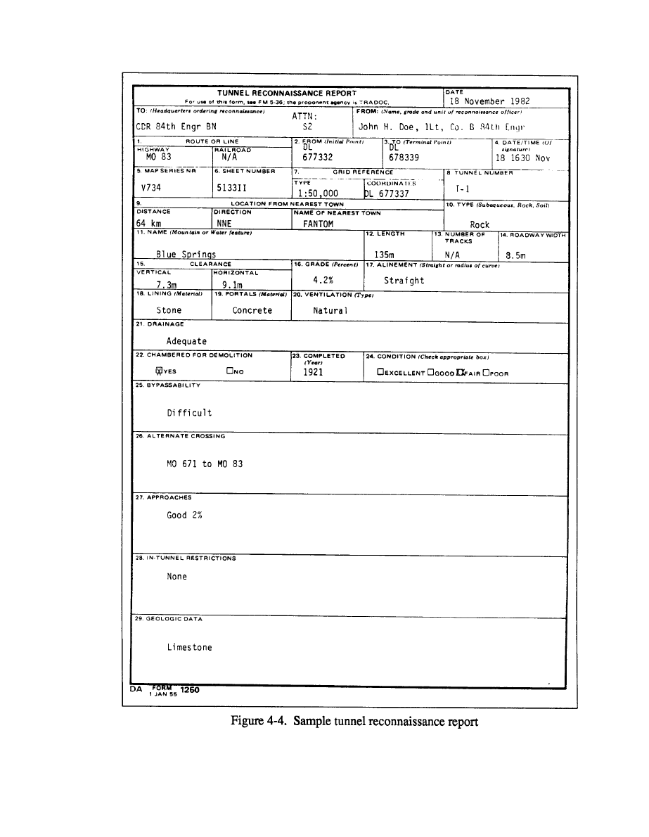
PART TWO
Analysis Procedures
FM 5-33
4-5
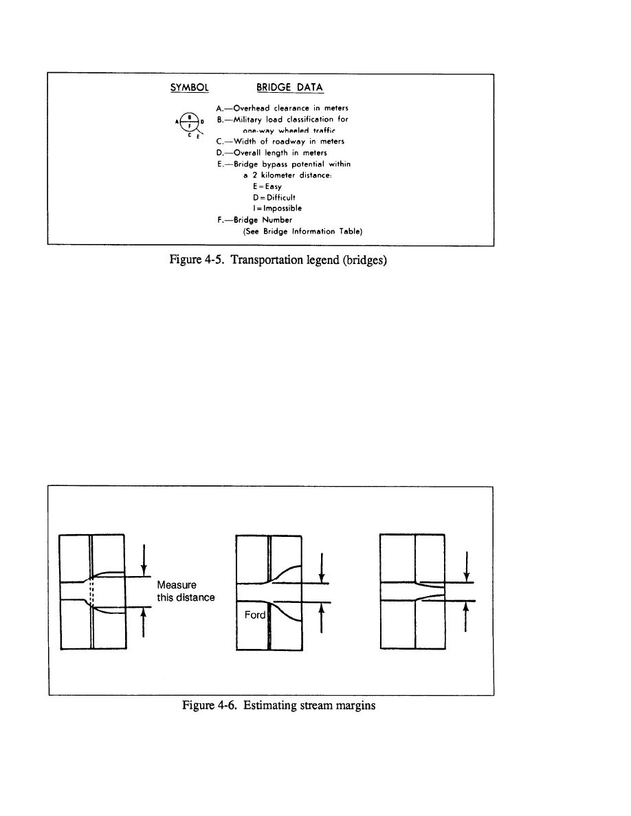
FM 5-33
Analysis Procedures
PART TWO
Identify each bypass as easy (E), difficult (D), or impossible(I) on the line
extending from the NATO bridge symbol to the map location. Easy obstacles can
be crossed within the immediate vicinity of the bridge by a US 2 l/2-ton 6 x 6 truck
(or NATO equivalent) without improving the bypass. Difficult obstacles can be
crossed within the immediate vicinity of the bridge, but some work will be
necessary to prepare the bypass. Impossible obstacles can only be crossed by
repairing the existing bridge or constructing a new bridge. See Figure 4-5.
Fords
A ford is a location in a water barrier where the physical characteristics of the
current, bottom, and approaches permit the passage of personnel and/or vehicles.
Estimate the crossing length of a ford from the map symbol by measuring the
distance between the stream margins. Streams that show only one line are 25
meters or less in width and cannot be used as fords. See Figure 4-6.
4-6

PART TWO
Analysis Procedures
FM 5-33
Divide estimated length by 1,000 to change the length to meters.
Ferries
Step 1.
Determine travel distance. You cannot determine the actual distance of
ferry travel by analyzing the map, because the route indicated on the map is usually
an approximation. When ferry terminals are directly opposite each other, you can
use the width of the river as an approximate travel distance. If the terminals are
located on different maps, determine the straight line open water distance and
record it on DA Form 1252, Ferry Reconnaissance Report.
When you ap-
proximate distances, note this fact adjacent to the length in the reconnaissance
report.
Step 2.
Sketch the dimensional plan of terminals. US military maps often
indicate the plan view of large ferry terminals. Sketch the dimensions of wharves,
buildings, and parking lots in plan view on the ferry reconnaissance report indicat-
ing all true distances.
Airfields
The four types of data shown for airfields are length, width, pavement status, and
orientation.
Step 1.
Trace over the runway to show which direction the runway is oriented.
At the end of each runway, indicate its azimuth to the nearest 10 degrees by
dropping the zero from the numerical value and deriving a one- or two-digit
number. For example, if the azimuth is 260 degrees, the number recorded on the
runway is 26. Record the azimuth on the overlay.
Step 2.
Measure the length and width of the runway using the map scale. If the
runways are not wide enough to permit this procedure, you may place the numerals
immediately adjacent to the runway. The runway length measurement should
exclude the overrun area. Add the information as to whether the runway is paved
(P) or unpaved (U), if you know it. See Figure 4-7.
Heliports
Heliports with runways offer evidence that they are designed for heavier wheeled
cargo or passenger helicopters, while helipads accommodate rotary wing aircraft
4-7
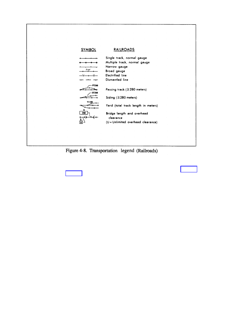
FM 5-33
Analysis Procedures
PART TWO
that do not require a takeoff ground run to become airborne. Label the azimuths
of heliports that have distinct runway orientation. Record the dimensions for width
and length using the map scale and the procedure shown above in Step 2 of
Railroads
Step 1. Determine the correct category from the map legend for railroads and
select the proper symbol for each type. Then draw the railroad symbol on the
overlay for each railroad in the same category. Follow the railroad throughout its
length on the map, looking for points at which either the category
or the ID number
changes. Position the symbols to conform with mapping standards. See Figure
4-8.
Step 2.
Examine the map and legend and determine the track route, gages, and
locations of bridges, facilities, and crossings. Note tunnels and spurs as well as
suspected crossings.
Step 3.
Start tracing the alignment of the railroad across the entire sheet.
Continue this process until you have traced all railroad tracks onto the overlay.
Where the tracks intersect with a built-up area, continue tracing the railroad through
the area. Mark lightly all pertinent features such as bridges, tunnels, and crossings.
If the sheets show a track siding, trace it to its end. Measure the length of the siding
in meters and record it on the overlay. If the siding has a building or facility
indicated or suspected, trace and annotate its location. Certain facilities may
sometimes provide electrical tracks for their privately-owned siding or spur. The
4-8

PART TWO
Analysis Procedures
FM 5-33
track may also become multiple along the siding or spur, if so, you must note this
on the overlay.
Step 4.
Whenever the route crosses a stream or creek, note the possibility of a
culvert on the overlay. You must also identify all road or highway crossings on
the overlay, using the proper symbol.
Step 5.
Rarely will a railroad grade exceed 3 percent. If the contour interval
suggests a greater gradient, note this on the overlay. A slope overlay may be
available with the surface configurat.ion overlays, if previously compiled.
Step 6.
Locate and trace all railroad cut and fill areas. Much of this data will be
deleted from the final overlay. Cuts are potential railroad traffic interdiction sites
because of the possibility of slides induced by demolition of steep side slopes.
Step 7.
Railroad bridges are normally symbolized on topographic maps. Unfor-
tunately, the type of bridge or construction material is seldom stated. Locate all
highway bridges that intersect the railroad route, as well as all railroad-carrying
bridges. Draw the bridge symbol on the overlay adjacent to the site. Measure the
bridge length in meters and note. This will be relevant bridge data for DA Form
1249, Bridge Reconnaissance Report.
Step 8.
Identify the railroad structures. The map legend or map area may have
printed data labeling various railroad facilities such as water towers and switching
pits.
PHOTO ANALYSIS OF TRANSPORTATION
Oblique Aerial Photography
The scale of oblique photography is difficult to determine, because it constantly
varies from the foreground to the background of the photo. If vertical aerial
photography is not available and you must use oblique photography to obtain the
necessary data, consult the appropriate references.
Aerial Photographic Measurements
Step 1.
Determine horizontal measurements. With a magnifier, carefully
determine the location of the traveled way of the bridge. Determine the distance
between the curbs of the traveled way with the microcomparator, and take the
measurement using the metric scale. Multiply the image measurement by the photo
scale to determine the true measurement. Record this value on the bridge cross-
sectional sketch on DA Form 1249. Determine the length of bridge number 1 by
first locating, under stereo viewing conditions, the abutments at each end of the
bridge. With the microcomparator, measure the distance between the abutments.
Multiply this image distance by the photo scale and record it at the proper place on
your sketch. If the bridge is composed of a number of spans, record them on the
sketch and in the Bridge Reconnaissance Report.
Step 2.
Determine vertical measurements. Obtain vertical measurements, such
as the vertical clearance of the bridge and the under-bridge clearance, from stereo
aerial photography by using a parallax wedge or bar. Measurements made with
these instruments are more accurate than those obtained from a map, but they are
4 - 9

FM 5-33
Analysis Procedures
PART TWO
not as accurate as those obtained from on-site measurements or from as-built
drawings. Record the distance on the cross-section sketch on the Bridge Recon-
naissance Report.
Step 3.
Determine under-bridge clearance. Determine the under-bridge
clearance (using the same method) by measuring the difference in elevation
between the bridge deck and the surface of the feature passing beneath the bridge.
Since the bridge substructure will not be visible to you, you will need to estimate
the height of the substructure and subtract it from the computed under-bridge
clearance distance. Record the under-bridge clearance distance on the sketch on
the Bridge Reconnaissance Report.
Step 4.
Determine height. Use the parallax bar to determine height. Orient
photos and secure them with tape.
Surface Materials and Conditions
Step 1.
Estimate surface materials. Figure 4-9 lists the general air photo
characteristics of road surface materials. Compare the photo appearance with the
table, and estimate the surface material during the map analysis. Consider the route
category when the type of material is not readily apparent. For example, national
routes are usually concrete or bitumen, while country roads are often gravel.
Step 2.
Estimate surface conditions. Surface condition is difficult to estimate
except from very large-scale photography. Look for evidence of frequent patching,
checks, broken edges, potholes, ruts, and frost or heat heaving.
Step 3.
Determine surface materials of medians and shoulders. These materials
may be bare ground, grass, trees, shrubs, gravel, bitumen, or concrete. In some
instances, the median may be only a wall or barrier and will be difficult to detect.
Therefore, use the largest photos and the highest practical magnification available.
Bridges
Step 1.
Identify structure features, using oblique photography. Because they
provide aside view of the structure, oblique photos are the best some to determine
construction type, material, length, overhead and under-bridge clearances, number
and type of span, and length of individual spans. Measurement is dependent on
careful, accurate determination of the scale. When practical, make duplicate
measurements on vertical photography and average the results.
Step 2.
Measure bridge features using vertical photography. Measurements on
vertical photos are usually more accurate than similar measurements made on
oblique photographs, but vertical photos do not provide the side view so useful in
determining the type of construction. A definite shadow of the bridge often
provides much of the same information available from oblique coverage. When
no shadow of the bridge exists, examine the surrounding vertical photographs and
look for an image of the bridge that falls near the edge of the photograph. Images
near the edge of vertical photos are often displaced or tilted so that the side of the
object is visible.
Step 3.
Determine the military load class. You cannot determine the military load
class directly from aerial photography, but you can roughly estimate it from
vehicles that were using the bridge at the time the photo was taken. Examine the
4-10
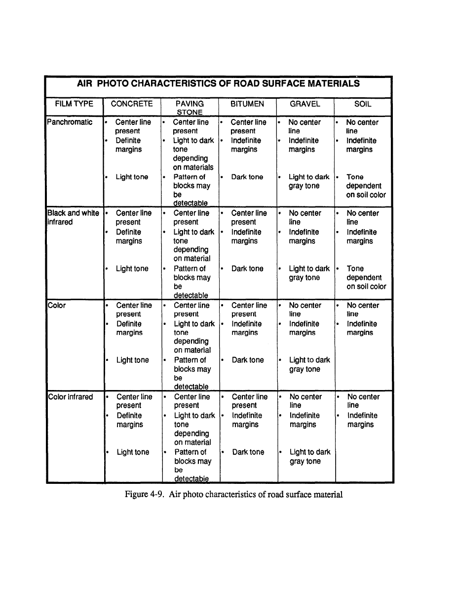
PART TWO
Analysis Procedures
FM 5-33
4-11

FM 5-33
Analysis Procedures
PART TWO
photos and identify any vehicles on the bridge. If you can estimate the load class
of the vehicle, you can assume that the class of the bridge is at least the same. If
no vehicles are actually on or approaching the bridge, the load class cannot be
estimated.
Step 4.
Identify construction type and materials. On large-scale aerial photog-
raphy (1:2000 to 1:15,000) such as panchromatic and color, you can easily identify
construction type and materials such as masonry, wood, steel-reinforced concrete,
and steel by indicators on the photos. These indicators include shadow and
photographic tone, color, and texture. With detailed study of the photographs,
especially under stereo conditions, you should be able to determine not only the
type of construction but also the major structure composition.
Step 5.
Determine bypass conditions. The standard topographic map will supply
all the necessary information to determine bypass conditions for each bridge and
LOC structure. However, you must use aerial photography to continuously update
the map, particularly under combat conditions. To determine bypass conditions
from aerial photography, study the area adjacent to the structure under stereo
conditions and note any indications of shallow water, such as sandbars or rocks,
that are visible through the water surface. In addition, look for vehicle tracks along
the river bank that indicate the location of an existing ford. When the structure is
a dam used as a bridge, examine the downstream side of the dam, where the water
is often shallow enough to be used as a bypass. Because dams are almost always
situated where bedrock is close to the surface, stream bottom conditions are usually
firm enough to support most vehicle types.
Ford Width
Look for indications that the roadway continues across the channel, such as two
faint lines that mark the sides of the traveled way. On some fords, the sides of the
roadway are marked by boulders that appear on the imagery. Where the ford has
been raised by adding material to the bottom of the stream, the sides may appear
as lines of ripples or as eddies of a lighter tone than the surrounding water. Measure
the width.
Ford Bottom Characteristics
Determining ford bottom characteristics such as paved, rocky, and sandy from
aerial photography depends on a number of factors. They include water depth and
clarity, film type, and photo scale. To determine this data, orient aerial photos of
the ford for stereo viewing using proper procedures. Study the area around the
ford, as well as the river or stream channel both upstream and downstream of the
ford.
Rapids, white water, and exposed rocks or boulders indicate a rocky bottom.
Bars, braiding, and steep banks often indicate coarse-grained material such as sand
or gravel. Meanders and oxbows in the immediate vicinity indicate relatively
slow-moving streams with fine-grained material. Angular drainage patterns with
frequent sharp changes indirection indicate rock control and a rocky bottom. In
swift-flowing streams in mountainous areas, fine materials do not settle; therefore,
the bottoms are usually rocky or firm.
4-12

PART TWO
Analysis Procedures
FM 5-33
Length of Ferry Crossing
You can easily determine ferry crossing length from aerial photography if both
terminals appear on a single photograph. If two or more photos are required,
construct a mosaic of several photos.
Single Photo Method
Determine the scale of the photo, using proper procedures. Locate terminals and
measure the open-water distance between terminals with the microcomparator or
PI scale. Multiply the measured distance by the denominator of the representative
fraction to determine true distance.
Mosaic Method
Determine the number of photos required to cover the entire open-water distance
between ferry terminals. Secure the photo containing the most western terminal to
a suitable flat surface. Carefully place the adjacent photo over the edge of the first
photo, aligning common terrain features of Photo 2 with Photo 1. Continue this
process until the second ferry terminal appears on a photo. Check your work,
making certain that all photos are properly aligned.
Scale the open-water distance between ferry terminals. Multiply the photo
distance by the denominator of the photo representative fraction.
Ferry Terminal Layout
Step 1.
Orient the photos for each terminal, using proper procedures, and
examine the terminal facilities and approaches.
Step 2.
Examine the land facilities. Look for large buildings, parking lots,
winches, guy-line towers, and any other features that may affect the use or capacity
of the site. When feasible, determine the dimensions of the site and major
structures.
Step 3.
Examine the water approaches. Look for obstacles, fenders, piers,
pilings, and evidence of the channel.
Step 4.
Analyze vessel information such as ferry length, beam, and capacity. To
do so, you will need to orient photos, locate one or more of the vessels, and
determine the photo scale. With the microcomparator, measure the length and
width of each vessel. Multiply the photo distances by the denominator of the photo
scale to determine true distances.
Step 5.
Estimate the number of vessel decks capable of carrying vehicles.
Assume an automobile size of 2 by 6 meters and a weight of 2 tons.
Step 6.
Estimate vehicle capacity for one deck of the vessel. Multiply this
number by the number of decks. If all vessels do not have the same length and
beam, measure and record each vessel separately.
Step 7.
Examine approach conditions for fords and ferries. Approaches are
classified as easy when the slope is 7 percent or less; the surface is relatively smooth
with no ruts, potholes, or other obstacles; the width is at least 3 meters; there are
no sharp curves within 50 meters of the water’s edge and the surface is well drained
4-13
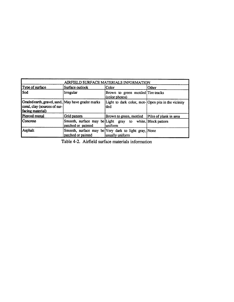
FM 5-33
Analysis Procedures
PART TWO
or free of standing water. Failure to meet all of these conditions will result in the
approach being classified as difficult.
Airfields
Step 1.
Using the PI and photographic scales, measure the length and width of
the runway. Record the measurements in meters on the factor overlay within the
runway boundary lines or beside the runway.
Step 2.
Determine the surface material of the runway using the information in
Table 4-2. Label runways with hard or paved surfaces with a P, and loose or
unpaved surfaces with a U..
Step 3.
At most major airfields, the magnetic alignment of runways is painted in
large numerals at the ends of the paved surfaces. These azimuths, contrasting with
the runway coloration, may be legible on aerial photography. Transfer these values
to the ends of runways shown on the factor overlay. If the numerical designations
of runway azimuths do not appear or are illegible on the photography, measure the
magnetic orientation of each runway and enter the values at the ends of the runways.
Railroads
Step 1.
From the stereo pairs, locate the area of the railroad to analyze. Compare
the date of the photographs with the date of the last map revision or update. If the
photographs are more recent than the map, use them. If the map is more recent,
give greater weight to the map information however, even if it is more recent, it
should not always take precedence over the photographs, because map information
is often general. As a result, some feature such as sidings are not shown.
Step 2.
Look for any railroad sidings not shown on the map. Compare the outline
of all built-up areas on the photos with the map symbols of the same areas. Lightly
sketch any new alignments or built-up areas onto the overlay in pencil.
Step 3.
Verify the location of each segment end point. If the end points
determined from the photo differ from those obtained from the map, use the points
obtained from the photos. Relocate the endpoint symbols on the overlay, renumber
the segments
if necessary, and determine the coordinates of the relocated points.
Change entries in the railroad data tables if necessary.
4-14

PART TWO
Analysis Procedures
FM 5-33
Step 4.
Verify the gradient of each segment that has a grade of 3 percent or
greater.
Step 5.
Examine aerial photography to verify the location of culverts or streams.
The map indicates the location of culverts or streams passing beneath the railroad.
Also check all areas on the photos where a stream or drainageway intersects a
railway. If these areas indicate culverts, annotate the overlay at each location.
Make notes in the data tables as necessary.
Step 6.
Locate built-up areas on aerial photos that show railway through-routes.
Locate any zones where buildings, walls, and so forth constrict the width of the
route to less than 4 meters. Measure the constrictions, using the microcomparator
or the PI scale, and record the data in the proper place on the overlay.
Step 7.
Examine and verify areas previously identified as level crossings. Make
additions, deletions, or changes on the overlay as required.
Step 8.
Determine catenary clearance. The clearance beneath the catenary is
required only if the railroad understudy is electrified and uses overhead wires. The
catenary clearance is seldom shown on maps. Photos may provide some indication
of catenary clearance. If not, place a question mark above the crossings on the
overlay to indicate there are overhead wires but the clearance is unknown.
Step 9.
Assemble the vertical photos that provide stereo coverage for each bridge
recorded on the factor overlay. If oblique photos are available, place them with
the vertical ones. Study the material carefully to become familiar with the general
characteristics of the bridge. Determine the number of spans, overhead clearance,
and so forth. Measure the roadbed widths. Record all data in Railroad Date Table
2 or annotate it on the overlay.
Inland Waterways
Classify inland waterways according to their depths. Very shallow waterways
have depths less than 1.4 meters. Medium waterways have depths between 1.4 and
2 meters. Deep waterways have depths greater than 2 meters. See Chapter 2 for
more information.
Facilities and Installations
Step 1.
Identify all wharves. Figure 4-10 shows a reference diagram of a wharf.
Step 2.
Identify all locks. Common types of leeks are single and multiple-cham-
ber. See Figure 4-11. Gates are the most vulnerable features of a leek. Common
types of gates are--
Double-leaf miter gates (see Figure 4-12). A pair of hinged gates that
form a V or angle across the end of the leek when closed. The apex is al-
ways upstream to use the head of water to keep the gates closed.
Single-leaf miter gates. Hinged gates that pivot into a recess in the lock
Vertical-lift gates. Lock gates that move in a vertical plane. Those gates
are usually suspended from an overhead frame and counterbalanced.
4-15
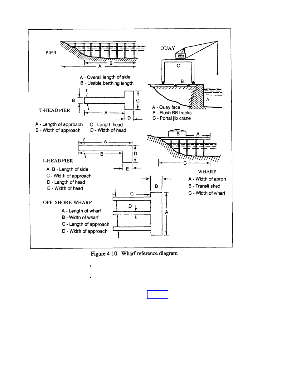
FM 5-33
Analysis Procedures
PART TWO
Caisson or sliding (retractile) gates. Those gates move horizontally into
wells or caissons when open.
Segmental gates. A pair of gates shaped like sectors of a cylinder. They
are hinged at the sides and rotate into wells.
Step 3.
Prepare final overlay. See Chapter 8 for procedures.
4-16
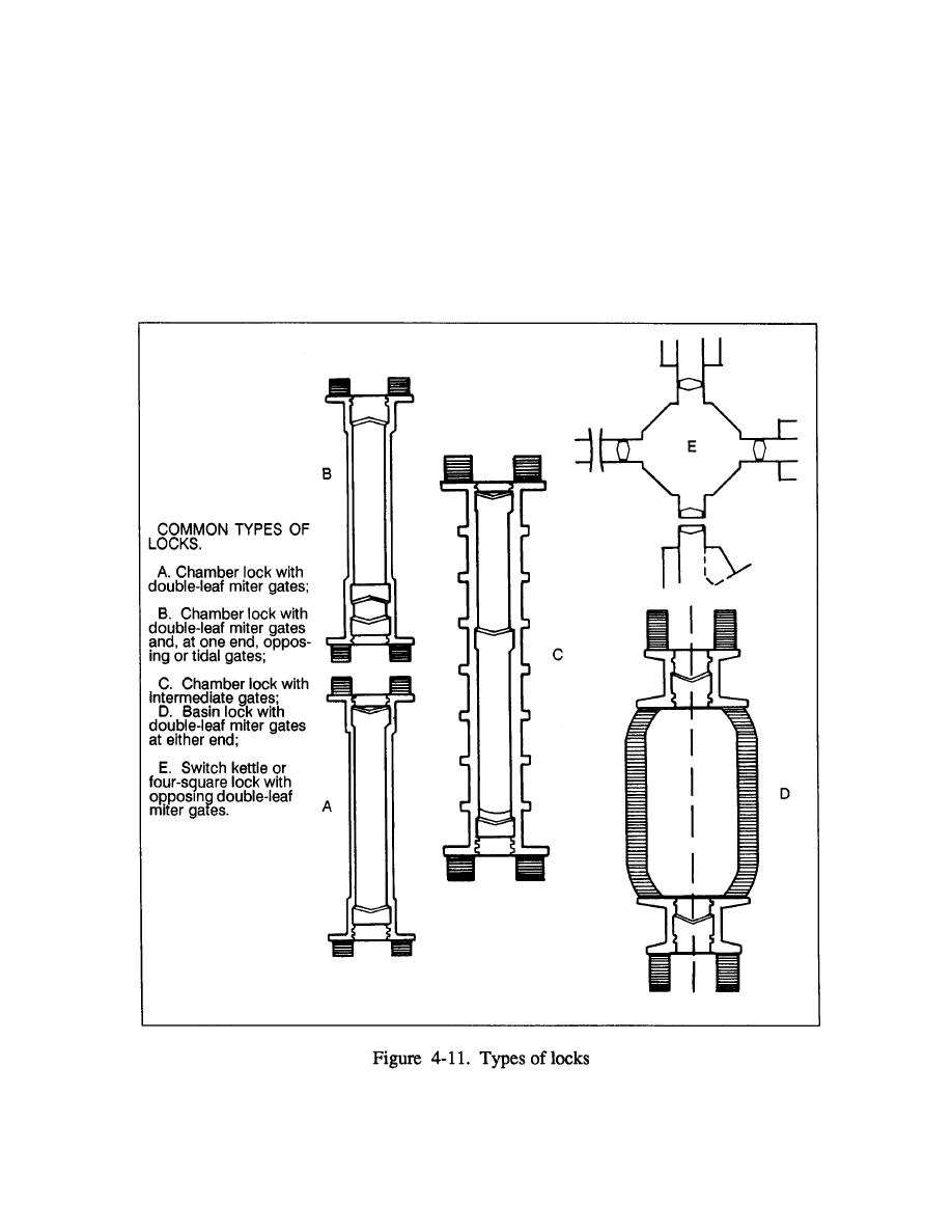
PART TWO
Analysis Procedures
FM 5-33
URBAN AREAS
Step 1.
Obtain a 1:50,000-scale map covering the area of interest. Register the
mylar to the map or data base and annotate the marginal information. Then locate
and outline all areas that cover the area to be studied.
Step 2.
Establish a numerical priority listing (ranking) of urban areas to be
analyzed at a scale of 1:12,500. Determine this sequence based on whether the
areas are administrative centers (state and national capitals, strategic centers of
4-17
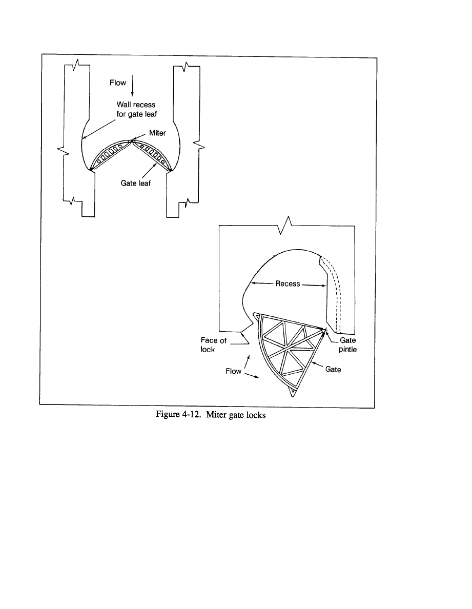
FM 5-33
Analysis Procedures
PART TWO
production, steel, manufacturing, and nuclear power plants), or are located on
dominant ground or on major avenues of approach.
Step 3.
Assign a priority number to each urban area and carry out the analysis
accordingly. Where all urban areas on a 1:50,000-scale map are to be analyzed
without concern for priority consideration, number each area, beginning at the top
left corner of the identification overlay, and proceed across and down the map.
Step 4.
Retrieve a 1:12,500-scale topographic map of the urban area. If you
cannot find any, outline the desired area on the 1:50,000-scale map and enlarge this
map segment by 400 percent. If a 1:25,000-scale map is available, you may enlarge
4-18

PART TWO
Analysis Procedures
FM 5-33
it by 200 percent. The enlarged map will become the base map to which all factor
overlays will be registered.
You will require multiple overlays to extract information for the data fields
documented in order to map adequately the diverse terrain features that makeup
the urban area. In this regard, the number of overlays to be used is considerably
greater than the number used in other areas. Some topics include vegetation, roads
and related structures, drainage and water resources, and railroads and related
structures. Because of the larger scale of the urban-mea products and the com-
plexities inherent in this unique terrain, some elements are portrayed differently
from those depicted on overlays keyed to 1:50,000-scale maps.
Step 5.
Determine the area to be analyzed and gather all necessary aerial
photographs in stereo pairs to cover the area. Orient them for stereo viewing.
Step 6.
View the photographs in stereo and use the PI keys and text to determine
the urban type in the aerial coverage. Then analyze, outline, and identify all types
and label them with the appropriate urban code.
Step 7.
Determine the roof coverage. Density refers to the ratio of roof area of
buildings to total ground area, including streets and small open spaces. To
determine roof cover percentage from aerial photography, collect the necessary
stereo pairs for the area to be analyzed and note the photo scale. Measure the
footage of the area, both the length and width, with a thousands-foot scale and
multiply it by the photo scale.
GD = PD x PSR
Area=L x W
Where--
GD = ground distance
PD = photo distance
PSR = photo scale reciprocal
L = length
W = width
Step 8.
Determine the roof size by measuring the average roof in the area the
roofs should all be about the same size. Using the microcomparator, measure the
length and width of an average roof and multiply it by the photo scale. Then count
the number of buildings and multiply that number by the area of the roofs. To
determine the percentage of the roof coverage, take the roof size times the number
of buildings in the area, divide it by the total area, and multiply it by 100.
Total area of buildings x Number of buildings in area x 100 = % Roof coverage
Total area size
Figure 4-13 will help determine the percentage of roof coverage and the percent-
age of concealment from aerial detection. Use the appropriate symbol to mark the
overlay.
4-19
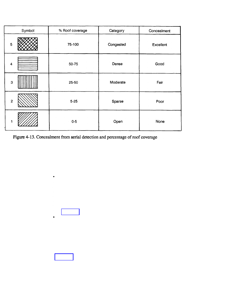
FM 5-33
Analysis Procedures
PART TWO
Step 9.
Determine construction and building type. Make appropriate annotations
for type of construction or building, using the definitions below. Note: Building
types 5 through 8 are comprised of multistory office and apartment buildings. For
the purpose of classification and subsequent evaluation, each category is divided
into low-rise buildings of six stories or less and high-rise structures in excess of six
stories.
4-20
Type 1. Wood and timber frame construction. Most farm buildings and
those buildings constructed prior to the late 19th century are classified as
Type 1. Their ceilings with wooden rafters and weak exterior walls offer
little protection from indirect or direct weapons fire. Internal communica-
tions routes are excellent since their lightly constructed walls are easy to
breach; however, significant reinforcement is required to provide protec-
tive cover if such buildings are to be used as defensive positions. Within
larger built-up areas, Type 1 buildings present the greatest fire hazard.
Type 2. Masonry construction. Buildings with strong walls of brick or
natural stone constructed in the 19th and early 20th centuries are clas-
sified as Type 2. These buildings, typified by the old town hall, are com-
monly found in the central areas of towns and cities. They generally con-
tain from two to four stories with ceilings with wooden rafters and lightly
constructed tile roofs. Presenting less of a fire hazard than wood and tim-
ber frame structures, Type 2 buildings are frequently suitable as defensive
positions. While internal communication routes are excellent, external
walls are difficult to breach without heavy weapons or demolitions. See
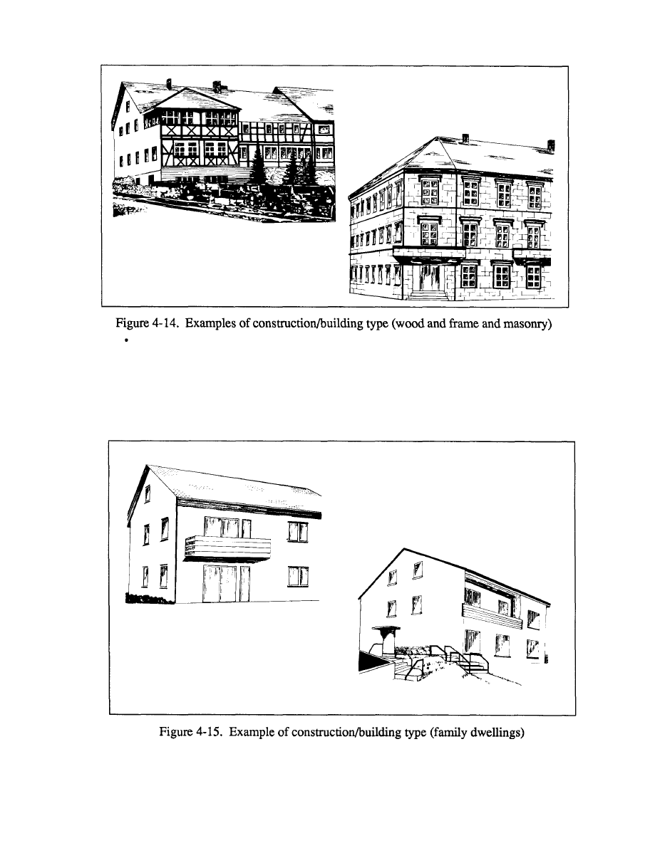
PART TWO
Analysis Procedures
FM 5-33
Type 3. One- or two-family dwellings. Family dwellings constructed of
solid or insulating bricks or of cinder blocks with ceilings of reinforced
concrete are classified as Type 3. Such buildings frequently contain
strongly constructed basements. Type 3 buildings offer significant protec-
tion and require little reinforcement if used as defensive positions.
Because of Type 3 construction, fire hazards are minimal. If demolished,
significant rubble is generated, offering protection to the defender or creat-
ing an obstacle to the attacker. See Figure 4-15.
4-21

FM 5-33
Analysis Procedures
PART TWO
Type 4. Prefabricated one-family dwellings. Prefabricated family dwell-
ings assembled with precast and light building materials are classified as
Type 4. In most cases, the cellars or basements are strongly constructed.
Unlike Type 3 dwellings, these buildings require significant reinforcement
if they are to be used as defensive positions. They also constitute a fire
hazard in a freed defense. Rubble produced by their destruction creates an
effective obstacle and additional cover for ground-level defensive positions.
Type 5. Low-rise office buildings. Multistory office buildings, with their
steel frame and reinforced concrete construction, are normally characterized
by large expanses of plate glass which offer little protection. See Figure
Type 6. High-rise office buildings. These buildings are also characterized
by large expanses of plate glass which offer little protection, but they have
six stones or more.
Type 7. Low-rise apartment buildings. While similar in size to low-rise of-
fice buildings, they generally have smaller glass areas and load-bearing rein-
forced concrete exterior walls which provide greater protection.
Type 8. High-rise apartment buildings. See Type 4, paragraph 2. See
Type 9. Buildings common to newer industrial and warehouse complexes
are classified as Type 9. While the type construction may vary consider-
ably, steel framing and the use of lightweight materials for exterior walls
and roofs are normal practices. Reinforced concrete floors and ceilings are
frequently used in multistory buildings.
Figures 4-17 through 4-31 show examples of industrial areas that will be useful in
identifying specific subdivisions of the industrial classification.
This completes the urban analysis procedure. See Chapter 8 for final overlay
preparation procedures.
4-22
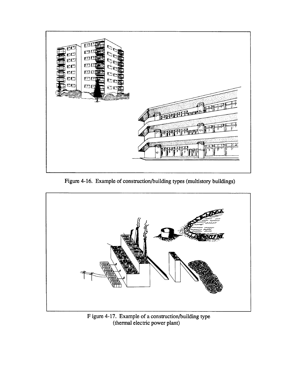
PART TWO
Analysis Procedures
FM 5-33
4-23
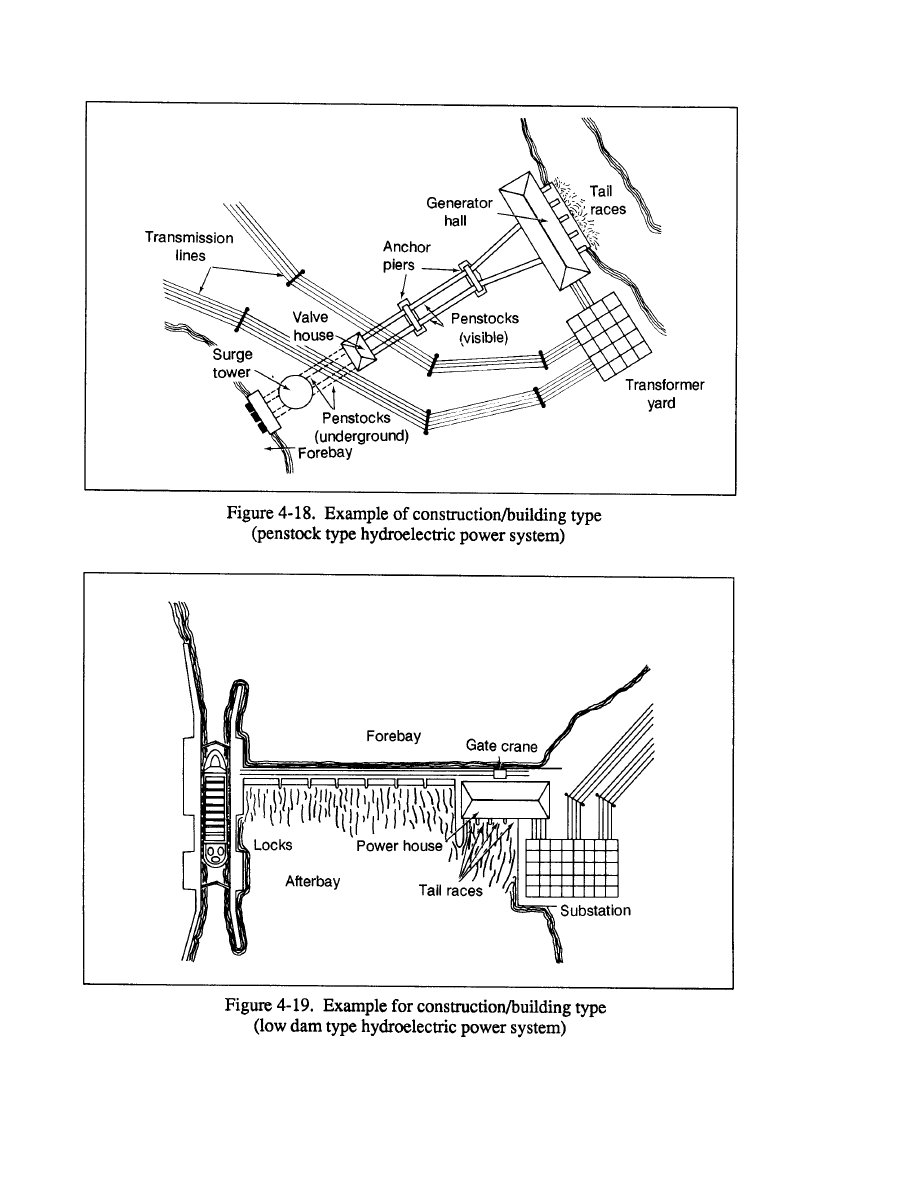
FM 5-33
Analysis Procedures
PART TWO
4 - 2 4
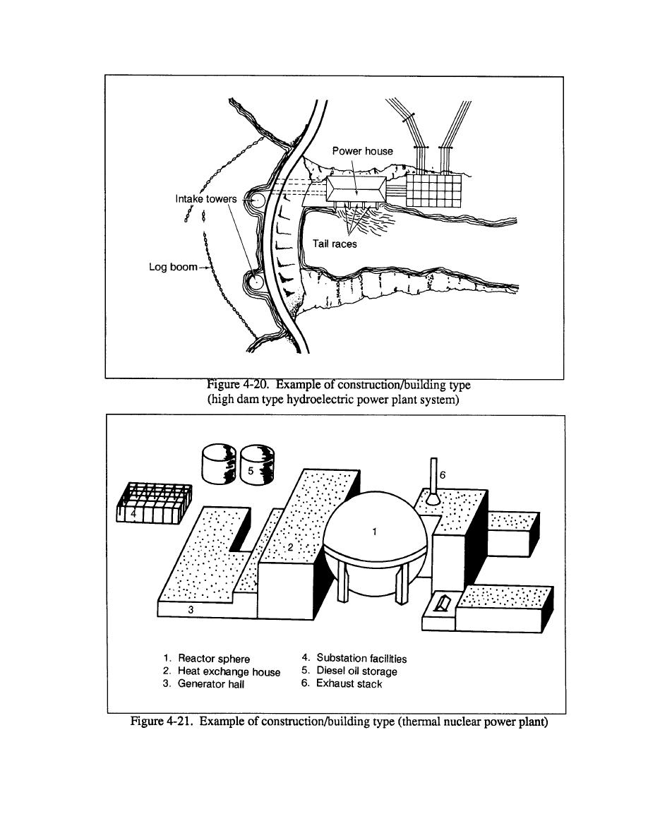
PART TWO
Analysis Procedures
FM 5-33
4-25
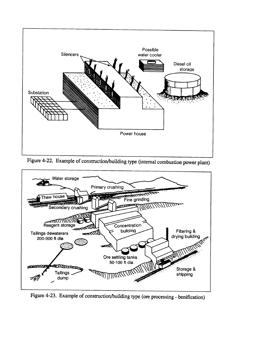
FM 5-33
Analysis Procedures
PART TWO
4-26
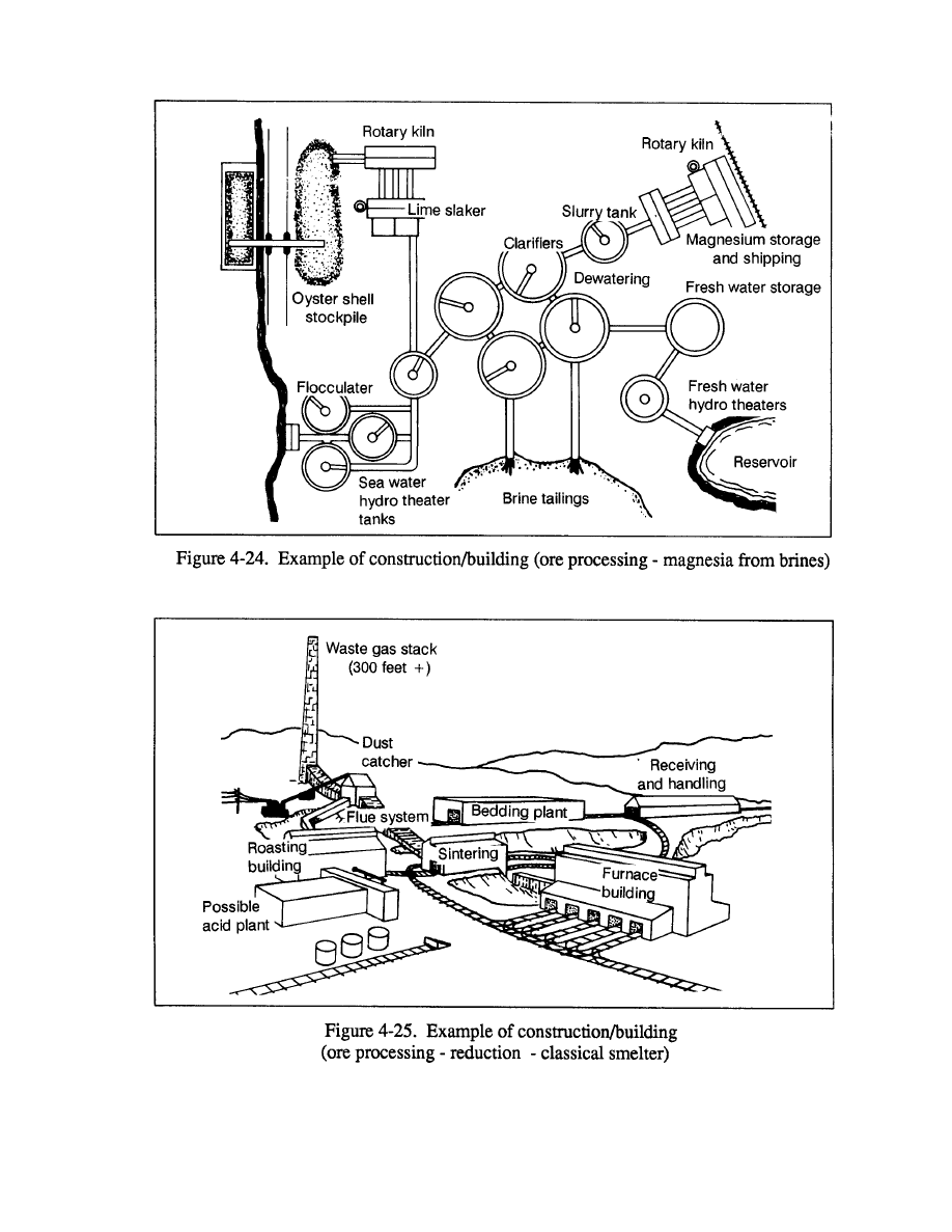
PART TWO
Analysis Procedures
FM 5-33
4-27
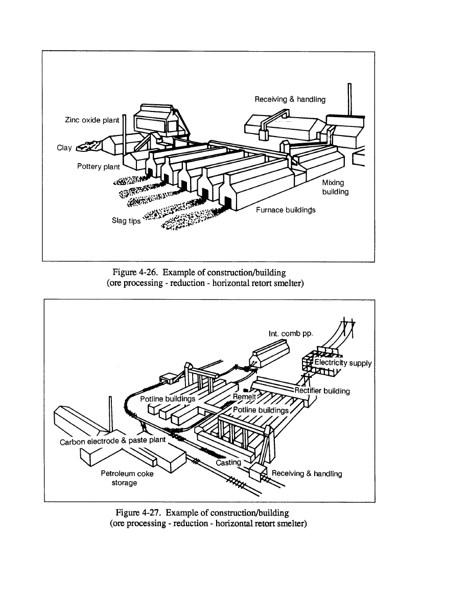
FM 5-33
Analysis Procedures
PART TWO
4-28
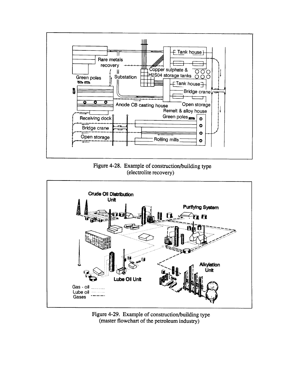
PART TWO
Analysis procedures
FM 5-33
4-29
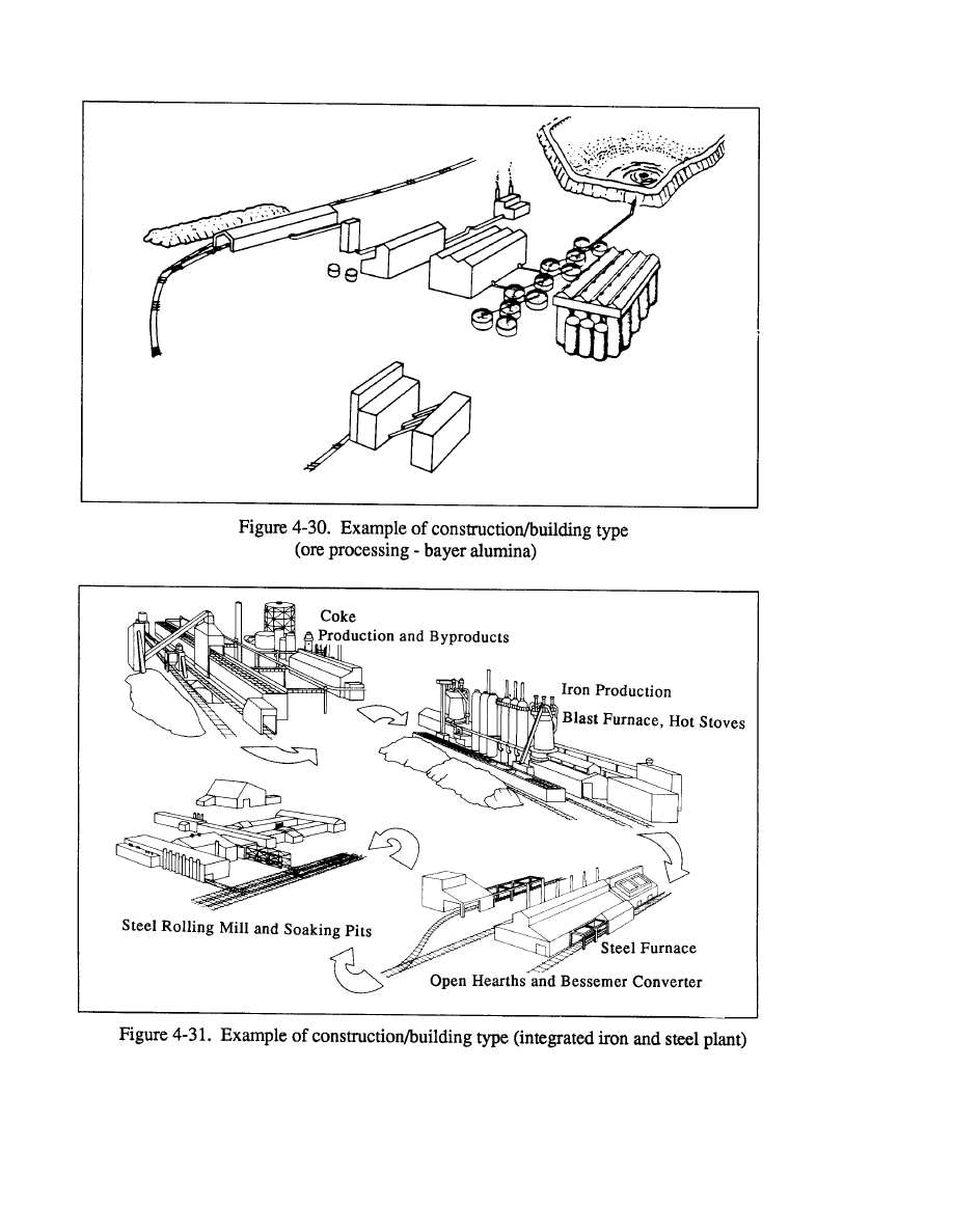
FM 5-33
Analysis Procedures
PART TWO
4-30

FM 5-33
PART THREE
Synthesis Procedures
LINES OF COMMUNICATION,
COVER AND CONCEALMENT
Chapter 5
LINES OF COMMUNICATION
Lines of communication (LOC) are all the routes (land, water, and air) that
connect an operating military force with a base of operations and along which
supplies and reinforcements move. An LOC map is especially important to
transportation corps and logistics personnel. It is also important for planning the
interruption of enemy supplies. This map differs from the CCM map in that it
shows routes over which supplies rather than deployed forces will move, so it
depends more heavily on existing roads, railroads, and airfields.
Roads
Step 1.
Study the requirements from corps and division before preparing
specifications for synthesizing LOC roads.
Step 2.
Examine the base map and become familiar with the LOC study area
road net.
Step 3.
Examine the transportation factor overlay, to select the major and
secondary roads, the on-route fords, ferries, tunnels, galleries, and snowsheds for
the LOC study. Identify major road categories to be used in the LOC study, such
as all-weather hard surface and fair-weather loose surface.
Step 4.
Examine the data tables to select the essential data elements listed on
Step 5.
Obtain aerial photos for the area of interest to verify and update
information.
5-1
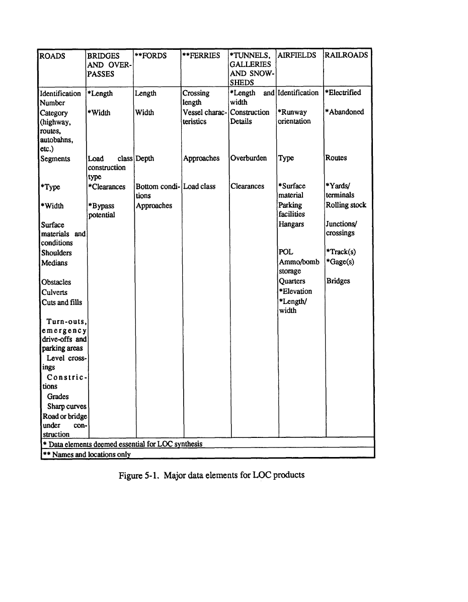
FM 5-33
Synthesis Procedures
PART THREE
Step 6.
Prepare an informal layup from alternate photos. Examine the road
network, correlating the roads selected for the LOC study with the photos. Also
examine the tunnels, galleries, snowsheds, ferries, and on-route fords.
5-2

PART THREE
Synthesis Procedures
FM 5-33
Step 7.
Stereoscopically examine the selected roads, tunnels, galleries, snow-
sheds, ferries and on-route fords to ensure that there are no changes or errors in the
data-base parameter information. Revise and record any changes.
Step 8.
Recheck all gathered information on roads, tunnels, galleries, snowsheds,
ferries, and on-route fords to ensure that the selected roads meet with the user’s
request.
Step 9.
Compile all pertinent data and draft it onto a clean overlay. Make sure
the data pertains to the LOC, since not all data on factor overlays is necessary for
an LOC overlay. See Figure 5-2.
See Figure 5-2 for typical roads and related structures found on a factor overlay.
The data is derived from an analysis of maps, literature, and photos, and the details
for the data elements are recorded on a roads factor overlay data table, which shows
more than you need for a study. After examining the map area and identifying the
LOC relevant data elements, check the available aerial photography of the area.
Bridges and Overpasses
Step 1.
Study the requirements from corps and division before preparing
specifications for synthesizing the LOC.
5-3

FM 5-33
Synthesis Procedures
PART THREE
Step 2.
Examine the base topographic map to become familiar with the LOC
study area.
Step 3.
Examine the bridge section of the transportation factor overlay to select
pertinent information.
Step 4.
Examine the bridge data table to select the data elements listed on Table
1 for each relevant LOC.
Step 5.
Obtain aerial photos for the area of interest to verify and update
information.
Step 6.
Prepare an informal layup from alternate photos. Examine the road
network and locate the bridges selected for the LOC study area.
Step 7.
Stereoscopically examine the selected bridges for any changes or errors
in data-base parameter information. Revise and record any changes.
Step 8.
Recheck all gathered bridge information to ensure the selected bridges
meet with the user’s request. You must show all bridges greater than or equal to
18 meters.
Step 9.
Record only the pertinent information on the draft LOC. See Figure 5-2.
Railroads
Step 1.
Study requirements from corps and division before preparing specifica-
tions for synthesizing the LOC railroads.
Step 2.
Examine the base topographic map to become familiar with LOC study
area railroads.
Step 3.
Examine the transportation factor overlay to select LOC areas of interest.
Step 4.
Examine the railroad data table to select the essential data element
information as listed in Figure 5-3.
Step 5.
Obtain aerial photos for the area of interest to verify and update
information.
Step 6.
Prepare an informal layup from alternate photos. Examine the area
railroads and locate the segments selected for the LOC study area.
Step 7.
Stereoscopically examine the selected railroads for any changes or errors
in data-base parameter information and make necessary revisions.
Step 8.
Recheck all gathered information to ensure that selected railroads meet
with the user’s request.
Step 9.
Outline all information on the draft overlay.
5-4
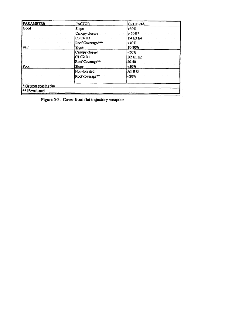
PART THREE
Synthesis Procedures
FM 5-33
Note : Criteria may not be
applicable to your unit.
Airfields
Step 1.
Study requirements from corps and division before preparing specifica-
tions for synthesizing the LOC airfields.
Step 2.
Examine the base topographic map to become familiar with the LOC
study area.
Step 3.
Examine the transportation factor overlay to select pertinent areas of
interest.
Step 4.
Examine the airfield data table to select the essential data elements
information as listed in Figure 5-3.
Step 5.
Obtain aerial photos for the area of interest to verify and update
information.
Step 6.
Prepare an informal layup from alternate photos. Examine the airfields
and locate the segments selected for the LOC study area.
Step 7.
Stereoscopically examine the selected airfields for any changes or errors
in data-base parameters information, and make necessary revisions.
Step 8.
Recheck all gathered information on airfields to ensure that selected
airfields meet the user’s request.
Step 9.
Outline all information on the draft LOC overlay.
Remaining Factor Overlays
Step 1.
Check the soils factor overlay tow what effect soil conditions will have
on unsurfaced routes. Consider the probable weather to see if it might cause
5-5
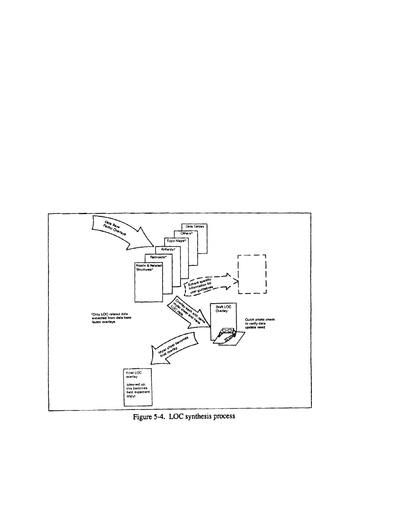
FM 5-33
Synthesis Procedures
PART THREE
surfaces to be muddy, frozen, dry, or dusty and to see if the expected condition will
be favorable or unfavorable to movement along the roads.
Step 2.
Check the vegetation factor overlay and mark any areas where vegetation
will conceal the mute. Show the percent of canopy closure at the given time of
year.
Step 3.
Check the drainage factor overlay to locate and mark areas where
flooding might impede movement, to see if any rivers must be bridged or forded,
and to see what trussing facilities exist. Figure 5-4 shows steps to be followed in
the synthesis process from existing factor overlays and data tables.
COVER FROM FLAT TRAJECTORY WEAPON
Cover, or protection from enemy fire, is a vital part of military operations.
Examples are rocks, river banks, vegetation, quarries, walls, and buildings.
Step 1.
Study requirements from the requester.
Step 2.
Obtain source materials, including the base topographic map, photog-
raphy, and vegetation and slope-factor overlays.
5-6
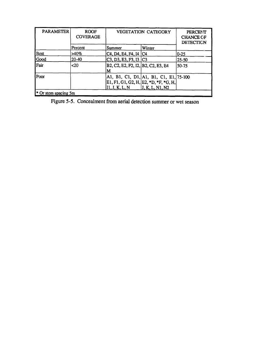
PART THREE
Synthesis Procedures
FM 5-33
Note:
This par-
Step 3.
Review source materials.
Step 4.
Determine what parameters each category falls into (good, fair, or poor).
To construct a cover overlay, you must consider slope, vegetation, and, roof
coverage (if it is evaluated).
Step 5.
Draft the cover overlay.
CONCEALMENT FROM AERIAL DETECTION
Concealment is protection from observation. This overlay is important for
judging where the enemy might be located. It is especially important in areas where
guerrilla forces might be operating, because it helps the commander predict attacks.
Concealment may be provided by woods, underbrush, snowdrifts, tall grass,
cultivated vegetation, roof coverage, or any other feature that denies observation.
Step 1.
Study the requirements and determine if concealment is for the summer
(wet) season or for the winter (dry) season.
Step 2.
Obtain the base map, aerial photography, and the proper seasonal
vegetation factor overlay.
Step 3.
Review the vegetation factor overlay with the base map and aerial
photography to ensure that all vegetation categories are shown correctly. A
deciduous forest with 25 to 50 percent canopy closure is a D2 vegetation code on
the data-base factor overlay and is a fair area for concealment. A mixed forest with
0 to 25 percent canopy closure is an E1 vegetation code on the data-base factor
overlay and is a poor area for concealment. The type of vegetation and the canopy
closure are the two main factors you should check on the vegetation factor overlay.
Step 4.
If evaluated, roof coverage is also used as protection from observation.
You will probably look at this more in winter than summer because of the lack of
vegetation during winter. Use Figure 5-5 to determine which parameter each
vegetation category and roof coverage will fall into.
Step 5.
Draft a concealment overlay.
ticular criteria being
used may not be ap-
plicable to your unit.
It should be revised
to meet your unit
S
specific needs.
5-7
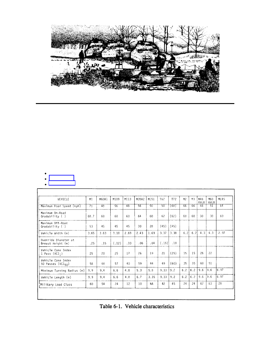
PART THREE
Synthesis Procedures
FM 5-33
CROSS-COUNTRY MOVEMENT
Chapter 6
PREPARE CCM OVERLAY
The cross-country movement (CCM) overlay is sometimes referred to as an
avenue-of-approach map because it tells the best routes by which various vehicles
can get to an objective when they cannot use prepared roads. It also shows parts
of terrain that these vehicles cannot cross.
Step 1.
Assemble source materials. These will include the base topographic map,
aerial photography, slope (surface configuration), vegetation and soils (surface
materials) factor overlays, and the following tables:
Table 6-1, Vehicle characteristics.
Table 6-2, Slope/speed characteristics.
Table 6-3, Soils factor (dry and wet).
6-1
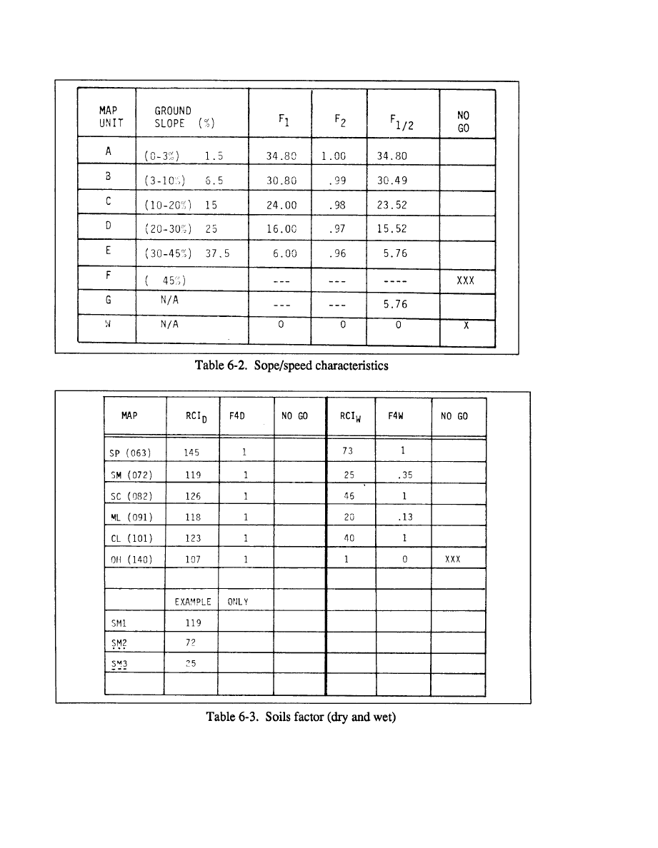
FM 5-33
Synthesis Procedure
PART THREE
6-2
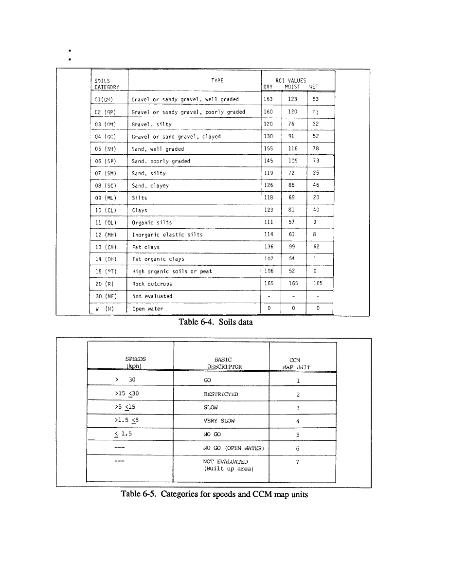
PART THREE
Synthesis Procedures
FM 5-33
Table 6-4, Soils data.
Table 6-5, Categories for speeds and CCM map units.
6-3

FM 5-33
Synthesis Procedure
PART THREE
Table 6-6, Vegetation factor data.
Table 6-7, Speed Prediction tabulation sheet.
Step 2.
Determine the vehicle to be used and whether the CCM product will be
prepared for dry or wet conditions or both.
Step 3.
Procure the surface configuration factor overlay and Tables 6-1 and 6-2.
Step 4.
Compute the F
1
speed/slope factor. This calculation determines the
extent that any slope will deteriorate the speed of the vehicle without consideration
for any other physical factor.
Using Table 6-1, determine the maximum off-road gradability (kph), maximum
on-road gradability (%), and maximum road speed (kph). Record this information
in the appropriate column of Table 6-2.
6-4
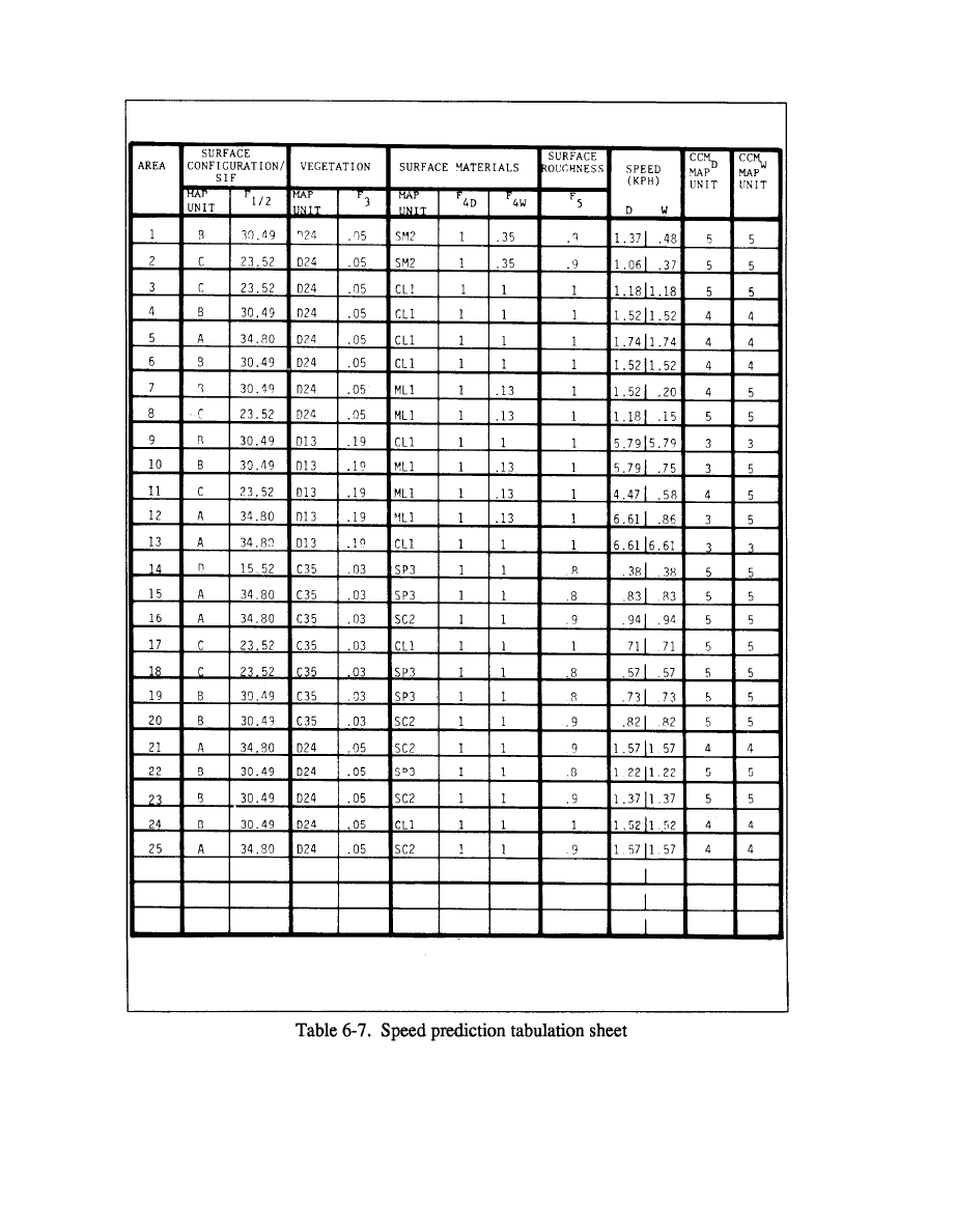
PART THREE
Synthesis Procedures
FM 5-33
6-5

FM 5-33
Synthesis Procedure
PART THREE
From the surface-configuration overlay, determine the percent of ground slope
for slope categories A through F. Use the mid-point value of the slope category as
ground slope, as shown below.
Example: Slope category = 10 to 20%
Ground slope = 15%
Record values of ground slope in the appropriate columns of Table 6-2.
Calculate F
1
values for each slope category.
a. Negative values indicate No-Go areas, use F
1
= 0.
b. Round values to nearest hundredth, then post them on Table 6-2.
Note: Rounding is critical to the final value.
c. F
1
for map unit G (naturally or culturally dissected terrain) represents an
unusual case and is best represented by using the lowest F
1
value obtained that still
permits movement.
Example: Calculate the slope category for the M113 (see Table 6-1).
Maximum off-road gradability = 45%
Maximum on-road gradability = 60%
Maximum road speed
= 48 kph
Ground slope
= 15% (midpoint of 10-20%)
F
1
= 24.0 kph
d. Record F
1
6-6
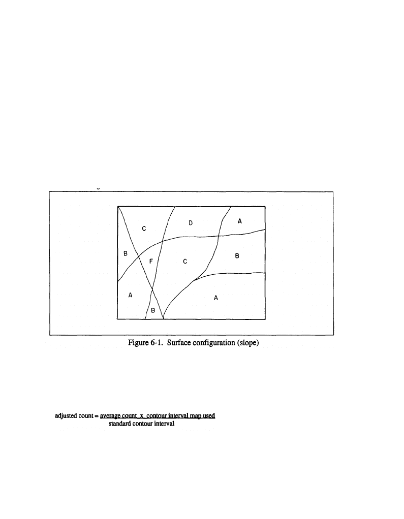
PART THREE
Synthesis Procedures
FM 5-33
Step 5.
Calculate F
2
, slope-intercept-frequency (SIF) factor. SIF is the number
of times the ground surface changes between positive and negative slopes over a
one-kilometer distance. Measuring this is extremely time-consuming in the field,
so use the expedient method.
a. Register the surface-configuration overlay to the appropriate topographic
map. In a slope category on the overlay, lay a line equal to the length of a diagonal
of a one-kilometer square (approximately l.4 times the length of 1 kilometer on
the map).
b. Count the number of times any contour line within the slope category crosses
or touches the diagonal.
c. Lay out a second line at right angles and count intercepts as before.
Note: A prepared template will greatly speed this operation.
d. Repeat this procedure at least ten times for each slope map unit, then average
the counts. See Figure 6-1.
e. Repeat this procedure for all slope categories A through F.
f. Adjust the average counts to the standard 1:50,000-scale map with a 20-meter
contour interval.
1) Determine the adjusted count, using the formula--
Example:
Contour interval of map used = 10 m
6-7

FM 5-33
Synthesis Procedure
PART THREE
Average SIP count
= 24.4
Standard contour interval = 20 m
= 12.2 (Round to 12 or the nearest
whole number).
2) Compute F
2
values for each slope category, using the formula--
Example: SIP = 12
3)
4)
F
2
= .96
Round values to the nearest hundredth, and record them on Table 6-2.
Record the lowest F
2
value on map unit G.
Step 6.
Calculate F, slope/SIF - speed calculation. This calculation gives the
calculated speed based on the effects and variation of slope.
a. Compute F values using the formula
F = F
1
x F
2
.
Example: F
1/2
= F
1
x F
2
F
1/2
= 24.0 kph x .96
F
1/2
= 23.04 kph
b. Record F in the appropriate column of Table 6-2.
Note: The value F will tell you what effect slope will have on vehicle speed.
Step 7.
Obtain F
3
vegetation factor.
a. Procure the vegetation-factor overlay and vegetation-roughness tables, Tables
1 and 6. Continuing with the previously selected vehicle, compute the F
3
vegeta-
tion factor.
b. Using Table 6-1, determine the vehicle width in meters (m), maximum
override diameter (m), and minimum turning radius (m) and record them on Table
6-8
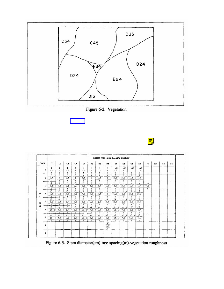
PART THREE
Synthesis Procedures
FM 5-33
c. From the vegetation factor overlay, determine the forest types and list them in
alphanumerical sequence on Table 6-6. List all other vegetation after the forest
types. See Figure 6-2.
d. From the vegetation roughness table on the vegetation-factor overlay, deter-
mine the stem diameter (m), stem spacings (m), and vegetation-roughness factor
for the appropriate forest types and record the information on Figure 6-6. See
Figure 6-3.
6-9
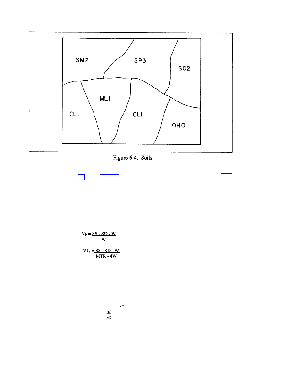
FM 5-33
Synthesis Procedure
PART THREE
e. For nonforest types, place the vegetation roughness factor in the appropriate
location on Table 6-2. For all forested areas, calculate V
1
1
is the product of the vehicle factor (VF) and the vehicle clearance factor
(V
1a
). VF accounts for the response of drivers when approaching wooded areas.
V
1a
accounts for the physical ability of a vehicle to maneuver between tree stems
in a wooded area.
Formula:
V
1
= (V
F
)(V
1a
)
Where--
SS = Stem Spacing (m)
SD = Stem Diameter (m)
W = Vehicle Width (m)
MTR = Minimum turning radius (m)
Notes:
1. if VF or V1a
2. if VF
3. if V
la
6-10
0, V
1a
= 0
1, V
F
= 1
1, V
1a
= 1.
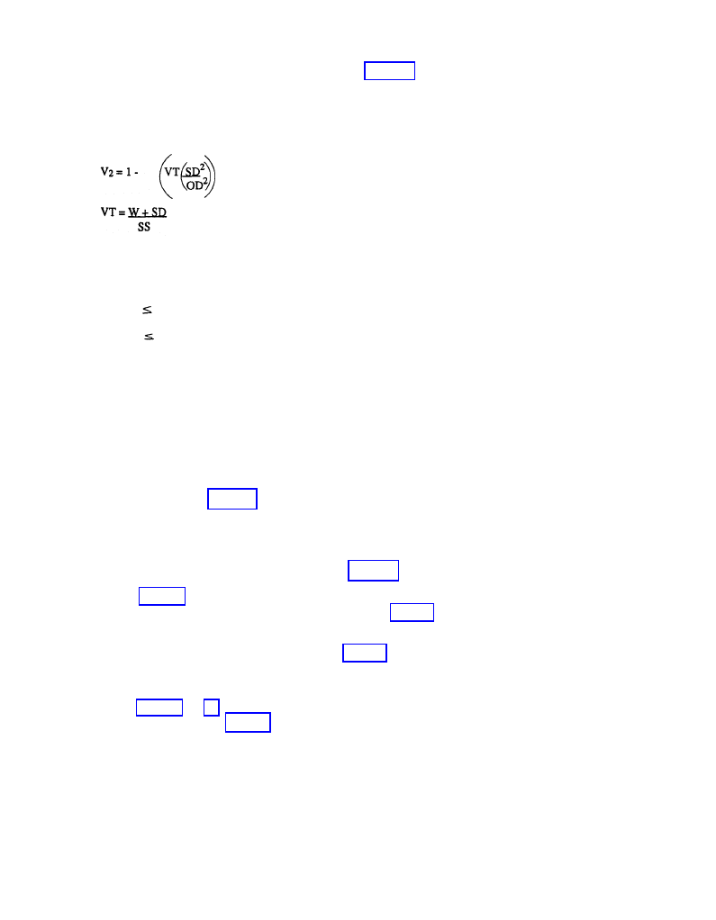
PART THREE
Synthesis Procedures
FM 5-33
f. Calculate V
2
for all forested areas and record it on Table 6-6. V
2
is the
calculation used to determine if it would be easier for the vehicle to override the
trees rather than maneuver between them. The VT portion of the formula is used
to calculate the minimum number of trees a vehicle can hit at one time.
Formula:
Notes:
1.
2.
3.
g.
if SD > OD, V
2
= 0.
if V
2
if VT
Calculate F
3
= Select the larger value between V
1
and V
2
.
0, V2 = 0.
1, VT = 1.
Formula: F3 = (VR)(V
1
or V
2
)
V
R
= vegetation roughness factor (obtain from the vegetation overlay)
Notes:
1. If F
3
> 1.0, F
3
= 1.0
2. If F
3
>0, F
3
= 0 (No-Go)
h. Record F
3
Step 8.
Procure the soil factor overlay and Tables 1, 3, and 4. Continuing with
the previously selected vehicle, compute the F
4
soil factor. This calculation will
determine if a particular soil type will support vehicular movement and to what
extent the speed will decrease due to that soil type. See Figure 6-4.
a. Using Table 6-1, determine the vehicle cone index (VCI
1
) for one pass and
the vehicle cone index (VCI
50
) for fifty passes. Record them on Table 6-3.
b. From the surface-materials factor overlay, extract the appropriate soils map
units, such as ML1, SM2, and OH0, and post them on Table 6-3.
Note: The third digit refers to the surface-roughness code.
c. From Tables 6-1 and 6-4, determine appropriate RCI values for dry and/or wet
conditions and post them on Table 6-3.
d. Calculate the dry-soil factor (F
4D
) and/or wet-soil factor (F
4W
) for each soil
type.
6-11

FM 5-33
Synthesis Procedure
PART THREE
Notes:
1. if F
4
2. if F
4
0, F
4
= 0 (No Go)
1, F4 = 1
e. Record F
4
CONSTRUCT COMPLEX FACTOR OVERLAY
Step 1.
Register the overlay to the base map.
Step 2.
Outline the built-up areas (color in red).
Step 3.
Outline the open-water areas (color in blue).
Step
4. Using the surface-configuration overlay and the vegetation-factor data
table, register complex overlay to the factor overlay and outline the slope areas
(color No-Go areas in yellow).
Step 5.
Using the vegetation factor overlays and Table 6-3, vegetation factor
data, register the complex overlay and outline the vegetation areas (do not draw
lines through areas already colored). Color No-Go areas in yellow, and disregard
areas less than 250 x 250 meters at map scale (5mm for 1:50,000) or narrow areas
less than 100 meters in width at map scale (2mm for 1,50:000).
Step 6.
Using surface-materials factor overlay and Table 6-4, soil factor (dry and
wet data), follow the procedures in Step 5.
Step
7. Beginning in the upper left comer, number the noncolored areas from 1
through 99. If you have more than 99 areas, outline the first area of 99 and label
it as Sector A. Number remaining areas 1 through 99, as before, and label them as
Section B. Continue numbering areas and sectors as required.
Step
8. Annotate all sector and area numbers on Table 6-5.
Step 9.
Compute CCM speed.
a. Using the completed complex factor overlay and the surface-configuration
factor overlay, determine the appropriate map unit for each area and post it on Table
b. Determine the F
1/2
value for the map units from Table 6-2 and post it on Table
c. Using the complex factor overlay, the vegetation overlay, and Table 6-3,
determine the map units and F
3
values and post them on Table 6-5.
6-12
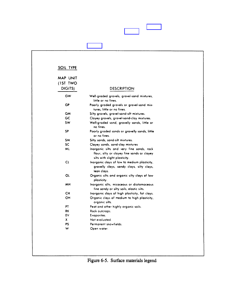
PART THREE
Synthesis Procedures
FM 5-33
d. Using the complex factor overlay, the surface materials overlay and Table 6-4,
determine the map units and F
4
values and post them on Table 6-5.
e. Determine the surface roughness factor (F
5
) for each area from the surface
materials overlay and post it on Table 6-5. See Figure 6-5.
6-13
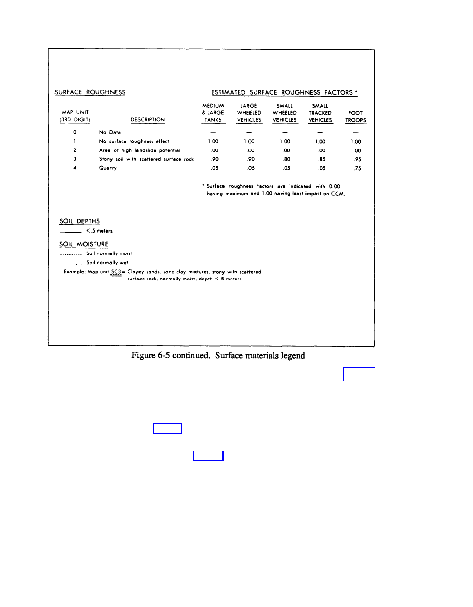
FM 5-33
Synthesis Procedure
PART THREE
f. Calculate the final CCM dry and/or wet speeds for each area. Use Table 6-7
and the following formula:
Speed (kph) = F1/2 x F
3
x F
4
W x F
5
Note: Round all interim and final calculations to the nearest hundredth. Post
g. Determine the CCM dry and/or wet map unit for each area using the CCM
legend, and post it on Table 6-5.
h. Combining areas of like CCM map units, draw the CCM product in final
format.
i. Add the appropriate linear obstacle data.
6-14

PART THREE
Synthesis Procedures
FM 5-33
PERFORM AVENUE OF APPROACH SYNTHESIS
PROCEDURE
An avenue of approach is a route that must offer some ease of movement plus
provide for an adequate dispersion of a friendly or enemy force large enough to
have a significant impact on a military operation. The avenue of approach product
does not include the status or possible actions of an enemy force. The end results
are avenues of approach suitable for friendly force configurations capable of
successfully completing the mission.
Step 1.
Combine and analyze previously completed terrain products such as the
CCM, transportation (LOC), and linear obstacle overlays and updated aerial
photography of the area of operations to produce mobility corridors.
Step 2.
Incorporate the limitations imposed by the battlefield terrain on friendly
and enemy doctrine.
Step 3.
Forward the data gathered in Steps 1 and 2 to G2 or S2 military
intelligence (MI) personnel to identify the terrain influence on the configuration of
friendly and enemy forces in the area of operations. MI personnel will evaluate
mobility corridors using the doctrinal template, which considers battle doctrine,
the tactical situation, and possible high-value targets.
6-15

PART THREE
Sythesis Procedures
FM 5-33
Line of Site and Zone of Entry
Chapter 7
LINE OF SITE
The line of site (LOS) is an unobstructed view from point A to point B. Requests
for LOS products are becoming more frequent just as the effective ranges of our
weapons, radar, and communications equipment are increasing. We can only
realize the effectiveness of long-range weapons with ranges of over 4,000 meters
and of current corps and division communications equipment with ranges of 50 to
60 kilometers if the equipment is emplaced properly in areas containing equivalent-
distance LOSs or groups of LOSs (as in fields of fire).
The seven methods for determining LOS are--
Ground truth (occupy positions), which is the most reliable, least likely,
and least convenient method.
Elevation layer tints, which do not consider refraction or the curvature of
the earth.
Survey intervisibility formula, which adds constants for curvature of the
earth and refraction but does not consider vegetation height.
Analytical Photogrammetric Positioning System (APPS), which is only
as good as equipment accessibility, operator training, and data-base ac-
curacy.
Profile (topographic map) method is the old, faithful method, almost
universally known, but which does not consider refraction or curvature of
the earth.
Aerial photography (the floating line method), which is better used for
short distances.
MICROFIX, which is accurate, dependent on access to digital terrain
elevation data (DTED), and useful for a wide variety of product.
As a terrain analyst, you must often determine if one location can be seen from
another location or if terrain is blocking the view. Intervisibility is the ability to
see from one object or station to another and is important to determine LOS. It can
7-1
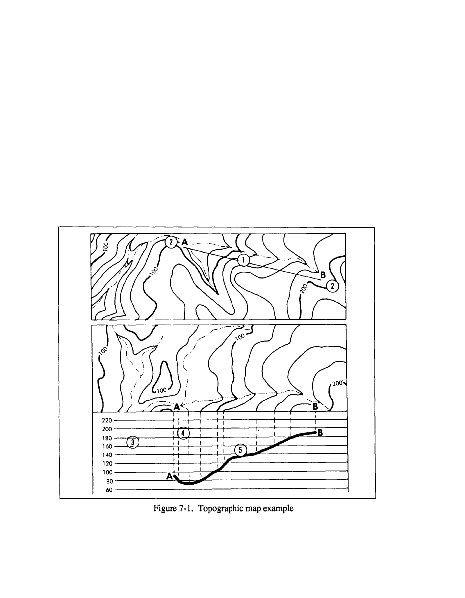
FM 5-33
Synthesis Procedures
PART THREE
be a tactical means of identifying defiladed areas for maneuver units or effects of
direct fire on ground forces. The best way to determine intervisibility is to
physically occupy each station. Since you cannot always be in the physical area,
however, you must use topographic maps and aerial photographs. You must be
able to plot coordinates on stereo-paired photos and construct a profile of a
topographic-map area.
Topographic Map Method
Make sure
you have your photo interpretation kit. It contains a photo plot, your
remote-sensed imagery (RSI), straightedge, pin vise and pin, point designation grid
(PDG) template, and a mission directive that contains location instructions.
Step 1.
Look at your mission directive to obtain information about the location
you will profile. The directive will also tell you which points to plot on the map.
Use the UTM coordinates on the map to plot the two points.
Step 2.
Draw a line across the area to be profiled connecting the two points you
have just plotted. This is the profile line. Figure 7-1 shows an example.
7-2

PART THREE
Synthesis Procedures
FM 6-33
Step 3.
Increase the value of the highest contour line. This will become the
upper-line measurement on the numbered profile lines. Start by looking at the map
and identifying the highest contour line that either crosses or touches the profile
line you have just drawn. Next, look at the bottom of your map and identify the
contour interval; for example, it may say “contour interval 20 meters.” Increase
the highest contour line by the contour interval. For example:
Highest contour line = 200 meters
Contour interval = 20 meters
200 + 20 = 220 meters
Step 4.
Decrease the value of the lowest contour line that touches or crosses the
profile line. This will become the lowest line measurement on the numbered profile
lines. Again, use the contour interval from the map. Decrease the lowest contour
line by the contour interval. For example:
Lowest contour line = 80 meters
Contour interval = 20 meters
80 - 20 = 60 meters
Step 5.
Prepare a profile. A profile is a side view of terrain along a line between
two points. On a blank sheet of paper, draw a straight line the same length as the
profile line paper. Each line represents a contour value line that crosses or touches
the parallel line. The highest elevation is at the top, the lowest is at the bottom.
Draw two additional lines at the top and bottom so that one line is above the highest
elevation and the other is below the lowest elevation. Number all lines to the right
or left in sequence, with the highest value at the top. The dotted lines at 220 and
60 are the two added lines.
Next, place your lined sheet of paper against the profile line on the map. Extend
dotted, vertical (perpendicular) lines from every point on the profile line to the
corresponding value line. Place a tick mark where each perpendicular line crosses
the profile line. This will ensure the contour value for each profile below a map.
Look at the perpendicular extensions from the contour lines to the corresponding
value line.
Step 6.
Interpolate hill and valley lines. Interpolation is a method of determining
the highest elevation of a hill and the lowest point of a valley. Since they are either
higher or lower than the known elevations, determine them separately. On the
profile, insert the interpolated lines between the other contour-value lines.
To estimate the height of a hill using the interpolation method, add half the contour
interval to the known elevation. For example:
Known elevation = 200 meters
Contour interval = 20 meters
1/2 Contour interval = 10 meters
200 + 10 = 210 meters
Interpolated value = 210 meters
To estimate the bottom of a valley using the interpolation method, subtract half
the contour interval from the known elevation. For example:
7-3

FM 5-33
Synthesis Procedures
PART THREE
Known elevation = 80 meters
Contour interval = 20 meters
1/2 Contour interval = 10 meters
80 - 10 = 70 meters
Interpolated value = 70 meters
Step 7.
Draw interpolated perpendicular lines extending to the corresponding
value lines. Notice how close they are to the highest and lowest elevation lines.
Step 8. Draw
a dark line connecting the perpendicular lines. Smooth, natural
lines represent hills and valleys. V- or U-shaped lines represent streams. Figure
7-1 illustrates a completed profile.
Aerial Photography Method
Step 1.
Orient the aerial photos for stereo viewing. Ensure that shadows of
features such as bridges, riverbanks, and low buildings appear to fall toward you,
the viewer.
Step 2.
Locate the PDG coordinates on each photo. PDG coordinates provide a
means of locating (plotting) points that represent features, targets, and positions on
an aerial photograph. Look in your mission directive to identify the PDG coor-
dinates of two points for each photograph. Place a grid over each photo, beginning
with the left one, and locate the grid square containing the point you will plot.
Using the standard “read right and up,” plot each point according to its PDG
coordinates. Use the standard map scale of 1:25,000, so you can use a map
protractor for plotting. Plot the points in order of the first point on the left photo,
first point on the right photo, second point on the left photo, and second point on
the right photo. Finally, enter the coordinates in the marginal information area on
each photo.
Step 3.
Pinprick the points on the photos, in the same order as in step 2.
Step 4.
Draw a connecting line between the points you have pin pricked and
connect points 1 and 3 on the left photograph. Next, connect points 2 and 4 on the
right photo. At this time, take a moment to cheek your work to make sure it is
accurate. The points you have plotted must correspond to the location in the
mission directive.
Step 5.
Place the stereoscope over the aerial photographs, with the left lens placed
over the left photo and the right lens over the right photo. Look through the
stereoscope and adjust the photographs slightly so you will get the best possible
stereo images. Features will appear to be three-dimensional if you have obtained
stereovision.
Step 6.
Determine intervisibility. After positioning the stereoscope over the
photos, look through your stereoscope. The two lines will fuse into one line. If it
appears to float above the ground, you have determined intervisibility. If the line
appears to cut through the ground, you have not. By determining intervisibility
between two points, you have also determined LOS between them.
7-4

PART THREE
Synthesis Procedures
FM 5-33
ZONE OF ENTRY
Categories
A zone of entry (ZOE) is any area in which forces, supplies, or equipment can
be placed within reach of an objective area. In most situations, it may also be a
zone of exit. Be prepared to show good exit zones from each ZOE, as exit zones
play a key role in the selection of ZOEs. Types of ZOEs are existing airfields, air
landing zones (ALZs), helicopter landing zones (HLZs), paratroop/resupply drop
zones (RDZs), ports, and amphibious landing beaches.
The three considerations of ZOEs are customers, terrain, and climate. Customer
consideration includes unit type and size, movement plans, and equipment type,
size, and loads. Terrain consideration includes vegetation, slope, surface materials,
obstacles, and surface drainage. Climatic considerations include temperature, air
density, air pressure, wind, speed, and visibility. See Figure 7-2 for potential
obstacles.
Airfields
Description
You can select existing airfields as potential ZOEs if they meet the minimum size
requirement dependent on the type of aircraft to be used. The easiest way to show
an existing airfield on a ZOE overlay is to use the same symbol that is used on the
transportation overlay, so the customer will know the runway length, width,
orientation, and pavement status.
Criteria
Airfields should accommodate the maximum size aircraft, have airfield facilities,
and be in correct orientation to the map scale. See Chapter 2 for information
concerning the elements of an airfield. See Figures 7-3, 7-4, 7-5.
7-5
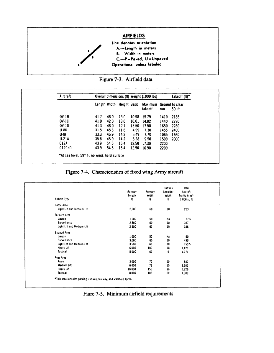
FM 5-33
Synthesis Procedures
PART THREE
7-6

Synthesis Procedures
FM 5-33
PART THREE
Air Landing Zones
Description
ALZs are entry zones used by fixed-wing aircraft to access objective areas. They
can include beaches, dry lake beds, sections of highway, and other areas that meet
the criteria. Areas are classified as hasty or deliberate based on the anticipated type
of missions or load requirements in a given area within the theater of operations.
Hasty ALZs are unimproved surfaces good only for marginal weather operations
and are unusable during prolonged periods of poor weather. Deliberate ALZs have
all-weather capability and are usually permanent installations with control towers,
runways, and taxiways. Deliberate classifications meet existing airfield criteria.
Figure 7-6 shows symbols for ALZ criteria. See TM 5-330 and FM 100-27 for
specific information.
Criteria
Undissected
% Slope - per 100-foot horizontal distance
No obstructions within glide angle of ALZ
Oriented with prevailing winds
Suitable Surface Materials and Surface Roughness
Procedures
Refer to FM 5-330 to determine proper values, then use the following formula
to compute ALZ length:
ALZ Length = TGR + ALT Cor + Temp Cor x SF + Slope Cor
Round Up.
Note: Round up the final ground run length to the next highest 100 foot value.
Example. ALZ length of 3,120 feet is rounded up to 3,200 feet.
Where:
TGR = Takeoff ground run at mean sea level and 59°F.
ALT Cor = Pressure altitude correction.
Add the dh value of entry zone based on FM 5-330 to the altitude of the entry
zone, then increase the TGR by 10 percent for each 1,000-foot increase in altitude.
Temp Cor =Temperature correction. If the corrected ground run obtained in the
previous computation is 5,000 feet or greater, increase the ground run by 7 percent
for each increase in temperature above 59°F; if less than 5,000 feet, increase
by 4 percent per 10° above 59°F. If the temperature is less than 59°F, no correction
is required.
7-7

FM 6-33
Synthesis Procedures
PART THREE
SF =Safety factor, Multiply the corrected ground run obtained in the previous
computation by 1.5 for rear- area ALZs and 1.25 for support, forward, and battle
area airfields.
Cor =Effective gradient correction. Increase the corrected ground run obtained
in the previous computation by 8 percent for each 1 percent of effective gradient
over 2 percent.
Round up =Round the final ground run length up to the next larger 100 feet.
Compare the final ALZ length and width to the minimum runway length and
width shown in TM 5-330 and use the larger of the two lengths and widths.
Helicopter Landing Zones (HLZs)
HLZs are entry zones in which helicopters access an objective area. They are
terrain and climate dependent. Even under the best weather conditions, using a
vertical approach and departure, the helicopter requires flat and obstacle-free open
areas and a surface material that will support the heavy loads of the aircraft. The
load factor, elevation, and air temperature determine whether the helicopter can
take off and land vertically. Helicopter approach and departure angles that are not
vertical require longer distances to clear obstacles surrounding the edges of the
entry zone.
Criteria
Undissected
Less than 15 percent slope (See FM 90-4)
Minimum size should be based on METT-T (20 - 75m guide, minimum
distance for a single helicopter)
No vertical or ground obstructions greater than or equal to 18 inches
10:1 obstacle clearance ratio
No dust, debris, or loose snow near LOC
Stable soils
Use the following formula to compute the size of the HLZ during daylight:
Where: LS = diameter of helicopter site
2 = safety factor
RTZ = radius of touch zone
HO = height of obstacle
DA = tangent of departure or approach angle in degrees, whichever
is smaller
Compare the final HLZ length and width to the minimum length and width shown
in FM 5-35. See Figures 7-8 and 7-9.
Use the following formula during hours of darkness:
LS (Daylight) x 1.43 = LS (Darkness)
7-8
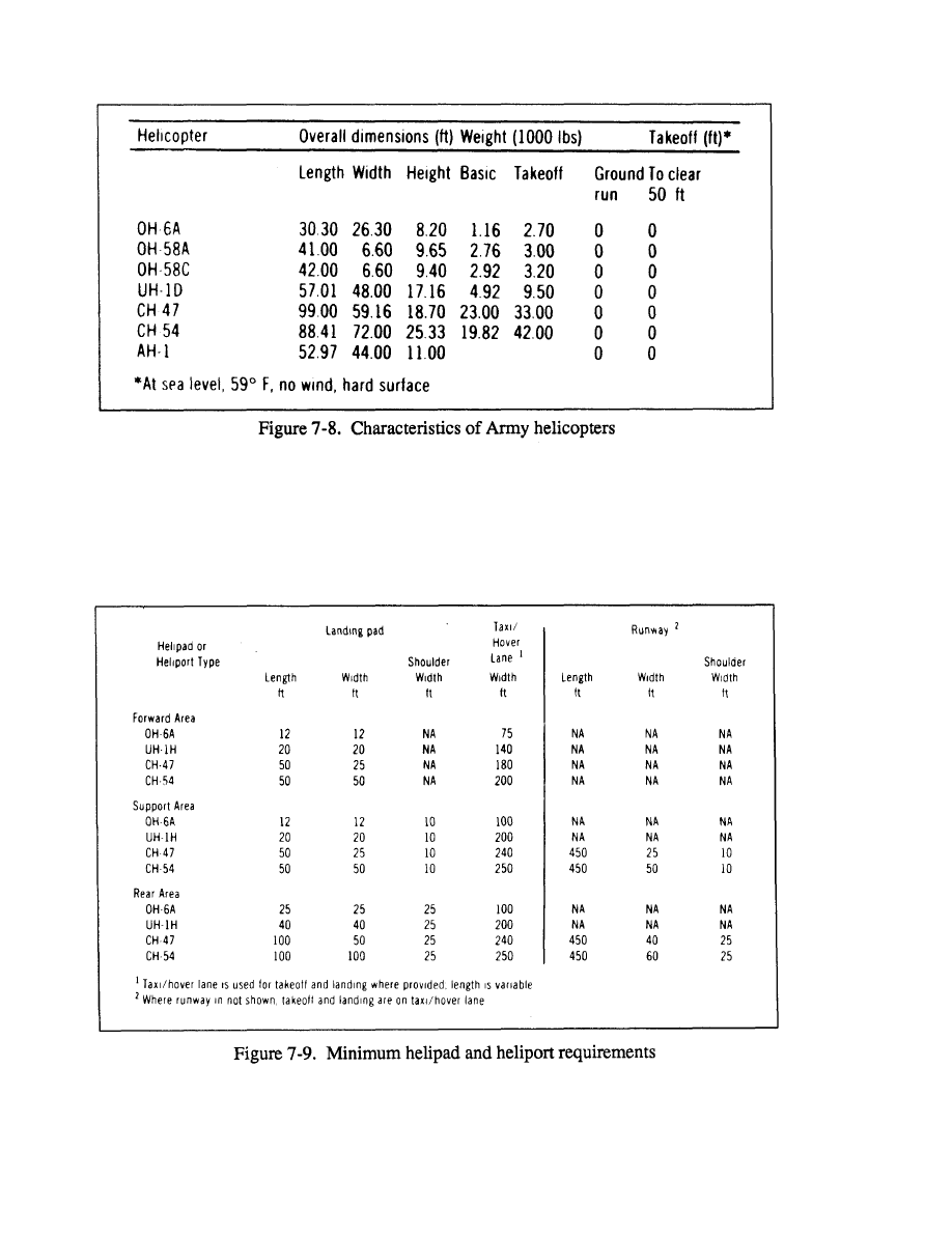
PART THREE
Synthesis Procedures
FM 5-33
Where: LS (Daylight)= Diameter of landing site during
daylight
1.43 = Safety factor for darkness
LS (Darkness)= Diameter of landing site
during darkness
Drop Zones (DZs)
7-9
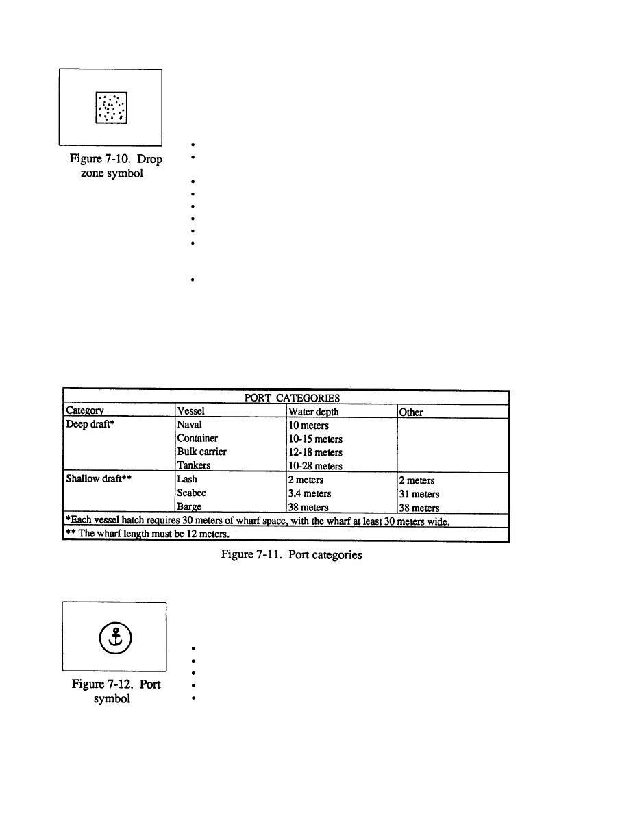
FM 5-33
Synthesis Procedures
PART THREE
DZs are entry zones in which troops or materials are delivered by parachute within
a close proximity of an objective area. They are sometimes called resupply drop
zones, when supplies are delivered to troops.
Criteria
Undissected
Less than 10 percent slope is preferred, 30 percent is allowable for supply
drops
Within 30km of a key city
DZ near LOC
No instructions within 1km
Must have routes of entry or exit
DZ has accessible cover and concealment
Minimum width and length is dependent on the type, formation and speed
of the aircraft, surface winds, the number of personnel or type of cargo
being dropped, and visibility.
For more information see FM 100-27.
Ports
Description
Ports may be used as entry zones when ships deliver troops and equipment close
to the objective area. The selection of a port as an entry zone is based on geographic
loceation, climatic conditions, and existing port facilities. Considerations include
basin protection, bottom condition, shore area, communications, and water depth.
Port categories are deep draft, which includes ocean-going vessels, and shallow
draft, which includes lighters, barges, and landing craft. See Figure 7-11.
Criteria
Water depth greater than 2 meters
Minimum length 30 meters per hatch
Exit route to Main Supply Route (MSR)
Near LOC
Near facilities
7-10

PART THREE
Synthesis Procedures
FM 5-33
DMA Pub 150 lists ports worldwide. See also FM 5-35.
Amphibious Landing Beaches
Amphibious landing beaches are entry zones in which troops and equipment are
involved in a transition from seaborne to a land attack force within a close proximity
to the objective area. The criteria used for determining the location of an am-
phibious landing zone is based on geographic and climatic conditions at the entry
zone. However, due to the transition from sea to land, the geographic conditions
are divided into two areas: conditions of the terrain at the entry zone and
hydrographic conditions at the entry zones. Additional considerations include
weather, extent, depth, and bottom of the sea area, beach approach, beach gradient,
and hinterland (depth, concealment and transportation net).
Criteria
Underwater gradient 30:1
Lack of underwater obstacles
Firm bottom
Trafficable soils exit
Tide information
Open, straight-shot of beach -no enemy salients
SYNTHESIS PROCEDURES
Step 1.
Review requirements to determine the type and criteria of the ZOE for
the projected area.
Step 2.
Obtain source material, including base topographic map, aerial photog-
raphy, and the vegetation, surface configuration, surface materials, obstacles,
surface drainage, and transportation factor overlays.
Step 3.
From the vegetation-factor overlay, extinct the following No-Go area:
All built-up areas
Vegetation categories A2, A3, Bl, B2, C1-C4, D1-D4, E1-E4, F, I, J, K,
L, M
Agriculture (A1) that includes bamboo, rice fields, and vineyards.
Step
4. From the surface-configuration-factor overlay extract the following
No-Go areas:
Any slope greater than 2 percent for ALZs
Any slope greater than 15 percent for HLZs
Any slope greater than 30 percent for DZs
Step 5.
From the surface-materials-factor overlay extract the following nonac-
ceptable soil types:
Permanent snowfields
Peat bogs
7-11

FM 5-33
Synthesis Procedures
PART THREE
Rock outcrops
Permanent wet soils
Surface roughness with a category of 3 or 4
Soil is probably not as important a factor as vegetation or slope. However,
powdery, dry soil in arid climates must be considered an impediment to helicopter
landing because of the reduced visibility, possible clogging of engine intakes, and
revealed helicopter location due to generation of dust plume. Very wet or mucky
soil may cause the helicopter wheels to settle into the soil to such an extent as to
prevent the accomplishment of the mission. Thus, soil conditions can be dangerous
to a helicopter and should always be considered when selecting a landing zone site.
Surface roughness affecting helicopter landing can include rocks, ridges, domes,
and sandbars. Skilled terrain analysts must determine surface roughness, visualiz-
ing the landform and making decisions concerning surface irregularities. For
example, some landforms of glacial origin commonly contain potential obstacles
such as boulders that are not mapped topographically and may be too small to be
seen on some aerial photography.
Step 6.
From the obstacle-factor overlay, extract all obstacles that are within the
project area.
The two types of obstacles associated with helicopter landing zone sites are
vertical obstacles, which affect helicopter approach to and departure from a landing
site, and ground obstacles within the landing site such as rocks, stumps, and holes.
Approach and departure obstacles include power lines, transmission towers, and
chimneys. These obstacles appear on standard 1:50,000-scale topographic maps
from which you can compile a factor overlay. Obstacles within the landing site
may not be detected easily. You must rely on ground reconnaissance, low-altitude
photography, or local geographic literature.
Step 7.
From the transportation-factor overlay, extract all existing airfields that
meet the criteria for ZOEs.
Step 8.
Evaluate all open areas and select the ZOEs needed for the projected area.
If available, evaluate the areas against the CCMs and LOCs of the area.
The criteria for minimum-size requirements depends on a number of factors,
including the type and number of aircraft, supplies, or troops to land in the ZOE,
temperature, wind, altitude, and geographic location. Therefore, use the criteria
listed for minimum areas as a guide and revise it as needed.
7-12
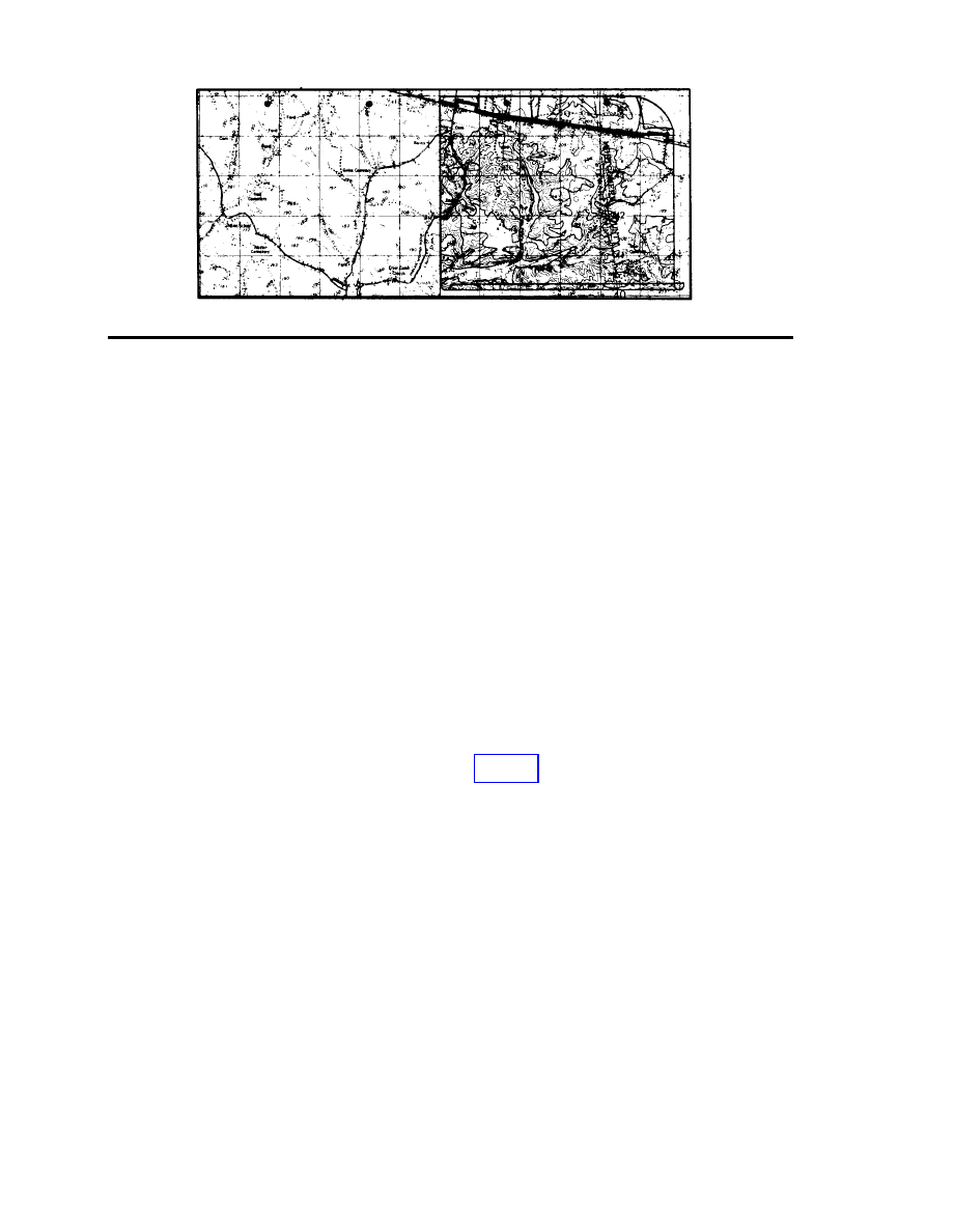
PART THREE
Synthesis Procedures
FM 5-33
Final Overlay Preparation
Chapter 8
After you have collected and processed the data, use the following steps to prepare
the final overlay:
Step 1.
Lay out the base map on a flat working surface, taping it on all four
corners.
Step 2.
Orient the working overlay to the base map. Check registration marks
on the draft overlay and line them up with the corners on the base map. Tape the
working overlay to the base map on all four corners.
Step 3.
Register the overlay material to the base map by tracing corner ticks from
base map onto the overlay material, using a fine point pen, so they form an L
approximately .5 inches by .5 inches.
Step 4.
Place the security classification at the top and bottom center of the
overlay.
Step 5.
Trace the outline of areas identified on the working overlay onto the final
overlay, and use the appropriate letters to correspond with the area. Do this with
each area to be outlined, until you have outlined all areas and depicted them with
the correct letters.
Step 6.
Step 7.
Step 8.
Step 9.
Place marginal data on the overlay according to Figure 8-1.
Construct a legend depicting all symbols used on the draft overlay.
Check the overlay for completeness, accuracy, and legibility.
Remove the overlay from the base.
Step 10.
Attach a classified cover sheet if it is required.
Step 11.
Deliver the overlay to your supervisor for review and storage.
8-1
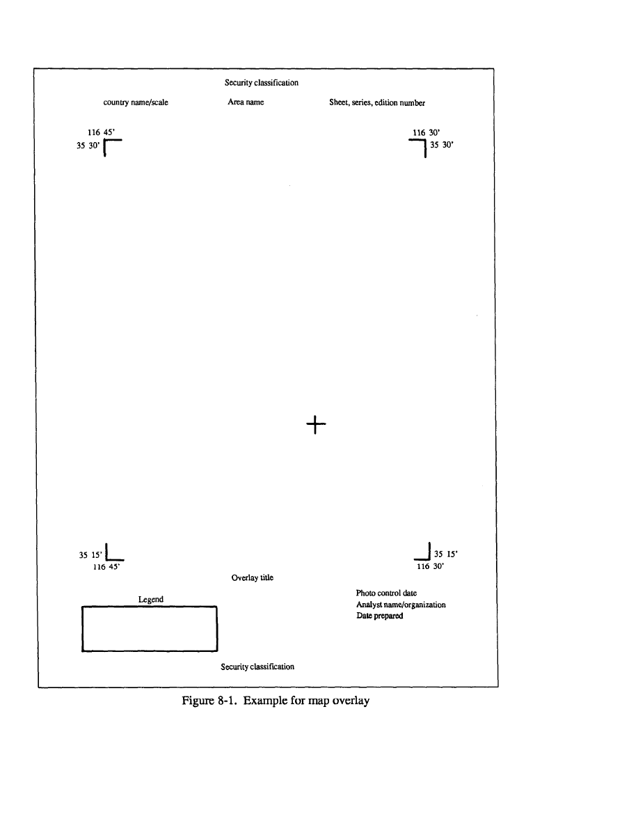
FM 5-33
Synthesis Procedures
PART THREE
8 - 2

PART FOUR
Formulas
FM 5-33
Vertical Photography
Chapter 9
Vertical photography is the process and the product of aerial photography taken
with the axis of the camera held in a truly vertical position. If the vertical
photography is taken over flat terrain, measured distances and directions may
approach the accuracy of a line on a map. Procedures for determining measure-
ments for vertical photography follow.
SCALE DETERMINATION
The linear scale is the relationship between distance on a map or photo and the
actual ground distance. Scale is expressed as a representative fraction (RF). RF
may be determined by one of three basic formulas:
Where--
RF=
f =
H=
h =
PD =
GD =
MD=
MSR =
The representative fraction or the scale of the imagery
The focal length of the camera
Height of aircraft above sea level
average terrain height above sea level
Photo distance on picture
Actual ground distance
Distance on map
Map scale reciprocal
Example: Find the RF of a photo where f equals 6 inches and H equals 5,000
feet.
GROUND DISTANCE DETERMINATION
You must know the photo representative fraction (PRF) or the map representative
fraction (MRF) to use the MSR or the PSR ground distance determination. To
9-1

FM 5-33
Formulas
PART FOUR
determine the actual distance or size of an object on an aerial photograph or map,
use one of two formulas:
GD = PD x PSR or GD = MD x MSR
Where--
GD =
PD =
MD=
PSR =
MSR =
Ground distance
Photo distance
Map distance
Photo scale reciprocal
Map scale reciprocal
Example Find the GD covered by a photo where the PD = 0.026 feet and
PRF = 1:8800.
GD = PD x PSR
GD = 0.026 feet x 8800 feet
GD = 228.8 feet
PLOTTING TEMPLATE ADJUSTMENT
The plotting template is an adjustable instrument used for plotting vertical aerial
photographs. The four sides of the template are graduated in inches and five
hundredths of inches and may readjusted to any combination of lengths and widths
from 0.05 inches by 0.05 inches to 5.0 inches by 5.0 inches. You can adjust the
template during inspection or with the formula--
Where--
TS = Template setting in inches
PS = Photo side (in inches)
PSR = Photo scale reciprocal
MSR = Map scale reciprocals
Example Find the TS of a photo where PS equals 9 inches by 9 inches,
PRF equals 1:5000, and MRF equals 1:25,000.
PROPORTIONAL DIVIDERS USE
The proportional divider is an adjustable, compass-like instrument designed
especially for enlarging or proportionally reducing drawings and sketches. Use the
formula---
Where--
scale ratio = Proportional divider setting
MSR = Map scale reciprocal
PSR = Photo scale reciprocal
Example Find the scale ratio when MRF equals 1:25,000 and PRF equals
1:5,000.
9-2

PART FOUR
Formulas
FM 5-33
PHOTO COVERAGE
Photo coverage is the ground area captured on any photo. It may be expressed
in square feet, square yards, or square miles. You can determine photo coverage
by using the formula--
Where--
PSC = PSR x PS
PSC = Photo side coverage on the ground
PSR = Photo scale reciprocal
PS = Photo side
Example Find the ground distance covered by each side of a photo with RF
equals 1:10,000 and photo format equals 9 inches by 9 inches.
PSC = PSR x PS
PSC = 10,000 x 9 inches
PSC = 10,000 x 0.75 feet
PSC = 7,500 feet
The total ground area covered by this photo is 7,500 feet by 7,500 feet or
56,250,000 square feet.
PHOTO COVERAGE FOR A SPECIFIC AREA
The photo coverage for a specific area refers to the number of photos required
to cover a predetermined area at a desired scale and format size. You must know--
The desired scale of the photography.
The photo format.
The size of the area to be covered.
The percentage of forward overlap between photos.
The percentage of side lap between flight lines.
Example Determine the number of photos required to cover an area 36,000
feet by 30,000 feet.
Where--
Photo format = 9 inches by 9 inches
Desired scale = 1:5,000
Forward overlap = 60 percent
Sidelap = 40 percent
Step 1.
Determine the ground-area coverage of a single photo.
Area coverage = format x PSR
Area coverage = .75 feet x 5,000
Area coverage = 3,750 feet x 3,750 feet
Step 2.
Determine the amount of ground gained forward (Ggf).
Ggf = Total area coverage minus forward overlap percentage
Ggf = 3,750 feet X 40%
Ggf = 1,500 feet
9-3

FM 5-33
Formulas
PART FOUR
Step 3.
Determine the amount of ground gained sideways (Ggs).
Ggs = Total area coverage minus sidelap
percentage
Ggs = 3,750 feet x 60%
Ggs = 2,250 feet
Step 4.
Determine the minimum number of photos per flight line.
Photo per flight line =
Photo per flight line =
Photo per flight line = 34
Step 5.
Round off photos per flight line to the next higher number when an uneven
number exists. Add two photos to each end of the flight line to ensure complete
stereo coverage.
Step 6.
Determine the number of flight lines.
Flight lines =
Flight lines =
Flight lines = 13 +
Step 7.
Round off the number of flight lines to next higher number when an
uneven number exists.
13+ = 14 flight lines
Step 8.
Multiply the number of photos per flight line by the number of flight lines
to get the total number of photos required to complete the mission.
14 x 38= 532 Photos required
HEIGHT DETERMINATION
Parallax Method
When you photograph a tall object from the air in two successive exposures,
the position of the point between the two photos appears to change. This displace
ment is called parallax, which you can measure to determine the height of an object
or the elevation of a point, using two overlapping vertical photos and taking
measurements in a prescribed manner. This is the most accurate method of
measuring height.
Step 1.
Attach the parallax bar to the cross member of the stereoscope legs with
the gage to the right. Push the ends of the bar down to engage the spring clips.
Slide the bar as close to you as the stereoscope legs will permit. This will place
the dots directly below the stereoscope lens. (See Figure 9-l.)
Step 2.
The stereometer is a stereoscope with special measuring attachments.
Under each lens is a glass plate that rests on its respective photograph of a
stereoscopic pair. On the bottom of each glass plate is a small dot. The dot under
the left lens remains in a fixed position. You can move the dot under the right lens
by an adjusting knob along the eye base of the stereometer. The movement of the
9-4
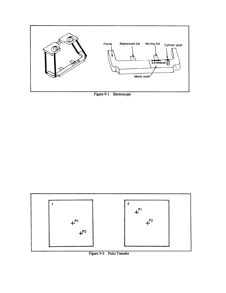
PART FOUR
Formulas
FM 5-33
right dot is measured by a micrometer dial. The range of distance between the dots
is significant. For example, when you turn the adjusting knob on a stereometer so
that the dots are at minimum separation, they may be 60 millimeters apart. When
you turn the adjusting knob so that the dots are at a maximum separation, they may
be 70 millimeters apart.
Corresponding points on two photographs must be between 60 and 70 millimeters
apart when the photographs are properly oriented for stereoscopic vision. Relative
to the graduation of the instrument the numbers may increase or decrease in
magnitude when the dots converge. For example, if there is a range of 10
millimeters between minimum and maximum separation of the dots, the readings
may be 0 at minimum and 10 at maximum or 0 at maximum and 10 at minimum,
depending on the type of stereometer.
Step 3.
Use fiducial marks to locate and mark principal points of both stereo
paired photographs. Both photos have their own principal points but also contain
the principal point of the adjacent photo in the aircraft flight line. To locate these
points, transfer them from one adjacent photo to another with a stereoscope. Orient
the photos for stereo viewing, locate the marked principal point, and mark the same
point on the adjacent photograph. Repeat this procedure with the other photo. Each
photo now has a principal point and a transferred principal point (see Figure 9-2).
9-5
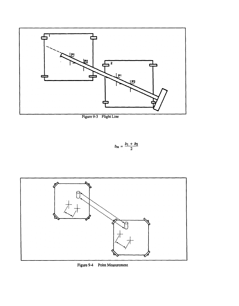
FM 5-33
Formulas
PART FOUR
Now you can establish the flight line by drawing a line from the principal point
to the transferred principal point on each photograph (see Figure 9-3).
Measure the distance from the principal point to the transferred principal point
(see Figure 9-4). Average these measurements using the formula--
Where--
b
m
= base means
b
l
= measurement from the principal point to the transferred
principal point on photo #l
b
2
= measurement from the principal point to the transferred
principal point on photo #2
9-6

PART FOUR
Formulas
FM 5-33
Step 4.
Locate the feature that you will measure using the stereoscope and
stereometer. Measure the top of the feature frost to obtain the first parallax
measurement p
1
. Then measure the bottom of the feature to obtain the second
parallax measurement, p
2
. To obtain a parallax measurement, you must place the
photos so you can see them in stereo. With the stereometer attached to the
stereoscope, you can see a left and right dot through the eyepieces. Place the left
dot on the point to be measured, then rotate the micrometer knob until the right dot
fuses with the left dot. Record the micrometer reading as shown on the scale.
After you have taken both parallax measurements (p
1
and p
2
), find the differential
parallax (
∆
p) to help determine the height of the feature, using the equation below.
You can use p, as a function of the elevation of the feature being measured, to
calculate the height of any natural or manmade object.
∆
p = p
l
-p
2
Step 5.
Since all elevations are relative to each other, you must establish a
reference elevation to measure height differences. This reference elevation is the
average terrain elevation above mean sea level, the horizontal plane above which
an aircraft photographs. You can reference the terrain elevation of certain objects
shown on aerial photography from topographic maps of the same area. This data
can be used to provide an estimation of the average terrain elevation (h). For
parallax height determination, you must also know the altitude of the aircraft, which
you can determine from the marginal information on the aerial photograph. The
altitude shown on the photo is the aircraft height above mean sea level (H).
Step 6.
Once you have taken all measurements from the stereo-paired
photographs, you can use the parallax equation to solve height determination, as
follows:
Example:
a. Determine the base means.
b. Determine the differential parallax.
∆
p = p
1
-p
2
∆
p = .0435 feet - .0410 feet = .0025 feet
c. Determine height.
Height =
Height =
Height =
Height =
Height =
9-7
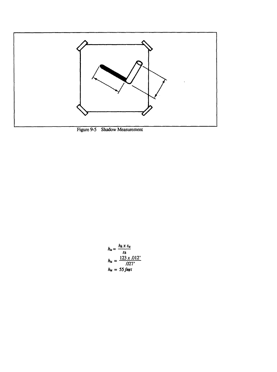
FM 5-33
Formulas
PART FOUR
Shadow Method
The shadow method is the least accurate of the three methods. You must have
an object with a known height, and the unknown object must cast a shadow onto
flat ground (see Figure 9-5). If the ground is uneven, the answer will be inaccurate.
For any relatively small area of level ground, shadow length is directly proportional
to object height. For example, a 40-foot tower casts a shadow twice as long as a
20-foot tower. If the shadow lengths are in a certain ratio, their photo images will
be in the same ratio. To determine the height of an unknown object, measure its
shadow length and multiply it by the ratio of height to shadow length established
from the known object. Using the microcomparator or the photo interpreter’s scale,
measure the height of the unknown object and its shadow length. Place those
measurements into the equation and determine the height using the following
formula
Example:
h
k
= 123 feet
s
k
= .027 feet
s
u
= .012 feet
Where--
h
u
= height of unknown object
k = height of known object
Su = shadow length of unknown object
S
k
= shadow length of known object
9-8
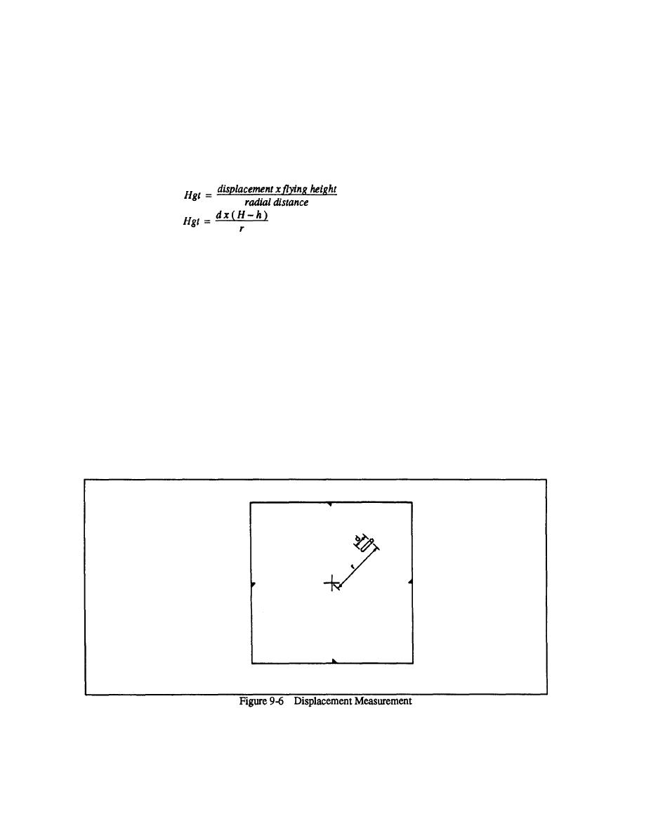
PART FOUR
Formulas
FM 5-33
Relief Displacement Method
The determination of height from relief displacement employs a single, vertical
aerial photograph where both the base and the top of a vertical object are
measurable. This method is particularly effective on large-scale imagery. For it
to work, the displacement of the image must be visible. The formula for determin-
ing the height of an object based on its relief displacement is--
Hgt =
H =
h =
H-h =
d =
r =
Height of the object above the average terrain
elevation
Altitude of the aircraft above mean sea level
Average terrain height above mean sea level
Altitude above ground level
Image distance representing vertical side of the object
Distance between principal point and top of the object
scaled from the photograph
You will first need to use a straightedge and mark the center of the photograph
with fiducial marks. Always measure r from the top of the object to the center of
the photograph, which you must determine by the intersection of the lines connect-
ing the opposite fiducial marks. Measure d between the same point on the top and
on the bottom of the object. The top of the object is always farther away from the
center of the photograph than the bottom (see Figure 9-6). Using the photo-
interpreter’s scale, measure the distances and place the numbers into the equation,
using procedures discussed earlier.
9-9

FM 5-33
Example
Formulas
PART FOUR
AREA MEASUREMENT
You can use the dot grid template to measure area. Randomly place it on the lake
or area to be measured. Count the dots that fall within the lake and those that fall
on the line. Record the number, repeat the procedure at least three times, and
determine the mean number of dots by adding the numbers together and dividing
by the number of counts.
Example
First count
= 13
Second count
= 12
Third count
= 12
13+12+12
= 37
37/3
= 12.3
Mean number of dots
= 12.3
Step 1.
Calculate the area in cm using the formula:
Example:
cm
2
= .49 cm
2
Note: Dots per cm
2
in this example are 25. Other dot grids are available, so
check in each case to determine the dots per cm
2
.
Step 2.
Calculate the ground area using the formula--
Area = object area in cm
2
x DRF
2
Example:
DRF = 24,000
DRF
2
= 5.76x10
8
Area = (.49cm
2)
x (5.76 x 10
8
)
Area = 2.8224 x 10
8
cm
2
Where-- DRF = the denominator of the map or photo RF
Step 3.
Convert the answer you obtained in Step 2 to square meters, using the
formula--
m
2
= cm
2
x .0001
m
2
= (2.8224 x 10
8
cm
2
) x (.0001)
m
2
= 28,224
9-10
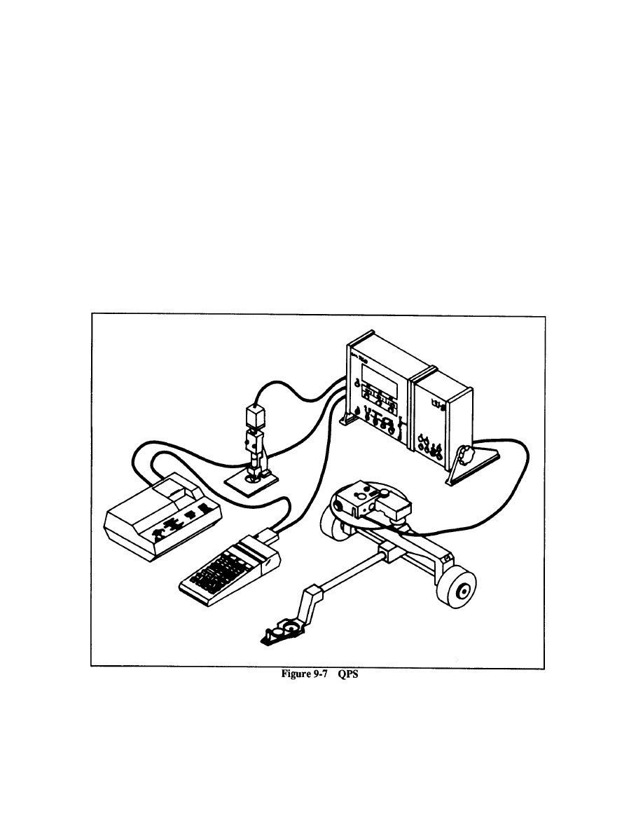
PART FOUR
Formulas
FM 5-33
Examples:
a. Calculate the volume of a lake which is 3 meters deep and has a surface of
28,800m
2
.
Volume = 28,800m
2
x 3m
Volume = 86,400m
3
b. Calculate the lake volume in gallons.
1 m
3
= 264.7 gallons of water
Number of gallons = (264.7 gallons/m
2
) x (86,400m
3
)
Number of gallons = 22,870,080
QPS AREA MEASUREMENT
The QPS computes measurements automatically, greatly helping analysts find
surface areas and volumes (see Figure 9-7).
When the operator moves the QPS, it measures length, area, or volume. All
measurements are displayed in the proper scale and units, and analysts can print a
9-11

FM 5-33
Formulas
PART FOUR
hard copy of the measurement results on command or automatically. The QPS is
not affected by any detrimental physical condition of a map or photograph that is
to be measured, such as tears, wrinkles, or folds. QPS components include--
A calculator, which is capable of data storage and manipulation.
A point counter, which enables automatic determination of the
count total for specific features or items located on drawings,
maps, and so forth.
A planimeter, which estimates surface areas and volumes.
A linear measuring probe, which measures lines and distances.
See TM 5-6675-324-14, TM 5-6675-325-14, and TM 5-6675-326-14 for more
information on the QPS system. See Appendix C for sources of aerial and
ground imagery.
9-12
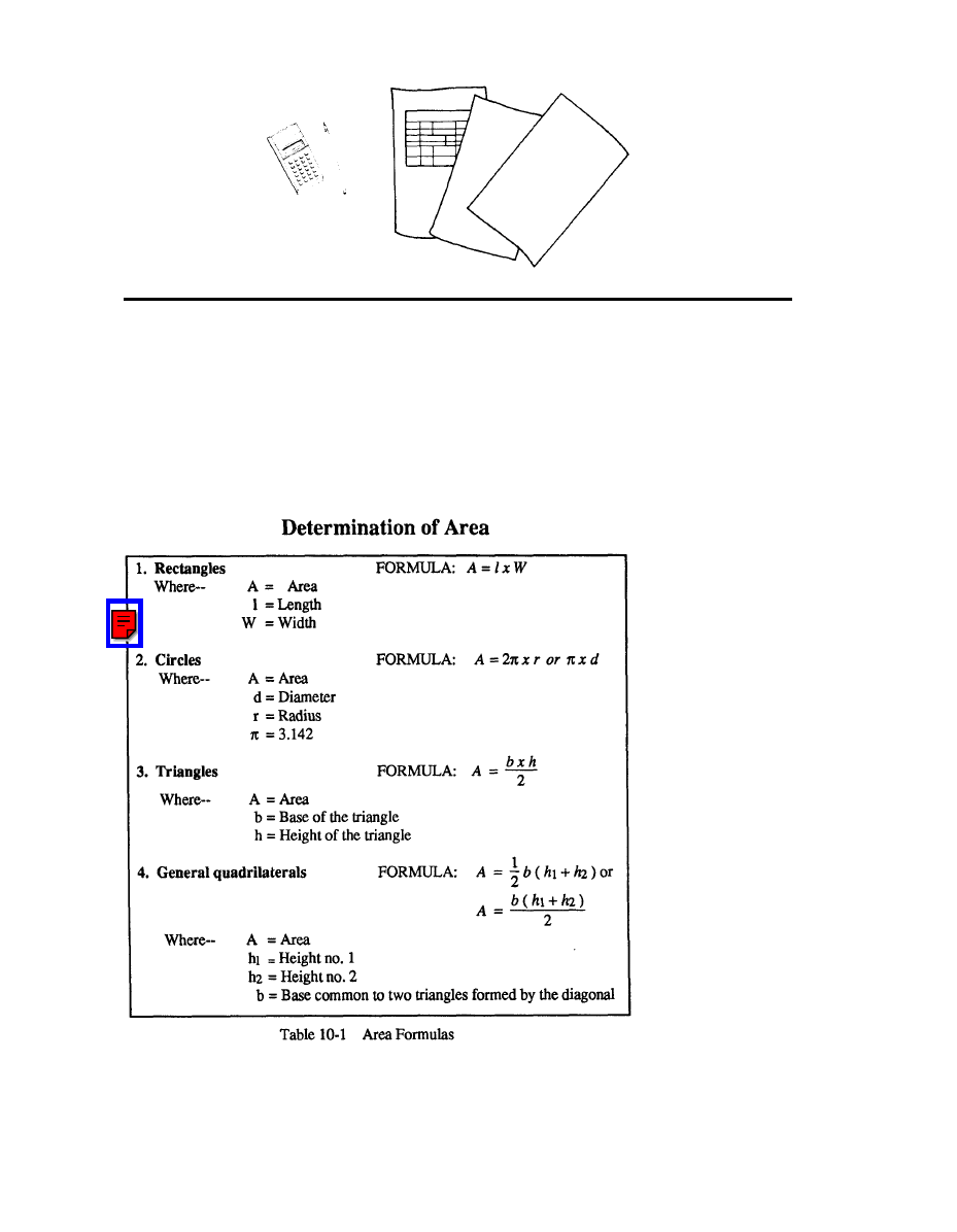
PART FOUR
Formulas
FM 5-33
Mathematical Techniques
Chapter 10
GEOMETRIC FUNCTIONS
The result of any operation performed by terrain analysts will only be as accurate
as the measurements used. An interpretation and detailed analysis often requires
terrain analysts to use basic geometric functions. In addition, approximation of
volume, extent of stock piles, and capacity of floor space require geometric
formulas. Therefore, analysts must have a sound background in the fundamentals
of basic imagery math. This section serves as a guide to a unique and comprehen-
sive collection of current geometric formulas that are basic to all types of imagery
interpretation.
10-1
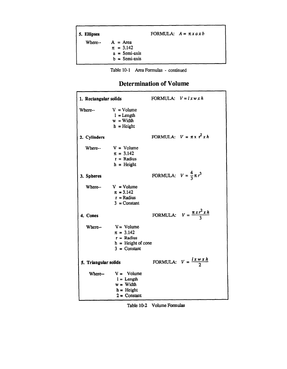
FM 5-33
Formulas
PART FOUR
10-2
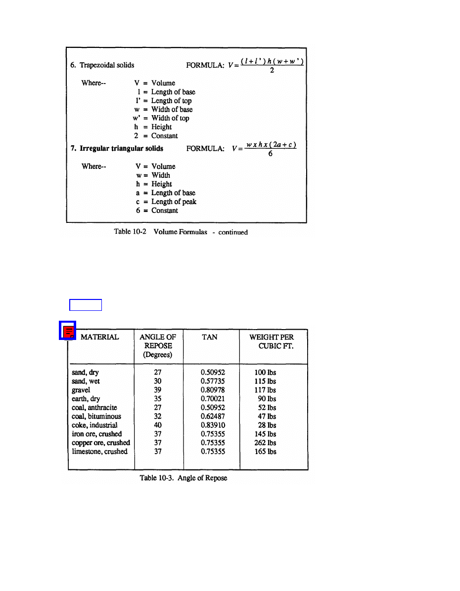
PART FOUR
Formulas
FM 5-33
Angle of Repose
The angle of repose of any material is the angle at which material will stand when
piled. Moisture content is often the controlling factor. The percent of fine material
in the mass has a decided influence on the angle, as the fine carries the bulk of the
moisture. Screened material has an angle of repose of 35 to 40 degrees.
Table 10-1 gives the average angle of repose and the average weight per cubic
foot of various materials of interest to the terrain analyst.
Thus, knowing the angle of repose of a specific material, we can solve for
height, using the horizontal dimensions.
10-3

FM 5-33
Formulas
PART FOUR
Example: Find the height (h) of a pile of limestone.
Formula:
h = 0.75355 x 20 ft.
h = 15.071 ft.
Where--
b = 40 feet
Angle A = 37 degrees
Tan 37° = 0.75355 (from Table 10-1)
TRIGONOMETRIC FUNCTIONS
Oblique photos and thermal and SLAR imagery are often used to supplement or
take the place of vertical photographs. In order to ensure maximum use of this
imagery, the interpreter must be familiar with certain concepts, formulas, and
principles concerning their accurate interpretation. This section gives the terrain
analyst a basic understanding of trigonometric functions necessary for solving
problems dealing with these special types of imagery, as well as a table of
trigonometric conversions.
Six Functions
To define the six trigonometric functions upon which trigonometry is based,
consider the angle, initial side AQ, and terminal side AS.
Choose any point B, different from A on the terminal side AS, and drop a
perpendicular BC to the initial side AQ. From the three sides (BC, AC, and AB)
associated with point B, six ratios are formed which are called the six trigonometric
functions of Q.
These ratios are independent of the position of the point B on the freed terminal
side AS, for if we choose any other point B1 on AS and drop the perpendicular
BlC1 to the initial side AQ, the two right triangles ABC and AB1C1 are similar.
Therefore, their corresponding sides have the same ratios.
If the angle is placed in standard position on a coordinate system, and the distance
AB is designated by c, the six trigonometric functions may be defined as follows:
10-4
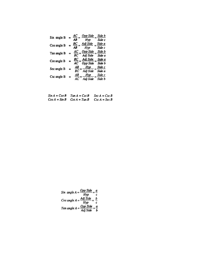
PART FOUR
Formulas
FM 5-33
To define trigonometric functions of the sides of right triangles, one will
often find it convenient to use the functions of an acute angle. Thus, functions
of the acute angle B may be written as follows:
By comparing the values of the functions of angle A and angle B, we find the
following equations:
Since angles A and B are complementary, the cosine, cotangent, and cosecant are
called cofunctions of the sine, tangent and secant respectively. Conversely, we
may state the following theorem: Any trigonometric function of an acute angle is
equal to the corresponding cofunction of its complementary angle.
We can use this theorem to express any function of an angle greater than 45
degrees in terms of a function of an angle less than 45 degrees. For this reason,
tables of values of the trigonometric functions need be computed only for angles
from 0 to 45 degrees instead of from 0 to 90 degrees.
Illustrations: (a) Sin 76°43’ = Cos 90° -76° 43’= Cos 13°17’
(b) Cot 51° 28’9“ = Tan 90° - 51°28’ 9“= Tan 38°31’51”
Right Triangles
Terrain analysts will use the functions of the right triangle most often for
interpretation purposes. In any triangle, the sum of the interior angles is 180
degrees. If the triangle to be solved is a right triangle, one of the known parts in
any case is the angle C; that is, C = 90 degrees, and A + B = 90 degrees. To solve
a right triangle, therefore, we must find two sides or one side and an acute angle,
using the formulas--
A + B =90 degrees
.
10-5

FM 5-33
Formulas
PART FOUR
If two sides are given, we can find the sin of angle A from the above formulas
involving the two given sides. We may then use another formula to find the
remaining side, and then find angle B by subtracting angle A from 90 degrees.
If one side of an acute angle is given, we begin by finding the other acute
angle. Then we select one of the trigonometric formulas containing an unknown
side and solve for it.
Pythagorean Theorem
The Pythagorean theorem provides a method for finding the lengths of the sides
of a right triangle and checking the trigonometric method, with the statement: The
square of the hypotenuse of a right triangle is equal to the sum of the squares of the
other two sides. Related to a right triangle labeled A, B, and C, as shown previously
and reproduced here for convenience, the theorem may be stated as the formula
a
2
+ b
2
= c
2
or
c
2
= a
2
+ b
2
Note: In order to solve the formula, we must understand the solution to the
square root function. The square root of a number is the result of a number
multiplied by itself. For example, 2 x 2 = 4, so the square root of 4 is 2.
10-6
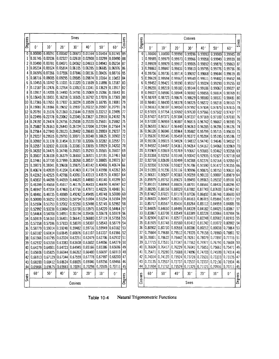
PART FOUR
Formulas
FM 5-33
10-7
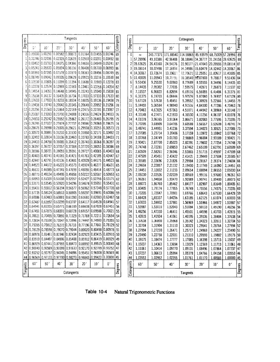
FM 5-33
Formulas
PART FOUR
10-8
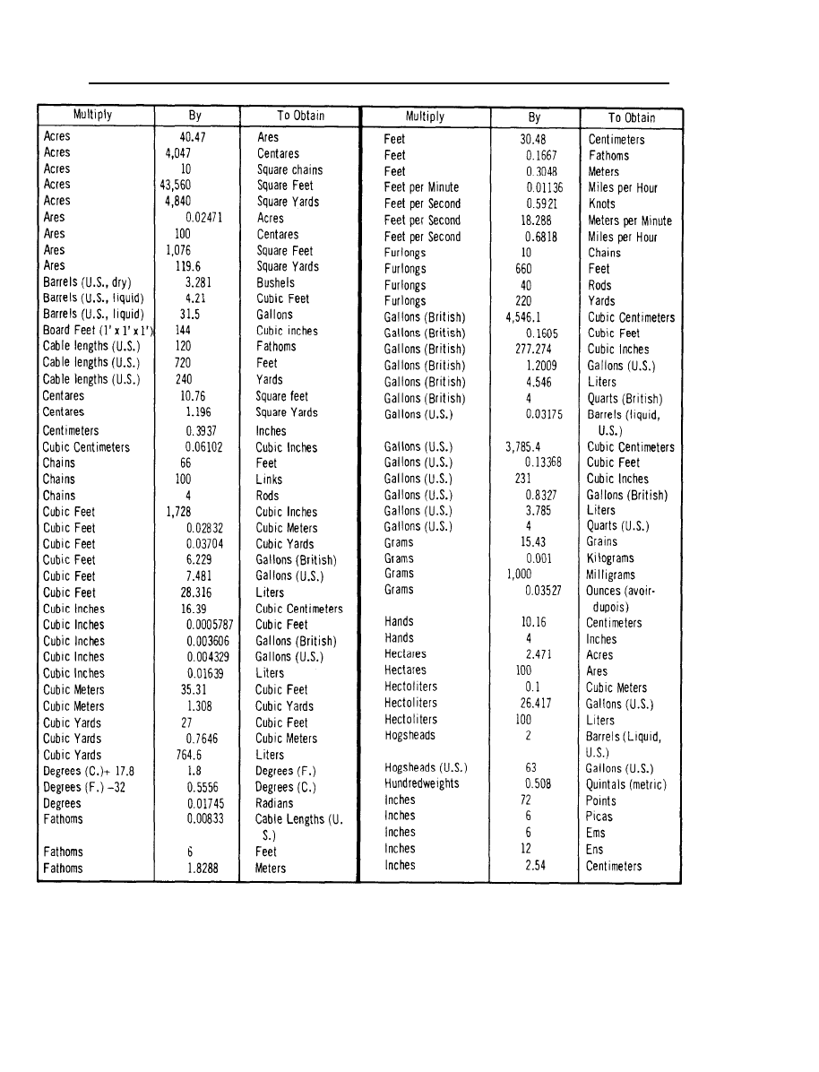
Mensural Conversions
Appendix A
A-1
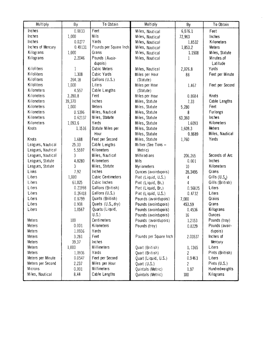
A-2

A-3

Weather
Appendix B
To understand the interactions between weather and terrain and to work effectively with the
staff weather officer (SWO), the terrain analyst must have a basic knowledge of weather
phenomena and weather support procedures. This appendix discusses weather and
weather-related factors that may affect military operations.
In addition to terrain, the battlefield environment includes atmosphere (weather),
battle-induced contaminants (man-made weather), background signatures, and illumination
(both natural and man-made). The terrain analyst, intelligence analyst, and United States Air
Force weather personnel work together to integrate these environmental factors with terrain to
determine their net effects on mobility and weapons usage. While weather effects on personnel
and tactics are specifically an intelligence function, the same environmental phenomena also
affect topographic engineer concerns. Therefore, analysis of factors should be a joint effort
between topographic engineer, intelligence, and USAF weather personnel. The analyst should
have a general knowledge of weather phenomena and its interaction with terrain. The analyst
should also know how to get and use weather information. Since equipment and procedures
change frequently, analysts should get specific information from the unit involved about
effects of the weather on unit equipment and operations.
TYPES OF WEATHER INFORMATION
The three groups of weather information are observations, forecasts, and climatology. Units
use observations and forecasts in support of current operations, while they use climatology for
long-range planning.
Weather Observations
Weather observations are reports of actual weather conditions existing at a specific location
at a given time. Observations are determined visually, with instruments, or both. Terrain
analysts will base much of their analysis on current weather observations, since weather
information can change very quickly. For this reason, units must also keep observations
current. The SWO generally receives weather observations in codes comprised of
abbreviations, numbers, letters, and symbols. Codes are used to simplify and speed
transmission, not because of classification. The USAF weather personnel can explain the
codes used in a given area.
The SWO can obtain observations taken by USAF weather observers, Army personnel in the
Forward Area Limited Observation Program (FALOP), artillery meteorology (ARTYMET), and
domestic and foreign weather services.
B-1

Unfortunately, weather observations are not always available, nor do they always contain the
weather parameters of interest. However, the weather forecaster can forecast the present
weather at a given location for which observations are not available. This forecast is called a
“nowcast”; the complexity of the meteorological situation and the forecaster’s knowledge of
past conditions at that location determine its accuracy.
Weather Forecasts
SWOs usually base weather support to current operations on observed current weather and
on weather forecasts. Weather forecasts are predictions of future weather for a specific period
at a specific location or area. Forecast accuracy depends on the time range being forecast, the
complexity of the meteorological situation, and the amount and quality of data available.
Forecasts for longer time ranges are more general in nature and less accurate than those for 24
hours or less. Forecasts longer than a week are rarely very accurate because of our limited
knowledge of how the weather operates. Thus, forecasters usually base long-range forecasts on
climatology, a statistical summary of usual weather conditions for a given location and time of
the year.
When possible, analysts should present observed weather along with forecast weather
information. This lends credence to the forecast and gives the commander a sense of the
reliability of the forecast. Weather forecasting is not an exact science, and not all forecasts
will be accurate. The SWO will be more confident in the forecast in some situations than in
others. Analysts should keep in contact with the SWO in case the forecast changes and should
check the progress of the weather observations for their area of operations.
Climatology
Climate refers to the characteristic weather for a given place or area over a specified time.
It is usually represented by statistics of weather conditions such as mean values, extreme
values, and probability distributions. Commanders use climatology for planning upcoming
operations. The SWO should have climatological information for the unit area. If not, he can
get it from higher USAF channels. If the unit does not have an SWO, analysts can order
climatology data directly from the Air Force under procedures in AR 115-1. Response time
depends on whether the data exists and whether it exists in the format needed. Often it will be
better to change the request so it can be filled with immediately available data than to demand
specific computer-formulated data, which could take more time to get.
Often information from standard climatological summaries will be satisfactory, and units can
get it quickly. Examples of such information include normal daily maximum and minimum
surface temperatures and normal monthly rainfall amounts. If the supported unit has specific
weather sensitivities not covered in standard climatological summaries, USAFETAC can
formulate statistics to meet those needs. For example, if a unit has a weapon system that is
limited by surface winds of 20 knots or more, the analyst can request statistics on the monthly
frequencies of such winds and statistics indicating how often particular hours of the day have
winds of 20 knots or more.
Two problems arise from using climatology. First, the specific information may not be
available.
Observations at that location may never have been taken, or the available
observations may not include the specific parameter. Consequently, there is no data base upon
which to formulate statistics. Units can usually overcome this shortage by the SWO or
USAFETAC estimating weather conditions from nearby stations for which data is available.
Second, too much data is sometimes available. This can create a difficult situation, in which
the analyst must be careful not to swamp a commander with useless statistics and unnecessary
B-2

detail. Thus, the analyst must know which weather conditions will affect the unit’s operations
and work with the SWO to present a concise summary of pertinent climatology.
WEATHER ELEMENTS
This section describes the application of the more common weather elements to terrain
analysis. It contains the basic knowledge needed to work effectively with WETM and
intelligence personnel. The information here is not complete; specific information about
weather effects on the equipment used by the supported unit must come from that unit itself.
Weather effects on terrain can be complex; unfortunately, few tactical decision aids are
available. Until further procedures are available, much of the application of weather
information will depend on the combined judgement and experience of the terrain analyst,
SWO, and intelligence analyst.
Temperature
Temperature, alone or in combination with other weather elements, impacts on many
actvities. Extremes of temperature are a discomfort to personnel and can affect equipment and
weapons systems. The difference between the temperature of a target and its background is
critical to weapons using infrared sighting devices. This section outlines some factors to
remember in using temperature information.
Surface temperatures in North America are generally measured in degrees Fahrenheit (
0
F);
elsewhere they are reported in degrees Celsius (
0
C).
Analysts always report upper air
temperatures in degrees Celsius. Conversion between the two temperature scales is by the
following formulas:
F=(9/5x C) +32
C=5/9x (F-32)
Temperature is normally measured at about 5 feet above a grassy surface, with the
thermometer shielded from direct sunlight and precipitation. This temperature is not
necessarily the same as the temperature just above the surface of the ground. The temperature
at grass level can be several degrees higher during the day and several degrees cooler at night.
Temperature is dependent on topography, with higher elevations generally being cooler,
However, since cold air is denser than warm air, cold air tends to flow into lower areas on
nights with light winds.
Analysts must remember that objects are not necessarily the same temperature as the air.
Metal objects exposed to sunlight, for example, tend to be hotter than air temperature, due to
their absorption of solar radiation. At night they tend to be cooler than the air, because they
lose their heat more rapidly by radiation. This can be very important to infrared sensing
devices.
Windchill equivalent temperature (WCET), often simply called wind chill, is an
approximation of the combined effect of temperature and wind on the exposed human body.
Analysts must remember that the air movement causing windchill comes not only from wind
but from any movement of the body relative to the air. Riding in an open truck moving at 20
mph in a 10-mph headwind gives a windchill equivalent to a 30 miles per hour wind.
Windchill does not apply to equipment. For example, with a -10° F temperature, a battery will
perform the same in calm conditions as in a 20-mph wind.
Frozen ground can be critical to trafficability. Frost depth depends on soil type, soil
moisture content, type of ground cover, and recent temperature history at the site. Given the
same soil and weather conditions, increased soil moisture (up to near the point of saturation)
B-3
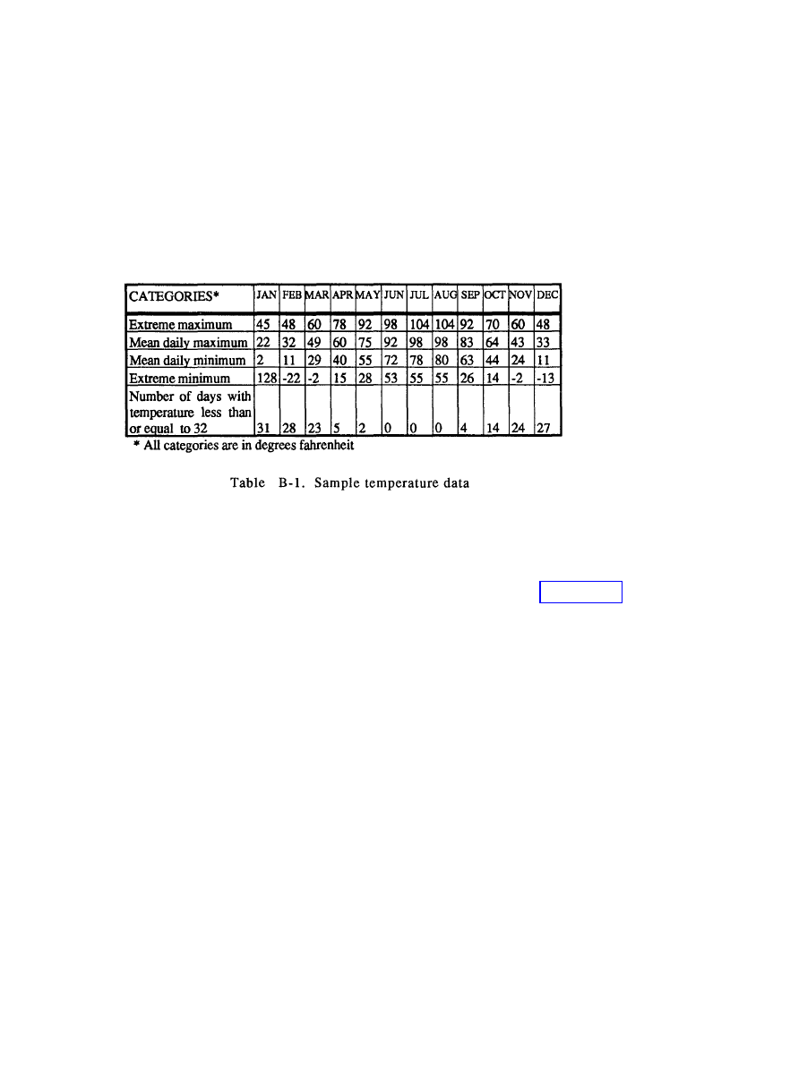
will cause frost to penetrate deeper and faster. Bare soil will normally also freeze faster and
deeper than sod-covered areas. Snow cover is an excellent insulator and can cause depth of
frost to be shallower than in areas without snow cover. Usually, few observations of frost
depth will be available. Furthermore, frost depth cannot be forecast now. Analysts will
probably have to depend on their own observations of frost depth.
Temperature climatology information is usually readily available. It is important not to be
misled by mean temperature information; extreme temperatures are most important. While
there can be no set format for presenting temperature climatology, analysts and SWOs should
consider the following example, which gives monthly data on mean daily maximums, mean
daily minimums, monthly extremes, and an indication of frequency of some critical values by
giving statistics of how many days those values are exceeded:
Wind
Wind direction is always recorded as the direction from which the wind is blowing.
Direction is in the sixteen points of the compass or in tens of degrees with north being 360°;
east, 90°; south, 180°; and west, 270°. Wind speed is usually in knots (nautical miles per hour,
with a nautical mile being 6,076 feet), miles per hour, or meters per second. See Appendix A
for conversion tables.
A gust is a rapid fluctuation in wind speed with a variation of 10 knots or more between
peak and lull. For example, if the wind were blowing out of the north northeast at a mean
speed of 20 knots with gusts to 40 knots, it would be recorded as 030/20G40.
Gust spread is a measurement of wind speed fluctuation normally used only for aircraft
operations. The gust spread is the instantaneous difference between peak wind speed and lull
wind speed. Since the lull speed is not necessarily the same as the mean speed, the gust spread
in the above example could be more than 20 knots.
Wind is highly dependent on terrain and can vary considerably over a few hundred meters.
When forecasting for a large area, weather forecasters try to forecast the highest wind
condition over that area. Sheltered areas will naturally experience lower wind speeds.
Analysts try to identify wind patterns not only by the general weather situation but also by
any influencing terrain factors. Sea coasts and mountainous regions can have unique wind
regimes. Analysts and SWOs must especially be aware of narrow mountain gaps that may
funnel winds and cause locally high wind speeds.
B-4

Wind can act in combination with other weather phenomena. It raises dust which in turn
reduces visibility. A very light wind can make fog more dense, but higher winds will disperse
fog. Wind breaks temperature invasions. It also speeds the drying of ground and can improve
trafficability.
Be careful when examining climatology of wind. Prevailing wind direction is the wind
direction that predominates over a given period and is a useful statistic. However, mean wind
speed over a period can be very misleading. It could be very windy during daylight hours but
almost calm at night and the resulting mean wind speed would be low. However, higher wind
speeds during the day could adversely affect operations. Analysts must try to get information
on the frequency of occurrence of winds above the critical values for their unit.
Precipitation
Precipitation is very important to trafficability. The effect depends on the type and amount
of precipitation, the soil type, surface slope, type and amount of vegetation cover, and soil
moisture content before the precipitation fell. Because of this complexity, exact rules are not
given. Table 6-3 lists dry and wet season rating cone indices (RCIs) for various USCS soil
types. However, the decision to use dry or wet values is, at present, up to the analyst’s
judgement. Light showers seldom affect trafficability. They may even improve it over sand.
However, moderate or greater rain will degrade it.
B-5

Aerial and Ground Imagery Sources
Appendix C
AERIAL IMAGERY SOURCES
Federal Agencies
Aerial Photography Field Office
2222 West 2300 south
P.O. Box 30010
Salt Lake City, UT 84125
Agricultural Stabilization and Conservation Service
Department of Agriculture
Western Laboratory
2505 Parleys Way
Salt Lake City, UT 84109 (Source for all states)
Defense Intelligence Agency
ATTN: DIAAP-10
Washington survey photography held by DMAHTC
6500 Brooks Lane
Washington, DC 20408
Bureau of Land Management
Department of Interior
Washington, DC 20408
Cartographic Archives Division
National Archives (GSA)
Washington, DC 20408
EROS Data Center
U.S. Geological Survey
Sioux Falls, SD 57198
National Cartographic Information Center (Headquarters)
Geological Survey
Department of Interior
Reston, VA 22090
C-1

NCIC-Mid-Continent
USGS, 1400 Independence Rd
Rolla, MO 65401
NCIC-Rocky Mountain
USGS, Topographic Division
Stop 510, BOX 25046
Denver Federal Center
Denver, CO 80225
NCIC-Western
USGS, 345 Middlefield Rd.
Menlo Park, CA 94025
National Ocean Survey
Department of Commerce
Washington Science Center
Rockville, MD 20852
Soil Conservation Service
Department of Agriculture
Federal Center Building
East-West Highway and Belcrest Rd.
Hyattsville, MD 20781
Tennessee Valley Authority
Maps and Surveys Branch
210 Haney Building
Chattanooga, TN 37401
Technology Application Center
University of New Mexico, Code 11
Albuquerque, NM 87131
FOREST SERVICE PHOTOGRAPHY, EASTERN US
Chief Forest Service
US Department of Agriculture
Washington, DC 20250
FOREST SERVICE PHOTOGRAPHY, WESTERN US
Region
1 Federal Building, Missoula, MT 59801
2 Federal Center, Building 85, Denver, CO 80025
3 Federal Center, 517 Gold Ave. SW, Albuquerque, NM 87101
4 Forest Service Building, Ogden, UT 84403
5 630 Sansome St., San Francisco, CA 94111
6 P.O. Box 8623, Portland, OR 97208
10 Regional Forester, U.S. Forest Service, P.O. Box 1628,
Juneau, AL 99801
C-2

NATIONAL AERONAUTICS AND SPACE ADMINISTRATION (NASA)
EROS Data Center
User Services Section
Sioux Falls, SD 57198
Phone (605) 594-6151
FTS 784-7151
Technology Applications Center
University of New Mexico
Albuquerque, NM 87131
Phone (505) 277-3622
Media Services Branch
Still Photography Library
NASA/Johnson Space Center
P.O. Box 58425, Mail Code AP3
Houston, TX 77258-8425
Phone (713)483-4231
US GEOLOGICAL SURVEY
Western Center
Box 25286 Federal Center, Bldg. 41
Denver, CO 80225
Mid-Continent Center
1400 Independence Road
Rolla, MO 65401
Eastern Center
United States Dept. of the Interior
Geological Survey
Reston, VA 22092
State Agencies
Arizona Highway Department
Administrative Services Division
206 South 17th Avenue
Phoenix, AZ 85007
State of Arkansas Highway Department
Surveys, 9500 New Denton Highway
P.O. B
OX
2261
Little Rock, AK
Illinois Department of Transportation
2300 South - 31st Street
Springfield, IL 62734
C-3

Indiana Highway Department
608 State Office Building
Indianapolis, IN 46204
Southeast Michigan
Council of Governments
1249 Washington Boulevard
Detroit, MI 49226
State of Nebraska
Department of Roads
14th & Burnham Streets
Lincoln, NE 65802
State of Ohio
Department of Highways
Columbus, OH 43216
Oregon State Highway Division
Salem, OR 97310
Virginia Department of Highways
Location and Design Engineer
1401 East Broad Street
Richmond, VA 23219
State of Washington
Department of Natural Resources
600 North Capital Way
Olympia, WA 98501
Southeastern Wisconsin Regional Planning Commission
916 North East Avenue
Waukesha, WI 53186
Wisconsin Department of Transportation
Engineering Services
4802 Sheboygan Avenue
Madison, WI 53702
NOTE:
This list is not all-inclusive. Most states have departments of transportation,
departments of natural resources, or agricultural management departments. These
agencies are good sources for photography. Coordination must be made with local state
or county offices to aid in the procurement process.
Commerical Firms
Aerial Data Service
10338 East 21st Street
Tulsa, OK 74129
C-4

Aero Service Corporation
4219 Van Kirk Street
Philadelphia, Pennsylvania 19135
Air Photographic Inc.
P.O. B
OX
786
Purcellville, VA 23132
Alster and Associates, Inc.
6135 Kansas Avenue, NE
Washington, DC 20011
Ammann International Base Map & Air Photo Library
223 Tenth Street
San Antonio, TX 78215
Burlington Northern Inc.
650 Central Building
Seattle, Washington 98104
Cartwright Aerial Surveys Inc.
Executive Airport
6151 Freeprot Boulevard
Sacramento, California 95822
Fairchild Aeromaps Inc.
14437 North 73th Street
Scottsdale, Arizona 85254
Grumman Ecosystems Corp.
Bethpage, NY 11714
Henderson Aerial Surveys Inc.
5125 West Broad Street
Columbus, Ohio 43228
H. G. Chickening, Jr.
Consulting Photogrammetrist, Inc.
P.O. B
OX
2767
1190 West 7th Avenue
Eugene, Oregon 97402
L. Robert Kimball
615 West Highland Avenue
Ebensburg, Pennsylvania 15931
Lockwood, Kessler & Bartlett, Inc.
One Aeial Way
Syosset, NY 11791
C-5

Mark Hurd Aerial Surveys, Inc.
345 Pennsylvania Avenue south
Minneapolis, Minnesota 55426
Merrick and Company
Consulting Engineers
2700 West Evans
Denver, CO 80219
Murry - McCormick
Aerial Surveys Inc.
6220 24th Street
Sacramento, CA 95822
Photographic Interpretation Corporation
Box 868
Hanover, New Hampshire 03755
Quinn and Associates
460 Caredean Drive
Harsham, Pennsylvania 13044
Sanborn Map Company, Inc.
P.O. B
OX
61
629 Fifth Avenue
Pelham, NY 10803
The Sidwell Company
Sidwell Park
28 W 240 North Avenue
West Chicago, 111 60185
Surdex Corporation
25 Mercury Boulevard
Chesterfield, MO 63017
Teledyne Geotronics
725 East Third Street
Long Beach, CA 90812
United Aerial Mapping
5411 Jackwood Drive
San Antonio, TX 78238
Walker and Associates Inc.
310 Perfontaine Building
Seattle, Washington 98104
Western Aerial Contractors, Inc.
Mahlon Sweet Airport - Route 1, Box 740
Eugene, Oregon 97401
C-6

Foreign Government Agencies
National Air Photo Library
Survey and Mapping Building
615 Booth St.
Ottawa, Canada KIA OE 9
GROUND IMAGERY SOURCES
US Army Imagery Interpretation Group
Bldg. 213, Washington Navy Yard
Washington, DC 20374
Defense Intelligence Agency
ATTN: RPP-3
Washington, DC 20301
US Army AMC Service Support Activity
Audio-Visual Presentations division
Room 1C13, Pentagon
Washington, DC 20310
C-7

Glossary
ACRONYMS AND ABBREVIATIONS
AK
AL
ALZ
APPS
AR
ARTYMET
ATTN
AWS
AZ
C
C A
CCM
C I
cm
CO
Cos
Cot
Csc
DA
DBH
DC
DFAD
DMA
Arkansas
Alabama
air landing zone
analytical photogrammetric positioning system
Army regulation
artillery meteorology
attention
air weather service
Arizona
Celsius
California
cross-country movement
cone index
centimeter
Colorado
cosine
cotangent
cosecant
Department of the Army
diameter at breast height
District of Columbia
digital features analysis data
Defense Mapping Agency
Glossary-1

DSS
DTED
DTSS
DZ
EAC
EETI
etc.
F
FALOP
FC
FM
FRG
G2
Ggf
Ggs
H
h
HLZ
HO
ID
IL
IN
IPB
km
kph
LOC
LOS
m
MD
METT-T
MGI
MI
MI
MLC
mm
direct support system
digital terrain elevation data
digital topographic support system
drop zone
echelon above corps
essential elements of terrain information
et cetera
Fahrenheit
Forward Area Limited Observation Program
field circular
field manual
Federal Republic of Germany
Assistant Chief of Staff, G2 (Intelligence)
ground gained forward
ground gained sideways
altitude of the aircraft above mean sea level
average terrain height above mean sea level
helicopter landing zone
height of obstacle
identification
Illinois
Indiana
intelligence preparation of the battlefield
kilometer
kilometers per hour
lines of communication
line of site
meters
Maryland
mission, enemy, terrain, troops, and time available
military geographic information
military intelligence
Michigan
military load classification
millimeters
Glossary-2

MN
MO
MOUT
mph
MRF
MSR
MT
MTR
MY
NATO
NCO
N E
NH
NM
NO
NOE
OCOKA
OD
OH
OK
OR
P
PA
PDG
P I
PRF
PSR
PTADB
QPS
RCI
RDZ
RF
RI
RSI
Minnesota
Missouri
military operations on urbanized terrain
miles per hour
map representative fraction
main supply route
Montana
minimum turning radius
New York
North Atlantic Treaty Organization
noncommissioned officer
Nebraska
New Hampshire
New Mexico
number
nap of the earth
observation and fields of fire, cover and concealment,
obstacles, key terrain, and avenues of approach
override diameter
Ohio
Oklahoma
Oregon
paved
Pennsylvania
point designation grid
photo interpretation
photo representative fraction
photo scale reciprocal
planning terrain analysis data base
quantity processing system
rating cone index
paratroop/resupply drop zone
representative fraction
remolding index
remote-sensed imagery
Glossary-3

RTZ
S2
SD
SD
Sec
SF
SIF
Sin
SLAR
S s
Swo
Tan
TC
TGR
TM
TN
TOE
TTADB
TX
u
Uc
us
USAF
USAFETAC
USCS
USGS
USSR
UT
UTM
VA
VCI
VF
VR
VRF
radius of touch zone
intelligence officer (US Army)
stem diameter
South Dakota
secant
safety factor
slope-intercept frequency
sine
side-looking airborne radar
stem spacing
staff weather officer
tangent
tree count
takeoff ground run
technical manual
Tennessee
table(s) of organization and equipment
tactical terrain analysis data base
Texas
unpaved
under construction
United States (of America)
United States Air Force
United States Air Force Environmental
Technical Applications Center
Unified Soil Classification System
United States Geological Survey
Union of Soviet Socialist Republics
Utah
universal transverse mercator
Virginia
vehicle cone index
vehicle factor
vegetation roughness
vegetation roughness factor
Glossary-4

WA
WCET
WETM
WI
ZOE
Washington
windchill equivalent temperature
weather teams
Wisconsin
zone of entry
T E R M S
abutment -
the support at either end of a bridge.
air base -
an airfield having, in addition to operational facilities, shelter for personnel
and facilities for supply and repair of aircraft.
airfield -
a group of facilities designed for takeoff, landing, servicing, fueling, and
parking of fixed-wing and rotary-wing aircraft.
alluvium -
general term for material deposited by streams, including silt, sand, gravel,
clay, or boulders derived from decomposed bedrock but deposited elsewhere.
altitude -
the height above an established reference base. Altitude is usually measured
as height above mean sea level.
apron, cargo -
a prepared area for loading and unloading personnel and cargo.
apron, maintenance -
a prepared area for parking aircraft being serviced or repaired.
apron, parking -
a prepared area used in place of hardstands for the parking of
aircraft. It is also referred to as a conventional apron.
apron, warmup -
a stabilized or surfaced area used for the assembly or warming up of
aircraft, usually located at both ends of the runway adjacent to and with the long
axis parallel to the connecting taxiway.
aqueduct -
a large pipe or conduit made for transporting water from a distant source.
avenue of approach -
route by which a force may reach an objective.
badlands -
a geographical area nearly void of vegetation. An almost impassable
region due to narrow avenues, sharp crests, and pinnacles.
bank -
the continuous sloping margin of a stream or other water body; on a stream,
designated left or right bank as it would appear to an observer facing downstream.
bar -
an accumulation of alluvial material in a stream channel, commonly emergent at
low water.
basalt -
common name for a group of dark, fine-grained, heavy, very hard volcanic
rock.
bed -
the bottom on which a body of water rests.
bog -
a swamp or tract of wet land commonly covered with peat.
brush -
shrubs and stands of short, scrubby tree species that do not reach sufficient
size for use as timber.
Glossary-5

canal -
a channel or waterway artificially constructed or maintained for conveying
water or for connecting two or more bodies of water.
canopy -
uppermost closed surface or roof of the forest.
channel -
the trench in which a stream normally flows; that part of a body of water
deep enough to be navigable.
channel cross section -
a representation of a channel as it would appear if cut through
crosswise and vertically at right angles to its long axis and depicting, specifically,
the area of the channel through which flow has passed or is supposed to pass.
channel roughness -
roughness of the channel, including extra roughness due to local
expansion or contraction and obstacles, as well as roughness of the stream bed
proper, such as friction offered to the flow by the surface of the bed of the channel
in contact with the water; expressed by the roughness coefficient of the velocity
formulas.
classification yard -
a yard in which the traffic is classified in accordance with
requirements and made up into trains.
clay -
soil particles having diameters less than 0.0002 millimeters.
concealment -
protection from observation only,
conduit -
an artificial or natural channel which carries water for supply or industrial
purposes.
conifer - cone bearing -
trees of the “soft-wood” group such as spruce and pine. Most
but not all conifers are evergreen and needle-leaved.
coniferous forest -
a forest of evergreen coniferous or cone-bearing trees carrying
needle-shaped leaves. Such forests have valuable softwood timber.
contamination -
impairment of the quality of water to a degree which creates an actual
hazard to public health by toxic chemicals, radioactive isotopes, or pathogenic
organisms.
contour density -
the spacing of contour lines on a map.
cover -
protection from weapons fire.
cross-country movement -
movement across terrain that is not specifically improved
for vehicular traffic.
crown -
the entire leafy part of a tree or shrub, especially as seen from above.
current velocity -
the speed, expressed in units of time and distance, at which water
flows in a stream, channel, or conduit.
data base -
a collection of information in any form, assembled for a particular future
use.
deciduous -
vegetation losing all their leaves seasonally, either in the cold or dry
season.
deciduous forest -
a forest consisting of trees that lose their leaves at some season of
the year. Such forests have valuable hardwood timber.
dendritic -
a branching tree-like pattern of tributaries of a main stream.
Glossary-6

departure yard -
a yard in which trains are placed waiting departure.
diameter breast height -
the diameter of a tree at 1.4m (approximately 4.5 feet) above
ground level. It is abbreviated DBH.
drainage -
the process of removing surface water or ground water by artificial or
natural means.
engine yards or terminals -
an area containing all the tracks, buildings, structures,
and facilities necessary for the maintenance, care, and storage of locomotives and
for providing them with all needed supplies such as fuel, water, sand and oil.
estuary -
the portion of a stream valley influenced by the tide of the body of water into
which it flows.
evergreen -
vegetation that retains its green foliage throughout the year.
flight line -
a line drawn on a map or chart to represent the flight path which an
aircraft has flown when taking a series of consecutive aerial photos.
flow -
a quantity of water carried by a stream or conduit, expressed in volume per unit
of time.
freight terminal -
the installation and facilities for handling freight business.
fiducial marks -
index marks rigidly connected with the camera lens through the
camera body, which form images on the negative. These marks, when intersected
by a straight line drawn between opposite fiducial marks, define the principal point
of the photographic print.
fuel storage area -
an accessible area, having good cover, located a safe distance from
troops, aircraft, and other facilities, and used for the storage and dispensing of
aviation fuels.
gradient -
the longitudinal slope, obtained by dividing the difference in bed or
water-surface elevations.
grasslands - regions
or areas where the dominant natural vegetation consists of grass.
gravel -
loose, coarse, granular material larger than sand grains, resulting from
breaking down of rock.
gravity yard -
a yard in which the movement of cars to different sidings for sorting is
accomplished by gravity alone.
hardstand -
a stabilized or surfaced area provided to support standing aircraft.
Hardstands are normally dispersed at intervals along each side of a taxiway.
hectare -
10,000 square meters, or 2.47 acres.
helicopter landing pad (helipad) -
a prepared area on the ground designated and used
only to accommodate takeoff and landing of helicopters.
heliport -
a group of facilities designed for takeoff, landing, servicing, fueling, and
parking of rotary-wing aircraft.
heliport landing area -
a specifically prepared surface designed for rotary-wing
aircraft takeoff and landing operations. It includes the paved surface (runway or
landing pad) and the areas immediately adjacent thereto that have been cleared of
all above-ground obstructions.
Glossary-7

hydrology -
a science dealing with the occurrence of water on the earth; its physical
and chemical properties, transformations, combinations, and movements; especially
with the course of water from the time of its precipitation on land until its
discharge into the sea or return to the atmosphere.
index contour -
contour line shown more prominently than the adjacent ones, usually
every fifth one.
inland waterways -
rivers, canals, lakes, and inland seas that are used as avenues of
transport.
intermittent stream -
a stream that flows only seasonally; one that has not cut its
valley below the water table.
key terrain -
any area whose seizure or control affords a marked advantage to either
opposing force.
landform -
the physical expression of the land surface.
lateral safety zone -
an area (transitional surface) located between the runway clear
area of runway edge when no clear area is provided and the clearance lines limiting
the placement of building construction and other obstacles with respect to the
runway centerline. The slope of the transitional surface is 7:1 outward and upward
at right angles to the runway centerline.
levee -
an embankment along a stream or other water body, built for the purpose of
limiting floods.
line of sight -
intervisibility between two points located on the earth’s surface.
lines of communication -
all routes--land, water, and air--that can be used by military
forces in an area of operations.
local relief -
the difference in elevation of the land surface.
lock -
an enclosure in a canal or river with gates at each end, used in raising or
lowering boats as they pass from level to level.
marsh - a tract
of spongy, wet, or water-covered treeless ground usually covered by
grasses, cattails, or similar vegetation.
observation -
ability of force to exercise surveillance over a given area through the
use of personnel or sensors.
obstacle -
any object that stops, delays, or diverts movement.
outcrop -
any exposure of bedrock.
overrun -
a graded and compacted portion of the clear zone, located at the extension of
each end of the runway to minimize risk of accident to aircraft due to overrun on
takeoff or undershooting on landing. Its length is normally equal to that of the
clear zone and its width is equal to that of the runway and shoulders.
parallax -
the apparent displacement of the position of a feature with respect to a
reference point or system caused by a shift in the point of observation.
passenger terminal -
the installation and facilities for handling waiting passengers.
permeability -
a rock’s capacity for transmitting fluids.
Glossary-8

photo base -
the straight-line distance between the two principal points of two
consecutive serial photographs.
planimeter -
an instrument for measuring the area of any plane figure by passing a
tracer around the boundary line.
pollution -
impairment of the quality of water by biological, chemical, physical, and
radioactive substances to a degree which may not create an actual hazard to public
health but which does adversely and unreasonably affect such water for some
beneficial uses; almost any substance becomes a pollutant if concentrated
sufficiently.
pond -
a small area of still water, usually artificial.
porosity -
a measure of the proportion of a material consisting of pore space or voids.
profile -
the bottom or water surface elevation of a stream plotted against distance.
relief -
the irregularities of a land surface.
representative fraction - the ration between map or photo distance and ground
distance expressed as a fraction in the same units.
reservoir -
an area of water storage often artificially created by building a dam at a
suitable retaining point across a watercourse.
revetment -
usually a mound or wall of earth, masonry, timber, sandbags, or other
suitable material erected as a protection for aircraft against small arms or artillery
fire, bomb splinters, or blast.
road, access -
a two-way road, normally improved, connecting the air base or airfield
with the existing road system of the vicinity.
road, service -
a road connecting the access road and the bomb and fuel storage areas
with all hardstands and aprons for the purposes of refueling, rearming, and
servicing aircraft.
running track -
a track reserved for movement through a yard. Running tracks are
provided for movement in either direction to enable yard engines to pass freely
from one part of the yard to another.
runoff -
that portion of the precipitation that is transmitted through natural surface
channels; the residual of rainfall after the deduction of losses.
runway -
a stabilized or surfaced rectangular area located along the centerline of the
flightstrip on which aircraft normally land and take off.
sand -
individual rock or mineral particles having diameters ranging from 0.5 to 2.0
millimeters.
sandstone -
a sedimentary rock composed of sand-sized grains of minerals and rock
fragments cemented together.
scale -
the ratio between the distance on a map or photo and the corresponding distance
on the ground.
sedimentation -
the process by which mineral and organic matter are deposited to
make sediments.
Glossary-9

shoulder -
a graded and compacted area on either side of the runway to minimize the
risk of accident to aircraft running off or landing off the runway.
shrub -
a low plant (not more than 5 meters high) with woody stems branching near the
base.
siding - a
short track connected to the main track by a switch and used for unloading,
bypassing, and so forth.
silt -
individual mineral particles of soil that range in size between clay and sand
(0.002 m to 0.5 millimeters in diameter).
single track -
a main track upon which trains are operated in both directions.
species -
a kind of plant that can be distinguished from all others on the basis of
inherited characteristics.
spring -
a natural flow of water from the earth’s surface occurring where the water
table intersects the course.
sour track -
a track of indefinite length diverging from a main line or track.
stand -
an aggregation of trees, standing in a definite limited area.
stand density -
density of stocking expressed in number of trees per hectare.
station -
a place designated by name on the timetable at which a train may stop for
traffic, enter or leave the main tracks, or from which fixed signals are operated.
stereoscope -
a binocular instrument used for viewing in three-dimensional
expressions.
storage yard -
a yard in which cars are held awaiting disposition.
stream -
a general term for a body of flowing water. The term is usually applied to
water flowing in a natural surface channel; but it may also be applied to water
flowing in an open or closed conduit and to a jet of water issuing from an opening.
swamp -
a tract of wet or water-covered ground overgrown with trees and shrubs.
switch engine -
an engine assigned to yard service and working within yard limits.
synthesis -
the combining of elements of diverse material into a single or unified
product.
takeoff ground run -
the distance traveled by an aircraft along the runway before
becoming airborne.
taxiway -
a prepared strip for the passage of aircraft on the ground to and from the
runway and parking areas. The width of the taxiway includes a stabilized,
surfaced, or paved central strip.
texture -
the frequency of change and arrangement of photographic tones.
touchdown area -
that portion of the beginning of the runway normally used by
aircraft for primary contact of wheels on landing.
tree -
a woody, perennial plant with a single main stem more than 5 meters tall,
tributary -
a surface or underground stream which contributes its water, either
continuously or intermittently, to another and larger stream.
Glossaxy-10

turbidity -
the approximate amount of suspended matter in water, expressed in parts
per million.
water body -
an inland body of water which may or may not have a current or single
direction of flow, such as a lake, reservoir, or pond.
water table -
the upper surface of the zone of saturation.
watershed -
the entire region that contributes water to a river or lake. Also called a
drainage basin, river basin, or catchment area.
well -
a deep hole or shaft sunk into the earth to tap an underground supply of water.
yard -
a system of tracks provided for making up trains, storing cars, or for
maintaining or repairing cars.
zone of entry -
any area in which personnel, supplies, or equipment can be placed
within reach of a military objective.
Glossary-11

References
REQUIRED PUBLICATIONS
Required publications are sources which users must read to understand or to comply
with FM 5-33.
Army Regulations (ARs)
115-10
Meteorological Support for the US Army
115-12 US Army Requirements for Weather Service Support
Field Manuals (FMs)
5-36
Route Reconnaissance and Classification
5-530
Materials Testing
90-4
Air Assault Operators
90-10
Military Operations on Urbanized Terrain (MOUT)
100-27
US Army/US Air Force Doctrine for Joint Airborne and Tactical Airlift Operations
DA Forms
1249
Bridge Reconnaissance Report
1250
Tunnel Reconnaissance Report
1252
Ferry Reconnaissance Report
2028
Recommended Changes to Publications and Blank Forms
References-1

RELATED PUBLICATIONS
Related publications are sources of additional information. They are not required to
understand FM 5-33.
Army Regulations (ARs)
115-1
Point Weather Warning Dissemination
Defense Mapping Agency (DMA) Publications
150
World Port Index
Field Manuals (FMs)
21-26
Map Reading and Land Navigation
101-5
Staff Organization and Operations
Technical Manuals (TMs)
5-312
Military Fixed Bridges
5-330
Planning and Design of Roads, Air Bases, and Heliports in the Theater of Operations
5-6675-324-14
Operator’s Organizational Direct Support and General Support Maintenance
Manual for Topographic Support System Information Section
5-6675-325-14 Operator’s Organizational Direct Support and General Support Maintenance
Manual for Topographic Support System Synthesis Section
5-6675-326-14
Operator’s Organizational Direct Support and General Support Maintenance
Manual for Topographic Support System Direct Support Section
PROJECTED PUBLICATIONS
Projected publications are sources of additional information that are scheduled for
printing but are not yet available. Upon print, they will be distributed automatically via
pinpoint distribution. They may not be obtained from the US Army AG Publications Center
until indexed in DA Pamphlet 25-30.
FM 5-312 Nonstandard Fixed Bridging
References-2

INDEX
Index- 1

Index-2

Index-3
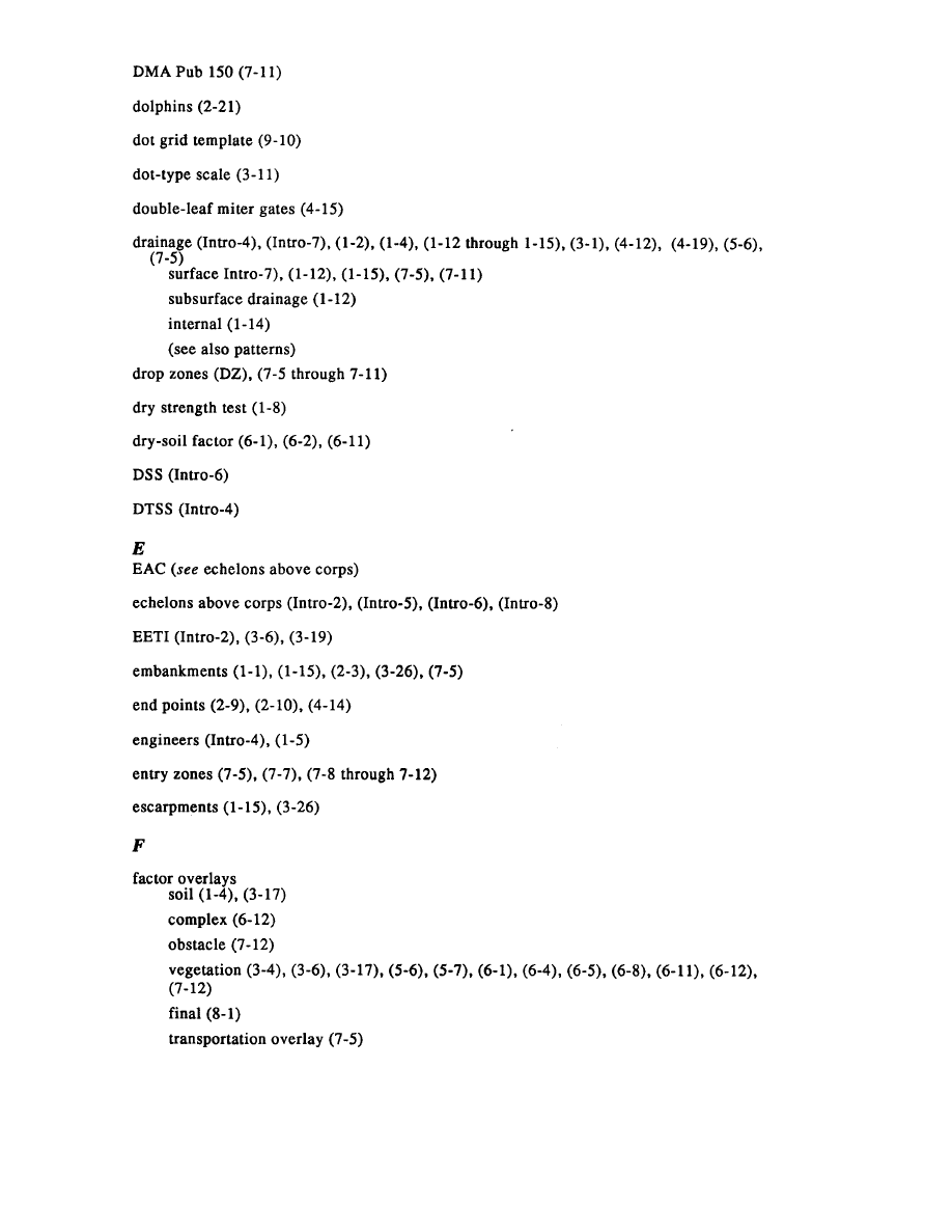
Index-4

Index-5

Index-6

Index-7

Index-8

Index-9

Index-10

Index-11

Index-12

Index-13

Index-14

FM 5-33
11 JULY 1990
By Order of the Secretary of the Army:
CARL E. VUONO
General, United States Army
Chief of Staff
Official:
WILLIAM J. MEEHAN II
Brigadier General, United States Army
The Adjutant General
DISTRIBUTION:
Active Army, USAR, and ARNG: To be distributed in accordance with DA Form 12-11-E,
requirements for FM 5-33, Terrain Analysis (Qty rqr block no. 4329); FM 30-10, Military
Geographic Intelligence (Terrain) (Qty rqr block no. 0181); and FM 21-33, Terrain Analysis (Qty
rqr block no. 0465).
U.S. Government Printing Office: 1992—311-831/61407 PIN: 047926-001
Document Outline
- Cover, FM 5-33 Terrain Analysis
- Preface
- Change 1.
- Chapter 1. Natural Terrain
- Chapter 2. Man-Made Features
- Chapter 3. Natural Terrain
- Chapter 4. Man-made Features
- Chapter 5. Lines of Communication, Cover and Concealment
- Chapter 6. Cross-Country Movement
- Chapter 7. Line of Site and Zone of Entry
- Chapter 8. Final Overlay Preparation
- Chapter 9. Vertical Photography
- Chapter 10. Mathematical Techniques
- Appendix A
- Appendix B
- Appendix C
- Glossary
- References
- Index
- Authorization
Wyszukiwarka
Podobne podstrony:
Reklama cyfrowa Podrecznik Analiza dzialan reklamowych najwiekszych swiatowych firm medialnych e 1g4
Sitemaster Kompaktowy podreczny analizator kabli i anten z analizatorem widma broszura PL
Analiza programu nauczania i podręczników- WSiP, UKW
04 SESJA analiza, Stary podrecznik klubu pracy
analiza technologiczna, Podręczniki
finanse symfonia analizy finansowe podręcznik TI5TWDWE3RQCUJPL4PKGGPTXTP3GKAKFRIJXRKQ
Analiza podręcznika Wybór podręcznika do klas IV VI
Analiza podręcznika. Wybór podręcznika do klas IV-VI
Autodesk Robot Structural Analysis 2010 Projekt moj zelbet analiza słupa Wyniki MES aktualne
FS ANALIZA FINANSOWA, FEASIBILITY STUDY- podręcznik UNIDO
Analiza i ocena wybranych podręczników
Podrecznik EXPERT Analiza ciepl Nieznany
Analiza skupień - podręcznik internetowy, Technika Rolnicza, Metody taksonometrii
Analiza programu nauczania i podręczników- JUKA, UKW
Numeryczny model terenu i operacje na strukturze GRID jako podstawa analiz hydrologicznych
Analiza podręczników
Analiza FOR 5 2014 Rzadowy podrecznik to nie oszczednoscia uzaleznienie edukacji od politykow
więcej podobnych podstron