Laboratory

8

TCP: Transmission Control Protocol

A Reliable, Connection-Oriented, Byte-Stream Service

Objective

This lab is designed to demonstrate the congestion control algorithms implemented by the
Transmission Control Protocol (TCP). The lab provides a number of scenarios to simulate
these algorithms. You will compare the performance of the algorithms through the analysis
of the simulation results.

Overview

The Internet’s TCP guarantees the reliable, in-order delivery of a stream of bytes. It
includes a flow-control mechanism for the byte streams that allows the receiver to limit
how much data the sender can transmit at a given time. In addition, TCP implements a
highly tuned congestion-control mechanism. The idea of this mechanism is to throttle how
fast TCP sends data to keep the sender from overloading the network.

The idea of TCP congestion control is for each source to determine how much capacity is
available in the network, so that it knows how many packets it can safely have in transit. It
maintains a state variable for each connection, called the congestion window, which is
used by the source to limit how much data it is allowed to have in transit at a given time.
TCP uses a mechanism, called additive increase/multiplicative decrease, that decreases
the congestion window when the level of congestion goes up and increases the
congestion window when the level of congestion goes down. TCP interprets timeouts as a
sign of congestion. Each time a timeout occurs, the source sets the congestion window to
half of its previous value. This halving corresponds to the multiplicative decrease part of
the mechanism. The congestion window is not allowed to fall below the size of a single
packet (the TCP maximum segment size, or MSS). Every time the source successfully
sends a congestion window’s worth of packets, it adds the equivalent of one packet to the
congestion window; this is the additive increase part of the mechanism.

TCP uses a mechanism called slow start to increase the congestion window “rapidly” from
a cold start in TCP connections. It increases the congestion window exponentially, rather
than linearly. Finally, TCP utilizes a mechanism called fast retransmit and fast recovery.
Fast retransmit is a heuristic that sometimes triggers the retransmission of a dropped
packet sooner than the regular timeout mechanism

In this lab you will set up a network that utilizes TCP as its end-to-end transmission
protocol and analyze the size of the congestion window with different mechanisms.

2

Procedure

Create a New Project

1. Start

OPNET IT Guru Academic Edition

⇒ Choose New from the File menu.

2. Select

Project and click OK

⇒ Name the project <your initials>_TCP, and the

scenario No_Drop

⇒ Click OK.

3. In

the

Startup Wizard: Initial Topology dialog box, make sure that Create Empty

Scenario is selected

⇒ Click Next ⇒ Select Choose From Maps from the

Network Scale list

⇒ Click Next ⇒ Choose USA from the Map List ⇒ Click Next

twice

⇒ Click OK.

Create and Configure the Network

Initialize the Network:

1. The

Object Palette dialog box should now be on the top of your project space. If it

is not there, open it by clicking

. Make sure that the internet_toolbox item is

selected from the pull-down menu on the object palette.

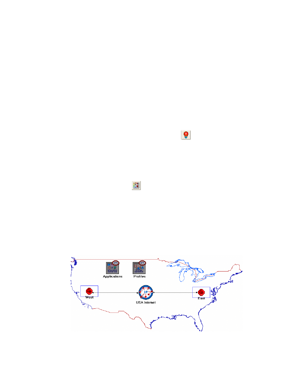
2. Add to the project workspace the following objects from the palette: Application

Config, Profile Config, an ip32_Cloud, and two subnets.

a. To add an object from a palette, click its icon in the object palette

⇒ Move your

mouse to the workspace

⇒ Click to drop the object in the desired location ⇒

Right-click to finish creating objects of that type.

3. Close the palette.

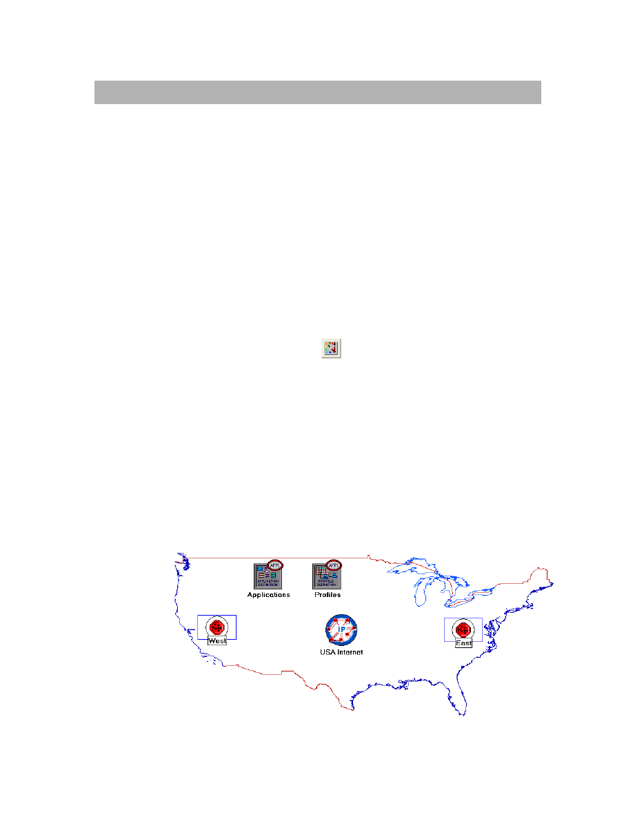
4. Rename the objects you added as shown and then save your project:

The ip32_cloud node
model represents an IP
cloud supporting up to
32 serial line interfaces at
a selectable data rate
through which IP traffic
can be modeled. IP
packets arriving on any
cloud interface are
routed to the appropriate
output interface based
on their destination IP
address. The RIP or
OSPF protocol may be
used to automatically
and dynamically create
the cloud's routing tables
and select routes in an
adaptive manner. This
cloud requires a fixed
amount of time to route
each packet, as
determined by the
Packet Latency

attribute of the node.

3

Configure the Applications:

1. Right-click on the Applications node

⇒ Edit Attributes ⇒ Expand the

Application Definitions attribute and set rows to 1

⇒ Expand the new row ⇒

Name the row FTP_Application.

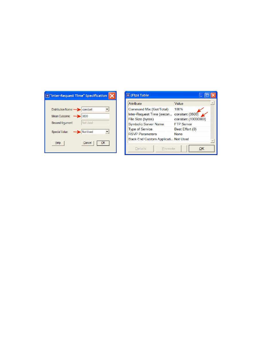
i. Expand the Description hierarchy

⇒ Edit the FTP row as shown (you will

need to set the Special Value to Not Used while editing the shown
attributes):

2. Click

OK twice and then save your project.

4

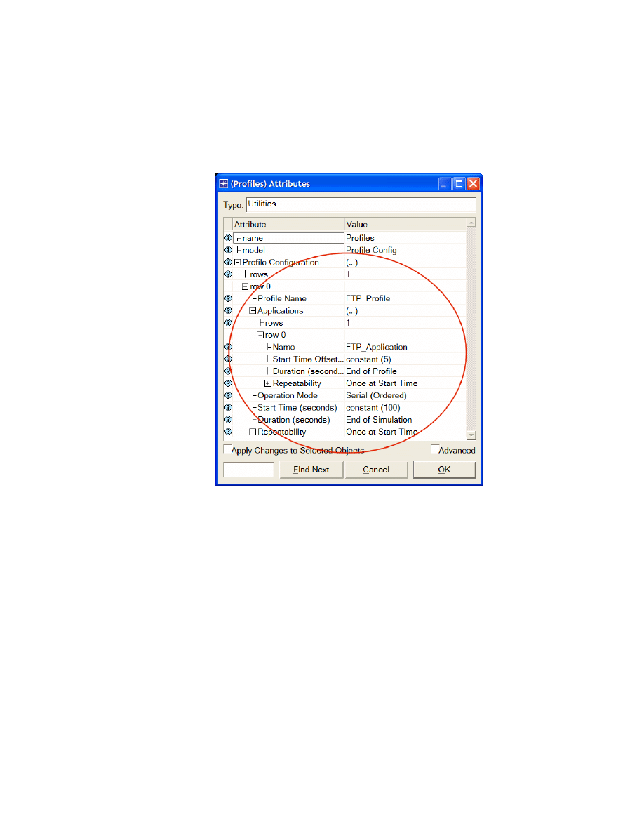
Configure the Profiles:

1. Right-click on the Profiles node

⇒ Edit Attributes ⇒ Expand the Profile

Configuration attribute and set rows to 1.

i. Name and set the attributes of row 0 as shown

⇒ Click OK.

5

Configure the West Subnet:

1. Double-click

on

the

West subnet node. You get an empty workspace, indicating

that the subnet contains no objects.

2. Open the object palette

and make sure that the internet_toolbox item is

selected from the pull-down menu.

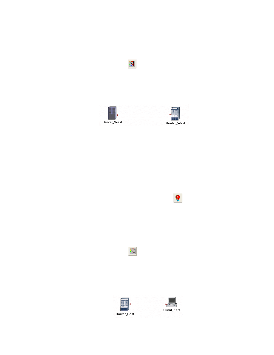
3. Add the following items to the subnet workspace: one ethernet_server, one

ethernet4_slip8_gtwy router, and connect them with a bidirectional 100_BaseT
link

⇒ Close the palette ⇒ Rename the objects as shown.

4. Right-click on the Server_West node

⇒ Edit Attributes:

i. Edit Application: Supported Services

⇒ Set rows to 1 ⇒ Set Name to

FTP_Application

⇒ Click OK.

ii. Edit the value of the Server Address attribute and write down Server_West.

iii. Expand the TCP Parameters hierarchy

⇒ Set both Fast Retransmit and

Fast Recovery to Disabled.

5. Click

OK and then save your project.

Now, you have completed the configuration of the West subnet. To go back to the top

level of the project, click the Go to next higher level

button.

Configure the East Subnet:

1. Double-click

on

the

East subnet node. You get an empty workspace, indicating

that the subnet contains no objects.

2. Open the object palette

and make sure that the internet_toolbox item is

selected from the pull-down menu.

3. Add the following items to the subnet workspace: one ethernet_wkstn, one

ethernet4_slip8_gtwy router, and connect them with a bidirectional 100_BaseT
link

⇒ Close the palette ⇒ Rename the objects as shown.

The ethernet4_slip8_
gtwy node model
represents an IP-based
gateway supporting four
Ethernet hub interfaces
and eight serial line

interfaces.

6

4. Right-click on the Client_East node

⇒ Edit Attributes:

i. Expand

the

Application: Supported Profiles hierarchy

⇒ Set rows to 1 ⇒

Expand the row 0 hierarchy

⇒ Set Profile Name to FTP_Profile.

ii. Assign

Client_ East to the Client Address attributes.

iii. Edit

the

Application: Destination Preferences attribute as follows:

Set rows to 1

⇒ Set Symbolic Name to FTP Server ⇒ Edit Actual Name ⇒

Set rows to 1

⇒ In the new row, assign Server_West to the Name column.

5. Click

OK three times and then save your project.

6. You have now completed the configuration of the East subnet. To go back to the

project space, click the Go to next higher level

button.

Connect the Subnets to the IP Cloud:

1. Open the object palette

.

2. Using

two

PPP_DS3 bidirectional links connect the East subnet to the IP Cloud

and the West subnet to the IP Cloud.

3. A pop-up dialog box will appear asking you what to connect the subnet to the IP

Cloud with. Make sure to select the “routers.”

4. Close

the

palette.

7

Choose the Statistics

1. Right-click

on

Server_West in the West subnet and select Choose Individual

Statistics from the pop-up menu.

2. In

the

Choose Results dialog box, choose the following statistic:

TCP Connection

⇒ Congestion Window Size (bytes) and Sent Segment

Sequence Number.

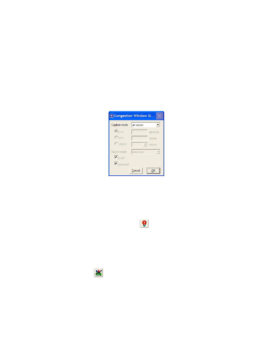
3. Right-click on the Congestion Window Size (bytes) statistic

⇒ Choose Change

Collection Mode

⇒ In the dialog box check Advanced ⇒ From the drop-down

menu, assign all values to Capture mode as shown

⇒ Click OK.

4. Right-click on the Sent Segment Sequence Number statistic

⇒ Choose

Change Collection Mode

⇒ In the dialog box check Advanced ⇒ From the

drop-down menu, assign all values to Capture mode.

5. Click

OK twice and then save your project.

6. Click

the

Go to next higher level

button.

Configure the Simulation

Here we need to configure the duration of the simulation:

1. Click

on

and the Configure Simulation window should appear.

2. Set the duration to be 10.0 minutes.

3. Click

OK and then save your project.

OPNET provides the
following capture
modes:

All values—collects
every data point from a
statistic.

Sample—collects the
data according to a user-
specified time interval or
sample count. For
example, if the time
interval is 10, data is
sampled and recorded
every 10th second. If the
sample count is 10, every
10th data point is
recorded. All other data
points are discarded.

Bucket—collects all of
the points over the time
interval or sample count
into a “data bucket” and
generates a result from
each bucket. This is the

default mode.

8

Duplicate the Scenario

In the network we just created we assumed a perfect network with no discarded packets.
Also, we disabled the fast retransmit and fast recovery techniques in TCP. To analyze the
effects of discarded packets and those congestion-control techniques, we will create two
additional scenarios.

1. Select Duplicate Scenario from the Scenarios menu and give it the name

Drop_NoFast

⇒ Click OK.

2. In the new scenario, right-click on the IP Cloud

⇒ Edit Attributes ⇒ Assign

0.05% to the Packet Discard Ratio attribute.

3. Click

OK and then save your project.

4. While you are still in the Drop_NoFast scenario, select Duplicate Scenario from

the Scenarios menu and give it the name Drop_Fast.

5. In

the

Drop_Fast scenario, right-click on Server_ West, which is inside the West

subnet

⇒ Edit Attributes ⇒ Expand the TCP Parameters hierarchy ⇒ Enable

the Fast Retransmit attribute

⇒ Assign Reno to the Fast Recovery attribute.

6. Click

OK and then save your project.

Run the Simulation

To run the simulation for the three scenarios simultaneously:

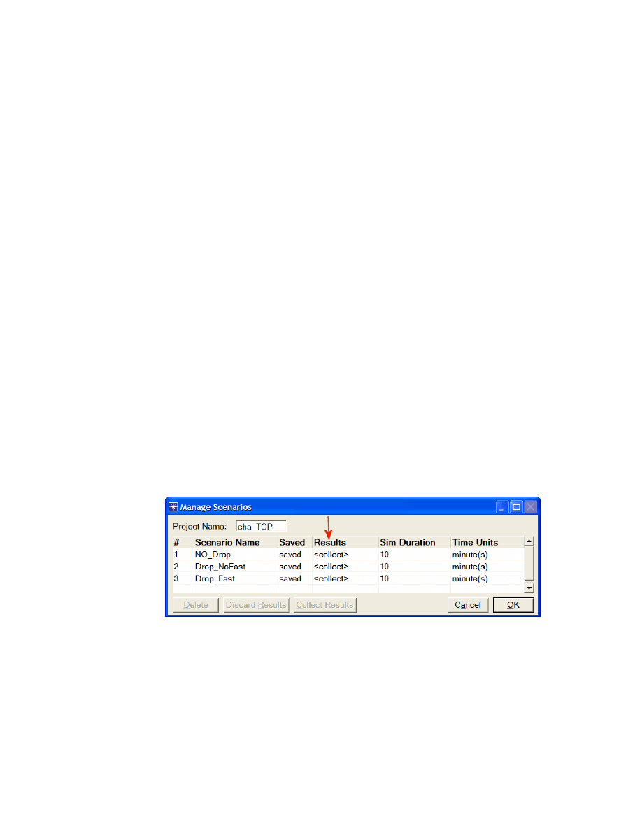
1. Go to the Scenarios menu

⇒ Select Manage Scenarios.

2. Change the values under the Results column to <collect> (or <recollect>)

for the three scenarios. Compare to the following figure.

3. Click OK to run the three simulations. Depending on the speed of your

processor, this may take several minutes to complete.

4. After the three simulation runs complete, one for each scenario, click Close

⇒

Save your project.

With fast retransmit,
TCP performs a
retransmission of what
appears to be the
missing segment,
without waiting for a
retransmission timer to
expire.

After fast retransmit
sends what appears to be
the missing segment,
congestion avoidance
but not slow start is
performed. This is the
fast recovery algorithm.

The fast retransmit and
fast recovery algorithms
are usually implemented

together (RFC 2001).

9

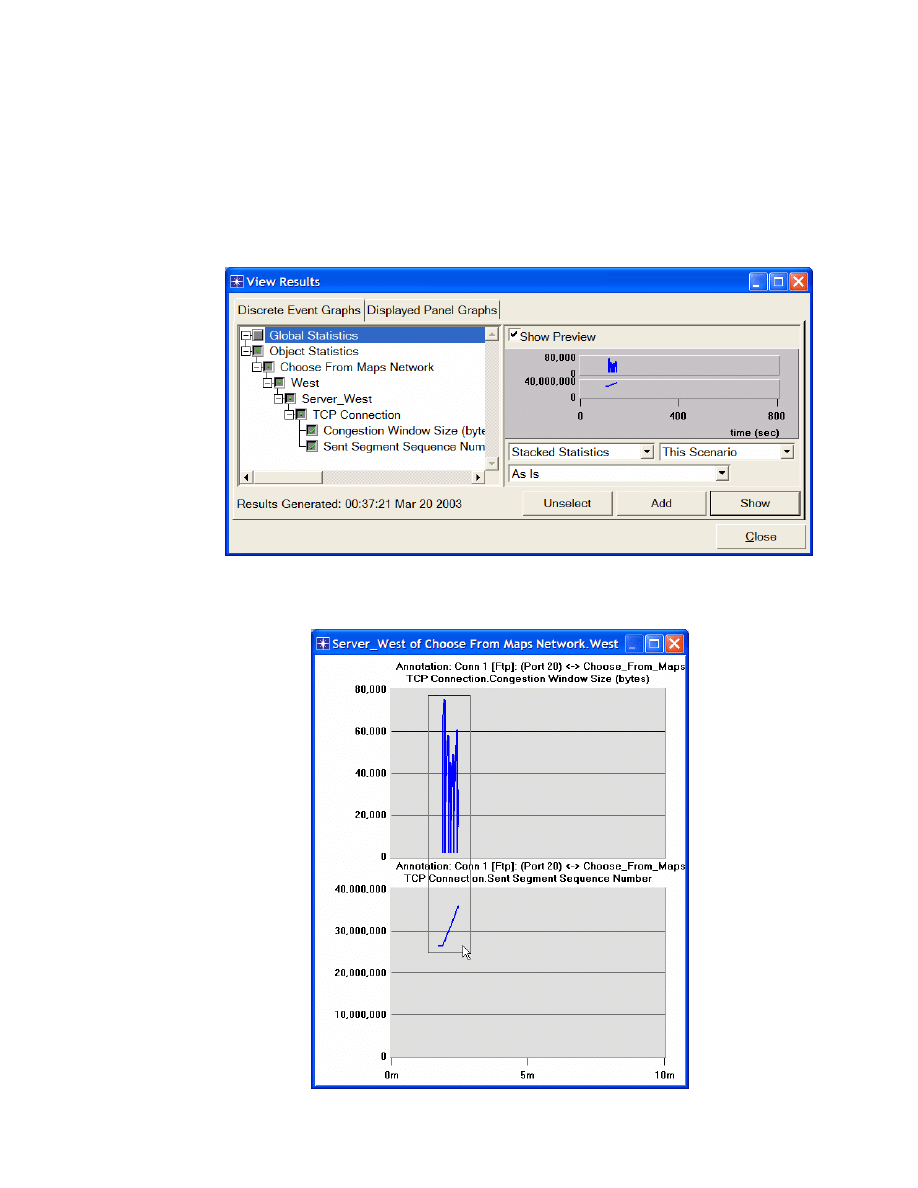
View the Results

To view and analyze the results:

1. Switch to the Drop_NoFast scenario (the second one) and choose View Results

from the Results menu.

2. Fully expand the Object Statistics hierarchy and select the following two results:

Congestion Window Size (bytes) and Sent Segment Sequence Number.

3. Click

Show. The resulting graphs should resemble the ones below.

To switch to a scenario,
choose Switch to
Scenario from the
Scenarios menu or just
press Ctrl+<scenario
number>.

10

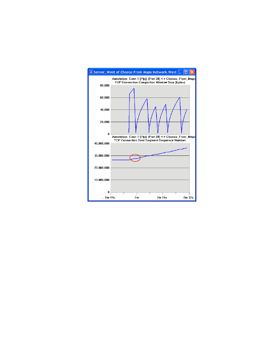
4. To zoom in on the details in the graph, click and drag your mouse to draw a

rectangle, as shown above.

5. The graph should be redrawn to resemble the following one:

6. Notice

the

Segment Sequence Number is almost flat with every drop in the

congestion window.

11

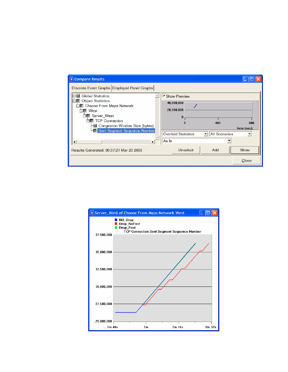
7. Close

the

View Results dialog box and select Compare Results from the Result

menu.

8. Fully expand the Object Statistics hierarchy as shown and select the following

result: Sent Segment Sequence Number.

9. Click

Show. After zooming in, the resulting graph should resemble the one below.

12

Further Readings

- OPNET TCP Model Description: From the Protocols menu, select TCP

⇒

Model Usage Guide.

-

Transmission Control Protocol: IETF RFC number 793 (www.ietf.org/rfc.html).

Questions

1)

Why does the Segment Sequence Number remain unchanged (indicated by a
horizontal line in the graphs) with every drop in the congestion window?

2)

Analyze the graph that compares the Segment Sequence numbers of the three
scenarios. Why does the Drop_NoFast scenario have the slowest growth in
sequence numbers?

3)

In the Drop_NoFast scenario, obtain the overlaid graph that compares Sent
Segment Sequence Number with Received Segment ACK Number for
Server_West. Explain the graph.

Hint:

- Make sure to assign all values to the Capture mode of the Received

Segment ACK Number statistic.

4)

Create another scenario as a duplicate of the Drop_Fast scenario. Name the
new scenario Q4_Drop_Fast_Buffer. In the new scenario, edit the attributes of
the Client_East node and assign 65535 to its Receiver Buffer (bytes) attribute
(one of the TCP Parameters). Generate a graph that shows how the
Congestion Window Size (bytes) of Server_West gets affected by the increase
in the receiver buffer (compare the congestion window size graph from the
Drop_Fast

scenario

with the corresponding graph from the

Q4_Drop_Fast_Buffer scenario.)

Lab Report

Prepare a report that follows the guidelines explained in Lab 0. The report should include
the answers to the above questions as well as the graphs you generated from the
simulation scenarios. Discuss the results you obtained and compare these results with
your expectations. Mention any anomalies or unexplained behaviors.