
Technical Report No. 84 / Rapport technique n
o
84
Yield Curve Modelling at the Bank of Canada
by David Bolder and David Stréliski
Bank of Canada
Banque du Canada


The views expressed in this report are solely those of the authors.
No responsibility for them should be attributed to the Bank of Canada.
February 1999
Yield Curve Modelling at the Bank of Canada
David Bolder and David Stréliski

Printed in Canada on recycled paper
ISSN 0713-7931
ISBN 0-662-27602-7

CONTENTS
iii
ACKNOWLEDGEMENTS.........................................................................v
ABSTRACT / RÉSUMÉ .......................................................................... vii
1. INTRODUCTION .......................................................................................1
2. THE MODELS ............................................................................................2
2.1
The Super-Bell model .........................................................................2
2.2
The Nelson-Siegel and Svensson models ...........................................4
3. DATA
..................................................................................................14
3.1
Description of the Canadian data......................................................15
3.2
Why are the data important? .............................................................16
3.3
Approaches to the filtering of data....................................................17
3.3.1 Severity of data filtering: Divergence from par and
amount outstanding..................................................................17
3.3.2 The short-end: Treasury bills and short-term bonds ................18
4. EMPIRICAL RESULTS ............................................................................19
4.1
The “estimation problem”.................................................................20
4.1.1
Robustness of solution ..........................................................23
4.1.2
Goodness of fit ......................................................................25
4.1.3
Speed of estimation...............................................................29
4.1.4
The “estimation” decision.....................................................31
4.2
The “data problem”...........................................................................31
4.2.1
Tightness of data filtering .....................................................33
4.2.2
Data filtering at the short-end of the term structure..............35
4.2.3
The “data” decision...............................................................37
5. CONCLUDING REMARKS.....................................................................37
TECHNICAL APPENDIXES ...................................................................39
A.
Basic “yield curve” building blocks..................................................39
A.1
Zero-coupon rate and discount factors..................................39
A.2
Yield to maturity and the “coupon effect” ............................40
A.3
Duration ................................................................................42
A.4
Par yields...............................................................................42
B.
Extracting zero-coupon rates from the par yield curve.....................43
C.
Extracting “implied” forward rates from zero-coupon rates.............45

iv
D.
Mechanics of the estimation .............................................................46
D.1
Construction of theoretical bond prices ................................46
D.2
Log-likelihood objective function.........................................47
D.3
Sum of squared errors with penalty parameter
objective function..................................................................48
E.
Optimization algorithms ...................................................................49
E.1
Full-estimation algorithm .....................................................50
E.2
Partial-estimation algorithm..................................................51
REFERENCES ..........................................................................................55

v
ACKNOWLEDGEMENTS
We would like to thank John Kiff, Richard Black, Des McManus,
Mark Zelmer, and Jean-François Fillion from the Bank of Canada as well as
Burton Hollifield from Carnegie Mellon University for his suggestions on
an early draft of this work that was presented at the University of British
Columbia in the spring of 1998. We also appreciated the input from co-op
student James Mott from the École des Hautes Études Commerciales de
Montréal.


vii
ABSTRACT
The primary objective of this paper is to produce a framework that could be
used to construct a historical data base of zero-coupon and forward yield curves
estimated from Government of Canada securities’ prices. The secondary objective
is to better understand the behaviour of a class of parametric yield curve models,
specifically, the Nelson-Siegel and the Svensson methodologies. These models
specify a functional form for the instantaneous forward interest rate, and the user
must determine the function parameters that are consistent with market prices for
government debt. The results of these models are compared with those of a yield
curve model used by the Bank of Canada for the last 15 years. The Bank of Can-
ada’s existing model, based on an approach developed by Bell Canada, fits a so-
called “par yield” curve to bond yields to maturity and subsequently extracts zero-
coupon and “implied forward” rates. Given the pragmatic objectives of this
research, the analysis focuses on the practical and deals with two key problems: the
estimation problem (the choice of the best yield curve model and the optimization
of its parameters); and the data problem (the selection of the appropriate set of mar-
ket data). In the absence of a developed literature dealing with the practical side of
parametric term structure estimation, this paper provides some guidance for those
wishing to use parametric models under “real world” constraints.
In the analysis of the estimation problem, the data filtering criteria are held
constant (this is the “benchmark” case). Three separate models, two alternative
specifications of the objective function, and two global search algorithms are exam-
ined. Each of these nine alternatives is summarized in terms of goodness of fit,
speed of estimation, and robustness of the results. The best alternative is the Sven-
sson model using a price-error-based, log-likelihood objective function and a global
search algorithm that estimates subsets of parameters in stages. This estimation
approach is used to consider the data problem. The authors look at a number of
alternative data filtering settings, which include a more severe or “tight” setting and
an examination of the use of bonds and/or treasury bills to model the short-end of
the term structure. Once again, the goodness of fit, robustness, and speed of estima-
tion are used to compare these different filtering possibilities. In the final analysis,
it is decided that the benchmark filtering setting offers the most balanced approach
to the selection of data for the estimation of the term structure.
This work improves the understanding of this class of parametric models
and will be used for the development of a historical data base of estimated term
structures. In particular, a number of concerns about these models have been
resolved by this analysis. For example, the authors believe that the log-likelihood

viii
specification of the objective function is an efficient approach to solving the esti-
mation problem. In addition, the benchmark data filtering case performs well rela-
tive to other possible filtering scenarios. Indeed, this parametric class of models
appears to be less sensitive to the data filtering than initially believed. However,
some questions remain; specifically, the estimation algorithms could be improved.
The authors are concerned that they do not consider enough of the domain of the
objective function to determine the optimal set of starting parameters. Finally,
although it was decided to employ the Svensson model, there are other functional
forms that could be more stable or better describe the underlying data. These two
remaining questions suggest that there are certainly more research issues to be
explored in this area.

ix
RÉSUMÉ
Le principal objectif des auteurs est d’établir un cadre d’analyse permettant
d’élaborer une base de données chronologiques relative aux courbes théoriques de
taux de rendement coupon zéro et de taux à terme estimées à partir des cours des
titres du gouvernement canadien. Les auteurs cherchent également à mieux com-
prendre le comportement de la catégorie des modèles paramétriques de courbe de
rendement, plus précisément, le modèle de Nelson et Siegel et celui de Svensson.
Ces modèles définissent une forme fonctionnelle pour la courbe des taux d’intérêt
à terme instantanés, et l’utilisateur doit déterminer les valeurs des paramètres de la
fonction qui sont compatibles avec les prix des titres du gouvernement sur le mar-
ché. Les résultats obtenus à l’aide de ces modèles sont comparés à ceux du modèle
de courbe de rendement que la Banque du Canada utilise depuis quinze ans. Le
modèle actuel de la Banque, qui s’inspire d’une approche élaborée par Bell
Canada, estime une courbe de « rendement au pair » à partir des taux de rendement
à l’échéance des obligations puis en déduit les taux de rendement coupon zéro et
les « taux à terme implicites ». Étant donné l’aspect pragmatique des objectifs
visés, l’analyse est centrée sur deux importants problèmes d’ordre pratique : le
problème de l’estimation (le choix du meilleur modèle pour représenter la courbe
de rendement et de la méthode d’optimisation des paramètres) et le problème du
choix des données (c’est-à-dire la sélection d’un échantillon approprié parmi les
données du marché). Vu l’absence d’une littérature abondante traitant des aspects
pratiques de l’estimation de modèles paramétriques relatifs à la structure des taux
d’intérêt, les auteurs fournissent quelques conseils à l’intention de ceux qui
désirent utiliser les modèles paramétriques dans le cadre des contraintes du
« monde réel ».
Pour analyser le problème de l’estimation, les auteurs fixent les critères de
filtrage des données (il s’agit de leur « formule de référence » pour le filtrage) et
examinent trois modèles distincts, deux spécifications différentes de la fonction
objectif et deux algorithmes de recherche globale. Les résultats obtenus à partir de
chacun des neuf schémas envisagés sont évalués en fonction de leur robustesse, de
l’adéquation statistique et de la vitesse d’estimation. Le schéma qui donne les
meilleurs résultats est le modèle de Svensson qui comporte 1) une fonction objectif
de type fonction de vraisemblance logarithmique basée sur les erreurs de prix et
2) un algorithme de recherche globale qui estime les sous-ensembles de paramè-
tres par étapes. Les auteurs font ensuite appel à ce schéma d’estimation pour analy-
ser le problème du choix des données. Ils se penchent sur un certain nombre de
combinaisons différentes des critères de filtrage des données; ils utilisent un
ensemble de critères de filtrage très contraignants d’une part et cherchent à établir

x
d’autre part si la portion à court terme de la structure des taux est mieux modélisée
à l’aide des obligations ou des bons du Trésor (ou des deux types de titres). Les
différentes formules de filtrage sont elles aussi comparées entre elles sous l’angle
de l’adéquation statistique, de la robustesse et de la vitesse d’estimation. Les
auteurs concluent en définitive que la formule de filtrage de référence est la mieux
adaptée au choix des données qui serviront à l’estimation de la structure des taux.
Le travail des auteurs contribue à améliorer la compréhension de ce type de
modèles paramétriques et permettra d’élaborer une base de données chrono-
logiques relative aux structures de taux estimées. Un certain nombre de questions
soulevées par ces modèles ont été résolues dans l’étude. Par exemple, les auteurs
croient que la spécification d’une fonction objectif de type fonction de vraisem-
blance logarithmique est une approche efficace pour résoudre le problème de
l’estimation. De plus, la formule de filtrage de référence donne de bons résultats
comparativement aux autres formules. Cette catégorie de modèles paramétriques
semble en effet moins sensible que prévu au filtrage des données. Toutefois,
certaines questions demeurent. En particulier, les algorithmes d’estimation peu-
vent encore être améliorés. Les auteurs craignent de ne pas avoir couvert une assez
grande portion de l’espace de la fonction objectif pour trouver l’ensemble optimal
des valeurs de départ des paramètres. En outre, bien qu’ils aient décidé d’utiliser le
modèle de Svensson, il se peut que d’autres formes fonctionnelles se révèlent plus
stables ou mieux en mesure d’expliquer les données sous-jacentes. Ces deux
derniers points laissent croire qu’il subsiste d’autres questions qui méritent d’être
explorées dans ce domaine.

1
1.
INTRODUCTION
Zero-coupon and forward interest rates are among the most fundamental tools in finance.
Applications of zero-coupon and forward curves include measuring and understanding market
expectations to aid in the implementation of monetary policy; testing theories of the term
structure of interest rates; pricing of securities; and the identification of differences in the theo-
retical value of securities relative to their market value. Unfortunately, zero-coupon and forward
rates are not directly observable in the market for a wide range of maturities. They must,
therefore, be estimated from existing bond prices or yields.
A number of estimation methodologies exist to derive the zero-coupon and forward curves
from observed data. Each technique, however, can provide surprisingly different shapes for these
curves. As a result, the selection of a specific estimation technique depends on its final use. The
main interest of this paper in the term structure of interest rates relates to how it may be used to
provide insights into market expectations regarding future interest rates and inflation. Given that
this application does not require pricing transactions, some accuracy in the “goodness of fit” can
be foregone for a more parsimonious and easily interpretable form. It is nevertheless important
that the estimated forward and zero-coupon curves fit the data well.
The primary objective of this paper is to produce a framework that could be used to gen-
erate a historical data base of zero-coupon and forward curves estimated from Government of
Canada securities’ prices. The purpose of this research is also to better understand the behaviour
of a different class of yield curve model in the context of Canadian data. To meet these objectives,
this paper revisits the Bank of Canada’s current methodology for estimating Canadian gov-
ernment zero-coupon and forward curves. It introduces and compares this methodology with
alternative approaches to term structure modelling that rely upon a class of parametric models,
specifically, the Nelson-Siegel and the Svensson methodologies.
The Bank’s current approach utilizes the so-called Super-Bell model for extracting the
zero-coupon and forward interest rates from Government of Canada bond yields. This approach
uses essentially an ordinary least-squares (OLS) regression to fit a par yield curve from existing
bond “yields to maturity” (YTM). It then employs a technique termed “bootstrapping” to derive
zero-coupon rates and subsequently implied forward rates. The proposed models are quite dif-
ferent from the current approach and begin with a specified parametrized functional form for the
instantaneous forward rate curve. From this functional form, described later in the text, a con-
tinuous zero-coupon rate function and its respective discount function are derived. An optimi-
zation process is used to determine the appropriate parameters for these functions that best fit the
existing bond prices.

2
The research has pragmatic objectives, so the focus throughout the analysis is highly prac-
tical. It deals with two key problems: the estimation problem, or the choice of the best yield curve
model and the optimization of its parameters; and the data problem, or the selection of the appro-
priate set of market data. The wide range of possible filtering combinations and estimation
approaches makes this a rather overwhelming task. Therefore, examination is limited to a few
principal dimensions. Specifically, the analysis begins with the definition of a “benchmark” fil-
tering case. Using this benchmark, the estimation problem is examined by analyzing different
objective function specifications and optimization algorithms. After this analysis, the best optimi-
zation approach is selected and used to consider two different aspects of data filtering. To accom-
plish this, different data filtering scenarios are contrasted with the initial benchmark case.
Section 2 of the paper introduces the current Super-Bell model and the proposed Nelson-
Siegel and Svensson models and includes a comparison of the two modelling approaches.
Section 3 follows with a description of Canada bond and treasury bill data. This section also
details the two primary data filtering dimensions: the severity of data filtering, and the selection of
observations at the short-end of the maturity spectrum. The empirical results, presented in
Section 4, begin with the treatment of the estimation problem followed by the data problem. The
final section, Section 5, presents some concluding remarks.
2.
THE MODELS
The following section details how the specific yield curve models selected are used to
extract theoretical zero-coupon and forward interest rates from observed bond and treasury bill
prices. The new yield curve modelling methodology introduced in this section is fundamentally
different from the current Super-Bell model. To highlight these differences, the current method-
ology is discussed briefly and then followed by a detailed description of the new approach. The
advantages and disadvantages of each approach are also briefly detailed.
2.1
The Super-Bell model
The Super-Bell model, developed by Bell Canada Limited in the 1960s, is quite straight-
forward. It uses an OLS regression of yields to maturity on a series of variables including power
transformations of the term to maturity and two coupon terms. The intent is to derive a so-called
par yield curve.
1
A par yield curve is a series of yields that would be observed if the sample of
bonds were all trading at par value. The regression equation is as follows:
(EQ 1)
1.
See Section A.4, “Par yields,” on page 42 in the technical appendix for a complete definition of par yields.
Y
M C
,
β
0
β
1
M
( ) β
2
M
2
(
) β
3
M
3
(
) β
4
M
0.5
(
) β
+
5
M
log
(
) β
6
C
( ) β
7
C M
⋅
(
) ε
+
+
+
+
+
+
+
=

3
This regression defines yield to maturity (Y
M,C
) as a function of term to maturity (M) and
the coupon rate (C). Once the coefficients (
β
0
through
β
6
) have been estimated, another regression
is performed to extract the par yields. By definition, a bond trading at par has a coupon that is
equal to the yield (that is, Y
M,C
= C). As a result, the expression above can be rewritten as follows:
(EQ 2)
Using the coefficients estimated from the first equation and the term to maturity for each
bond, a vector of par yields (Y
M
) is obtained through this algebraic rearrangement of the original
regression equation. The second step uses this vector of par yields and runs an additional esti-
mation, using the same term-to-maturity variables but without the coupon variables as follows to
create a “smoothed” par yield curve:
(EQ 3)
In 1987, however, an adjustment was made to the par yield estimation. Specifically, a dif-
ferent estimation is used to obtain a par yield vector for bonds with a term to maturity of 15 years
and greater. The following specification is used, making the explicit assumption that the term to
maturity is a linear function of the coupon rate.
2
The impact of this approach, which makes the
coupon effect constant for all bonds with terms to maturity of 15 years and greater, is to flatten out
the long end of the yield curve.
(EQ 4)
The par yield values for longer-term bonds are therefore solved using the same assumption
of Y
M,C
= C, as follows:
(EQ 5)
The par yield values are combined for all maturities and the new par yield curve is esti-
mated using the same approach as specified above in equation (2). From these estimated coeffi-
cients, the corresponding theoretical par yields can be obtained for any set of maturities.
2.
This is unlike the specification for yields with a term to maturity of less than 15 years where the coupon effect is
permitted to take a non-linear form.
Y
M
β
0
β
1
M
( ) β
2
M
2
(
) β
3
M
3
(
) β
4
M
0.5
(
) β
+
5
M
log
(
)
+
+
+
+
1
β
6
β
7
M
( )
+
–
--------------------------------------------------------------------------------------------------------------------------------------------------
ε
+
=
Y
M
β
0
β
1
M
( ) β
2
M
2
(
) β
3
M
3
(
) β
4
M
0.5
(
) β
+
5
M
log
(
)
ε
+
+
+
+
+
=
Y
M
15
>
C
,
β
0
β
1
C
( ) ε
+
+
=
Y
M
15
>
β
0
1
β
1
–
--------------
=

4
The determination of the par yield curve is only the first step in calculating zero-coupon
and forward interest rates. The next step is to extract the zero-coupon rates from the constant
maturity par yield curve, using a technique termed “bootstrapping.” Bootstrapping provides zero-
coupon rates for a series of discrete maturities. In the final step, the theoretical zero-coupon rate
curve is used to calculate implied forward rates for the same periodicity. Implied forward rate cal-
culation and bootstrapping are described in the Technical Appendix of this paper.
Advantages of the Super-Bell model, which dates back more than 25 years, include the
following:
•
The model is not conceptually difficult.
•
The model is parametrized analytically and is thus straightforward to solve.
There are, however, several criticisms of the Super-Bell model:
•
The resulting forward curve is a by-product of a lengthy process rather than the primary
output of the Super-Bell model.
•
The Super-Bell model focuses exclusively on YTM rather than on the actual cash flows of
the underlying bonds.
•
The zero-coupon curve can be derived only for discrete points in time. It is, therefore,
necessary to make additional assumptions to interpolate between the discrete zero-coupon
rates.
As a consequence of these shortcomings, the Super-Bell model can lead to forward curves
with very strange shapes (particularly at longer maturities) and poor fit of the underlying bond
prices or yields.
2.2
The Nelson-Siegel and Svensson models
The basic parametric model presented in this paper was developed by Charles Nelson and
Andrew Siegel of the University of Washington in 1987. The Svensson model is an extension of
this previous methodology.
3
Since the logic underlying the models is identical, the text will focus
on the more sophisticated Svensson model.
3.
As a result, the Svensson model is often termed the extended Nelson and Siegel model. This terminology is
avoided in the current paper because other possible extensions to the base Nelson and Siegel model exist. See
Nelson and Siegel (1987) and Svensson (1994).

5
Continuous interest rate concepts are critically important to any understanding of the
Nelson-Siegel and Svensson methodologies. Consequently, these concepts will be briefly intro-
duced prior to the models being described. In general practice, interest rates are compounded at
discrete intervals. In order to construct continuous interest rate functions (i.e., a zero-coupon or
forward interest rate curve), the compounding frequency must also be made continuous. It should
be noted, however, that the impact on zero-coupon and forward rates due to the change from semi-
annual to continuous compounding is not dramatic.
4
On a continuously compounded basis, the zero-coupon rate z(t,T) can be expressed as a
function of the discretely compounded zero-coupon rate Z(t,T) and the term to maturity, T, as
follows:
(EQ 6)
The continuously compounded discount factor can be similarly expressed:
(EQ 7)
The forward rate can also be represented as a continuously compounded rate:
(EQ 8)
Another important concept is the instantaneous forward rate (
)
. This is the
limit of the previous expression (shown in equation 8) as the term to maturity of the forward con-
tract tends towards zero:
(EQ 9)
The instantaneous forward rate can be defined as the marginal cost of borrowing (or mar-
ginal revenue from lending) for an infinitely short period of time. In practice, it would be equiv-
alent to a forward overnight interest rate. The continuously compounded zero-coupon rate for the
same period of time, z(t,T), is the average cost of borrowing over this period. More precisely, the
zero-coupon rate at time t with maturity T is equal to the average of the instantaneous forward
rates with trade dates between time t and T. The standard relationship between marginal and
4.
For example, a 10-year zero-coupon bond discounted with a 10 per cent, 10-year annually compounded zero-
coupon rate has a price of $38.54. The same zero-coupon bond discounted with a 10 per cent, 10-year
continuously compounded zero-coupon rate has a price of $36.79.
z t T
,
(
)
e
Z t T
,
(
)
100
-----------------
T
t
–
(
)
365
⁄
⋅
=
disc t T
,
(
)
e
Z t T
,
(
)
100
-----------------
T
t
–
(
)
365
⁄
⋅
–
=
f t
τ
T
, ,
(
)
T
t
–
(
)
z t T
,
(
)
⋅
[
]
τ
t
–
(
)
z t
τ
,
(
)
⋅
[
]
–
T
τ
–
----------------------------------------------------------------------------------------
=
f t
τ
T
, ,
(
)
INST
f t
τ
T
, ,
(
)
INST
f t
τ
T
, ,
(
)
τ
T
→
lim
=

6
average cost can be shown to hold between forward rates (marginal cost) and zero-coupon rates
(average cost); that is, the instantaneous forward rate is the first derivative of the zero-coupon rate
with respect to term to maturity. Thus, if equation 6 is differentiated with respect to time, the fol-
lowing expression will be obtained:
(EQ 10)
Equivalently, the zero-coupon rate is the integral of the instantaneous forward rate in the
interval from settlement (time t) to maturity (time T), divided by the number of periods to
determine a period zero-coupon rate. It is summarized as follows:
(EQ 11)
This important relationship between zero-coupon and instantaneous forward rates is a
critical component of the Nelson-Siegel and Svensson models.
The Svensson model is a parametric model that specifies a functional form for the instan-
taneous forward rate, f(TTM), which is a function of the term to maturity (TTM). The functional
form is as follows:
5
(EQ 12)
The original motivation for this modelling method was a desire to create a parsimonious
model of the forward interest rate curve that could capture the range of shapes generally seen in
yield curves: a monotonic form, humps at various areas of the curve, and s-shapes. This is one
possibility among numerous potential functional forms that could be used to fit a term structure.
The Svensson model is a good choice, given its ability to capture the stylized facts describing the
behaviour of the forward curve.
6
This model has six parameters that must be estimated,
β
0
,
β
1
,
β
2
,
β
3
,
τ
1
, and
τ
2
. As illus-
trated in Figure 1, these parameters identify four different curves, an asymptotic value, the general
5.
f(TTM)
t
is the functional equivalent of f(t,
τ
,T)
INST
with (
τ
-t)
→
(T-t) = TTM
.
6.
Note, however, that this approach is essentially an exercise in curve fitting, guided by stylized facts, and is not
directed by any economic theory.
f t
τ
T
, ,
(
)
INST
z t T
,
(
)
T
t
–
(
)
z t T
,
(
)
∂
t
∂
-------------------
⋅
+
=
z t T
,
(
)
f t
τ
T
, ,
(
)
INST
x
d
x
t
=
T
∫
T
t
–
--------------------------------------------------------
=
f TTM
(
)
t
β
0
β
1
e
TTM
τ
1
------------
–
β
2
TTM
τ
1
------------ e
TTM
τ
1
------------
–
β
3
TTM
τ
2
------------ e
TTM
τ
2
------------
–
+
+
+
=

7
shape of the curve, and two humps or U-shapes, which are combined to produce the Svensson
instantaneous forward curve for a given date. The impact of these parameters on the shape of the
forward curve can be described as follows:
7
•
β
0
= This parameter, which must be positive, is the asymptotic value of f(TTM)
t
. The curve
will tend towards the asymptote as the TTM approaches infinity.
•
β
1
= This parameter determines the starting (or short-term) value of the curve in terms of
deviation from the asymptote. It also defines the basic speed with which the curve tends
towards its long-term trend. The curve will have a negative slope if this parameter is
positive and vice versa. Note that the sum of
β
0
and
β
1
is the vertical intercept.
•
τ
1
= This parameter, which must also be positive, specifies the position of the first hump or
U-shape on the curve.
•
β
2
= This parameter determines the magnitude and direction of the hump. If
β
2
is positive,
a hump will occur at
τ
1
whereas, if
β
2
is negative, a U-shaped value will occur at
τ
1
.
•
τ
2
= This parameter, which must also be positive, specifies the position of the second hump
or U-shape on the curve.
•
β
3
= This parameter, in a manner analogous to
β
2
, determines the magnitude and direction
of the second hump.
7.
The difference between the Nelson-Siegel (one-hump) and Svensson (two-hump) versions of the model is the
functional form of the forward curve. In the one-hump version, the forward curve is defined as follows:
As a result, this model has only four parameters that require estimation; the
β
3
and
τ
2
parameters do not exist in
this model (i.e.,
β
2
and
τ
2
equal zero in the Nelson-Siegel model).
f
TTM
(
)
t
β
0
β
1
e
TTM
τ
1
------------
–
β
2
TTM
τ
1
------------ e
TTM
τ
1
------------
–
+
+
=
8
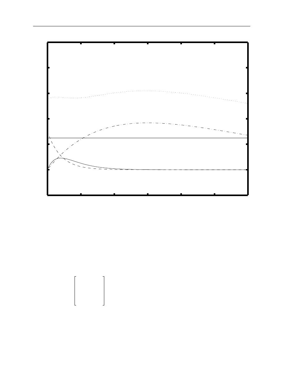
Figure 1. A decomposition of the forward term structure functional form
Having specified a functional form for the instantaneous forward rate, a zero-coupon
interest rate function is derived. This is accomplished by integrating the forward function. As pre-
viously discussed, this is possible, given that the instantaneous forward rate (which is simply the
marginal cost of borrowing) is the first derivative of the zero-coupon rate (which is similarly the
average cost of borrowing over some interval). This function is summarized as follows:
(EQ 13)
0
5
10
15
20
25
30
−2
0
2
4
6
8
10
p
Term to Maturity
Instantaneous Forward Interest Rate (%)
↑
β
0
(constant term)
↓
β
0
+
β
1
e
−TTM/
τ
1
+
β
2
(TTM/
τ
1
)e
−TTM/
τ
1
+
β
3
(TTM/
τ
2
)e
−TTM/
τ
2
(forward curve)
↓
β
1
e
−TTM/
τ
1
(first term)
↑
β
2
(TTM/
τ
1
)e
−TTM/
τ
1
(second term)
↓
β
3
(TTM/
τ
2
)e
−TTM/
τ
2
(third term)
z TTM
(
)
t
β
0
β
1
1
e
TTM
–
τ
1
---------------
–
TTM
(
) τ
1
⁄
---------------------------------
β
2
1
e
–
TTM
–
τ
1
---------------
TTM
(
) τ
1
⁄
---------------------------------
e
TTM
–
τ
1
---------------
–
β
3
1
e
–
TTM
–
τ
2
---------------
TTM
(
) τ
2
⁄
---------------------------------
e
TTM
–
τ
2
---------------
–
+
+
+
=

9
It is then relatively straightforward to determine the discount function from the zero-
coupon function.
(EQ 14)
Once the functional form is specified for the forward rate, it permits the determination of
the zero-coupon function and finally provides a discount function. The discount function permits
the discounting of any cash flow occurring throughout the term-to-maturity spectrum.
The instantaneous forward rate, zero-coupon, and discount factor functions are closely
related, with the same relationship to the six parameters. The zero-coupon and discount factor
functions are merely transformations of the original instantaneous forward rate function. The dis-
count function is the vehicle used to determine the price of a set of bonds because the present
value of a cash flow is calculated by taking the product of this cash flow and its corresponding dis-
count factor. The application of the discount factor function to all the coupon and principal pay-
ments that comprise a bond provides an estimate of the price of the bond. The discount factor
function, therefore, is the critical element of the model that links the instantaneous forward rate
and bond prices.
Every different set of parameter values in the discount rate function (which are equiva-
lently different in the zero-coupon and instantaneous forward rate functions) translates into dif-
ferent discount factors and thus different theoretical bond prices. What is required is to determine
those parameter values that are most consistent with observed bond prices. The basic process of
determining the optimal parameters for the original forward function that best fit the bond data is
outlined as follows:
8
A.
A vector of starting parameters [
β
0
,
β
1
,
β
2
,
β
3
,
τ
1
,
τ
2
] is selected.
B.
The instantaneous forward rate, zero-coupon, and discount factor functions are determined,
using these starting parameters.
C.
The discount factor function is used to determine the present value of the bond cash flows
and thereby to determine a vector of theoretical bond prices.
D.
Price errors are calculated by taking the difference between the theoretical and observed
prices.
8.
For more details of this process, see Technical Appendix, Section D, “Mechanics of the estimation,” on page 46.
disc TTM
(
)
t
e
z TTM
(
)
t
100
----------------------
TTM
(
)
⋅
–
=
10
E.
Two different numerical optimization procedures, discussed later in greater detail, are used
to minimize the decision variable subject to certain constraints on the parameter values.
9
F.
Steps B through E are repeated until the objective function is minimized.
The final parameter estimates are used to determine and plot the desired zero-coupon and
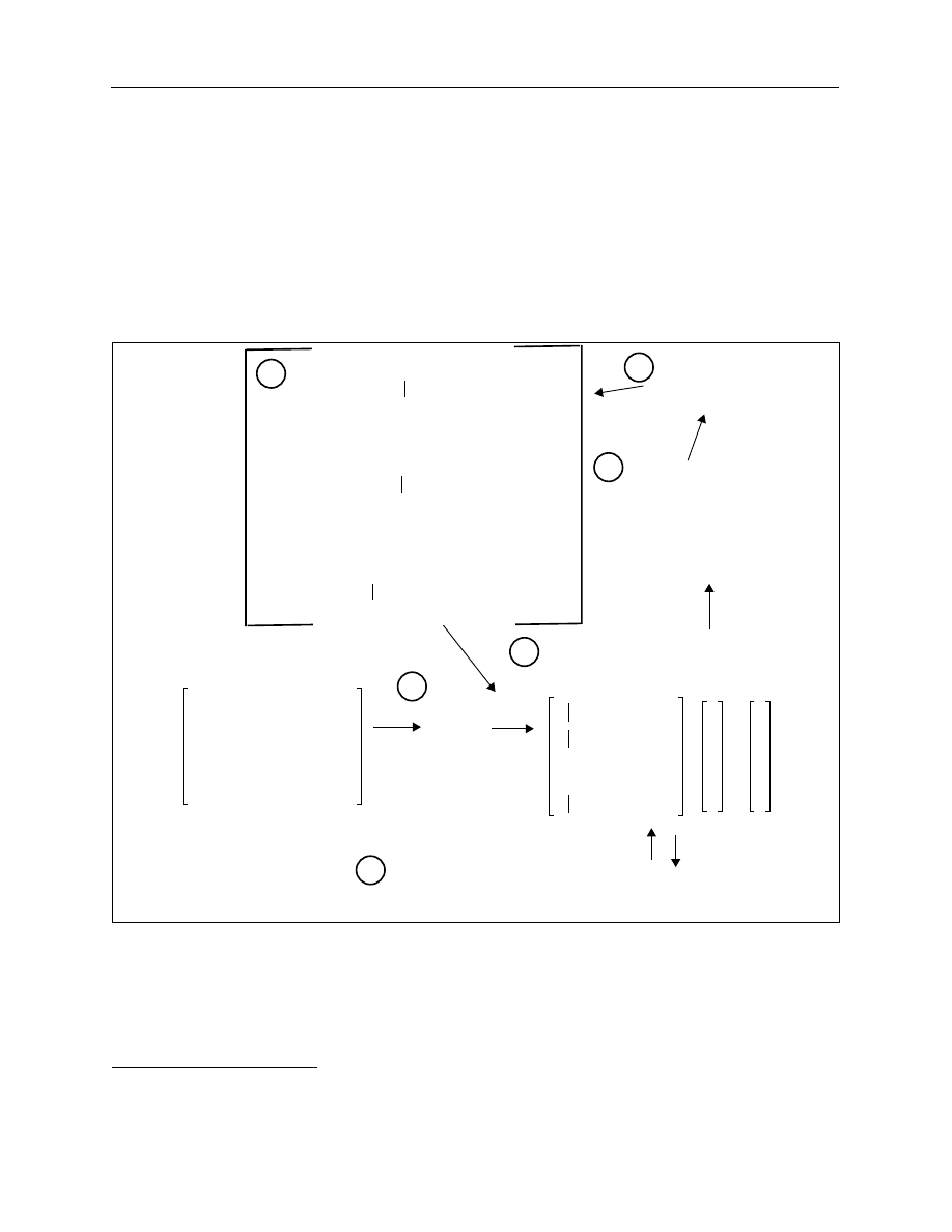
forward interest rate values. Figure 2 details the previously outlined process following the steps
from A to F.
Figure 2. Steps in the estimation of Nelson-Siegel and Svensson models
As indicated, the process describes the minimization of price errors rather than YTM
errors. Price errors were selected because the yield calculations necessary to minimize YTM
errors are prohibitively time consuming in an iterative optimization framework. In contrast to the
9.
In particular, the
β
0
and
τ
1
values are forced to take positive values and the humps are restricted to fall between 0
and 30 years, which corresponds to the estimation range.
Instantaneous forward rate
function
f TT M
t
β
o
β
1
β
2
β
3
τ
1
τ
2
,
,
,
,
,
(
)
Zero-coupon rate
function
z TT M
t
β
o
β
1
β
2
β
3
τ
1
τ
2
,
,
,
,
,
(
)
Discount rate
function
disc TT M
t
β
o
β
1
β
2
β
3
τ
1
τ
2
,
,
,
,
,
(
)
Matrix of bond cash flows
(CF)
BON D
1
BON D
2
…
…
BON D
n
CF
1 1
,
CF
1 2
,
…
CF
1 m
,
CF
2 1
,
…
…
…
…
…
…
…
…
…
…
…
CF
n 1
,
…
…
CF
n m
,
Discount
matrix of
bond cash
flows using
the discount
rate function
Vector of theoretical bond prices -
observed prices = price errors
P
ˆ
1
β
o
β
1
β
2
β
3
τ
1
τ
2
,
,
,
,
,
(
)
P
ˆ
2
β
o
β
1
β
2
β
3
τ
1
τ
2
,
,
,
,
,
(
)
…
…
P
ˆ
n
β
o
β
1
β
2
β
3
τ
1
τ
2
,
,
,
,
,
(
)
P
1
P
2
…
…
P
n
–
ε
1
ε
2
…
…
ε
n
=
Numerical optimization:
Each time the value of the
parameters is changed, this
process is repeated. The
final parameters selected are
those that minimize the
selected objective function.
Decision variable: Log-likelihood approach or sum of squared price
errors with penalty parameter
Parameters
β
o
β
1
β
2
β
3
τ
1
τ
2
,
,
,
,
,
A
B
C
D
E
F

11
calculation of the bond price, each YTM calculation relies on a time-consuming numerical
approximation procedure.
10
It is nevertheless critical that the model be capable of consistently fitting the YTMs of the
full sample of bonds used in the estimation. The intention is to model the yield curve, not the price
curve. Focusing on price errors to obtain YTMs can create difficulties. As a result, an important
element in the optimization is the weighting of price errors, a procedure necessary to correct for
the heteroskedasticity that occurs in the price errors. To understand how this is problematic, one
needs to consider the relationship between yield, price, and the term to maturity of a bond. This
relationship is best explained by the concept of duration.
11
A given change in yield leads to a
much smaller change in the price of a 1-year treasury bill than a 30-year long bond. The corollary
of this statement is that a large price change for a 30-year long bond may lead to an identical
change in yield when compared to a much smaller price change in a 1-year treasury bill. The opti-
mization technique that seeks to minimize price errors will therefore tend to try to reduce the het-
eroskedastic nature of the errors by overfitting the long-term bond prices at the expense of the
short-term prices. This in turn leads to the overfitting of long-term yields relative to short-term
yields and a consequent underfitting of the short-end of the curve. In order to correct for this
problem, each price error is simply weighted by a value related to the inverse of its duration. The
general weighting for each individual bond has the following form:
12
where D
i
is the MacCauley duration of the ith bond.
13
(EQ 15)
There are a number of advantages of the Nelson-Siegel and Svensson approach compared
with the Super-Bell model:
•
The primary output of this model is a forward curve, which can be used as an
approximation of aggregate expectations for future interest rate movements.
10. Moreover, the time required for the calculation is an increasing function of the term to maturity of the underlying
bond. In addition, the standard Canadian yield calculations, particularly as they relate to accrued interest, are
somewhat complicated and would require additional programming that would serve only to lengthen the price-
to-yield calculation.
11. See Technical Appendix, Section A.3 on page 42 for more on the concept of duration.
12. The specifics of the weighting function are described in the Technical Appendix, Section B, on page 43. Note
that this general case has been expanded to also permit altering the weighting of benchmark bond and/or treasury
bill price errors.
13. This is consistent with the Bliss (1991) approach.
ω
i
1 D
i
⁄
1 D
j
⁄
j
1
=
n
∑
-----------------------
=

12
•
This class of models focuses on the actual cash flows of the underlying securities rather
than using the yield-to-maturity measure, which is subject to a number of shortcomings.
14
•
The functional form of the Nelson-Siegel and Svensson models was created to be capable
of handling a variety of the shapes that are observed in the market.
•
These models provide continuous forward, zero-coupon, and discount rate functions,
which dramatically increase the ease with which cash flows can be discounted. They also
avoid the need to introduce other models for the interpolation between intermediate points.
Nevertheless, there are some criticisms of this class of term structure model. Firstly, there
is a general consensus that the parsimonious nature of these yield curve models, while useful for
gaining a sense of expectations, may not be particularly accurate for pricing securities.
15
The main criticism of the Nelson-Siegel and Svensson methodologies, however, is that
their parameters are more difficult to estimate relative to the Super-Bell model. These estimation
difficulties stem from a function that, while linear in the beta parameters, is non-linear in the taus.
Moreover, there appear to be multiple local minima (or maxima) in addition to a global minimum
(or global maximum). To attempt to obtain the global minimum, it is therefore necessary to
estimate the model for many different sets of starting values for the model parameters. Complete
certainty on the results would require consideration of virtually all sets of starting values over the
domain of the function; this is a very large undertaking considering the number of parameters.
With six parameters, all possible combinations of three different starting parameter values amount
to
different starting values, while five different starting values translate into
different sets of starting values. The time required to estimate the model, therefore,
acts as a constraint on the size of the grid that could be considered and hence the degree of pre-
cision that any estimation procedure can attain.
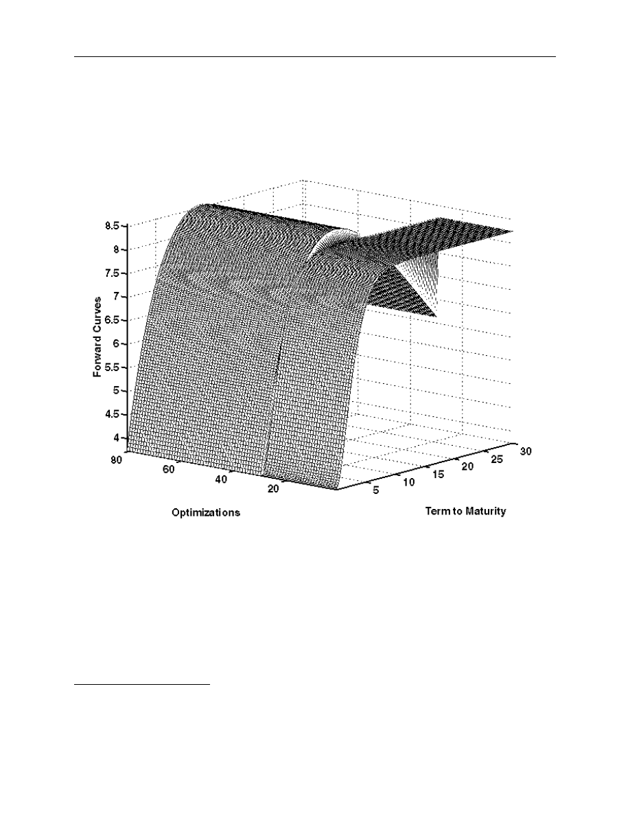
By way of example, Figures 3 and 4 demonstrate the sensitivity of the Nelson-Siegel and
Svensson models to the starting parameter values used for a more dramatic date in the sample,
17 January 1994. In Figure 3, only 29 of the 81 sets of starting values of the parameters for the
Nelson-Siegel model on that date give a forward curve close to the best one estimated within this
14. See Technical Appendix, Section A.2, “Yield to maturity and the ‘coupon effect’,” page 40 for more details.
15. This is because, by the very nature as a “parsimonious” representation of the term structure, they fit the data less
accurately than some alternative models such as cubic splines.
3
6
729
=
5
6
15 625
,
=
13
model.
16
For the results of the Svensson model, presented in Figure 4, only 11 of the 256 sets of
starting parameters are close to the best curve.
Figure 3. Estimation of Nelson-Siegel forward curves for 17 January 1994
(81 different sets of starting parameters)
16. The definition of closeness to the best forward curve is based on estimated value for the objective function used
in the estimation. An estimated curve is close to the best one when its estimated objective function value is at less
than 0.1 per cent of the value of the highest objective function calculated. For further details on the objective
functions used, see Technical Appendix, Section D, “Mechanics of the estimation,” on page 46.
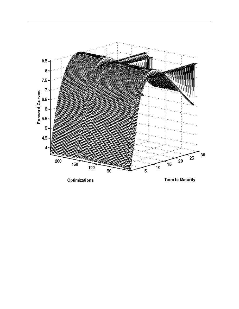
14
Figure 4. Estimation of Svensson forward curves for 17 January 1994
(256 different sets of starting parameters)
In Section 4, the estimation issues are addressed directly by comparing the performance of
the Nelson-Siegel, the Svensson, and the Super-Bell yield curve models in terms of the goodness
of fit of the estimated curves to the Canadian data, the time required to obtain them, and their
robustness to different strategies of optimization.
3.
DATA
Prior to discussing the details of the various term structure models examined in this paper,
it is necessary to describe Government of Canada bond and treasury bill data. The following sec-
tions briefly describe these instruments and the issues they present for the modelling of the term
structure of interest rates.

15
3.1
Description of the Canadian data
The two fundamental types of Canadian-dollar-denominated marketable securities issued
by the Government of Canada are treasury bills and Canada bonds.
17
As of 31 August 1998, the
Government of Canada had Can$89.5 billion of treasury bills and approximately Can$296 billion
of Canada bonds outstanding. Together, these two instruments account for more than 85 per cent
of the market debt issued by the Canadian government.
18
Treasury bills, which do not pay periodic interest but rather are issued at a discount and
mature at their par value, are currently issued at 3-, 6-, and 12-month maturities. Issuance cur-
rently occurs through a biweekly “competitive yield” auction of all three maturities. The 6-month
and 1-year issues are each reopened once on an alternating 4-week cycle and ultimately become
fungible with the 3-month bill as they tend towards maturity. At any given time, therefore, there
are approximately 29 treasury bill maturities outstanding.
19
Due to limitations in data availability,
however, there is access only to 5 separate treasury bill yields on a consistent basis: the 1-month,
2-month, 3-month, 6-month, and 1-year maturities.
Government of Canada bonds pay a fixed semi-annual interest rate and have a fixed
maturity date. Issuance involves maturities across the yield curve with original terms to maturity
at issuance of 2, 5, 10, and 30 years.
20
Each issue is reopened several times to improve liquidity
and achieve “benchmark status.”
21
Canada bonds are currently issued on a quarterly “competitive
yield” auction rotation with each maturity typically auctioned once per quarter.
22
In the interests
of promoting liquidity, Canada has set targets for the total amount of issuance to achieve
“benchmark status”; currently, these targets are Can$7 billion to Can$10 billion for each maturity.
The targets imply that issues are reopened over several quarters in order to attain the desired
liquidity.
17. See Branion (1995) for a review of the Government of Canada bond market, and Fettig (1994) for a review of the
treasury bill market.
18. The remaining market debt consists of Canada Saving Bonds, Real Return Bonds, and foreign currency
denominated debt.
19. Effective 18 September 1997, the issuance cycle was changed from a weekly to a biweekly auction schedule.
Previously, there were always at least 39 treasury bill maturities outstanding at any given time. The changes in
the treasury bill auction schedule were designed to increase the amount of supply for each maturity by reducing
the number of maturity dates that exist for treasury bills.
20. Canada eliminated 3-year bond issues in early 1997; the final 3-year issue was 15 January 1997.
21. A “benchmark” bond is analogous to an “on-the-run” U.S. Treasury security in that it is the most actively traded
security for a given maturity.
22. It is important to note that Government of Canada bond yields are quoted on an Actual/Actual day count basis
net of accrued interest. The accrued interest, however, is by market convention calculated on an Actual/365 day
count basis. See Barker (1996) and Kiff (1996).

16
At any given time, therefore, there are at least four benchmark bonds outstanding with
terms to maturity of approximately 2, 5, 10, and 30 years.
23
These bonds are the most actively
traded in the Canadian marketplace. They are also often subject to underpricing in comparison
with other Canada bonds because of a stronger demand. It could then be argued that these bonds
should be excluded from the sample to avoid any downward bias in the estimation of the Canadian
yield curve. Nevertheless, given that the Bank’s main interest in estimating yield curves is to
provide insights into the evolution of market expectations, it is considered essential that the infor-
mation contained in these bonds be incorporated into the yield curve estimation. Therefore, all the
benchmark bonds are forced to appear in all data sets.
Historically, the Government of Canada has also issued bonds with additional features on
top of the “plain vanilla” structure just described. Canada has in the past issued bonds with cal-
lable and extendible features and a small number of these bonds remain outstanding. In addition,
“purchase fund” bonds, which require periodic partial redemptions prior to maturity, were also
issued in the 1970s. Finally, Real Return Bonds (RRB), which pay a coupon adjusted for changes
in the Canadian consumer price index, were introduced in December 1991. There are two RRB
maturities outstanding for a total of approximately Can$10 billion.
24
These bonds with unique
features—purchase fund bonds and RRB—are flagged in the data base and subsequently excluded
from the data set. Real Return Bonds are also excluded as their yields, which are quoted on a real
rather than a nominal basis, are not directly comparable with nominal yields.
25
3.2
Why are the data important?
The only bonds selected from the universe of Government of Canada bond and treasury
bill data are those that are indicative of current market yields. This is because, regardless of the
type of model selected, the results of a given yield curve model depend importantly on the data
used to generate it. The examination of different filterings is therefore essential to provide confi-
dence in the choice of the model and to ensure its efficient application. As a result, a system of
filters is used to omit bonds that create distortions in the estimation of the yield curve. Analysis is
centred on two specific aspects of data filtering that are considered strategic: the severity of the fil-
tering (or its “tightness”), and the treatment of securities at the short-end of the term structure.
The severity of filtering includes filters dealing with the maximum divergence from par value and
the minimum amount outstanding required for the inclusion of a bond. The short-end of the term
structure involves questions surrounding the inclusion or exclusion of treasury bills and bonds
23. As previously discussed, new issues may require two or more reopenings to attain “benchmark status.” As a
result, the decision as to whether or not a bond is a benchmark is occasionally a matter of judgment. This could
lead to situations where more than one benchmark may exist for a given maturity.
24. See Côté, Jacob, Nelmes, and Whittingham (1996) for a discussion of the Canadian Real Return Bond.
25. There are approximately nine bonds with special features in the government’s portfolio.

17
with short term to maturities. The two main filtering categories are considered in the following
discussion.
3.3
Approaches to the filtering of data
3.3.1 Severity of data filtering: Divergence from par and amount outstanding
At present, there are 81 Canada bonds outstanding. This translates into an average issue
size of roughly Can$3.5 billion. In reality, however, the amount outstanding of these bonds varies
widely from Can$100 million to Can$200 million to just over Can$10 billion. Outstanding bonds
of relatively small size relate to the previous practice of opening a new maturity for a given bond
when the secondary market yield levels for the bond differed from the bond’s coupon by more
than 50 basis points. This is no longer the practice, given the benchmark program. At present, the
current maturity is continued until the benchmark target sizes are attained irrespective of whether
the reopening occurs at a premium or a discount. As bonds should have the requisite degree of
liquidity to be considered, bonds with less than a certain amount outstanding should be excluded
from the data set.
26
A relatively small value is assigned to the “minimum amount outstanding”
filter in order to keep as many bonds as possible in the sample. One could argue, however, that
only bonds with greater liquidity should be kept in the sample. This is an issue that will be inves-
tigated in the analysis of the data problem.
27
The term “divergence from par value” is used to describe the possible tax consequences of
bonds that trade at large premiums or discounts to their par value. Under Canadian tax legislation,
interest on bonds is 100 per cent taxable in the year received, whereas the accretion of the bond’s
discount to its par value is treated as a capital gain and is only 75 per cent taxable and payable at
maturity or disposition (whichever occurs first). As a result, the purchase of a bond at a large dis-
count is more attractive, given these opportunities for both tax reduction and tax deferral. The
willingness of investors to pay more for this bond, given this feature, can lead to price distortions.
To avoid potential price distortions when large deviations from par exist, those bonds that trade
more than a specified number of basis points at a premium or a discount from their coupon rate
should be excluded.
28
The number of basis points selected should reflect a threshold at which the
tax effect of a discount or premium is believed to have an economic impact.
29
The tax impact is
26. For example, if the specified minimum amount outstanding is Can$500 million, no bonds would be excluded on
15 June 1989 and eight bonds on 15 July 1998.
27. Of note, the amount outstanding of each individual issue could not be considered before January 1993 because of
data constraints.
28. If this filter were set at 500 basis points, 8 bonds would be excluded on 15 June 1989 and 26 bonds on 15 July
1998.
29. See Litzenberger and Rolfo (1984).

18
somewhat mitigated in the Canadian market, however, as the majority of financial institutions
mark their bond portfolios to market on a frequent basis. In this case, changes in market valuation
become fully taxable immediately, thereby reducing these tax advantages somewhat. Moreover,
some financial institutions are not concerned by these tax advantages.
30
The divergence from par value and the amount outstanding filters are intimately related
because bonds that trade at large discounts or premiums were typically issued with small amounts
outstanding during transition periods in interest rate levels. Consequently, any evaluation or
testing of this filter must be considered jointly with the minimum amount outstanding tolerated.
These two filtering issues combined can then be identified as the severity or tightness of the fil-
tering constraints. A looser set of divergence from par value and amount outstanding filtering cri-
teria should provide robustness in estimation but can introduce unrepresentative data to the
sample. Conversely, more stringent filtering criteria provide a higher quality of data but can lead
to poor results given its sparsity. Specifically, tighter filtering reduces the number of observations
and can make estimation difficult given the dispersion of the data. To cope with this data problem,
the empirical analysis will include an evaluation of the sensitivity of the models’ results to the
degree of tightness chosen for these two filters.
3.3.2 The short-end: Treasury bills and short-term bonds
Choosing the appropriate data for modelling the short-end of the curve is difficult. Canada
bonds with short terms to maturity (i.e., roughly less than two years) often trade at yields that
differ substantially from treasury bills with comparable maturities.
31
This is largely due to the sig-
nificant stripping of many of these bonds, which were initially issued as 10- or 20-year bonds with
relatively high coupons leading to substantial liquidity differences between short-term bonds and
treasury bills.
32
From a market perspective, these bond observations are somewhat problematic
due to their heterogeneity in terms of coupons (with the associated coupon effects) and liquidity
levels.
As a result of these liquidity concerns, one may argue for the inclusion of treasury bills in
the estimation of the yield curve to ensure the use of market rates for which there is a relatively
30. For example, earnings of pension funds on behalf of their beneficiaries are taxable only at withdrawal from the
pension accounts. Therefore, most investment managers of pension funds are indifferent to any tax advantage.
31. See Kamara (1990) for a discussion of differences in liquidity between U.S. Treasury bills and U.S. Treasury
bonds with the same term to maturity.
32. In 1993, reconstitution of Government of Canada strip bonds was made possible in combination with the
introduction of coupon payment fungibility. At that point in time, a number of long-dated high-coupon bonds
were trading at substantial discounts to their theoretical value. The change in stripping practices played a
substantial role in permitting the market to arbitrage these differences. See Bolder and Boisvert (1998) for more
information on the Government of Canada strip market.

19
high degree of confidence. Treasury bills are more uniform, more liquid, and do not have a
coupon effect given their zero-coupon nature. The question arises as to whether or not to use
short-term bonds and/or treasury bills in the data sample. Using only treasury bills would avoid
the estimation problems related to the overwhelming heterogeneity of coupon bonds at the short-
end of the maturity spectrum and anchor the short-end of the yield curves by the only zero-coupon
rates that are observed in the Canadian market.
Recent changes in the treasury bill market have nonetheless complicated data concerns at
the short-end of the curve. Declining fiscal financial requirements have led to sizable reductions in
the amount of treasury bills outstanding. In particular, the stock of treasury bills has fallen from
$152 billion as at 30 September 1996 to $89.5 billion as at 31 August 1998. This reduction in
stock with no corresponding reduction in demand has put downward pressure on treasury bill
yields.
33
This raises concerns about the use of treasury bills in the data sample. This data problem
will also be addressed in the empirical analysis, by an estimation of the sensitivity of the models’
results to the type of data used to model the short-end of the maturity spectrum.
4.
EMPIRICAL RESULTS
To perform an empirical analysis of the behaviour of the different yield curve models and
their sensitivity to data filtering conditions, a sample of 30 dates has been chosen, spanning the
last 10 years. The dates were selected to include 10 observations from an upward-sloping, a flat,
and an inverted term structure environment. This helps to give an understanding of how the model
performs under different yield curve slopes. The following table (Table 1) outlines the various
dates selected. It is worth noting that these dates could not be randomly selected as there are only
a few instances in the last 10 years of flat or inverted Canadian term structure environments. As a
result, the flat and inverted term structure examples are clustered around certain periods.
33. See Boisvert and Harvey (1998) for a review of recent developments in the Government of Canada on the
treasury bill market.

20
Table 1. Dates selected for estimation from different term structure environments
As discussed in Section 3.3, there is a wide range of possible data filtering combinations
that could be analyzed and their interaction is complex. As a result, examination has been limited
to a few dimensions. To do so, first a “benchmark” filtering case is defined, based on a set of pre-
liminary choices for each type of filtering criteria. The benchmark case is summarized as follows:
Table 2. Filter settings for the benchmark case
This benchmark data filtering case is held constant for a variety of different estimation
approaches (detailed in Section 4.1) and deals explicitly with the estimation problem. After this
analysis is complete, the best optimization approach is selected and used to consider three alter-
native data filtering scenarios. Each of these alternatives is contrasted in Section 4.2 with the
benchmark case to examine the models’ sensitivity to the two main aspects that were discussed in
the previous section. Thus the estimation problem is considered while holding constant the data
issue, and the data problem is subsequently examined holding the estimation problem constant.
4.1
The “estimation problem”
As illustrated in Section 2.2, the Nelson-Siegel and Svensson models are sensitive to the
estimation procedure chosen and particularly to the starting values used for the parameters.
Moreover, the time required to increase the robustness of an estimated curve, or the confidence of
Positively sloped
term structure
Flat term structure
Inverted term
structure
15 February 1993
15 August 1988
15 January 1990
15 July 1993
18 August 1988
15 May 1990
17 January 1994
23 August 1988
15 August 1990
16 May 1994
29 August 1988
13 December 1990
15 August 1994
15 February 1991
14 April 1989
15 February 1995
25 February 1991
15 June 1989
17 July 1995
4 March 1991
15 August 1989
15 February 1996
11 March 1991
16 October 1989
15 August 1996
15 June 1998
15 December 1989
16 December 1996
15 July 1998
15 March 1990
Type of data filter
Filter setting
Minimum amount outstanding
Can$500 million
Divergence from par: | Coupon - YTM |
500 basis points
Inclusion of treasury bills
Yes
Inclusion of bonds with less than 2 years TTM
No

21
having a global minimum, increases exponentially with the number of different starting values
chosen for each parameter. To address this problem of estimation, a number of procedures are
examined to find a reasonable solution to this trade-off between time, robustness, and accuracy.
Specifically, the strategy for dealing with the estimation problem was to consider a number of dif-
ferent approaches to the problem for the 30 different dates chosen and to examine the results using
the benchmark selection of the data. The Nelson-Siegel and Svensson curves are not determined
in a statistical estimation but rather in a pure optimization framework. Therefore, an objective
function must be specified and subsequently minimized (or maximized), using a numerical opti-
mization procedure. Consequently, the approaches differ in terms of the formulation of the
objective function and the details of the optimization algorithm.
Two alternative specifications of the objective function are examined. Both approaches
seek to use the information in the bid-offer spread. One uses a log-likelihood specification while
the other minimizes a special case of the weighted sum of squared price errors. The log-like-
lihood formulation replaces the standard deviation in the log-likelihood function with the bid-
offer spread from each individual bond. The sum of squared price error measure puts a reduced
weight on errors occurring inside the bid-offer spread but includes a penalty for those observa-
tions occurring outside the bid-offer spread. These two formulations are outlined in greater detail
in the Technical Appendix.
Each optimization algorithm can be conceptually separated into two parts: the global and
local search components. The global search is defined as the algorithm used to find the appro-
priate region over the domain of the objective function. The distinction is necessary due to the
widely varying parameter estimates received for different set of starting values. The intent is to
broadly determine a wide range of starting values over the domain of the function and then run the
local search algorithm at each of these points. The local search algorithm finds the solution from
each set of starting values using either Sequential Quadratic Programming (a gradient-based
method) and/or the Nelder and Meade Simplex Method (a direct search, function-evaluation-
based method). Two basic global search algorithms are used:
•
Full estimation (or “coarse” grid search): This approach uses a number of different sets
of starting values and runs a local search for each set and then selects the best solution. In
both the Nelson-Siegel and Svensson models, the
β
0
and
β
1
parameters were not varied but
rather set to the long-run term to maturity and the difference between the longest and
shortest yield to maturity. In the Nelson-Siegel model, therefore, 9 combinations of the
remaining 2 parameters (
β
2
and
τ
1
) are used in the grid for a total of 81 sets of starting
parameters. In the Svensson model, there are 4 combinations of 4 parameters (
β
2
, β
3
, τ
1
,
τ
2
) for a total of 256 starting values. In the full-estimation algorithm, the Sequential

22
Quadratic Programming (SQP) algorithm is used; this is replaced by the Simplex method
when the SQP algorithm fails to converge.
34
•
Partial estimation: The second approach uses partial estimation of the parameters.
Specifically, this global search algorithm divides the parameters into two groups, the
β
s (or
linear parameters) and the
τ
s (or the non-linear parameters). The algorithm works in a
number of steps where one group of parameters is fixed while the other is estimated.
35
The
full details of this algorithm are presented in the Technical Appendix, Section E.2, “Partial-
estimation algorithm,” on page 52.
In total, four separate approaches to parameter estimation are examined for each of the
two parametric models: two separate formulations of the objective function and two separate
global search algorithms. The estimation of the parameters for the Super-Bell model is a simple
matter of OLS regression. This means that, while there are only three models from which to
select, there is a total of nine sets of results (this is depicted graphically in Figure 5).
Figure 5. The analysis of the “estimation problem”
The use of a numerical optimization procedure neither provides standard error measures
for parameter values nor permits formal hypothesis testing. Instead, therefore, the approach
involves a comparison among a variety of summary statistics. Three main categories of criteria
have been selected: goodness of fit, speed of estimation, and robustness of the solution. A number
34. This idea comes from Ricart and Sicsic (1995) although they actually impose these as constraints. In this paper,
they are used as starting points. See Technical Appendix, Section E.1, “Full-estimation algorithm,” on page 50
for more detail.
35. In the partial-estimation algorithm, the SQP algorithm is used exclusively because there were no convergence
problems when estimating a smaller subset of parameters.
Model:
Log-likelihood
SSE with penalty
Full-estimation
Partial-estimation
objective function
parameter objective
function
algorithm
algorithm
Full-estimation
algorithm
Partial-estimation
algorithm
Nelson and
Siegel or
Svensson
Model
There are nine separate scenarios. Four approaches for
each parametric model and one for the Super-Bell model.

23
of different statistics were selected to assess the performance of each of the approaches under
each of these categories. The following sections discuss and present each group of criteria in turn.
4.1.1 Robustness of solution
Robustness of solution can be defined as how certain one is that the final solution is
actually the global minimum or maximum. This measurement criterion is examined first because
it provides an understanding of the differences and similarities between the optimization strat-
egies. Two measures of robustness are considered.
The first measure, in Table 3, compares the best objective function values for each of the
alternative optimization approaches. Only objective function values based on the same model
with the same estimation algorithm are directly comparable (i.e., one compares the figures in
Table 3 vertically rather than horizontally). Consequently, Table 3 compares the full- and partial-
estimation algorithms for each formulation of the objective function. A number of observations
follow:
•
In all cases, save one, the Nelson-Siegel partial- and full-estimation algorithms lead to the
same results. The one exception is the full-estimation algorithm, which provides a superior
value for the sum of squared errors objective function on 18 August 1988.
•
The Svensson model full-estimation algorithm provides in all cases a superior or identical
result to the partial-estimation algorithm. The full-estimation algorithm outperforms the
partial on eight occasions for the log-likelihood objective function and on seven occasions
for the sum of squared errors objective function.
•
The magnitude of a superior objective function value is also important. In aggregate, the
differences in objective function are quite small and it will be important to look to other
statistics to see the practical differences (particularly the goodness of fit) in the results of
these different solutions.

24
Table 3. Best objective function value
The second statistic to consider is the number of solutions in the global search algorithm
that converge to within a very close tolerance (0.01 per cent) of the best solution. Table 4 outlines
the aggregate results.
•
This is a rather imperfect measure for comparison among global search algorithms because
the partial estimation fixes sets of parameters, which necessarily constrain it from the
optimal solution. It is nonetheless useful for comparison between different specifications of
the objective function, between different models, and between different term structure
environments.
•
A not-surprising result is that the simpler Nelson-Siegel model has a much higher rate of
similar solutions (approximately 60 per cent for the full estimation versus approximately
30 per cent for the Svensson model).
•
It appears more difficult to estimate an upward-sloping term structure than one that is flat
or inverted. For the full-estimation algorithm, the flat and inverted term structures have
roughly twice as many similar solutions as in the upward-sloping yield curve environment.
•
The data do not suggest a substantial difference between the two alternative formulations
of the objective function.
Dates
Nelson-Siegel model
Svensson model
Nelson-Siegel model
Svensson model
Super-
Bell
model
OLS
estimation
Full-
estimation
algorithm
Partial-
estimation
algorithm
Full-
estimation
algorithm
Partial-
estimation
algorithm
Full-
estimation
algorithm
Partial-
estimation
algorithm
Full-
estimation
algorithm
Partial-
estimation
algorithm
Log-likelihood objective function
Sum of squared errors objective function
Normal
100,707.6
100,707.6
86,799.7
87,755.1
51,813.5
51,813.5
23,997.7
25,908.4
n/a
Flat
61,707.3
61,707.3
54,616.2
54,837.2
97,587.4
97,743.8
83,405.1
83,643.4
n/a
Inverted
24,006.0
24,006.0
21,016.5
21,432.2
40,660.5
40,660.5
34,681.5
35,182.6
n/a
Total
62,140.3
62,140.3
54,144.1
54,674.8
63,353.8
63,406.0
47,361.5
48,244.8
n/a

25
Table 4. Percentage of solutions in global search within 0.01 per cent of best solution
4.1.2 Goodness of fit
This is arguably the most important of the three criteria because these measures indicate
how well the model and its associated estimation procedure describe the underlying data. It
should be stated at the beginning that, in those instances in the previous section, particularly for
the Nelson-Siegel model where the solutions were identical, the results will be identical. This
section will therefore focus on the differences between models, objective functions, and optimi-
zation strategy where appropriate. Five different measures have been selected to determine the
“fit” of the various strategies. The measures focus on yield errors. This is important because,
although price is used in the estimation of the models, it is appropriately weighted to ensure a
good fit to the bond yield to maturity.
Table 5 displays the first measure of goodness of fit, the yield root mean square error
(RMSE
yield
).
36
In a general sense, this measure can be interpreted as the standard deviation of the
yield errors.
•
In aggregate, the Svensson model appears to perform about one basis point better than the
Nelson-Siegel model.
•
The data also suggest that all the models do a superior job of fitting an upward-sloping term
structure relative to their flat or inverted counterparts. Caution is suggested in this
assessment, given the relatively skewed nature of the sample selection. There may be
reason to suspect that the periods from which the inverted and flat term structure dates were
selected are different from the broader range of dates selected for the upward-sloping term
structure.
Dates
Nelson-Siegel model
Svensson model
Nelson-Siegel model
Svensson model
Super-
Bell
model
OLS
estimation
Full-
estimation
algorithm
Partial-
estimation
algorithm
Full-
estimation
algorithm
Partial-
estimation
algorithm
Full-
estimation
algorithm
Partial-
estimation
algorithm
Full-
estimation
algorithm
Partial-
estimation
algorithm
Log-likelihood objective function
Sum of squared errors objective function
Normal
58.8%
10.0%
17.1%
6.1%
58.6%
5.7%
16.8%
1.8%
n/a
Flat
53.1%
17.3%
35.8%
5.4%
52.5%
1.3%
35.1%
8.9%
n/a
Inverted
76.8%
23.0%
35.1%
9.8%
76.3%
34.0%
32.9%
2.4%
n/a
Total
62.8%
16.8%
29.3%
7.1%
62.5%
17.5%
28.2%
4.4%
n/a
36. The root mean square error is defined as
.
RMSE
yield
e
i yield
,
e
yield
–
(
)
2
n
--------------------------------------------
i
1
=
N
∑
=

26
•
Despite the differences in the solutions between the full- and partial-estimation algorithm
of the Svensson model, the results are quite similar. Indeed, the full-estimation algorithm
provides an improvement of only one-tenth of a basis point over the partial estimations.
This would suggest that the practical differences among the solutions are not large.
•
Note that the Svensson and Nelson-Siegel models provide a marked improvement relative
to the Super-Bell model in the upward-sloping and inverted term structure environments
but are roughly similar when the term structure is flat.
Table 5. Root mean square yield error (in basis points)
The RMSE
yield
measure is essentially a standard-deviation-based measure that uses the
squared deviations from the mean as its numerator. As a consequence, it is rather sensitive to out-
liers. For this reason, an alternative measure of yield errors is also examined: the average absolute
value of yield errors (AABSE
yield
).
37
This measure is less sensitive to extreme points. The results
of this measure are illustrated in Table 6.
•
Given the reduced sensitivity to large values, it is hardly surprising to note that the errors
are in general somewhat smaller (roughly about five basis points for the total sample). The
fact that the differences between RMSE
yield
and the AABSE
yield
are larger for the flat and
inverted dates than for the normal dates suggests that there are more outliers occurring on
these dates.
•
In general, however, the same relationships that appear in the RMSE
yield
are evident in
these results. That is, the Svensson model slightly outperforms the Nelson-Siegel model
and the upward-sloping term structure is a better fit than the flat and inverted yield curve
environments.
Dates
Nelson-Siegel model
Svensson model
Nelson-Siegel model
Svensson model
Super-
Bell
model
OLS
estimation
Full-
estimation
algorithm
Partial-
estimation
algorithm
Full-
estimation
algorithm
Partial-
estimation
algorithm
Full-
estimation
algorithm
Partial-
estimation
algorithm
Full-
estimation
algorithm
Partial-
estimation
algorithm
Log-likelihood objective function
Sum of squared errors objective function
Normal
8.6
8.6
6.5
6.5
8.8
8.6
6.5
6.5
11.3
Flat
25.5
25.5
24.4
25.0
25.5
25.5
24.4
24.9
25.7
Inverted
18.1
18.1
18.5
18.5
18.1
18.1
18.5
18.5
26.2
Total
17.4
17.4
16.5
16.7
17.4
17.4
16.5
16.6
21.1
37. The average absolute value of yield errors is defined as:
.
AABSE
yield
e
i yield
,
e
yield
–
n
---------------------------------------
i
1
=
N
∑
=

27
•
It is interesting to note that the Svensson model full-estimation algorithm fits marginally
less well relative to the partial-estimation algorithm (on a margin of one-tenth of one basis
point). This is the opposite of the results found using RMSE
yield
measure.
•
Again, both the Svensson and Nelson-Siegel models provide a substantially improved fit
over the Super-Bell model (on aggregate by three to four basis points) in upward-sloping
and inverted environments. All models appear to perform similarly in a flat term structure
setting.
Table 6. Average absolute value of yield errors (in basis points)
The next measure of goodness of fit is termed the hit ratio. This statistic describes the
number of bonds with an estimated price inside the bid-offer spread as a percentage of the total
number of bonds estimated. The intent of this measure is to get a sense of the number of bonds
that were essentially perfectly priced. This is particularly interesting when considering the formu-
lation of the objective function measures, which explicitly use the bid-offer spread. Table 7 illus-
trates the results.
•
The hit ratio is roughly two times higher for the upward-sloping relative to the flat and
inverted term structures. That is to say, approximately twice as many estimated bond yields
fall between the bid and offer spread for the upward-sloping term structure observations.
•
The Nelson-Siegel model appears to perform better than the Svensson model for the flat
and inverted term structures and worse for an upward-sloping yield curve. In aggregate,
they even out and show little difference.
•
Once again, in all cases, the Nelson-Siegel and Svensson models outperform the Super-
Bell model on this measure except for the flat term structure dates.
Dates
Nelson-Siegel model
Svensson model
Nelson-Siegel model
Svensson model
Super-
Bell
model
OLS
estimation
Full-
estimation
algorithm
Partial-
estimation
algorithm
Full-
estimation
algorithm
Partial-
estimation
algorithm
Full-
estimation
algorithm
Partial-
estimation
algorithm
Full-
estimation
algorithm
Partial-
estimation
algorithm
Log-likelihood objective function
Sum of squared errors objective function
Normal
6.6
6.6
5.1
5.0
6.6
6.6
5.1
5.0
9.5
Flat
17.4
17.4
16.4
16.8
17.4
17.5
16.4
16.7
17.0
Inverted
13.4
13.5
13.1
13.1
13.4
13.4
13.1
13.1
18.4
Total
12.5
12.5
11.5
11.6
12.5
12.5
11.5
11.6
15.0

28
Table 7. Hit ratio (estimated yield inside bid-offer spread/total bonds)
The following two tables, Tables 8 and 9, provide a sense of whether or not the estimates
are biased in one direction or another. These two measures, which are essentially rough measures
of dispersion, describe the percentage of estimated yields exceeding the bid yield and the per-
centage of estimated yields below the offer yield.
•
The Super-Bell model tends to overestimate yields to maturity or, alternatively, to
underestimate bond prices.
•
For upward-sloping yield curves, the Nelson-Siegel model tends to underestimate the
actual yields to maturity, while the Svensson model does not seems to be biased in a
direction.
Table 8. Percentage of bonds with estimated yields exceeding the bid
•
For flat curves, both the parametric models tend to underestimate the actual yields to
maturity, while they seem to underestimate yields to maturity for inverted curves, although
by a lesser amount than the Super-Bell model.
•
In general, the Svensson model appears to perform slightly better than the Nelson-Siegel
model with less tendency to be biased in one direction.
Dates
Nelson-Siegel model
Svensson model
Nelson-Siegel model
Svensson model
Super-
Bell
model
OLS
estimation
Full-
estimation
algorithm
Partial-
estimation
algorithm
Full-
estimation
algorithm
Partial-
estimation
algorithm
Full-
estimation
algorithm
Partial-
estimation
algorithm
Full-
estimation
algorithm
Partial-
estimation
algorithm
Log-likelihood objective function
Sum of squared errors objective function
Normal
9.7%
9.7%
11.5%
11.5%
9.7%
9.7%
11.4%
11.5%
6.9%
Flat
4.3%
4.3%
3.4%
3.2%
4.3%
4.2%
3.7%
3.5%
3.8%
Inverted
5.0%
5.0%
3.8%
4.1%
5.0%
5.0%
4.0%
4.2%
2.1%
Total
6.3%
6.3%
6.3%
6.3%
6.3%
6.3%
6.3%
6.4%
4.3%
Dates
Nelson-Siegel model
Svensson model
Nelson-Siegel model
Svensson model
Super-
Bell
model
OLS
estimation
Full-
estimation
algorithm
Partial-
estimation
algorithm
Full-
estimation
algorithm
Partial-
estimation
algorithm
Full-
estimation
algorithm
Partial-
estimation
algorithm
Full-
estimation
algorithm
Partial-
estimation
algorithm
Log-likelihood objective function
Sum of squared errors objective function
Normal
47.0%
47.0%
50.0%
48.4%
47.0%
47.0%
50.2%
48.7%
55.8%
Flat
47.5%
47.5%
46.5%
46.9%
47.5%
47.9%
46.6%
47.0%
52.5%
Inverted
56.3%
56.3%
53.2%
53.5%
56.3%
56.3%
53.2%
53.7%
60.8%
Total
50.3%
50.3%
50.0%
49.6%
50.3%
50.4%
50.0%
49.8%
56.4%

29
Table 9. Percentage of bonds with estimated yields below the offer
4.1.3 Speed of estimation
The final criterion, the speed of optimization, is one of large practical importance. Given
the finite amount of time and computing resources available to solve this problem, a fair amount
of importance will be placed on this criterion.
38
The first measure examined is the average amount of time required for each individual
local search within the larger global search algorithm. The full- and partial-estimation algorithms
cannot be explicitly compared, given that full estimation has a much harder task (for each indi-
vidual iteration) relative to the partial-estimation approach. It nevertheless provides some inter-
esting information regarding the differences between the two techniques. Table 10 details this
measure.
•
The full-estimation algorithm, for both models and objective function values, appears to
take on average 10 times longer per iteration than the partial-estimation approach.
•
The Svensson model requires approximately four times as much time compared with the
Nelson-Siegel model for both objective function formulations and global estimation
algorithms.
•
It does not appear that there are substantial differences in the average amount of time
required per iteration for the different term structure environments.
•
The log-likelihood objective function is slightly faster (on the order of about one second)
for both the Nelson-Siegel and Svensson models.
Dates
Nelson-Siegel model
Svensson model
Nelson-Siegel model
Svensson model
Super-
Bell
model
OLS
estimation
Full-
estimation
algorithm
Partial-
estimation
algorithm
Full-
estimation
algorithm
Partial-
estimation
algorithm
Full-
estimation
algorithm
Partial-
estimation
algorithm
Full-
estimation
algorithm
Partial-
estimation
algorithm
Log-likelihood objective function
Sum of squared errors objective function
Normal
53.0%
53.0%
50.0%
51.6%
53.0%
53.0%
49.8%
51.3%
44.2%
Flat
52.5%
52.5%
53.5%
53.1%
52.5%
52.1%
53.4%
53.0%
47.5%
Inverted
43.7%
43.7%
46.8%
46.5%
43.7%
43.7%
46.8%
46.3%
39.2%
Total
49.7%
49.7%
50.0%
50.4%
49.7%
49.6%
50.0%
50.2%
43.6%
38. All the estimations were performed using a Sun Microsystems Ultra 10 workstation and the mathematical
software, Matlab.

30
Table 10. Average time per local search algorithm (in seconds)
Table 11 summarizes the final measure to be considered: the total amount of time per
global search. It is worth noting that, while this statistic gives a good approximation of the amount
of time required for the partial-estimation algorithm, it tends to underestimate the time required
for the full-estimation algorithm. Specifically, it has not been possible to capture the time required
by the SQP algorithm in those instances where the SQP algorithm did not converge and was
replaced by the Simplex algorithm.
•
In aggregate, the full estimations take roughly six times longer than the partial-estimation
algorithms.
•
As was the case with the previous measure, there do not appear to be substantial
differences in the time required for estimation of different term structure environments.
•
The log-likelihood and sum of squared error objective functions require approximately the
same amount of time for the full-estimation algorithm. The partial-estimation algorithm,
however, appears to be marginally faster (10 to 15 minutes) for the log-likelihood function.
Table 11. Total time for global search algorithm (in hours)
Dates
Nelson-Siegel model
Svensson model
Nelson-Siegel model
Svensson model
Super-
Bell
model
OLS
estimation
Full-
estimation
algorithm
Partial-
estimation
algorithm
Full-
estimation
algorithm
Partial-
estimation
algorithm
Full-
estimation
algorithm
Partial-
estimation
algorithm
Full-
estimation
algorithm
Partial-
estimation
algorithm
Log-likelihood objective function
Sum of squared errors objective function
Normal
11.3
1.7
47.5
4.1
11.5
1.6
48.5
4.4
0.5
Flat
10.7
2.0
49.0
4.6
11.1
2.2
50.3
6.2
0.5
Inverted
13.9
2.1
46.3
4.5
14.2
2.2
47.3
4.6
0.5
Total
12.0
1.9
47.6
4.4
12.3
2.0
48.7
5.1
0.5
Dates
Nelson-Siegel model
Svensson model
Nelson-Siegel model
Svensson model
Super-
Bell
model
OLS
estimation
Full-
estimation
algorithm
Partial-
estimation
algorithm
Full-
estimation
algorithm
Partial-
estimation
algorithm
Full-
estimation
algorithm
Partial-
estimation
algorithm
Full-
estimation
algorithm
Partial-
estimation
algorithm
Log-likelihood objective function
Sum of squared errors objective function
Normal
0.25
0.17
3.20
0.44
0.26
0.18
3.27
0.60
0.00013
Flat
0.24
0.37
3.31
0.54
0.25
0.30
3.40
0.88
0.00013
Inverted
0.31
0.47
3.13
0.66
0.32
0.43
3.20
0.71
0.00013
Total
0.27
0.33
3.21
0.55
0.28
0.30
3.29
0.73
0.00013

31
4.1.4 The “estimation” decision
As indicated, the final step in the “estimation problem” is to select the most promising
model and optimization strategy in order to examine two specific aspects of filtering the data. The
model ultimately selected was the Svensson model with a log-likelihood objective function using
the partial-estimation algorithm. There were several reasons for this decision:
•
Although the full-estimation procedure appears to provide slightly better solutions than the
partial-estimation algorithm, the resulting goodness-of-fit measures were not different in a
practical sense.
•
The full-estimation algorithm is prohibitively time consuming. On average, by
conservative measures, the full procedure required roughly six times longer than the
partial-estimation procedure.
•
There does not appear, in the statistics considered, to be much in the way of practical
difference between the two objective function formulations. As a result, the decision is
somewhat arbitrary. The log-likelihood specification was finally selected because it is
slightly faster for the partial-estimation algorithm.
4.2
The “data problem”
This section includes a sensitivity analysis of two aspects of data filtering that are con-
sidered important in the Canadian data: the severity of the filtering criteria, and the treatment of
the short-end of the term structure. Accordingly, the analysis performed in this section compares
the results obtained with the benchmark filtering relative to three alternative filtering settings: a
scenario with a more severe (or “tight”) setting, one with only bonds included at the short-end,
and one with both bonds and treasury bills at the short-end (see Figure 6). The settings for the
benchmark data filtering are outlined in Table 2. The different filtering is compared using the best
optimization approach from the previous section, that is, the Svensson yield curve with a log-like-
lihood objective function using the partial-estimation algorithm for the same 30 dates used in the
initial analysis.

32
Figure 6. The analysis of the “data problem”
To ensure the comparability among the different filtering settings and models, the same
summary statistics as those presented in the previous section are used: goodness of fit, robustness,
and speed of estimation. In addition, these statistics are calculated using the same unfiltered
observations as in the benchmark case, rather than the actual unfiltered observations of the various
alternative filterings.
The average number of unfiltered observations for each shape of curve for the different fil-
terings applied is listed in Table 12. The use of both bonds and bills at the short-end has the most
observations while the “tight” case, not surprisingly, has fewer observations relative to the alterna-
tives. The fact that there are more observations in the “bonds only” case suggests there are more
bonds at the short-end of the term structure than the five treasury bill observations used in the
benchmark case.
Table 12. Number of observations used in estimation (unfiltered observations)
Dates
a
a. Of note, the average number of available observations for normal, flat, and inverted curves is 95.8,
119.4, and 125.8 respectively, for a total average of 113.7 observations.
Benchmark case
“Bonds and bills”
case
“Bonds only”
case
“Tight” case
Normal
52.3
61.2
56.2
26.2
Flat
74.5
94.2
89.2
56.5
Inverted
83.3
101.7
97.2
65.5
Total
70.0
85.7
80.9
49.4
Benchmark
Severity of data
Treatment of the
“Tight” case
filtering settings
short-end of term
structure
“Bonds only”
“Bonds and bills”
case
Uses more stringent settings
for amount outstanding and
divergence from par value
Uses both bonds and t-bills to
estimate short-end of curve
Uses only bonds to estimate
the short-end of curve
Note that all different settings are compared using the Svensson
model, the log-likelihood objective function, and the partial-
estimation algorithm.
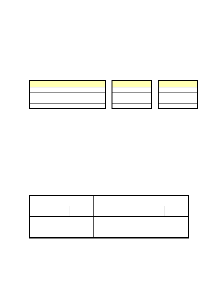
33
4.2.1 Tightness of data filtering
The first filtering issue deals with the severity of the filtering constraints. Given that the
benchmark case filtering settings are not particularly stringent, a more severe or “tight” set of fil-
tering criteria is analyzed (see Table 13). Note that the minimum amount outstanding has been
increased to $2.5 billion and the divergence from par value to 250 basis points. While these set-
tings are clearly debatable, they do represent a substantial tightening from the benchmark case.
Table 13. Filter settings: “Tight” case
Table 14 illustrates the summary statistics for the goodness of fit. The following observa-
tions are made:
•
The tight filtering tends to outperform the benchmark case filtering for the RMSE
yield
and
AABSE
yield
measures in flat or inverted term structures although they are broadly similar in
an upward-sloping environment.
•
When considering the hit ratio, however, there does not appear to be a significant difference
between the two filtering options.
•
The benchmark case filtering performs marginally better for upward-sloping yield curves.
Table 14. Goodness of fit: “Tight” vs. benchmark
Type of data filter
“Tight” filtering
“Benchmark” filtering
Minimum amount outstanding
Can$2,500 million
Can$500 million
Divergence from par: | Coupon - YTM |
250 basis points
500 basis points
Inclusion of treasury bills
Yes
Yes
Inclusion of bonds with less than 2 years TTM
No
No
Dates
Yield root mean square error
(in basis points)
Average absolute value of
yield errors (in basis points)
Hit ratio (%)
Benchmark
filtering
Tight
filtering
Benchmark
filtering
Tight
filtering
Benchmark
filtering
Tight
filtering
Normal
6.5
6.9
5.0
5.4
11.5%
11.9%
Flat
25.0
19.6
16.8
13.7
3.2%
3.1%
Inverted
18.5
15.8
13.1
11.7
4.1%
5.4%
Total
16.7
14.1
11.6
10.2
6.3%
6.8%

34
By reviewing the statistics on the speed of estimation (presented in Table 15), the fol-
lowing conclusions can be made:
•
The average time taken per local search algorithm is generally very close for the two
alternatives.
•
Similarly, the total time used for the global search algorithm is broadly comparable for
both filterings. Nevertheless, the tight filtering takes slightly more time on flat curve
estimations while the benchmark filtering is somewhat slower on inverted curve
estimations.
Table 15. Speed of estimation: “Tight” vs. benchmark
Finally, the results of the robustness statistics, as illustrated in Table 16, are as follows:
•
On average, the tight filtering attains a superior objective function value relative to the
benchmark filtering. This confirms the generally better fit observed in the goodness-of-fit
statistics.
•
The percentage of estimated objective functions that are within 0.1 per cent of the best
value obtained is of similar magnitude in both filtering cases.
Table 16. Robustness: “Tight” vs. benchmark
Dates
Average time per local
search algorithm
(in seconds)
Total time for global search
algorithm
(in hours)
Benchmark
filtering
Tight
filtering
Benchmark
filtering
Tight
filtering
Normal
4.1
4.1
0.44
0.44
Flat
4.6
4.8
0.55
0.67
Inverted
4.5
4.5
0.66
0.60
Total
4.4
4.5
0.55
0.57
Dates
Best objective function
values
Percentage of solutions in
global search within 0.01% of
best solution
Benchmark
filtering
Tight
filtering
Benchmark
filtering
Tight
filtering
Normal
87,755.1
87,732.9
21.6%
20.2%
Flat
54,837.2
49,560.0
18.2%
17.9%
Inverted
21,432.2
20,352.3
31.3%
31.9%
Total
54,674.8
52,548.4
23.7%
23.3%
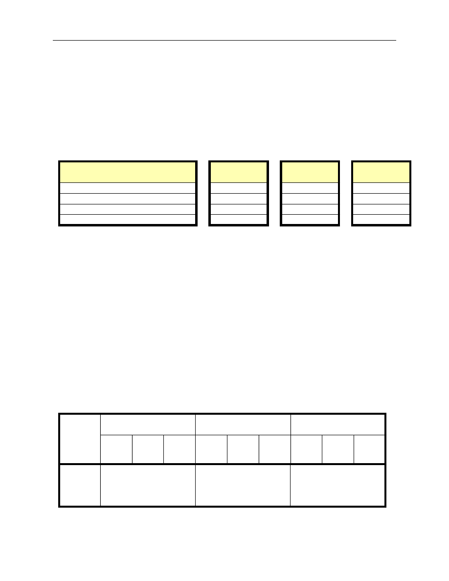
35
4.2.2 Data filtering at the short-end of the term structure
At the short-end of the curve, the data filtering question involves the inclusion of treasury
bills relative to the use of bond observations. To examine robustness of the model to the data
selected for this sector of the curve, three possible alternatives are considered: only treasury bills
(the benchmark case), only bonds, and both bonds and treasury bills. The two new alternatives—
termed “bonds only” and “bonds and bills”—have the following settings:
Table 17. Filter settings: “Bonds only” and “bonds and bills”
Comparing these two filtering alternatives to the benchmark case on the basis of goodness
of fit (see Table 18), it is observed that:
•
There is no clear winner among the two principal yield error measures. For upward-sloping
yield curves, there are smaller errors when both “bonds and bills” are used at the short-end
of the maturity spectrum. Benchmark filtering generally outperforms the two alternatives
for flat term structures. Finally, in an inverted environment, the benchmark case is superior
when considering the RMSE
yield
while the bond and bill case is the best when using
AABSE
yield
.The differences are nonetheless in most instances quite small.
•
The hit ratio appears to favour the benchmark filtering for upward-sloping curves. The
"bonds only" case is the clear winner in flat and inverted term structure environments.
Table 18. Goodness of fit: Short-end vs. benchmark
Type of data filter
“Bonds only”
filtering
“Bonds and
bills” filtering
“Benchmark”
filtering
Minimum amount outstanding
Can$500 million
Can$500 million
Can$500 million
Divergence from par: | Coupon - YTM |
500 basis points
500 basis points
500 basis points
Inclusion of treasury bills
No
Yes
Yes
Inclusion of bonds with less than 2 years TTM
Yes
Yes
No
Dates
Yield root mean square error
(in basis points)
Average absolute value of
yield errors (in basis points)
Hit ratio (%)
Bench-
mark
Bonds
only
Bonds
and
bills
Bench-
mark
Bonds
only
Bonds
and
bills
Bench-
mark
Bonds
only
Bonds
and
bills
Normal
6.5
6.8
6.4
5.0
5.3
4.8
11.5%
14.4%
14.0%
Flat
25.0
28.5
27.3
16.8
15.8
15.2
3.2%
7.8%
5.9%
Inverted
18.5
19.8
17.2
13.1
13.9
13.0
4.1%
6.0%
5.0%
Total
16.7
18.4
17.0
11.6
11.7
11.0
6.3%
9.4%
8.3%

36
The speed-of-estimation measures are detailed in Table 19.
•
The average time per local search algorithm is faster in all cases under the benchmark case.
•
This translates into a much lower total time of estimation for the benchmark filtering case
than for the other two alternatives. Notably, the estimations using only bonds at the short-
end of the maturity spectrum take twice as much time relative to the benchmark filtering.
Table 19. Speed of estimation: Short-end vs. benchmark
Table 20 details the robustness criteria.
•
Surprisingly, the best objective function values are the lowest for the "bonds and bills"
filtering and the highest for the benchmark filtering.
•
For all the types of shapes of yield curve, the benchmark filtering is the most robust of the
three filterings in terms of the percentage of estimated values of the objective function
within 0.1 per cent of the best value.
Table 20. Robustness: Short-end vs. benchmark
Dates
Average time per local search algorithm
(in seconds)
Total time for global search algorithm
(in hours)
Benchmark
Bonds only
Bonds and
bills
Benchmark
Bonds only
Bonds and
bills
Normal
4.1
5.2
4.4
0.44
1.23
0.95
Flat
4.6
4.9
4.9
0.55
1.08
1.09
Inverted
4.5
5.0
5.2
0.66
1.17
0.96
Total
4.4
5.1
4.8
0.55
1.16
1.00
Dates
Best objective function value
Percentage of solutions in global search
within 0.01% of best solution
Benchmark
Bonds only
Bonds and
bills
Benchmark
Bonds only
Bonds and
bills
Normal
87,755.1
75,149.9
36,369.9
21.6%
13.7%
10.6%
Flat
54,837.2
45,207.7
61,362.5
18.2%
12.7%
8.6%
Inverted
21,432.2
16,857.1
24,700.8
31.3%
22.9%
21.1%
Total
54,674.8
45,738.2
40,811.1
23.7%
16.4%
13.4%

37
4.2.3 The “data” decision
At first glance, the results tend to lead towards the use of tighter data filtering. The tighter
filtering produces a better fit of the data for flat and inverted curves, at no cost in terms of speed
and robustness of the estimations. However, the choice is less obvious if upward-sloping, or
“normal,” yield curves are considered, where the benchmark case still slightly outperforms the
tight filtering in terms of goodness of fit. Moreover, the hit ratio statistics suggest that the
benchmark filtering generates more estimated YTMs in the actual bid-offer spread. Since the
process of choosing a threshold value for any filtering criteria is a somewhat arbitrary process, the
benchmark filtering is still considered more reliable because it provides similar results while
using more information from the government securities market.
The various criteria suggest that the “bonds only” or “bonds and bills” cases do not
provide any clear improvement relative to the benchmark case in terms of goodness of fit. The
analysis confirms the difficulty of using only the information embedded in short-term bonds to
estimate the Svensson model. The slower global algorithm convergence times suggest that the use
of either “bonds only” or “bonds and bills” at the short-end is more difficult. This is supported by
the smaller number of solutions in the global search close to the best solution for both “bonds
only” and “bonds and bills” relative to the benchmark case. It was therefore decided that the
benchmark case seems a better approach. This may be because the sole use of treasury bills at the
short-end, as in the benchmark case, helps anchor the model because these securities are more
liquid and homogeneous than the existing bonds in this maturity area.
5.
CONCLUDING REMARKS
The objectives of this paper were to introduce a new class of parametric term structure
models to the Bank of Canada and to prepare the framework for the generation of a historical data
base of Government of Canada yield curves. To tackle these issues, the problem was divided into
two separate components: the estimation and the data aspects. In the analysis of the estimation
problem, the data filtering criteria were held constant and three separate models—two alternative
specifications of the objective function and two global search algorithms—were examined. Each
of the nine alternatives was measured in terms of goodness of fit, speed of estimation, and
robustness of the results. The best alternative was determined to be the Svensson model using a
log-likelihood objective function and the partial-estimation algorithm. This estimation approach
was then used to consider the data problem. To achieve this, three alternative filtering settings
were considered: a more severe or “tight” setting and an examination of the use of bonds and/or
treasury bills to model the short-end of the term structure. Once again, the goodness of fit,
robustness, and speed of estimation were used to compare these different filtering possibilities. In
the final analysis, it was decided that the benchmark filtering setting offered the best approach to
the selection of data for the estimation of the term structure.

38
From this work emerges a framework for the development of a historical data base of esti-
mated term structures and an improved understanding of this class of parametric models. In par-
ticular, there are a number of concerns respecting these models that have been resolved by this
analysis. For example, it is believed that the log-likelihood specification of the objective function
is an efficient approach to solving this problem. In addition, the benchmark data filtering case per-
forms well relative to other possible filtering scenarios. Indeed, the parametric class of models
appears to be less sensitive to the data filtering than initially believed. Some questions, however,
remain. The first observation is that the estimation algorithms could be improved. There is a
concern that the domain of the objective function is not adequately considered when determining
the optimal set of starting parameters. A possible avenue of future research to deal more appropri-
ately with the high dimensionality of the problem could involve the use of genetic algorithms.
Finally, although the Svensson model was chosen, there are other functional forms that may be
more stable or may better describe the underlying data. These two remaining questions, therefore,
suggest that there are certainly more research questions to be addressed in this area.

39
TECHNICAL APPENDIXES
This appendix is divided into four sections:
•
Section A: Basic “yield curve” building blocks
•
Section B: Extracting zero-coupon rates from the par yield curve
•
Section C: Extracting “implied” forward rates from zero-coupon rates
•
Section D: Mechanics of the estimation
•
Section E: Optimization algorithms
A.
Basic “yield curve” building blocks
1
There are some basic financial concepts that are quite helpful in understanding term
structure modelling. Four basic elements in particular appear consistently in the construction of
yield curves: zero-coupon rates, discount factors, par yields, and forward interest rates. The deri-
vation of one of these elements is, conveniently, sufficient for the determination of the other three
elements. This section attempts to make clear the links between these elements.
A.1
Zero-coupon rate and discount factors
Each interest rate or bond yield definition is derived from specific representations of the
bond price function. If a bond corresponds to a single principal payment to be received at maturity
date T (i.e., it does not pay a coupon), its price function can be defined in terms of the zero-coupon
interest rate Z(t,T) for that specific maturity (T - t) as follows:
2
where
in Canada
.
(A:EQ 1)
The zero-coupon interest rate Z(t,T) is the yield implied by the difference between a zero-
coupon bond’s current purchase price and the value it pays at maturity. A given zero-coupon rate
applies only to a single point in the future and, as such, can only be used to discount cash flows
occurring on this date. Consequently, there are no embedded assumptions about the investment of
intermediate cash flows.
1.
See Fabozzi and Fabozzi (1995) as a supplementary reference.
2.
An example of this type of instrument is a Government of Canada treasury bill.
Price t T
,
(
)
100
1
Z t T
,
(
)
+
(
)
n
----------------------------------
=
n
T
t
–
(
)
365
⁄
=

40
The zero-coupon rate can also be defined in terms of the discount factor for the corre-
sponding term to maturity, which is
. The main reason for the usage of the
discount factor is its relative ease of use and interpretation in comparison to zero-coupon rates. To
calculate a cash flow’s present value (or the discounted cash flow), one simply takes the product of
this cash flow and the specific discount factor with the corresponding maturity.
The calculation of zero-coupon rates and their related discount factors is particularly rel-
evant for the pricing of coupon bonds. Note that, conceptually, a coupon bond is a portfolio of
zero-coupon bonds. A bond with N semi-annual coupon payments (C/2) and a term of maturity of
T (or N/2 years) can be priced, using the zero-coupon rates Z(n)
t
for each coupon period, from the
following relationship:
.
(A:EQ 2)
Thus, the price of a bond is simply the sum of its cash flows (coupons and principal) dis-
counted at the zero-coupon interest rates corresponding to each individual cash flow.
Unfortunately, individual zero-coupon rates prevailing in the market are not observable for
all maturities. The only Canadian securities from which zero-coupon rates can be extracted
directly are treasury bills that have a maximum term to maturity of one year.
3
This implies that
zero-coupon rates for longer maturities must be estimated from other securities (i.e., coupon
bonds).
A.2
Yield to maturity and the “coupon effect”
For longer maturities, one may observe the prices of Government of Canada bonds, which
make semi-annual coupon payments. Bond prices are often summarized by their yield to maturity
(YTM), which is calculated as follows:
.
(A:EQ 3)
The yield to maturity is the “internal rate of return” or IRR on a bond.
4
That is, it is the
constant rate that discounts all the bond’s cash flows to obtain the observed price. As a result, the
3.
Note that zero-coupon rates for longer maturities could theoretically be observed using Government of Canada
bonds that have been stripped into separate coupon and principal components.
4.
This calculation is performed with an iterative root-finding algorithm such as Newton-Raphson.
Disc t T
,
(
)
1
Z t T
,
(
)
+
(
)
n
–
=
Price t T C
, ,
(
)
C
2
----
1
Z n
( )
t
+
(
)
n 2
⁄
--------------------------------------
100
1
Z N
( )
t
+
(
)
N 2
⁄
-----------------------------------------
+
n
1
=
N
∑
=
Price T C
,
(
)
t
C
2
----
1
YTM T C
,
(
)
t
+
(
)
n 2
⁄
----------------------------------------------------
100
1
YTM T C
,
(
)
t
+
(
)
N 2
⁄
-----------------------------------------------------
+
n
1
=
N
∑
=

41
yield to maturity is essentially an average of the various zero-coupon rates, weighted by the
timing of their corresponding cash flows. An important, although unrealistic, assumption of the
YTM calculation is that all intermediate cash flows are reinvested at the YTM.
The relationship between the YTM for a series of bonds and their term to maturity is fre-
quently used to represent the term structure of interest rates. This is troublesome, given that the
size of the coupon will influence the yield-to-maturity measure. In the simplest case of a flat term
structure of interest rates, the zero-coupon rate and the yield to maturity will be identical. If
then:
(A:EQ 4)
.
(A:EQ 5)
Generally, however, the yield curve is not flat and the zero-coupon rates associated with
various coupons vary with respect to the timing of the coupon payments.
5
Thus two bonds with
identical maturities but different coupons will have different yields to maturity. For example, a
larger coupon places a larger weighting on the earlier zero-coupon rates and thus the yield-to-
maturity calculation will be different from the lower coupon bond. This is called the “coupon
effect.”
6
It is particularly problematic in instances where the coupon rate differs substantially
from the yield-to-maturity value. This is because the zero-coupon rate weightings are more
heavily skewed and the coupon effect is correspondingly larger.
Simply plotting the YTM for a selection of bonds would be misleading. Firstly, the YTM
measure, which is a complicated average of zero-coupon rates, cannot be used to discount a single
cash flow. In fact, the YTM cannot be used to price any set of bonds apart from the specific bond
to which it refers. Secondly, the implicit reinvestment assumption and the coupon effect make the
YTM measure extremely difficult to interpret as a yield curve.
5.
In a positively (negatively) sloped yield curve environment, the zero-coupon rate for a given maturity will be
higher (lower) than the yield to maturity.
6.
More accurately, this section describes the “mathematical” coupon effect. It should be noted that differences in
the manner in which capital gains and interest income are taxed also gives rise to what is termed the “tax-
induced” coupon effect.
Z m
( )
t
Z n
( )
t
Z N
( )
t
Z
t
,
=
m n
,
(
)
1 2
…
N
, , ,
[
]
∈
(
)
,
∀
=
=
(EQ 2)
Price T C
,
(
)
t
⇔
C
2
----
1
Z
t
+
(
)
n 2
⁄
---------------------------
100
1
Z
t
+
(
)
N 2
⁄
----------------------------
+
n
1
=
N
∑
=
EQ 3
(
)
Z
t
YTM T C
,
(
)
t
=
⇒

42
A.3
Duration
A concept related to the link between the YTM and prices is the duration of a bond. There
are two commonly used measures of duration.
7
The first measure (termed Macauley duration) is a
weighted average term to maturity of the present value of the future cash flows of a bond. It is
expressed as follows (where CF represents cash flow):
.
(A:EQ 6)
The second measure of duration (termed the modified duration) is a manipulation of the
Macauley duration and represents a linear approximation of the convex relationship between the
price of a bond and its YTM.
8
.
(A:EQ 7)
The concept of duration provides a useful method for understanding the relationship
between the price and the YTM of a bond. That is, for a given change in a bond’s YTM, the
change in price will be greater for a longer-term bond than for a shorter-term bond. Duration
attempts to quantify this impact. The asymmetry between bond price and yield changes is an
important consideration in the modelling of the term structure of interest rates.
A.4
Par yields
To resolve the coupon effect problem in the interpretation of YTM, another representation
of the term structure of interest rates called the par yield curve may be used.
9
The par yield for a
specific maturity is a theoretical derivate of the YTMs of existing bonds that share this same
maturity. It is a YTM that a bond would have if it were priced at par. This means the bond’s YTM
must be equal to its coupon rate.
7.
See Das (1993a).
8.
Convexity implies that changes in yield do not create linear changes in price: As YTM rises, the corresponding
price falls at a decreasing rate and, conversely, as YTM falls, the price increases at an increasing rate.
9.
The par yield curve and related concepts are well presented in Fettig and Lee (1992).
D T C
,
(
)
t
CF
t
t
⋅
(
)
1
YTM T C
,
(
)
t
+
(
)
t
----------------------------------------------
t
1
=
n
∑
CF
t
(
)
1
YTM T C
,
(
)
t
+
(
)
t
----------------------------------------------
t
1
=
n
∑
------------------------------------------------------------
=
D
Modified
D
T C
,
(
)
1
YTM
2
------------
t
+
-----------------------------
=

43
Since Government of Canada bonds are rarely priced at par in the secondary market, such
yields must be estimated from existing bonds’ YTMs. It should be noted that a par yield for a
single bond cannot be calculated (unless, of course, it is currently trading at par). Instead, a
sample of bonds must be used to estimate these hypothetical par yields. Given that the coupon rate
is equal to the par yield to maturity (PAR(t,T)) and the price by definition is at par (i.e., 100), then
the price function of a bond can be rewritten as follows:
.
(A:EQ 8)
A model is required to estimate the par yields that satisfy this equation while simultane-
ously optimizing the fit with the observed YTMs.
10
A par yield is still a YTM measure. This
implies that it has the same characteristics as the YTM: It is a weighted average of zero-coupon
rates and assumes all intermediate cash flows are reinvested at the YTM (or par yield).
B.
Extracting zero-coupon rates from the par yield curve
One technique used to derive zero-coupon rates from a par yield curve is “bootstrapping.”
This technique is a recursive method that divides the theoretical par yield bond into its cash flows
and values each independent cash flow as a separate zero-coupon bond.
The method is based on the basic bond pricing formula. By definition, all theoretical par
bonds trade with a coupon equal to the YTM and a price equal to $100 (or par). To obtain these
par yields, a previously calculated par yield curve is used. The 6-month zero-coupon rate is
simply the following, where PAR(n)
t
and Z(n)
t
are the n-year par yield and zero-coupon rate
respectively. In this expression, the 6-month zero-coupon rate is the only unknown variable and
can therefore be uniquely determined.
(A:EQ 9)
10. The Super-Bell model is an example of an approach to estimate par yields.
100
PAR t T
,
(
)
2
-------------------------
100
⋅
1
Z
t
n
( )
+
(
)
n 2
⁄
--------------------------------------------
100
1
Z
t
N
( )
+
(
)
N 2
⁄
-----------------------------------------
+
n
1
=
N
∑
=
100
1
2
--- PAR 0.5
(
)
t
100
⋅
(
)
100
+
1
Z 0.5
(
)
t
+
(
)
0.5
---------------------------------------------------------------
=

44
Given the 6-month zero-coupon rate, one may proceed to determine the 1-year rate as
follows where Z(0.5)
t
is known and one solves for Z(1)
t
.
.
(A:EQ 10)
As indicated, this method iterates through each subsequent maturity until zero-coupon
values are determined for term to maturities from 0.5 to 30 years. The following box provides a 4-
period numerical example for annual zero-coupon rates.
11
11. See Das (1993b) for a more detailed example of the bootstrapping technique.
100
1
2
--- PAR 1
( )
t
100
⋅
(
)
1
Z 0.5
(
)
t
+
(
)
0.5
-------------------------------------------
1
2
--- PAR 1
( )
t
100
⋅
(
)
100
+
1
Z 1
( )
t
+
(
)
1
-----------------------------------------------------------
+
=
time = 1
time = 2
The 1-period zero-coupon rate is equivalent to the 1-period par yield from the
time = 3
time = 4
, where
Z(3) = 7.10%
100
7
1.05
(
)
1
------------------
7
1.0603
(
)
2
------------------------
100
7
+
1
Z 3
( )
+
(
)
3
------------------------------
+
+
=
, where
Z(4) = 8.22%
100
8
1.05
(
)
1
------------------
8
1.0603
(
)
2
------------------------
8
1.0710
(
)
3
------------------------
100
8
+
1
Z 4
)
( )
+
(
)
4
----------------------------------
+
+
+
=
, where
Z(2) = 6.03%
100
6
1.05
(
)
1
------------------
100
6
+
1
Z 2
( )
+
(
)
2
------------------------------
+
=
par (1) = 5%
par (2) = 6%
par (3) = 7%
par (4) = 8%
A 2-period par
bond has a
coupon of 6%.
A 3-period par
bond has a
coupon of 7%.
A 4-period par
bond has a
coupon of 8%.
, therefore
Z(1) = 5.00%
100
105
1
Z 1
( )
+
(
)
1
-----------------------------
=
following expression:
A 1-period par
bond has a
coupon of 5%.
Properties of par bonds
Inputs to “Bootstrapping”
Using the price function of each individual par bond (1 to
n periods), it is possible
to determine the subsequent zero-coupon rates. To reduce this price function to
a single unknown (the zero-coupon rate desired), the previously calculated zero
coupon rates are used.
Diagram 1: “Bootstrapping” of zero-coupon rates
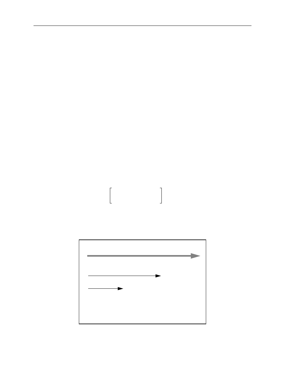
45
It is important to note that the “bootstrapped” zero-coupon curve will have zero-coupon
rates for discrete maturities. The intermediate zero-coupon rates are typically determined by
linear interpolation between the discrete maturities.
C.
Extracting “implied” forward rates from zero-coupon rates
A forward rate is the rate of interest from one period in the future to another period in the
future. It is, for example, the rate one would pay (earn) to borrow (lend) money in one year with a
maturity in two years. Forward interest rates (like zero-coupon rates) are typically not directly
observable and, as a result, they must be derived from the zero-coupon curve; hence the term,
“implied” forward rates.
The implied forward rates are derived from zero-coupon rates from an arbitrage argument.
Specifically, forward borrowing or lending transactions can be replicated with the appropriate
spot transactions. A forward contract, from time
τ
to T, can be replicated at no cost by borrowing
from time t to T and lending the proceeds from t to
τ
(with t <
τ
< T). The result is a cash receipt at
time
τ
and an obligation to pay at time T, with the implied rate between period
τ
and T equal to the
forward rate. The following general expression summarizes this argument algebraically:
.
(A:EQ 11)
The following box provides a 2-period numerical example of the calculation of implied
forward rates:
F t
τ
T
, ,
(
)
1
Z t T
,
(
)
+
(
)
T
t
–
(
)
365
⁄
1
Z t
τ
,
(
)
+
(
) τ
t
–
(
)
365
⁄
-------------------------------------------------------------
365
T
τ
–
------------
1
–
=
time = 0
time = 1
time = 2
Borrow $100 until
Pay $112.36
$100 x (1.06)
2
Invest $100 until
Receive $105
$100 x (1.05)
1
The implied forward rate is 7.01%
You have borrowed $105 and will repay $112.36
($112.36- $105) / $105 = 0.0701.
time = 2 at 6%
time = 1 at 5%
Z(1) = 5%
Z(2) = 6%
Diagram 2: Calculation of “implied” forward rates

46
D.
Mechanics of the estimation
The estimation of Nelson-Siegel or the Svensson model parameters is briefly described in
Figure 2 on page 10 of the text. This appendix provides additional detail on the separate compo-
nents of the estimation, which can be conceptually divided into three parts: the basic mechanical
steps required to generate theoretical bond prices (points C and D of Figure 2); the alternative
specifications of the objective function (point F of Figure 2); and finally, the specifics respecting
the optimization algorithms (represented in point F of Figure 2). The mechanics of the con-
struction of theoretical bond prices and the alternative formulations of the objective function are
described in this section while the optimization strategies are outlined in Section E.
D.1
Construction of theoretical bond prices
The price of a bond is equal to the sum of the discounted values of its cash flows (coupon
payments and principal). Therefore, to generate the vector of theoretical bond prices for selected
Canadian bonds and bills, a matrix of coupon and principal payments of bonds (matrix of bond
cash flows) is built and a matrix of the corresponding coupon and principal payment dates (date
matrix) is also constructed. Using the date matrix and the Nelson-Siegel or the Svensson theo-
retical discount function, a matrix of discount factors (discount matrix) is created relating to the
specific interest and coupon payment dates. The Nelson-Siegel and the Svensson discount
matrices differ only in the functional form of the forward rate curve functions used for the dis-
count function applied.
The discount matrix and the matrix of bond cash flows are then multiplied in an element-
by-element fashion to obtain a matrix of discounted coupon and principal payments (discounted
payment matrix). As a final step, the Nelson-Siegel or the Svensson vector of theoretical bond
prices is obtained by summing all the discounted payments corresponding to each bond in the dis-
counted payment matrix. This process is outlined in the following diagram. For any set of
Svensson parameters, the resulting vector of theoretical bond prices can be calculated.
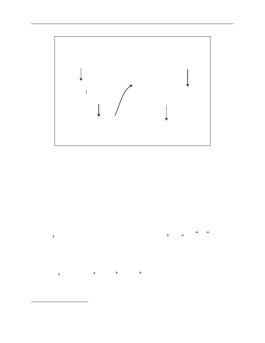
47
D.2
Log-likelihood objective function
This name for the objective function is somewhat of a misnomer because maximum like-
lihood estimation is not actually used. An objective function inspired by a log-likelihood function
is derived but there is no particular concern with the distribution of the error terms. What is sought
instead is a method that incorporates the information in the bid-offer spread—in particular, the
generation of an additional penalty for errors (measured from the mid-price) that fall outside the
bid-offer spread.
The vector of bond prices is a function of X, described as the matrix of inputs (which
includes the cash flow amount and dates), and the vector of term structure parameters. The vector
of errors,
, is defined as the difference between the mid-price (
) and the
estimated price multiplied by a weight matrix (where
is a diagonal matrix with the
weight vector as the elements along the main diagonal) as follows:
12
, where
(A:EQ 12)
12.
is defined as the mid-price,
as the bid-price, and
as the offer-price.
Matrix of bond cash flows:
Date matrix: a matrix of the
Discount matrix: a matrix of
Discounted payment matrix: a matrix
a matrix of all the coupon
and principal payments
specific dates for all coupon
and principal payments
Discount rate function
discount factors relating to each
coupon and principal payment
date
of all the discounted coupon and
principal payments
Vector of theoretical bond prices:
the horizontal sum of each row in
the discounted payment matrix
Diagram 3: Steps in calculating the theoretical price vector
A discount rate is
determined for each
coupon and interest
payment date.
Element-by-element
multiplication of the
payment and discount
matrix produces the discounted
payment matrix.
disc TT M
t
β
o
β
1
β
2
β
3
τ
1
τ
2
,
,
,
,
,
(
)
e
P
M
P
O
P
B
P
O
–
2
-------------------
+
=
diag
ω
( )
P
M
P
B
P
O
e
diag
ω
( )
P
M
f X
β
,
(
)
–
[
]
⋅
=
β
β
0
…β
n
τ
1
…τ
n
,
{
}
=

48
The key assumption of maximum likelihood estimation is the assumption that the errors
are normally distributed with a zero mean and a variance of
. This can be expressed as follows:
.
(A:EQ 13)
Instead, however, of having a specified constant variance for the errors, there is a unique
variance for each observation as one-half of the bid-offer spread or
. This,
therefore, transforms the likelihood function into the following:
13
,
where
(A:EQ 14)
The final step is to derive the log-likelihood function and apply the appropriate weights.
Therefore, in the optimization algorithms, it is desired to maximize the following objective
function:
.
(A:EQ 15)
D.3
Sum of squared errors with penalty parameter objective function
The second objective function used in the estimation of the model is somewhat more
straightforward as it represents a special case of simple sum of squared errors objective function.
Again, the goal is to penalize to a greater extent those errors that fall outside of the bid-offer
spread while maintaining a continuous objective function.
Recall from the previous section (see equation 12) that the vector of bond prices is a
function of a matrix of inputs and a vector of parameters. In the simple case, the error is defined in
the same way as in the previous section, that is:
(A:EQ 16)
The transformation is to multiply the price error by two and divide it by the bid-offer
spread (
) and raise this quotient to the power of
, which can be considered as a
13. Note that
in the likelihood function is set to one. As a result, the likelihood function will differ by a constant
from a more general presentation.
σ
2
e
N 0
σ
2
I
,
(
)
∼
σ
bo
1
2
--- P
B
P
O
–
(
)
=
σ
2
l
β σ
2
Price X
,
,
(
)
2
π
( )
N
2
----
–
Ω
1
2
---
–
e
e
T
Ω
1
–
e
(
)
2
----------------------
–
=
Ω
diag
σ
bo
(
)
[
]
2
=
L
β σ
2
Price X
,
,
(
)
N
2
----
2
π
( )
1
2
---
Ω
ln
–
e
T
Ω
1
–
e
2
------------------
–
ln
–
=
e
P
M
f X
β
,
(
)
–
[
]
=
S
P
B
P
O
–
=
λ

49
penalty parameter (where
and
are diagonal matrices with
and
as the ele-
ments along the main diagonals respectively). This expression is defined as follows:
,
where
.
(A:EQ 17)
It can be seen that, if the error term in the numerator and the bid-offer spread in the
denominator are the same, the value will be one and the exponent will not change its value. The
scaling of the error term in the numerator by a factor of two is intended to make this possible. If
the error term is less than the bid-offer spread, the value of the expression will be less than one
and the exponent will reduce its value, which will correspondingly have less impact in the esti-
mation. Finally, should the error term exceed the bid-offer spread, then the exponent will increase
the size of the expression and increase its influence on the estimation. It is worth noting that, in
this paper’s estimations, the penalty parameter
was maintained at a fairly arbitrary value of two.
It would be possible to increase the penalty for falling outside the bid-offer spread by increasing
the size of the penalty parameter. Thus, the sum of squared errors with a penalty parameter
objective function is formally expressed as follows:
.
(A:EQ 18)
E.
Optimization algorithms
To minimize the weighted sum of the absolute value of price errors, a constrained non-
linear optimization procedure is used. The constraints enhance the speed of the algorithm and
avoid “strange” local optima, which are not economically feasible in the Canadian yield curve
environment.
14
The specific constraints imposed on the parameter values for both models are as
follows:
15
•
Parameters:
,
,
,
,
•
Relative values:
This is both a discussion and a demonstration of the challenges of determining the parameter
values for the parameter models. The two alternative global optimization algorithms that were
designed to deal with this problem are discussed in the following sections.
14. These constraints are practically derived and thus do not come from any economic theory. For example, the
τ
s are
constrained to the range of Government of Canada bond maturities while the
β
s are restricted to values that
provide reasonable shapes for the resulting zero-coupon and forward curves.
15. The constraints on coefficients
β
3
and
τ
2
, however, only apply to the Svensson model.
diag e
( )
diag S
( )
e
S
ψ
( )
λ
ψ
2diag e
( )
diag S
( )
1
–
⋅
=
λ
g
β
Price X
,
(
)
ω
T
Ψ
( )
λ
ω
=
0
β
0
25
<
<
20
–
β
1
20
<
<
25
–
β
2
25
<
<
25
–
β
3
25
<
<
1
12
------
τ
1
30
<
<
1
12
------
τ
2
30
<
<
0
β
0
β
1
+
<

50
E.1
Full-estimation algorithm
This global search algorithm begins with the construction of a matrix of starting
parameter values (
), runs a local search for each parameter set (
),
and
then selects the best solution. Conceptually, what is sought is to partition the parameter space and
run a local search in each subregion. The dimensionality of the problem, however, makes this
practically impossible or, rather, prohibitively time consuming. Therefore, there is an attempt to
simplify the grid by making some assumptions about the possible starting values for the
β
0
and
β
1
parameters. In both the Nelson-Siegel and Svensson models, the
β
0
and
β
1
parameters are not
varied but instead set to “educated guesses” for their values.
16
It is important to note, however,
that for each set of starting parameters, the entire parameter set is estimated. The
β
0
starting value,
which is the asymptote of the instantaneous forward rate function, is set to the YTM of the bond
with the longest term to maturity in the data sample (i.e., the most recently issued 30-year bond).
It is also noted that, given that the sum of
β
0
and
β
1
is the vertical intercept of the instantaneous
forward rate function, the starting value of
β
1
is set to the difference between the longest and
shortest YTM in the data set (i.e., the most recently issued 30-year bond YTM less 30-day
treasury bill rate).
Thus, the previously described values for
β
0
and
β
1
and combinations of different values
for the remaining parameters are used to construct the matrix of starting values. In the Nelson-
Siegel model, nine combinations of the remaining two parameters (
β
2
and
τ
1
) are used in the grid
for a total of 81 (
) sets of starting parameters. In the Svensson model, four combinations of four
parameters (
β
2
, β
3
, τ
1
, τ
2
) are used for a total of 256 (
) different sets of starting values. The grid
used to estimate the Nelson-Siegel model is much finer than that used for the Svensson model.
This is shown by the more robust nature of the results for the Nelson-Siegel model in the text of
the paper. The selection of the number of different combinations of starting values appears to be
arbitrary although it is really a function of the time constraint. Note that five combinations of the
varied parameter set (
β
2
, β
3
, τ
1
, τ
2
) instead of four combinations for the Svensson model amount
to 1,296 (
) different sets of starting values. This would require approximately five times longer
to estimate than the more-than-three hours already required.
Two alternative local search algorithms are used to solve for each row in the matrix of
starting values: sequential quadratic programming (SQP) and the Nelder and Mead Simplex
method. Sequential quadratic programming uses local gradient information to determine the
16. Ricart and Sicsic (1995) use these as constraints in their estimation. The ideas are used in this paper without
constraining the parameters.
S
i j
,
β
β
0
…β
n
τ
1
…τ
n
,
{
}
=
9
2
4
4
6
4
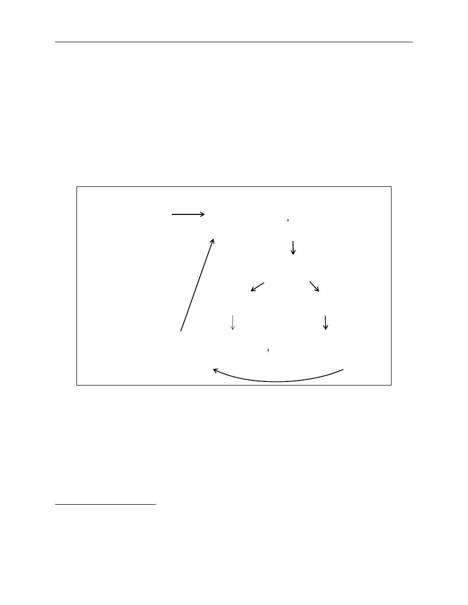
51
direction of movement of the algorithm over the objective function; the Simplex method uses a
series of direct function evaluations to determine the direction of descent.
17
The reason for two
alternative approaches is the difficulties in the estimation of the full model. On occasion, the SQP
algorithm fails to converge. To solve this problem, it was decided to limit the time permitted for
each SQP local search. On failure to converge before a specified period of time (two minutes), it
would be replaced with the more reliable although less accurate Simplex algorithm with which
there had been no convergence problems.
18
Figure 1 provides a simple flow chart of the steps in
the full-estimation algorithm for the Svensson model (the logic of the Nelson-Siegel model is
identical).
Figure 1. A flow chart of the “Svensson model” full-estimation algorithm
E.2
Partial-estimation algorithm
This global search algorithm divides the parameters into two groups, the
β
s (or linear
parameters) and the
τ
s (or the non-linear parameters). It works in a number of steps where one
group of parameters is fixed while the other is estimated. The advantages of estimating one subset
of the parameters while holding the other constant are improved speed of convergence and
increased stability. Indeed, unlike the full-estimation algorithm discussed in the previous section,
17. See C. F. Garvin, “Introduction to Algorithms,” in Financial Toolbox: For Use with MATLAB (Natick, Mass.:
MathWorks, 1996) for a good discussion of the SQP algorithm, and Nelder and Mead (1965) for the original
description of the surprisingly straightforward Simplex algorithm.
18. Two minutes was chosen as the cut-off for the SQP algorithm through a process of trial and error.
Matrix,
S, of 256
different sets of
starting values
(
).
S
256 6
,
Select row
i of the matrix
and run the SQP local
search algorithm (
).
S
i 6
,
Does it converge
within 2 minutes?
YES
NO
Run the Simplex
local search
algorithm.
Save results and run the next row
of the starting value matrix (
).
S
i
1 6
,
+
From the 256 different
sets of starting values, the
best solution is selected.

52
each step of the partial-estimation algorithm was estimated using the SQP algorithm exclusively
and no convergence problems were encountered.
Whenever certain sets of parameters are fixed, there is a concern that the solution is being
constrained from its optimum. The partial estimations were performed in two separate streams in
an attempt to mitigate this concern. The first stream fixes the
τ
parameters while estimating the
β
s,
and then proceeds to fix the
β
s and estimate the
τ
s. The second stream proceeds in reverse
fashion: It fixes the
β
s and estimates the
τ
s, and subsequently fixes the
τ
s and estimates the
β
s.
Each step of both streams uses the best solution or, rather, set of estimated parameters from the
previous step. Specifically, a new matrix of starting parameters is then built around these esti-
mated parameters to perform a new round of partial estimations. Note that, in each new matrix of
starting parameters, only those parameters that are fixed in that round of estimation are varied,
while the estimated parameters use the previous step’s estimated parameters as starting values.
Upon completion of both streams, all the estimations performed (both partial and full) are sorted
by the value of their objective function and the best solution is selected. The two main streams
(termed Step 1 and Step 2) are outlined in Figure 2.
Note that both estimation streams begin with a relatively coarse matrix of starting param-
eters; that is, using a wide range of values for both the fixed and the estimated parameters. This
allows, in subsequent steps, the estimation of the parameters that were fixed in the first step using
a narrower grid. It thereby permits the analysis to be focused around the best estimated values
obtained in the first step. The estimation of all the parameters can therefore be performed in the
final step for a small number of starting parameters.

53
Figure 2. A flow chart of “Svensson model” partial-estimation algorithm
• Construct matrix of starting
values,
. Vary the
τ
s
for a total
of 81 rows (
).
S
β
˜
τ
,
9
2
• Estimate, using each row of this
starting-value matrix.
• Select the 4 best solutions of all
the estimations (from either step)
and estimate the full model.
τ
s
fixed and
β
s estimated
• Select 3 best solutions.
Construct starting-value matrices
around each solution (25 rows in
each).
• Estimate, using each row of
these starting-value matrices.
STEP 1.0
• Construct a new matrix of
starting values,
. Vary the
β
s
for a total of 81 rows (
).
S
β τ
˜
,
3
4
• Estimate, using each row of this
starting-value matrix.
• Select the 2 best solutions.
Construct starting-value matrices
around each solution (25 rows in
each).
• Estimate, using each row of
these starting-value matrices.
STEP 1.1
• Construct matrix of starting
values,
. Vary
β
1
,
β
2
, and
β
3
for a total of 147 rows (
).
S
β τ
˜
,
3
1
2
7
⋅
• Estimate, using each row of
starting-value matrix.
• Select the 4 best solutions of all
the estimations (from either step)
and estimate the full model.
• Select 2 best solutions.
Construct starting-value matrices
around each solution (81 rows in
each).
• Estimate, using each row of
these starting-value matrices.
STEP 2.0
• Construct a new matrix of
starting values,
. Vary the
β
s
for a total of 81 rows (
).
S
β τ
˜
,
3
4
• Estimate, using each row of this
starting-value matrix.
• Select 2 best solutions.
Construct starting-value matrices
around each solution (81 rows in
each).
• Estimate, using each row of
these starting value matrices.
STEP 2.1
STEP 1.2
STEP 2.2
Select the best solution from among all the
estimations in steps 1 and 2.
STEP 1
τ
s
estimated and
β
s fixed.
STEP 2


55
REFERENCES
Atta-Mensah, J. 1997. “Extracting Information from Financial Instruments and the Implication for Monetary Policy:
A Survey.” Department of Monetary and Financial Analysis, Bank of Canada. Photocopy.
Barker, W. 1996. “Bond Pricing: The ‘Street’ vs. Bank of Canada Formulae.” Securities Department, Bank of
Canada. Photocopy.
Bekdache, B. and C.F. Baum. 1994. “Comparing Alternative Models of the Term Structure of Interest Rates.” Boston
College, Department of Economics, Working Paper 271.
Bliss, R.R. 1991. “Testing Term Structure Estimation Methods.” PhD thesis. Graduate School of Business, University
of Chicago.
———. 1996. “Testing Term Structure Estimation Methods.” Federal Reserve Bank of Atlanta Working Paper
96-12a.
Boisvert, S. and N. Harvey. 1998. “The declining supply of treasury bills and the Canadian money market.” Bank of
Canada Review (Summer): 53–69.
Bolder, D. and S. Boisvert. 1998. “Easing Restrictions on the Stripping and Reconstitution of Government of Canada
Bonds.” Bank of Canada Working Paper 98-8.
Branion, A. 1995. “The Government of Canada bond market since 1980.” Bank of Canada Review (Autumn): 3–20.
Caks, J. 1977. “The Coupon Effect on Yield to Maturity.” Journal of Finance 32: 103–115.
Côté, A., J. Jacob, J. Nelmes, and M. Whittingham. 1996. “Inflation expectations and Real Return Bonds.” Bank of
Canada Review (Summer): 41–53.
Das, S. 1993a. “Duration and Swap Hedging Technology.” Appendix B of Chapter 33,“Swap Portfolio Risk
Management Techniques: Portfolio Hedging Techniques.” In Swap & Derivative Financing, rev. ed.,
1055-1060. Chicago: Probus.
———. 1993b. “Calculating Zero Coupon Rates.” Appendix of Chapter 8, “Swap Yield Mathematics and Swap
Valuation.” In Swap & Derivative Financing, rev. ed., 219–225. Chicago: Probus.
Fabozzi, F.J. and T.D. Fabozzi, eds. c1995. The Handbook of Fixed Income Securities. 4th ed. Burr Ridge, Ill.: Irwin.
Fettig, K. 1994. “The Government of Canada treasury bill market and its role in monetary policy.” Bank of Canada
Review (Spring): 35–53.
Fettig, K. and G. Lee. 1992. “The Par and Topical Yield Curves: Why do they Differ?” File 385-5-3. Securities
Department, Operations Analysis, Bank of Canada. Photocopy.
Garvin, C.F. 1996. Financial Toolbox. For Use with MATLAB. Natick, Mass.: MathWorks.
Kamara, A. 1990. “Liquidity and Short-Term Treasury Yields.” Graduate School of Business Administration
Working Paper, University of Washington.
Kiff, J. 1996. “Price and Yield Calculations on Government of Canada Domestic Securities.” Financial Markets
Department, Bank of Canada. Photocopy.
Litzenberger, R.H. and J. Rolfo. 1984. “An International Study of Tax Effects on Government Bonds.” Journal of
Finance 39: 1–22.

56
McCulloch, J. 1971. “Measuring the Term Structure of Interest Rates.” Journal of Business 44: 19–31.
Nelder, J.A. and R. Mead. 1965. “Simplex Method for Function Minimization.” Computer Journal 7: 308–313.
Nelson, C.R. and A.F. Siegel. 1987. “Parsimonious Modeling of Yield Curves.” Journal of Business 60: 473–489.
Ricart, R. and P. Sicsic. 1995. “Estimating the Term Structure of Interest Rates from French Data.” Banque de France
Bulletin Digest (22): 473–489.
Schich, S. 1996. “Alternative specifications of the German term structure and its information content regarding
inflation.” Economic Research Group of the Deutsche Bundesbank, Discussion paper 8/96. October.
Shea, G.S. 1984. “Pitfalls in Smoothing Interest Rate Term Structure Data: Equilibrium Models and Spline
Approximations.” Journal of Financial and Quantitative Analysis 19: 253–269.
Suits, D.B., A. Mason, and L. Chan. 1977. “Spline Functions Fitted by Standard Regression Methods.” Review of
Economics and Statistics 6: 132–139.
Svensson, L.E. 1994. “Estimating and Interpreting Forward Interest Rates: Sweden 1992-1994.” Centre for Economic
Policy Research, Discussion Paper 1051.
Svensson, L.E. and P. Söderlin. 1997. “New Techniques to Extract Market Expectations from Financial Instruments.”
Centre for Economic Policy Research, Discussion Paper 1556.
Vasicek, O.A. and H.G. Fong. 1982. “Term Structure Modeling Using Exponential Splines.” Journal of Finance
37: 339–348.

Bank of Canada Technical Reports
Rapports techniques de la Banque du Canada
Technical reports are generally published in the language of the author, with an abstract in both official languages.
Les rapports techniques sont publiés généralement dans la langue utilisée par les auteurs; ils sont cependant
précédés d’un résumé bilingue.
1999
84
Yield Curve Modelling at the Bank of Canada
D. Bolder and D. Stréliski
1998
83
The Benefits of Low Inflation: Taking Stock
B. O’Reilly
82
The Financial Services Sector: Past Changes and Future Prospects
C. Freedman and C. Goodlet
81
The Canadian Banking System
C. Freedman
1997
80
Constraints on the Conduct of Canadian Monetary Policy in the 1990s:
Dealing with Uncertainty in Financial Markets
K. Clinton and M. Zelmer
79
Measurement of the Output Gap: A Discussion of Recent Research at
the Bank of Canada
P. St-Amant and S. van Norden
1996
78
Do Mechanical Filters Provide a Good Approximation of Business Cycles?
A. Guay and P. St-Amant
77
A Semi-Structural Method to Estimate Potential Output:
Combining Economic Theory with a Time-Series Filter
The Bank of Canada’s New Quarterly Projection Model, Part 4
L. Butler
76
Excess Volatility and Speculative Bubbles in the Canadian Dollar:
J. Murray, S. van Norden,
Real or Imagined?
and R. Vigfusson
75
The Dynamic Model: QPM, The Bank of Canada’s
D. Coletti, B. Hunt,
New Quarterly Projection Model, Part 3
D. Rose, and R. Tetlow
74
The Electronic Purse: An Overview of Recent Developments and Policy Issues
G. Stuber
1995
73
A Robust Method for Simulating Forward-Looking Models,
J. Armstrong, R. Black,
The Bank of Canada’s New Quarterly Projection Model, Part 2
D. Laxton, and D. Rose
1994
72
The Steady-State Model: SSQPM, The Bank of Canada’s New
R. Black, D. Laxton,
Quarterly Projection Model, Part 1
D. Rose, and R. Tetlow
71
Wealth, Disposable Income and Consumption: Some Evidence for Canada
R. T. Macklem
70
The Implications of the FTA and NAFTA for Canada and Mexico
W. R. White
Copies of the above titles and a complete list of Bank of Canada technical reports are available from:
Pour obtenir des exemplaires des rapports susmentionnés et une liste complète des rapports techniques de la Banque
du Canada, prière de s’adresser à :
PUBLICATIONS DISTRIBUTION
DIFFUSION DES PUBLICATIONS
Bank of Canada, Ottawa, Ontario, Canada K1A 0G9
Banque du Canada, Ottawa (Ontario) K1A 0G9
Tel: (613) 782-8248; fax: (613) 782-8874
Tél : (613) 782-8248; télécopieur : (613) 782-8874
Document Outline
- Technical Report No. 84 / Rapport technique no 84
- Yield Curve Modelling at the Bank of Canada
- February 1999
- ABSTRACT
- RÉSUMÉ
- 1. INTRODUCTION
- 2. THE MODELS
- 2.1 The Super-Bell model
- 2.2 The Nelson-Siegel and Svensson models
- (EQ 6)
- (EQ 7)
- (EQ 8)
- (EQ 9)
- (EQ 10)
- (EQ 11)
- (EQ 12)
- Figure 1. A decomposition of the forward term structure functional form
- Figure 2. Steps in the estimation of Nelson-Siegel and Svensson models
- Figure 3. Estimation of Nelson-Siegel forward curves for 17 January 1994 (81 different sets of st...
- Figure 4. Estimation of Svensson forward curves for 17 January 1994 (256 different sets of starti...
- 3. DATA
- 4. EMPIRICAL RESULTS
- 15 February 1993
- 15 August 1988
- 15 January 1990
- 15 July 1993
- 18 August 1988
- 15 May 1990
- 17 January 1994
- 23 August 1988
- 15 August 1990
- 16 May 1994
- 29 August 1988
- 13 December 1990
- 15 August 1994
- 15 February 1991
- 14 April 1989
- 15 February 1995
- 25 February 1991
- 15 June 1989
- 17 July 1995
- 4 March 1991
- 15 August 1989
- 15 February 1996
- 11 March 1991
- 16 October 1989
- 15 August 1996
- 15 June 1998
- 15 December 1989
- 16 December 1996
- 15 July 1998
- 15 March 1990
- Minimum amount outstanding
- Can$500 million
- Divergence from par: | Coupon - YTM |
- 500 basis points
- Inclusion of treasury bills
- Yes
- Inclusion of bonds with less than 2 years TTM
- No
- Normal
- 100,707.6
- 100,707.6
- 86,799.7
- 87,755.1
- 51,813.5
- 51,813.5
- 23,997.7
- 25,908.4
- n/a
- Flat
- 61,707.3
- 61,707.3
- 54,616.2
- 54,837.2
- 97,587.4
- 97,743.8
- 83,405.1
- 83,643.4
- n/a
- Inverted
- 24,006.0
- 24,006.0
- 21,016.5
- 21,432.2
- 40,660.5
- 40,660.5
- 34,681.5
- 35,182.6
- n/a
- Total
- 62,140.3
- 62,140.3
- 54,144.1
- 54,674.8
- 63,353.8
- 63,406.0
- 47,361.5
- 48,244.8
- n/a
- Normal
- 58.8%
- 10.0%
- 17.1%
- 6.1%
- 58.6%
- 5.7%
- 16.8%
- 1.8%
- n/a
- Flat
- 53.1%
- 17.3%
- 35.8%
- 5.4%
- 52.5%
- 1.3%
- 35.1%
- 8.9%
- n/a
- Inverted
- 76.8%
- 23.0%
- 35.1%
- 9.8%
- 76.3%
- 34.0%
- 32.9%
- 2.4%
- n/a
- Total
- 62.8%
- 16.8%
- 29.3%
- 7.1%
- 62.5%
- 17.5%
- 28.2%
- 4.4%
- n/a
- Normal
- 8.6
- 8.6
- 6.5
- 6.5
- 8.8
- 8.6
- 6.5
- 6.5
- 11.3
- Flat
- 25.5
- 25.5
- 24.4
- 25.0
- 25.5
- 25.5
- 24.4
- 24.9
- 25.7
- Inverted
- 18.1
- 18.1
- 18.5
- 18.5
- 18.1
- 18.1
- 18.5
- 18.5
- 26.2
- Total
- 17.4
- 17.4
- 16.5
- 16.7
- 17.4
- 17.4
- 16.5
- 16.6
- 21.1
- Normal
- 6.6
- 6.6
- 5.1
- 5.0
- 6.6
- 6.6
- 5.1
- 5.0
- 9.5
- Flat
- 17.4
- 17.4
- 16.4
- 16.8
- 17.4
- 17.5
- 16.4
- 16.7
- 17.0
- Inverted
- 13.4
- 13.5
- 13.1
- 13.1
- 13.4
- 13.4
- 13.1
- 13.1
- 18.4
- Total
- 12.5
- 12.5
- 11.5
- 11.6
- 12.5
- 12.5
- 11.5
- 11.6
- 15.0
- Normal
- 9.7%
- 9.7%
- 11.5%
- 11.5%
- 9.7%
- 9.7%
- 11.4%
- 11.5%
- 6.9%
- Flat
- 4.3%
- 4.3%
- 3.4%
- 3.2%
- 4.3%
- 4.2%
- 3.7%
- 3.5%
- 3.8%
- Inverted
- 5.0%
- 5.0%
- 3.8%
- 4.1%
- 5.0%
- 5.0%
- 4.0%
- 4.2%
- 2.1%
- Total
- 6.3%
- 6.3%
- 6.3%
- 6.3%
- 6.3%
- 6.3%
- 6.3%
- 6.4%
- 4.3%
- Normal
- 47.0%
- 47.0%
- 50.0%
- 48.4%
- 47.0%
- 47.0%
- 50.2%
- 48.7%
- 55.8%
- Flat
- 47.5%
- 47.5%
- 46.5%
- 46.9%
- 47.5%
- 47.9%
- 46.6%
- 47.0%
- 52.5%
- Inverted
- 56.3%
- 56.3%
- 53.2%
- 53.5%
- 56.3%
- 56.3%
- 53.2%
- 53.7%
- 60.8%
- Total
- 50.3%
- 50.3%
- 50.0%
- 49.6%
- 50.3%
- 50.4%
- 50.0%
- 49.8%
- 56.4%
- Normal
- 53.0%
- 53.0%
- 50.0%
- 51.6%
- 53.0%
- 53.0%
- 49.8%
- 51.3%
- 44.2%
- Flat
- 52.5%
- 52.5%
- 53.5%
- 53.1%
- 52.5%
- 52.1%
- 53.4%
- 53.0%
- 47.5%
- Inverted
- 43.7%
- 43.7%
- 46.8%
- 46.5%
- 43.7%
- 43.7%
- 46.8%
- 46.3%
- 39.2%
- Total
- 49.7%
- 49.7%
- 50.0%
- 50.4%
- 49.7%
- 49.6%
- 50.0%
- 50.2%
- 43.6%
- Normal
- 11.3
- 1.7
- 47.5
- 4.1
- 11.5
- 1.6
- 48.5
- 4.4
- 0.5
- Flat
- 10.7
- 2.0
- 49.0
- 4.6
- 11.1
- 2.2
- 50.3
- 6.2
- 0.5
- Inverted
- 13.9
- 2.1
- 46.3
- 4.5
- 14.2
- 2.2
- 47.3
- 4.6
- 0.5
- Total
- 12.0
- 1.9
- 47.6
- 4.4
- 12.3
- 2.0
- 48.7
- 5.1
- 0.5
- Normal
- 0.25
- 0.17
- 3.20
- 0.44
- 0.26
- 0.18
- 3.27
- 0.60
- 0.00013
- Flat
- 0.24
- 0.37
- 3.31
- 0.54
- 0.25
- 0.30
- 3.40
- 0.88
- 0.00013
- Inverted
- 0.31
- 0.47
- 3.13
- 0.66
- 0.32
- 0.43
- 3.20
- 0.71
- 0.00013
- Total
- 0.27
- 0.33
- 3.21
- 0.55
- 0.28
- 0.30
- 3.29
- 0.73
- 0.00013
- Normal
- 52.3
- 61.2
- 56.2
- 26.2
- Flat
- 74.5
- 94.2
- 89.2
- 56.5
- Inverted
- 83.3
- 101.7
- 97.2
- 65.5
- Total
- 70.0
- 85.7
- 80.9
- 49.4
- Minimum amount outstanding
- Can$2,500 million
- Can$500 million
- Divergence from par: | Coupon - YTM |
- 250 basis points
- 500 basis points
- Inclusion of treasury bills
- Yes
- Yes
- Inclusion of bonds with less than 2 years TTM
- No
- No
- Normal
- 6.5
- 6.9
- 5.0
- 5.4
- 11.5%
- 11.9%
- Flat
- 25.0
- 19.6
- 16.8
- 13.7
- 3.2%
- 3.1%
- Inverted
- 18.5
- 15.8
- 13.1
- 11.7
- 4.1%
- 5.4%
- Total
- 16.7
- 14.1
- 11.6
- 10.2
- 6.3%
- 6.8%
- Normal
- 4.1
- 4.1
- 0.44
- 0.44
- Flat
- 4.6
- 4.8
- 0.55
- 0.67
- Inverted
- 4.5
- 4.5
- 0.66
- 0.60
- Total
- 4.4
- 4.5
- 0.55
- 0.57
- Normal
- 87,755.1
- 87,732.9
- 21.6%
- 20.2%
- Flat
- 54,837.2
- 49,560.0
- 18.2%
- 17.9%
- Inverted
- 21,432.2
- 20,352.3
- 31.3%
- 31.9%
- Total
- 54,674.8
- 52,548.4
- 23.7%
- 23.3%
- Minimum amount outstanding
- Can$500 million
- Can$500 million
- Can$500 million
- Divergence from par: | Coupon - YTM |
- 500 basis points
- 500 basis points
- 500 basis points
- Inclusion of treasury bills
- No
- Yes
- Yes
- Inclusion of bonds with less than 2 years TTM
- Yes
- Yes
- No
- Normal
- 6.5
- 6.8
- 6.4
- 5.0
- 5.3
- 4.8
- 11.5%
- 14.4%
- 14.0%
- Flat
- 25.0
- 28.5
- 27.3
- 16.8
- 15.8
- 15.2
- 3.2%
- 7.8%
- 5.9%
- Inverted
- 18.5
- 19.8
- 17.2
- 13.1
- 13.9
- 13.0
- 4.1%
- 6.0%
- 5.0%
- Total
- 16.7
- 18.4
- 17.0
- 11.6
- 11.7
- 11.0
- 6.3%
- 9.4%
- 8.3%
- Normal
- 4.1
- 5.2
- 4.4
- 0.44
- 1.23
- 0.95
- Flat
- 4.6
- 4.9
- 4.9
- 0.55
- 1.08
- 1.09
- Inverted
- 4.5
- 5.0
- 5.2
- 0.66
- 1.17
- 0.96
- Total
- 4.4
- 5.1
- 4.8
- 0.55
- 1.16
- 1.00
- Normal
- 87,755.1
- 75,149.9
- 36,369.9
- 21.6%
- 13.7%
- 10.6%
- Flat
- 54,837.2
- 45,207.7
- 61,362.5
- 18.2%
- 12.7%
- 8.6%
- Inverted
- 21,432.2
- 16,857.1
- 24,700.8
- 31.3%
- 22.9%
- 21.1%
- Total
- 54,674.8
- 45,738.2
- 40,811.1
- 23.7%
- 16.4%
- 13.4%
- TECHNICAL APPENDIXES
- Bank of Canada Technical Reports Rapports techniques de la Banque du Canada
Wyszukiwarka
Podobne podstrony:
Ustawa z dnia 25 06 1999 r o świadcz pien z ubezp społ w razie choroby i macierz
brzuch 1999 2000
chojnicki 1999 20 problemy GP
Porty morskie i żegluga morska w Polsce w latach 1999 2001
ABS Octawia 1999
1999 05 05 0953
ED 1999 1 41
Badanie wahadła skrętnego, Studia, Pracownie, I pracownia, 7 Badanie drgań wahadła skrętnego {torsyj
Okręgi wojskowe od roku 1999, wiedza o siłach zbrojnych
MATHEMATICS HL May 1999 P1
1999 02 str 24 25 Chaotyczne rachunki
1999 12 22 2757
1999 06 Szkoła konstruktorów
0415191246 Routledge Humes Naturalism May 1999
PN EN 60099 5 1999 Ograniczniki przepięć Zasady doboru
897656 1300SRM0568 (10 1999) UK EN
więcej podobnych podstron