A Behavioural Biometric System Based on

Human Computer Interaction

Hugo Gamboa

a

and Ana Fred

b

a

Escola Superior de Tecnologia de Set´

ubal,

Campo do IPS, Estefanilha, 2914-508 Set´

ubal, Portugal;

b

Instituto de Telecomunica¸c˜

oes, Instituto Superior T´

ecnico IST - Torre Norte,

Piso 10, Av. Rovisco Pais 1049-001, Lisboa, Portugal

ABSTRACT

In this paper we describe a new behavioural biometric technique based on human computer interaction. We
developed a system that captures the user interaction via a pointing device, and uses this behavioural information
to verify the identity of an individual. Using statistical pattern recognition techniques, we developed a sequential
classifier that processes user interaction, according to which the user identity is considered genuine if a predefined
accuracy level is achieved, and the user is classified as an impostor otherwise. Two statistical models for the
features were tested, namely Parzen density estimation and a unimodal distribution. The system was tested
with different numbers of users in order to evaluate the scalability of the proposal . Experimental results show
that the normal user interaction with the computer via a pointing device entails behavioural information with
discriminating power, that can be explored for identity authentication.

Keywords:

Biometric authentication, feature extraction, behavioural biometrics, human computer interaction,

statistical learning

1. INTRODUCTION

With the establishment of the information society, personal identification systems have gained an increased
interest, either for security or personalization purposes. Traditionally, computer systems have based identification
procedures on something that one has (keys, magnetic cards or chip cards) or something that one knows (personal
identification numbers and passwords). These systems can easily fail to serve their objective in situations of loss
or lent of a key or card, or in cases of forgotten passwords or disclosure of codes. Biometric authentication or
identification systems use something one is, creating more reliable systems, with higher immunity to authorization
theft, loss or lent.

1.1. Biometrics Technologies

Personal identification or authentication using biometrics applies pattern recognition techniques to measurable
physiological or behavioural characteristics.

1, 2

There are two types of biometric systems that enable the link between a person and his/her identity.

3

Identity

verification (or authentication) occurs when a user claims who he is and the system accepts (or declines) his
claim. Identity identification (sometimes called search) occurs when the system establishes a subject identity (or
fails to do it) without any prior claim.

A Biometric system can be based on any physiological or behavioural characteristics as long as the following

properties are fulfilled

2

: (i) Universality — Every person should have the characteristics. (ii) Uniqueness — No

two persons should be the same in terms of the biometric characteristics. (iii) Permanence — The characteristics
should be invariant with time. (iv) Collectability — The characteristics must be measurable quantitatively and
easy to acquire. (v) Performance — The biometric technique accuracy level. (vi) Acceptability — The level

Further author information: (Send correspondence to H.G.)

H.G.: E-mail: [e-mail], Telephone: [phone]
A.F.: E-mail: [e-mail]

of user acceptance of the biometric system. (vii) Circumvention — The level of difficulty in order to forge an
identification/authentication.

Biometric systems have been applied to a broad range of applications on several fields of our society such

as

4, 5

: forensic science, financial and trade security, physical access control check points, information systems

security, customs and immigration, national identification cards, and driver licences, among other examples.

Listing the biometric techniques currently used, or under research, we found that most of them explore

characteristics extracted from: face, fingerprint, hand geometry, hand vein, iris, retinal pattern, signature, voice-
print, facial thermogram, DNA, palm print, body odor, keystroke dynamics, ear shape, fingernail bed.

A biometric technique is normally accompanied by some metrics that evaluate its performance.

6

Two types

of decisions can be made by a biometric system: classify an individual as genuine or as an impostor. For each
decision an error can be made: a false rejection (type 1 error) — a legitim user is rejected by the system; a
false acceptance (type 2 error) — an impostor is accepted by the system. The number of false rejections / false
acceptances is typically expressed as a percentage of access attempts. The biometric community uses these rates,
called false rejection rate (FRR) and false acceptance rate (FAR), to express the security of a system. The equal
error rate (EER) (defined as the value at which FAR and FRR are equal), and the receiving operating curve
(ROC) (the graphic of FAR as a function of FRR) are additional performance metrics that better express the
identification accuracy of the biometric system.

All these metrics (FAR, FRR, EER and ROC) depend on the collected test data. In order to generalize

the performance numbers to the population of interest, the test data should

7

: (i) be large enough to represent

the population (ii) contain enough samples from each category of the population (from genuine individuals and
impostors).

1.2. Human Behaviour in Biometrics

Biometric techniques can be divided into physiological and behavioural. A physiological trait tends to be a more
stable physical characteristic, such as finger print, hand silhouette, blood vessel pattern in the hand, face or back
of the eye. A behavioural characteristic is a reflection of an individual’s psychology. Because of the variability
over time of most behavioural characteristics, a biometric system needs to be designed to be more dynamic and
accept some degree of variability. On the other hand, behavioural biometrics are associated with less intrusive
systems, conducing to better acceptability by the users.

Handwritten signature

8910

is one of the first accepted civilian and forensic biometric identification technique

in our society. Although there have been some disputes about authorship of handwritten signatures, human
verification is normally very accurate in identifying genuine signatures. The biometric field of computer verifica-
tion of handwritten signatures introduced the signature dynamics information to further reduce the possibility
of fraud.

Another behavioural biometric technique is speaker recognition via his voice print.

11

Despite the occurrences

of some changes to the speakers voice during disease periods, global speech characteristics such as user pitch,
dynamics, and waveform analyzed using speech recognition techniques have been successfully applied in several
systems.

Keystroke dynamics (or typing rhythms)

12

is a innovative behavioural biometric technique. This method

analyzes the way a user types on a terminal, by monitoring the keyboard input. Both the National Science
Foundation and National Institute of Standards and Technology have conducted studies that concluded that
typing patterns are quite unique. The advantages of keystroke dynamics include the low level of detraction
from the regular computer work, because the user would be entering keystrokes when giving a password to the
system. Since the input device is the existing keyboard, the technology has a reduced cost compared to expensive
biometrics acquisition devices.

We have found two different technique related with the user behaviour, that can’t be considered as biometrics

but that have some interesting characteristics related to our work. A user identification system

13

was constructed

based on a piece of text (the system used an entire handwritten page), producing an identification of an individual
based on independent text.

Graphical passwords

14

have been proposed as a more secure system than normal text passwords. The user

sketches a small picture using an electronic pen (the system is proposed to be used in Person Digital Assistants
(PDAs) with graphical input via a stylus). The secret draw is more memorable and present more diversity than
text passwords.

1.3. Our Proposal - User Interaction Behaviour as an Identity Source

In this paper we propose a new behavioural biometric technique based on human computer interaction via
a pointing device, typically a mouse pointer. The normal interaction through this device is analyzed for the
extraction of behavioural information in order to link an identification claim to an individual.

We developed a prototype system,

15

accessed via a web browser, that presents the memory game to the

user: a grid of tiles is presented, each tile having associated a hidden pattern, which is shown for a brief period
of time upon clicking on it; the purpose of the game is to identify the matching tiles (equal patterns). The user
interaction through the web page is recorded and is used for the authentication process.

In the following section we describe the architecture of the developed prototype system. Section 3 presents the

recognition system, focusing on the feature extraction procedures, feature selection, sequential classification and
finally the statistical learning algorithms. Section 4 presents experimental results obtained using the collected
data. Conclusions and future work are presented in section 5.

2. SYSTEM ARCHITECTURE

An experimental system was developed to verify the possibility of discriminating between users using their
computer interaction information, specifically based on mouse movements performed between successive clicks,
which we will call a stroke.

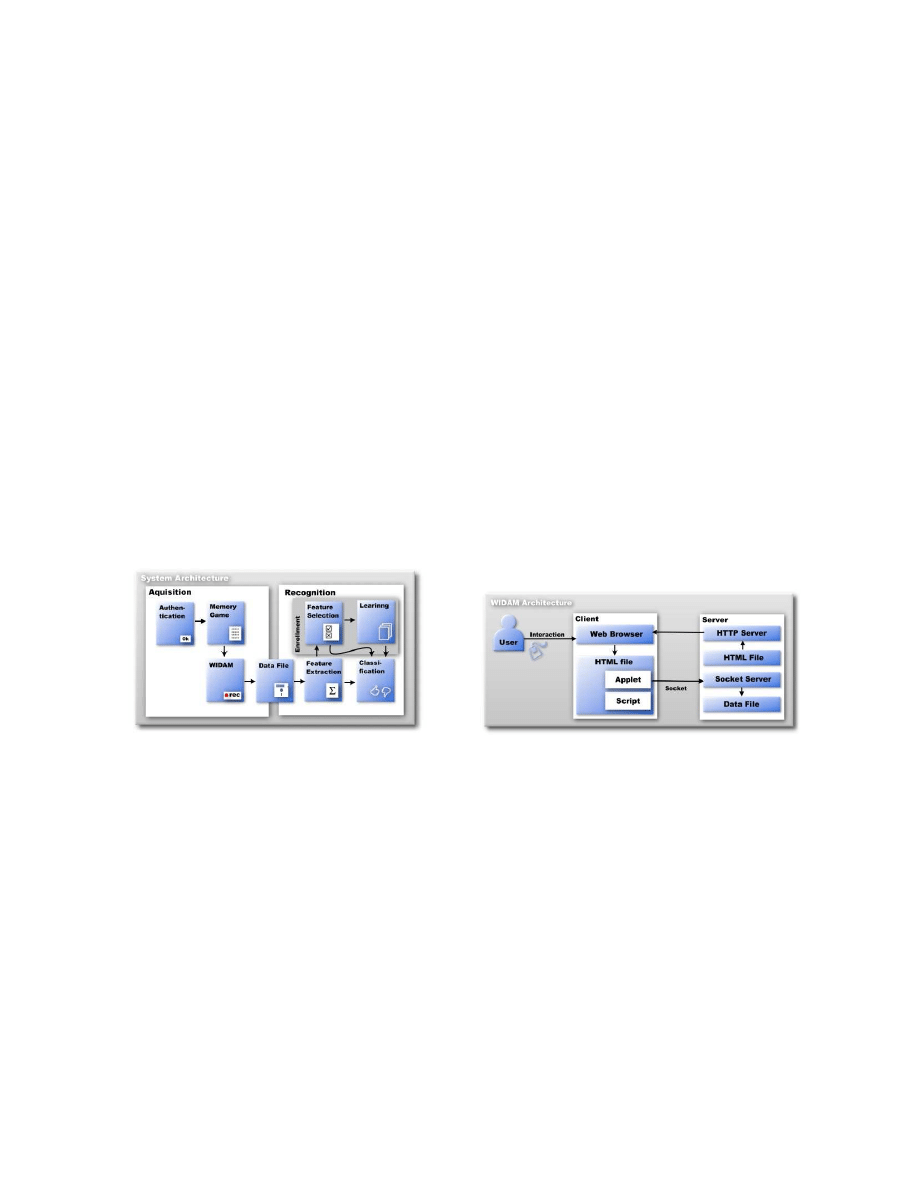
The overall system is divided into two main parts: (i) the acquisition system, that collects user interaction

data and stores it in data files; (ii) the recognition system, that reads from the interaction files, classifies the
user interaction data, giving an estimate of the likelihood of the claimed user being the genuine author of the
interaction. Additionally, the Recognition System has built in procedures for computing indicators about the
achieved performance. Figure 1 presents the two part system and its building blocks.

Figure 1.

The system architecture.

Figure 2.

The WIDAM module architecture.

The acquisition system works over the world wide web, installed in a web server. First, it presents a web

page to the user, asking for his identification (name, and a personal number). Then the system presents an
interaction acquisition page with the memory game (that could be any html web page). This page is monitored
by an application developed for this purpose, that records all the user interaction in a file stored in the web
server.

The recognition system reads the interaction data from the stored data files, and starts a feature extraction

procedure, by applying some mathematical operations (see section 3.1). The classifier (see section 3.3) receives
a sequence of strokes and decides to accept or reject the user as genuine.

The system has an enrolment phase, where the global set of extracted features are used by an algorithm that

selects a set of best features for each user, using the equal error rate as performance measure (feature selection

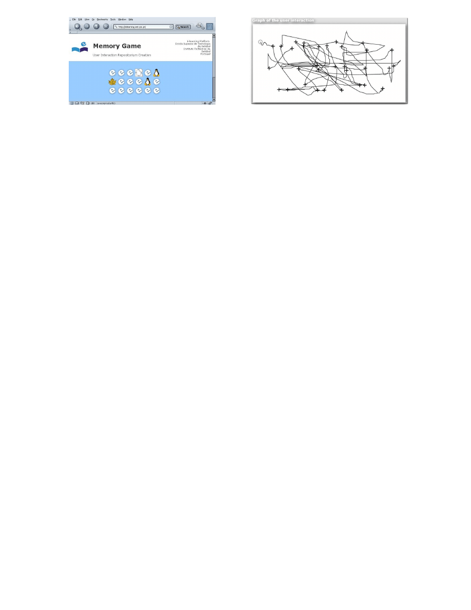
Figure 3.

Interaction test page: the memory game.

Figure 4.

Graph of the user interaction in the memory

game.

block in figure 1). The classifier learning phase consists of the estimation of the probability density functions for
the users data.

2.1. Acquisition System and Data Sets

We needed to collect significant amounts of interaction data associated to their “authors”. The users should
be motivated to spend some time (10-15 minutes), in an interaction environment accessible through the world
wide web. To this purpose, we developed a couple of web pages. One page is used for user identification. The
page presents the objective of the system, stating that the user interaction with the following web pages will be
monitored and recorded in a server machine. The other page is an Interaction Acquisition page, a normal html
page with some extra code embedded to enable interaction monitoring. To motivate the user to spend some
minutes in our page, we decided to use a game, the memory game (see figure 3), in order to be interesting and
time consuming, while the user is actively interacting with the computer. The system does not use the user
performance on the game, but only the interaction characteristics. Scores, playing tactics, playing errors, or
other type of information that could be associated to the author, is ignored. The data that is recorded concerns
only of physical interaction with the web page, namely mouse movements and mouse clicks. Since the type of
data recorded is content independent, this acquisition system can be applied to any web page, associated with
another game, or even to a set of linked web pages.

The recording module is called Web Interaction Display and Monitoring, WIDAM.

16

The WIDAM module

works in a client server architecture as depicted in figure 2. The client is an html page with an embedded java
applet and javascript code that is responsible for opening a communication channel (an internet socket) with the
server, and monitoring user interaction activity events, transmitting these events to the server. Figure 4 depicts
a graph of the interaction collected during an entire memory game.

We asked 50 volunteers (engineering students) to use the system, playing several games during about 10-15

minutes. This way, we created an interaction repository of approximately 10 hours of interaction.

3. RECOGNITION SYSTEM

3.1. Feature Extraction

The input of the recognition system is the interaction data from the users, recorded using the WIDAM module
described previously. ¿From the several events captured only the mouse move and mouse click events are used.
For feature extraction we explore the following raw data: the pointing device absolute position, x- and y-
coordinates; the event type (mouse moves and mouse clicks); and the time when these events occur.

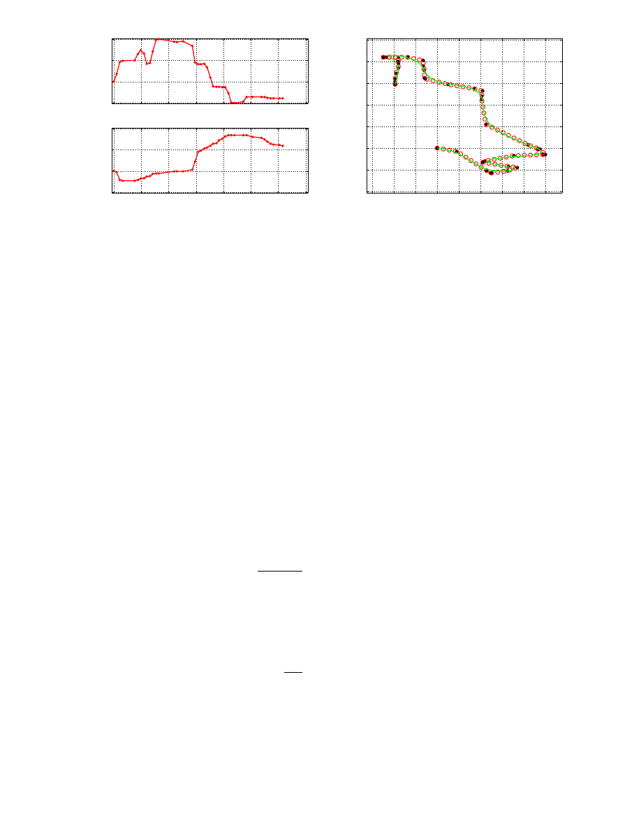
We define stroke as the set of points between two mouse clicks. Figure 5 shows an example of a stroke,

plotting the evolution of the x-y coordinates of the mouse (input vectors) over time. Figure 6 presents the
corresponding x-y representation. The recognition system uses three input vectors of length n to represent a
stoke, with n being the number of mouse move events generated in this pattern:

• x

i

, i = 1...n — the horizontal coordinate of the mouse, sampled at time t

i

.

0

0.5

1

1.5

2

2.5

3

3.5

−50

0

50

100

x−axis (pixels)

0

0.5

1

1.5

2

2.5

3

3.5

−50

0

50

100

Time (s)

y−axis (pixels)

Figure 5.

The input signals generated by the mouse

move events.

−60

−40

−20

0

20

40

60

80

100

−40

−20

0

20

40

60

80

100

x−axis (pixels)

y−axis (pixels)

Figure 6.

The x-y representation of the signals. Black

dots (•) represent the input sampled points generated
by mouse move events. White dots (◦) represent lin-
early (equidistant) interpolated points. The line repre-
sent the smoothed spline interpolation.

• y

i

, i = 1...n — the vertical position, sampled at time t

i

• t

i

, i = 1...n — the time instants at which the pointing device evoked the mouse move event.

Each pattern passes through several processing phases in order to generate the complete set of features. In

a preprocessing phase, signals are cleaned from some irregularities. The second and third phases concern the
extraction of spatial and temporal information, leading to intermediate data vectors. A final step generates
the features by exploring some statistical information from these vectors, and other general properties of the
patterns. These four processing / feature extraction steps are detailed next.

Preprocessing

The input signal from the pointing device is normally very jagged, and some events arrive to

the WIDAM system with the same time-stamp. The signals are first cleaned from these irregularities, and then
go through a smoothing procedure.

Patterns with less than 4 points were ignored. Null space events, where (x, y)

i

= (x, y)

i+1

were removed by

ignoring (x, y)

i+1

and all the following points until (x, y)

i

6= (x, y)

i+1

. Events that occurred at the same time

instant, t

i

= t

i+1

were also removed until all t

i

6= t

i+1

.

Let s = [s

i

, i = 1, . . . , n − 1] be a vector representing the length of the path produced by the pointing device

along its trajectory between two mouse clicks, at times t

i+1

, i = 1, . . . , n − 1, that is the cumulative sum of the

Euclidean distance between two consecutive points:

s

i

=

i

X

k=1

q

δx

2

k

+ δy

2

k

i = 1 ... n − 1

(1)

δy

i

= y

i+1

− y

i

δx

i

= x

i+1

− x

i

(2)

In order to smooth the signal in the spatial domain, we applied in sequence the three following steps:

• a linear space interpolation that produces a uniformly spaced vector (x

∗

i

, y

∗

i

), with a spacing interval

γ = 1 pixel. The size of this vector is n

∗

=

s

n−1

γ

;

0

100

200

300

400

−200

0

200

400

θ

(rad)

0

100

200

300

400

−4

−2

0

2

4

c (rad/pixel)

0

100

200

300

400

−1

−0.5

0

0.5

1

∆

c (rad/pixel

2

)

space (pixel)

0

1

2

3

0

500

1000

velocity (pixel/t

2

)

0

1

2

3

−1

−0.5

0

0.5

1

x 10

4

aceleration (pixel/t

2

)

0

1

2

3

−4

−2

0

2

4

x 10

5

jerk (pixel/t

2

)

time (s)

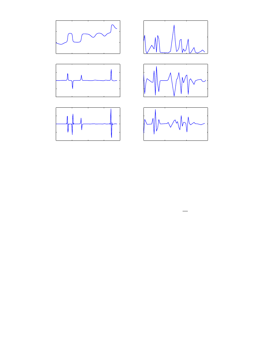
Figure 7.

The spatial and temporal vectors. In the left column, from top to bottom are θ and two spatial derivatives

c

(curvature) and ∆c respectively. In the right column, from top to bottom g), h) and i) are the temporal derivatives v

(velocity), ˙v (acceleration) and ¨

v

(jerk).

• a cubic spline smoothing interpolation that results in the curve (x

∗∗

i

, y

∗∗

i

). The only fixed points in this

interpolation are the beginning and ending points of the stroke, (x

1

, y

1

) and (x

n

, y

n

), respectively. The

length of the smoothed curve is denoted by s

∗∗

.

• A final uniform spatial re-sampling of the smoothed curve (x

∗∗

i

, y

∗∗

i

), leading to the curve points (x

′

i

, y

′

i

).

Associated with this vector is the path length vector, s

′

i

, i = 1, . . . , n

′

, n

′

=

s

∗∗

γ

, computed from points

(x

′

i

, y

′

i

) as in equation 1.

Figure 6 illustrates the preprocessing phase. In this figure, black dots (•) represent the original sampled points,
white dots (◦) correspond to the linearly interpolated points, and the continuous line is the resulting smoothed
data.

Spatial information

We define six vectors in the spatial domain over the smoothed, uniformly sampled curve

points (x

′

i

, y

′

i

):

• x

′

— horizontal coordinates.

• θ — angle of the path tangent with the x-axis.

• y

′

— vertical coordinates.

• c — curvature

• s

′

— path distance from the origin.

• ∆c — derivative of curvature in order to space.

The first three vectors were obtained during the smoothing process. The angle is calculated using equation

3 and 4, in order to create a continuous vector. The function arctan

∗

is the four quadrant arc-tangent of δx and

δy, with the domain [−π, π].

θ

i

= arctan

∗

µ δy

1

δx

1

¶

+

i

X

j=1

δθ

j

(3)

δθ

i

= min

½

δ arctan

∗

µ δy

i

δx

i

¶

+ 2kπ

¾

k ∈ Z

(4)

The curvature, c, is defined as c =

δθ
δs

, and is inversely proportional to the radius of the intrinsic circumference

that fits the point where the curvature is being calculated. The rate of change of curvature is defined by ∆c =

δc
δs

.

Figure 7, left column, presents an example of these vectors.

Temporal information

In the temporal domain we defined 9 vectors, calculated from the original acquired

data points:

• x — the vector with the input x

i

. . . x

n

values.

• v

x

— horizontal velocity.

• ˙v — tangential acceleration.

• y — the vector with the input y

i

. . . y

n

values.

• v

y

— vertical velocity.

• ¨v — tangential jerk.

• t — the input time vector t

i

. . . t

n

.

• v — tangential velocity.

• w — angular velocity.

The first three vectors are the acquired data from the pointing device, and serve as input for the processing

algorithms that lead to the time related features. The following vectors are several derivatives in order to time.
Equation 5 describes how these vectors are obtained. The vector θ

t

is calculated as in equation 3, but with

respect to time.

v

x

=

δx

δt

;

v

y

=

δy

δt

;

v =

q

v

2

x

+ v

2

y

;

˙v =

δv

δt

;

¨

v =

δ ˙v

δt

;

w =

δθ

t

δt

(5)

Feature generation

Each stroke is characterized by a feature vector, f , which contains relevant information

for the recognition system.

Feature extraction is based on the spatial and temporal vectors described before. The vectors x

′

, y

′

, θ, c, ∆c,

v

x

, v

y

, v, ˙v, ¨

v, and w are statistically analyzed, and 5 values are computed per vector: the minimum, maximum,

mean, standard deviation, and (maximum - minimum). This analysis produces the first 55 features, f

1

...f

55

.

Features f

56

= t

n

and f

57

= s

n−1

correspond, respectively, to the time duration and the length of the stroke.

Two other features are computed related to the path of the stroke. The straightness, (f

57

), is defined as the

ratio of the Euclidean distance between the starting and ending points of the stroke, and the total path distance:

straightness =

√

(x

1

−

x

n

)

2

+(y

1

−

y

n

)

2

s

n−1

. The jitter (f

58

) is related to the tremor in the user movement, and is

calculated analyzing the ratio between the original path length and the smoothed path length: jitter =

s

′
n′

s

n−1

The curvature vector is processed searching for high curvature points, that we call critical points. The

number of critical points (f

59

) is defined by n

critical points

=

P

n
i=1

z

i

, with z

i

=

½

1

if ∆c

i

= 0 ∧ |c

i

| > α

0

otherwise

.

We search for zeros in the derivative of c, and select the points that have absolute curvature higher than a
constant α =

π

10

rad

pixel

2

.

We consider a pause in the user interaction when two consecutive events are separated in time by more than

β=0.1 seconds. We compute the time to click (f

60

≡ time to click = t

n

− t

n−1

), the number of pauses (f

61

)

number of pauses =

n

X

i=1

p

i

, with p

i

=

½

1 if t

i

> β

0 otherwise

,

(6)

the paused time (f

62

≡ paused time =

P

n
i=1

p

i

t

i

), and the paused time ratio (f

63

≡ paused time ratio =

paused time

t

n

).

3.2. Feature Selection

The total set of features generated by the feature extraction procedure is analyzed in order to select a subset of
features that “best”discriminate among the several users.

For the purpose of feature selection we consider that we have a classifier system that receives a subset of the

features and returns the equal error rate of the system. The classifier will be explained in the subsection 3.3. We
searched for a set of features for each user. We used a greedy search

17, 18

algorithm, typically called Sequential

Forward Selection (SFS)

19

that selects the best single feature and then adds one feature at time to the vector of

previously selected features. The algorithm stops when the equal error rate does not decrease.

3.3. Sequential Classification

The classifier’s purpose is to decide if a user is who he claims to be, based on the patterns of interaction with
the computer.

We consider that the i

th

user is denoted by the class w

i

, i = 1, . . . , L, and L is the number of classes. As

defined before, a feature vector is associated with one stroke, the user interaction between two mouse clicks.
Given a sequence of n

s

consecutive strokes executed by the user, w

i

, interaction information is summarized in

the vector X = X

1

...X

n

s

, consisting of the concatenation of the feature vectors associated with each stroke.

X

j

= x

j
1

...x

j

n

fi

, the feature vector representing the jth stroke, has n

f

i

elements, n

f

i

being the number of features

identified for user w

i

in the feature selection phase.

Considering each stroke at a time, and assuming independence between strokes we can write

p(X|w

i

) =

n

s

Y

j=1

p(X

j

|w

i

).

(7)

The classifier will decide to accept or reject the claimed identity based on two distributions: the genuine

distribution p(X|w

i

), and the impostor distribution p(X| w

i

) that is based on a mixture of distributions (weibull

distributions), one for each other user not equal to i, expressed as p(X|w

i

) =

P

j6=i

[

1

L

p(X|w

i

)]. In the previous

equation we assume that the classes are equiprobable, p(w

i

) = 1/L

i = 1...L. We can therefore express the

posterior probability function as

p(w

i

|X) =

p(X|w

i

)

P

L
k=1

p(X|w

k

)

= 1 − p(w

i

|X).

(8)

Since p(w

i

|X) represents an estimate of the probability of the classification being correct, we establish a limit,

λ, to select one of the decisions, using the decision rule in equation 9. The value of λ is adjusted to operate in
the equal error rate point.

Accept(X ∈ w

i

) =

½

true

if p(w

i

|X) > λ

f alse otherwise

(9)

3.4. Learning

The learning phase consists of the estimation of the probability density functions of each user interaction, p(X|w

i

).

The collected data set was split in two parts, half of the data being used for learning (training set), and the
other half for estimating the performance of the system (testing set). As stated before we are assuming stroke
independence and thus we only need to learn the probability density function of a single stroke p(X

j

|w

i

) (where

X

j

is the feature vector of a stroke).

We tested two strategies for density estimation.

Multimodal non-parametric estimation

In a first attempt we used a non-parametric multi-modal model

based on Parzen density estimation.

20

A transformation expressed in equation 10 was applied to each feature

of the data x

j
i

(the i

th

feature of the feature vector of a stroke) normalizing the data in order to have zero mean

and unitary standard deviation for each feature. In equation 10, µ

i

is the mean and σ

i

is the standard deviation

of feature i estimated from the training set.

x

j
i

=

x

j
i

− µ

i

σ

i

(10)

Equation 11 expresses the probability density function obtained with the parzen windows method were X

j

is the pattern (stroke) for which we want to estimate the probability density, and X

j

i

is the i

th

element of the

training set for the user w

i

. We selected the normal density function as the kernel window K . Some tests were

performed to adjust the width of the window and the unitary standard deviation was selected (equation 12),
thus using Σ = I, the identity matrix, as the covariance matrix of the multimodal normal density function.

p

parzen

(X

j

|w

i

) =

1

n

n

X

i=1

K(X

j

− X

j

i

)

(11)

K(X) =

1

(2π)

n

fi

/2

exp(−

1
2

X

T

X)

(12)

Unimodal parametric estimation

In a second attemp we used a unimodal statistical model for the feature

vectors, assuming statistical independence between features. The estimation of p(X

j

|w

l

) can be done using the

independence assumption p(X

j

|w

l

) =

Q

i

p(x

j
i

|w

l

). We use as parametrical model for p(x

j
i

|w

l

) the weibull

21

distribution

p

weibull

(x|a, b) = abx

(b−1)

e

(−ax

b

)

.

(13)

Given the definition of skewness, skewness

i

=

E(x

i

−

µ

i

)

3

σ

3
i

, where µ

i

, σ

i

represent the mean value and standard

deviation, respectively, for feature i, consider the following sequence of data transformations:

if

skewness

i

< 0 ⇒ x

i

= −x

i

(14)

x

i

= x

i

− min(x

i

)

(15)

When performing these transformations on the data, the weibull distribution can approximately fit several
distributions, such as the exponential distribution (when b = 1) and normal distribution (when 0 ≪ µ < 1 ).

Given the data from one user and one feature, maximum likelihood estimates of the parameters a and b were

obtained.

4. RESULTS

The data set consists of approximately 10 hours of interaction recorded from 50 users, corresponding to more
than 400 strokes per user. In order to use the same number of strokes per user in the tests performed, we
randomly selected 400 strokes from each user. The set of strokes was divided into two equal parts, one for the
training phase and the other for the testing phase.

Using the training set we estimated the conditional density distributions, p(X

j

|w

i

), using both the multimodal

non-parametric form based on the method by Parzen, and the parametrical form (weibull distribution) based on
maximum likelihood estimation.

We then applied the feature selection step (see section 3.2) using the testing data set for selecting a different

combination of features for each user. The method was applied both using the multimodal nonparametric and
the unimodal parametric density estimates. Performance evaluation was based on the classification of sequences
with 10 strokes.

0

10

20

30

40

50

60

70

80

90

0

0.05

0.1

0.15

0.2

0.25

0.3

0.35

0.4

0.45

0.5

Equal error rate

time (s)

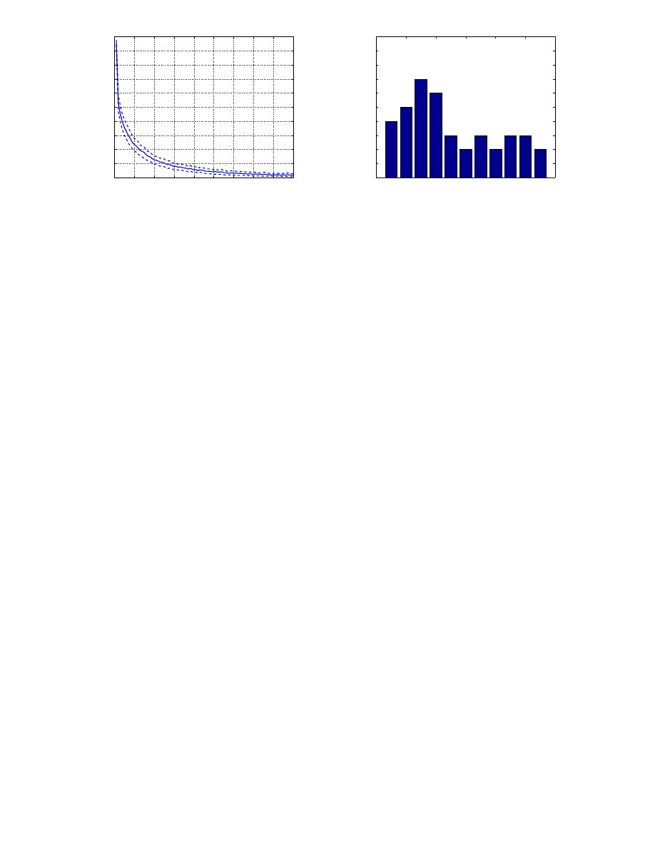
Figure 8.

Equal error rate results of the verification

system. The solid line is the mean of the equal error
rate of all users. The dashed lines are the mean plus
and minus half standard deviation.

0

2

4

6

8

10

12

0

1

2

3

4

5

6

7

8

9

10

Feature vector size

Number of users

Figure 9.

Histogram of the length of feature vectors,

computed over 25 users.

The equal error rate obtained with the two methods for density estimation was equivalent, without relevant

statistical differences. The set of features selected by both methods for each user was similar since half of the
features were common and most of the remaining were related. The size of the feature vector for both methods
was also similar for the same user. The relevant difference between the multimodal nonparametric and unimodal
parametric density estimation was in the time complexity. According to our tests, Parzen density estimation
was approximately 30-40 times slower than the parametric density estimation based on the weibull distribution.

When testing the system for one user, we consider an imposter as one of the other users. The test function

returns the equal error rate given N sequences of strokes of length l using the classifier tuned for user i. The
input sequence of strokes of a test is composed of N/2 strokes randomly sampled from the testing set of the user,
and N/2 strokes randomly sampled from the testing sets of all the other users.

One of the free variables of the system is the number of strokes that the system will use in the verification

task. Bootstrap

22

estimates of the system performance as a function of the sequence stroke length (from 1 to

100 strokes) was obtained using 10000 bootstrap samples from the test set. The mean duration of a stroke is
approximately 1 second. The values associated with the test using 10 strokes requires approximately 10 seconds
of interaction. In table 1 we present the mean results of the equal error rate for all 40 users for several stroke
sequence lengths. A graphical display of these results is shown in figure 8. As shown, the mean value and the
standard deviation of the EER progressively tends to zero as more strokes are added to the decision rule. This
illustrates the refinement of the performance obtained by the sequential classifier.

Almost all features were used (58 from the total of 63) and the vector of features has different lengths for the

different users, ranging from 1 to 11 features. The average size of the features vector is 5. The 5 most frequently
used features by the several users are: max(v

y

) (used by 21 users); min(v) (16 users); max(v

x

) − min(v

x

) (12

users); paused time (11 users); jitter (11 user). In figure 9 we present the histogram of the feature vector sizes
for all the users.

We also compared the performance of the system with different number of users. We tested the system with

10, 20, 30, 40 and 50 users using 30 strokes. The mean EER results obtained for all the users were similar
presenting no relevant correlation with the number of users.

Table 1.

Mean equal error rate (eer) and respective

standard deviation (std) for different stroke sequence
lengths (l).

l

eer

std

1

0.480

0.016

2

0.263

0.057

5

0.179

0.056

10

0.118

0.043

20

0.063

0.029

50

0.020

0.016

100

0.007

0.011

200

0.002

0.005

Table 2.

Comparison between several biometric tech-

niques.

Biometric technique

Equal Error Rate

Retinal Scan

1:10 000 000

Iris Scan

1:131 000

Fingerprints

1:500

Hand Geometry

1:500

Signature Dynamics

1:50

Voice Dynamics

1:50

30s of interaction

1:50

60s of interaction

1:100

90s of interaction

1:200

5. CONCLUSIONS

We have presented a novel user verification technique based on behavioural biometrics, extracted from human-
computer interaction through a pointing device. For the implementation of the proposed technique, a prototype
system, working on the world wide web, was developed. This system comprises a data acquisition module, respon-
sible for the collection of user interaction data, and a recognition module, that produces the user classification
and estimates of the performance of the decision rule.

The user authentication method applies a statistical classifier to the sequential data produced along the

interaction. A large set of features were initially extracted from the collected data, using both time domain
related and spatial information from the mouse movement patterns. This initial set was then reduced to a small
number of features by applying a feature selection algorithm. Using a greedy search, and taking the classifier
performance, measured by the EER, as objective function, feature selection was tuned for each user. A sequential
classifier was then designed to decide on the authenticity of the identity claim of users, based on the selected
features. The two strategies used for density estimation showed that we can assume feature independence and
base the system in a unimodal parametrical model.

Results using 30 seconds of user interaction by the proposed system are comparable to the performance of

some established behavioural biometric techniques. Table 2 presents EER values reported in the literature for
several biometric techniques.

23

The accumulated data from user interaction increase the system performance.

Tests with different number of used presented no influence in the mean equal error rate of the system.

Preliminary results show that the proposed technique is a promising tool for user authentication. Furthermore,

it is an inexpensive authentication technique, that uses standard human-computer interaction devices, and
remotely accesses user behavioural information through the world wide web.

REFERENCES

1. E. Bowman, “Everything you need to know about biometrics,” tech. rep., Identix Corporation,

http://www.ibia.org/EverythingAboutBiometrics.PDF, 2000.

2. A. Jain, R. Bolle, and S. Pankanti, Biometrics: Personal Identification in Networked Society, Kluwer Aca-

demic Publishers, 1999.

3. V. M. Jr and Z. Riha, “Biometric authentication systems,” Tech. Rep. FIMU-RS-2000-08, FI MU Report

Series, http://www.fi.muni.cz/informatics/reports/files/older/FIMU-RS-2000-08.pdf, 2000.

4. A. Jain, L. Hong, S. Pankanti, and R. Bolle, “An identity authentication system using fingerprints,” Pro-

ceedings of the IEEE 85(9), 1997.

5. S. Liu and M. Silverman, “A practical guide to biometric security technology,” ITProfessional 3(1), 2001.
6. T. Mansfield and G. Roethenbaugh, “1999 glossary of biometric terms,” tech. rep., Association for Biomet-

rics, http://www.afb.org.uk/downloads/glossary.pdf, 1999.

7. J. G. Daugman and G. O. Williams, “A proposed standard for biometrics decidability,” in Proceedings of

the CardTech/SecureTech Conference, Atlanta, 1996.

8. J. Gupta and A. McCabe, “A review of dynamic handwritten signature verification,” tech. rep., James Cook

University, Australia, http://citeseer.nj.nec.com/gupta97review.html, 1997.

9. R. Kashi, J. Hu, W. Nelson, and W. Turin, “On-line handwritten signature verification using hidden markov

model features,” in Proceedings of International Conference on Document Analysis and Recognition, 1997.

10. A. Jain, F. D. Griess, and S. D. Connell, “On-line signature verification,” Pattern Recognition 35(12), 2002.
11. M. F. BenZeghiba, H. Bourlard, and J. Mariethoz, “Speaker verification based on user-customized

password,” Tech. Rep. IDIAP-RR 01-13, Institut Dalle Molle d’Intelligence Artificial Perceprive,
http://www.idiap.ch/ marietho/publications/orig/rr01-13.ps.gz, 2001.

12. F. Monrose and A. D. Rubin, “Keystroke dynamics as a biometric for authentication,” Future Generation

Computer Systems 16(4), 2000.

13. H. Said, G. Peake, T. Tan, and K. Baker, “Writer identification from non-uniformly skewed handwriting

images,” in British Machine Vision Conference, 1998.

14. I. Jermyn, A. Mayer, F. Monrose, M. K. Reiter, and A. D. Rubin, “The design and analysis of graphical

passwords,” in Proceedings of the 8th USENIX Security Symposium, 1999.

15. H. Gamboa and A. Fred, “A User Authentication Technique Using a Web Interaction Monitoring System.

Proceedings of the 5

th

Iberian Conference on Pattern Recognition and Image analysis ,” 2003.

16. H. Gamboa and V. Ferreira, “WIDAM - Web Interaction Display and Monitoring. Proceedings of the 5

th

International Conference on Enterprise Information Systems,” 4, pp. 21–27, 2003.

17. S. Russell and P. Norvig., Artificial Intelligence: a modern approach, Prentice Hall, 1995.
18. W. Siedlencki and J. Sklansky, Handbook of Pattern Recognition and Computer Vision, ch. On Automatic

Feature Selection. World Scientific, 1993.

19. A. K. Jain, R. P. W. Duin, and J. Mao, “Statistical pattern recognition: A review,” IEEE Transactions on

Pattern Analysis and Machine Intelligence 22(1), 2000.

20. R. O. Duda, P. E. Hart, and D. G. Stork, Pattern Classification , John Wiley and Sons, 2001.
21. R. B. Abernethy, The New Weibull Handbook, Robert B. Abernethy, 2000.
22. B. Efron and R. J. Tibshirani, An Introduction to the Bootstrap, Chapman & Hall, 1993.
23. T. Ruggles, “Comparison of biometric techniques,” tech. rep., California Welfare Fraud Prevention System,

http://www.bio-tech-inc.com/bio.htm, 2002.