Filters Duch Chap3

Filter methods

Wlodzislaw Duch

Department of Informatics, Nicholaus Copernicus University,
Grudzi¸

adzka 5, 87-100 Toru´

n, Poland, and

Department of Computer Science, School of Computer Engineering,
Nanyang Technological University, Singapore 639798
Google: Duch

1 Introduction to filter methods for feature selection

Feature ranking and feature selection algorithms may roughly be divided into
three types. The ﬁrst type encompasses algorithms that are built into adaptive
systems for data analysis (predictors), for example feature selection that is a
part of embedded methods (such as neural training algorithms). Algorithms
of the second type are wrapped around predictors providing them subsets of
features and receiving their feedback (usually accuracy). These wrapper ap-
proaches are aimed at improving results of the speciﬁc predictors they work
with. Third type includes feature selection algorithms that are independent
of any predictors, ﬁltering out features that have little chance to be useful
in analysis of data. These ﬁlter methods are based on performance evalua-
tion metric calculated directly from the data, without direct feedback from
predictors that will ﬁnally be used on data with reduced number of features.
Such algorithms are usually computationally less expensive than those from
the ﬁrst or the second group. This chapter is devoted to ﬁlter methods.

The feature ﬁlter is a function returning a relevance index J(S|D, Y ) that

estimates, given the data

D, how relevant a given feature subset S is for the

task Y (usually classiﬁcation or approximation of the data). Since the data and
the task are usually ﬁxed and only the subsets

S vary the relevance index may

be written as J(S). In text classiﬁcation these indices are frequently called
“feature selection metrics” [18], although they may not have formal properties
required to call them a distance metric. Instead of a simple function (such as a
correlation or information content) some algorithmic procedure may be used
to estimate the relevance index (such as building of a decision tree or ﬁnding
nearest neighbors of vectors). This means that also a wrapper or an embedded
algorithm may be used to provide relevance estimation to a ﬁlter used with
another predictor.

Relevance indices may be computed for individual features X

, i = 1 . . . N ,

providing indices that establish a ranking order J(X

)

≤ J(X

)

· · · ≤

J(X

). Those features which have the lowest ranks are ﬁltered out. For inde-

pendent features this may be suﬃcient, but if features are correlated many of
important features may be redundant. Moreover, the best pair of features do
not have to include a single best one [47, 7]. Ranking does not guarantee that
the largest subset of important features will be found. Methods that search
for the best subset of features may use ﬁlters, wrappers or embedded feature
selection algorithms. Search methods are independent of the evaluation of fea-
ture subsets by ﬁlters, and are a topic of Chapter 5. The focus here is on ﬁlters
for ranking, with only a few remarks on calculation of relevance indices for
subsets of features presented in Sec. 8.

The value of the relevance index should be positively correlated with ac-

curacy of any reasonable predictor trained for a given task Y on the data D
using the feature subset

S. This may not always be true for all models, and on

the theoretical grounds it may be diﬃcult to argue which ﬁlter methods are
appropriate for a given data analysis model. There is little empirical experi-
ence in matching ﬁlters with classiﬁcation or approximation models. Perhaps
diﬀerent types of ﬁlters could be matched with diﬀerent types of predictors
but so far no theoretical arguments or strong empirical evidence has been
given to support such claim.

Although in the case of ﬁlter methods there is no direct dependence of

the relevance index on the predictors obviously the thresholds for feature
rejection may be set either for relevance indices, or by evaluation of the fea-
ture contributions by the ﬁnal system. Features are ranked by the ﬁlter, but
how many are ﬁnally taken may be determined using predictor as a wrap-
per. This “ﬁltrapper” approach is computationally less expensive than the
original wrapper approach because evaluation of predictor’s performance (for
example by a cross-validation test) is done only for a few pre-selected feature
sets. There are also theoretical arguments showing that this technique is less
prone to overﬁtting than pure wrapper methods [39]. In some data mining
applications (for example, analysis of large text corpora with noun phrases as
features) relatively inexpensive ﬁlter methods, with costs linear in the number
of features, may be prohibitively slow.

Filters, as all other feature selection methods, may be divided into local

and global types. Global evaluation of features takes into account all data
in a context-free way. Context dependence may include diﬀerent relevance for
diﬀerent tasks (classes), and diﬀerent relevance in diﬀerent areas of the feature
space. Local classiﬁcation methods, for example nearest neighbor methods
based on similarity, may beneﬁt more from local feature selection, or from
ﬁlters that are constructed on demand using only data from the neighborhood
of a given vector. Obviously taking too few data samples may lead to large
errors in estimations of any feature relevance index and the optimal tradeoﬀ
between introduction of context and the reliability of feature evaluation may
be diﬃcult to achieve. In any case the use of ﬁlter methods for feature selection
depends on the actual predictors used for data analysis.

In the next section general issues related to the ﬁlter methods are dis-

cussed. Section 3 is focused on the correlation based ﬁltering, Sec. 4 on rel-
evance indices based on distances between distributions and Sec. 5 on the
information theory. In Section 6 the use of decision trees for ranking as well
as feature selection is discussed. Reliability of calculation of diﬀerent indices
and bias in respect to the number of classes and feature values is very impor-
tant and is treated in Section 7. This is followed by some remarks in Sec. 8
on ﬁlters for evaluation of feature redundancy. The last section contains some
conclusions.

2 General issues related to filters

What does it mean that the feature is relevant to the given task? Artificial
Intelligence journal devoted in 1996 a special issue to the notion of relevance
(Vol. 97, no. 12). The common-sense notion of relevance has been rigorously
deﬁned in an axiomatic way (see the review in [3]). Although such deﬁnitions
may be useful for the design of ﬁlter algorithms a more practical approach
is followed here. Kohavi and John [30] give a simple and intuitive deﬁnition
of relevance that is suﬃcient for the purpose of feature selection: a feature
X is relevant in the process of distinguishing class Y = y from others if and
only if for some values X = x for which P(X = x) > 0 the conditional
probability

P(Y = y|X = x) is diﬀerent than the unconditional probability

P(Y = y). Moreover, a good feature should not be redundant, i.e. it should
not be correlated with other features already selected. These ideas may be
traced back to the test theory [19] developed for psychological measurements.

The main problem is how to calculate the strength of correlations between

features and classes (or more generally, between features and target, or out-
put, values), and between features themselves. The Bayesian point of view is
introduced below for the classiﬁcation problems, and many other approaches
to estimation of relevance indices are described in subsequent sections. Some
of these approaches may be used directly for regression problems, others may
require quantization of continuous outputs into a set of pseudo-classes.

Consider the simplest situation: a binary feature X with values x = {0, 1}

for a two class y = {+, −} problem. For feature X the joint probability P(y, x)
that carries full information about the relevance of this feature is a 2 by 2 ma-
trix. Summing this matrix over classes (“marginalizing”, as statisticians say)
the values of

P(x) probabilities are obtained, and summing over all feature

values x gives a priori class probabilities P(y). Because class probabilities
are ﬁxed for a given dataset and they sum to

P(y = +) + P(y = −) = 1

only two elements of the joint probability matrix are independent, for ex-
ample

P(y = −, x = 0) and P(y = +, x = 1). For convenience notation

P(y

, x

) =

P(y = i, x = j) is used below.

The expected accuracy of the majority classiﬁer (MC) A

= max

P(y)

is independent of the feature X because MC completely ignores informa-

tion about feature values. The Bayesian Classiﬁer (BC) makes optimal de-
cisions based on the maximum a posteriori probability: if x = x

then for

P(y

−

, x

) > P(y

, x

) class y

−

should always be selected, giving a larger frac-

tion

P(y

−

, x

) of correct predictions, and smaller fraction

P(y

, x

) of errors.

This is equivalent to the Maximum-a-Posteriori (MAP) rule: given X = x se-
lect class that has greater posterior probability

P(y|x) = P(y, x)/P(x). Bayes

error is given by the average accuracy of the Bayesian Classﬁer (BC) using
MAP, or “informed majority classiﬁer” using a single feature X is:

(X) =

j=0,1

max

P(y

, x

) =

j=0,1

max

P(x

)

P(y

(1)

Precise calculation of “real” joint probabilities

P(y

, x

) or the conditional

probabilities

P(x

) using observed frequencies requires an inﬁnite amount

of the training data, therefore such Bayesian formulas are strictly true only
in the asymptotic sense. The training set should be a large, random sample
that represents distribution of data in the whole feature space.

Because A

(X) ≤ A

(X) ≤ 1, a Bayesian relevance index scaled for

convenience to the [0, 1] interval may be taken as:

(X) = (A

(X) − A

(X))/(1 − A

(X)) ∈ [0, 1].

(2)

The J

(X) may also be called “a purity index”, because it indicates how

pure are the discretization bins for diﬀerent feature values (intervals). This
index is also called “the misclassiﬁcations impurity” index, and is sometimes
used to evaluate nodes in decision trees [16].

Two features with the same relevance index J

(X) = J

) may be

ranked as equal, although their joint probability distributions

P(y

, x

) may

signiﬁcantly diﬀer. Suppose that

P(y

−

) > P(y

) for some feature X, there-

fore A

(X) = P(y

−

). For all distributions with

P(y

−

, x

) > P(y

, x

)

and

P(y

, x

) > P(y

−

, x

) accuracy of Bayesian classiﬁer is A

(X) =

P(y

−

, x

P(y

, x

), and the error is

P(y

, x

P(y

−

, x

) = 1

−A

(X). As

long as these equalities and inequalities between joint probabilities hold (and
P(y

, x

)

≥ 0) two of the probabilities may change, for example P(y

, x

) and

P(y

, x

), without inﬂuencing A

(X) and J

(X) values. Thus Bayesian

relevance index is not suﬃcient to uniquely rank features even in the simplest,
binary case. In fact most relevance indices cannot do that without additional
conditions (see also Sec. 7).

This reasoning may be extended to multi-valued features (or continuous

features after discretization [35]), and multi-class problems, leading to proba-
bility distributions that give identical J

values. The expected accuracy of a

Bayesian classiﬁcation rule is only one of several aspects that could be taken
into account in assessment of such indices. In the statistical and pattern recog-
nition literature various measures of inaccuracy (error rates, discriminability),
imprecision (validity, reliability), inseparability and resemblance (resolution,
reﬁnement) are used (see [22, 14] for extended discussion). Knowing the joint

P(y, x) probabilities and using the MAP Bayesian Classiﬁer rule confusion
matrices

F(y

, y

) may easily be constructed for each feature, repre-

senting the joint probability of predicting class y

when the true class is y

F (true, predicted) =

+−

−+

−−

TP FN
FP TN

(3)

where

is called a hit or true positive (TP) rate;

−−

is a hit or true

negative (TN) rate;

−+

is a false alarm, or false positive (FP) rate (for

example, healthy person predicted as sick), and

+−

is a miss, or false negative

(FN) rate (sick person predicted as healthy).

Confusion matrices have only two independent entries because each row

has to sum to

−j

P(y

), the a priori true class probability

(estimated as the fraction of all samples that belong to the class y

). In

medical informatics it is common to use as the two independent variables
combinations known as sensitivity (recall, detection, or true positive rate)
S

/P(y

) =

F(y

) and speciﬁcity S

−

−−

/P(y

−

) =

F(y

−

that is a proportion of samples from the ﬁrst (second) class that are classiﬁed
correctly. They reﬂect the type of errors that the predictor makes and are
diagonal elements of the confusion matrix based on conditional probabilities
F(y

), with entries in each row summing to 1. For example, sensitivity

shows how well sick people (class y = +) are correctly recognized by classiﬁ-
cation rule based on some feature (results of a medical test), and speciﬁcity
shows how well healthy people (class y = −) are recognized as healthy by
the same test. Arithmetic average of these two quantities is called a balanced
accuracy

Acc

(

F(y

) +

F(y

−

)),

(4)

and is particularly useful for unbalanced datasets. Standard accuracy, the sum
of true positive and true negative probabilities, is of course obtained by weight-
ing with class probabilities Acc =

F(y

, y

) +

F(y

−

, y

−

) =

F(y

)

P(y

) +

F(y

−

)

P(y

−

). For feature ranking using accuracy-based relevance indices,

such as the A

, J

indices, is equivalent to comparing

F(y

, y

)

−F(y

, y

−

)

(true positives minus false positives), while using balanced accuracy is equiva-
lent to

F(y

)

− F(y

−

) (true positives ratio minus false positives ratio),

because terms that are constant for a given data will cancel during compari-
son. This diﬀerence may be rescaled, for example by using [18]:

BN S = G

−1

(

F(y

))

− G

−1

(

F(y

−

))

(5)

where G

−1

(

·) is the z-score, or the standard inverse cumulative probability

function of a normal distribution. This index, called bi-normal separation
index, worked particularly well in information retrieval (IR) [18]. Another
simple criterion that is frequently used in this ﬁeld is called the Odds Ratio:

Odds =

F(y

)

F(y

−

)

F(y

−

)

F(y

−

)

F(y

)(1

− F(y

−

)

− F(y

))

F(y

−

)

(6)

where zero probabilities are replaced by small positive numbers.

Ranking of features may be based on some combination of sensitivity and

speciﬁcity. Costs of not recognizing a sick person (low sensitivity) may be
much higher than cost of temporary hospitalization (low speciﬁcity). Costs of
misclassiﬁcation may also be introduced by giving a factor to specify that

+−

type of errors (false positive) are α times more important than F

−+

type of

errors (false negative). Thus instead of just summing the number of errors the
total misclassiﬁcation cost is E(α) = αF

−+

+−

. For binary feature values

the BC decision rule has no parameters, and costs E(α) are ﬁxed for a given
dataset. However, if the

P(y, x) probabilities are calculated by discretization of

some continuous variable z so that the binary value x = Θ(z − θ) is calculated
using a step functionΘ, the values of sensitivity F(y

; θ) and speciﬁcity

F(y

−

; θ) depend on the threshold θ, and the total misclassiﬁcation cost

E(α, θ) can be optimized with respect to θ.

A popular way to optimize such thresholds (called also “operating points”

of classiﬁers) is to use the receiver operator characteristic (ROC) curves
[22, 44]. These curves show points R(θ) = (F(y

−

; θ), F(y

; θ)) that

represent a tradeoﬀ between the false alarm rate

F(y

−

; θ) and sensitiv-

ity

F(y

; θ) (true positives rate). The Area Under the ROC curve (called

AUC) is frequently used as a single parameter characterizing the quality of
the classiﬁer [23], and may be used as a relevance index for BC or other clas-
siﬁcation rules. For a single threshold (binary features) only one point R =
(

F(y

−

), F(y

)) is deﬁned, and the curve has a line segment connecting

it with points (0, 0) and (1, 1). In this case AUC=

(

F(y

) +

F(y

−

)) is

simply equal to the balanced accuracy, ranking as identical all features that
have the same diﬀerence between true positive and false positive ratios. In
general this will not be the case and comparison of AUCs may give a unique
ranking of features. In some applications (for example, in information re-
trieval) classiﬁers may have to work at diﬀerent operating points, depending
on the resources that may change with time. Optimization of ROC curves
from the point of view of feature selection leads to ﬁltering methods that may
be appropriate for diﬀerent operating conditions [6].

A number of relevance indices based on modiﬁed Bayesian rules may be

constructed, facilitating feature selection not only from the accuracy, but also
from the cost or conﬁdence point of view. The confusion matrix

F(y

, y

) for

the two-class problems may be used to derive various combinations of accuracy
and error terms, such as the harmonic mean of recall and precision called the
F -measure,

(X) = 2/(1 + F

−−

− F

(7)

popular and well-justiﬁed in information retrieval (IR) [49]. Selection of the
AUC or balanced accuracy instead of the standard accuracy corresponds to a
selection of the relative cost factor α = P(y

−

)/P(y

) [14]. An index combining

the accuracy and the error term J(γ) = F

−−

− γ(F

−+

+−

) =

A − γE does not favor one type of errors over another, but it may be used

to optimize conﬁdence and rejection rates of logical rules [13]. For γ = 0 this
leads to the A

Bayesian accuracy index, but for large γ a classiﬁcation

rule that maximizes J(γ) may reduce errors increasing conﬁdence in the rule
at the expense of leaving some samples unclassiﬁed. Non-zero rejection rates
are introduced if only signiﬁcant diﬀerences between the

P(y, x) values for

diﬀerent classes are kept, for example the feature is not ranked (rejected) if
|P(y

, x) − P(y

−

, x)| < θ for all values of x.

From the Bayesian perspective one cannot improve the result of the max-

imum a posteriori rule, so why is the J

(X) index rarely (if ever) used, and

why are other relevance indices used instead? There are numerous theoretical
results [11, 1] showing that for any method of probability density estimations
from ﬁnite samples convergence may be very slow and no Bayes error estimate
can be trusted. Reliability of

P(y, x) estimates rapidly decreases with a grow-

ing number of distinct feature values (or continuous values), growing number
of classes, and decreasing number of training samples per class or per feature
value. Two features with the same J

(X) index may have rather diﬀer-

ent distributions, but the one with lower entropy may be preferred. Therefore
methods that compare distributions of feature and class values may have some
advantages [46]. Empirical study of simple relevance indices for text classiﬁca-
tion shows [18] that accuracy is rather a poor choice, with balanced accuracy
(equivalent to comparison of AUCs for the two-class problems) giving much
higher recall at similar precision. This is not surprising remembering that in
the applications to text classiﬁcation the number of classes is high and the
data are very unbalanced (

P(y

) is very small).

Similarity of distributions may be estimated using various distance mea-

sures, information theory, correlation (dependency) coeﬃcients and consis-
tency measures, discussed in the sections below. Some theoretical results re-
lating various measures to the expected errors of the Bayesian Classiﬁer have
been derived [50, 48] but theoretical approaches have met only with limited
success and empirical comparisons are still missing. Features with continuous
values should be discretized to estimate probabilities needed to compute rele-
vance indices [36, 35]. Alternatively, the data may be ﬁtted to a combination
of some continuous one-dimensional kernel functions, for example Gaussian
functions, and integration may be used instead of summation.

Relevance indices J(X) introduced above are global or context-free, eval-

uating average usefulness of a single feature X. This may be suﬃcient in
many applications, but for some data distributions and for complex domains
features may be highly relevant in one area of the feature space and not rel-
evant at all in some other area. Some feature selection algorithms (such as
Relief described below) use local information, but calculate global, averaged
indices. Decision trees and other classiﬁcation algorithms that use the “divide
and conquer” approach hierarchically partitioning the whole feature space,
need diﬀerent subsets of features at diﬀerent stages. Restricting calculations
to the neighborhood O(x) of some input vector x, local or context-dependent,
relevance indices J(X, O(x)) are computed.

In mutliclass problems or in regression problems features that are impor-

tant for speciﬁc target values (“local” in the output space) should be rec-
ognized. For example, if the data is strongly unbalanced features that are
important for discrimination of the classes with small number of samples may
be missed. In this case the simplest solution is to apply ﬁlters to multiple
two-class problems. In case of regression problems ﬁlters may be applied to
samples that give target values in a speciﬁc range.

3 Correlation-based filters

Correlation coeﬃcients are perhaps the simplest approach to feature rele-
vance measurements. In contrast with information theoretic and decision tree
approaches they avoid problems with probability density estimation and dis-
cretization of continuous features and therefore are treated ﬁrst.

In statistics “contingency tables” deﬁned for pairs of nominal features

X, Y are frequently analyzed to determine correlations between variables.
They contain the numbers of times M

= N (y

, x

) objects with feature

values Y = y

, X = x

appear in a database. In feature selection m train-

ing samples may be divided into subsets of M

samples that belong to class

, i = 1 . . . K and have a speciﬁc feature value x

; summing over rows of the

matrix x distribution M

i·

of samples over classes is obtained, and sum-

ming over columns y distribution of samples M

·j

over distinct feature values

is obtained. The strength of association between variables X, Y is usually

measured using χ

statistics:

− m

)

, where m

= M

i·

·j

/m,

(8)

Here m

represent the expected number of observations assuming X, Y in-

dependence. Terms with m

= 0 should obviously be avoided (using suﬃcient

data to have non-zero counts for number of samples in each class and each fea-
ture value), or replaced by a small number. If feature and target values were
completely independent m

= M

is expected, thus large diﬀerences show

strong dependence. To estimate the signiﬁcance of the χ

test an incomplete

gamma function Q(χ

|ν) is used [40]. The number of degrees of freedom ν is

set to K − 1. This approach is justiﬁed from statistical point of view only if
the number of classes or the number of feature values are large. In contrast
to the Bayesian indices χ

results depend not only on the joint probabilities

Pr(x

, y

) = N (x

, y

)/m, but also on the number of samples m, implicitly

including the intuition that estimation of probabilities from small samples
is not accurate and thus the signiﬁcance of small correlations is rather low.
χ

statistics has been used in several discretization methods combined with

feature selection [36, 35].

The linear correlation coeﬃcient of Pearson is very popular in statistics

[40]. For feature X with values x and classes Y with values y treated as random

variables it is deﬁned as

(X, Y ) =

E(XY ) − E(X)E(Y )

(X)σ

(Y )

− ¯x

)(y

− ¯y

)

− ¯x

)

− ¯y

)

(9)

(X, Y ) is equal to ±1 if X and Y are linearly dependent and zero if they are
completely uncorrelated. Some features may be correlated positively, and some
negatively. This coeﬃcient can be applied to all types of numerical features
and targets. Even simpler criterion is based on separation of the means of the
class distributions:

µ(X, Y ) =

µ(y

)

− µ(y

−

)

(σ(y

) + σ(y

−

))

(10)

where µ(y

) is the mean value for class y

vectors and σ(y

) is the variance for

this class. For continuous targets a threshold y < θ divides vectors into y

and

−

groups. The square of this coeﬃcient is equal to the ratio of between-class

to within-class variances, known as the Fisher criterion [16]. The T-statistics
uses slightly diﬀerent denominator:

T (X, Y ) =

µ(y

)

− µ(y

−

)

σ(y

)

+ σ(y

−

)

−

(11)

where m

is the number of samples in class y

. For ranking absolute values

|(X, Y )|, |µ(X, Y )| and |T (X, Y )| are taken. How signiﬁcant are diﬀerences
in the (X, Y ) and other index values? The simplest test estimating the prob-
ability that the two variables are correlated is [40]:

P(X ∼ Y ) = erf

|(X, Y )|

m/2

(12)

where erf is the error function. Thus for m = 1000 samples linear correlations
coeﬃcients as small as 0.02 lead to probabilities of correlation around 0.5.
This estimation may be improved if the joint probability of X, Y variables is
binormal. The feature list ordered by decreasing values (descending order) of
the

P(X ∼ Y ) may serve as feature ranking. A similar approach is also taken

with χ

, but the problem in both cases is that for larger values of χ

or corre-

lation coeﬃcient probability

P(X ∼ Y ) is so close to 1 that ranking becomes

impossible due to the ﬁnite numerical accuracy of computations. Therefore
initial threshold for

P(X ∼ Y ) may be used in ranking only to determine how

many features are worth keeping, although more reliable estimations may be
done using cross-validation or wrapper approaches. An alternative is to use
a permutation test, computationally expensive but improving accuracy for
small number of samples [8] (see also Neal and Zhang, this volume).

If a group of k features has already been selected, correlation coeﬃcients

may be used to estimate correlation between this group and the class, includ-
ing inter-correlations between the features. Relevance of a group of features
grows with the correlation between features and classes, and decreases with

the growing inter-correlation. These ideas have been discussed in theory of
psychological measurements [19] and in the literature on decision making and
aggregating opinions [24]. Denoting the average correlation coeﬃcient between
these features and the output variables as r

= ¯

, Y ) and the average

between diﬀerent features as r

= ¯

, X

) the group correlation coeﬃcient

measuring the relevance of the feature subset may be deﬁned as:

J(X

, Y ) =

k + (k − 1)r

(13)

This formula is obtained from Pearsons correlation coeﬃcient with all vari-
ables standardized. It has been used in the Correlation-based Feature Selec-
tion (CFS) algorithm [21] adding (forward selection) or deleting (backward
selection) one feature at a time.

Non-parametric, or Spearman’s rank correlation coeﬃcients may be useful

for ordinal data types. Other statistical tests of independence that could be
used to deﬁne relevance indices, such as the Kolmogorov-Smirnov test based
on cumulative distributions and G-statistics[40].

A family of algorithms called Relief [42] are based on the feature weight-

ing, estimating how well the value of a given feature helps to distinguish
between instances that are near to each other. For a randomly selected sam-
ple x two nearest neighbors, x

from the same class, and x

from a diﬀerent

class, are found. The feature weight, or the Relief relevance index J

(X)

for the feature X, is increased by a small amount proportional to the diﬀer-
ence

|X(x) − X(x

)

| because relevance should grow for features that separate

vectors from diﬀerent classes, and is decreased by a small amount propor-
tional to

|X(x) − X(x

)

| because relevance should decrease for feature values

that are diﬀerent from features of nearby vectors from the same class. Thus
J

(X) ← J

(X) + η(|X(x) − X(x

)

| − |X(x) − X(x

)

|), where η is of the

order of 1/m. After a large number of iterations this index captures local
correlations between feature values and their ability to help in discrimination
of vectors from diﬀerent classes. Variants include ratio of the average over all
examples of the distance to the nearest miss and the average distance to the
nearest hit, that self-normalizes the results [28]:

(X) =

(

|X(x) − X(x

)

E(|X(x) − X(x

)

(14)

The ReliefF algorithm has been designed for multiclass problems and is

based on the k nearest neighbors from the same class, and the same number
of vectors from diﬀerent classes. It is more robust in presence of noise in
the data, and includes an interesting approach to estimation of the missing
values. Relief algorithms represent quite original approach to feature selection,
that is not based on evaluation of one-dimensional probability distributions
[42]. Finding nearest neighbors assures that the feature weights are context
sensitive, but are still global indices (see also [27] for another algorithm of the

same type). Removing context sensitivity (which is equivalent to assuming
an independence of features) makes it possible to provide a rather complex
formula for ReliefX:

(Y, X) =

GSx

− Sy)Sy

;

where

Sx =

i=1

P(x

)

;

Sy =

j=1

P(y

)

(15)

G =

P(y

)(1

− P(y

))

−

i=1


P(x

)

P(y

)(1

− P(y

))


 .

The last term is a modiﬁed Gini index (Sec. 6). Hall [21] has used a sym-

metrized version of J

(Y, X) index (exchanging x and y and averaging) for

evaluation of correlation between pairs of features. Relief has also been com-
bined with a useful technique based on the successive Gram-Schmidt ortogo-
nalization of features to the subset of features already created [28]. Connection
to the Modiﬁed Value Diﬀerence Metric (MVDM) is mentioned in the next
section.

4 Relevance indices based on distances between
distributions

There are many ways to measure dependence between the features and classes
based on evaluation of diﬀerences between probability distributions. A simple
measure – a diﬀerence between the joint and the product distributions – has
been proposed by Kolmogorov:

(Y, X) =

j=1

|P(y

, x

)

− P(x

)

P(y

)

(16)

This is very similar to the χ

statistics except that the results do not depend on

the number of samples. After replacing summation by integration this formula
may be easily applied to the continuous features, if probability densities are
known or some kernel functions have been ﬁtted to the data. It may reach
zero for completely irrelevant features, and it is bounded from above:

≤ D

(Y, X) ≤ 1 −

P(x

)

(17)

if correlation between classes and feature values is perfect. Therefore this index
is easily rescaled to the [0, 1] interval. For two classes with the same a priori
probabilities it reduces to:

(Y, X) =

|P(x

|y = 0) − P(x

|y = 1)|.

(18)

The quantity on the right side of Eq. 17 is known as the average Euclidean

norm of the conditional distribution, also called the Bayesian measure [48]:

(Y, X) =

j=1

P(y

)

(19)

It measures concentration of the conditional probability distribution and in
context of the feature selection, and is equivalent to the Gini index (Eq. 39)
used in decision trees (Sec. 6).

The Kullback-Leibler divergence:

((

P(X)||(P(Y )) =

) log

)

≥ 0,

(20)

is used very frequently, although it is not a distance (it is not symmetric). KL
divergence may be applied to relevance estimation in the same way as the χ

statistics:

(

P(X, Y )||P(X)P(Y )) =

j=1

P(y

, x

) log

P(y

, x

)

P(x

)

P(y

)

(21)

This quantity is also known as “mutual information” M I(Y, X). Kullback-
Liebler measure is additive for statistically independent features. It is sensitive
to the small diﬀerences in tail distributions, which may lead to problems,
especially in multiclass applications where the relevance index is taken as the
average value of KL divergences between all pairs of classes.

Jeﬀreys-Matusita distance (JM-distance) provides a more robust criterion:

(Y, X) =

j=1

P(y

, x

)

−

P(x

)

P(y

)

(22)

For Gaussian distributions D

is related to the Bhattacharya distance. Be-

cause D

≤ 2(1 − exp(−D

/8)) an exponential transformation J

− exp(−D

/8) is sometimes deﬁned, reaching zero for irrelevant features

and growing to 1 for a very large divergences, or highly relevant features.
There is some evidence that these distances are quite eﬀective in remote sens-
ing applications [5].

The Vajda entropy is deﬁned as [48]:

(Y, X) =

j=1

P(y

)(1

− P(y

)),

(23)

and is simply equal to the J

= 1

− J

. The error rate of the Bayesian

Classiﬁer is bounded by the Vajda entropy, A

(X) ≤ J

(Y, X). Although

many other ways to compare distributions may be devised they may serve as
better relevance indicators only if a tighter error bounds could be established.

In the memory-based reasoning the distance between two vectors X, X

with discrete elements (nominal or discretized), in a K class problem, is com-
puted using conditional probabilities [51]:

V DM (X, X

; Y )

j=1

|P(y

)

− P(y

)

(24)

This formula may be used to evaluate feature similarity when redundant

features are searched for.

5 Relevance measures based on information theory

Information theory indices are most frequently used for feature evaluation.
Information (negative of entropy) contained in the class distribution is:

H(Y ) = −

i=1

P(y

) log

P(y

(25)

where

P(y

) = m

/m is the fraction of samples x from class y

, i = 1..K.

The same formula is used to calculate information contained in the discrete
distribution of feature X values:

H(X) = −

P(x

) log

P(x

(26)

Continuous features are discretized (binned) to compute information associ-
ated with a single feature or some kernel functions are ﬁtted to approximate
the density of X values and integration performed instead of summation. In-
formation contained in the joint distribution of classes and features, summed
over all classes, gives an estimation of the importance of the feature. Informa-
tion contained in the joint distribution is:

H(Y, X) = −

j=1

P(y

, x

) log

P(y

, x

(27)

or for continuous features:

H(Y, X) = −

j=1

P(y

, x) log

P(y

, x)dx,

(28)

where

P(y

, x

), j = 1 . . . K is the joint probability (density for continuous

features) of ﬁnding the feature value X = x

for vectors x that belong to

some class y

and

P(x

) is the probability (density) of ﬁnding vectors with

feature value X = x

. Low values of H(Y, X) indicate that vectors from a

single class dominate in some intervals, making the feature more valuable for
prediction.

Information is additive for the independent random variables. The diﬀer-

ence M I(Y, X) = H(Y )+H(X)−H(Y, X) may therefore be taken as “mutual
information” or “information gain”. Mutual information is equal to the ex-
pected value of the ratio of the joint to the product probability distribution,
that is to the Kullback-Leibler divergence:

M I(Y, X) = −

i,j

P(y

, x

) log

P(y

, x

)

P(y

)

P(x

)

= D

(

P(y

, x

)

|P(y

)

P(x

)).

(29)

A feature is more important if the mutual information M I(Y, X) between
the target and the feature distributions is larger. Decision trees use closely
related quantity called “information gain” IG(Y, X). In the context of fea-
ture selection this gain is simply the diﬀerence IG(Y, X) = H(Y ) − H(Y |X)
between information contained in the class distribution H(Y ), and infor-
mation after the distribution of feature values is taken into account, that
is the conditional information H(Y |X). This is equal to M I(Y, X) because
H(Y |X) = H(Y, X) − H(X). A standard formula for the information gain is
easily obtained from the deﬁnition of conditional information:

IG(Y, X) = H(Y ) − H(Y |X) = H(Y ) +

P(y

, x

) log

P(y

) (30)

= H(Y ) −

P(x

) [

−P(y

) log

P(y

)] ,

where the last term is the total information in class distributions for subsets
induced by the feature values x

, weighted by the fractions

P(x

) of the number

of samples that have the feature value X = x

. Splits induced by tests in nodes

of decision trees are usually not based directly on all attribute values and thus
information gain in general is diﬀerent than mutual information, but for the
feature selection purposes these two quantities are identical.

It is not diﬃcult to prove that the Bayes error A

is bounded from above

by half of the value of the conditional information and from below by the
Fano inequality,

H(Y |X) − 1

log

≤ A

≤

H(Y |X),

(31)

although the left side is usually negative and thus not useful. Minimizing
H(Y |X) = H(Y ) − M I(Y, X), or maximizing mutual information, leads to

an approximation of Bayes errors and optimal predictions. Error bounds are
also known for Renyi entropy that is somehow easier to estimate in on-line
learning than the Shannon entropy [17].

Various modiﬁcations of the information gain have been considered in

the literature on decision trees (cf. [41]), aimed at avoiding bias towards the
multivalued features. These modiﬁcations include:

the information gain ratio IGR(Y, X) = M I(Y, X)/H(X),

(32)

the entropy distance

(Y, X) = 2H(Y, X) − H(Y ) − H(X), (33)

the Mantaras distance [10] D

(Y, X) = 1 − M I(Y, X)/H(Y, X),

(34)

and the Symmetrical Uncertainty coeﬃcient:

(Y, X) = 1 −

(Y, X)

H(Y ) + H(X)

= 2

M I(Y, X)

H(Y ) + H(X)

∈ [0, 1].

(35)

The J

coeﬃcient seems to be particularly useful due to its simplicity

and low bias for multi-valued features [21].

The J-measure:

(X) =

P(x

)

P(y

) log

P(y

)

P(y

)

(36)

has been initially introduced to measure information content of logical rules
[43], but it is applicable also to the feature selection [31].

Michie [37] has deﬁned an index called “average weight of evidence”, based

on plausibility, an alternative to entropy in information:

W E

(X) =

j=1

P(x

)

log

P(y

)(1

− P(y

))

− P(y

))

P(y

)

(37)

Minimum Description Length (MDL) is a general idea based on the Oc-

ckam’s razor principle and Kolmogorov’s algorithmic complexity [34]. Joint
complexity of theory inferred from the data and the length of the data encoded
using this theory should be minimal. MDL has been applied to the construc-
tion of decision trees and the selection of features [31]. As in the description
of χ

test m training samples are divided into subsets of M

samples that be-

long to class y

, j = 1 . . . K and have a speciﬁc feature value x

, i = 1 . . . M

The number of bits needed for optimal encoding of the information about the
class distribution for m training samples is estimated (this number is ﬁxed
for a given dataset), and the same estimation is repeated for each partition-
ing created by a feature value (or interval) x. Combinatorics applied to the
information coding leads to the MDL formula expressed using binomial and
multinomial coeﬃcients m!/m

! . . . m

! in the following way [31, 21]:

M DL(Y, X) = log

1·

! . . . M

K·

+ log

m + K − 1

K − 1

(38)

−

j=1

log

·j

+ K − 1

K − 1

−

j=1

log

·j

! . . . M

where M

i·

and M

·j

are marginal distributions calculated from the M

matrix.

The ﬁnal relevance index J

MDL

(Y, X) ∈ [0, 1] is obtained by dividing this

value by the ﬁrst two terms representing the length of the class distribution
description. A symmetrized version of MDL relevance index is used in [21],
calculated by exchanging features and classes and averaging over the two
values.

6 Decision trees for filtering

Decision trees select relevant features using top-down, hierarchical partition-
ing schemes. In the deeper branches of a tree only small portion of all data
is used and only local information is preserved. In feature selection global
relevance is of greater importance. One way to achieve it is to create a single-
level tree (for algorithms that allow for multiple splits), or a tree based on a
single feature (for algorithms that use binary splits only) and evaluate their
accuracy. An additional beneﬁt of using decision trees for continuous features
is that they provide optimized split points, dividing feature values into rela-
tively pure bins. Calculation of probabilities

P(x

) and

P(y

) needed for

estimation of mutual information and other relevance indices becomes more
accurate than with the naive discretization based on the bins of equal width
or bins with equal number of samples. Mutual information calculated after
discretization based on a decision tree may be a few times larger than using
naive discretization [15].

The 1R decision tree algorithm [26] is most appropriate for feature ﬁltering

because it creates only single level trees. Features are analyzed searching for
a subset of values or a range of values for which vectors from a single class
dominate. The algorithm has one parameter (called the “bucket size”), an
acceptable level of impurity for each range of the feature values, allowing for
reduction of the number of created intervals. Performance may be estimated
using the J

(Y, X) index, and the optimal bucket size may be evaluated

using cross-validation or bootstrap sampling that can help to avoid the bias
for large number of intervals but will also increase computational costs.

The C4.5 tree [41] uses information gain to determine the splits and to se-

lect most important features, therefore it always ranks as the most important
features that are close to the root node. The CHAID decision tree algorithm
[29] measures association between classes and feature values using χ

values,

as in Eq. 8. Although the information gain and the χ

have already been

mentioned as relevance indices the advantage of using decision trees is that
automatic discretization of continuous features is performed.

The Gini impurity index used in the CART decision trees [4] sums the

squares of the class probability distribution for a tree node, JGini(Y ) = 1 −

P(y

)

. Given a feature X a split into subsets with discrete feature values

(or values in some interval) may be generated and Gini indices in such

subsets calculated. This is equivalent to the calculation of the sum of squares
of all conditional probabilities:

JGini(Y, X) =

P(y

)

∈ [0, 1],

(39)

giving a measure of the probability concentration useful for feature ranking.
This index is similar to the entropy of class distributions and identical with
the Bayesian measure Eq. 19.

The Separability Split Value (SSV) criterion is used to determine splits in

decision tree [20] and to discretize continuous features [14, 12], creating a small
number of intervals (or subsets) with high information content. It may also be
used as the feature relevance index. The best “split value” should separate the
maximum number of pairs of vectors from diﬀerent classes. Among all split
values that satisfy this condition, the one that separates the smallest number
of pairs of vectors belonging to the same class is selected. The split value for
a continuous feature X is a real number s, while for a discrete feature it is a
subset of all possible values of the feature. In all cases, the left side (LS) and
the right side (RS) of a split value s is deﬁned by a test f (X, s) for a given
dataset

LS(s, f, D) = {x ∈ D : f (x, s) = T }}
RS(s, f, D) = D − LS(s, f, D),

(40)

where the typical test f (x, s) is true if the selected feature x

< s or (for

discrete feature) x

∈ {s}. The separability of a split value s is deﬁned for a

given test f as:

SSV(s, f ) = 2

i=1

|LS(s, f, D

)

| · |RS(s, f, D − D

)

(41)

−

min (

|LS(s, f, D

)

|, |RS(s, f, D

)

|) ,

where

is the subset of

D vectors that belong to the class k. If several

features separate the same number of pairs of training vectors the second
term ranks higher the one that separates a lower number of pairs from the
same class. This index has smilar properties to Gini and is easily calculated
for both continuous and discrete features. For 10 or less feature values all
subsets are checked to determine the simplest groupings, for larger number
of unique values the feature is treated as ordered and the best split intervals
are searched for. In the feature selection applications of the SSV, splits are
calculated and applied recursively to the data subsets

, creating a single-

feature tree. When pure nodes are obtained the algorithm stops and prunes the

tree. The Bayesian Classiﬁer rule is applied in each interval or for each subset
created by this algorithm to calculate the J

SSV

(Y, X) relevance index. More

complex tree-based approaches to determine feature relevance use pruning
techniques [14].

7 Reliability and bias of relevance indices

How good are diﬀerent relevance indices? Empirical comparisons of the inﬂu-
ence of various indices are diﬃcult because results depend on the data and
the classiﬁer. What works well for document categorization [18] (large num-
ber of classes, features and samples), may not be the best for bioinformatics
data (small number of classes, large number of features and a few samples), or
analysis of images. One way to characterize relevance indices is to see which
features they rank as identical. If a monotonic function could transform one
relevance index into another the two indices would always rank features in the
same way. Indeed such relations may be established between some indices (see
Sec. 4), allowing for clustering of indices into highly similar or even equivalent
groups, but perhaps many more relations may be established.

The ranking order predicted by the mutual information and other informa-

tion theoretic measures, and by the accuracy of the optimal Bayesian Classiﬁer
using information contained in a single feature, is not identical. It is easy to
ﬁnd examples of binary-valued features where BC and MI predictions are re-
versed. Consider three binary features with the following class distributions:

P(Y, X) =

0.50 0.00
0.25 0.25

P(Y, X

) =

0.45 0.05
0.20 0.30

P(Y, X

) =

0.41 0.09
0.10 0.40

The J

relevance indices for the three distributions are 0.50, 0.50, 0.62, the

M I values are 0.31, 0.21, 0.30, and the JGini indices are 0.97, 0.98, and 0.99.

Therefore the ranking in descending order according of the Bayesian rele-
vance is X

, X = X

, mutual information gives X, X

, X

, and the Gini index

predicts X, X

, X

The diﬀerences between relevance indices are apparent if the contour plots

showing lines of constant values of these three indices are created for proba-

bility distributions

P(y, x) =

a 0.5 − a

b 0.5 − b

. These contour plots are shown in

Fig. 1 in the (a, b) coordinates. The J

(Y, X) index is linear, the M I(Y, X)

has logarithmic nonlinearity and the Gini index has stronger quadratic nonlin-
earity. For many distributions each index must give identical values. Unique
ranking is obtained asking for “the second opinion”, that is using pairs of
indices if the ﬁrst one gives identical values. In the example given above the
Bayesian relevance index could not distinguish between X and X

, but using

mutual information for such cases will give a unique ranking X

, X, X

Calculation of indices based on information theory for discrete features is

straightforward, but for the continuous features the accuracy of entropy cal-
culations based on simple discretization algorithms or histogram smoothing

0.025

0.1

0.2

0.3

0.4

0.5

0.6

0.7

0.8

0.9

0.05

0.1

0.2

0.3

0.4

0.5

0.6

0.7

0.05

0.1

0.2

0.3

0.4

0.5

0.6

0.7

0.8

Fig. 1. Contours of constant values for BC relevance index (left), MI index (middle)
and Gini index (right), in

a, b coordinates.

may be low. The literature on entropy estimation is quite extensive, especially
in physics journals, where the concept of entropy has very wide applications
(cf. [25]). The variance of the histogram-based mutual information estimators
has been analyzed in [38]. A simple and eﬀective way to calculate mutual
information is based on Parzen windows [32]. Calculation of mutual informa-
tion between pairs of features and the class distribution is more diﬃcult, but
interesting approximations based on the conditional mutual information have
been proposed recently to calculate it [33].

Filters based on ranking using many relevance indices may give similar

results. The main diﬀerences between relevance indices of the same type is
in their bias in relation to the number of distinct feature values, and in their
variance in respect to the accuracy of their estimation for small number of
samples. The issue of bias in estimating multi-valued features has initially been
discussed in the decision tree literature [41]. Gain-ratio and Mantaras distance
have been introduced precisely to avoid favoring attributes with larger number
of values (or intervals). Biases of 11 relevance indices, including information-
based indices, Gini, J-measure, weight of evidence, MDL, and Relief, have
been experimentally examined for informative and non-informative features
[31]. For the two-class problems biases for a large number of feature values
are relatively small, but for many classes they become signiﬁcant. For mutual
information, Gini and J-measure approximately linear increase (as a function
of the number of feature values) is observed, with steepness proportional to the
number of classes. In this comparison indices based on the Relief (Sec. 3) and
MDL (Sec. 5) came as the least biased. Symmetrical uncertainty coeﬃcient
J

has a similar low bias [21]. Biases in evaluation of feature correlations

have been examined by Hall [21].

Signiﬁcant diﬀerences are observed in the accuracy and stability of cal-

culation of diﬀerent indices when discretization is performed. Fig. 2 shows
convergence plots of 4 indices created for overlapping Gaussian distributions
(variance=1, means shifted by 3 units), as a function of the number of bins of
a constant width that partition the whole range of the feature values. Analyt-
ical values of probabilities in each bin were used to simulate inﬁnite amount of
data, renormalized to sum to 1. For small (4-16) number of bins errors as high
as 8% are observed in the accuracy of J

Bayesian relevance index. Conver-

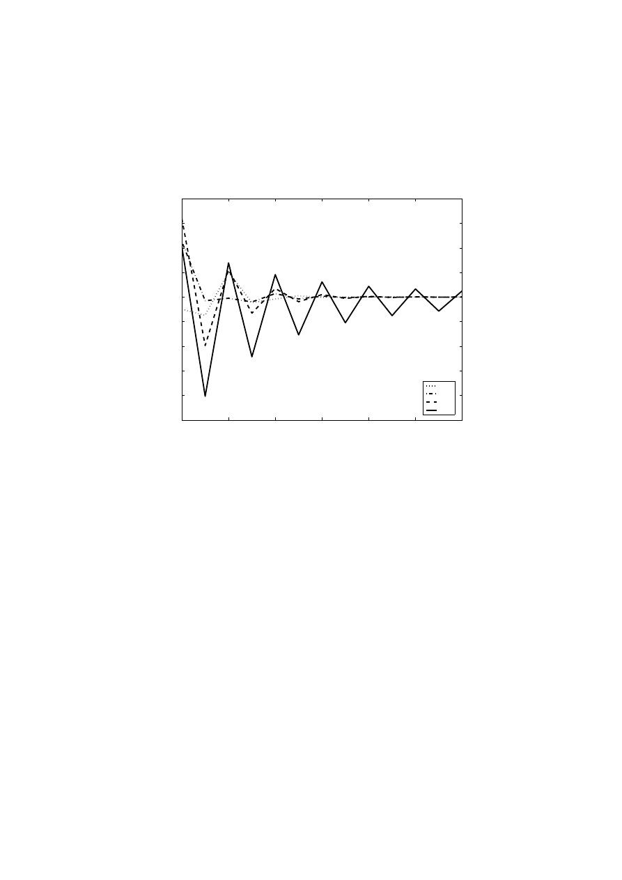
gence of this index is quite slow and oscillatory. Mutual information (Eq. 21)
converges faster, and the information gain ratio (Eq. 32) shows similar be-
havior as the Gini index (Eq. 39) and the symmetrical uncertainty coeﬃcient
J

(Eq. 35) that converge quickly, reaching correct values already for 8 bins

(Fig. 2). Good convergence and low bias make this coeﬃcient a very good
candidate for the best relevance index.

−0.1

−0.08

−0.06

−0.04

−0.02

0.02

0.04

0.06

0.08

Gini
J

MI
J

Fig. 2. Diﬀerences between the Gini, J

MI, and J

indices and their exact

value (vertical axis), as a function of the number of discretization bins (horizontal
axis).

8 Filters for feature selection

Relevance indices discussed in the previous sections treat each feature as in-
dependent (with the exception of Relief family of algorithms Sec. 3 and the
group correlation coeﬃcient Eq. 13), allowing for feature ranking. Those fea-
tures that have relevance index below some threshold are ﬁltered out as not
useful. Some feature selection algorithms may try to include interdependence
between features. Given a subset of features X and a new candidate feature
X with relevance index J(X) an index J({X, X}) for the whole extended set
is needed. In theory a rigorous Bayesian approach may be used to evaluate
the gain in accuracy of the Bayesian classiﬁer after adding a single feature.
For k features the rule is:

(X) =

,..x

max

P(y

, x

, . . . x

)

(42)

where the sum is replaced by integral for continuous features.

This formula converges slowly even in one dimension (Fig. 2), so the main

problem is how to reliably estimate the joint probabilities

P(y

, x

. . . x

The density of training data

∝ P(x)

goes rapidly to zero with the growing

dimensionality k of the feature space. Already for 10 binary features and less
than 100 data samples less than 10% of 2

bins are non-empty. Although vari-

ous histogram smoothing algorithms may regularize probabilities, and hashing
techniques may help to avoid high computational costs [15], reliable estima-
tion of A

(X) is possible only if the underlying distributions are fully known.

This may be useful as a “golden standard” to calculate error bounds, as it is
done for one-dimensional distributions, but it is not a practical method.

Calculating relevance indices for subsets selected from a large number of

features it is not possible to include full interactions between all the features.
Note however that most wrappers may evaluate full feature interactions, de-
pending on the classiﬁcation algorithm used. Approximations based on sum-
ming pair-wise interactions oﬀer a computationally less expensive alternative.
The CFS algorithm described in Sec. 3 is based on Eq. 13, calculating aver-
age correlation coeﬃcients between features and classes and between diﬀerent
features. Instead of a ratio for some relevance indices that may measure corre-
lation or dependency between features one may use a linear combination of the
two terms: J(Y, X; S) = J(Y, X) − β

s∈S

J(X, X

), where the user-deﬁned

constant β is introduced to balance the importance of the relevance J(Y, X)
and the redundancy estimated by the sum of feature-feature relevancies. Such
algorithm has been used with mutual information as the relevance measure by
Battiti [2]. In this way redundancy of features is (at least partially) taken into
account and search for good subsets of features may proceed at the ﬁlter level.
A variant of this method may use a maximum of the pair relevance J(X, X

)

instead of the sum over all features s ∈ S; in this case β is not needed and
fewer features will be recognized as redundant.

The idea of inconsistency or conﬂict – a situation in which two or more

vectors with the same subset of feature values are associated with diﬀerent
classes – leads to a search for subsets of features that are consistent [9]. This is
very similar to the indiscernability relations and the search for reducts in rough
set theory [45]. The inconsistency count is equal to the number of samples with
identical features, minus the number of such samples from class to which the
largest number of samples belong (thus if there is only one class the index is
zero). Summing over all inconsistency counts and dividing by the number of
samples m the inconsistency rate for a given subset is obtained. This rate is
an interesting measure of feature subset quality, for example it is monotonic
(in contrast to most other relevance indices), decreasing with the increasing
feature subsets. Features may be ranked according to their inconsistency rates,
but the main application of this index is in feature selection.

9 Summary and comparison

There are various restrictions on applications of the relevance indices discussed
in the previous sections. For example, some correlation coeﬃcients (such as the
χ

or Pearson’s linear correlation) require numerical features and cannot be

applied to features with nominal values. Most indices require probabilities that
are not so easy to estimate for continuous features, especially when the number
of samples is small. This is usually achieved using discretization methods [35].
Relevance indices based on decision trees may automatically provide such
discretization, other methods have to rely on external algorithms.

In Table 1 information about the most popular ﬁlters is collected, including

the formulas, the types of inputs X (binary, multivalued integer or symbolic,
or continuous values), and outputs Y (binary for 2-class, multivalued integer
for multiclass problems and continuous for regression).

The ﬁrst method, Bayesian accuracy A

, is based on observed probabil-

ities

P(y

, x

) and provides a “golden standard” for other methods. Relations

between the Bayesian accuracy and mutual information are known 31, and
such relations may be inferred for other information-based indices, but in
general theoretical results of this sort are diﬃcult to ﬁnd and many indices
are simply based on heuristics. New methods are almost never tested against
Bayesian accuracy for simple binary features and binary classes. Diﬀerences
in ranking of features between major relevance indices presented in Sec. 7
are probably ampliﬁed in more general situations, but this issue has not been
systematically investigated so far.

Other methods that belong to the ﬁrst group of methods in Tab. 1 are

somehow special. They are based on evaluation of confusion matrix elements
and thus are only indirectly dependent on probabilities

P(y

, x

). Confusion

matrix may be obtained by any classiﬁer, but using Bayesian approach for clas-
siﬁcation balanced accuracy, area-under-curve (AUC), F-measure, Bi-normal
separation and odds ratio are still the best possible approaches, assuming
speciﬁc costs of diﬀerent type of errors.

Many variants of a simple statistical index based on separation of the

class means exist. Although these indices are commonly applied to problems
with binary targets extension to multiple target values is straightforward. In
practice pair-wise evaluation (single target value against the rest) may work
better, ﬁnding features that are important for disrimination of small classes.
Feature values for statistical relevance indices must be numerical, but target
values may be symbolic. Pearson’s linear correlation coeﬃcient can be applied
only for numerical feature and target values, and its averaged (or maximum)
version is used for evaluation of correlations with a subset of features. Decision-
tree based indices are applicable also to symbolic values and may be computed
quite rapidly. Some trees may capture the importance of a feature for a local
subset of data handled by the tree nodes that lie several levels below the root.
The Relief family of methods are especially attractive because they may be

Met

mmen

sian

accu

racy

theo

reti

the

lden

sta

nda

rd,

rescaled

esian

relev

Balan

accu

racy

iﬁ

;

sam

for

rget

Bi-

orm

sep

arat

ion

sed

format

ion

ret

riev

F-

measu

recall

recision

lar

form

ion

ret

riev

Odds

lar

format

ion

ret

riev

Mean

sep

arat

ion

sed

class

ean

Fish

er’s

criterion

T-

ist

ics

arson

orrelat

ion

lin

ear

orrelat

ion

sign

iﬁ

ased

tat

ion

Grou

orrelat

ion

n’

ﬃc

subs

ture

resu

lts

samp

les

lief

family

met

form

for

simp

liﬁ

rsion

eliefX

cap

res

cal

orrelat

ion

feat

teract

ion

rab

ilit

lit

tre

inde

ogoro

ist

iferen

een

join

rob

ilit

ies

sian

asu

same

trop

Gin

llb

-Leib

ler

ergen

len

format

ion

Jeﬀ

rey

Mat

sit

ist

rarely

used

but

rth

try

ing

iﬀ

eren

Met

ric

sed

for

lic

similarit

-b

ased

met

lic

feat

re-

feat

orrelat

ion

form

ion

len

form

ion

gain

form

ion

ain

format

ion

gain

feat

trop

ion

ical

cert

ain

ias

for

alu

feat

res

J-

asu

res

form

ion

logical

igh

far

rarely

sed

ias

for

alu

feat

res

relev

asu

res

for

ﬁ

ers.

res

target

the

(+),

tiv

alu

(sy

olic)

(in

ger)

lic

imp

lies

teger)

con

tin

real

Met

ith

applied in all situations, have low bias, include interaction among features and
may capture local dependencies that other methods miss.

Continuous target values are especially diﬃcult to handle directly, but

distance-based measures of similarity between distributions may handle them
without problems. Kolmogorov distance and other relevance indices from this
group may be expressed either by a sum of discrete probabilities or an inte-
gral over probability density functions. Bayesian measure, identical with the
Gini index for discrete distributions, generalizes it to continuous features and
continuous targets. The only exception in this group is the Value Diﬀerence
Metric that has been speciﬁcally designed for symbolic data.

Indices based on information theory may also be used for continuous fea-

tures and targets if probability densities are deﬁned. Information gain ratio
and symmetrical uncertainty coeﬃcient are especially worth recommending,
sharing low bias with the MDL approach (Sec. 5), and converging in a stable
and quick way to their correct values.

10 Discussion and conclusions

Filters provide the cheapest approach to the evaluation of feature relevance.
For a very large number of features they are indispensable, and only after ﬁl-
tering out most of the features other, more expansive feature selection methods
become feasible.

Many approaches to ﬁlters discussed in the preceding sections show that

there is no simple answer to the question: which relevance index is the best
to construct a good ﬁlter? If there is suﬃcient data and joint probabilities
may be estimated in a reliable way there is no reason why Bayesian relevance
J

should not be used. After all other relevance indices, and in particular

indices based on the theory of information, are only approximations to the
Bayesian relevance. Unfortunately this index seems to be the most diﬃcult
to estimate reliably (see Fig. 2), leaving room for other approaches. In some
applications including costs of diﬀerent types of misclassiﬁcations (Sec. 2) is
a better choice of relevance index, leading to the balanced accuracy (Eq. 4),
F-measure or optimization of ROC curves. Evaluation of all such quantities
will suﬀer from the same problem as evaluation of the Bayesian relevance
J

, and therefore other, approximate but more reliable methods should be

studied.

Diﬀerent approaches to relevance evaluation lead to a large number of in-

dices for ranking and selection. Certainly more papers with new versions of
relevance indices for information ﬁlters will be published, but would they be
more useful? As noted in the book on CART [4] the splitting criteria do not
seem to have much inﬂuence on the quality of decision trees, so in the CART
tree an old index known as Bayesian measure J

(Eq. 19) or Vajda En-

tropy (Eq. 23) has been employed, under the new name “Gini”. Perhaps the

actual choice of feature relevance indices also has little inﬂuence on perfor-
mance of ﬁlters. For many applications a simple approach, for example using
a correlation coeﬃcient, may be suﬃcient.

Not all options have been explored so far and many open questions re-

main. Similarities, and perhaps equivalence up to monotonic transformation
of relevance indices, should be established. The reliability of estimation of
relevance indices – with the exception of entropy estimations – is not known.
Biases towards multi-valued features of several indices have been identiﬁed
but their inﬂuence on ranking is not yet clear. Little eﬀort has been devoted
so far towards cost-sensitive feature selection. In this respect the accuracy of
Bayesian classiﬁcation rules and other performance metrics related to logical
rules are worth investigating.

Not much attention has been paid towards speciﬁc class-oriented and lo-

cal, context-dependent ﬁlters. Some problems (especially in bioinformatics)
require the simultaneous identiﬁcation of several features that may individu-
ally have quite poor relevance. The paradigmatic benchmark problems of this
sort are the parity problems, starting from the XOR. Only context-dependent
local feature selection methods (like Relief, or ﬁlter methods applied to vectors
in a localized feature space region) seem to be able to deal with such cases. Al-
though our knowledge of ﬁlter-based feature selection has signiﬁcantly grown
in recent years still much remains to be done in this ﬁeld.

Acknowledgment: I am grateful to Jacek Biesiada for drawing my at-

tention to many papers in this ﬁeld, and to Norbert Jankowski and Krzysztof
Gr¸

abczewski for critically reading this paper.

References

1. A. Antos, L. Devroye, and L. Gyorﬁ. An extensive empirical study of feature

selection metrics for text classiﬁcation. IEEE Transactions on Pattern Analysis
and Machine Intelligence, 21(7):643–645, 1999.

2. R. Battiti. Using mutual information for selecting features in supervised neural

net learning. IEEE Trans. on Neural Networks, 5:537–550, 1991.

3. D.A. Bell and H. Wang. A formalism for relevance and its application in feature

subset selection. Machine Learning, 41:175–195, 2000.

4. L. Breiman, J.H. Friedman, R.A. Olshen, and C.J. Stone. Classiﬁcation and

Regression Trees. Wadsworth and Brooks, Monterey, CA, 1984.

5. L. Bruzzone, F. Roli, and S.B. Serpico. An extension of the jeﬀreys-matusita dis-

tance to multiclass cases for feature selection. IEEE Transactions on Geoscience
and Remote Sensing, 33(6):1318–1321, 1995.

6. F.M. Coetzee, E. Glover, L. Lawrence, and C.L Giles.

Feature selection in

web applications by roc inﬂections and powerset pruning. In Proceedings of
2001 Symp. on Applications and the Internet (SAINT 2001), pages 5–14, Los
Alamitos, CA, 2001. IEEE Computer Society.

7. T.M. Cover. The best two independent measurements are not the two best.

IEEE Transactions on Systems, Man, and Cybernetics, 4:116–117, 1974.

8. D.R. Cox and D.V. Hinkley. Theoretical Statistics. Chapman and Hall/CRC

Press, Berlin, Heidelberg, New York.

9. M. Dash and H. Liu. Consistency-based search in feature selection. Artiﬁcial

Intelligence, 151:155–176, 2003.

10. R.L. de Mantaras. A distance-based attribute selection measure for decision

tree induction. Machine Learning Journal, 6:81–92, 1991.

11. L. Devroye, L. Gyrﬁ, and G. Lugosi. A Probabilistic Theory of Pattern Recog-

nition. Springer, Berlin, Heidelberg, New York, 1996.

12. W. Duch, R. Adamczak, and K. Gr¸

abczewski. A new methodology of extraction,

optimization and application of crisp and fuzzy logical rules. IEEE Transactions
on Neural Networks, 12:277–306, 2001.

13. W. Duch and L. Itert. A posteriori corrections to classiﬁcation methods. In

L. Rutkowski and J. Kacprzyk, editors, Neural Networks and Soft Computing,
pages 406–411. Physica Verlag, Springer, Berlin, Heidelberg, New York, 2002.

14. W. Duch, R. Setiono, and J. Zurada. Computational intelligence methods for

understanding of data. Proceedings of the IEEE, 92(5):771–805, 2004.

15. W. Duch, T. Winiarski, J. Biesiada, and A. Kachel. Feature ranking, selection

and discretization. In Proceedings of Int. Conf. on Artiﬁcial Neural Networks
(ICANN), pages 251–254, Istanbul, 2003. Bogazici University Press.

16. R.O. Duda, P.E. Hart, and D.G. Stork. Patter Classiﬁcation. John Wiley &

Sons, New York, 2001.

17. D. Erdogmus and J.C. Principe. Lower and upper bounds for misclassiﬁcation

probability based on renyis information.

Journal of VLSI Signal Processing

Systems, 37(2-3):305–317, 2004.

18. G. Forman. An extensive empirical study of feature selection metrics for text

classiﬁcation. Journal of Machine Learning Research, 3:1289–1305, 2003.

19. E.E. Ghiselli. Theory of psychological measurement. McGrawHill, New York,

1964.

20. K. Gr¸

abczewski and W. Duch. The separability of split value criterion. In

Proceedings of the 5th Conf. on Neural Networks and Soft Computing, pages
201–208, Zakopane, Poland, 2000. Polish Neural Network Society.

21. M.A. Hall. Correlation-based Feature Subset Selection for Machine Learning.

PhD thesis, Department of Computer Science, University of Waikato, Waikato,
N.Z., 1999.

22. D.J. Hand. Construction and assessment of classiﬁcation rules. J. Wiley and

Sons, Chichester, 1997.

23. J.A. Hanley and B.J. McNeil. The meaning and use of the area under a receiver

operating characteristic (roc) curve. Radiology, 143:29–36, 1982.

24. R.M. Hogarth.

Methods for aggregating opinions.

In H. Jungermann and

G. de Zeeuw, editors, Decision Making and Change in Human Aﬀairs. D. Reidel
Publishing, Dordrecht, Holland, 1977.

25. D. Holste, I. Grosse, and H. Herzel. Bayes’ estimators of generalized entropies.

J. Physics A: Math. General, 31:2551–2566, 1998.

26. R.C. Holte. Very simple classiﬁcation rules perform well on most commonly

used datasets. Machine Learning, 11:63–91, 1993.

27. S.J. Hong. Use of contextual information for feature ranking and discretization.

IEEE Transactions on Knowledge and Data Engineering, 9:718–730, 1997.

28. Z. Ahmed M. Brown I Guyon, H-M Bitter and J. Heller. Multivariate non-linear

feature selection with kernel multiplicative updates and gram-schmidt relief. In
BISC FLINT-CIBI 2003 workshop, Berkeley, Dec. 2003, 2003.

29. G.V. Kass. An exploratory technique for investigating large quantities of cate-

gorical data. Applied Statistics, 29:119–127, 1980.

30. R. Kohavi and G. John. Wrappers for feature subset selection. Artiﬁcial Intel-

ligence, 97(1-2):273–324, 1996.

31. I. Kononenko. On biases in estimating the multivalued attributes. In Proceed-

ings of IJCAI-95, Montreal, pages 1034–1040, San Mateo, CA, 1995. Morgan
Kaufmann.

32. N. Kwak and C-H. Choi. Input feature selection by mutual information based

on parzen window. IEEE Transactions on Pattern Analysis and Machine Intel-
ligence, 24:1667–1671, 2002.

33. N. Kwak and C-H. Choi. Input feature selection for classiﬁcation problems.

IEEE Transactions on Neural Networks, 13:143–159, 2002.

34. M. Li and P. Vit´

anyi. An Introduction to Kolmogorov Complexity and Its Ap-

plications. Text and Monographs in Computer Science. Springer, Berlin, Hei-
delberg, New York, 1993.

35. H. Liu, F. Hussain, C.L. Tan, and M. Dash. Discretization: An enabling tech-

nique. Journal of Data Mining and Knowledge Discovery, 6(4):393–423, 2002.

36. H. Liu and R. Setiono. Feature selection and discretization. IEEE Transactions

on Knowledge and Data Engineering, 9:1–4, 1997.

37. D. Michie. Personal models of rationality. J. Statistical Planning and Inference,

21:381–399, 1990.

38. R. Moddemeijer. A statistic to estimate the variance of the histogram based

mutual information estimator based on dependent pairs of observations. Signal
Processing, 75:51–63, 1999.

39. A.Y. Ng.

On feature selection: learning with exponentially many irrelevant

features as training examples. In Proceedings of the 15th International Confer-
ence on Machine Learning, pages 404–412, San Francisco, CA, 1998. Morgan
Kaufmann.

40. W.H. Press, S.A. Teukolsky, W.T. Vetterling, and B.P. Flannery. Numerical

recipes in C. The art of scientiﬁc computing. Cambridge University Press, Cam-
bridge, UK, 1988.

41. J.R. Quinlan. C4.5: Programs for Machine Learning. Morgan Kaufman, San

Mateo, CA, 1993.

42. M. Robnik-Sikonja and I. Kononenko. Theoretical and empirical analysis of

relieﬀ and rrelieﬀ. Machine Learning, 53:23–69, 2003.

43. P. Smyth and R.M. Goodman. An information theoretic approach to rule induc-

tion from databases. IEEE Transactions on Knowledge and Data Engineering,
4:301–316, 1992.

44. J.A. Swets. Measuring the accuracy of diagnostic systems. Proceedings of the

IEEE, 240(5):1285–1293, 1988.

45. R.W. Swiniarski and A. Skowron. Rough set methods in feature selection and

recognition. Pattern Recognition Letters, 24:833–849, 2003.

46. K. Torkkola. Feature extraction by non parametric mutual information maxi-

mization. Journal of Machine Learning Research, 3:1415–1438, 2003.

47. G.T. Toussaint. Note on optimal selection of independent binary-valued features

for pattern recognition. IEEE Transactions on Information Theory, 17:618–618,
1971.

48. I. Vajda. Theory of statistical inference and information. Kluwer Academic

Press, London, 1979.

49. C.J. van Rijsbergen. Information Retrieval. Butterworths, London, 1979.
50. T.R. Vilmansen. Feature evaluation with measures of probabilistic dependence.

IEEE Transactions on Computers, 22:381–388, 1973.

51. D.R. Wilson and T.R. Martinez. Improved heterogeneous distance functions.

Journal of Artiﬁcial Intelligence Research, 6:1–34, 1997.

Wyszukiwarka

Podobne podstrony:
Niechaj zstąpi Duch Twój
Efficient VLSI architectures for the biorthogonal wavelet transform by filter bank and lifting sc
Applications of polyphase filters for bandpass sigma delta analog to digital conversion
Fine Filters CJC
Marynarski duch, ZHP - przydatne dokumenty, Zbiórki pojedyncze
bb5 chap3
EMI Suppression Filters EMIFIL Nieznany
Duch od stepu, Lektury Okresy literackie
Choloniecki Duch dziejów Polski
MOKOSZ - duch słowiański, MITOLOGIE ŚWIATA
j g ?llard duch walki
H P Lovecraft Duch ciemności
26 Duch?solutny u Hegla
3. Duch Święty, 3
FILTRY 3, //1) Simple comb filter
Konspekt oraz materiały uzupełniające, Duch człowieczy, Duch człowieczy
NOWY RÓŻANIEC DUCH BUGNINIEGO !!!

więcej podobnych podstron