
WP/14/
186
A Model-Based Analysis of Spillovers:
The Case of Poland and the Euro Area
Michal Andrle, Roberto Garcia-Saltos, and Giang Ho

© 2014 International Monetary Fund
WP/14/
186
IMF Working Paper
Research Department
A Model-Based Analysis of Spillovers:
The Case of Poland and the Euro Area
1
Prepared by Michal Andrle, Roberto Garcia-Saltos, and Giang Ho
Authorized for distribution by Benjamin Hunt
October 2014
Abstract
This paper studies economic and financial spillovers from the euro area to Poland in a
two-country semi-structural model. The model incorporates various channels of macro-
financial linkages and cross-border spillovers. We parameterize the model through an
extensive calibration process, and provide a wide range of model properties and
evaluation exercises. Simulation results suggest a prominent role of foreign demand
shocks (euro area and global) in driving Poland’s output, inflation and interest rate
dynamics, particularly in recent years. Our model also has the capability for medium-term
conditional forecasting and policy analysis.
JEL Classification Numbers:
Keywords: Poland, Euro area, semi-structural model, spillovers
Author’s E-Mail Address: mandrle@imf.org; rgarciasaltos@imf.org; gho@imf.org
1
We would like to thank Julie Kozack, Christian Ebeke and Ben Hunt for valuable comments and suggestions. All
responsibility for errors remains with the authors.
This Working Paper should not be reported as representing the views of the IMF.
The views expressed in this Working Paper are those of the author(s) and do not necessarily
represent those of the IMF or IMF policy. Working Papers describe research in progress by the
author(s) and are published to elicit comments and to further debate.

2
Contents
Page
I.
Introduction . . . . . . . . . . . . . . . . . . . . . . . . . . . . . . . . . . . . . .
II.
A Model of Poland and the Euro Area . . . . . . . . . . . . . . . . . . . . . . . .
A.
Modeling philosophy . . . . . . . . . . . . . . . . . . . . . . . . . . . . . . .
B.
Model structure
. . . . . . . . . . . . . . . . . . . . . . . . . . . . . . . . .
1.
Output . . . . . . . . . . . . . . . . . . . . . . . . . . . . . . . . . . . .
2.
Unemployment
. . . . . . . . . . . . . . . . . . . . . . . . . . . . . . .
3.
Inflation dynamics . . . . . . . . . . . . . . . . . . . . . . . . . . . . . .
4.
Exchange rate dynamics . . . . . . . . . . . . . . . . . . . . . . . . . . .
5.
Monetary policy . . . . . . . . . . . . . . . . . . . . . . . . . . . . . . .
6.
Euro area block . . . . . . . . . . . . . . . . . . . . . . . . . . . . . . .
C.
Linkages and spillovers . . . . . . . . . . . . . . . . . . . . . . . . . . . . .
D.
Data
. . . . . . . . . . . . . . . . . . . . . . . . . . . . . . . . . . . . . . .
III.
Model Parameterization . . . . . . . . . . . . . . . . . . . . . . . . . . . . . . . .
IV.
Model Properties & Evaluation . . . . . . . . . . . . . . . . . . . . . . . . . . . .
A.
Impulse response functions
. . . . . . . . . . . . . . . . . . . . . . . . . . .
B.
Correlation analysis . . . . . . . . . . . . . . . . . . . . . . . . . . . . . . .
C.
Variance decomposition . . . . . . . . . . . . . . . . . . . . . . . . . . . . .
D.
Policy analysis . . . . . . . . . . . . . . . . . . . . . . . . . . . . . . . . . .
E.
Estimates of trends and structural shocks . . . . . . . . . . . . . . . . . . . .
F.
Historical shock decomposition . . . . . . . . . . . . . . . . . . . . . . . . .
1.
Output . . . . . . . . . . . . . . . . . . . . . . . . . . . . . . . . . . . .
2.
Inflation . . . . . . . . . . . . . . . . . . . . . . . . . . . . . . . . . . .
G.
Recursive forecast and conditional forecasting . . . . . . . . . . . . . . . . .
V.
Concluding Remarks . . . . . . . . . . . . . . . . . . . . . . . . . . . . . . . . .
References . . . . . . . . . . . . . . . . . . . . . . . . . . . . . . . . . . . . . . . . . .
Appendices
A.
Model equations . . . . . . . . . . . . . . . . . . . . . . . . . . . . . . . . . . . .
B.
Tables and figures . . . . . . . . . . . . . . . . . . . . . . . . . . . . . . . . . . .
Tables
1.
Calibrated Dynamic Parameters . . . . . . . . . . . . . . . . . . . . . . . . . . . .
2.
Calibrated Stochastic Parameters . . . . . . . . . . . . . . . . . . . . . . . . . . .
Figures
1.
Stylized facts – trends . . . . . . . . . . . . . . . . . . . . . . . . . . . . . . . . .

3
2.
Stylized facts – cycle . . . . . . . . . . . . . . . . . . . . . . . . . . . . . . . . .
3.
Model-based “core” inflation versus trimmed mean inflation
. . . . . . . . . . . .
4.
Interbank market premium . . . . . . . . . . . . . . . . . . . . . . . . . . . . . .
5.
Shock to domestic demand (ε
y
,ar
t
) . . . . . . . . . . . . . . . . . . . . . . . . . . .
6.
Negative shock to foreign demand (ε
y
∗
,iid
t
) . . . . . . . . . . . . . . . . . . . . . .
7.
Negative global demand shock (ε
com
t
) . . . . . . . . . . . . . . . . . . . . . . . . .
8.
Shock to home core inflation (ε
π
core
t
) . . . . . . . . . . . . . . . . . . . . . . . . .
9.
Shock to domestic monetary policy (ε
I
t
) . . . . . . . . . . . . . . . . . . . . . . .
10.
Permanent disinflation shock (ε
π
tar
t
) . . . . . . . . . . . . . . . . . . . . . . . . . .
11.
Shock to exchange rate (ε
S
t
) . . . . . . . . . . . . . . . . . . . . . . . . . . . . . .
12.
Shock to foreign interbank market premium (ε
χ
∗
t
) . . . . . . . . . . . . . . . . . .
13.
Output gap, core inflation and interest rates – Correlations (2000Q1 - 2012Q4) . . .
14.
Forecast error variance decomposition for Poland and Euro area
. . . . . . . . . .
15.
Counterfactual 1: Responses to euro area demand shock with monetary policy delay
16.
Counterfactual 2: Responses to euro area financial shock with higher shock per-
sistence . . . . . . . . . . . . . . . . . . . . . . . . . . . . . . . . . . . . . . . .
17.
Estimated output gap, core inflation, and equilibrium variables . . . . . . . . . . .
18.
Historical shock decomposition - Output . . . . . . . . . . . . . . . . . . . . . . .
19.
Historical shock decomposition - Inflation . . . . . . . . . . . . . . . . . . . . . .
20.
Conditional in-sample forecast (8 quarters ahead) . . . . . . . . . . . . . . . . . .
21.
Non-core “wedge” and oil prices . . . . . . . . . . . . . . . . . . . . . . . . . . .

4
I. I
NTRODUCTION
The recent episodes of financial and sovereign stress in the euro area have rekindled concerns
over potential spillover effects to emerging Europe. This paper studies spillovers from the
euro area to Poland, specifically seeking to answer one question: to what extent developments
in the euro area drive Poland’s output, inflation, and interest rate dynamics. Poland makes a
nice case for studying this issue, being a small open economy with extensive trade and finan-
cial linkages with euro area countries. For example, in 2011 over half of Polish exports went
to euro area countries, and about sixty percent of the Polish banking system is owned by core
euro area banks. Business cycles in Poland and the euro area have also become increasingly
It is therefore crucial for policy making and forecasting to understand the im-
pact of international shocks on the economy and analyze their transmission mechanisms in an
internally and externally consistent framework.
We build a semi-structural, forward-looking, two-country model with emphasis on cyclical
dynamics of the economy. The model uses a small number of behavioral equations, derived
from economic theory (although not fully developed from micro foundations), to character-
ize the evolution of key macroeconomic variables, such as output, inflation, interest rate, and
the exchange rate. Linkages between Poland, modeled as a small open economy, and the euro
area work through both real and financial channels. We introduce cross-border links in the
interbank market premium to capture the early transmission of financial stress, especially in
periods of market turmoil, as observed at the start of the 2008-09 crisis. Model parameteriza-
tion is based on an extensive calibration process, and we provide an evaluation of the model’s
properties. Our model allows for identification of key structural shocks, notably country-
specific and common (or global) demand shocks. The model is suited for medium-term fore-
casting and for constructing counterfactuals for policy analysis.
Our results suggests that Poland’s economy has become more susceptible to external shocks.
For example, foreign shocks (of either euro area or global origin) on average account for a lit-
tle over half of Poland’s output volatility, and about a quarter of its inflation cyclical dynam-
ics. Poland’s exchange rate flexibility has played a key stabilizing role. The results using the
semi-structural model are consistent with evidence from a VAR model analysis of the Polish
economy in
The paper is organized as follows. In Section
we describe the model structure. In Section
we discusses model parameterization. Selected results from model simulation are pre-
1
For example, the simple correlation in quarterly year-on-year growth rates for the post-2004 period is 0.81.

5
sented in Section
, and in Section
we conclude with the main take-aways from our analy-
sis.
II. A M
ODEL OF
P
OLAND AND THE
E
URO
A
REA
A. Modeling philosophy
The model is built and designed top-down, with an eye on its aggregate properties, while also
being informed by observed data. We impose much of the discipline brought by structural
dynamic stochastic general equilibrium models (DSGE) but relax their strict assumptions
when deemed useful.
The model is trend-cyclical, i.e. it focuses on business cycle dynamics of the data in a struc-
tured way. Trends are characterized by a system of interlinked stochastic processes, which
have economic interpretation but are not based upon explicit optimizing behavior. Modelling
Poland’s trend developments in a fully structural way is beyond the scope of this paper and
would require elements such as the process of income convergence, technology adoption and
foreign direct investment, trend real exchange rate appreciation due to the Balassa-Samuelson
effect, and variation in the inflation target during the process of disinflation, and others. Fur-
ther, the differential growth rates between the euro area and Poland or the increase in trade
openness (as manifested by increasing export shares in GDP) would require modeling off-
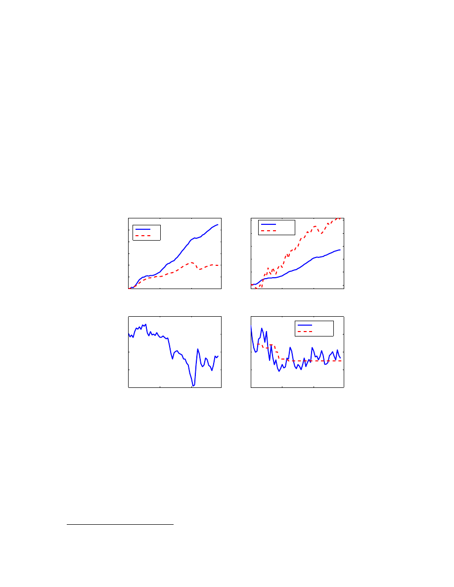
balanced growth convergence in a complex way, as suggested by the stylized facts in Figure
We proceed, however, with the assumption that productivity growth shocks drive primarily
the low frequencies of the data. The cyclical dynamics due to these productivity shocks then
may resemble a demand shock, when the wealth effect results in an increase in output and lit-
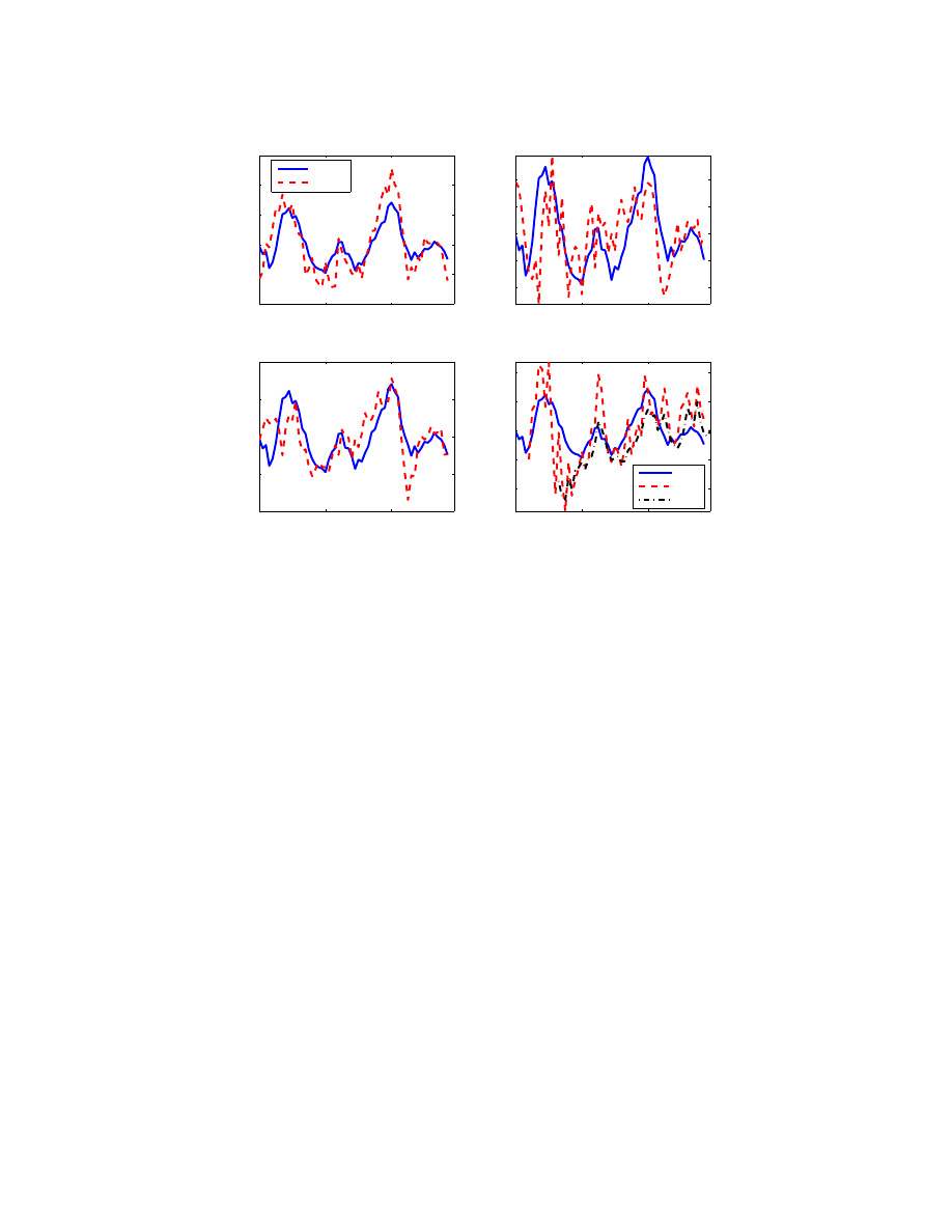
tle change or a small increase in inflation. The cyclical dynamics of the Polish economy seem
consistent with the dominance of demand shocks, as exemplified by the positive comovement
of the cyclical component of output and the deviation of inflation from the inflation target
(Figure
Our model fits into a family of the existing models of the Polish economy. On one hand, there
is the National Bank of Poland (NBP)’s projection model NECMOD (see, for instance,
) or
)), a large-scale econometric model with
6
ad-hoc short-run dynamics, with a relatively limited role for active interest rate policy.
And
on the other hand, NBP developed a complex, estimated DSGE model SOE-PL (see, for in-
stance,
)), a medium-size model derived from ‘micro foun-
dations,’ featuring a full stock-flow consistency. Our model fits in between these two type
of models. Compared to SOE-PL, it is a less restricted and less rigorous smaller version of a
structural DSGE model, though with a more elaborate version of the foreign block. It shares
its focus on cyclical dynamics but the dynamics of trends are modeled jointly with the cycli-
cal dynamics. With respect to NECMOD, our model is more aggregated and relies more on
forward-looking dynamics of policy rate and the inflation targeting regime.
Figure 1. Stylized facts – trends
1998:1
2003:1
2008:1
0
10
20
30
40
50
60
Output (100*log)
PL
EU
1998:1
2003:1
2008:1
0
20
40
60
80
100
Output and Exports (100*log)
output
exports
1998:1
2003:1
2008:1
−60
−40
−20
0
20
Real exchange rate (100*log)
1998:1
2003:1
2008:1
−5
0
5
10
15
Inflation (% q/q ann.)
headline
target
B. Model structure
The model is essentially a one sector, small open economy, New Keynesian model. The real
interest rate affects households and firms via intertemporal decisions, forward-looking mon-
etary policy determines the nominal rate of interest, and nominal rigidities are formalized
2
By ad hoc we intend its literal meaning ‘for this,’ meaning a solution created for a specific problem.
7
Figure 2. Stylized facts – cycle
1998:1
2003:1
2008:1
−4
−2
0
2
4
6
Domestic Demand
output
demand
1998:1
2003:1
2008:1
−2
−1
0
1
2
Exports
1998:1
2003:1
2008:1
−4
−2
0
2
4
Imports
1998:1
2003:1
2008:1
−4
−2
0
2
4
Inflation −− headline and trimmed mean (% q/q ann.)
output
CPI
TRIMM
Note: Band pass cycles, scaled to output variance in percent. In each subplot, the solid blue line represents output.
using a version of a New Keynesian Phillips curve. The exchange rate ties the domestic and
foreign interest rate according to a version of uncovered interest rate parity (UIP). The list of
relevant behavioral equations is included in Appendix
Notation and units of the model: We use the symbol ∗ to distinguish euro area variables
from domestic (Poland) variables, uppercase letters to denote the variables themselves, ¯
X
to
denote the trend or equilibrium value of variable X , and lowercase letters to denote deviations
from the time-varying trend (so that x = X − ¯
X
). Output and real exchange rate deviations are
in percent (100×log deviations). Nominal and real interest rates, inflation, unemployment,
and the rate of exchange rate depreciation are in percent per annum or annualized, respec-
tively. The frequency of the model is quarterly.
1. Output
Output is determined by the trend and cyclical component. Both the trend, or potential, output
and the cyclical component, or output gap, are modeled jointly and aggregate to total output:
Y
t
= ¯
Y
t
+ y
t
.
(1)

8
The domestic output gap, y
t
, is determined by the real interest rate, real exchange rate, and
foreign output. The factors behind output dynamics reflect key drivers of consumption, in-
vestment, and the trade balance. The expectational dynamics allow for both persistent effects
of past shocks and the expected path of real interest rate, real exhange rate, or foreign demand
to determine the current output growth:
y
t
= β
1
y
t
−1
+ β
2
y
t
+1
− β
3
[r
t
+ ˆ
χ
t
] + β
4
z
t
+ β
5
y
∗
t
+ ε
y
,iid
t
+ ε
y
,ar
t
+ ε
c f
t
.
(2)
The real interest rate and the real exchange rate affect both output and inflation and capture
the monetary policy of the central bank. It is the real interest rate deviation from its trend rate
r
t
= R
t
− ¯
R
t
, that is relevant for decisions of households and firms. The real interest rate is
defined using the Fisher relationship R
t
= I
t
− π
t
+1|t
, where I
t
denotes the nominal rate of
interest. Analogously, it is the real exchange rate deviation from its trend, z
t
, that is relevant
for the business cycle dynamics and inflation.
We acknowledge that the real interest rate relevant for households and firms may differ from
the risk-free policy rates. We augment the risk-free rate with an exogenous interest rate pre-
mium, ˆ
χ . We use the observed difference between the policy rate and the interbank lending
rate (WIBOR in Poland) to define the premium resulting from the increased counter-party
risk at interbank markets, as observed during the Great Recession. In reality, borrowers also
face an external finance premium—see for instance
) for descrip-
tion of financial accelerator mechanism—which evolves in a countercyclical manner as il-
lustrated also during the recent global financial crisis. We reflect the accelerator mechanism
directly in our calibration of semi-structural parameters and as a part of the shock to demand
ε
ar
t
Finally, there are two different types of demand shocks in the model. The first is a domestic
demand shock, ε
ar
t
, whereas the second is a common (global) demand shock to both Poland
and the euro area, ε
c f
t
. The effects of those two shocks are different, since the latter impacts
both economies and thus contributes to a global increase in resource utilization and demand
pressures. Whether there is a truly global demand shock is an interesting question. The litera-
ture on common world and regional cycles, for example
) or
), suggests there are strong commonalities across countries, but the analysis is a
3
Consider the simplest case of the external finance premium deviation from trend, say x f p
t
= κy
t
+ ε
x f p
t
, where
the premium responds to output cycle. By substituting such a premium into
, the output gap equation remains
unchanged, but the semi-structural parameters change, i.e. the coefficient on the real interest rate would increase.
That is a spirit of a financial accelerator. The shock to the premium would not be distinguishable from a demand
shock. More complex formulations are possible but for parsimony principles we opt out from using the external
finance premium formulation.

9
reduced-form one. The common shock, due to its distinct impulse response function, is iden-
tified and picks up the comovement unexplained by other factors and spillovers. The demand
shock ε
ar
t
is autocorrelated with persistence ρ
ar
, the common demand shock persistence is
ρ
c f
.
Having specified the cyclical component of output, the determination output is completed
by specifying the trend, or potential, level of output. Our specification follows
) and defines the trend output using a version of a local linear trend model.
Trend output is subject to level and growth rate shocks, with a well-defined steady-state out-
put growth that it converges towards:
Y
t
=
¯
Y
t
+ y
t
(3)
¯
Y
t
=
¯
Y
t
−1
+ µ
t
/4 + ε
¯
Y
t
(4)
µ
t
= ρ
µ
µ
t
−1
+ (1 − ρ
µ
)µ
ss
+ ε
µ
t
.
(5)
For simplification, we postulate a complete trend-cycle dichotomy between the output’s trend
and cycle components. In reality, there are likely to be permanent productivity shocks hitting
the Polish economy, which induce cyclical dynamics and wealth effects associated with ex-
pected long-run gains in productivity (for instance foreign direct investment and technology
adoption). Part of those shocks will be picked up in our demand shocks.
2. Unemployment
The specification of unemployment follows a dynamic version of Okun’s law. Unemploy-
ment’s cyclical dynamics make use of a robust empirical regularity in the relationship be-
tween unemployment and output, or Okun’s law:
u
t
= α
1
u
t
−1
+ (1 − α
1
)α
2
y
t
+ ε
u
t
.
(6)
The unemployment gap u
t
is a function of its lagged value, the contemporaneous output gap,
and a disturbance term ε
u
t
. Although unemployment does not interact with the rest of the
model in important ways, this equation allows us to exploit observed unemployment data.
Okun’s law is used only to back out the likely path of unemployment, given other variables,
and does not contribute to identification of structural shocks in our framework.

10
3. Inflation dynamics
Inflation dynamics are modeled in two steps, with headline and core inflation rates being de-
fined. Core, or underlying, inflation is driven by the New Keynesian Phillips curve that ties
current inflation to expected inflation and shocks that hit the economy. Domestic demand
pressures are represented by the output gap, y
t
, while the real exchange rate gap, z
t
, reflects
the exchange rate pass-through on inflation. Headline inflation combines core inflation and
direct effects of oil prices:
π
core
t
= λ
1
π
core
t
+1
+ (1 − λ
1
)π
core
t
−1
+ λ
2
y
t
+ λ
3
z
t
+ λ
4
lr poil
t
+ ε
π
core
t
, and
(7)
π
t
= (1 − ω)π
core
t
+ ωπ
oil
t
+ ε
π
t
.
(8)
The homogeneity of the inflation process, as indicated by the weights on lead and lagged in-
flation summing to one, is a crucial property of the model. There is nothing in
that pins
down the steady-state level of inflation. The long-run level of inflation is uniquely determined
by the decision of a monetary policy authority. The coefficients λ
2,3,4
play a complex role
determining jointly the weight of each inflation driver in the real marginal costs and their
speed of pass-through. In a fully structural model, the coefficient λ
1
would be determined by
the discount factor and the degree of indexation to past inflation or inflation target for firms
that do not re-optimize their prices in the current period, see
), and the value of λ
1
would be smaller than 1/2. The semi-structural nature
of the model respects the homogeneity, but does not restrict the coefficient in absolute terms.
The degree of nominal rigidity is determined largely by the slope of the Phillips curve.
Core inflation is unobservable in our model, that is we do not use observed data on core in-
flation. Our definition of core inflation differs from the often-used concept of CPI excluding
food and energy components. While we exclude the direct impacts of oil on core inflation,
the gradual pass-through of oil prices into other price categories is captured via a deviation
of the real price of oil from its trend, lr poil, in
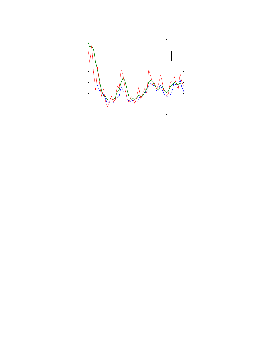
. Core inflation identified by our model is
close to a trimmed mean measure of inflation, as seen in Figure
, without the model using
the trimmed-mean inflation data.
4
National Bank of Poland (NBP) provides multiple measures of “core inflation”, including the 15% trimmed
mean measure.
See http://www.nbp.pl/homen.aspx?f=/en/statystyka/core.html
11
Figure 3. Model-based “core” inflation versus trimmed mean inflation
2000:1
2002:1
2004:1
2006:1
2008:1
2010:1
2012:1
−2
0
2
4
6
8
10
12
trimmed mean
model
headline inflation
Note: Q/Q annualized growth rates, seasonally adjusted
The model structure captures both the short-run and medium-term propagation of oil prices in
both economies. The gradual pass-through of oil prices via the real oil price gap is key to po-
tential second-round effects of oil prices and the reaction of monetary policy to those effects.
On the other hand, the immediate impact of oil prices on headline inflation via energy inten-
sive final goods, transportation, and fuels is hard for monetary policy to counter, but has only
a short-lived impact. The real price of oil follows an exogenous process and also responds to
the global output cycle.
There is a clear distinction between the effects of two cost-push shocks in the model. The
cost-push shock ε
core
t
is a long-lived cost-push shock. It is a supply-side shock, which propa-
gates through the economy for several quarters with a negative impact on aggregate demand
due to the reaction of the monetary policy authority. However, quarter-on-quarter dynam-
ics of inflation contain a great deal of non-persistent, high-frequency volatility, which often
can be explained by spikes in oil prices and exchange rate. Other times this volatility is un-
explainable by fundamentals. Joint modeling of a short-lived cost-push shock, ε
π
t
, with the
long-lived one allows the short-lived shock to pick-up the high-frequency volatility in cases
when fundamentals do not. The shock also works as a time-varying weight in the log-linear
identity

12
4. Exchange rate dynamics
An important part of international comovement is due to interconnected financial markets
and international arbitrage among many types of assets. In the model, financial arbitrage is
operationalized by a modified version of the uncovered interest parity (UIP):
I
t
= I
∗
t
+ 4 × (S
e
t
+1
− S
t
) + FX PREM
t
+ ε
S
t
(9)
¯
R
=
¯
R
∗
t
+ g
Z
,t
+ FX PREM
t
.
(10)
Equation
is uncovered interest parity (UIP), and equation
is a long-run version of UIP
which connects the trend component of real interest rates and trend real exchange rate depre-
ciation. This dual specification guarantees economic consistency among trends in the model,
and makes only the cyclical dynamics of interest rates and exchange rate subject to the arbi-
trage condition. While the UIP hypothesis is sometimes considered empirically implausible,
) investigates the hypothesis and finds evidence of the relationship between real
exchange rates and real interest rate differential at both trend and business cycle frequencies.
The exchange rate expectations, S
e
t
+1|t
, can deviate from pure model-consistent expectations,
S
t
+1|t
. Our specification follows
) and postulates that the expectation
is a weighted average of model-consistent expectations and the past level of the exchange rate
(taking into account the trend real appreciation), specifically:
S
e
t
+1|t
= δ S
t
+1|t
+ (1 − δ ) [S
t
−1
+ 2 × (g
Z
,t
− π
∗
ss
+ π
tar
,t
)/4] .
(11)
5. Monetary policy
The monetary policy authority sets the nominal rate of interest and determines the inflation
target. The policy interest rate (I
t
) is determined by an inflation-forecast-targeting interest rate
rule:
I
t
= (1 − γ
1
)[( ¯
R
t
+ π
tar
t
+1
) + γ
2
(π
yoy
t
+4
− π
tar
t
+4
) + γ
3
y
t
] + γ
1
I
t
−1
+ ε
I
t
(12)
The central bank aims to achieve a policy rate on average that is the sum of the equilibrium
real interest rate and the announced inflation target ( ¯
R
t
+ π
tar
t
+1
), while adjusting the rate in re-
sponse to deviations of the expected year-on-year inflation rate from the target (π
yoy
t
+4
− π
tar
t
+4
)
and to the current output gap. In so doing, the central bank also attempts to smooth out move-
ments in the policy rate (lagged term).

13
The inflation target is public knowledge and assumed to be fully credible. On purpose, the
model does not explicitly account for issues related to imperfect credibility of the inflation
target or actions of the monetary policy authority. The inflation target is operationalized using
an exogenous process:
π
tar
t
= π
tar
t
−1
+ ε
π
tar
t
,
(13)
hence the changes in the target are perceived as permanent. In the case when an anticipated
time-varying path is announced in advance, the information set of agents can be augmented to
cover the whole path in all of our modeling exercises and use.
6. Euro area block
The euro area block follows a New Keynesian model of a closed economy. The euro area
economy is assumed to not be affected by economic developments in Poland given the rel-
ative size of the two economies. The cyclical dynamics of the EA model are determined by:
y
∗
t
= β
∗
1
y
∗
t
−1
+ β
∗
2
y
∗
t
+1
− β
∗
3
[r
∗
t
+ ˆ
χ
∗
t
] + ε
y
∗
,iid
t
+ ε
y
∗
,ar
t
+ ε
com
t
(14)
π
∗
t
= (1 − ω
∗
)π
core
∗
t
+ ω
∗
π
oil
∗
t
+ ε
π
∗
t
(15)
π
core
∗
t
= λ
∗
1
π
core
∗
t
+1
+ (1 − λ
∗
1
)π
core
∗
t
−1
+ λ
∗
2
y
∗
t
+ λ
∗
4
lr poil
t
+ ε
π
core∗
t
(16)
I
∗
t
= (1 − γ
∗
1
)[ ¯
R
t
∗
+ π
tar
∗
t
+1
+ γ
∗
2
(π
yoy
∗
t
+4
− π
tar
∗
t
+4
) + γ
∗
3
y
∗
t
] + γ
∗
1
I
∗
t
−1
+ ε
I
∗
t
(17)
C. Linkages and spillovers
Our model incorporates the traditional macro-financial linkages, that is the interest rate, ex-
change rate, and trade channels. These traditional channels explain well the majority of his-
torical recessions that were precipitated by central banks tightening the policy rates in re-
sponse to demand pressures. Traditional channels should not be underestimated, as they form
a powerful source of international shock transmission. However, the more recent crises, in
particular the 2008-09 global financial crisis, were caused by shocks that were primarily fi-
nancial in nature. Financial developments (including asset price movements) played a precip-
itating role and served as a mechanism of propagating the crisis across markets and across
countries. Although the arbitrage principle embodied in uncovered interest parity ensures
close links between the euro area and Polish interest rates, macro-financial linkages can be
strengthened.
14
The changing nature of business cycles and cross-border linkages makes it necessary to find
ways to introduce into macro models other types of macro-financial linkages, over and be-
yond the standard interest rate and exchange rate effects.
We attempt to do it via the inter-
bank market premium and a global demand shock. Our measure of the interbank market pre-
mium is the spread between an interbank lending rate (3-month WIBOR for Poland, 3-month
EURIBOR for euro area) and the policy interest rate. This spread is close to zero in normal
times, but a rising spread can be an indicator of funding pressures in the interbank market
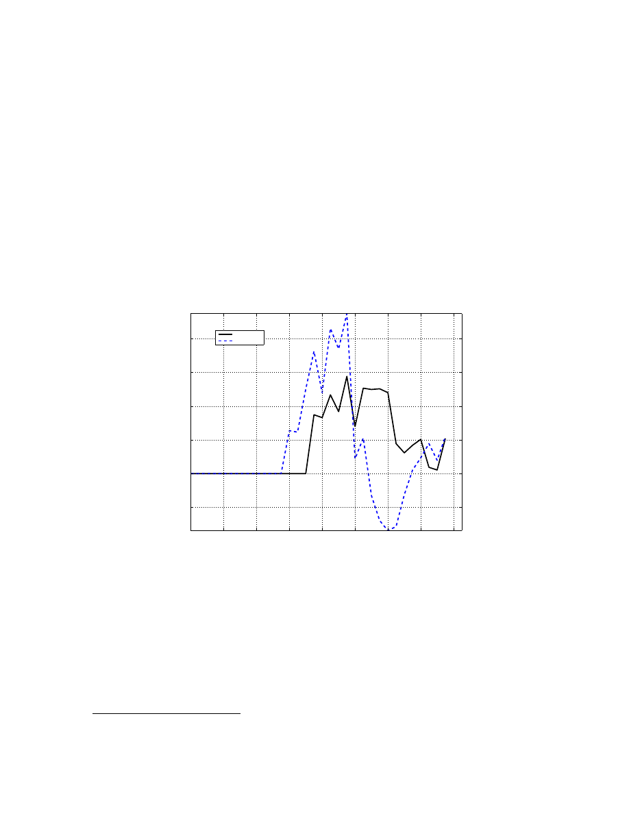
during a crisis. Figure
shows that at the peak of the 2008-09 crisis, when Lehman collapsed
in 2008Q3, the EURIBOR premium reached over 90bps, and the WIBOR premium almost
Figure 4. Interbank market premium
2004:1
2005:1
2006:1
2007:1
2008:1
2009:1
2010:1
2011:1
2012:1
−0.2
0
0.2
0.4
0.6
0.8
Poland (%)
Euro area (%)
We model the interbank market premiums as exogenous processes, with cross-country spill-
overs:
χ
t
= ρ
χ
χ
t
−1
+ (1 − ρ
χ
)[χ
SS
+ ψ(χ
∗
t
− χ
∗
SS
)] + ε
χ
t
, and
(18)
χ
∗
t
= ρ
χ
∗
χ
∗
t
−1
+ (1 − ρ
χ
∗
)χ
∗
SS
+ ε
χ
∗
t
.
(19)
We treat the premiums as exogenous, since they tend to be fast-moving financial indicators
triggered by liquidity problems in the interbank market. Therefore, they are largely indepen-
dent of the real economy. The parameter ψ governs the strength with which strains in the euro
5
See, for instance,
) for a discussion.
6
We set the pre-crisis premium, which were sufficiently close to zero, to exactly zero.

15
area’s interbank market are transmitted to the Polish interbank market, and captures the high
correlation of premium observed in the data.
The magnitude of spillovers also depends crit-
ically on the degree of persistence in the premium process (ρ
χ
∗
), that is how long agents ex-
pect financial markets in the euro area to remain unsettled. High premiums negatively affect
real output, as specified in equations
and
, potentially through a squeeze of credit sup-
ply as a result of liquidity dry-up in the interbank market. An advantage of this variable is
that it is available in a timely manner, possibly well in advance of output developments, and
therefore could be fed into the forecast, particularly in unusual episodes. The disadvantage is
that, by narrowly focusing on the first signs of trouble in financial markets that are not picked
up by normal interest rate movements, its potential impact on real economic activity can be
limited.
Our model also incorporates a common demand shock. The stylized shock is motivated by
empirical findings that common or global shocks, as opposed to country-specific shocks, are
the prominent source explaining international business cycle synchronization (see for instance
work by
)). The persistence of the common de-
mand shock is set identical to the persistence of the euro area demand shock, so the effect of
both is the same in the euro area. The identification of a common demand shock is thus deter-
mined by the reaction of the Polish economy. It turns out that the important aspect of the data
that identifies the common shock is the reaction of the real exchange rate.
D. Data
We use six observable variables for Poland, four for the euro area, and oil prices. The vari-
ables used for Poland’s economy are: real GDP, CPI inflation, the short-term nominal interest
rate, the interbank premium, the nominal exchange rate, and the inflation target. For the euro
area’s economy the variables are output, headline CPI inflation, policy rate, and the interbank
market premium.
The oil price is BRENT. Data are quarterly, and the sample spans 1999Q1-
2012Q2.
) provide a micro-founded theory for the international transmission of
financial shocks by incorporating a “global bank” into a two-country business cycle model.
8
We use the output gap estimate from the Global Projection Model with six regions, see e.g.

16
III. M
ODEL
P
ARAMETERIZATION
We choose to calibrate the parameters of the model. Bayesian estimation was considered, but
did not give robust results given the short sample (1999Q1 – 2012Q2) and questionable data
quality. In our modeling strategy we do not aim to build a model as a true data-generating
process. Instead, we see it as an eclectic approach to deal with policy analysis a forecasting.
Calibration allows us to blend data evidence, empirical results from other studies, and our
prior judgements on the model’s behavior in a flexible way.
Our parameterization aims to balance the story-telling power of the model with good multiple-
step ahead projection properties, coherence of model’s first and second moments with the
data, and economic plausibility of impulse response functions. In principle, we make use of
so-called ‘system priors’ (see
)) in our calibration process. System
priors seek to guide the estimates of model’s parameters that are consistent with a priori ag-
gregate properties of the model. For example, a demand shock is restricted to deliver a pos-
itive response of inflation and interest rates, with inflation returning to the target in no more
than three years. Another example is the prior about the sacrifice ratio – the cumulative out-
put loss after a permanent disinflation, which requires knowledge about the recent state of the
economy, the degree of monetary policy transparency, and nominal rigidities, etc. In general,
system priors impose discipline on a combination of dynamic parameters to ensure the model
generates sensible key properties, where sensibility is judged by both economic theory and
empirical evidence. This is especially important when the model is used in forecasting mode,
i.e., when it becomes part of the data generating process.
There are three groups of parameters. We distinguish coefficients affecting the steady-state,
the dynamics, and the stochastic processes. The steady-state values are set to reflect longer-
term tendencies of the variables and economic theory. Dynamic parameters are determined by
in-depth analysis of impulse-response behavior of the model, and–after stochastic parameters
are set–their estimates are finalized. The calibrated values for selected parameters are listed in
Tables
and
in Appendix
The values of steady-state coefficients reflect the trend development of both economies. Note
that the flexible local linear trend specification of trend output, the real exchange rate, etc. al-
lows for persistent deviation of the trend rate of change from the constant, steady-state growth
9
It is well known in the literature that maximum likelihood is the best choice in the case of the true model.
Slight misspecification, however, can have disastrous consequences. In our case, the maximum likelihood equiv-
alence to one-step-ahead forecast error minimization is also inconsistent with our emphasis on multi-step predic-
tion capabilities of the model, see e.g.

17
and real exchange rate appreciation. It is our prior that trends should be relatively smoother
than the actual path of variables, representing mostly low-frequency dynamics of model’s
We set the steady-state growth of the Polish economy to 3.5%, annualized, and
2% for the euro area. Steady-state inflation in Poland is 2.5%, in line with NBP’s official in-
flation target, and 1.9% in the euro area. We set the inflation target process as a random-walk
and respect the path and announcement of all changes in the inflation target since 1998, us-
ing the mean of the tolerance band. The trend real interest rate is 2.5% in the steady-state in
Poland and 2% in the euro area. Finally, the steady-state real exchange rate appreciation is
3.5% per year, consistent with the data. The steady-state levels of interbank premiums are
zero.
As mentioned above, an important concept is the sacrifice ratio. The baseline calibration,
in the case of perfectly credible monetary policy, implies the sacrifice ratio in Poland to be
roughly 0.4%, smaller than one would expect in the euro area. This is one of the most sen-
sitive statistics to parameterization, a concept that is only weakly identified by the data on a
particular country. The calibration reflects the recent state of the economy, a transparent mon-
etary policy, and the relatively smaller degree of nominal price and wage rigidities than in the
euro area, see
). Other important parameters include the
forward-looking coefficient of the Phillips curve, λ
1
= 0.45. The central bank’s interest rate
rule features a significant degree of inertia, γ
1
= 0.75, with a strict adherence to inflation tar-
geting with the weight on projected deviation from the target, λ
2
= 1.75, and on the output
gap, γ
3
= 0.25.
The role of oil prices is limited in our baseline calibration. That is not to say that oil prices
are not important for developments in the euro area and in Poland. The weight on oil –both
via direct and indirect effects– is calibrated to be larger in the euro area than in Poland. In
Poland, the direct effect was set close to zero, for parsimony, and the indirect, gradual effect
is λ
4
= 0.001. One reason is the role of administrated prices and energy regulation.
Further,
our model focuses on underlying inflation pressures, with our concept of unobserved core
inflation close to a trimmed mean measure of inflation, rather than headline excluding food
and energy. In essence, our measure works as a lower envelope of all core inflation measures
in Poland since 2003, see e.g. (
, pp. 26, Fig. 2.4).
10
Unless a priori restrictions are imposed on the estimation, or with misspecified models, the trend component
estimates may turn out rather volatile due to a ‘pile-up’ problem, see
). Theory implies
that the natural rate of output or natural rate of interest rate can be very volatile, as implied by the New Keynes-
ian models.
11
We find that in Poland oil prices (in national currency) hardly explain the wedge between headline inflation
and inflation excluding food and energies, while in the euro area the alignment is much stronger (Figure

18
Stochastic parameters were set to further advance the consistency of the model with the co-
variance structure of the data, and our priors about the structural interpretation of past data
by the model. Unlike the impulse-response functions, the population correlations and spec-
tral density of model variables are functions of all parameters, and offer testable implications.
Additional restrictions were based on the plausibility of the structural shock interpretation
of past developments, reflecting the narrative evidence and other studies, such as
Brzezina, Makarski, and Wesolowski
). In particular, our calibration of the relative stan-
dard deviation of domestic, euro area and common demand shocks also reflect findings from
VAR analyses of the roles of domestic and external shocks in Poland’s economy (see a com-
panion paper
IV. M
ODEL
P
ROPERTIES
& E
VALUATION
This section provides a discussion of model properties along many dimensions and examines
the spillovers between the euro area and Poland. Specifically, we present selected impulse-
response functions of the model, forecast-error variance decompositions, and population
cross-correlations of the model. Using the actual data, we interpret the economic develop-
ments in Poland using historical shock-decomposition analysis, and provide a conditional
recursive forecasting exercise to assess the forecasting properties of the model.
A. Impulse response functions
We present a selected set of impulse response functions (IRFs) from model simulations (Figures
to
). All shocks are of one standard deviation in their magnitude.
A demand shock in Poland (Figure
) puts pressure on core and headline inflation, triggering
a hike in the policy interest rate and real exchange rate appreciation. Foreign variables re-
main unchanged due to the small-open-economy assumption. The peak response of inflation
is roughly one third of the peak response of output. The inflation response is limited, as some
increase in demand can be satisfied from abroad. The monetary policy authority manoeuvres
the interest rate in such a way as to guide the inflation back to the target, which takes about
two and a half years.
Figures
and
show the responses to a negative demand shock from the euro area versus the
common world shock, respectively. A 1.5 percentage point drop in euro area’s output gap re-

19
duces home output gap by about 0.5 percentage point, dampening inflationary pressures, de-
creasing the policy interest rate and causing the real exchange rate to depreciate (which miti-
gates the negative effect on output). While similar, the responses are amplified in the case of
a common shock, since Poland would be affected not only directly but also indirectly through
weakening demand in the euro area. As a result, there is a larger drop in headline and core
inflation, a larger reduction in the policy interest rate, and a stronger depreciation of the ex-
change rate. In fact, it is the differential effect on Poland’s observed exchange rate that helps
identify a common shock from a euro area demand shock.
A shock to home core inflation, or a cost-push shock (Figure
), triggers reaction by the cen-
tral bank to increase the policy rate. Output falls in response to the real exchange rate appre-
ciation and expected increase in the real rates to curb the inflationary shock. Thus, unlike a
demand shock, a cost-push shock moves output and inflation in opposite directions. This is a
key identifying restriction the model uses when interpreting the available data evidence. Note
that the cost-push shock in our model has a negative effect on output solely due to a monetary
policy tightening. A monetary policy shock (Figure
) reduces inflation as well as output.
The effects of permanent disinflation can be studied with a permanent shock to the inflation
target (Figure
). As expected, nominal variables (inflation, policy interest rate, and nominal
exchange rate) settle at a new, lower level after about two years. Recall, that the model as-
sumes perfect credibility of monetary policy. There is some short-run monetary policy inertia
resulting in a persistent increase in the real interest rate. Disinflation thus has persistent reces-
sionary effects, and it takes about three years for the output gap to return its original level. In
this regard, the sacrifice ratio – the cumulative output loss required to reduce the inflation rate
by one percentage point – is a simple measure to evaluate the cost of disinflation. This ratio
amounts to about 0.5 percentage point. We consider the disinflation shock as a key shock that
illustrates a purposeful monetary policy.
A temporary nominal exchange rate depreciation of 10 percent, due to a transitory change in
the exchange rate premium, leads core inflation to increase by about 0.3 percentage point on
impact (Figure
). The depreciation accumulates to about 1.5 percentage points by the tenth
quarter. The output gap is higher, as the weaker exchange rate boosts exports but also due to
the lower real interest rate resulting from higher inflation.
Finally, a shock to the euro area’s interbank market premium is depicted in Figure
. A 100
basis points rise in the EURIBOR spread is estimated to raise Poland’s WIBOR spread by
about 20 basis points a few quarters later, which can then take a long time to return to normal

20
levels. Poland’s output gap is lower by over 0.2 percentage points, which results not only di-
rectly from the impact on domestic demand but also indirectly from weaker foreign demand.
B. Correlation analysis
The cross-correlation structure of model variables is affected by all parameters. Empirically
meaningful cross-correlations require both the dynamic responses of the model to be realis-
tic and the relative variances to match the structure of the economy. The cross-correlation of
key economic variables were also used to assess the empirical plausibility of the model. In
Figure
, the cross-correlations of the model are contrasted to estimates using the available
data. The cross-correlation of core inflation and cyclical component of output is in line with
the data evidence both in Poland and in the euro area. The data counterpart of core inflation
is in both cases a trimmed-mean measure of core inflation. Figure
also depicts the cross-
correlation of domestic and foreign output at cyclical frequencies and the cross correlation of
nominal interest rates. While underestimating the cross-correlation of output gaps, the model
tends to overestimate the comovement of nominal interest rates.
C. Variance decomposition
The forecast error variance decomposition (FEVD) with forecast horizon up to twenty quar-
ters is depicted in Figure
. FEVD reveals the importance of various shocks as they propa-
gate through the model and, most importantly, sheds light on the role of common shocks and
spillovers. Results suggest that foreign demand shocks (euro area and common) are particu-
larly important in driving output, inflation, and interest rate dynamics in Poland. For example,
about 50 percent of the output variance is due to foreign shocks, of which one third is the de-
mand shock from the euro area. Foreign shocks also account for about 25 percent of inflation
variance and about 60 percent of interest rate variance. The remaining variance of inflation
is due to ‘long’ and ‘short’ cost-push shocks and exchange rate shocks. Domestic demand
shocks affect inflation in a modest way due to the small-open-economy nature of the Polish
economy. Shocks to the euro area’s interbank market premium, however, do not play a mate-
rial role in driving Poland dynamics, since the shock is calibrated to be of a small magnitude.
Finally, common demand shocks explain a significant fraction of euro area’s output and in-

21
terest rate variance (about 30 percent), though not so much of inflation. Inflation in Poland is
influenced great deal by cost-push, exchange-rate, and commodity price shocks.
The results are in line with empirical VAR estimates from a companion paper,
), and seem intuitive for a small open economy with extensive links to
the euro area. One contribution of our analysis is that the semi-structural model allows us to
separately identify common and euro area shocks. However, our results on the relative im-
portance of common shocks are still substantially lower than estimates in
which finds that global and regional shocks explain over 70 percent of the GDP growth dy-
namics in advanced Europe and Poland. Our results, however, differ from an estimated DSGE
model of the Polish economy by
), where the role of foreign
variables is smaller in general. In a model built using a comparable sample after 1999, world
shocks account for only 15% of output variance in the first quarter and only 5.6–3.3% from
the fourth quarter up to the twentieth quarter.
The key role is played by dominant demand shocks and also the existence of a correlated de-
mand shock in the model.
), for instance, document the failure
of open economy DSGE models to mimic the cross-correlation patterns between the US and
Canadian economy, even after adding correlated shocks. The lack of spillovers in modern
DSGE models seem to be due to the dominance of technology shocks as a source of business
cycle dynamics. Technology shocks, however, shift the production possibility frontiers and
induce strong consumption sharing and cross-border investment, resulting in small output co-
movement.
D. Policy analysis
A distinct advantage of structural and semi-structural models over other methods is the abil-
ity to construct counterfactuals for policy analysis. There are a number of counterfactuals
that could be explored with our model, depending on questions asked. We present two ex-
periments for demonstration purposes – a delayed policy response to a demand shock and an
increased persistence of the euro area interbank market premium shock.
As for the first experiment, we examine a situation in which there is a negative demand shock
in the euro area but the monetary policy reaction is delayed (Figure
). In particular, the first
12
All of our computations assume constant inflation target. Otherwise unconditional inflation variance would
become unbounded and unrealistic.

22
scenario assumes that the ECB is constrained by the binding zero lower bound and thus can-
not lower the nominal interest rate for four quarters. In the second scenario, the ECB’s mon-
etary policy rate can adjust, but Poland’s central bank delays its reaction by one quarter, for
example due to concerns over the impact of rising global risk aversion on the exchange rate
(and therefore inflation, given pass-through).
In each case, markets are assumed to fully an-
ticipate the central bank’s inaction and act accordingly.
These two scenarios are compared
with the baseline, in which monetary policy in both regions responds instantaneously to the
negative demand shock. Importantly, we do not assume the output shock in the euro area to
be too long-lasting, nor do we assume a sequence of adverse demand shocks, as has been the
case during the Great Recession or recent sovereign crisis.
Simulation results suggest that if the ECB delays its action or the rate just simply cannot ad-
just, Poland’s output falls by an additional 0.1 percentage point compared to the baseline,
but the decline in inflation is smaller by 0.25 percentage points. The extra impact on output
does not seem severe, since there are two opposing effects: a negative external demand ef-
fect and a positive exchange rate effect. On one hand, euro area’s output is lower due to the
lack of monetary policy support, which then affects Poland through direct trade channel. On
the other hand, the immediate reduction in the domestic interest rate–with the euro-area rates
unchanged–brings about a larger real depreciation, mitigating the negative output response
by supporting net exports. Exchange rate pass-through causes inflation to decline by less than
in the baseline. If markets believe that the NBP would delay reducing the policy rate by one
quarter, the economy suffers from a deeper downturn compared to the baseline, and inflation
also drops by more in the absence of a pass-through effect from the exchange rate.
In the second experiment, we study an increase in the euro area’s interbank market premium,
but the shock is perceived to be more persistent (Figure
). If markets expect the interbank
lending and borrowing will remain impaired for a longer period of time, the cutback in pro-
duction would be more substantial. Shock persistence is primarily governed by the autocor-
relation parameter of the process for the euro area’s premium (ρ
χ
∗
). Thus, in this counterfac-
tual, we set a slightly higher persistence (ρ
χ
∗
= 0.85) than the baseline (ρ
χ
∗
= 0.79). As ex-
pected, a more persistent increase in the premium is associated with a larger reduction in out-
put (via both trade and financial channels) and inflation relative to the baseline. In response,
Poland’s central bank reduces the policy rate more aggressively by an extra 20 basis points.
13
Delayed monetary policy reaction does not mean in this case a zero lower bound, an issue Poland has not yet
faced.
14
The relevant information is for how many periods the agents perceive the central bank to be passive, even if
the bank would react sooner.

23
The experiment illustrates the need to explore the robustness of model properties to shock
specification.
E. Estimates of trends and structural shocks
We use the model and available data to identify all unobservable variables – trend values and
structural shocks. The identification of shocks and trends is the key input to forecasting and
policy analysis. The structural interpretation of the data is model-dependent and constitutes
an important litmus test for the sensibility of the model.
We present the simulated equilibrium variables, as well as the implied output gap and core
inflation in Figure
. Recall that neither core inflation in Poland nor in the euro area is ob-
served. Yet, our measure of core inflation (i.e. headline inflation stripped of oil price inflation
and high-frequency price dynamics) implied by the model captures well a slow-moving com-
ponent of headline (Figure
). This core component is correlated with the output gap, as is the
observed trimmed-mean inflation correlated with a cyclical component of output. Poland’s
output gap (unobserved) is also highly correlated with euro area’s output gap (observed), al-
though with a much smaller dip in 2009, when Poland was the only EU country to escape a
recession.
The estimates of potential output, trend real exchange rate and the neutral real rate of inter-
est are subject to revisions. It is the final estimate of potential output, the equilibrium real
exchange rate, and the equilibrium real interest rate for Poland and the euro area that are
shown (dashed lines) together with their actual values (solid lines) in Figure
. The real-time
properties of our estimates are not explored in this paper, since during the actual forecasting
process these estimates would be subject to a great deal of expert judgment.
The equilib-
rium real exchange rate was appreciating up until 2008, consistent with the convergence hy-
pothesis, but has remained broadly constant post-crisis.
15
However, the revision variance of potential output growth and output gap are relatively small due to the spec-
ification of the stochastic process for the trend. Namely, the GDP trend growth is a mean-reverting process and
the output gap is a persistent variable, given by a set of structural equations. For instance, the excessive revision
variance of the Hodrick-Prescott filter is driven by the naive assumption that GDP trend growth is a random-
walk and the output gap is an uncorrelated white noise. See
) for details of the analysis of the
model as an explicit signal-extraction filter.
16
The increasingly fast rate of real exchange rate appreciation in the run-up to the crisis has been an issue in
Poland and other Central European countries, as timely indication how much of the appreciation is due to pro-
ductivity gains in traded sector and convergence, and what part constitutes disinflationary appreciation under-
mining the competitiveness of exporters is very hard. Although our model can be a helpful tool in the analysis,
other sources of information need to be used.

24
F. Historical shock decomposition
Historical shock decompositions confirm the prominent role of foreign demand shocks in
driving Poland’s output and inflation dynamics, particularly in recent years. Figure
decom-
poses the estimated output gap over the 2001Q1-2012Q2 period into relative contributions of
various structural shocks, and Figure
does the same for the deviation of quarter-on-quarter
rate of inflation from the target. The decompositions are essentially the model’s interpretation
of historical economic developments. Despite their usefulness, they need to be interpreted
with care.
1. Output
The output decomposition reveals a remarkable difference between the 2009 downturn and
those occurring earlier in the decade. While the earlier downturns were driven primarily by
domestic demand shocks, foreign demand shocks (common and euro area) were the ones be-
hind the economic slowdown in 2009 and slowed the recovery in 2010, with the euro area
demand contributing on average a little over half of the negative contribution. Foreign shocks
have substantially increased in importance since 2006-07 and amplified Poland’s business
cycle fluctuations, fueling the boom and deepening the bust. By contrast, exchange rate move-
ments have played an instrumental stabilizing role. In fact, real exchange rate depreciation
seems to be a major factor supporting Poland’s growth during 2009. These findings about
the roles of foreign shocks and exchange rate shocks are consistent with estimates in
Brzezina, Makarski, and Wesolowski
More generally for emerging Europe,
) found that global shocks explained almost entirely the 2009 growth slowdown.
The contribution of the euro area’s shock to interbank market premium to Poland’s output
volatility is modest and mainly restricted to the onset of the crisis. This is consistent with our
intuition that our financial variable captures the very early signs of trouble in financial mar-
kets. The continued induced uncertainty gets identified in our framework as a negative de-
mand shock. The model seems to attribute a large part of the current slowdown in the first two
quarters of 2012 (the end of our sample) to weakening domestic demand.
17
Despite assumed independence among shocks, the actual estimates of shocks feature perfect linear combina-
tions since there are more shocks than observed data. The sample covariance matrix of shocks is thus singular.
18
Using a small open economy DSGE model, the authors simulate Poland’s GDP growth in case of euro adop-
tion in 2007 and find that giving up exchange rate flexibility would have taken about 6 to 10 percentage points
from 2009 year-on-year growth rate. They also carried out a historical shock decomposition of output using the
model, giving broadly similar results to ours with the exception of a larger contribution from "financial" shocks.

25
2. Inflation
Headline inflation in Poland has been persistently above target for most of the time since
2007. Our inflation decomposition suggests that while demand pressures (both domestic and
foreign) played some role in 2008 and early 2009, recent deviations from the target have been
driven by exchange rate depreciation (2011) and cost-push shocks most recently.
Unlike in
the case of the model’s underlying inflation, headline inflation variation is is affected more
by commodity prices effects and ‘short-lived’ cost-push shocks. The parameterization of di-
rect and indirect effect of oil in Poland implies smaller effects, mostly through gradual pass-
through, due to lower level of observed comovement of inflation dynamics with oil prices in
Zloty, than the analogous measure for the euro area (Figure
). The time-varying nature of
the pass-through, not only due to regulation of prices of energy, is then captured by the cost-
push shocks. The major effect of cost-push shocks to both core and non-core inflation is in
2004, associated with the Poland’s entry into the European Union.
Finally, we note that the contribution of monetary policy shock is small in both output and
inflation decompositions. This means that monetary policy in Poland behaves broadly as pre-
dicted by the monetary policy rule, i.e. responding to output developments and inflation devi-
ations from target in a Taylor-rule manner. Therefore little of the non-systematic movement in
the policy rate is needed for the model to explain output and inflation dynamics.
G. Recursive forecast and conditional forecasting
In addition to understanding past economic developments, the model can be used to forecast
future developments. Our model exhibits satisfactory forecasting performance, as indicated
by a recursive 8-quarter-ahead forecasting exercise for output, headline and core inflation, and
the policy interest rate (Figure
). As mentioned above, the flexible treatment of equilibrium
variables, e.g. allowing permanent shifts in the level of potential output, is important for the
model to avoid making systematic forecast errors over a long time period. Our recursive fore-
cast is conditioned on a given inflation target for Poland only. As can be seen from Figure
the model captures the cyclical dynamics of variables considered relatively well in terms of
tracing the business cycle dynamics of the data, and the directional coherence of forecasts.
19
We have not investigated a hypothesis of lower credibility of the inflation target but it would be feasible using
just a slight modification of our modeling framework.

26
In the proper real-time forecasting exercise, the forecast for Poland is conditioned on a pro-
jected path of foreign variables. Unless perfect foresight is assumed, the way in which con-
ditioning is done matters, especially when there are more shocks than variables in the semi-
structural model of the euro area. Note that the structure of the euro area block matters, even
though the forecast would be conditioned on a path of foreign variables determined by ex-
perts, consensus forecast, or another model.
The recursive forecast exercise in this paper is for model evaluation purposes only. A seri-
ous forecast would, apart from conditioning on foreign variables, rely on expert judgement
in setting up the initial cyclical position of the economy, the forecast itself, and would make
extensive use of high-frequency indicators available for near-term forecasts.

27
V. C
ONCLUDING
R
EMARKS
In this paper, we build a semi-structural, two-country model with the primary purpose of
studying economic and financial spillovers from the euro area (and the world) to Poland. The
model focuses on business-cycle dynamics of aggregate output, inflation, interest rate, and
the exchange rate, while taking into account key features of the Polish economy in specifying
the stochastic trend processes. We calibrate the dynamic parameters of the model by carefully
studying its properties, for instance impulse-response behavior and cross-correlation of vari-
ables, and by considering empirical estimates in the literature where available. A wide range
of model evaluation exercises are provided to acknowledge both strengths and weaknesses of
the model.
Our results suggest that foreign shocks play a prominent role in driving Poland’s output, in-
flation, and interest rate dynamics, particularly in recent years. Euro area and global demand
shocks account for about half of Poland’s output variance and were the main driver of the
downturn in 2009, according to the historical shock decomposition exercise. While these
shocks tend to amplify Poland’s business-cycle fluctuations, the flexible exchange rate repre-
sents a key counter-cyclical force. The model also sheds light on Poland’s inflation dynamics
by evaluating the relative importance of demand pressures, exchange rate shocks, oil price
developments, and cost-push shocks.
Finally, we demonstrate the potential usefulness of the model for policy analysis and condi-
tional forecasting. The simple and flexible modeling framework enriches the toolbox of mon-
etary policy analysis and country surveillance and complements purely data-driven tools and
expert judgment in medium-term forecasting.

28
R
EFERENCES
Andrle, Michal, 2013, “What is in Your Output Gap? Unified Framework & Decomposition
into Observables,” Working Paper WP 13/105, International Monetary Fund, Washington
DC.
Andrle, Michal, and Jaromir Benes, 2013, “System Priors: Formulating Priors about DSGE
Models System Properties,” Working Paper WP/13/257, International Monetary Fund,
Washington DC.
Andrle, Michal, Roberto Garcia-Saltos, and Giang T. Ho, 2013, “The Role of Domestic and
External Shocks in Poland: Results from an Agnostic Estimation Procedure,” Working
Paper 13/220, International Monetary Fund, Washington DC.
Baxter, Marianne, 1994, “Real exchange rates and real interest differentials: Have we missed
the business-cycle relationship?” Journal of Monetary Economics, Vol. 33, pp. 5–37.
Benes, Jaromir, Tibor Hledik, David Vavra, and Jan Vlcek, 2003, “The Quarterly Projection
Model and Its Properties,” in D.M. Laxton, W. Coates, and D. Rose (eds.), The Czech Na-
tional Bank’s Forecasting and Policy Analysis System
, pp. 63–97 (Prague: Czech National
Bank).
Bernanke, Ben, and Mark Gertler, 1989, “Agency Costs, Net Worth, and Business Fluctua-
tions,” American Economic Review, Vol. 79, No. 1, pp. 14–31.
Bordo, Michael D., and Thomas F. Helbling, 2010, “International Business Cycle Synchro-
nization in Historical Perspective,” NBER Working Papers 16103, National Bureau of
Economic Research, Inc.
Brzoza-Brzezina, Michal, Krzysztof Makarski, and Grzegorz Wesolowski, 2012, “Would It
Have Paid to be in the Eurozone?” Working Paper 128, National Bank of Poland, Eco-
nomic Institute.
Brzoza-Brzezina, Michal, and Jacek Socha, 2007, “Downward Nominal Wage Rigidity in
Poland,” Working Paper 41, National Bank of Poland, Economic Institute.
Budnik, K., M. Greszta, M. Hulej, O. Krzesicki, R. Lewinska, K. Murawski, and M. Rot,
2009, “An Update of the Macroeconometric Model of the Polish Economy NECMOD,”
Working Paper 64, National Bank of Poland, Economic Institute.
Carabenciov, Ioan, Charles Freedman, Roberto Garcia-Saltos, Douglas Laxton, and Ondrej
Kamenik, 2013, “GPM6 - The Global Projection Model with Six Regions,” Working
Paper 13/87, International Monetary Fund, Washington DC.
Christiano, Lawrence J., Martin Eichenbaum, and Evans Charles L., 2005, “Nominal Rigidi-
ties and the Dynamic Effects of a Shock to Monetary Policy,” Journal of Political Econ-
omy
, Vol. 113, No. 1, pp. 1–45.
Grabek, Grzegorz, Bohdan Klos, and Grzegorz Koloch, 2009, “SOE-PL 2009 – An Estimated
Dynamic Stochastic General Equilibrium Model for Policy Analysis and Forecasting,”
Working Paper 83, National Bank of Poland, Economic Institute.

29
Greszta, M., M. Hulej, R. Lewinska, A. Michalek, P. Ponsko, B. Rybaczyk, and B Schulz,
2012, “Re-estimation of the quarterly model of the Polish economy NECMOD 2012,”
Working Paper July, National Bank of Poland, Economic Institute.
Ho, Giang, and Y. Lu, 2013, “Financial Condition Index for Poland,” Working Paper 13/252,
International Monetary Fund, Washington DC.
Justiniano, Alejandro, and Bruce Preston, 2008, “Can Structural Small Open Economy Mod-
els Account for the Influence of Foreign Disturbances?” NBER Working Papers 14547,
National Bureau of Economic Research, Inc.
Kollmann, Robert, Zeno Enders, and Gernot J. Muller, 2011, “Global Banking and Interna-
tional Business Cycles,” European Economic Review, Vol. 55, No. 3, pp. 407–426.
Kose, A., C. Otrok, and E. Prasad, 2012, “Global Business Cycles: Convergence or Decou-
pling?” International Economic Review, Vol. 53.
Matheson, Troy, 2013, “The Global Financial Crisis: An Anatomy of Global Growth,” Work-
ing Paper forthcoming, International Monetary Fund, Washington DC.
NBP, 2012, “Inflation Report,” Techn. Rep. November, National Bank of Poland, Economic
Institute.
Stock, James H., and Mark W. Watson, 2005, “Understanding Changes in International Busi-
ness Cycle Dynamics,” Journal of European Economic Association, Vol. 5, No. 3, pp.
968–1006.
Tiao, George C., and Daming Xu, 1993, “Robustness of maximum likelihood estimates for
multi-step predictions: The exponential smoothing case,” Biometrika, Vol. 80, No. 3, pp.
623–641.

30
A
PPENDIX
A. M
ODEL EQUATIONS
y
t
= β
1
y
t
−1
+ β
2
y
t
+1
− β
3
[r
t
+ ˆ
χ
t
] + β
4
z
t
+ β
5
y
∗
t
+ ε
y
,iid
t
+ ε
y
,ar
t
+ ε
com
t
(20)
π
t
= (1 − ω)π
core
t
+ ωπ
oil
t
+ ε
π
t
(21)
π
core
t
= λ
1
π
core
t
+1
+ (1 − λ
1
)π
core
t
−1
+ λ
2
y
t
+ λ
3
z
t
+ λ
4
lr poil
t
+ ε
π
core
t
(22)
I
t
= (1 − γ
1
)[ ¯
R
t
+ π
tar
t
+1
+ γ
2
(π
yoy
t
+4
− π
tar
t
+4
) + γ
3
y
t
] + γ
1
I
t
−1
+ ε
I
t
(23)
I
t
= I
∗
t
+ 4 × (S
e
t
+1
− S
t
) + FX PREM
t
+ ε
S
t
(24)
S
e
t
+1|t
= δ S
t
+1|t
+ (1 − δ ) [S
t
−1
+ 2 × (g
Z
,t
− π
∗
ss
+ π
tar
,t
)/4]
(25)
¯
R
=
¯
R
∗
t
+ g
Z
,t
+ FX PREM
t
.
(26)
y
∗
t
= β
∗
1
y
∗
t
−1
+ β
∗
2
y
∗
t
+1
− β
∗
3
[r
∗
t
+ ˆ
χ
∗
t
] + ε
y
∗
,iid
t
+ ε
y
∗
,ar
t
+ ε
com
t
(27)
π
∗
t
= (1 − ω
∗
)π
core
∗
t
+ ω
∗
π
oil
∗
t
+ ε
π
∗
t
(28)
π
core
∗
t
= λ
∗
1
π
core
∗
t
+1
+ (1 − λ
∗
1
)π
core
∗
t
−1
+ λ
∗
2
y
∗
t
+ λ
∗
4
lr poil
t
+ ε
π
core∗
t
(29)
I
∗
t
= (1 − γ
∗
1
)[ ¯
R
t
∗
+ π
tar
∗
t
+1
+ γ
∗
2
(π
yoy
∗
t
+4
− π
tar
∗
t
+4
) + γ
∗
3
y
∗
t
] + γ
∗
1
I
∗
t
−1
+ ε
I
∗
t
(30)
lr poil
t
= ρ
oil
lr poil
t
−1
+ (1 − ρ
oil
)θ
oil
,y
y
∗
t
+ ε
lr poil
t
(31)
Y
t
=
¯
Y
t
+ y
t
(32)
¯
Y
t
=
¯
Y
t
−1
+ µ
t
/4 + ε
¯
Y
t
(33)
µ
t
= ρ
µ
µ
t
−1
+ (1 − ρ
µ
)µ
ss
+ ε
µ
t
(34)
u
t
= α
1
u
t
−1
+ (1 − α
1
)α
2
y
t
+ ε
u
t
(35)
Z
t
=
¯
Z
t
+ z
t
(36)
¯
Z
t
=
¯
Z
t
−1
+ g
Z
,t
/4 + ε
¯
Z
t
(37)
g
Z
,t
= ρ
gz
g
Z
,t−1
+ (1 − ρ
gz
)g
Z
,ss
+ ε
gz
t
(38)
π
tar
t
= ρ
π
tar
π
tar
t
−1
+ (1 − ρ
π
tar
)π
tar
SS
+ ε
π
tar
t
(39)
χ
t
= ρ
χ
χ
t
−1
+ (1 − ρ
χ
)[χ
SS
+ ψ(χ
∗
t
− χ
∗
SS
)] + ε
χ
t
(40)
χ
∗
t
= ρ
χ
∗
χ
∗
t
−1
+ (1 − ρ
χ
∗
)χ
∗
SS
+ ε
χ
∗
t
(41)
A
PPENDIX
B. T
ABLES AND FIGURES

31
Table 1. Calibrated Dynamic Parameters
Poland
Euro area
Output gap
β
1
Lag
0.700
0.600
β
2
Lead
0.100
0.400
β
3
Interest rate gaps
0.090
0.050
β
4
REER gap
0.050
0.000
β
5
Foreign output gap
0.200
0.000
Headline inflation
ω
Weight of oil inflation
0.001
0.015
Core inflation
λ
1
Lead
0.450
0.550
λ
2
Output gap
0.080
0.050
λ
3
REER gap
0.030
0.000
λ
4
Real oil price gap
0.003
0.002
Monetary policy rule
γ
1
Lag
0.750
0.750
γ
2
Inflation gap
1.750
1.700
γ
3
Output gap
0.250
0.150
UIP
δ
Expected change in ER
0.700
-
Unemployment
α
1
Lag
0.150
-
α
2
Output gap
1.000
-

32
Table 2. Calibrated Stochastic Parameters
Poland
Euro area
ε
y
,iid
Demand shock
0.200
0.100
ε
y
,ar
Correlated demand shock
0.250
0.200
ε
com
Common shock
0.150
0.150
ε
π
High-frequency shock to headline inflation
0.600
0.600
ε
π
core
Cost-push shock
0.300
0.200
ε
I
Monetary policy shock
0.150
0.250
ε
S
Exchange rate shock
15.000
-
ε
lr poil
Real oil price shock
10.000
10.000
ε
¯
Y
Shock to potential output
0.050
-
ε
µ
Shock to potential output growth
0.050
-
ε
¯
Z
Shock to trend ER
1.000
-
ε
gz
Shock to trend ER growth
0.650
-
ε
π
tar
Shock to inflation target
0.420
-
ε
χ
Premium shock
0.160
0.150
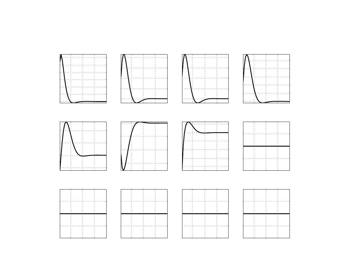
33
Figure 5. Shock to domestic demand (
ε
y
,ar
t
)
Output Gap (%)
10
20
30
40
0
0.2
0.4
0.6
0.8
1
1.2
Headline Inflation (QoQar %)
10
20
30
40
0
0.1
0.2
0.3
0.4
Core Inflation (QoQar %)
10
20
30
40
0
0.1
0.2
0.3
0.4
Policy Rate (%)
10
20
30
40
0
0.1
0.2
0.3
0.4
0.5
Real Interest Rate (%)
10
20
30
40
−0.1
0
0.1
0.2
Real Exchange Rate Gap (%)
10
20
30
40
−1.5
−1
−0.5
0
Nominal ER Depreciation (% ar)
10
20
30
40
−4
−3
−2
−1
0
1
Interbank Premium (%)
10
20
30
40
−1
−0.5
0
0.5
1
Output Gap EA (%)
10
20
30
40
−1
−0.5
0
0.5
1
Headline Inflation EA (QoQar %)
10
20
30
40
−1
−0.5
0
0.5
1
Policy Rate EA (%)
10
20
30
40
−1
−0.5
0
0.5
1
Interbank Premium EA (%)
10
20
30
40
−1
−0.5
0
0.5
1
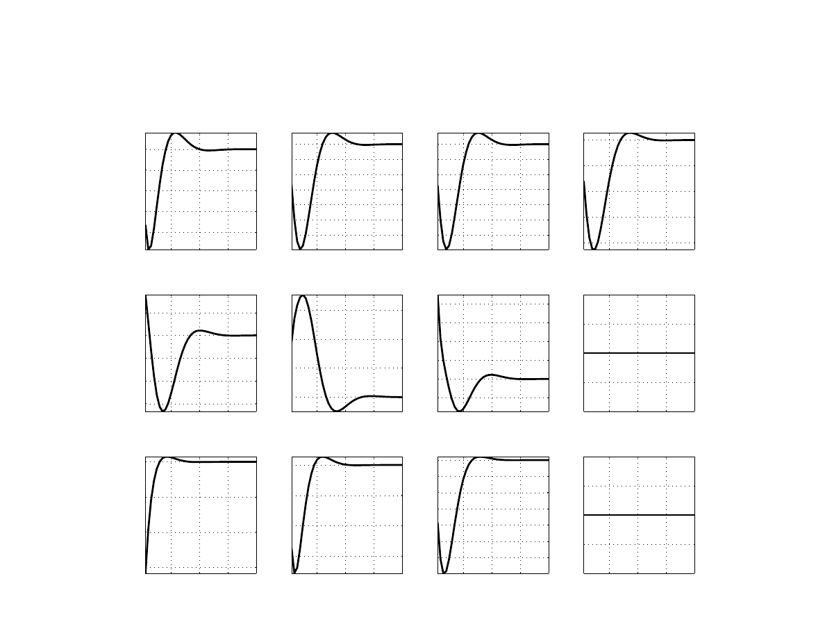
34
Figure 6. Negative shock to foreign demand (
ε
y
∗
,iid
t
)
Output Gap (%)
10
20
30
40
−0.4
−0.3
−0.2
−0.1
0
Headline Inflation (QoQar %)
10
20
30
40
−0.3
−0.25
−0.2
−0.15
−0.1
−0.05
0
Core Inflation (QoQar %)
10
20
30
40
−0.3
−0.25
−0.2
−0.15
−0.1
−0.05
0
Policy Rate (%)
10
20
30
40
−0.4
−0.3
−0.2
−0.1
0
Real Interest Rate (%)
10
20
30
40
−0.15
−0.1
−0.05
0
0.05
Real Exchange Rate Gap (%)
10
20
30
40
0
0.1
0.2
0.3
Nominal ER Depreciation (% ar)
10
20
30
40
−0.2
0
0.2
0.4
0.6
0.8
Interbank Premium (%)
10
20
30
40
−1
−0.5
0
0.5
1
Output Gap EA (%)
10
20
30
40
−1.5
−1
−0.5
0
Headline Inflation EA (QoQar %)
10
20
30
40
−0.3
−0.2
−0.1
0
Policy Rate EA (%)
10
20
30
40
−0.3
−0.25
−0.2
−0.15
−0.1
−0.05
0
Interbank Premium EA (%)
10
20
30
40
−1
−0.5
0
0.5
1
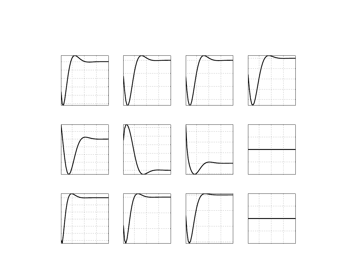
35
Figure 7. Negative global demand shock (
ε
com
t
)
Output Gap (%)
10
20
30
40
−2.5
−2
−1.5
−1
−0.5
0
Headline Inflation (QoQar %)
10
20
30
40
−1.5
−1
−0.5
0
Core Inflation (QoQar %)
10
20
30
40
−1.5
−1
−0.5
0
Policy Rate (%)
10
20
30
40
−2
−1.5
−1
−0.5
0
Real Interest Rate (%)
10
20
30
40
−0.8
−0.6
−0.4
−0.2
0
0.2
Real Exchange Rate Gap (%)
10
20
30
40
0
0.5
1
1.5
2
2.5
Nominal ER Depreciation (% ar)
10
20
30
40
−2
0
2
4
6
Interbank Premium (%)
10
20
30
40
−1
−0.5
0
0.5
1
Output Gap EA (%)
10
20
30
40
−3
−2.5
−2
−1.5
−1
−0.5
0
Headline Inflation EA (QoQar %)
10
20
30
40
−1
−0.5
0
Policy Rate EA (%)
10
20
30
40
−1.5
−1
−0.5
0
Interbank Premium EA (%)
10
20
30
40
−1
−0.5
0
0.5
1
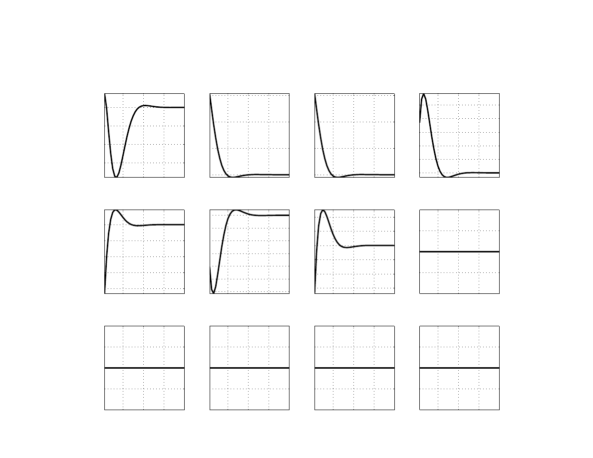
36
Figure 8. Shock to home core inflation (
ε
π
core
t
)
Output Gap (%)
10
20
30
40
−0.15
−0.1
−0.05
0
Headline Inflation (QoQar %)
10
20
30
40
0
0.5
1
1.5
Core Inflation (QoQar %)
10
20
30
40
0
0.5
1
1.5
Policy Rate (%)
10
20
30
40
0
0.1
0.2
0.3
0.4
0.5
Real Interest Rate (%)
10
20
30
40
−0.8
−0.6
−0.4
−0.2
0
Real Exchange Rate Gap (%)
10
20
30
40
−1.2
−1
−0.8
−0.6
−0.4
−0.2
0
Nominal ER Depreciation (% ar)
10
20
30
40
−1.5
−1
−0.5
0
0.5
1
Interbank Premium (%)
10
20
30
40
−1
−0.5
0
0.5
1
Output Gap EA (%)
10
20
30
40
−1
−0.5
0
0.5
1
Headline Inflation EA (QoQar %)
10
20
30
40
−1
−0.5
0
0.5
1
Policy Rate EA (%)
10
20
30
40
−1
−0.5
0
0.5
1
Interbank Premium EA (%)
10
20
30
40
−1
−0.5
0
0.5
1
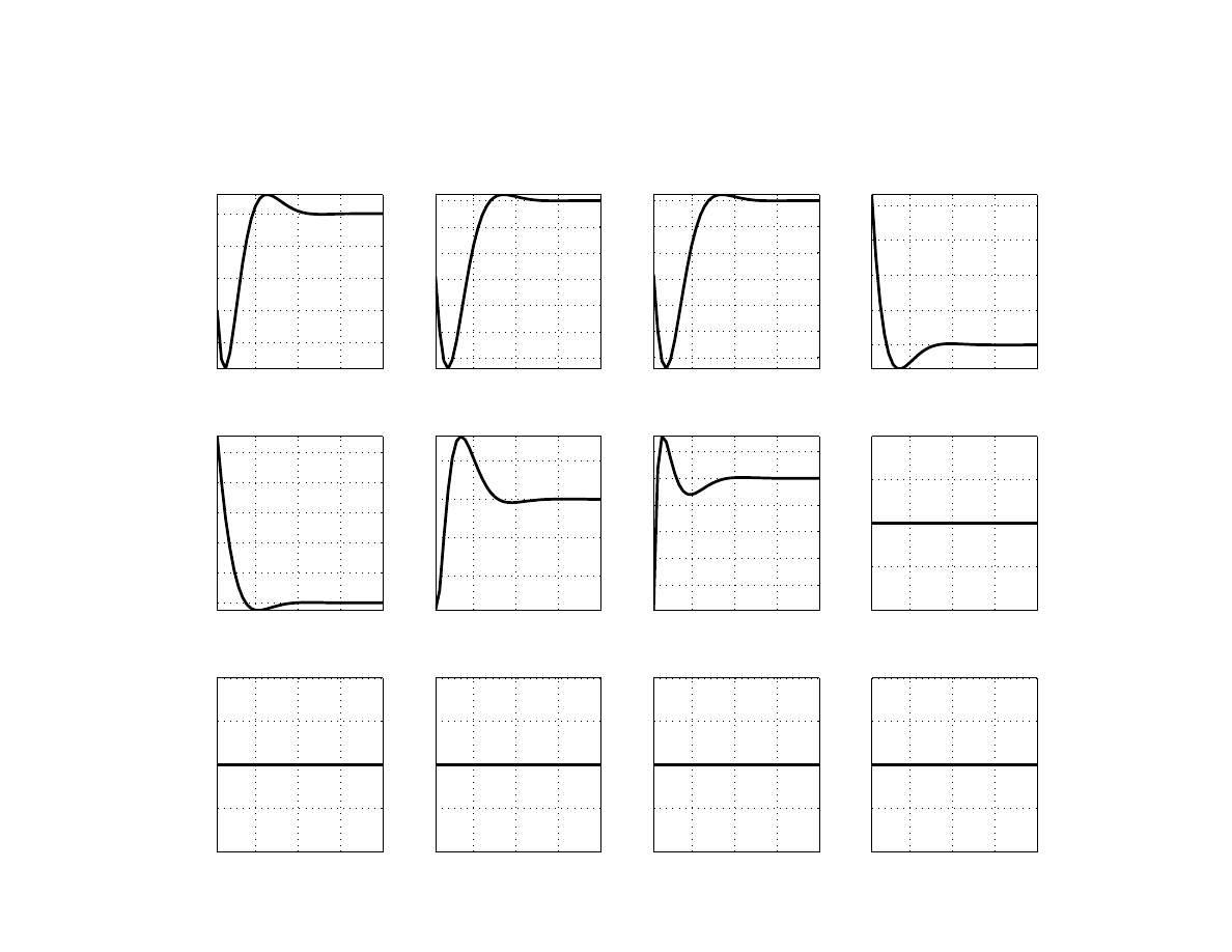
37
Figure 9. Shock to domestic monetary policy (
ε
I
t
)
Output Gap (%)
10
20
30
40
−0.2
−0.15
−0.1
−0.05
0
Headline Inflation (QoQar %)
10
20
30
40
−0.3
−0.25
−0.2
−0.15
−0.1
−0.05
0
Core Inflation (QoQar %)
10
20
30
40
−0.3
−0.25
−0.2
−0.15
−0.1
−0.05
0
Policy Rate (%)
10
20
30
40
0
0.2
0.4
0.6
0.8
Real Interest Rate (%)
10
20
30
40
0
0.2
0.4
0.6
0.8
1
Real Exchange Rate Gap (%)
10
20
30
40
−0.4
−0.2
0
0.2
Nominal ER Depreciation (% ar)
10
20
30
40
−2
−1.5
−1
−0.5
0
0.5
Interbank Premium (%)
10
20
30
40
−1
−0.5
0
0.5
1
Output Gap EA (%)
10
20
30
40
−1
−0.5
0
0.5
1
Headline Inflation EA (QoQar %)
10
20
30
40
−1
−0.5
0
0.5
1
Policy Rate EA (%)
10
20
30
40
−1
−0.5
0
0.5
1
Interbank Premium EA (%)
10
20
30
40
−1
−0.5
0
0.5
1
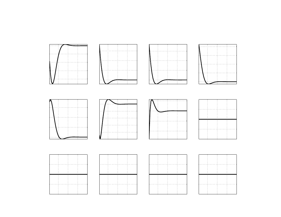
38
Figure 10. Permanent disinflation shock (
ε
π
tar
t
)
Output Gap (%)
10
20
30
40
−0.2
−0.15
−0.1
−0.05
0
Headline Inflation (QoQar %)
10
20
30
40
−1
−0.8
−0.6
−0.4
Core Inflation (QoQar %)
10
20
30
40
−1
−0.8
−0.6
−0.4
Policy Rate (%)
10
20
30
40
−1
−0.8
−0.6
−0.4
−0.2
Real Interest Rate (%)
10
20
30
40
0
0.1
0.2
0.3
Real Exchange Rate Gap (%)
10
20
30
40
−1
−0.8
−0.6
−0.4
−0.2
0
Nominal ER Depreciation (% ar)
10
20
30
40
−3
−2
−1
0
Interbank Premium (%)
10
20
30
40
−1
−0.5
0
0.5
1
Output Gap EA (%)
10
20
30
40
−1
−0.5
0
0.5
1
Headline Inflation EA (QoQar %)
10
20
30
40
−1
−0.5
0
0.5
1
Policy Rate EA (%)
10
20
30
40
−1
−0.5
0
0.5
1
Interbank Premium EA (%)
10
20
30
40
−1
−0.5
0
0.5
1
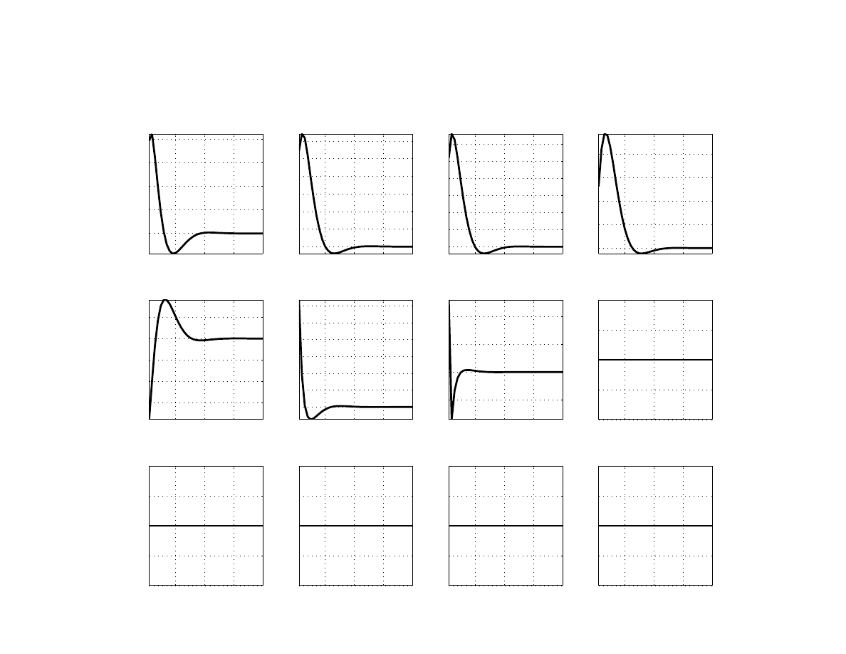
39
Figure 11. Shock to exchange rate (
ε
S
t
)
Output Gap (%)
10
20
30
40
0
0.05
0.1
0.15
0.2
Headline Inflation (QoQar %)
10
20
30
40
0
0.05
0.1
0.15
0.2
0.25
0.3
Core Inflation (QoQar %)
10
20
30
40
0
0.05
0.1
0.15
0.2
0.25
0.3
Policy Rate (%)
10
20
30
40
0
0.05
0.1
0.15
0.2
Real Interest Rate (%)
10
20
30
40
−0.15
−0.1
−0.05
0
0.05
Real Exchange Rate Gap (%)
10
20
30
40
0
0.5
1
1.5
2
2.5
3
Nominal ER Depreciation (% ar)
10
20
30
40
−5
0
5
10
Interbank Premium (%)
10
20
30
40
−1
−0.5
0
0.5
1
Output Gap EA (%)
10
20
30
40
−1
−0.5
0
0.5
1
Headline Inflation EA (QoQar %)
10
20
30
40
−1
−0.5
0
0.5
1
Policy Rate EA (%)
10
20
30
40
−1
−0.5
0
0.5
1
Interbank Premium EA (%)
10
20
30
40
−1
−0.5
0
0.5
1
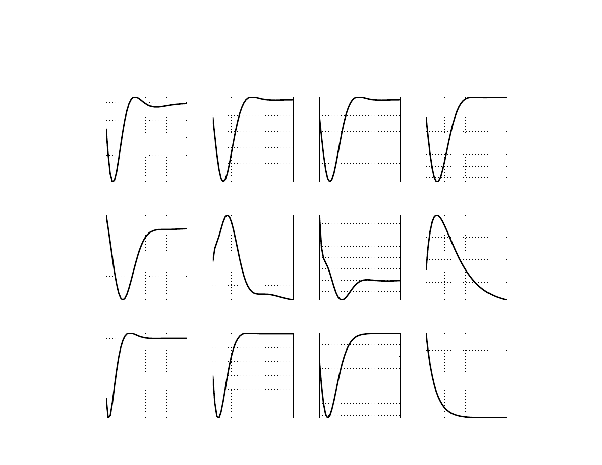
40
Figure 12. Shock to foreign interbank market premium (
ε
χ
∗
t
)
Output Gap (%)
10
20
30
40
−0.2
−0.15
−0.1
−0.05
0
Headline Inflation (QoQar %)
10
20
30
40
−0.25
−0.2
−0.15
−0.1
−0.05
0
Core Inflation (QoQar %)
10
20
30
40
−0.25
−0.2
−0.15
−0.1
−0.05
0
Policy Rate (%)
10
20
30
40
−0.35
−0.3
−0.25
−0.2
−0.15
−0.1
−0.05
Real Interest Rate (%)
10
20
30
40
−0.1
−0.05
0
Real Exchange Rate Gap (%)
10
20
30
40
0.05
0.1
0.15
0.2
0.25
Nominal ER Depreciation (% ar)
10
20
30
40
−0.1
0
0.1
0.2
0.3
0.4
0.5
Interbank Premium (%)
10
20
30
40
0.05
0.1
0.15
Output Gap EA (%)
10
20
30
40
−0.3
−0.2
−0.1
0
Headline Inflation EA (QoQar %)
10
20
30
40
−0.3
−0.25
−0.2
−0.15
−0.1
−0.05
0
Policy Rate EA (%)
10
20
30
40
−0.35
−0.3
−0.25
−0.2
−0.15
−0.1
−0.05
Interbank Premium EA (%)
10
20
30
40
0.2
0.4
0.6
0.8
1
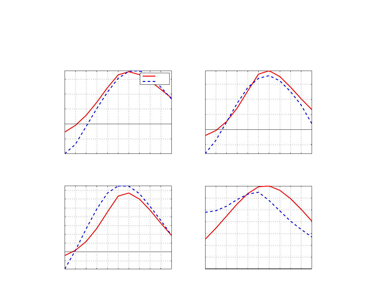
41
Figure 13. Output gap, core inflation and interest rates – Correlations (2000Q1 - 2012Q4)
−5
−4
−3
−2
−1
0
1
2
3
4
5
−0.2
0
0.2
0.4
0.6
PIE_CORE −−> Y(t−k)
model
data
−5
−4
−3
−2
−1
0
1
2
3
4
5
−0.2
0
0.2
0.4
0.6
PIE_CORE_EU −−> Y_EU(t−k)
−5
−4
−3
−2
−1
0
1
2
3
4
5
−0.1
0
0.1
0.2
0.3
0.4
0.5
0.6
0.7
Y −−> Y_EU(t−k)
−5
−4
−3
−2
−1
0
1
2
3
4
5
0
0.1
0.2
0.3
0.4
0.5
0.6
0.7
RS −−> RS_EU(t−k)
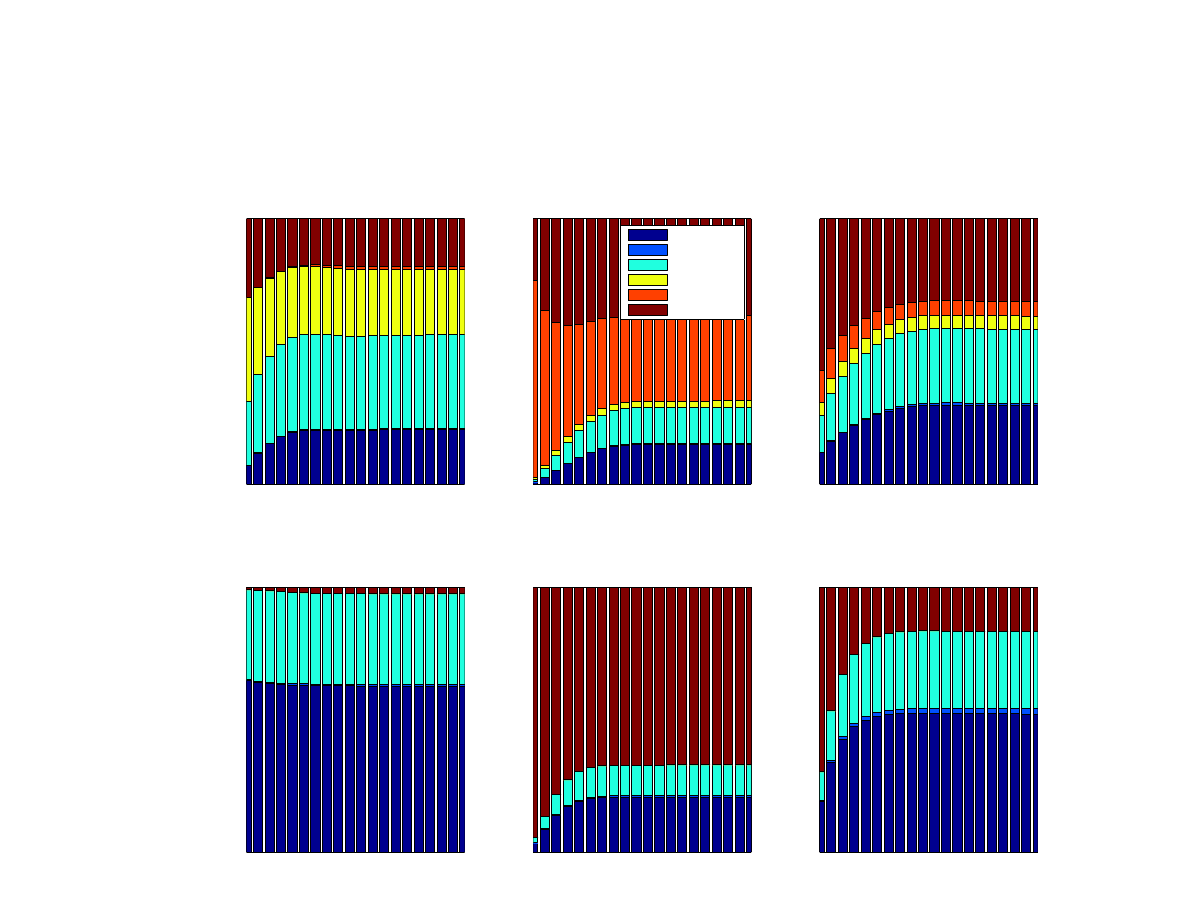
42
Figure 14. Forecast error variance decomposition for Poland and Euro area
5
10
15
20
0
0.1
0.2
0.3
0.4
0.5
0.6
0.7
0.8
0.9
1
Forecast horizon (quarters)
Output
5
10
15
20
0
0.1
0.2
0.3
0.4
0.5
0.6
0.7
0.8
0.9
1
Forecast horizon (quarters)
Inflation
EA demand
EA premium
Common
PL demand
PL costpush
rest
5
10
15
20
0
0.1
0.2
0.3
0.4
0.5
0.6
0.7
0.8
0.9
1
Forecast horizon (quarters)
Interest Rate
5
10
15
20
0
0.1
0.2
0.3
0.4
0.5
0.6
0.7
0.8
0.9
1
Forecast horizon (quarters)
EA Output
5
10
15
20
0
0.1
0.2
0.3
0.4
0.5
0.6
0.7
0.8
0.9
1
Forecast horizon (quarters)
EA Inflation
5
10
15
20
0
0.1
0.2
0.3
0.4
0.5
0.6
0.7
0.8
0.9
1
Forecast horizon (quarters)
EA Interest Rate
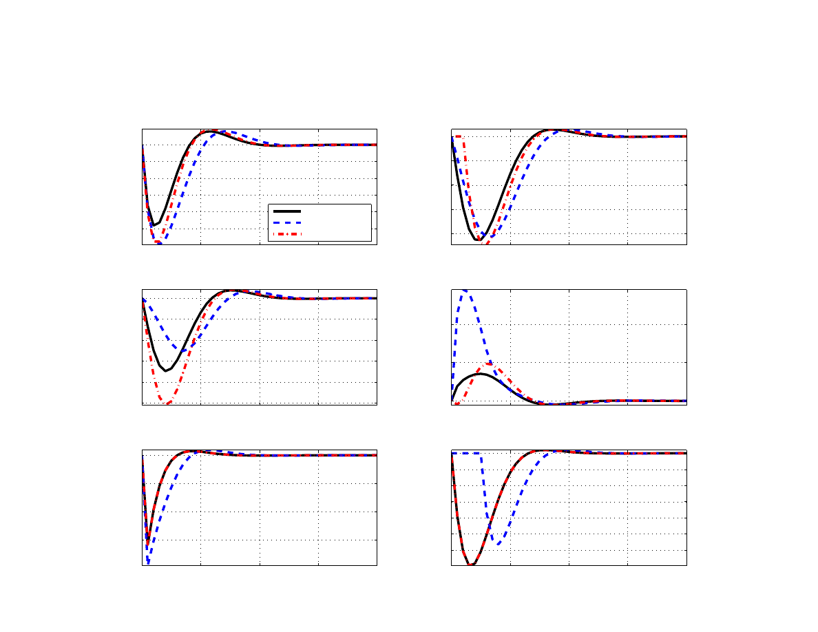
43
Figure 15. Counterfactual 1: Responses to euro area demand shock with monetary policy delay
Output Gap (%)
0
10
20
30
40
−0.5
−0.4
−0.3
−0.2
−0.1
0
Baseline
Policy delay EA
Policy delay PL
Policy Interest Rate (%)
0
10
20
30
40
−0.4
−0.3
−0.2
−0.1
0
CPI Inflation (QoQar %)
0
10
20
30
40
−0.5
−0.4
−0.3
−0.2
−0.1
0
Real Exchange Rate Gap (%)
0
10
20
30
40
0
0.5
1
Output Gap EA (%)
0
10
20
30
40
−1.5
−1
−0.5
0
Policy Interest Rate EA (%)
0
10
20
30
40
−0.3
−0.25
−0.2
−0.15
−0.1
−0.05
0
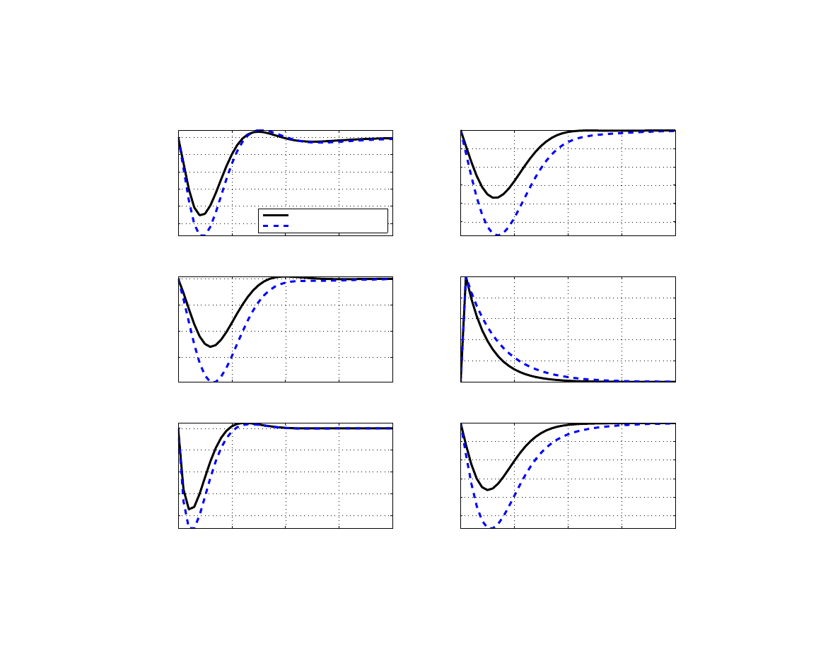
44
Figure 16. Counterfactual 2: Responses to euro area financial shock with higher shock persistence
Output Gap (%)
0
10
20
30
40
−0.25
−0.2
−0.15
−0.1
−0.05
0
Baseline
More persistent premium
Policy Interest Rate (%)
0
10
20
30
40
−0.5
−0.4
−0.3
−0.2
−0.1
0
CPI Inflation (QoQar %)
0
10
20
30
40
−0.3
−0.2
−0.1
0
Interbank Premium EA (%)
0
10
20
30
40
0
0.2
0.4
0.6
0.8
1
Output Gap EA (%)
0
10
20
30
40
−0.4
−0.3
−0.2
−0.1
0
Policy Interest Rate EA (%)
0
10
20
30
40
−0.5
−0.4
−0.3
−0.2
−0.1
0
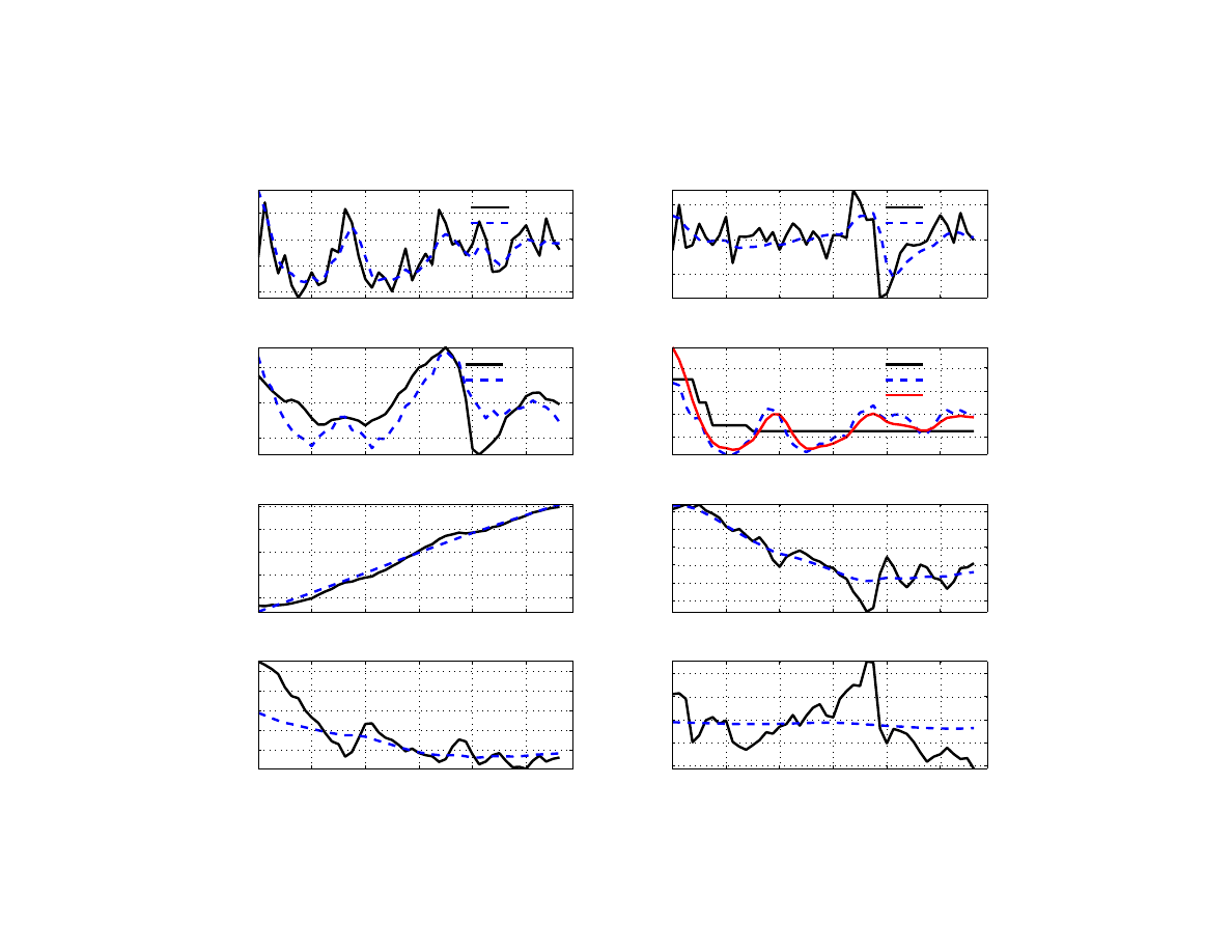
45
Figure 17. Estimated output gap, core inflation, and equilibrium variables
Poland: Inflation (QoQar %),
2001:1
2003:1
2005:1
2007:1
2009:1
2011:1
0
2
4
6
Headline
"Core"
Euro area: Inflation (QoQar %)
2001:1
2003:1
2005:1
2007:1
2009:1
2011:1
0
2
4
Headline
"Core"
Home and Foreign Output Gap (%)
2001:1
2003:1
2005:1
2007:1
2009:1
2011:1
−2
0
2
Euro area
Poland
Poland: Inflation and Target (YoY %)
2001:1
2003:1
2005:1
2007:1
2009:1
2011:1
2
4
6
8
Target
Headline
"Core"
Poland: (Log) GDP and Trend GDP
2001:1
2003:1
2005:1
2007:1
2009:1
2011:1
540
550
560
570
580
Poland: (Log) Actual and Trend Real Exchange Rate
2001:1
2003:1
2005:1
2007:1
2009:1
2011:1
−20
0
20
40
60
80
Poland: Actual and Trend Real Interest Rate (%)
2001:1
2003:1
2005:1
2007:1
2009:1
2011:1
2
4
6
8
10
Euro area: Actual and Trend Real Interest Rate (%)
2001:1
2003:1
2005:1
2007:1
2009:1
2011:1
−1
0
1
2
3
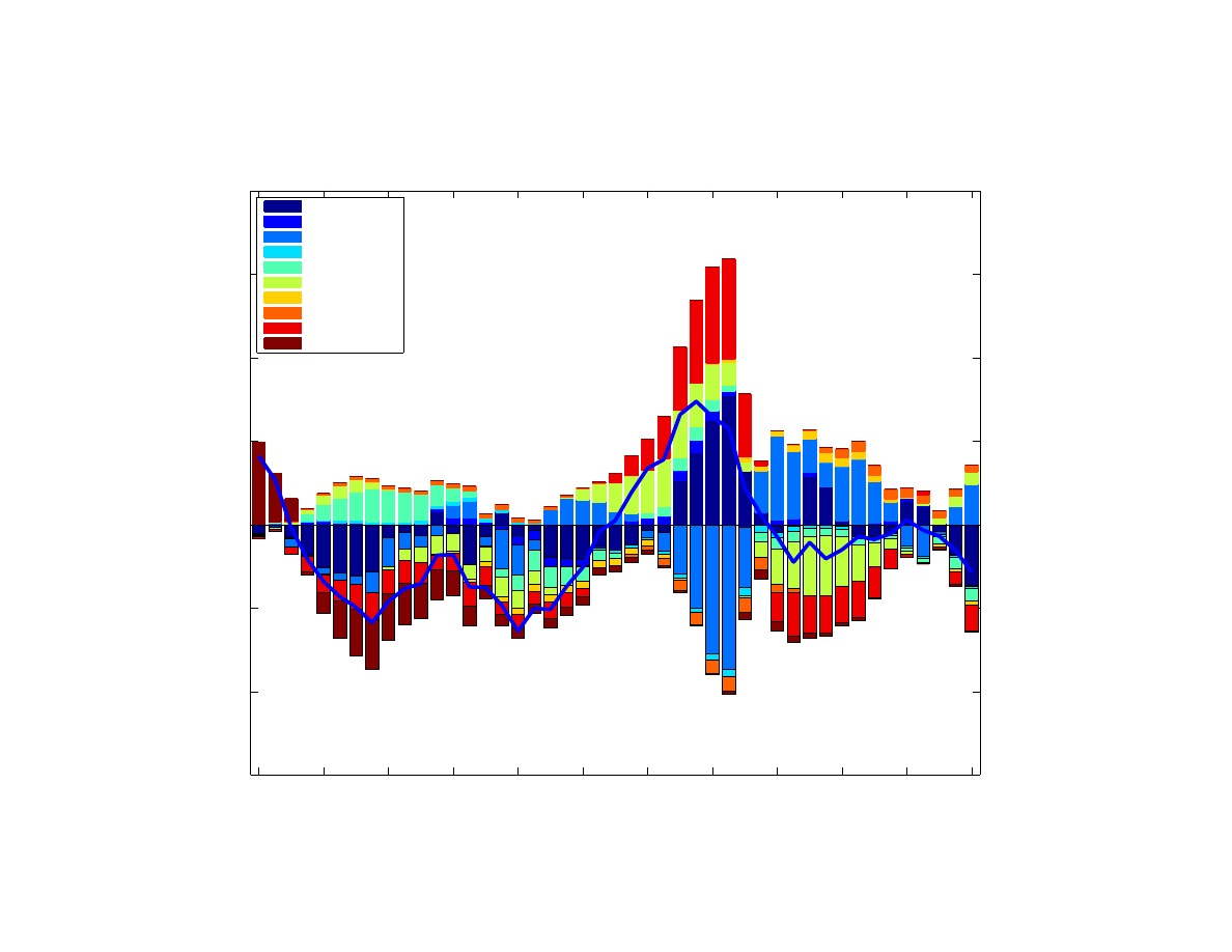
46
Figure 18. Historical shock decomposition - Output
2001:2
2002:2
2003:2
2004:2
2005:2
2006:2
2007:2
2008:2
2009:2
2010:2
2011:2
2012:2
−6
−4
−2
0
2
4
6
8
Output Gap (percent)
demand
MP+premium
exchange rate
oil
costpush
EA demand
EA costpush
EA MP+premium
common
−rest−
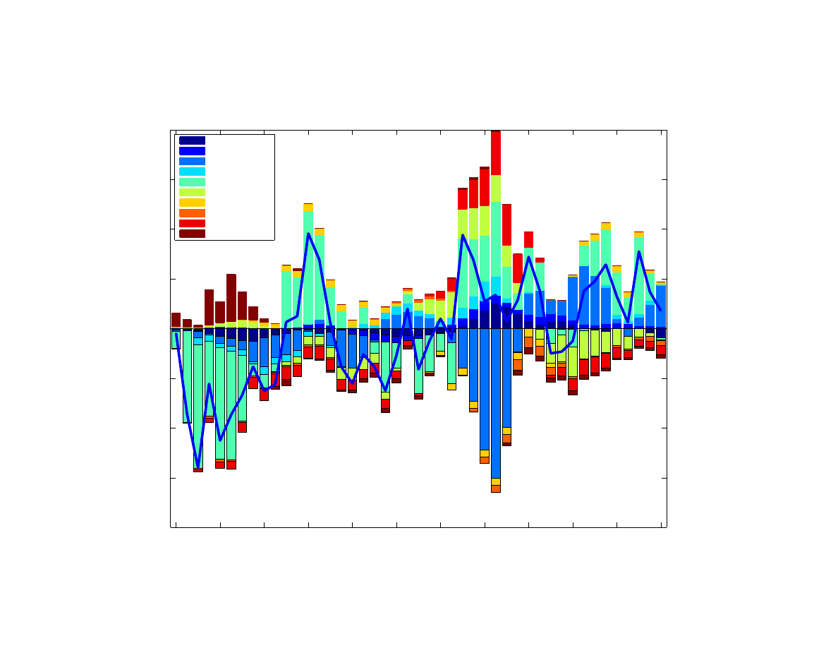
47
Figure 19. Historical shock decomposition - Inflation
2001:2
2002:2
2003:2
2004:2
2005:2
2006:2
2007:2
2008:2
2009:2
2010:2
2011:2
2012:2
−8
−6
−4
−2
0
2
4
6
8
Inflation (deviation from target, percent)
demand
MP+premium
exchange rate
oil
costpush
EA demand
EA costpush
EA MP+premium
common
−rest−
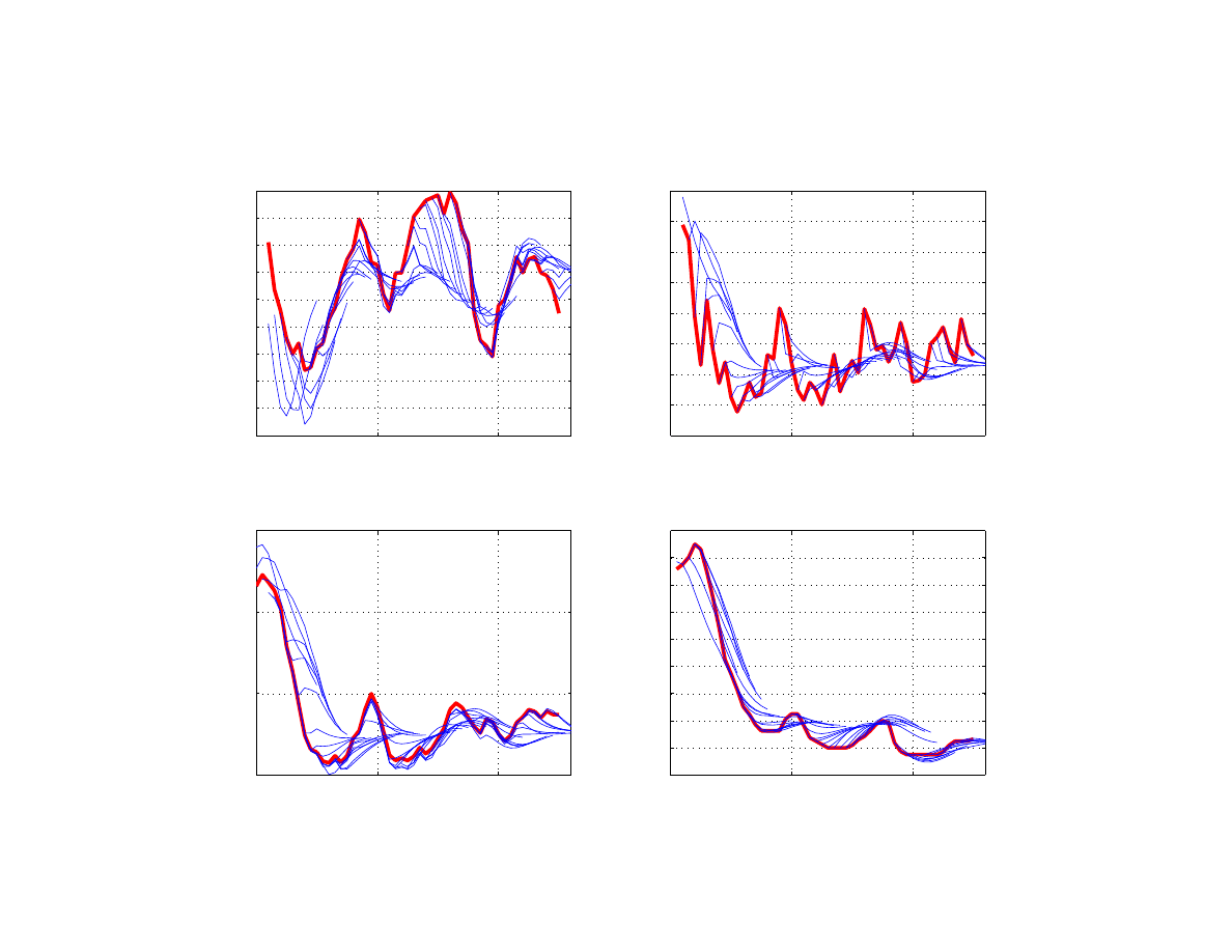
48
Figure 20. Conditional in-sample forecast (8 quarters ahead)
1999:4
2004:4
2009:4
−2
−1
0
1
2
3
4
5
6
7
Output Growth
1999:4
2004:4
2009:4
−2
0
2
4
6
8
10
12
14
Inflation
1999:4
2004:4
2009:4
0
5
10
15
Core Inflation
1999:4
2004:4
2009:4
2
4
6
8
10
12
14
16
18
20
Interest Rate
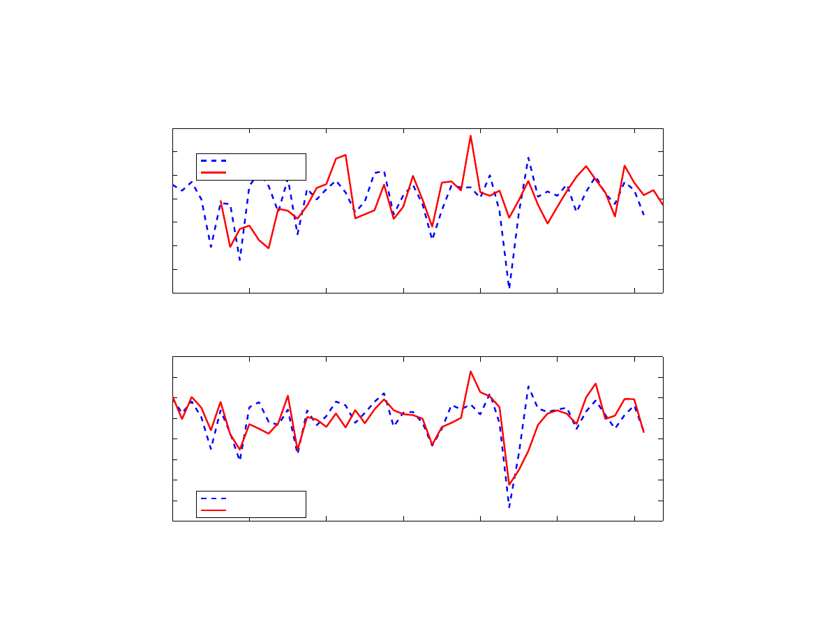
49
Figure 21. Non-core “wedge” and oil prices
2000:1
2002:1
2004:1
2006:1
2008:1
2010:1
2012:1
−4
−3
−2
−1
0
1
2
3
Poland
Oil inflation (YoY %)
Oil "wedge" (%)
2000:1
2002:1
2004:1
2006:1
2008:1
2010:1
2012:1
−5
−4
−3
−2
−1
0
1
2
3
Euro Area
Oil inflation (YoY %)
Oil "wedge" (%)
Document Outline
Wyszukiwarka
Podobne podstrony:
[Karl Cordell] Germany, Poland and the Czech Repub(BookZZ org)
Mark Paul A Tangled Web Polish Jewish Relations in Wartime Northeastern Poland and the Aftermath Pa
Independence Day, Myth, Symbol, and the Creation of Modern Poland
The?termath of Euro 2012 Spain, Poland and Ukraine
An Analysis of Euro Area Sovereign CDS and their Relation with Government Bonds
Independence Day, Myth, Symbol, and the Creation of Modern Poland
Wójcik, Marcin Rural space and the concept of modernisation Case of Poland (2014)
Kulesza, Mariusz; Kaczyńska, Dorota Multinational cultural heritage of the Eastern part of the Comm
Wójcik, Marcin Peripheral areas in geographical concepts and the context of Poland s regional diver
Hiding data inside the padding area in files and packets
Edward Elgar Publishing The Euro Its Origins, Development and Prospects
Mettern S P Rome and the Enemy Imperial Strategy in the Principate
Diet, Weight Loss and the Glycemic Index
Ziba Mir Hosseini Towards Gender Equality, Muslim Family Laws and the Sharia
pacyfic century and the rise of China
Danielsson, Olson Brentano and the Buck Passers
Japan and the Arctic not so Poles apart Sinclair
Pappas; Routledge Philosophy Guidebook to Plato and the Republic
więcej podobnych podstron