ENVI Tutorial:
Atmospherically Correcting
Multispectral Data Using
FLAASH

Atmospherically Correcting Multispectral Data Using FLAASH

2

Files Used in this Tutorial

2

Opening the Raw Landsat Image in ENVI

3

Preparing the Image for Use in FLAASH

4

Calibrating the TM Image into Radiance

4

Adjusting the Radiance Units

4

Converting the Interleave

5

Atmospherically Correcting the TM Image Using FLAASH

6

Viewing the Corrected Image

9

Verify the Model Results

10

Comparing Images

10

Computing a Difference Image Using Band Math

10

1

Atmospherically Correcting Multispectral Data
Using FLAASH

This tutorial provides an introduction to using FLAASH (included in the Atmospheric Correction
Module: QUAC and FLAASH) to atmospherically correct a multispectral image. You will display the
radiance image, prepare the data for use in FLAASH, apply an atmospheric correction, and examine the
results.

In order to run this tutorial, you must have ENVI and the Atmospheric Correction Module: QUAC and
FLAASH installed on your computer.

Files Used in this Tutorial

ENVI Resource DVD:

Data\flaash\multispectral\input_files (radiance image, scale factors file, and
template file)

Data\flaash\multispectral\flaash_results (sample reflectance image)
The image used in this exercise was collected by the Landsat 7 ETM+ sensor on April 3, 1997. It is a
standard L1G product. It is a spatial subset of a full Landsat TM scene for path 44 row 34. The image
covers a portion of the Jasper Ridge Biological Preserve, located in the eastern foothills of the Santa
Cruz Mountains at the base of the San Francisco Peninsula, nine kilometers west of the main Stanford
University campus in San Mateo County, CA. The Landsat image was provided courtesy of the USGS
EROS Data Center. The full scene is available at

http://glovis.usgs.gov

. This image contains

approximately the same area as the AVIRIS image used for the FLAASH hyperspectral tutorial,
however the pixel size, image orientation, and collection dates are different.

File

Description

LandsatTM_JasperRidge_B10.FST

FLAASH input images: Landsat 7 ETM+
fast format Level 1G data product

LandsatTM_JasperRidge_B20.FST

LandsatTM_JasperRidge_B30.FST

LandsatTM_JasperRidge_B40.FST

LandsatTM_JasperRidge_B50.FST

LandsatTM_JasperRidge_B70.FST

LandsatTM_JasperRidge_HRF.FST

JasperRidgeTM_template.txt

FLAASH template file

JasperRidgeTM_flaash_refl.img

FLAASH reflectance result

2

ENVI Tutorial: Atmospherically Correcting Multispectral Data
Using FLAASH

ENVI Tutorial: Atmospherically Correcting Multispectral Data

Using FLAASH

Opening the Raw Landsat Image in ENVI

This exercise will demonstrate how to use FLAASH to produce an apparent surface reflectance image.

1. From the ENVI main menu bar, select File > Open External File > Landsat > Fast.

2. Navigate to the Data\flaash\multispectral\input_files directory, select the

LandsatTM_JasperRidge_HRF.FST header file from the list, and click Open. The
Available Bands List is displayed.

3. From the Available Bands List, right-click on the LandsatTM_JasperRidge_HRF.FST file

and select Load True Color. The image is loaded into the display.

You may recognize several features in the scene, including a long lake oriented NW-SE in the
middle of the image, various types of vegetation on the left hand side of the image, and urban
areas on the right-hand side.

This image is a standard Landsat-7 L1G data product, except that it has been spatially subsetted
to a small area around Jasper Ridge. The data type is byte (8 bits per pixel), and the image
contains uncalibrated digital numbers (or DN).

4. From the Display group menu bar, select Enhance > [Image] Gaussian to enhance the display.

3

Preparing the Image for Use in FLAASH

Before the TM image can be corrected using FLAASH, it must be calibrated into the proper radiance
units and converted into a BIP or BIL interleave.

Calibrating the TM Image into Radiance

FLAASH requires that the input image be calibrated into radiance in units of [μW/(cm

2

*sr*nm)]. This

can be accomplished in two simple steps using standard ENVI utilities.

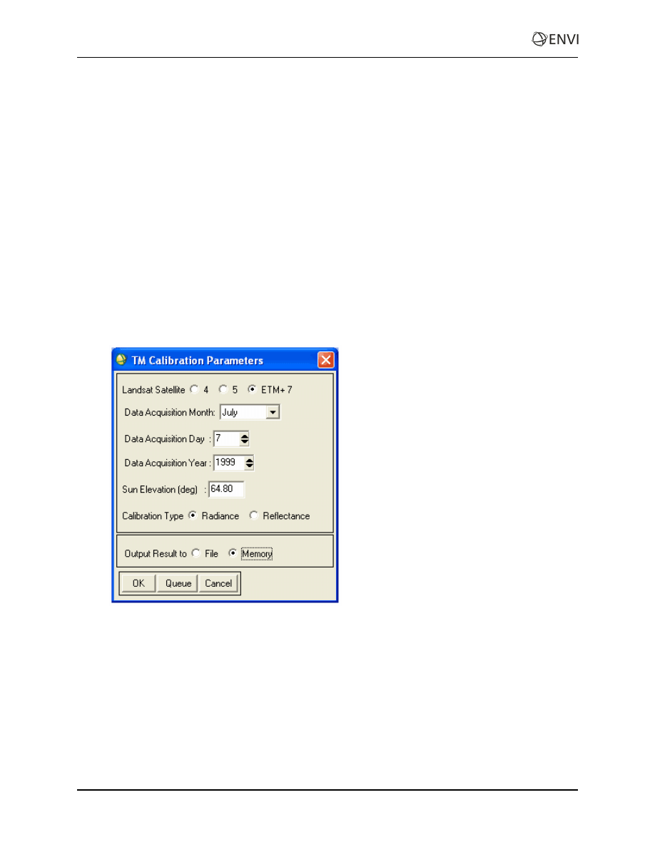
1. From the ENVI main menu bar, select Basic Tools > Preprocessing > Calibration Utilities >

Landsat TM. The TM Calibration Input File dialog appears.

2. Select the LandsatTM_JasperRidge_hrf.fst file and click OK. The TM Calibration

Parameters dialog appears.

3. Click the Radiance Calibration Type radio button.

4. Click the Memory radio button, and click OK. The new bands are loaded into the Available

Bands List.

Adjusting the Radiance Units

ENVI’s TM/ETM+ calibration utility outputs data with radiance units of [W/(m

2

*sr*μm)]. However,

FLAASH requires radiance in units of [μW/(cm

2

*sr*nm)]. These two units differ by a factor of 10, so

an additional step is required to convert the units. This exercise uses Band Math to divide the radiance
units by 10.

1. From the ENVI main menu bar, select Basic Tools > Band Math.

2. In the Enter an expression field, type the expression:

b1 / 10.0

4

ENVI Tutorial: Atmospherically Correcting Multispectral Data
Using FLAASH

ENVI Tutorial: Atmospherically Correcting Multispectral Data

Using FLAASH

3. Click OK. The Variables to Bands Pairings dialog appears.

4. Click Map Variable to Input File. The Band Math Input File dialog appears.

5. Select the [Memory1] input file, and click OK.

6. In the Enter Output Filename field, type JasperRidgeTM_radiance.img and click Open.

7. Click OK in the Variables to Bands Pairings dialog. The new bands are loaded into the Available

Bands List.

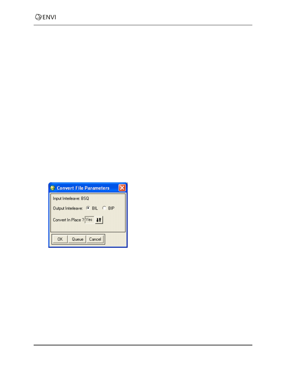
Converting the Interleave

The Band Math result from the previous step has a BSQ interleave, but FLAASH requires the input
radiance image to be in either BIL or BIP interleave.

1. From the ENVI main menu bar, select Basic Tools > Convert Data (BSQ, BIL, BIP). The

Convert File Input File dialog appears.

2. Select the JasperRidgeTM_radiance.img file and click OK. The Convert File Parameters dialog

appears.

3. Click the BIL Output Interleave radio button.

4. Click the Convert in Place toggle button to select Yes, click OK to start processing, and answer

Yes to the warning message. For relatively small files such as this, it is faster to perform the
interleave conversion in place. For larger images, such as a full Landsat TM scene, it will be
considerably faster to write the new interleave file to disk.

5

Atmospherically Correcting the TM Image Using
FLAASH

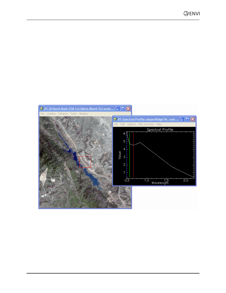
1. From the Available Bands List, right-click on the JasperRidgeTM_radiance.img file and

select Load True Color to <current>.

2. From the Display group menu bar, select Enhance > [Image] Gaussian to enhance the display.

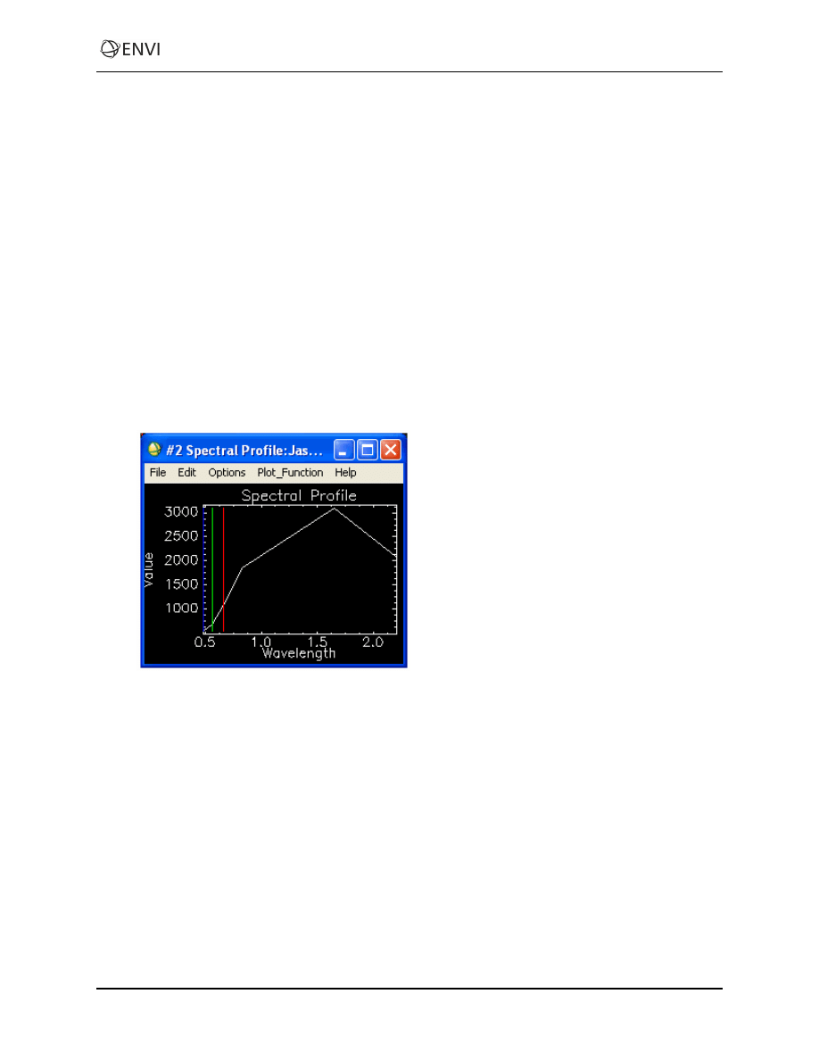
3. Right-click in the Image window and select Z Profile (Spectrum) to display the Spectral Profile.

4. Click and drag in the bottom middle part of the image over the vegetated areas, and note the shape

of the radiance curves. The most prominent atmospheric feature in these spectra is the consistent
upward trend in the blue and green bands. This is likely caused by atmospheric aerosol scattering,
or what is often referred to as ‘skylight’. An accurate atmospheric correction should compensate
for the skylight to produce spectra that more truly depict surface reflectance.

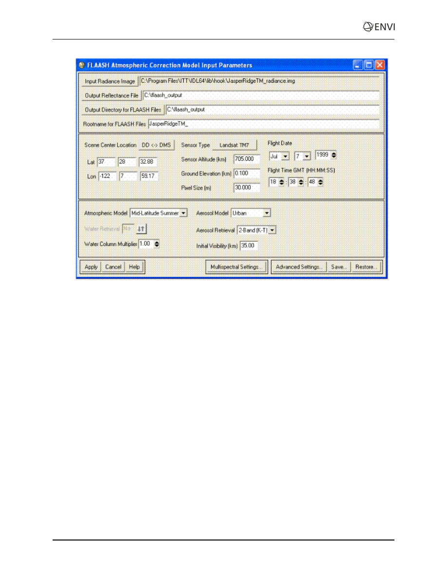
5. From the ENVI main menu bar, select Spectral > FLAASH. The FLAASH Atmospheric

Correction Model Input Parameters dialog appears.

6. Click the Input Radiance Image button, select the JasperRidgeTM_radiance.img file,

and click OK. The Radiance Scale Factors dialog appears.

7. Select the Use single scale factor for all bands radio button. Since the input image units have

already been correctly scaled (see "Preparing the Image for Use in FLAASH" on page 4), the
Single Scale Factor default value of 1 is acceptable. If the units had not already been scaled, you
would enter a single scale factor of 10. Click OK.

6

ENVI Tutorial: Atmospherically Correcting Multispectral Data
Using FLAASH

ENVI Tutorial: Atmospherically Correcting Multispectral Data

Using FLAASH

8. In the Output Reflectance File field, type the full path of the directory where you want to write

the FLAASH-corrected output reflectance file. To navigate to the desired output directory before
defining the output file name, click the Output Reflectance File button.

9. In the Output Directory for FLAASH Files field, type the full path of the directory where you

want to have all other FLAASH output files written, along with a file name of your choice. You
may also click the Output Directory for FLAASH Files button to navigate to the desired
directory.

10. In the Rootname for FLAASH Files field, type the name you want to use as a prefix for the

FLAASH Output Files. In the next step, ENVI will automatically add an underscore character to
the rootname that you enter.

11. If Water Retrieval is selected, the FLAASH output files will consist of the column water vapor

image, the cloud classification map, the journal file, and (optionally) the template file. All of
these files are written into the FLAASH output directory and use the rootname as a prefix to their
individual standard filenames.

12. Click the Restore button.

13. Navigate to the Data\flaash\multispectral\input_files directory, select the

JasperRidgeTM_template.txt file, and click Open. This file provides the FLAASH
model parameters for the Jasper Ridge image. Review the scene collection details and model
parameters for the Jasper Ridge TM image.

In this example, the Water Retrieval toggle is set to No because the Landsat TM sensor does not
have bands in the water absorption regions that can be used to compute the atmospheric water
vapor. As is common for multispectral sensors, a fixed water amount based on a typical
atmosphere must be used instead.

7

14. Click the Multispectral Settings button to explore the multispectral settings variable. The

Multispectral Settings dialog is used to select a filter function file and define the bands that are
used for various FLAASH processing steps. The water retrieval bands are left undefined because
water retrieval is not possible with Landsat TM data. However, the Landsat TM sensor does
contain bands that can be used to estimate the aerosol concentration.

15. Click the Kaufman-Tanre Aerosol Retrieval tab in the Multispectral Settings dialog to see

which bands were selected.

16. Click Cancel to dismiss this dialog and return to the previous dialog.

17. Click the Advanced Settings button to explore the available advanced settings options. The

parameters in the Advanced Settings dialog allow you to adjust additional controls for the
FLAASH model. The default setting for Automatically Save Template File is Yes, and the
default for Output Diagnostic Files is No. While you may find it excessive to save a template
file for each FLAASH run, this file is often the only way to determine the model parameters that
were used to atmospherically correct an image after the run is complete, and access to it can be
quite important. The ability to output diagnostic files is offered solely as an aid for ENVI
Technical Support engineers to help diagnose problems.

18. Click Cancel to dismiss this dialog and return to the previous dialog.

19. In the FLAASH Atmospheric Model Input Parameters dialog, click Apply to begin the FLAASH

processing. You may cancel the processing at any point, but be aware that there are some
FLAASH processing steps that can’t be interrupted, so the response to the Cancel button may not
be immediate.

8

ENVI Tutorial: Atmospherically Correcting Multispectral Data
Using FLAASH

ENVI Tutorial: Atmospherically Correcting Multispectral Data

Using FLAASH

Viewing the Corrected Image

When FLAASH processing completes, the output reflectance image will be entered into the Available
Bands List. You should also find the journal file and the template file in the FLAASH output directory.

1. Click Cancel on the FLAASH Atmospheric Correction Model Input Parameters dialog to dismiss

the dialog.

2. Examine, then close, the FLAASH Atmospheric Correction Results dialog.

3. From the Available Bands List right-click on the JasperRidgeTM_radiance_

flaash.img file and select Load True Color to <new>. The image is loaded into a new
display group.

4. Right-click in the new Image window and select Z Profile (Spectrum) to display the Spectral

Profile.

5. Click and drag around the image and note the shape of the radiance curves. The vegetation

reflectance curves now display a more characteristic shape, with a peak in the green, a
chlorophyll absorption in the red, and a sharp red edge leading to higher near infrared reflectance.

9

Verify the Model Results

The results you produce with the sample Jasper Ridge files should be identical to the data found in the
Data\flaash\multispectral\flaash_results directory.

Comparing Images

1. From the ENVI main menu bar, select File > Open Image File.

2. Navigate to the Data\flaash\multispectral\flaash_results directory, select the

JasperRidgeTM_flaash_refl.img file and click Open. The Available Bands List is
displayed.

3. From the Available Bands List, right-click on the JasperRidgeTM_flaash_refl.img file

and select Load True Color to <new>. The image is loaded into a new display group.

4. From the Display group menu bar, select Tools > Link > Link Displays. You can also right-click

in the image and select Link Displays.

5. Toggle the Dynamic Overlay option Off, and click OK in the Link Displays dialog to establish

the link.

6. Double-click in one of the Image windows to display the Cursor Location/Value window.

7. Move your mouse cursor around in one of the images, and note the data values in the Cursor

Location/Value window. You should see that the data values are identical for corresponding
bands in both images.

Computing a Difference Image Using Band Math

For a more quantitative verification of the reflectance results, you will compute a difference image using
Band Math.

1. From the ENVI main menu bar, select Basic Tools > Band Math. The Band Math dialog

appears.

2. In the Enter an expression field, type the following expression:

float(b1) – b2

3. Click on B1 to select it, then click Map Variable to Input File. The Band Math Input File dialog

appears.

4. Select the JasperRidgeTM_flaash_refl.img file and click OK.
5. Click on B2 to select it, then click Map Variable to Input File. The Band Math Input File dialog

appears.

6. Select the JasperRidgeTM_radiance_flaash.img file and click OK.
7. In the Enter Output Filename field, type or choose a file name for the output result and click

OK. Note that the file size for this difference image will be twice as large as the FLAASH
reflectance image file, so be sure you have sufficient disk space for this Band Math result.

10

ENVI Tutorial: Atmospherically Correcting Multispectral Data
Using FLAASH

ENVI Tutorial: Atmospherically Correcting Multispectral Data

Using FLAASH

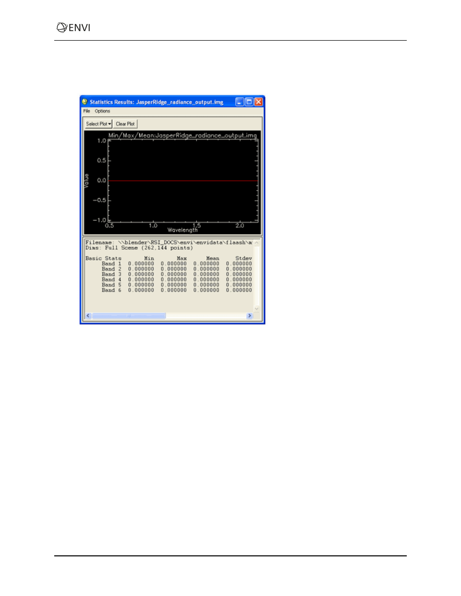
8. Every value in the difference image should be 0. To ensure that the results are identical, select

Basic Tools > Statistics > Compute Statistics from the ENVI main menu bar to calculate the
basic statistics for the difference image.

9. Note the Max and Min columns in the statistics report window.

10. Due to differences in computer machine precision, your FLAASH reflectance image result may

differ from those in the verification directory by approximately 1 to 5 DNs, or 0.0001 to 0.0005
reflectance units.

11. When you are finished comparing the results, exit ENVI by selecting File > Exit from the ENVI

main menu bar.

11