I. INTRODUCTION

In order to linearize general nonlinear systems, we will

use the Taylor Series expansion of functions. Consider a
function f(x) of a single variable x, and suppose that

x

is a

point such that f(

x

) = 0. In this case, the point

x

is called

an equilibrium point of the system

( ),

x

f x

=



since we have

0

x

=



when

x

x

=

(i.e., the system reaches an equilibrium

at

x

). Recall that the Taylor Series expansion of f(x) around

the point

x

is given by,,

2

2

2

1

( )

( )

(

)

2

(

)

... .

x x

x x

f

f

f x

f x

x

x

x

x

x

x

=

=





∂

∂





=

−

− − 











∂

∂









−

−

This can be written as

( )

( )

(

)

x x

f

f x

f x

x

x

x

=

∂





=

−

− −





∂





higher order terms.

For x sufficiently close to

,

x these higher order terms

will be very close to zero, and so we can drop them to
obtain the approximation

( )

( )

(

),

f x

f x

a x

x

≈

−

−

where

x x

f

a

x

=

∂





=  

∂





Since

( )

0,

f x

=

the nonlinear differential equation

( )

x

f x

=



can be approximated near the equilibrium point

by

(

)

x

a x

x

=

−



To complete the linearization, we define the perturbation

state (also known as delta state)

,

x

x

x

δ = −

and using the

fact that

,

x

x

δ =



 we obtain the linearized model

x

a x

δ = δ



This linear model is valid only near the equilibrium point.

II. EQUILIBRIUM POINTS

Consider a nonlinear differential equation

( )

[ ( ), ( )]

x t

f x t u t

=



... (1)

where

:

.

n

m

n

f R

R

R

×

→

A point

n

x

R

∈

is called an

equilibrium point if there is a specific

m

u

R

∈

(called the

equilibrium input) such that

( , )

0 .

n

f x u

=

Suppose

x

is an equilibrium point (with equilibrium

input

u

). Consider starting system (1) from initial condition

0

( )

,

x t

x

=

and applying the input

( )

u t

u

≡

for all

0

.

t

t

≥

The

resulting solution x(t) satisfies

( )

;

x t

x

−

for all

0

.

t

t

≥

That

is why it is called an equilibrium point.

III. DEVIATION VARIABLES

Suppose

( , )

x u

is an equilibrium point and input. Wee

know that if we start the system at

0

( )

,

x t

x

=

and apply the

constant input

( )

,

u t

u

≡

then the state of the system will

remain fixed at

( )

x t

x

=

for all t. Define deviation variables

to measure the difference.

( )

( )

and

( )

( )

x

x

t

x t

x

t

u t

u

δ

=

−

δ

=

−

In this way, we are simply relabling where we call 0.

Now, the variables x(t) and u(t) are related by the differential
equation

( )

[ ( ), ( )]

x t

f x t u t

=



Substituting in, using the constant and deviation

variables, we get

Linearization of Nonlinear Differential Equation by Taylor’s Series

Expansion and Use of Jacobian Linearization Process

M. Ravi Tailor* and P.H. Bhathawala**

*Department of Mathematics, Vidhyadeep Institute of Management and Technology, Anita, Kim, India

**S.S. Agrawal Institute of Management and Technology, Navsari, India

(Received 11 March, 2012, Accepted 12 May, 2012)

ABSTRACT : In this paper, we show how to perform linearization of systems described by nonlinear differential
equations. The procedure introduced is based on the Taylor's series expansion and on knowledge of Jacobian
linearization process. We develop linear differential equation by a specific point, called an equilibrium point.

Keywords : Nonlinear differential equation, Equilibrium Points, Jacobian Linearization, Taylor's Series Expansion.

International Journal of Theoretical and Applied Science 4(1): 36-38(2011)

International Journal of Theoretical & Applied Sciences, 1(1): 25-31(2009)

ISSN No. (Print) : 0975-1718

ISSN No. (Online) : 2249-3247

Tailor and Bhathawala

( )

[

( ),

( )]

x

x

x

t

f x

t u

t

δ

=

− δ

− δ



This is exact. Now however, let's do a Taylor expansion

of the right hand side, and neglect all higher (higher than
1st) order terms

( )

( , )

( )

( )

x

x x

x

x x

u

u u

u u

f

f

t

f x u

t

t

x

u

=

=

=

=

∂

∂

δ

≈

−

δ

−

δ

∂

∂



But

( , )

0,

f x u

=

( )

( )

( )

x

x x

x

x x

u

u u

u u

f

f

t

t

t

x

u

=

=

=

=

∂

∂

δ

≈

δ

−

δ

∂

∂



This differential equation approximately governs (we are

neglecting 2

nd

order and Higher order terms) the deviation

variables

( )

x

t

δ

and

( ),

u

t

δ

as long as they remain small. It

is a linear, time-invariant, differential equation, since the

derivatives of

x

δ

are linear combinations of the

x

δ

variables

and the deviation inputs,

.

u

δ

The matrices,

,

n

n

x x

u u

f

A

R

R

x

=

=

∂

=

∈

×

∂

n

m

x x

u u

f

B

R

R

u

=

=

∂

=

∈

×

∂

... (2)

are constant matrices. With the matrices A and B as

defined in (2), the linear system

( )

( )

( )

x

x

u

t

A

t

B

t

δ

≈ δ

− δ



is called the Jacobian Linearization of the original

nonlinear system (1), about the equilibrium point

( , ).

x u

For

“small” values of

x

δ

and

,

u

δ

the linear equation

approximately governs the exact relationship between the

deviation variables

x

δ

and

.

u

δ

For “small”

x

δ

[i.e., while u(t) remains close to

],

u

and while

x

δ

remains “small” [i.e., while x(t) remains close

to

],

x

the variables

x

δ

and

u

δ

are related by the differential

equation,

( )

( )

( )

x

x

u

t

A

t

B

t

δ

≈ δ

− δ



In some of the rigid body problems we considered earlier,

we treated problems by making a small-angle approximation,

taking

θ

and its derivatives

θ



and

θ



very small, so that

certain terms were ignored

2

(

, sin )

θ θ

θ

 

and other terms

simplified

(sin

, cos

1).

θ ≈ θ

θ ≈

In the context of this

discussion, the linear models we obtained were, in fact, the
Jacobian linearization around the equilibrium point

0,

0.

θ = θ =



If we design a controller that effectively controls the

deviations

,

x

δ

then we have designed a controller that works

well when the system is operating near the equilibrium point
(x, u). This is somewhat effective way to deal with nonlinear
systems in a linear manner.

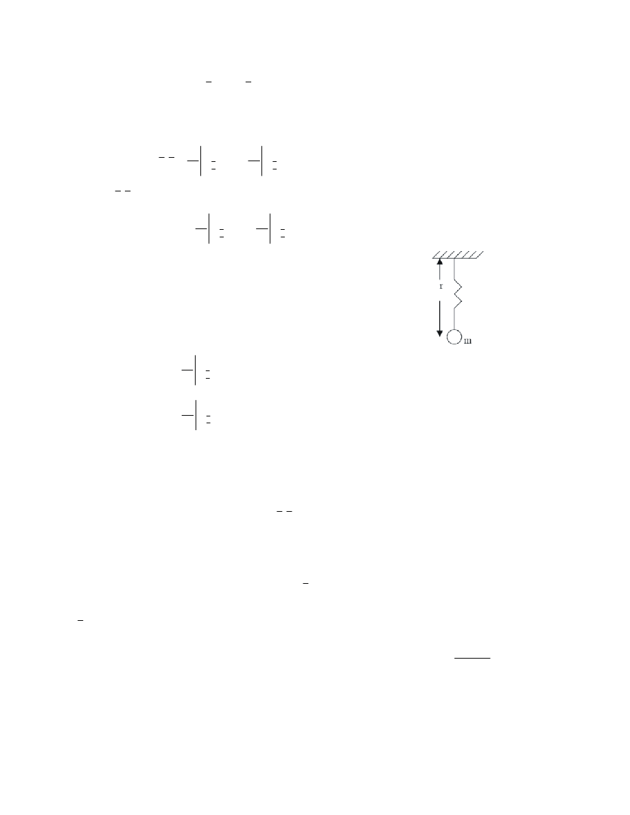
IV. EXAMPLE

Consider the system shown below.

The governing differential equations of motion for the

above system is given by

2

0

cos

0

mr

kr

kl

mr

mg

− −

=

θ −

θ =





... (1)

2

sin

0

mr

mr

mg

θ −

θ −

θ =







... (2)

where, l

0

is the initial length of the spring and ‘k’ is the

stiffness constant of the spring.

Note that the above differential equations are non-linear

in nature. First, to find the equilibrium point, equate all the
derivative terms to zero. Therefore equation (2) reduces to

mgsin

θ

= 0,

= sin

θ

= 0,

=

θ

= n

π

.

There

θ

0

= 0 is one equilibrium point for the above

system.

Following the same procedure for equation (1), we get

kr – kl

0

– mgcos

θ

= 0,

= kr – kl

0

– mg = 0,

0

0

kl

mg

r

r

k

−

= =

=

... (3)

Therefore r = r

0

is the equilibrium value for the variable

‘r’.

Expanding each term in equation (1) by Taylor's series

about the equilibrium point and neglecting the higher order
terms, we have

2

0

cos

0,

mr

kr

kl

mr

mg

− −

− θ −

θ =





Tailor and Bhathawala

0

0

0

0

0

2

0

2

2

0

0

0

0

(

)

(

)

(

)

(

)

(

0) (

cos )

(

cos )

(

0)

0,

r r

r r

r r

mr

kr

kl

mr

mr

r

r

r

mr

mg

mg

=

θ=θ

=

θ=

=

θ=

θ=θ

θ=

=

− −

−

θ

∂

−

θ

∂

∂

−

−

θ

∂θ

θ − −

θ

∂

−

θ

∂θ

θ − =











0

0

mr

kr

kl

mg

=

− −

−

=



... (4)

Following the same procedure for equation (2), we get

2

sin

0,

mr

mr

mg

θ −

θ −

θ =







0

0

0

0

0

0

0

0

0

0

0

0

0

0

0

0

0

(

)

(2

)

(

)

(

)

(

0) (2

)

(2

)

(

)

(2

)

(

0) (

sin )

(

sin )

(

0)

0

r r

r r

r r

r r

r r

r r

mr

mr

r

r

r

mr

mr

mr

r

r

r

mr

mg

mg

=

θ=θ

=

θ=

=

θ=

=

θ=θ

=

θ=

=

θ=

θ−θ

θ=

∂

=

θ

−

θ

∂

∂

−

−

θ

∂θ

θ − −

θ

∂

−

θ

∂

∂

−

−

θ

∂θ

− θ − −

θ

∂

−

θ

∂θ

θ − =



























0

0

mr

mg

θ −

θ =



... (5)

Equations (4) and (5) represent the linearized differential

equation of motion for the above system.

V. CONCLUSION

Our method is to find linear differential equation by

Taylor's series expansion and use of Jacobian linearization
process. But here find linear system only at equilibrium
points. This method is useful for check the stability of
system of differential system and stability is depends upon
the nature of the eigenvalue. This method is used for
nonlinear model.

VI. ACKNOWLEDGEMENT

The authors wish to thank the referee for his valuable

comments and suggestions.

REFERENCES

[1] Wei-Bin Zhang, "Differential equations, bifurcations, and

chaos in economics", pp. 182-185.

[2] David Betounes, "Differential equations: theory and

applications with Maple" pp. 267-268.

[3] Panos J. Antsaklis, Anthony N. Michel, "A linear systems

primer" pp. 141-143.

[4] Carmen Charles Chicone, "Ordinary differential equations

with applications" pp. 20-25.

[5] J. David Logan, "A First Course in Differential Equations"

pp. 299-301.

[6] Karl Johan Åström, Richard M. Murray "Feedback systems:

an introduction for scientists and engineers" pp. 158-161

[7] Dale E. Seborg, Thomas F. Edgar, Duncan A. Mellichamp,

Francis J. Doyle, "Process Dynamics and Control" Volume-
III, pp. 65.