8.6 Linearization of Nonlinear Systems

In this section we show how to perform linearization of systems described by

nonlinear differential equations. The procedure introduced is based on the Taylor

series expansion and on knowledge of nominal system trajectories and nominal

system inputs.

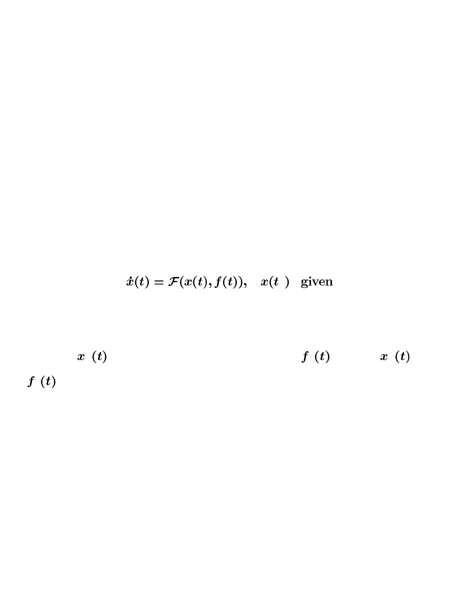
We will start with a simple scalar first-order nonlinear dynamic system

Assume that under usual working circumstances this system operates along the

trajectory

while it is driven by the system input

. We call

and

, respectively, the nominal system trajectory and the nominal system input.

The slides contain the copyrighted material from Linear Dynamic Systems and Signals, Prentice Hall 2003. Prepared by Professor Zoran Gajic

8–83

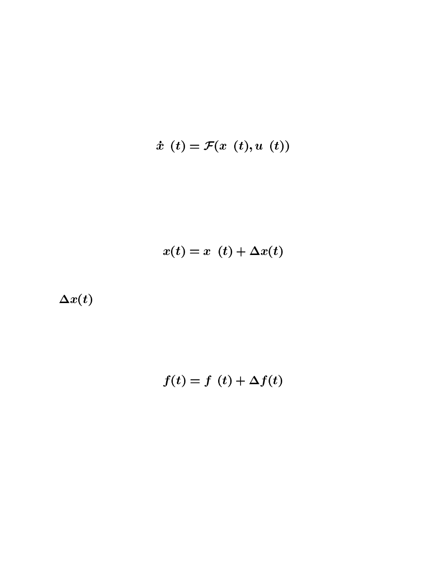
On the nominal trajectory the following differential equation is satisfied

Assume that the motion of the nonlinear system is in the neighborhood of the

nominal system trajectory, that is

where

represents a small quantity. It is natural to assume that the system

motion in close proximity to the nominal trajectory will be sustained by a system

input which is obtained by adding a small quantity to the nominal system input

The slides contain the copyrighted material from Linear Dynamic Systems and Signals, Prentice Hall 2003. Prepared by Professor Zoran Gajic

8–84

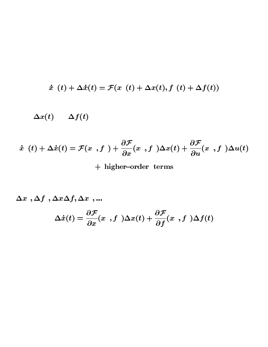
For the system motion in close proximity to the nominal trajectory, we have

Since

and

are small quantities, the right-hand side can be expanded

into a Taylor series about the nominal system trajectory and input, which produces

Canceling

higher-order

terms

(which

contain

very

small

quantities

), the linear differential equation is obtained

The slides contain the copyrighted material from Linear Dynamic Systems and Signals, Prentice Hall 2003. Prepared by Professor Zoran Gajic

8–85

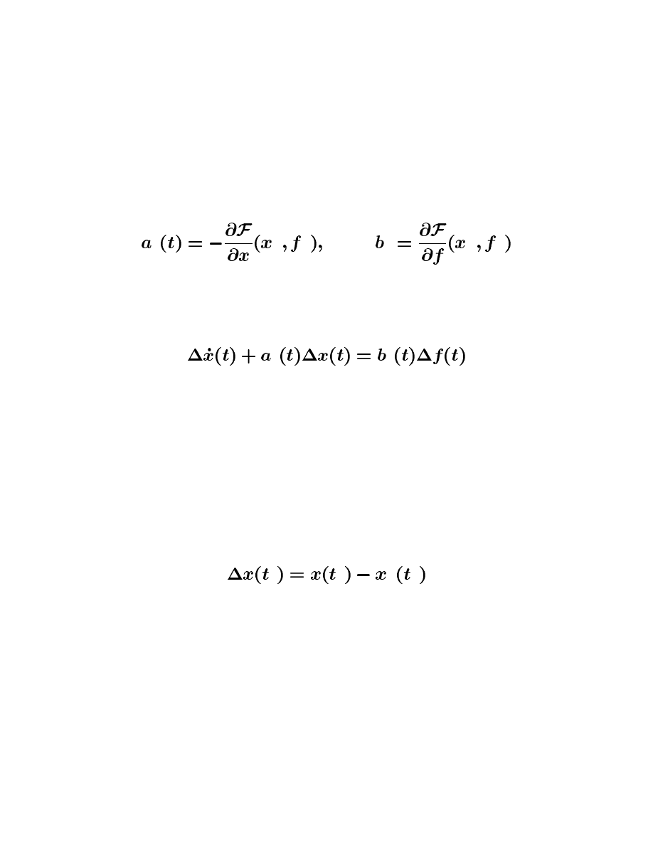
The partial derivatives in the linearization procedure are evaluated at the nominal

points. Introducing the notation

the linearized system can be represented as

In general, the obtained linear system is time varying. Since in this course we

study only time invariant systems, we will consider only those examples for which

the linearization procedure produces time invariant systems. It remains to find the

initial condition for the linearized system, which can be obtained from

The slides contain the copyrighted material from Linear Dynamic Systems and Signals, Prentice Hall 2003. Prepared by Professor Zoran Gajic

8–86

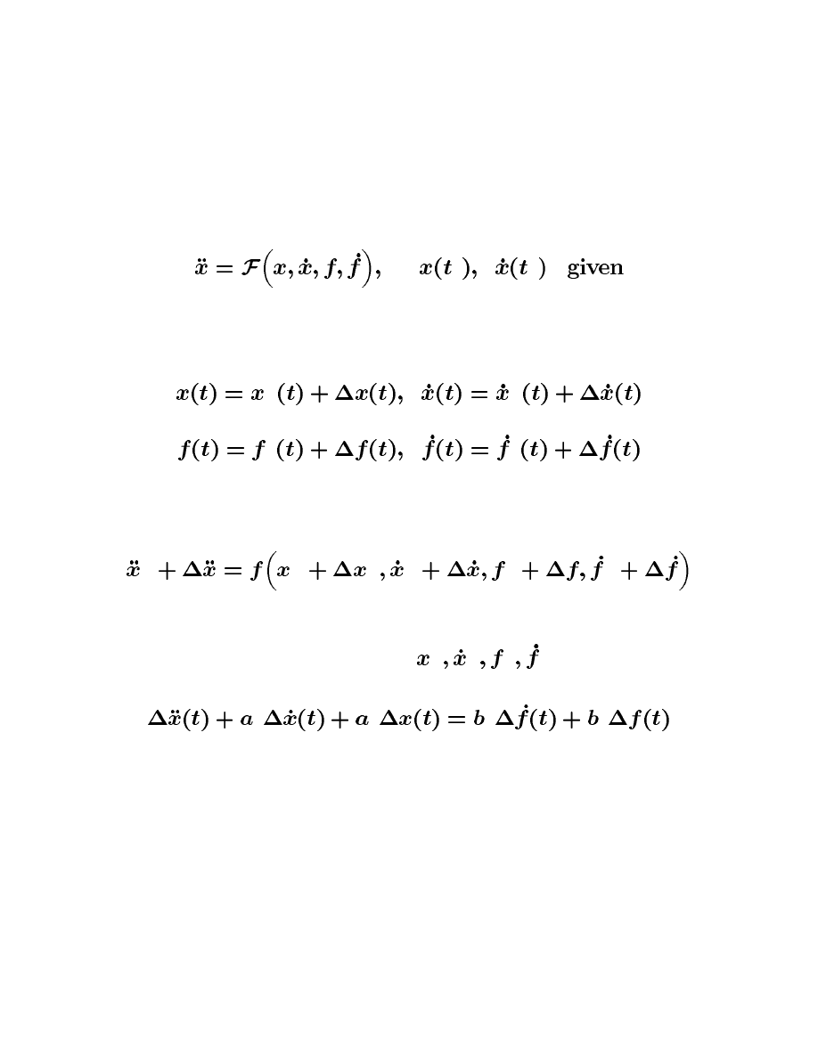
Similarly, we can linearize the second-order nonlinear dynamic system

by assuming that

and expanding

into a Taylor series about nominal points

, which leads to

The slides contain the copyrighted material from Linear Dynamic Systems and Signals, Prentice Hall 2003. Prepared by Professor Zoran Gajic

8–87

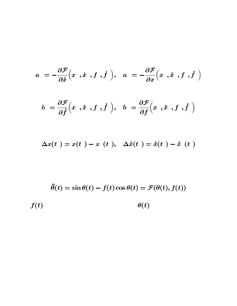
where the corresponding coefficients are evaluated at the nominal points as

The initial conditions for the second-order linearized system are obtained from

Example 8.15: The mathematical model of a stick-balancing problem is

where

is the horizontal force of a finger and

represents the stick’s angular

displacement from the vertical.

The slides contain the copyrighted material from Linear Dynamic Systems and Signals, Prentice Hall 2003. Prepared by Professor Zoran Gajic

8–88

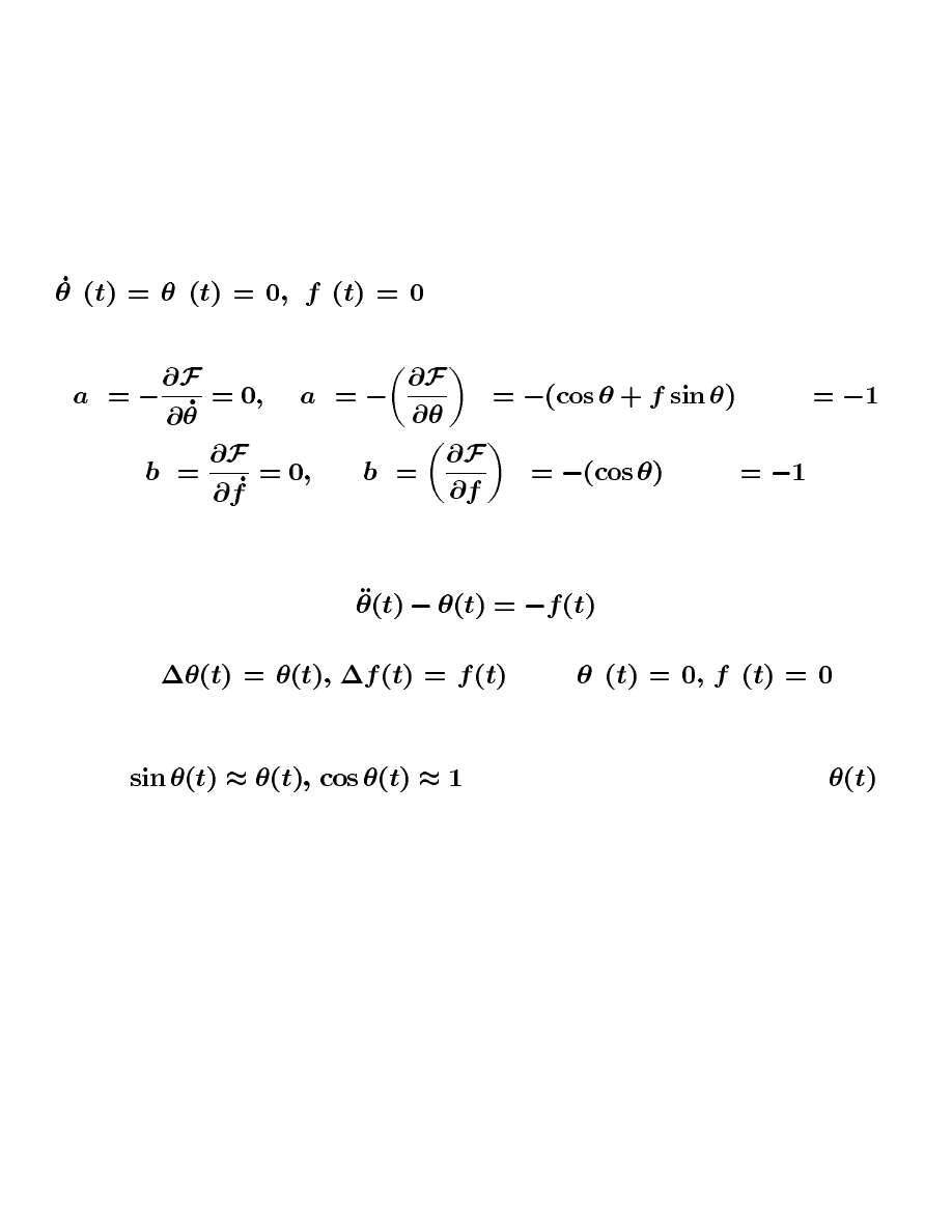
This second-order dynamic system is linearized at the nominal points

, producing

!"

The linearized equation is given by

Note that

since

. It is

important to point out that the same linearized model could have been obtained by

setting

, which is valid for small values of

.

The slides contain the copyrighted material from Linear Dynamic Systems and Signals, Prentice Hall 2003. Prepared by Professor Zoran Gajic

8–89

We can extend the presented linearization procedure to an

-order nonlinear

dynamic system with one input and one output in a straightforward way. However,

for multi-input multi-output systems this procedure becomes cumbersome. Using

the state space model, the linearization procedure for the multi-input multi-output

case is simplified.

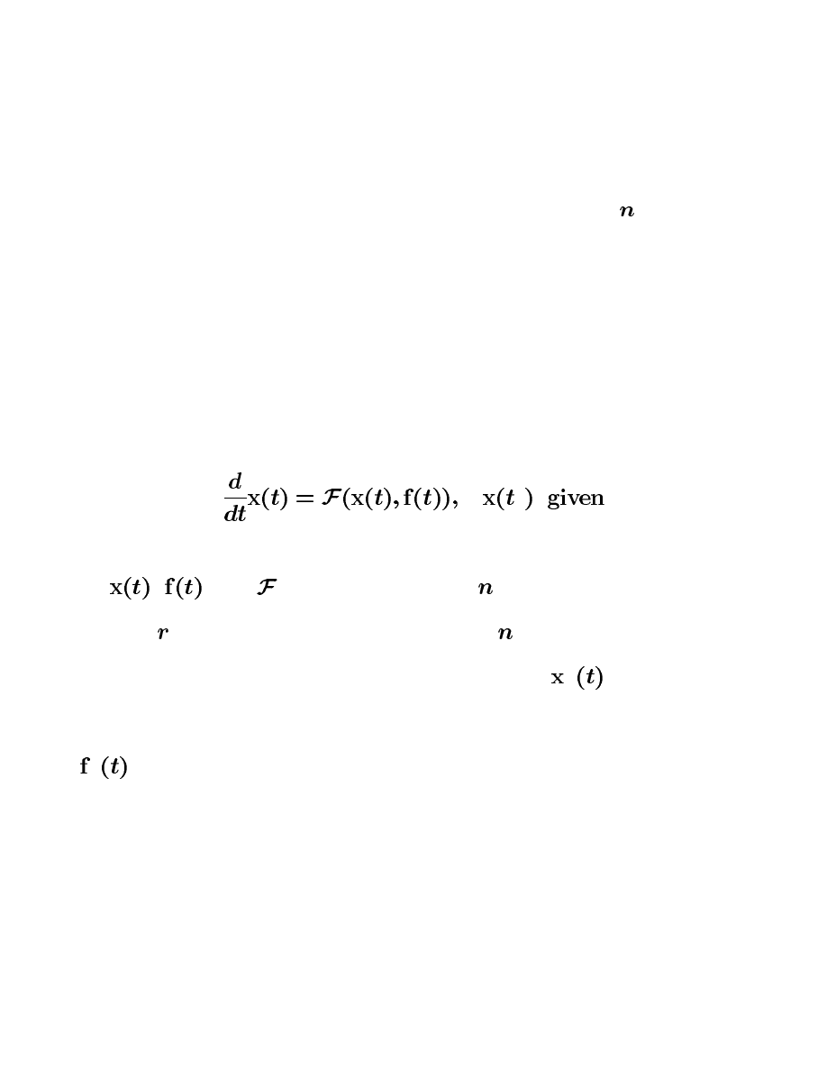
Consider now the general nonlinear dynamic control system in matrix form

#

where

,

, and

are, respectively, the

-dimensional system state space

vector, the

-dimensional input vector, and the

-dimensional vector function.

Assume that the nominal (operating) system trajectory

$

is known and that

the nominal system input that keeps the system on the nominal trajectory is given

by

$

.

The slides contain the copyrighted material from Linear Dynamic Systems and Signals, Prentice Hall 2003. Prepared by Professor Zoran Gajic

8–90

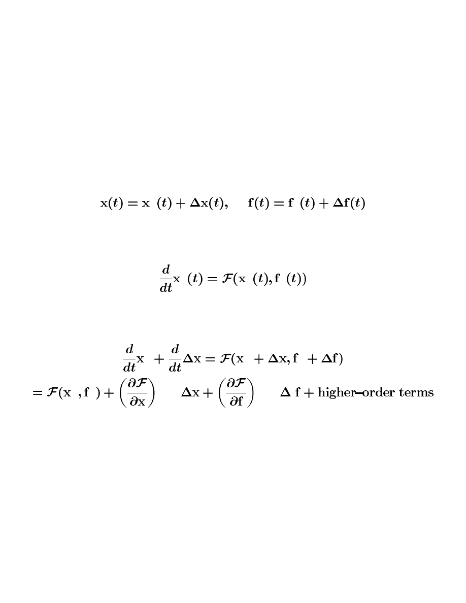
Using the same logic as for the scalar case, we can assume that the actual

system dynamics in the immediate proximity of the system nominal trajectories can

be approximated by the first terms of the Taylor series. That is, starting with

%

%

and

%

%

%

we expand the right-hand side into the Taylor series as follows

%

%

%

%

%

&"')(+*,-

.

(

*/,-

&'0(1*,-

.

(

*,-

The slides contain the copyrighted material from Linear Dynamic Systems and Signals, Prentice Hall 2003. Prepared by Professor Zoran Gajic

8–91

Higher-order terms contain at least quadratic quantities of

and

. Since

and

are small their squares are even smaller, and hence the high-order terms

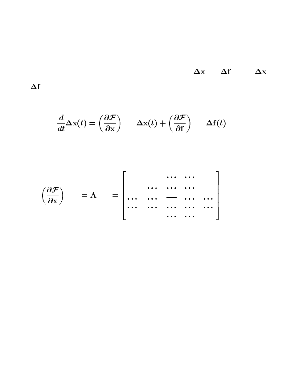
can be neglected. Neglecting higher-order terms, an approximation is obtained

2"3541678

9

4

678

2354:6;78

9

4

678

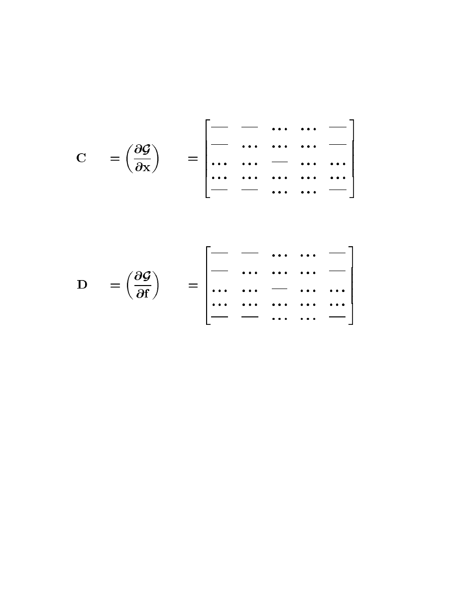
The partial derivatives represent the Jacobian matrices given by

2"3546!78

9

4

6;78

<>=?<

@BADC

@FE

C

@BADC

@FEBG

@HAIC

@FE

4

@BA

G

@FE

C

@HA

G

@FE

4

@HAKJ

@FEML

@HA

4

@FE

C

@HA

4

@FEBG

@BA

4

@FE

4

23

4

678

9

4+678

The slides contain the copyrighted material from Linear Dynamic Systems and Signals, Prentice Hall 2003. Prepared by Professor Zoran Gajic

8–92

NO5PQRS

T

PQRS

U>V?W

XFY[Z

X]\

Z

XHYIZ

X^\`_

XHYIZ

X^\ba

XHY

_

X^\`Z

XHY

_

X^\

a

XHYKc

Xd\fe

XHY

P

X^\

Z

XHY

P

X^\

_

XHY

P

X^\

a

N

O

P

Q!RS

T

P

Q!RS

Note that the Jacobian matrices have to be evaluated at the nominal points, that

is, at

U

and

U

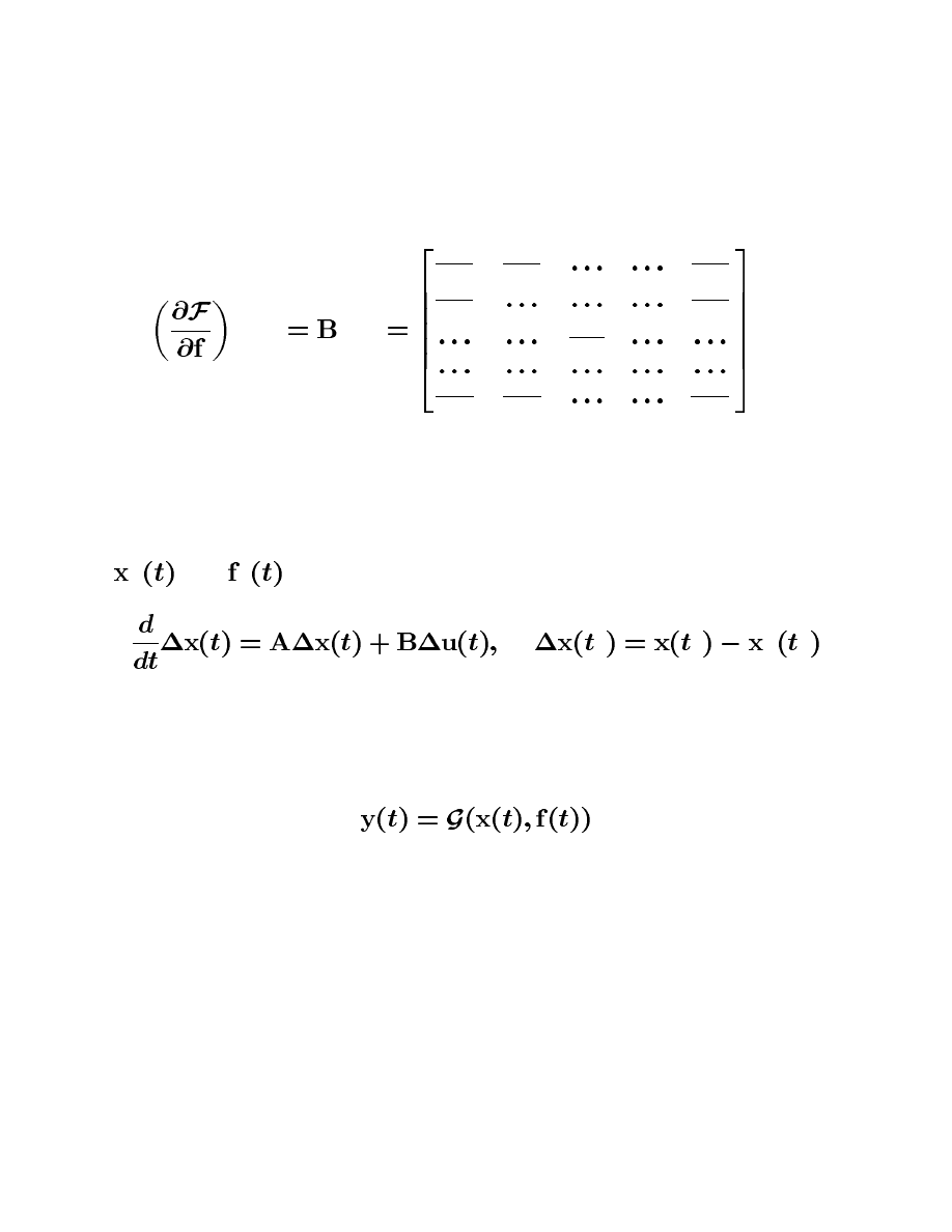
. With this notation, the linearized system has the form

g

g

U

g

The output of a nonlinear system satisfies a nonlinear algebraic equation, that is

The slides contain the copyrighted material from Linear Dynamic Systems and Signals, Prentice Hall 2003. Prepared by Professor Zoran Gajic

8–93

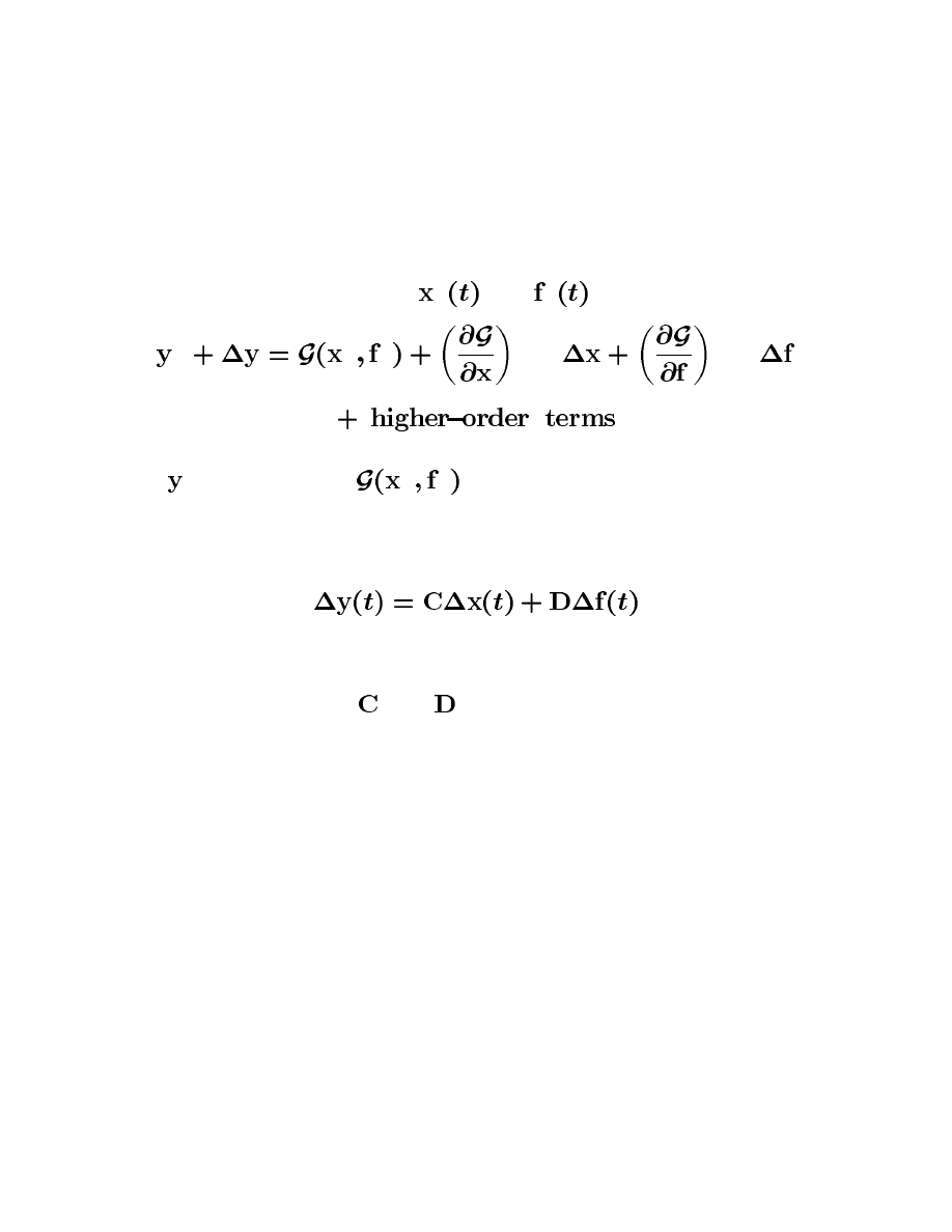
This equation can also be linearized by expanding its right-hand side into a

Taylor series about nominal points

h

and

h

. This leads to

h

h

h

i"j5kl!mn

o

k

l!mn

i"j5k+l;mn

o

k

l!mn

Note that

h

cancels term

h

h

.

By neglecting higher-order terms, the

linearized part of the output equation is given by

where the Jacobian matrices

and

satisfy

The slides contain the copyrighted material from Linear Dynamic Systems and Signals, Prentice Hall 2003. Prepared by Professor Zoran Gajic

8–94

prqts

u"v)w:x;yz

{

wxyz

|F}^~

|

~

|}d~

|FB€

|}d~

|

w

|F}

€

|

~

|}

€

|

w

|F}B

|F:‚

|}ƒ

|FF~

|}:ƒ

|F

€

|}:ƒ

|

w

u

v

w

x;yz

{

w

x;yz

prq…„

u"v

w

xyz

{

w

xyz

|}

~

|^†

~

|F}

~

|d†

€

|F}

~

|d†ˆ‡

|}F€

|^†‰~

|F}€

|d†

‡

|}



|^†

‚

|}

ƒ

|^†

~

|F}

ƒ

|d†ˆ€

|F}

ƒ

|^†

uv

w

xyz

{

w

xyz

The slides contain the copyrighted material from Linear Dynamic Systems and Signals, Prentice Hall 2003. Prepared by Professor Zoran Gajic

8–95

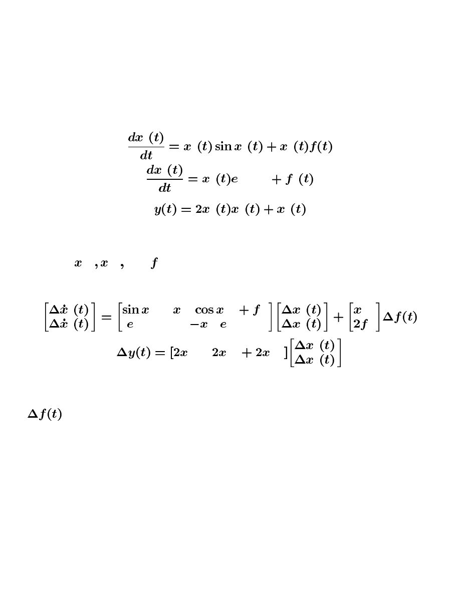
Example 8.16: Let a nonlinear system be represented by

Š

Š

‹

‹

‹

Š

ŒKBŽb‘5’

‹

Š

‹

‹

‹

Assume that the values for the system nominal trajectories and input are known and

given by

Šf“

‹ˆ“

and

“

. The linearized state space equation of this nonlinear

system is obtained as

Š

‹

‹ˆ“

Šf“

‹b“

“

Œ[

Ž•”

Šf“

Œ[

Ž–”

Š

‹

‹ˆ“

“

‹ˆ“

Šf“

‹ˆ“

Š

‹

Having obtained the solution of this linearized system under the given system input

, the corresponding approximation of the nonlinear system trajectories is

The slides contain the copyrighted material from Linear Dynamic Systems and Signals, Prentice Hall 2003. Prepared by Professor Zoran Gajic

8–96

—

˜

—

™

—

˜

™

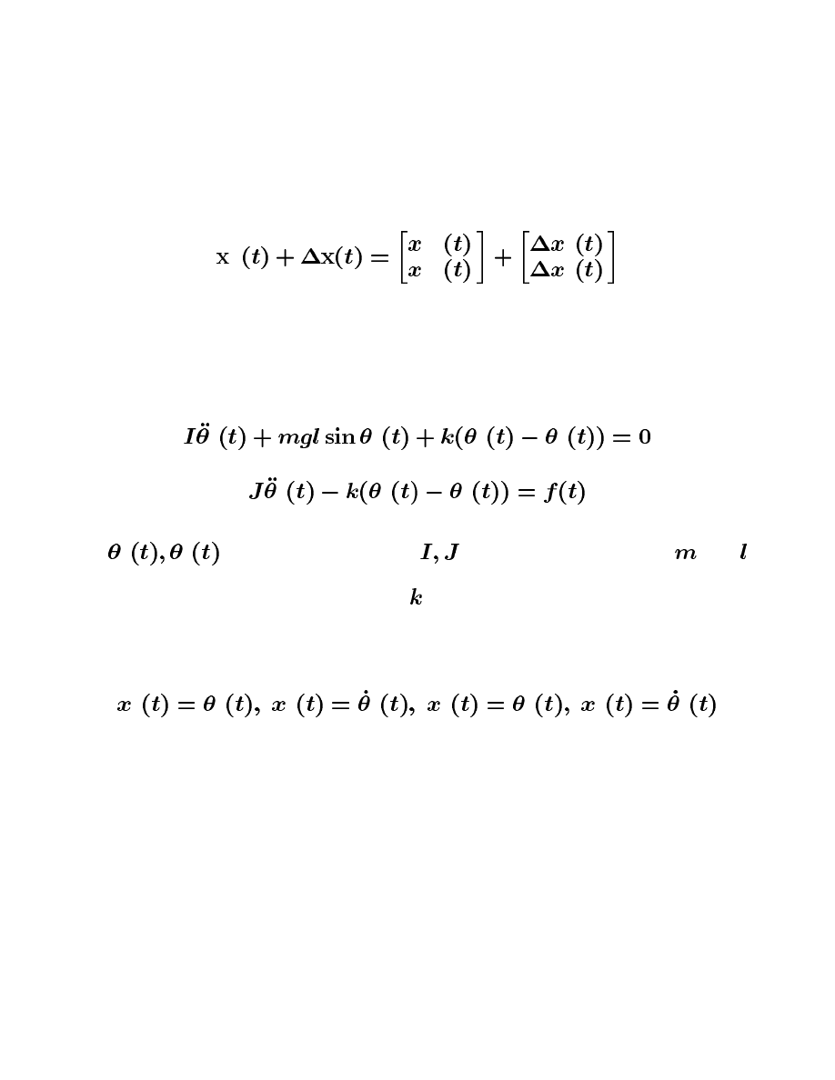
Example 8.17: Consider the mathematical model of a single-link robotic ma-

nipulator with a flexible joint given by

˜

˜

˜

™

™

˜

™

where

˜

™

are angular positions,

are moments of inertia,

and are,

respectively, link mass and length, and

is the link spring constant. Introducing

the change of variables as

˜

˜

™

˜

š

™

›

™

the manipulator’s state space nonlinear model is given by

The slides contain the copyrighted material from Linear Dynamic Systems and Signals, Prentice Hall 2003. Prepared by Professor Zoran Gajic

8–97

œ





œ

œ

ž

ž

Ÿ

Ÿ

œ

ž

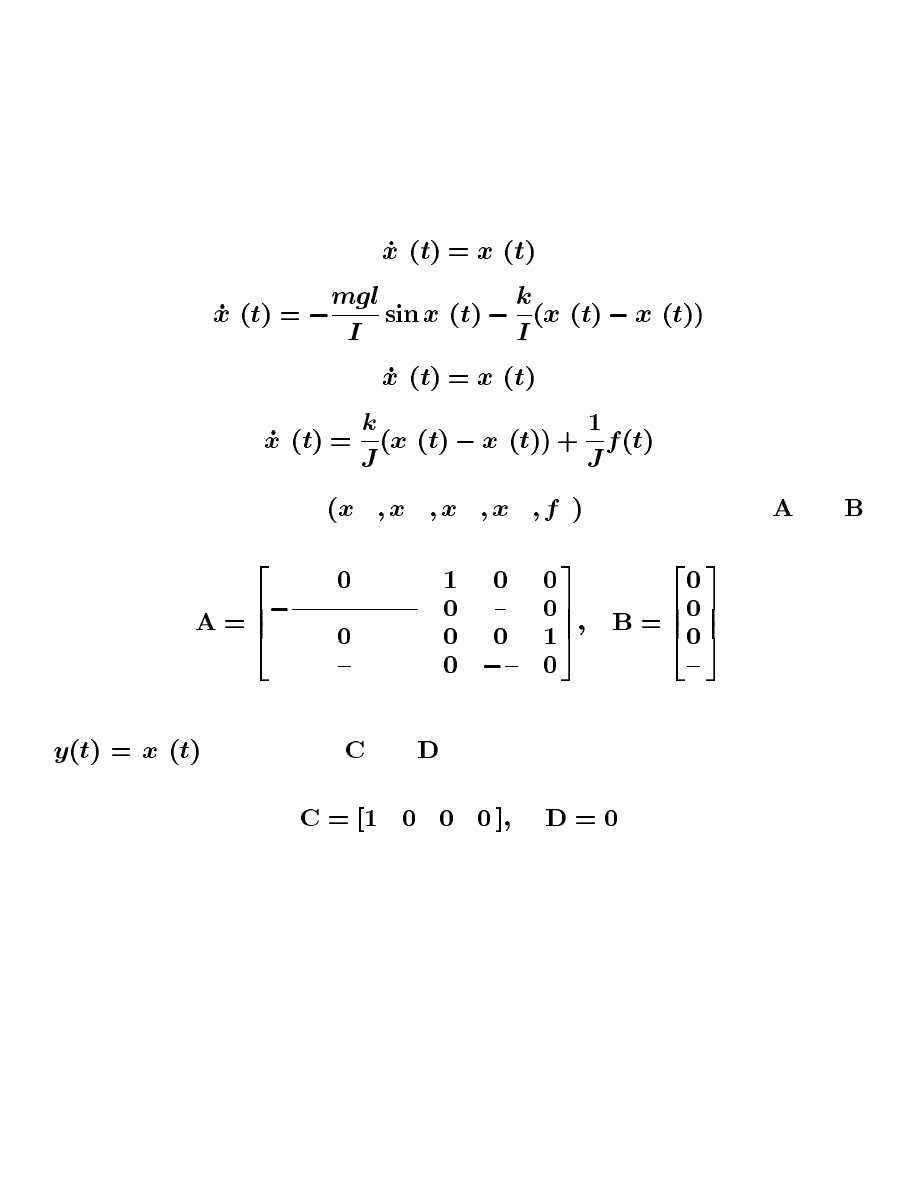
Take the nominal points as

œf 

b 

ž` 

Ÿ` 

 

, then the matrices

and

are

¡:¢¤£¦¥+§©¨«ª`¬+­F®°¯

±

¡

±

¡

²

¡

²

œ

²

Assuming that the output variable is equal to the link’s angular position, that is

œ

, the matrices

and

are given by

The slides contain the copyrighted material from Linear Dynamic Systems and Signals, Prentice Hall 2003. Prepared by Professor Zoran Gajic

8–98