BULLETIN OF THE POLISH ACADEMY OF SCIENCES
TECHNICAL SCIENCES
Vol. 54, No. 1, 2006

Linearization of non-linear state equation

A.J. JORDAN

∗

Faculty of Electrical Engineering, Bialystok Technical University, 45D Wiejska St., 15-351 Bialystok, Poland

Abstract. The paper presents an overview of linearization methods of the non-linear state equation. The linearization is developed from the
point of view of the application in the theoretical electrotechnics. Some aspects of these considerations can be used in the control theory.
In particular the main emphasis is laid on three methods of linearization, i.e.: Taylor’s series expansion, optimal linearization method and
global linearization method. The theoretical investigations are illustrated using the non-linear circuit composed of a solar generator and a DC
motor. Finally, the global linearization method is presented using several examples, i.e. the asynchronous slip-ring motor and non-linear diode.
Furthermore the principal theorem concerning the BIBS stability (bounded-input bounded state) is introduced.

Key words: non-linear state equation, linearization, optimal linearization method, global linearization method, Taylor’s series expansion, BIBS
stability.

1. Introduction

The subject of the linearization of nonlinear state equation has
been discussed in a number of papers concerning theoretical
electrotechnics and control theory [1–8]. This problem in-
volves ranges of equivalence of the linear model both in di-
rect mapping of the systems dynamics as well as their stability,
controllability and observability [2,5,9]. The most common
linearization method i.e. expansion in Taylor’s series around
the equilibrium point is a very effective approximation of the
non-linear model only for some minor deviation of state vari-
ables from the equilibrium point [4]. However, this method
can be a good starting point for other methods that are good
approximations in the whole state space [4,10,11]. In recent
years a significant importance has had the linearization by vari-
able transformation which is based on global diffeomorphism
[6–8]. Its fundamental principles will be presented in a fur-
ther part of this paper. It should be noted, however, that the
continuity of the non-linear functions and their differentiabil-
ity plays, in this case, the most significant role [6,7,12]. An
interesting method of linearization was presented in paper [9],
where non-linear state equation was approximated by linear
state model with matrix A = A(t). In this case the sequence
of linear observers is uniformly convergent which results in an
observer for a non-linear system. In paper [13] the scalar non-
linear Bernoulli equation was also approximated by the linear
model and it was found that there was a good agreement of the
approximation series ˙

x = A[x(t)

n

]x, (n = 1, 2, ...) with the

numerical solution of the non-linear equation ˙

x = f (x, t). The

linearization of the multi-input, multi-output systems (MIMO)
by the input-output injection was presented in papers [3,14,15].
Works [6,7] present little known Frobenius theorem concern-
ing the linearization of partial differential equations. More-
over, it should be stressed that Frobenius integrability of cer-
tain distributions associated to a control system is equivalent
to its feedback linearizability. It should be also noted that a

historical review of non-linear control methods, which also de-
scribes the linearization of non-linear systems, is presented in
paper [16].

In this work in overview of the basic methods of the

linearization of non-linear state equation is presented. The
overview concerns basic problems of theoretical electrotech-
nics dealing with the linearization of the non-linear state equa-
tions. The problems presented here can be also used in control
theory.

In many considerations concerning system dynamics the

physical systems are treated as linear systems.

This fol-

lows from assumed simplified statements that say that the
characteristics of system elements are linear in character, or
that the equation linearized by Taylor’s expansion occurs for
some small deviations of state variables around the equilib-
rium point. However, in many cases, it is impossible to accept
such assumptions and for our analysis we assume the following
system of non-linear equations.

˙x = f (x, u, t),

x(0) = x

0

(1)

where f (x, u, t) is the vector of nonlinear functions, x(t) ∈
R

n

and u(t) ∈ R

m

are the vector of the state variables and

the input vector, respectively; x

0

represents the set of initial

conditions.

In practical considerations, to solve Eq. (1) we apply the

numerical methods [17–20]. The problems of the solution of
Eq. (1) are not examined exactly. Alike, the stability of the sys-
tem that is described by Eq. (1) is the open problem [21,22].

For this reason, we approximate the Eq. (1) by linear state

equation

˙x(t) = Ax(t) + Bu(t),

x(0) = x

0

.

(2)

The form of the matrices A and B depends of the method

of the linearization of Eq. (1). Equation (2) has the analytical

∗

e-mail: [e-mail]

63

A.J. Jordan

solution

x(t) = e

A(t−t

0

)

x

0

+

t

Z

t

0

e

A(t−τ )

Bu(τ )dt.

(3)

Assuming t

0

= 0, w obtain

x(t) = e

At

x

0

+

t

Z

0

e

A(t−τ )

Bu(τ )dt.

(4)

The exact solution of Eq. (2) resulting from Eq. (3) or Eq. (4)
is very important to solve the stability problems in the linear
systems. However, in practice, for the number of state vari-
ables n > 3 we use the numerical methods to compute the
vector x(t).

The homogeneous state equation is given as follows

˙x(t) = Ax(t),

x(0) = x

0

.

(5)

The solution of (5) takes the form

x(t) = e

A(t−t

0

)

x

0

(6)

or

x(t) = e

At

x

0

,

if

t

0

= 0.

(7)

T

HEOREM

1. The system described by homogeneous Eq.

(5) is asymptotically stable if and only if the eigenvalues of
matrix A have the negative real parts [22].

In the case of the non-homogenous equation, we can for-

mulate the following theorem:

T

HEOREM

2. The system described by non-homogenous

Eq. (2) with input u(t) is BIBS (bounded-input bounded state)
stable if and only if the eigenvalues of matrix A have the neg-
ative real parts and the input u(t) is limited [8].

This theorem is equitable in the case, where we do not meet

the secular terms [23].

The linearization of non-linear state equation (1) aims to

make the linear approach (2) a good approximation of the non-
linear equation in the whole state space and for time t → ∞.
In the above case the linear approach can ensure the existence
and an unambiguous solution for the non-linear equation. It
can also constitute a mathematical model that makes it possi-
ble to investigate the stability of the non-linear system.

In this paper three linearization methods of the non-linear

state equation are defined:
– expansion in Taylor’s series,
– optimal linearization method,
– global linearization method.

The problem of the linearization based on the geometrical

approach will be discussed in another paper.

To illustrate the above linearization methods we use the

same non-linear electric circuit containing a DC motor sup-
plied by a solar generator.

2. Non-linear electric circuit with a DC motor

supplied by a solar generator

To illustrate the theoretical results developed for the three
methods mentioned above, the non-linear electrical circuit with

the solar generator and DC drive system is analysed. The non-
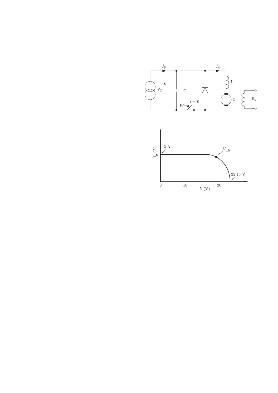
linear circuit is presented in Fig. 1. In the time t = 0 the switch
W is closed and the circuit is in a transient state. The non-
linear characteristic of the solar generator is showed in Fig. 2
[24,25].

Fig. 1. An electric circuit containing a solar generator and a DC motor

Fig. 2. Non-linear characteristic of solar generator. V

p,0

= 22, 15 V

is the generator voltage prior to switching on switch W . V

p,b

is the

equilibrium point of the system (steady state)

The transient state of the circuit is described by the follow-

ing set of equations [24,25].

˙x

1

= −a

1

e

ax

1

− a

2

x

2

+ u

˙x

2

= a

3

x

1

− a

4

x

2

− a

5

x

3

˙x

3

= a

6

x

2

− a

7

x

3

;

x

1

(0) = V

p,0

,

x

2

(0) = 0,

x

3

(0) = 0,

(8)

where x

1

= V

p

is the generator voltage, x

2

= I

M

is the rotor

current and x

3

= Ω represents the DC motor rotational speed.

The non-linear characteristic of the solar generator is approxi-
mated using the following formula

I

p

= I

0

− I

s

(e

aV

p

− 1).

(9)

In this formula I

0

is the photovoltaic current of the cell

(V

p

= 0) dependent on light flux, I

s

is the saturation current

defined by Shockley equation, whereas a is the factor that char-
acterizes the solar generator.

The coefficients a

1

, ..., a

7

and u are expressed by the rela-

tions that combine the parameters of non-linear circuit (Figs. 1
and 2)

a

1

=

I

s

C

,

a

2

=

1

C

,

a

3

=

1

L

,

a

4

=

R

m

L

a

5

=

K

x

L

,

a

6

=

K

x

J

,

a

7

=

K

r

J

,

u =

I

0

+ I

s

C

.

(10)

64

Bull. Pol. Ac.: Tech. 54(1) 2006

Linearization of non-linear state equation

In the numerical computations, we use the following values of
the parameters:

R

m

= 12.045 Ω,

L = 0.1 H,

C = 500µF,

K

x

= 0.5 Vs,

K

r

= 0.1 Vs

2

,

J = 10

−3

Ws

3

,

I

0

= 2 A,

I

s

= 1.28 · 10

−3

A,

a = 0.54 V

−1

,

V

p,0

= 22.15 V.

(11)

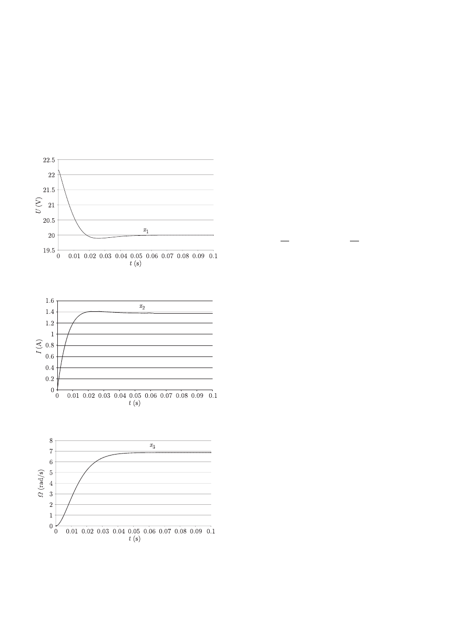
The system of non-linear Eqs. (8) is solved using Runge-Kutta
method [20] with the integration step h = 10

−6

s. The solution

is presented in Figs. 3, 4 and 5.

Fig. 3. The diagram of state variable x

1

Fig. 4. The diagram of state variable x

2

Fig. 5. The diagram of state variable x

3

3. Expansion in the Taylor’s series

Let x

eq

, u

eq

be the equilibrium point of the system (1), i.e.

˙x

eq

= f (x

eq

, u

eq

, t)

(12)

and

∆x = x − x

eq

,

∆u = u − u

eq

(13)

are the small differences for the state vector and the input vec-
tor, respectively. Assuming that

∆ ˙x = ˙x − ˙x

eq

= ˙x − f (x

eq

, u

eq

, t)

(14)

and expanding in Taylor’s series the right side of Eq. (1), and
neglecting the terms of order higher than first, we obtain the
approximation of this equation in the form of the following
linear equation

∆ ˙x = A∆x + B∆u.

(15)

We usually write Eq. (15) in the form [4,26]

˙x(t) = Ax(t) + Bu(t)

(16)

where

A =

∂f
∂x

¯

¯

¯

¯

x=x

eq

u=u

eq

,

B =

∂f
∂u

¯

¯

¯

¯

x=x

eq

u=u

eq

.

(17)

Now, we consider the electric circuit presented in Fig. 1.

To simplify the linearization of the equation system (8) in Eq.
(16) we use transient and steady components in our analysis

x(t) = x

s

(t) + x

t

(t).

(18)

The steady components x

s

(t) are computed from the set of

non-linear algebraic equations

f (x

s

(t), u

s

(t)) = 0

(19)

and the transient components x

t

(t) are the solution of homo-

geneous equations

˙x

t

− ˙x

eq

= A(x

t

− x

eq

).

(20)

For the stable system we have ˙

x

eq

= x

eq

= 0 and Eq. (20) is

reduced to

˙x

t

= Ax

t

(t),

x

t

(0) = x(0) − x

s

(0)

(21)

where matrix A is computed using both Eq. (17) and constant
x = x

eq

= x

s

, u = u

eq

. To illustrate this method we use

the example described in Section 2. In this case the non-linear
circuit is composed with the solar generator and DC motor.

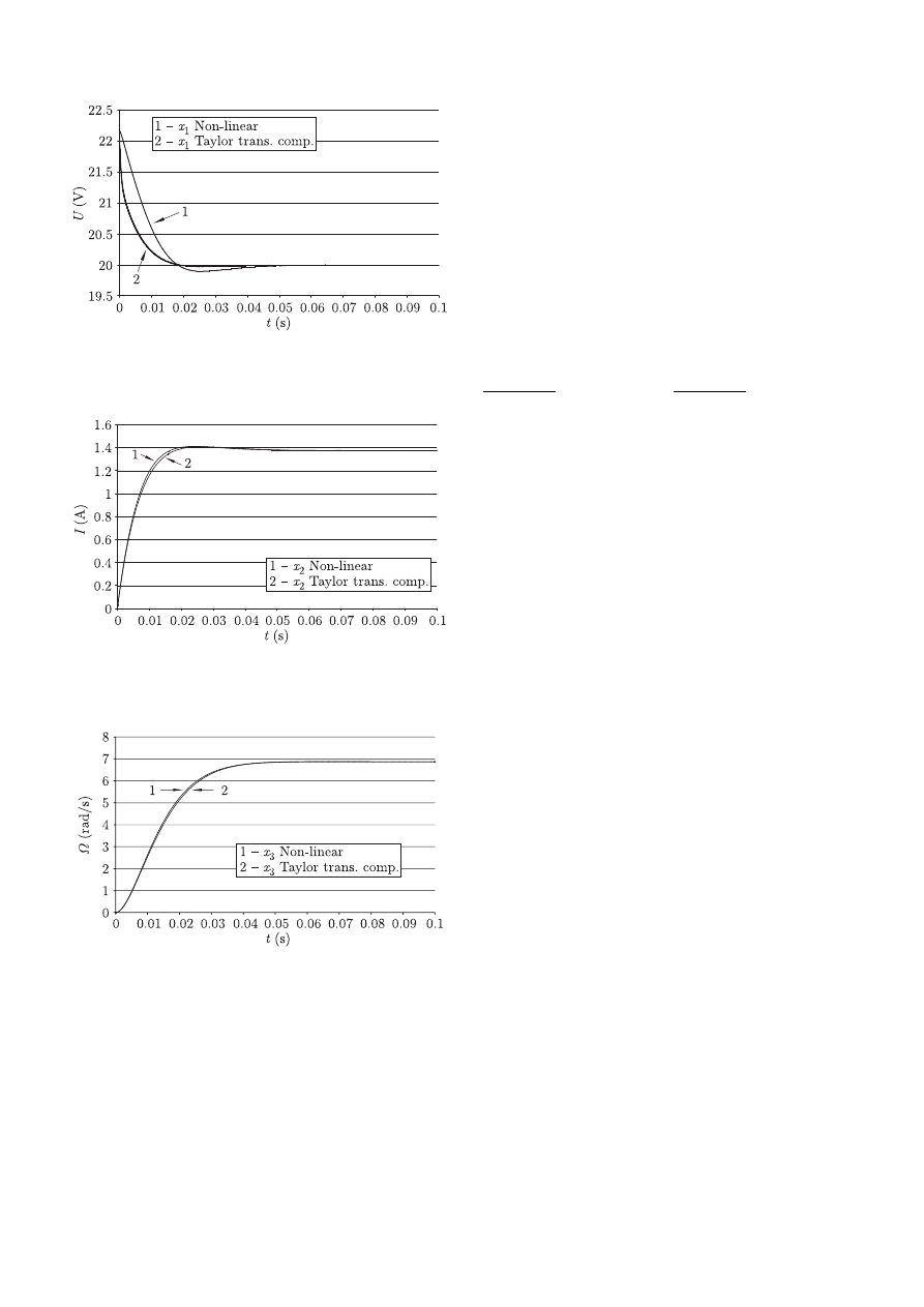
The solutions of the non-linear equation using Runge-

Kutta method with the integration step h = 10

−6

s and the

solution of linear equation (16) are represented in Figs. 6–
8. In this case we use the method of decomposition of the
state variables on the steady components x

s

(t) and transient

components x

t

(t), (x(t) = x

s

(t) + x

t

(t)). The equilibrium

point is chosen in the steady state, i.e. in the point where
f (x

s

(t), u

s

(t), t) = 0. This behaviour is named Taylor’s series

expansion around equilibrium point with the transient compo-
nents.

It is possible to realize the expansion in Taylor’s series

around the initial condition x(0) = x

0

. This procedure gives

us immediately x

eq

= x

0

and ˙

x

eq

= ˙x(t = 0). This behaviour

is very convenient for the case x

0

= 0.

Bull. Pol. Ac.: Tech. 54(1) 2006

65

A.J. Jordan

Fig. 6. The diagram of state variable x

1

– comparison between solu-

tion of non-linear Eq. (8) and solution of linear Eq. (16)

Fig. 7. The diagram of state variable x

2

– comparison between solu-

tion of non-linear equation (8) and solution of linear Eq. (16)

Fig. 8. The diagram of state variable x

3

– comparison between solu-

tion of non-linear equation (8) and solution of linear Eq. (16)

4. Optimal linearization method

The least square method makes it possible to find the method
of linearization of Eq. (1) named the optimal linearization
method [4,25,27]. In this case the non-linear equation is ap-
proximated by the optimal equation

˙x(t) = A

∗

x(t) + B

∗

u(t),

x(0) = x

0

.

(22)

The optimal matrices A

∗

and B

∗

are defined in the following

way: the small difference

ε = Ax(t) + Bu(t) − f (x(t), u(t), t)

(23)

between the right side of linear and non-linear equation is thus
defined.

Unknown elements a

∗

ij

and b

∗

ij

(i, j = 1, 2, ..., n) of the

matrices A

∗

and B

∗

are determined by minimizing of the func-

tional

I(a

ij

, b

ij

) =

t

1

Z

0

ε

T

(t)ε(t)dt

(24)

∂I(a

ij

, b

ij

)

∂a

ij

¯

¯

¯

¯ a

ij

= a

∗

ij

= 0 ,

∂I(a

ij

, b

ij

)

∂b

ij

¯

¯

¯

¯ b

ij

= b

∗

ij

= 0 .

(25)

To determine the optimal elements a

∗

ij

and b

∗

ij

, we introduce

the basis functions into the formula (23). The basis functions
can be defined using Taylor’s series expansion of the non-linear
equation (1). The time t

1

is chosen on the basis of the steady

state of the non-linear system and the integrals (24) are deter-
mined by numerical calculations.

The formulas (25) represent the necessary conditions of

optimization, and in practical applications the results received
do not require the Hesse-Matrix computations.

To linearize the non-linear systems (1) we used the follow-

ing basis functions:

– Taylor’s series expansion around equilibrium point
– Taylor’s series expansion around equilibrium point with

the transient components.

In this case two different optimal equations were obtained.
The optimal matrices A

∗

1

and A

∗

2

with the numerical values

of elements taken from the example presented in section 2,
are shown below (A

∗

1

represents the case of Taylor’s series ex-

pansion around equilibrium point, and A

∗

2

represents the case

of Taylor’s series expansion around equilibrium point with the
transient components).

A

∗

1

=





−1466.31 −1919.04 −20.5118

10

−120.45

−5

0

500

−100





A

∗

2

=





−1457.07 −2447.53 −15.8207

10

−120.45

−5

0

500

−100



 .

Matrix B

∗

is the same for both cases:

B

∗

=

£

1 0 0

¤

T

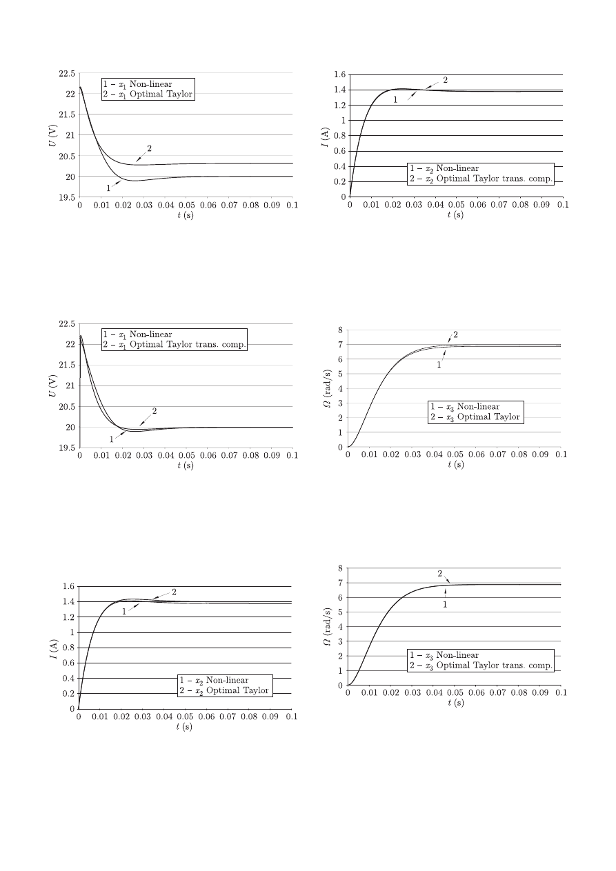
The results of computations are presented in Figs. 9–14.

It is necessary to point out that the good results of the lin-

earization of non-linear equation with the Taylor’s expansion
around equilibrium point with the transient components are ob-
tained.

66

Bull. Pol. Ac.: Tech. 54(1) 2006

Linearization of non-linear state equation

Fig. 9. The diagram of state variable x

1

– comparison between solu-

tion of non-linear equation (8) and solution of optimal Eq. (22) based

on Taylor’s series expansion around the equilibrium point

Fig. 10. The diagram of state variable x

1

– comparison between so-

lution of non-linear Eq. (8) and solution of optimal Eq. (22) based
on Taylor’s series expansion around the equilibrium point with the

transient components

Fig. 11. The diagram of state variable x

2

– comparison between so-

lution of non-linear Eq. (8) and solution of optimal Eq. (22) based on

Taylor’s series expansion around the equilibrium point

Fig. 12. The diagram of state variable x

2

– comparison between so-

lution of non-linear Eq. (8) and solution of optimal Eq. (22) based
on Taylor’s series expansion around the equilibrium point with the

transient components

Fig. 13. The diagram of state variable x

3

– comparison between so-

lution of non-linear Eq. (8) and solution of optimal Eq. (22) based on

Taylor’s series expansion around the equilibrium point

Fig. 14. The diagram of state variable x

3

– comparison between so-

lution of non-linear Eq. (8) and solution of optimal Eq. (22) based
on Taylor’s series expansion around the equilibrium point with the

transient components

Bull. Pol. Ac.: Tech. 54(1) 2006

67

A.J. Jordan

5. Global linearization method

5.1. Variables transformation.

In several cases, a non-

linear equation (1) can be linearized by means of the state
variables transformation that is defined using a global diffeo-
morphism [6–8,28]. Assuming that f (x, u, t) is the continu-
ous function and n-time differentiable, we apply the following
variables transformation.

z = φ(x)

(26)

where

φ(x) =









Φ

1

(x

1

, x

2

, ..., x

n

)

Φ

2

(x

1

, x

2

, ..., x

n

)

.....................

Φ

n

(x

1

, x

2

, ..., x

n

)







 .

(27)

In this case Eq. (1) is transformed into the linear equation

˙z = Az + Bv,

z (0) = Φ [x (t = 0)]

(28)

where v is a new input v = u + f (x) and f (x) is a non-linear
combination of state variables x

1

, x

2

, ..., x

n

. The solution of

linear equation (28) is known:

z = e

At

z(0) +

t

Z

0

e

A(t−τ )

Bv(τ )dτ .

(29)

Using the inverse transformation

x = φ

−1

(z)

(30)

we obtain vector ˜

x(t) that satisfies relation ˜

x(t) ∼

= x(t) over

the whole state space where t → ∞ and x(t) is the solution of
Eq. (1). The vector ˜

x(t) results from the formula (30) and is

computed using the iterative method which is presented in the
next section.

5.2. Example of computations. We consider once more the
same example presented in Figs. 1 and 2

˙x

1

= −a

1

e

ax

1

− a

2

x

2

+ u

˙x

2

= a

3

x

1

− a

4

x

2

− a

5

x

3

˙x

3

= a

6

x

2

− a

7

x

3

x

1

(0) = V

p,0

, x

2

(0) = 0, x

3

(0) = 0

(31)

where the coefficients a

1

, ..., a

2

are described in Section 2.

In order to linearize Eq. (31) the following transformation

of variables is applied

z

1

= x

3

z

2

= a

6

x

2

− a

7

x

3

z

3

= a

6

˙x

2

− a

7

˙x

3

= b

1

x

1

− b

2

x

2

− b

3

x

3

z

1

(0) = 0, z

2

(0) = 0, z

3

(0) = b

1

V

p,0

(32)

where:

b

1

= a

3

a

6

, b

2

= a

4

a

6

, b

3

= a

6

a

5

− a

2

7

(33)

on making basic transformations of Eq. (32) we obtain the
system of linear differential equations





˙z

1

˙z

2

˙z

3



 =





0 1

0

0 0

1

k

1

k

2

−k

3









z

1

z

2

z

3



 +





0
0
1



 v

(34)

or

˙z = Az + Bv

(35)

where:

v = b

1

u − c

4

e

ax

1

, c

4

= a

1

a

3

a

6

, k

1

= −a

2

a

3

a

7

k

2

= −(a

2

a

3

+ a

4

a

2

+ a

6

a

5

), k

3

= a

4

+ a

7

.

(36)

The required state variables x(t) are determined by means of
inverse transformation x = φ

−1

(z). The inverse transforma-

tion can be presented as follows





x

1

x

2

x

3



 =





h

1

z

1

+ h

2

z

2

+ h

3

z

3

h

4

z

4

+ h

5

z

2

z

1





(37)

where:

h

1

=

a

4

a

7

a

3

a

6

+

a

5

a

3

, h

2

=

a

4

+ a

7

a

3

a

6

,

h

3

=

1

a

3

a

6

, h

4

=

a

7

a

6

, h

5

=

1

a

6

.

Now we present a linear system, the analysis and solution

of which are equivalent to the analysis and the solution of the
non-linear system (31)

˙z = Az + Bv,

z(0) = φ(x

0

)

(38)

v = b

1

u + f (x) = b

1

u − c

4

e

ax

1

(39)





x

1

x

2

x

3



 =





h

1

z

1

+ h

2

z

2

+ h

3

z

3

h

4

z

1

+ h

5

z

2

z

1



 .

(40)

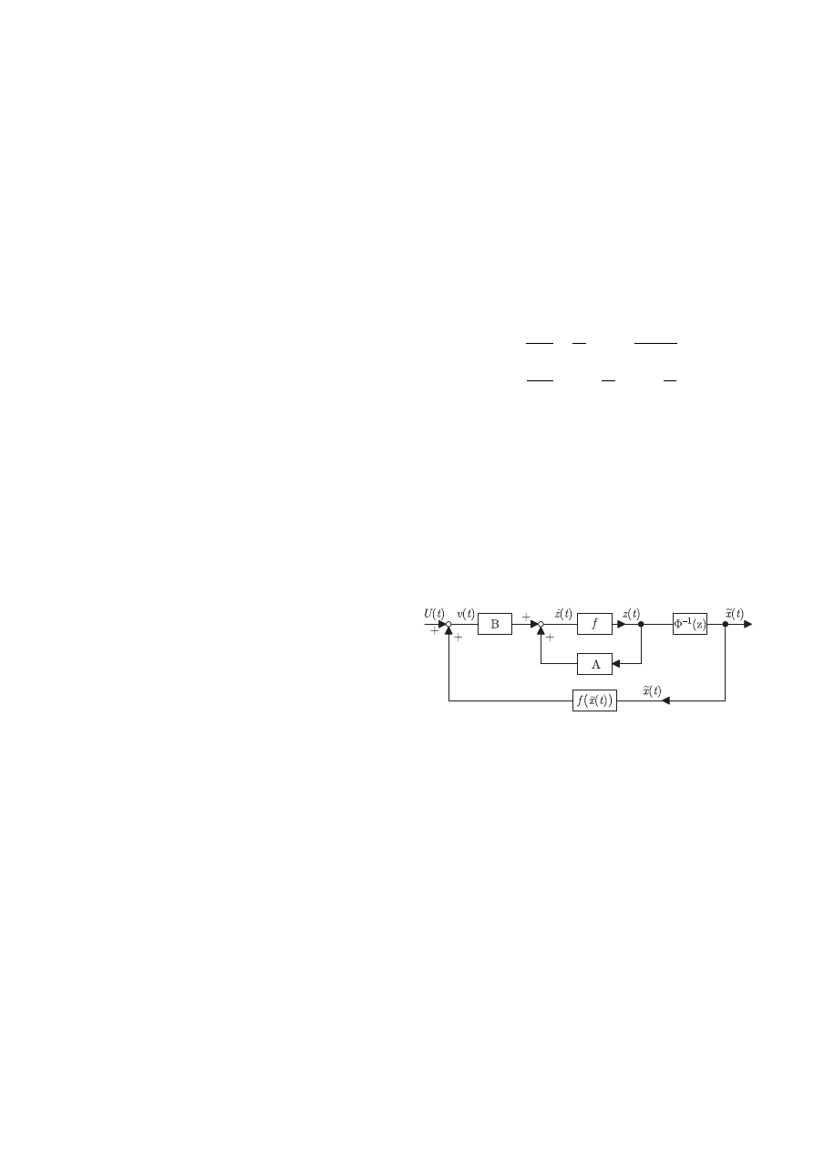
To solve the system (38–40) we use the iterative method

which is explained in the block diagram in Fig. 15.

Fig. 15. Block diagram of linear system with the new input

v = u + f (˜

x)

For the numerical solution the following recurrent model is

applied

v

i+1

= b

i

u

i

+ f (˜

x

i

),

i = 0, 1, 2, ..., N

(41)

z

i+1

= Az

i

+ Bv

i+1

,

i = 0, 1, 2, ..., N

(42)

z

0

= φ(x

0

)

(43)





˜

x

1

˜

x

2

˜

x

3



 =





h

1

z

1,i

+ h

2

z

2,i

+ h

3

z

3,i

h

4

z

1,i

+ h

5

z

5,i

z

1,i





i = 0, 1, ..., N

(44)

The iterative solution of equation

z

i+1

= Az

i

+ Bv

i+1

(45)

is presented in Appendix 1.

Numerical analysis. For the calculations the parameter

values (11) of the circuit shown in Fig. 1 are assumed. The

68

Bull. Pol. Ac.: Tech. 54(1) 2006

Linearization of non-linear state equation

difference between the numerical solution of Eq. (31) and that
of Eqs. (41–44) can be characterized by the norm

kxk

max

= max

16i6N

kx

i

k

(46)

in this case

kx

1

(t) − ˜

x

1

(t)k

max

6 ε

1

kx

2

(t) − ˜

x

2

(t)k

max

6 ε

2

kx

3

(t) − ˜

x

3

(t)k

max

6 ε

3

.

(47)

Comparing the numerical solutions of Eq. (31) with Eqs. (41–
44) we notice that the curves of state variables x

1

(t) = V

p

(t),

x

2

= I

M

(t) and x

3

= Ω(t) are identical. It results from small

error values ε

1

, ε

2

, ε

3

, shown in Table 1, where h is the inte-

gration step in Runge-Kutta method. This method is also used
to solve non-linear Eq. (31) as well as in the numerical imple-
mentation of the algorithm (41–44).

Table 1

The dependence of errors (42) on the value of the integration

step h

h

ε

1

ε

2

ε

3

1.0 e-5

2.62705 e-02

1.5124 e-04

2.323 e-04

1.0 e-6

2.59553 e-03

1.517 e-05

2.336 e-05

1.0 e-7

2.5924 e-04

1.52 e-06

2.34 e-06

1.0 e-8

2.592 e-05

1.6 e-07

2.4 e-07

5.3. Generalization of a global linearization method. Let
the

x =





x

1

x

2

x

3





be the state vector, and u ∈ R be a scalar function. We assume
that the state equation can be presented as follows [5,8,29]:

˙x

1

= φ

1

(x

1

) + x

2

+ g

1

(x, u)

˙x

2

= φ

2

(x

1

, x

2

) + x

3

+ g

2

(x, u)

˙x

3

= φ

3

(x

1

, x

2

, x

3

) + g

3

(x, u); x(0) = x

0

,

(48)

where the functions φ

k

and g

k

∈ C

1

for k = 1, 2, 3. To obtain

the linear equation, we define the following change of variables

z =





z

1

z

2

z

3



 =





x

1

φ

1

(x

1

) + x

2

φ(x

1

, x

2

) + x

3



 = φ(x),

z (0) = φ [x (t = 0)] .

(49)

The inverse transformation that expresses the vector x in

the function of vector z is the following

x =





x

1

x

2

x

3



 =





z

1

z

2

− φ

1

(z

1

)

z

3

− φ

2

(z

1

, z

2

− φ

1

(z

1

)



 = φ

−1

(z). (50)

Using (48) and (49), after necessary transformations, we have:





˙z

1

˙z

2

˙z

3



 =





0

1

0

0

0

1

−k

1

−k

2

−k

3









z

1

z

2

z

3



 +





g

1

(x, u)

¯

g

2

(x, u)

¯

g

3

(x, u)



 ,

(51)

z (0) = φ [x (t = 0)]

(52)

or

˙z = Az + g(x, u)

(53)

where:

g(x, u) =





g

1

(x, u)

¯

g

2

(x, u)

¯

g

3

(x, u)





(54)

¯

g

2

(x, u) =

∂φ

1

∂x

1

[φ

1

(x

1

) + x

2

+ g

1

(x, u)] + g

2

(x, u) (55)

¯

g

3

(x, u) =

∂φ

2

∂x

1

[φ

1

(x

1

) + x

2

+ g

1

(x, u)]

+

∂φ

2

∂x

2

[φ

2

(x

1

, x

2

) + x

3

+ g

2

(x, u)]

+ φ

3

(x

1

, x

2

, x

3

) + g

3

(x, u)

+ k

1

z

1

+ k

2

z

2

+ k

3

z

3

.

(56)

Parameters k

1

, k

2

and k

3

are chosen in such a way as to

ensure the stability of matrix A. These parameters allow us to
analyse the linear circuit dynamics and by the same time the
dynamics of the non-linear system. In practice the choice of
the parameters k

1

, k

2

and k

3

depends on the changes of the

values of parameters of non-linear circuits, which are deter-
mined by the circuit structure and influence of some physical
quantities e.g. temperature.

The numerical example. We consider once more the same

example presented in Fig. 1 and described by Eq. (8). Having
carried out some basic transformations, we obtain the follow-
ing set of equations:





˙z

1

˙z

2

˙z

3



 =





0

1

0

0

0

a

2

−k

1

−k

2

−k

3









z

1

z

2

z

3



 +





g

1

(x, u)

¯

g

2

(x, u)

¯

g

3

(x, u)





z

1

(0) = V

p

, z

2

(0) = −a

1

e

aV

p

, z

3

(0) = a

3

V

p

(57)

or

˙z = Az + g(x, u)

(58)

where

g(x, u) =





g

1

(x, u)

¯

g

2

(x, u)

¯

g

3

(x, u)



 .

(59)

In matrix A of Eq. (57) the parameter a

2

(a

2

= 1/C) is in-

troduced by means of transformation (49) in order to analyse
the influence of capacity C on the dynamics of the non-linear
circuit.

On the other hand, the transformation z = φ(x) can be

built in such a way as to obtain the element of A, a

23

= 1.

However, this transformation lengthens the computation time
due to a more complex form of ¯

g

2

(x, u). In this case, we have

φ

1

(x

1

) = −a

1

e

ax

1

φ

2

(x

1

, x

2

) = a

3

x

1

− a

4

x

2

φ

3

(x

1

, x

2

, x

3

) = a

6

x

2

− a

7

x

3

(60)

Bull. Pol. Ac.: Tech. 54(1) 2006

69

A.J. Jordan

¯

g

1

(x, u) = g

1

(x, u) = u

¯

g

2

(x, u) = aa

1

e

ax

1

(a

1

e

ax

1

+ a

2

x

2

− u)

− (1 + a

2

) · (a

3

x

1

− a

4

x

2

− a

5

x

3

)

¯

g

3

(x, u) = a

6

x

1

− a

1

a

4

e

ax

1

− (a

2

a

4

+ a

5

a

6

)x

2

+ a

5

a

7

x

3

+ a

3

u.

(61)

To analyse the influence of the electric circuit parameters

on the circuit dynamics we assume the following form of k

1

,

k

2

and k

3

for matrix A:

k

1

= a

6

=

K

x

J

,

k

2

= a

4

− a

3

=

1

L

(R

m

− 1),

k

3

= a

4

=

R

m

L

(62)

where J is the inertia moment, L and R

m

denote the induc-

tance and resistance of the rotor respectively, and K

x

is the

coefficient of the DC coil.

The eigenvalues of matrix A are investigated depending on

the hypothetical changes of resistance R

m

(R

m

= 12.045 Ω is

the rated resistance). Assuming R

m.1

= 3 Ω and R

m.2

= 25 Ω

we obtain the following eigenvalues:

R

m.1

: λ

1

= −25.08, λ

2

= −2.46 + j199.68,

λ

3

= −2.46 − j199.68

R

m.2

: λ

1

= −2.09, λ

2

= −123.96 + j681.26,

λ

3

= −123.96 − j681.26.

If we change the capacity C (C = 500 µF is the rated capacity)
the eigenvalues are as follows:

C = 1000 µF : λ

1

= −4.45, λ

2

= −57.95 + j326.44,

λ

3

= −57.95j − 326.44.

For the R

m

= 12.045 Ω and the other rated parameters:

λ

1

= −4.99, λ

2

= −57.73 + j443.84,

λ

3

= −57.73 − j443.84.

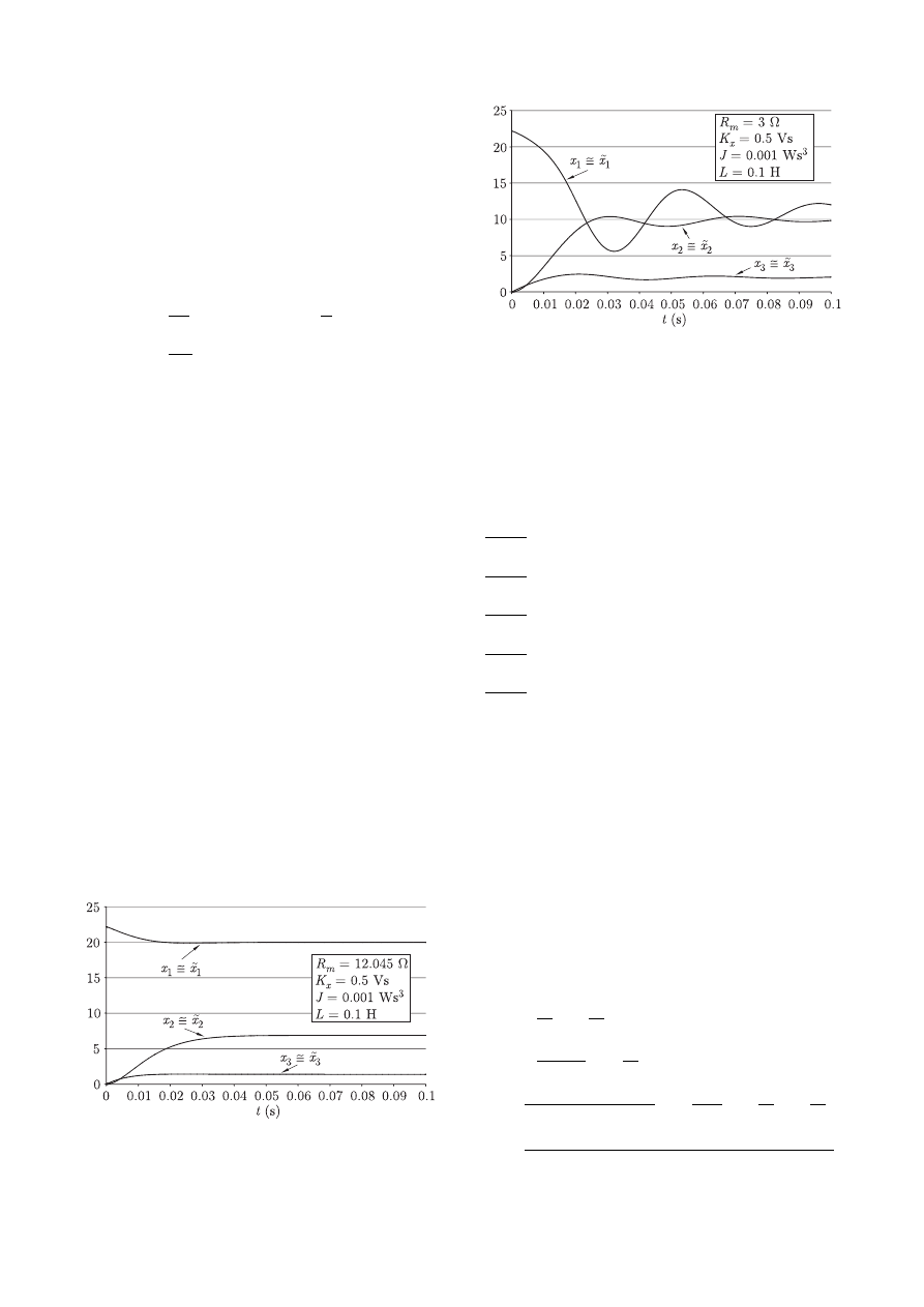
The diagrams showing x

1

(t) ∼

= ˜

x

1

(t), x

2

(t) ∼

= ˜

x

2

(t) and

x

3

(t) ∼

= ˜

x

3

(t) for the rated parameters and for R

m.1

= 3 Ω

are presented in Fig. 16 and in Fig. 17.

Fig. 16. The diagram presenting solution of linear equation with rated

parameters and solution of linear equation with R

m.1

= 3 Ω

Fig. 17. The diagram presenting solution of linear equation with

R

m.1

= 3 Ω

5.4. Another example of the computations.

Below we

would like to show other applications of the global lineariza-
tion method.
Analysis of the dynamic of asynchronous slip-ring motor.
In this case we consider the following set of the non-linear
equations [18]

dx

1

(t)

dt

= −a

1

x

1

− a

5

x

2

+ a

4

x

3

− b

4

x

2

x

5

− b

3

x

4

x

5

+ e

1

dx

2

(t)

dt

= a

5

x

1

− a

1

x

2

+ a

4

x

4

+ b

4

x

1

x

5

+ b

3

x

3

x

5

+ e

2

dx

3

(t)

dt

= a

2

x

1

− a

3

x

3

− a

5

x

4

+ b

2

x

2

x

5

+ b

1

x

4

x

5

− e

3

dx

4

(t)

dt

= a

2

x

2

+ a

5

x

3

− a

3

x

4

− b

2

x

1

x

5

− b

1

x

3

x

5

− e

4

dx

5

(t)

dt

= −c

2

x

5

+ c

1

x

1

x

4

− c

1

x

2

x

3

− M

(63)

where:
x

1

(t), x

2

(t) – the standard form of the stator current,

x

3

(t), x

4

(t) – the standard form of the rotor current,

x

5

(t) – the angular velocity.

Using the global linearization method we obtain the fol-

lowing linear equation:













˙z

1

˙z

2

˙z

3

˙z

4

˙z

5













=













0

1

0

0

0

0

0

1

0

0

0

0

0

1

0

0

0

0

0

1

−k

1

−k

2

−k

3

−k

4

−k

5

























z

1

z

2

z

3

z

4

z

5













+













g

1

(x, u)

¯

g

2

(x, u)

¯

g

3

(x, u)

¯

g

4

(x, u)

¯

g

5

(x, u)













(64)

An inverse transformation:

x

1

= z

1

x

2

= −

a

1

a

5

z

1

−

1

a

5

z

2

x

3

= −

a

2

1

+ a

2

5

a

5

z

1

−

a

1

a

5

z

2

+ z

3

x

4

=

a

2

a

5

+ a

3

¡

a

2

1

+ a

2

5

¢

a

2

5

z

1

+

a

1

a

3

a

2

5

z

2

−

a

3

a

5

z

3

−

1

a

5

z

4

x

5

=

a

1

a

2

a

5

+

¡

a

2

1

+ a

2

5

¢

a

2

5

+ a

2

a

3

a

5

+

¡

a

2

1

+ a

2

5

¢

a

2

3

a

2

5

z

1

70

Bull. Pol. Ac.: Tech. 54(1) 2006

Linearization of non-linear state equation

+

a

2

a

5

+ a

1

a

2

5

+ a

1

a

2

3

a

2

5

z

2

−

a

2

3

+ a

2

5

a

5

z

3

−

a

3

a

5

z

4

+ z

5

.

(65)

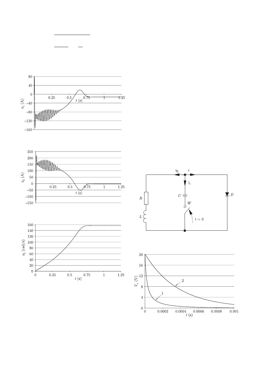
The solutions of non-linear and linear equations are pre-

sented in Figs. 18–20. We should note that the solutions of
both equations are identical.

Fig. 18. The diagram of stator current

Fig. 19. The diagram of rotor current

Fig. 20. The diagram of angular velocity

The electrical circuit with non-linear diode. The anal-

ysed non-linear electrical circuit containing a diode with non-
linear characteristic is presented in Fig. 21 [28].

In the considered case the non-linear characteristic of the

diode is as follows

i = av

c

+ bv

2

c

(66)

Assuming

x

1

= v

c

, and x

2

= i

R

(67)

we have the following set of the non-linear equations

˙x

1

= −a

1

x

1

− a

2

x

2

1

− a

3

x

2

(68)

˙x

2

= a

4

x

1

− a

5

x

2

,

x

1

(0) = V

c,0

, x

2

(0) = 0.

Using the change of state variables defined as follows

z

1

= x

2

z

2

= a

4

x

1

− a

5

x

2

(69)

and after some transformations, we obtain the linear equations

·

˙z

1

˙z

2

¸

=

·

0

1

−k

1

−k

2

¸·

z

1

z

2

¸

+

·

0
v

¸

(70)

where:

k

1

= a

1

a

5

+ a

3

a

4

, k

2

= a

1

+ a

5

v = (−a

1

− 2a

2

x

1

) ˙x

1

− a

3

˙x

2

+ k

1

x

1

+ k

2

(−a

1

x

1

− a

2

x

2

1

− a

3

x

2

).

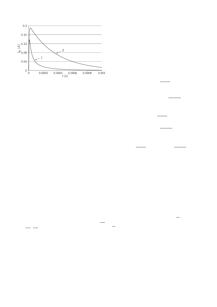
(71)

The diagrams of x

1

(t) = v

c

(t), x

2

(t) = i

R

(t) are shown in

Figs. 22 and 23.

Fig. 21. Electric circuit with non-linear diode

Fig. 22. The diagram of capacitor voltage

Bull. Pol. Ac.: Tech. 54(1) 2006

71

A.J. Jordan

Fig. 23. The diagram of resistor current

In this case curve 1 shows both the non-linear solution and

linear solution. Curve 2 shows the solution of the linear equa-
tion for b = 0.

6. Conclusions

In this paper several methods of the linearization of non-linear
state equation have been presented. Some basic remarks con-
cerning these methods can be made:

– the Taylor’s series expansion assures a good approxima-

tion of non-linear equation for the small ∆x deviations
of the vector x. In the presented example, using Tay-
lor’s series expansion around equilibrium point with the
transient components, a good approximation of the non-
linear equation has been obtained;

– optimal linearization method assures a good approxima-

tion of the non-linear equation, however, it is expensive
(time consuming);

– global linearization method assures convergence of lin-

ear solution with respect to non-linear solution with the
norm maximum [˜

x(t) ∼

= x(t)].

In order to obtain suitable formalism of computations for

the global linearization method, we use the following algo-
rithm resulting from the example presented in section 5.2:

1) introduce non-linear functions f (x, u, t) – the right-

hand side of the non-linear state equation,

2) define and introduce functions: φ

1

, φ

2

, φ

3

and

∂φ

1

∂x

1

,

∂φ

2

∂x

2

,

∂φ

3

∂x

3

,

3) introduce a direct and inverse change of variables:

z = φ(x), ˜

x = φ

−1

(z)

4) define and introduce coefficients k

1

, k

2

, and k

3

.

In the computations we apply the Runge-Kutta method of

the 4

th

order with the integration step h = 10

−6

s for the non-

linear case and h = 10

−11

s for the linear case in the global

linearization method.

The above method can be generalized for the n-

dimensional space (x ∈ R

n

) [8].

Appendix 1

To solve Eq. (35) we can use the following iterative method

z [(k + 1)T ] = e

AT

z(kT )

+ e

A(k+1)T

(k+1)T

Z

kT

e

−Aτ

Bv(τ )dτ

(72)

where

kT 6 t 6 (k + 1)T, k = 0, 1, 2, ...

(73)

Substituting the following relations into Eq. (72)

e

AT

=

∞

X

k=0

(AT )

k

k!

(74)

and

(e

AT

− 1)A

−1

= T

∞

X

k=0

(AT )

k

(k + 1)!

(75)

we obtain

z [(k + 1)T ] =

∞

X

k=0

(AT )

k

k!

z(kT )

+ T

∞

X

k=0

(AT )

k

(k + 1)!

Bv(kT ).

(76)

Using equations

A

1

=

∞

X

k=0

(AT )

k

k!

and A

2

= T

∞

X

k=0

(AT )

k

(k + 1)!

(77)

we calculate the sums of the series (77) according to the con-
vergence criterion:

kS

k+1

k − kS

k

k 6 ε, i.e ε = 10

−5

(78)

kSk = max

j

P

l

a

ij

, where a

ij

are elements of matrix A

1

and

matrix A

2

. Finally, we obtain the following recurrent equation

z(k + 1) = A

1

z(k) + A

2

Bv(k).

(79)

Appendix 2

D

EFINITION

1. A replacement of the non-linear system

(1) by its linear approximation ∆ ˙

x(t) = A∆x(t) + B∆u(t)

is called the “linearization by the Taylor’s series expansion”

of the non-linear system (1), where A =

∂f
∂x

¯

¯

¯

¯

x=x

eq

u=u

eq

, B =

∂f
∂u

¯

¯

¯

¯

x=x

eq

u=u

eq

and the non-linear part R = 0.

D

EFINITION

2. The linear equation obtained by neglecting

the non-linear part R of Eq.(1) is called the linear approxima-
tion of the non-linear system.

D

EFINITION

3. If the norm kx

i,L

(t) − x

L,N L

(t)k

max

is

less than prescribed value ε, i.e. kx

i,L

− x

i,N L

k

max

< ε than

the non-linear system is called weakly non-linear one, other-
wise it is called strongly non-linear:
x

i,L

− i

th

state variable of the linear system,

x

i,N L

− i

th

state variable of the non-linear system.

72

Bull. Pol. Ac.: Tech. 54(1) 2006

Linearization of non-linear state equation

D

EFINITION

4. The system (1) is called BIBS (bounded-

input bounded state ) stable if for any bounded (norm) input u
the state vector x is also (norm) bounded, i.e.

kuk < M implies kxk < N for some finite numbers M > 0

and N > 0 where kk denotes the norm of vector.

(80)

T

HEOREM

3. (T. Kaczorek) [8]. The closed-loop nonlin-

ear system is BIBS stable if the following conditions are satis-
fied.

1) There exists a global diffeomorphism such that (28)

holds for v = u + f (x). This diffeomorphism is defined as
follows:

z = φ(x) =









φ

1

(x)

φ

2

(x)

...

φ

n

(x)









(81)

with the following properties:
i) φ(x) is invertible, i.e. there exists a function φ

−1

(z) such

that

φ

−1

(φ(x)) = x for all x in R

n

(82)

ii) φ(x) and φ

−1

(z) are both smooth mappings (have continues

partial derivatives of any order).

A given transformation (81) is a global diffeomorphism if

it is a smooth function in R

n

and the jacobian matrix

∂φ
∂x

=





∂φ

1

∂x

1

...

∂φ

1

∂x

n

.....................

∂φ

n

∂x

1

...

∂φ

n

∂x

n





(83)

is non-singular for all x in R

n

.

2) The function f (x) is continuous and bounded for all x

in R

n

.

3) All eigenvalues of matrix A have negative real parts.
4) The function x = φ

−1

(z) is bounded for all z in R

n

and

t ∈ [0, +∞].

Acknowledgements. This work was carried out within the
frame of KBN Grant No: 3 T10A 066 27.

R

EFERENCES

[1] R.W. Brockett, “Non-linear control theory and differential ge-

ometry”, Proc. Int. Congress of Mathematicians, Vol. II, 1357–
1368, Polish Scientific Publishers, Warsaw, 1984.

[2] S.P. Banks and M. Tomas-Rodriguez, “Linear approximation to

non-linear dynamical systems with applications to stability and
spectral theory”, IMA Journal of Mathematical Control and In-
formation 20, 89–103 (2003).

[3] A.J. Krener and A. Isidori, “Linearization by output injection

and non-linear observers”, Systems Control Letters 3 (1), 47–52
(1983).

[4] T. Kaczorek, A. Dzieli´nski, L. D ˛

abrowski, and R. Łopatka, The

Basis of Control Theory, WNT, Warsaw, 2004, (in Polish).

[5] A. Jordan and J.P. Nowacki, “Global linearization of non-linear

state equations”, International Journal Applied Electromagnet-
ics and Mechanics 19, 637–642 (2004).

[6] A. Isidori, Non-linear Control Systems, Springer Verlag, 1995.

[7] R. Marino and P. Tomei, Non-linear Control Design – Geomet-

ric, Adaptive, Robust, Prentice Hall, 1995.

[8] T. Kaczorek and A. Jordan, “Global stabilization of a class of

non-linear systems”, in.: Computer Application in Electrical
Engineering, ed. R. Nawrowski, Pozna´n University of Technol-
ogy, (to be published).

[9] C. Navarro Hernandez and S.P. Banks, “Observer designer for

non-linear systems using linear approximations”, IMA Journal
of Mathematical Control and Information 20, 359–370 (2003).

[10] A. Jordan et. al., “Optimal linearization method applied to the

resolution of non-linear state equations”, RAIRO – Automa-
tique, Systems Analysis and Control 21, 175–185 (1987).

[11] A. Jordan et al., “Optimal linearization of non-linear state equa-

tions”, RAIRO – Automatic Aystems Analysis and Control 21
(3), 263–272 (1987).

[12] B. Jakubczyk and W. Respondek, Geometry of Feedback and

Optimal Control, Marcel Dekker, New York,1998.

[13] T. Kaczorek, A. Jordan, and P. Myszkowski, “The approxima-

tion of non-linear systems by the use of linear time varying sys-
tems”, IC-SPETO Conference, (to be published).

[14] W. Kang and A.J. Krener, “Extended quadratic controller nor-

mal form and dynamic state feedback linearization of non-linear
systems”, SIAM J. Control Optim. 30(6), 1319–1337 (1992).

[15] F. Plestan and A. Glumineau, “Linearization by generalized

input-output injection”, Systems Control Letter 31 (2), 115–128
(1997).

[16] P. Kokotovic and M. Arcak, “Constructive non-linear control:

A historical prospective”, Automatica 37, 637–662 (2001).

[17] W. Gear, Numerical Initial Value Problems in Ordinary Differ-

ential Equations, Prentice – Hall. Inc, 1971.

[18] B. Baron, A. Marcol, and S. Pawlikowski, Numerical Methods

in Delphi, Helion, Gliwice, 1999, (in Polish).

[19] Z. Fortuna, B. Macukow, and J. W ˛

asowski, Numerical Methods,

WNT, Warszawa, 2002, (in Polish).

[20] A. Krupowicz, Numerical Methods for Initial Value Problems

in Ordinary Differential Equations, PWN, 1986, (in Polish).

[21] S.H. Zak, Systems and Control, Oxford University Press, 2003.
[22] T. Kaczorek, The Control and Systems Theory, PWN, Warsaw,

1996, (in Polish).

[23] W.J. Cunnigham, Introduction to Non-linear Analysis, WNT,

Warsaw, 1962, (in Polish).

[24] M. Barland et al., “Commende optimal d’un systeme generateur

photovoltaique convertisseur statique – recepteur”, Revue Phys.
Appl. 19, 905–915, Commision des Publications Francaises de
Physique, Paris, 1984.

[25] A. Jordan et al., “Optimal linearization of non-linear state equa-

tions”, RAIRO – Automatic Systems Analysis and Control 21,
263–272 (1987).

[26] B.N. Datta, Numerical Methods for Linear Control Systems

– Design and Analysis, Elsevier Academic Press, New York,
2004.

[27] A. Jordan et. al, “Optimal linearization method applied to the

resolution of non-linear state equations”, RAIRO – Automa-
tique, Systems Analysis and Control 21, 175–185 (1987).

[28] A. Jordan and J.P. Nowacki, “Global linearization of non-linear

state equations”, International Journal Applied Electromagnet-
ics and Mechanics 19, 637–642 (2003).

[29] T. Kaczorek, “The introduction to the Lie algebra”, The Semi-

nary in the Technical University of Bialystok, 2003, (not pub-
lished).

Bull. Pol. Ac.: Tech. 54(1) 2006

73