arXiv:1011.5744v2 [cond-mat.soft] 30 Nov 2010

Non-linear rheology of active particle suspensions: Insights from an analytical

approach

Sebastian Heidenreich

∗

Rudolf Peierls Centre for Theoretical Physics, University of Oxford,

1 Keble Road, Oxford OX1 3NP, United Kingdom and

Institut f¨

ur Theoretische Physik, Sekr. EW7-1, Technische Universit¨

at 10623 Berlin, Hardenbergstrasse 39, Berlin, Germany

Siegfried Hess and Sabine H. L. Klapp

Institut f¨

ur Theoretische Physik, Sekr. EW7-1, Technische Universit¨

at 10623 Berlin, Hardenbergstrasse 39, Berlin, Germany

(Dated: December 1, 2010)

We consider active suspensions in the isotropic phase subjected to a shear flow. Using a set

of extended hydrodynamic equations we derive a variety of analytical expressions for rheological
quantities such as shear viscosity and normal stress differences. In agreement to full-blown numerical
calculations and experiments we find a shear thickening or -thinning behaviour depending on whether
the particles are contractile or extensile. Moreover, our analytical approach predicts that the normal
stress differences can change their sign in contrast to passive suspensions.

INTRODUCTION

Within the last years the physics of active materials has become a focus of growing interest. In an active system,

each particle (constituent) ”constantly absorbs energy from its surroundings or from an internal fuel tank (such as
adenosinetriphosphate) and dissipates it in a process of carrying out translational or rotational motion” [8]. The
resulting, continuous energy flux drives an active system out of equilibrium even in a steady state. This is in sharp
contrast to the physics of ”passive” soft-matter systems where non-equilibrium behavior typically occurs only in the
presence of an external driving force (such as shear).

Active systems often occur in biological contexts, examples being acto-myosin filaments, cytoskeletal gels interacting

with motors, bacterial colonies, and swarming fishes [1–3]. Moreover, there are also non-biological representatives such
as vibrated granular rods [4, 5] or remotely powered, self-propelled particles [6].

The individual motion of an active particle through the suspension gives rise to flow fields which, on long time

scales, can be modeled by force dipoles n [7, 8]. The combination of this directed motion and interactions between
active particles (e.g., excluded volume interactions or hydrodynamic interactions) generates rich collective behaviour
with some similarities to that of ordinary ”passive” liquid crystals. However, active systems (”living liquid crystals”
[9]) have fascinating additional features such as an instability of homogeneous, nematic states [10] or the occurrence
of spontaneous flow states in films above a critical thickness [11–16].

Modeling these phenomena on a microscopic level is still a challenge [3]. As an alternative, the collective behavior is

often studied via a coarse-grained continuum approach familiar from liquid-crystal theory. Within this framework the
relevant dynamic variables are the tensorial orientational order parameter Q

µν

= hn

i [8, 17] (where n

describes

the particle orientation and . . . indicates the symmetric traceless part of a tensor), the velocity field, the stress tensor
σ

µν

, the density (if the latter is allowed to vary), and optionally, the polarization of the system [1, 8, 14, 16, 21, 22].

The latter becomes particularly important in systems of so-called ”movers” such as fishes and bacteria. The resulting
hydrodynamic equations are then supplemented by additional terms which take into account the active nature of
the system (see, e.g., Refs. [8, 12, 17]). As a minimal ansatz it is often assumed that the individual force dipoles
generate a contribution to the stress tensor which is linear in Q

µν

. The prefactor can be either positive or negative

describing, respectively, ”contractile” systems (such as suspensions of alga Chlamydomonas Reinhardii, cytoskeletal
rods, actomyosin) or ”extensile” particles (e.g., E. Coli bacteria).

In the present work we use a hydrodynamic approach to explore the non-linear response of an active material to an

external

shear flow. We focus on a non-polar material composed of ”shakers” (such as melanocytes or symmetric rods)

and neglect any variations in the number density. The passive contributions to the equations of motion are modeled in
the spirit of our earlier work on passive liquid-crystalline systems (see, e.g., [23–25]). Activity is then incorporated by
the above-mentioned stress term plus the lowest-order contribution to the order parameter itself. Previous theoretical

∗

Electronic address: s.heidenreich1@physics.ox.ac.uk

investigations on the rheology of active liquid-crystals have already indicated that their flow behavior is more complex
than that of the corresponding passive system. On top of the above-mentioned spontaneous flow one observes, e.g.,
activity-induced shear band formation [16, 17], hydrodynamic instabilities [9, 10], fluid mixing [26], pattern formation
in steady states [27, 28] and cell-sorting phenomena [29].

Contrary to many of these studies, which often involve quite complex numerical investigations, we aim to derive

analytical

results. The focus is on experimental accessible quantities such as the shear viscosity and the normal

stress differences. Our motivation to approach these quantities from an analytical side is to establish simple ”rules”
for the role of, e.g., the prefactor of the activity-induced pressure term, on the non-Newtonian viscosity. We hope
that the physical insight gained by such simple rules may be particularly interesting for the interpretation of future
experiments. Moreover, the results can also serve as benchmark for more complex numerical studies. Of course,
the derivation of explicit expressions is impossible for the full, nonlinear set of hydrodynamic equations. The main
assumption in our work is that the system is close to the passive isotropic state. From a physical point of view this
means that we are essentially restricted to the investigations of states which are isotropic in passive equilibrium in the
absence of external flow. Despite this assumption, our theory shows a variety of non-linear flow phenomena such as
shear thickening and shear thinning in dependence of the activity parameter. Moreover, the theory yields novel results
for the normal stress differences, which are a characteristic rheological feature of any soft-matter system beyond the
linear-response (Newtonian) regime.

The remainder of this paper is organized as follows. In section II we present our set of hydrodynamic equations and

motivate (following the arguments in earlier studies) the extra terms due to activity. Section III deals with the shear
viscosity (in a slab geometry), focussing on a spatially homogeneous system. Here we present analytical expressions
and discuss our results in the light of earlier, fully numerical studies. Section III B is devoted to the normal stress
differences on the same level of approximation.

II.

MODEL EQUATIONS

In the continuum limit the orientational dynamics of active particle suspension is governed by a coarse-grained

equation of motion for the second-rank order parameter Q

µν

[8]. The starting point are the well-established relaxation

equations for passive liquid crystals [25], which may then be supplemented by terms reflecting the activity. Including
these effects to lowest order [8, 10], the resulting equation for the time derivative of Q

µν

is given by

(∂

+ v

∇

µν

= ǫ

µλκ

κν

+ 2κΓ

µλ

λν

−

√

2τ

−

µν

−τ

−

µν

△Q

µν

+ λQ

µν

(1)

where we use the Einstein summation convention and the notation v

for the velocity. The first three terms on the

right-side of Eq. (1) describe the impact of the flow on the order parameter. Specifically, Γ

µν

= ∇

is the strain

rate, ω

µν

,the vorticity, and τ

and τ

are relaxation time coefficients, respectively. In the subsequent term in Eq. (1),

µν

= δΦ/δQ

µν

is the ”molecular field”, which is described by the derivative of the Landau-de Gennes (LG) free

energy Φ of a homogeneous, liquid-crystalline system,

Φ =

1
2

A(T )Q

µν

−

r 2

µλ

λν

µν

1
4

C(Q

µν

)

(2)

where A(T ) = α(T −T

) (with T being the temperature) changes its sign at the isotropic-nematic spinodal temperature,

. Note that the definition of a free energy of an active system is, strictly speaking, impossible due to its non-

equilibrium character. We thus consider Φ as the system’s free energy in the ”passive phase”. The next (gradient)
term in Eq. (1) is again borrowed from equilibrium physics; it results from the increase of free energy due to distortions
in the one-constant approximation. The prefactor of this ”elastic” contribution corresponds to the squared elasticity
length, ξ

. So far, the terms in Eq. (1) correspond to those for passive systems (see, e.g., [25]). It is the last term in

Eq. (1) which corresponds to an ansatz for the effect of activity on the orientational order, with λ being a coupling
parameter. For λ > 0 (λ < 0) the order parameter Q

µν

increases (decreases) in time; the case λ > 0 is therefore

sometimes referred to as ”self-aligning”. For a microscopic interpretation of the coefficient λ, see [35].

Some further interpretation arises when we consider this term, which is linear in Q

µν

, together with the lin-

ear term resulting from the derivative of the squared term in the LG free energy.

This yields a contribution

−τ

−

A(T ) + λ

µν

= −τ

−

δ ˜

Φ/δQ

µν

, where ˜

Φ is a pseudo free energy defined by

Φ =

1
2

(A(T ) − λτ

) Q

µν

(3)

From this consideration we see that λ influences the onset of nematic ordering upon cooling the system from high
temperature (i.e., large values of A). Specifically, a positive value of λ effectively increases the spinodal temperature
and thus stabilizes nematic ordering with respect to the passive case. On the other hand, λ < 0 stabilizes the
isotropic (i.e., orientationally disordered) state [14]. We also see from Eq. (3) that for λ > τ

−

A(T ) the isotropic state

is unstable (i.e., δ

Φ/(δQ)

< 0). Finally, Eq. (3) shows that the order of magnitude of λ is given by the inverse of

the relaxation time τ

The fluid velocity field obeys the generalized Navier-Stokes equations

ρ(∂

+ v

∇

= 2η

iso

∂

λµ

+ ∂

λµ

(4)

where ρ is the fluid density, and η

iso

is the first Newtonian viscosity of the passive system. Following earlier studies

(see, e.g. [10, 15]) we model the stress tensor σ

λµ

as a sum of a passive part, σ

, and an active part, σ

, i.e.,

µν

= σ

p
µν

+ σ

a
µν

(5)

The passive part is given by the corresponding liquid-crystal expression [23]

p
µν

= −

√

(Φ

µν

− △Q

µν

)

(6)

−

√

2κQ

µλ

λν

√

2κ ξ

µλ

△Q

λν

(7)

which can be derived from the free energy of the system and the principles of irreversible thermodynamics. The
presence of the active term, σ

, results from the fact that the self-propelled particles in an active system induce flow

fields which are dipolar in character [8, 10]. Here we use the simplest ansatz (for higher-order corrections see [31])

a
µν

= −

T ζQ

µν

(8)

The proportionality constant distinguishes between extensile (ζ > 0) and contractile (ζ < 0) active flow behavior
[8, 15, 17] and is characterized by the strength of the elementary force dipoles. From Eqs. (8) and (4) we then see
that an extensile system opposes the external flow (described by Γ

νµ

), whereas a contractile system enhances it.

Finally, our analysis neglects any fluctuations of the concentration of active particles in the suspension. Clearly

there are conditions, where the dynamics of the concentration field can strongly influences the other variables [16]. The
goal of the subsequent analysis is to investigate the influence of the parameters λ and ζ on experimentally accessible
rheological properties of the active system. In doing this we focus on the passive, isotropic state rather than on the
metastable regime at the isotropic-nematic transition which was studied numerically in Ref. [17].

III.

ANALYTICAL RESULTS

The flow geometry is given by two infinitely extended plates in the x-z-plane, which are separated by a distance

2h along the y direction. We apply a planar Couette flow by moving the upper plate by +v

and the lower by −v

yielding a velocity profile v

= (v(y), 0, 0). Under these conditions the strain-rate tensor simplifies for a linear flow

profile to Γ

µν

= ∂

/2δ

µy

νx

= ˙γ/2δ

µy

νx

, where ˙γ = ∂v/∂y is the shear rate.

To rewrite the tensorial equations of motion Eqs. (1) and (6) in a more explicit way, we express the second-rank

tensors Q

µν

and σ

µν

, which have five independent components, in a tensor basis, e.g., Q

µν

4
a=0

µν

[37]. The

basis tensors are defined by

µν

r 3

z
µ

z
ν

, T

µν

r 1

x
µ

x
ν

− e

y
µ

y
ν

), T

µν

√

x
µ

y
ν

µν

√

x
µ

z
ν

, T

µν

√

y
µ

z
ν

(9)

where, e.g., e

is the µ-component of the unit vector in z-direction.

In the subsequent analysis we assume that the passive system is isotropic in the absence of external flow (i.e.

µν

= 0). In this case the order-parameter expansion in the equilibrium free energy can be truncated after the first

(quadratic) term, yielding only the linear contribution (i.e., Φ

µν

≈ AQ

µν

) in the dynamic equation for Q

µν

. We

also assume, as a first approximation, that the system is spatially homogeneous, that is, △Q = 0. The resulting,
homogeneous equation of Eq.(1 ) for the alignment tensor Q

µν

decouples into equations for the symmetry-adapted

(a= 0, 1, 2) and symmetry-breaking (a= 3, 4) components. The symmetry-breaking components give no contributions
to our rheological quantities. Therefore, we focus on the symmetry-adapted components, that is,

µν

= Q

µν

+ Q

µν

+ Q

µν

(10)

A similarly decoupling occurs for the stress tensor, yielding

µν

= σ

µν

+ σ

µν

+ σ

µν

(11)

Inserting Eq. (10) into Eq. (1) we obtain the following set of equations describing the orientational dynamics in a
homogeneous, isotropic active system:

ΓQ

√

κΓQ

+ Q

= −

Γ + λ

= Γ Q

+ λ

= −

√

κΓ Q

+ λ

(12)

where Γ = τ

˙γ/A. Equations (12) can be solved for the three symmetry-adapted components yielding, e.g.,

(Γ) = −

1 − λ

∗

+ (1 −

1
3

)Γ

(1 − λ

∗

)

−

(13)

Similar expressions result for Q

and Q

. In Eq. (13) we have introduced the dimensionless active parameter λ

∗

λτ

/A related to the aligning term in Eq. (1). Interestingly, there is no dependence of Q

on the other parameter

related to activity, ζ

∗

= ζ/A, which appears in the pressure equation. We note that this is not a consequence of the

linearization, but rather of our assumption of spatial homogeneity (no backflow).

For liquid crystal polymers the shape parameter κ depends on the coupling strength between orientation and fluids

strain rate. In the kinetic approach κ can be related to the relaxation times τ

and τ

[36], i.e. κ = −

√

15τ

/(7τ

Note, in the description of passive liquid crystal polymers the entropy production has to be positive and Onsager’s
symmetry relations apply. As a result τ

, τ

> 0, but τ

can have either sign depending on the particles shape. For

rod-like particle suspensions the relaxation time τ

is negative and for disk-like particles is positive, respectively. For

active suspensions Onsager’s symmetry relations may be broken such that τ

< 0 is possible. However, for simplicity

we only discuss τ

> 0.

Some other features of Eq. (13) can be seen immediately. In the limit Γ → 0 (no external shear flow) Q

vanishes

(as do the other components), consistent with our assumption of a passive isotropic equilibrium system. A special
situation occurs for λ

∗

→ 1, which corresponds to approaching the stability limit of the isotropic phase [see Eq. (3)].

At the same time, the order parameter as determined from Eq. (1) increases to infinity. This behavior contradicts
the physical picture according to which the order parameter is restricted to a finite (saturation) value related to
perfect alignment. Therefore, the limit λ

∗

→ 1 corresponds to a situation where the truncation of the LG free

energy after the quadratic term cannot justified any more, i.e., higher order terms need to be included to guarantee
the existence of a minimum. Later, we will see that this divergence gives rise to a divergence of the viscosity for
both extensile and contractile suspensions. A divergence for contractile suspensions was predicted by Marchetti and
Liverpool [3, 32, 33, 35] and confirmed in numerical simulations by Cates et al. [17].

For extensile suspensions the viscosity drops to zero [17]. As we will later see, a different behavior is predicted

by our model where the viscosity diverges to minus infinity. This unphysical result effectively restricts our study to
values of λ < 1.

TABLE I: Parameters

-0.1 0.1 0.2 0.37

Apparent shear viscosity

The rheological properties of non-Newtonian fluids can be captured experimentally by measuring the shear viscosity

and the normal stress differences. In the geometry used here, the shear viscosity is determined by the xy− component

- 0.6

- 0.4

- 0.2

0.0

0.2

0.4

0.6

- 0.4

- 0.2

0.0

0.2

0.4

New

=0.65

=0.0

=1.0

- 0.6

- 0.4

- 0.2

0.0

0.2

0.4

0.6

- 0.5

0.0

0.5

1.0

New

=-0.5

=0.0

=-1.0

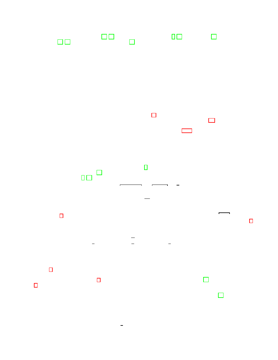
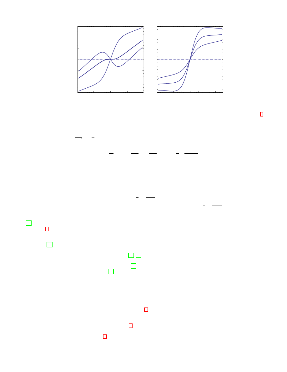
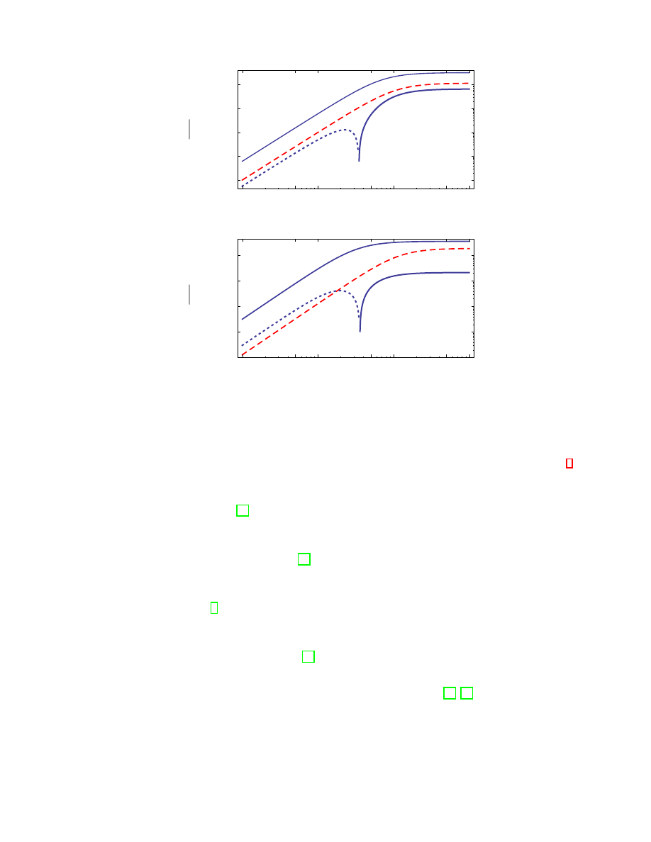
FIG. 1: (Color online) The shear stress vs. shear rate Γ for λ

∗

= 0.7. The remaining parameters are given in table I.

Left: Extensile suspensions show a plateau and negative stress close to zero shear rate. Right: Contractile suspensions are
characterized by a yield stress.

of the stress tensor, i.e. σ

√

2σ

. In terms of the shear rate Γ the shear stress reads

= η

iso

˙γ −

T A

(1 +

∗

−

2
3

1 − λ

∗

2
2

(14)

where η

iso

= (ρ/m)k

T τ

1 − τ

/ (τ

)

is the Newtonian viscosity in a system with Q = 0 (i.e., in an isotropic

state or for systems of spherical particles).

The apparent shear viscosity η is determined by the ratio of shear stress versus the shear rate. For our analysis we

scale η with the (passive) first Newtonian viscosity η

New

= ρ/mk

T τ

, yielding

∗

New

= 1 +






1 − λ

∗

+ (1 +

1
3

)

1−λ

∗

1 − λ

∗

+ (1 −

1
3

)

1−λ

∗

1 − λ

∗

+ (1 −

1
3

)

1−λ

∗

− 1






(15)

For vanishing activity parameters λ

∗

= 0 and ζ

∗

= 0 the apparent shear viscosity of a passive liquid crystal is recovered

[23].

In Fig. 1, the flow curve of our model is shown for extensile and contractile suspensions. For extensile suspensions

there exists a threshold ζ

∗

= 0.55 above which the shear stress shows a plateau. A plateau in the constitutive curve

is frequently used to explain shear banding flow instabilities in passive complex fluids that have been studied for a
long time [19]. The difference here is that the plateau occurs around the zero shear point and the related instability
might generate shear bands with velocities directed in the opposite direction. At the same time the viscosity vanishes
reminiscent to a superfluidic state as discussed in [17, 18].

In a second possible scenario, at a critical nonzero stress −σ

(σ

) the shear rate jumps from a positive (negative)

to a negative (positive) value forming a hysteresis [18]. Hysteresis effects around a positive shear rate value can be
observed for anisotropic complex fluids [20]. In contrast to the passive system for active suspensions the hysteresis
enclose

the zero shear rate point. This means that in a shear stress controlled experiment starting with σ > σ

there is

a threshold before the direction of the velocity can be flipped. A similar effect is not observed in passive suspensions.
The threshold is related to the extra active stress due the active particles orientation and interaction to the solvent.
Contractile suspensions do not show a plateau, but a yield stress which becomes more and more pronounced for higher
values of ζ

∗

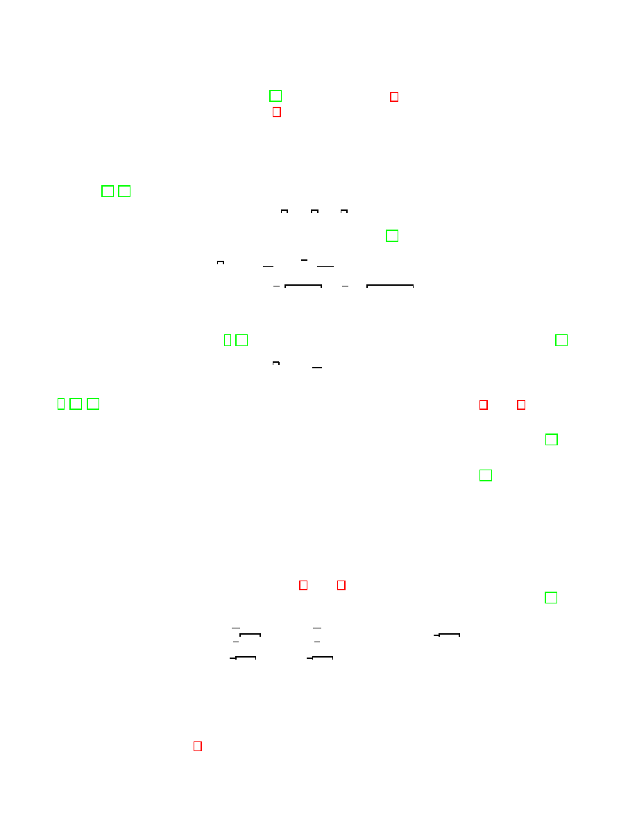
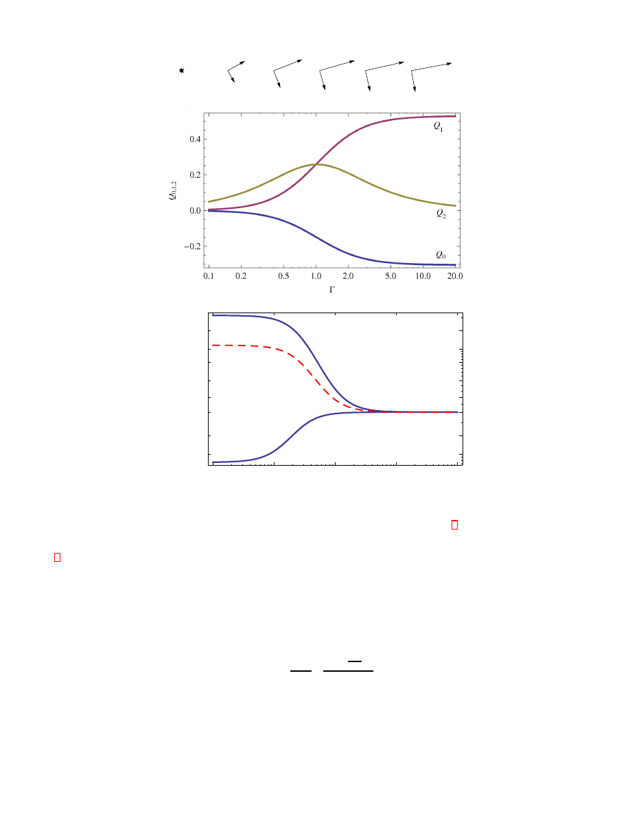
Passive liquid-crystalline systems typically display shear thinning, that is, the shear viscosity decreases with in-

creasing Γ. This is indicated by the red dashed line in Fig. 2. The shear thinning results from the coupling of the flow
gradient and the orientational degrees of freedom, yielding flow-alignment of the suspension. In our model all three
components of the tensorial order parameter are effected. The eigenvectors and eigenvalues indicates the biaxiality
of the flow aligned state. The arrows above Fig. 2 display the eigenvectors multiplied by its eigenvalues. A small
angle is enclosed between the principal director (the eigenvector corresponding to the highest eigenvalue) and the
flow direction. The lower part of Fig. 2 shows the viscosity for extensile and contractile suspensions. Obviously, the

0.01

0.1

100

1.00

0.50

0.20

2.00

0.30

3.00

1.50

0.70

=-0.6

=0.0

= 0.6

FIG. 2: (Color online) Top: The components of the order parameter Q

for parameters given in I. The arrows above the figure

show the eigenvectors of Q. The length is given by the magnitude of the eigenvalues.
Bottom: The scaled viscosity η

∗

vs. shear rate Γ for ζ

∗

= −0.6, 0.0, 0.6 and λ

∗

= 0.7. The remaining parameters given in table

I. The red dashed line indicates shear thinning for the passive suspension.

behavior if η depends very strongly on ζ at low shear rates, but becomes essentially independent at high shear rates.
The intermediate regime is characterized by shear thinning or -thickening behaviour depending on the actual value of
ζ.

For passive liquid crystal polymers in the zero shear limit the viscosity is equal to the the Newtonian viscosity η

iso

However, for active suspensions the zero shear viscosity also depends on active parameters, that is

∗

= 1 −

∗

− 1

(16)

It is remarkable that in the active case the shear viscosity at Γ = 0 strongly differs from the Newtonian case, indicating
the non-equilibrium character of active suspensions.

For contractile suspensions the shear thinning is enhanced and diminished for extensile. For extensile suspensions

there is transition to shear thickening when the zero shear viscosity becomes smaller than the second Newtonian

viscosity η

∗

∞

= 1 − τ

/(τ

). For very high extensile strength the zero shear viscosity can vanish related to the

plateau of the shear stress rate curve Fig. 1. The effect of reduced viscosity was also discussed for a two-dimensional
model of dilute bacterial suspensions in [38]. As mentioned before the high shear rate viscosity reaches the second
Newtonian viscosity independent on the activity.

In our model the shape parameter κ influences the results only marginally. In the special case κ = 0 the shear

viscosity simplifies to

∗

= η

∗

∞

∗

− η

∗

∞

1 + (τ

˙γ)

(17)

where τ

is a characteristic time defined as τ

−

= A/τ

−λ

∗

= 6D

−λ

∗

. Therefore, the activity parameter λ

∗

modifies

the self-rotational diffusion constant D

. The apparent viscosity Eq. ( 17) can be related to a simple rheological shear

thinning model, that is, the Cross model [46]:

η = η

∞

− η

∞

1 + (C ˙γ)

(18)

For our model we find C = τ

and m = 2.

The simplified formula (17) gives us the possibility to link experimentally accessible quantities to our theoretical

parameters λ

∗

and ζ

∗

. Specifically, we need from experiments the zero-shear viscosity, the high-shear viscosity η

∞

, the

rotational diffusion constant, and the relaxation time τ

. The latter can be determined from a fit of the experimental

shear viscosity to Eq. (16). The rotational diffusion constant D

has to be measured in an independent experiment, see

e.g. [44] for rod-like fd-viruses. From these quantities, the activity parameter λ follows via the relation λ

∗

= 6D

−τ

−

Next, the active force acting on the fluid modelled by ζ

∗

is related to λ

∗

via

∗

= (η

∗

− 1)λ

∗

− η

∗

(19)

where we defined the viscosity η

∗

1−η

∗

1−η

∗

∞

. Here the ratio of the relaxation times can be related to the active particles

shape [45], i.e.

= −

3
2

R. The coefficient R measures the non-sphericity of particles. For isolated ellipsoids with

the semi-axes a = b, c and the aspect ratio q = c/b, one has R = (q

− 1)/(q

+ 1).

There is a remarkable symmetry between the particles shape and response to the flow. The rheological properties

do not distinguish between extensile disk-like particles (contractile, rod-like particle) and contractile rod-like particles
(extensile, rod-like particle), respectively.

Normal stress differences

The appearance of normal stress differences indicate strong non-Newtonian behaviour and is related to surprising

rheological effects, e.g., the Weissenberg effect or swelling jets [46]. In our theoretical description we can compute the
normal stress differences from the components of the stress tensor via N

= σ

− σ

and N

= σ

− σ

. In our

notation

= 2σ

= −

√

3σ

− σ

(20)

The analytical expression of the stress tensor components are given by

= −

T A

(1 +

∗

)

ΓQ

1 − λ

∗

−

2
3

(1 − λ

∗

)

2
2

(21)

= −

T A

−

√

(1 +

∗

)

1 − λ

∗

√

2
2

+ (1 −

1
3

)

(1 − λ

∗

)

2
2

(22)

From these relations it follows that

New

= 2






1 − λ

∗

+ (1 +

1
3

)

1−λ

∗

1 − λ

∗

+ (1 −

1
3

)

1−λ

∗

1 − λ

∗

+ (1 −

1
3

)

1−λ

∗






1 − λ

∗

(23)

Similarly N

is given by

New

2κ +

∗

κ −

∗

1 − λ

∗

1 − λ

∗

+ (1 −

1
3

)

1−λ

∗

(24)

−

1 − λ

∗

+ (1 +

1
3

)

1−λ

∗

1 − λ

∗

+ (1 −

1
3

)

1−λ

∗

1 − λ

∗






In passive, nematic liquid-crystal polymers subject to a shear flow the first normal stress difference displays a different
sign depending on the shear rate. The resulting change of sign was first observed in experiments by Porter and Kiss
[39] (see also [40, 42, 43] for further experiments and numerical simulations).

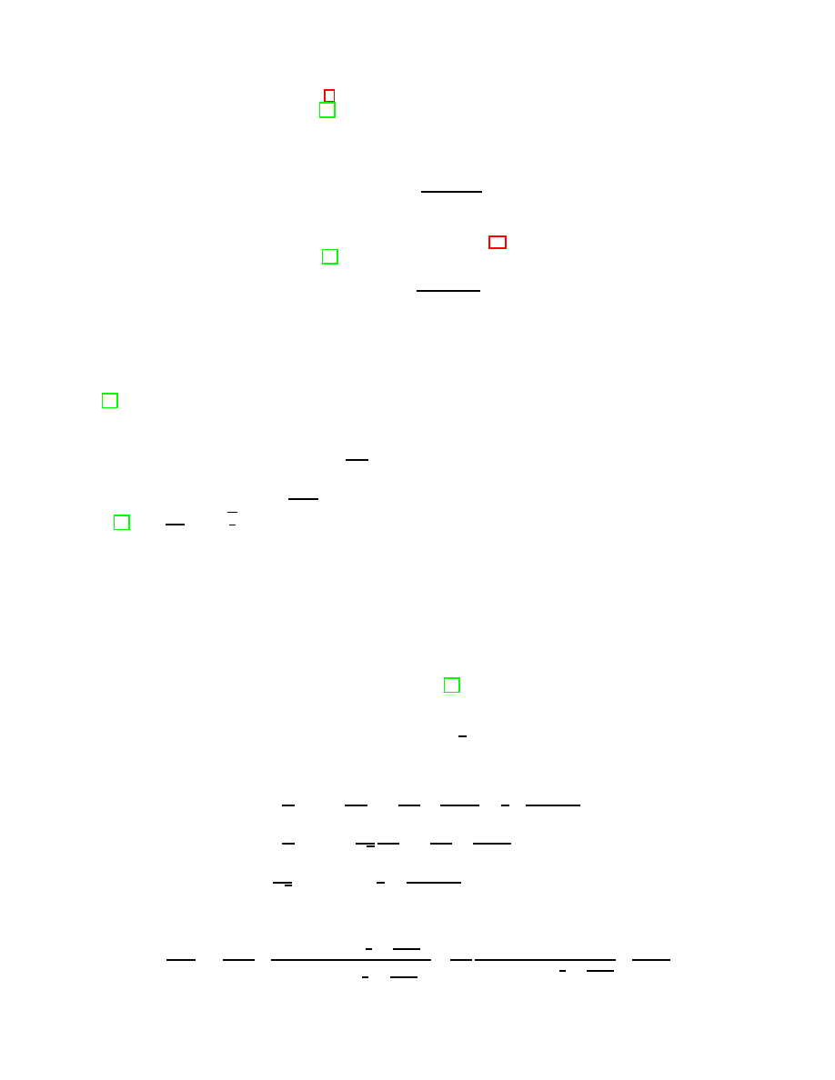
On the other hand, isotropic liquid crystal polymers do not show that sign change. The first (second) normal stress

difference for isotropic liquid crystal polymers is positive (negative) and increases (decreases) with increasing shear
rate. In contrast, active suspensions deep in the isotropic phase can change the sign of the normal stress differences.
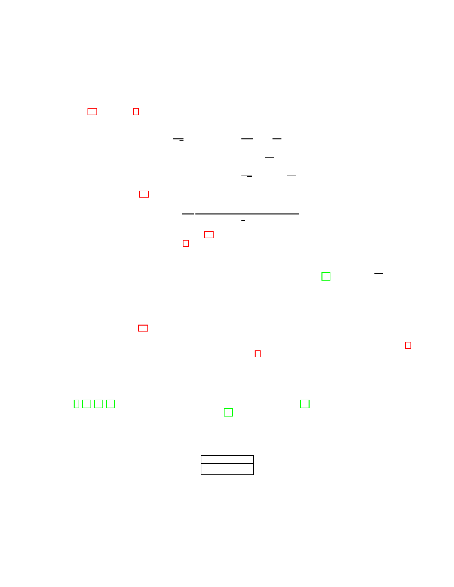
In Fig. 3 the dashed red line shows the dependence of N

and N

on the shear rate for passive liquid-crystal polymers

(i.e., λ = ζ = 0).

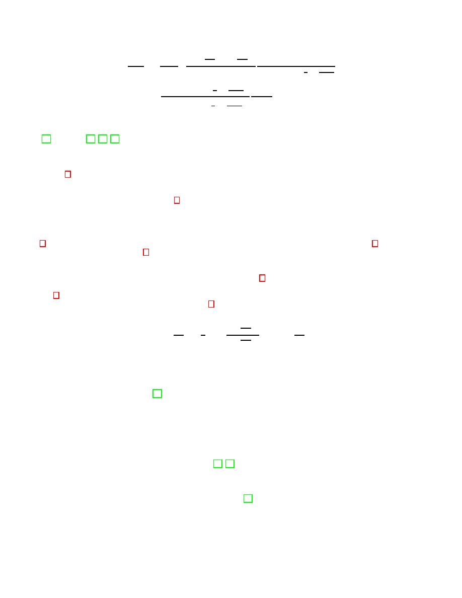
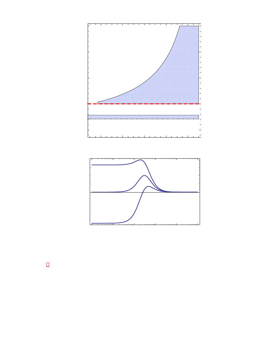
For contractile suspensions there is a parameter range where the sign of the first normal stress difference changes at

low shear rates. The upper panel of Fig 4 shows the relevant parameter range in the λ

∗

− ζ

∗

-plane. The red dashed

line divides the plane in two regions, one of shear thinning and one of shear thickening. The sign change of N

appears

in the shear thinning regime only. The relevant region growth with increasing λ

∗

consistent with the limiting case of

passive nematic liquid crystal polymers (λ

∗

− > 1).

The second normals stress difference for passive suspensions is negative for all shear rates (red dashed line, Fig.

3). However, for active suspension there is a small parameter regime in the shear thickening region (4) that shows a
change in sign as shown in Fig 3. Outside the relevant parameter regions the normal stress difference have the same
qualitative behaviour as their passive counterparts. The difference is a shift that depends on both parameters λ

∗

and

∗

The transition line from shear thickening to shear thinning in Fig. 4 is not sharp. For a fixed λ

∗

value and increasing

parameter, from ζ

∗

= −0.6, a smooth crossover from thickening to thinning in the vicinity of the dashed red line in

Fig 4 (upper panel) can be observed. The smooth crossover is characterized by a small overshoot that growth and
disappears as illustrated in the lower panel of Fig. 4.

In the limit of zero shear, both normal stress differences are vanishing. However, the ratio N

, given by

lim

Γ→0

= −

1
2

1 −

2 +

∗

1 +

∗

= lim

Γ→0

(25)

is a constant. The so-called viscometric functions are related to the normal stress differences by

= N

, Ψ

= N

(26)

The ratio of the viscometric coefficients for κ ≈ 0.4 in the passive limit is estimated to Ψ

/Ψ

≈ −0.1 which is a

value typical for polymeric fluids [47]. The corresponding value for active fluids can vary significantly. For example,
at ζ

∗

= 0.3 one obtains Ψ

/Ψ

≈ 0.2 and for ζ

∗

= −0.3, Ψ

/Ψ

≈ −0.175. This is an additional example for the

different rheological behaviour of active matter.

IV.

CONCLUSION

The analytical approach of our simplified model is able to describe some significant rheological features found earlier

in numerical investigations of more involved models [14, 17]. One important feature concerns the effect of activity on
the zero-shear viscosity which can be significantly larger (contractile) or smaller (extensile) as compared to the passive
case. Therefore, and since the high-shear viscosity is essentially independent of activity, the intermediate shear-rate
regime of active suspensions is characterized by either strong shear thinning (contractile) or thickening (extensile).
Recently, strong shear thinning was experimentally observed [49] in suspensions of Chlamydomonas Reinhardii.

Furthermore, we investigated the normal stress differences and found a remarkable sign change absent in the passive

case. This novel effect is characterized by the activity of the suspension. We predict the sign change for the first
normal stress difference for a wide parameter rage. For example Chlamydomonas Reinhardii may show the predicted
effect due to strong shear thinning and flow aligning effect similar to rod-like passive suspensions. Moreover, we have
shown that the corresponding ratio of the viscometric functions deviates markedly from the passive case.

0.01

0.05 0.10

0.50 1.00

5.00 10.00

-5

-4

0.001

0.01

0.1

New

-N

=0.6

=-0.6

0.01

0.05 0.10

0.50 1.00

5.00 10.00

-5

-4

0.001

0.01

New

=-0.25

=0.25

FIG. 3: (Color online) Top: The first normal stress difference changes its sign for extensile (ζ

∗

= 0.6) active particle suspensions.

The dotted line illuminates negative values of N

. The curve for contractile suspensions is shifted with respect to the curve of

passive suspensions (red dashed line). Bottom: The sign change of the second normal stress difference appears for contractile
suspensions. The dotted line illuminated the positive values of N

. For extensile suspensions there is no sign change, but a

shift with respect to the passive curve (red dashed line). The remaining parameters of both figures are shown in table I.

In the present study we have not considered the impact of spatially inhomogeneity on the rheology of active matter,

although this may clearly be relevant [11]. Here we have rather assumed that inhomogeneities are small and do not
change our predictions qualitatively. Indeed, we have performed some preliminary test of our predictions, using an
one-dimensional, small sine-shaped inhomogeneity. The resulting equations are rather involved and thus not given
here. An explicit numerical investigation is more reasonable and will be presented elsewhere. Note, that in principle
the active parameters may also spatially dependent [48] and probably not independent of each other. However, to our
knowledge there is no rigorous derivation of the parameters from the micro-swimmers that includes the swimming
mechanism.

In our study we assumed that the effective interaction between active particles lead to isotropic and nematic order

as, for example, migrating cells [9]. Similar to the hydrodynamic theory of nematic liquid crystals we coupled the
generalized Navier-Stokes equations to the second rank symmetric traceless order parameter Q. However, in dilute
suspensions when self-driven particles show swarming motion, the symmetry of the particles orientational distribution
leads to a vectorial order parameter P rather than a Q tensor. The rheology for active suspensions related to a
polarization vector P are studied by Giomi et. al. [16]. Similar to our findings the model predicts shear thinning,
thickening and vanishing viscosity. The effect on normal stress differences is not investigated, but we expect no
significantly different results. In a further extension of the theoretical description a coupled vector-tensor model used
for passive polarized nano-rod suspensions may show additional rheological effects [51, 52].

Very recently, Saintillan used a Fokker-Planck approach to model the orientational dynamics of micro-swimmers in

extensional

flows. He models active stress contributions by force dipoles that are generated by swimming strokes of

the individual swimmers. Depending on the extensional rate the suspension shows thinning, thickening and a negative
effective viscosity similar to our results. It is remarkable that, despite different equations used in the passive part of
the pressure tensor and of the orientational dynamics, all models lead to qualitatively the same rheological behavior.

0.0

0.2

0.4

0.6

0.8

0.0

0.5

1.0

1.5

2.0

shear thinning

shear thickening

N2: +-

N1: +-

0.001

0.01

0.1

100

0.5

0.52

0.54

0.56

0.58

=0.48

=0.5

=0.52

FIG. 4: (Color online)Top: Rheological diagram of active suspensions in the plane spanned by the two activity parameters.
The red dashed indicated the activity parameter ζ

that divides the plane in a shear thinning and a shear thickening region.

For shear thickening there is a region that shows sign change of the first normal stress difference. On the other hand, in the
shear thinning regime there exist a parameter range for sign change of the second normal stress difference. The parameter set:
A

= 0.2 and I.

Bottom: The apparent shear viscosity close to ζ

shows a shear thickening and thinning behaviour. The parameter value of

= 0.7.

We expect that the active stress coupling modeled by force dipoles are responsible for the effects discussed here. In
that sense shear thinning, thickening, zero effective viscosity and sign change in the stress differences are general
effects in active soft matter.

We finish with a remark on the relaxation times. The relaxation times of the passive suspension are restricted due

to Onsager’s symmetry relations, viz τ

> 0, τ

> 0 and τ

> τ

. On the other hand active particle suspensions

always dissipate energy due to the process of metabolism. Therefore, a general description needs additional variables
that are related to the process of metabolism and motility of the swimmers. As a consequence, the relations for the

relaxation times in the passive case may be violated.

Acknowledgments

We thank R. Vogel for useful discussions. Financial support within the Collaborative Research Center ”Mesoscopically
structured Composites” (Sfb 448, project B6) and the project HE5995/1-1 of the Deutsche Forschungsgemeinschaft
is gratefully acknowledged.

[1] S. Ramaswamy and R. A. Simha, Sol. State. Comm., 2006, 139, 617-622.
[2] K. Kruse, J. F. Joanny, F. J¨

ulicher, J. Prost, and K. Sekimoto, Phys. Rev. Lett.,2004, 92, 078101/1-4.

[3] T. B. Liverpool and M. C. Marchetti, Phys. Rev. Lett., 2006, 97, 268101/1-4.
[4] V. Narayan, S. Ramaswamy, N. Menon, Science ,2007, 6, 105.
[5] A. Kudrolli, G. Lumay, D. Volfson, and L. S. Tsimring, Phys. Rev. Lett., 2008, 100, 058001/1-4.
[6] S. T. Chang, V. N. Paunov, D. N. Petsev and O. D. Velev, Nature Materials,2007, 6, 235-240.
[7] C. Brennen and H. Winet, Ann. Rev. of Fluid Mech., 1977, 9, 339-98.
[8] Y. Hatwalne, S. Ramaswamy, M. Rao, and R. A. Simha, Phys. Rev. Lett.,2004, 92, 118101/1-4.
[9] H. Gruler, M. Schienbein, K. Franke, and A. DeBoisfleury-Chevance, Mol. Cryst. Liq. Cryst.,1995, 260, 565-574.

[10] R. A. Simha and S. Ramaswamy, Phys. Rev. Lett.,2002, 89, 058101/1-4.
[11] R. Voituriez, J. F. Joanny, and J. Porst, Eur. Phys. Lett.,2005, 70, 404-410.
[12] R. Voituriez, J. F. Joanny, and J. Porst, Phys. Rev. Lett,2006, 96, 028102/1-4.
[13] S. Ramaswamy and M. Rao, New J. Phys.,2007, 9, 423/1-9.
[14] D. Marenduzzo, E. Orlandini, and J. M. Yeomans, Phys. Rev. Lett.,2007, 98, 118102/1-4.
[15] S. A. Edwards and J. M. Yeomans, Eur. Phys. Lett.,2009, 85, 18008/1-6.
[16] L. Giomi, M. C. Marchetti, and T. B. Liverpool, Phys. Rev. Lett.,2008, 101, 198101/1-4.
[17] M. E. Cates, S. M. Fielding, D. Marenduzzo, E. Orlandini, and J. M. Yeomans, Phys. Rev. Lett.,2008,101, 068102/1-4.
[18] L. Giomi, T. B. Liverpool and M. C. Marchetti, Phys. Rev. E, 2010, 81, 051908/1-9.
[19] S. M. Fielding and P. D: Olmsted Phys. Rev. Lett., 2003, 90, 224501/1-4.
[20] S. H. L. Klapp and S. Hess Phys. Rev. E, 2010, 81,051711/1-9.
[21] A. Baskaran and M. C. Marchetti, Phys. Rev. E, 2008, 77, 011920/1-9.
[22] A. Baskaran and M. C. Marchetti, Phys. Rev. Lett.,2008, 101, 268101/1-4.
[23] C. P. Borgmeyer, S. Hess, J. Non-Equlib. Thermodyn.,1995, 20, 259-384.
[24] S. Heidenreich, PhD-thesis, Technische Universit¨

at Berlin 2008.

[25] S. Heidenreich, S. Hess and S. H. L. Klapp, Phys. Rev. Lett.,2009, 102, 028301/1-4.
[26] D. Saintillan and M. J. Shelley, Phys. Rev. Lett.,2008, 100, 178103/1-4.
[27] I. S. Aranson and L. S. Tsimring, Phys. Rev. E,2005, 71, 050901(R)/1-4.
[28] R. Peter, Y. Schaller, F. Ziebert, and W. Zimmermann, New. J. Phys.,2008, 10, 034002/1-16.
[29] J. M. Belmonte, G. L. Thomas, L.G. Brunnet, R. M. C. De Almeida and H. Chate, Phys. Rev. Lett.,2008, 100, 248702/1-4.
[30] Hess and G.D. Bachand, Nanotoday,2005, 8, 22-29.
[31] A. Ahmadi, T. B. Liverpool and M. C. Marchetti, Phys. Rev. E, 2005, 72(R), 060901/1-4.
[32] T. B. Liverpool and M. C. Marchetti, Phys. Rev. Lett., 2003, 90, 138102/1-4.
[33] T. B. Liverpool and M. C. Marchetti, Eur. Phys. Lett., 2005, 69, 846-852.
[34] T. B. Liverpool and M. C. Marchetti, Phys. Rev. Lett., 2006, 97, 268101/1-4.
[35] T. B. Liverpool and M. C. Marchetti, Phys. Rev. E, 2006, 74, 061913/1-23.
[36] S. Hess, Physica A, 1983, 118, 79-104.
[37] P. Kaiser, W. Wiese and S. Hess, J. Non-Equilib. Thermodyn., 1992, 17,153-169.
[38] B. M. Heines, I. S. Aranson, L. Berlyand and D. A. Karpeev, Phys. Biology, 2008, 5,046003/1-9.
[39] G. Porter and R. S. Kiss, J. Polym. Sci.: Polym. Symp.,1978, 65, 193-211.
[40] S. Baek, J. J. Magda, and S. Cementwala, J. Rheol.,1993, 37, 935-945.
[41] J. Ding and Y. Yang, Rheol. Acta, 1994, 33, 405-418.
[42] Y.-G. Tao, W. K. den Otter, J. K. G. Dhont and W.J. Briels, J. Chem. Phys., 2006, 124, 134906.
[43] P. Moldenaers and J. Mewis, J. Rheol., 1986, 30, 567-584.
[44] P. M. Lettinga, Z. Dogic, H. Wang and J. Vermant, Langmuir, 2005, 21, 8048-8057.
[45] A. Peterlin and H. A. Stuard, Hand- und Jahresbuch der Chemischen Physik, volume 8,p.113, Eds. Eucken-Wolf, 1943.
[46] H. A. Barnes, J. F. Hutton and K. Walters, An Introduction to Rheology, Elsevier, London 1989.
[47] R. B. Bird, R. C. Armstrong, O. Hassager amd C. F. Curtiss, Dynamics of polymeric liquids, vol 1/2, J. Wiley, New York

1977.

[48] D. Marenduzzo and E. Orlandini, Soft Matter, 2010, 6, 774-778.
[49] S. Rafai, L. Jibuti and P. Peyla, Phys. Rev. Lett., 2010, 104, 098102/1-4.
[50] D. Saintillan, Phys. Rev. E, 2010, 81, 056307/1-10.
[51] S. Grandner, S. Heidenreich, S. Hess and S. H. L. Klapp, EPJE, 2007, 24, 353-365.
[52] S. Grandner, S. Heidenreich, P. Ilg, S. H. L. Klapp and S. Hess Phys. Rev. E, 2010, 75(R), 040701/1-4.

Document Outline

I Introduction
II Model Equations
III Analytical Results
- A Apparent shear viscosity
- B Normal stress differences
IV Conclusion
References

Wyszukiwarka

Podobne podstrony:
A Comparison of Linear Vs Non Linear Models of Aversive Self Awareness, Dissociation, and Non Suicid
Linearization of non linear state equation
Ladder of citizen participation (en)
Effect of Active Muscle Forces Nieznany
A Novel Switch mode DC to AC Inverter With Non linear Robust Control
Chang S Y A Non linear elliptic equations in conformal geometry (EMS, 2004)(ISBN 303719006X)(O)(100s
Linear and non Linear SR 2012
Far Infrared Energy Distributions of Active Galaxies in the Local Universe and Beyond From ISO to H
Formation of active inclusion bodies in E coli
Ebsco Bialosky Manipulation of pain catastrophizing An experimental study of healthy participants
Dr Nicola Crowley Holotropic Breathwork Healing through a non ordinary state of consciousness
Woziwoda, Beata; Kopeć, Dominik Changes in the silver fir forest vegetation 50 years after cessatio
Internet behaviors of active publics
A Novel Switch Mode Dc To Ac Inverter With Non Linear Robust Control
Ebsco Bialosky Manipulation of pain catastrophizing An experimental study of healthy participants
Adsorption of active ingredients of surface disinfectants depends on the type
Models of Active Worm Defenses
PP MEMS 06 Non linear Dynamics
Early detachment of titanium particles from various differen

więcej podobnych podstron

Non linear rheology of active particle suspensions

Document Outline