PP MEMS 06 Non linear Dynamics

Nonlinear Dynamics

os, 4/22/02

EE 321, MEMS Design

Chapter 6

Non-linear Dynamics

6.1

Non-linear State Equations

We have seen that a linear system of state equations can be put in the following form

where x is the state vector, y is the output vector, u is the input vector, and the matrices,

A, B, C, and D describe the static and dynamic characteristics of the system.

Non-linear systems cannot be represented this way. Instead we must write

( )

where f and g are vectors of non-linear function in the state vector (x) and input vector

(y).

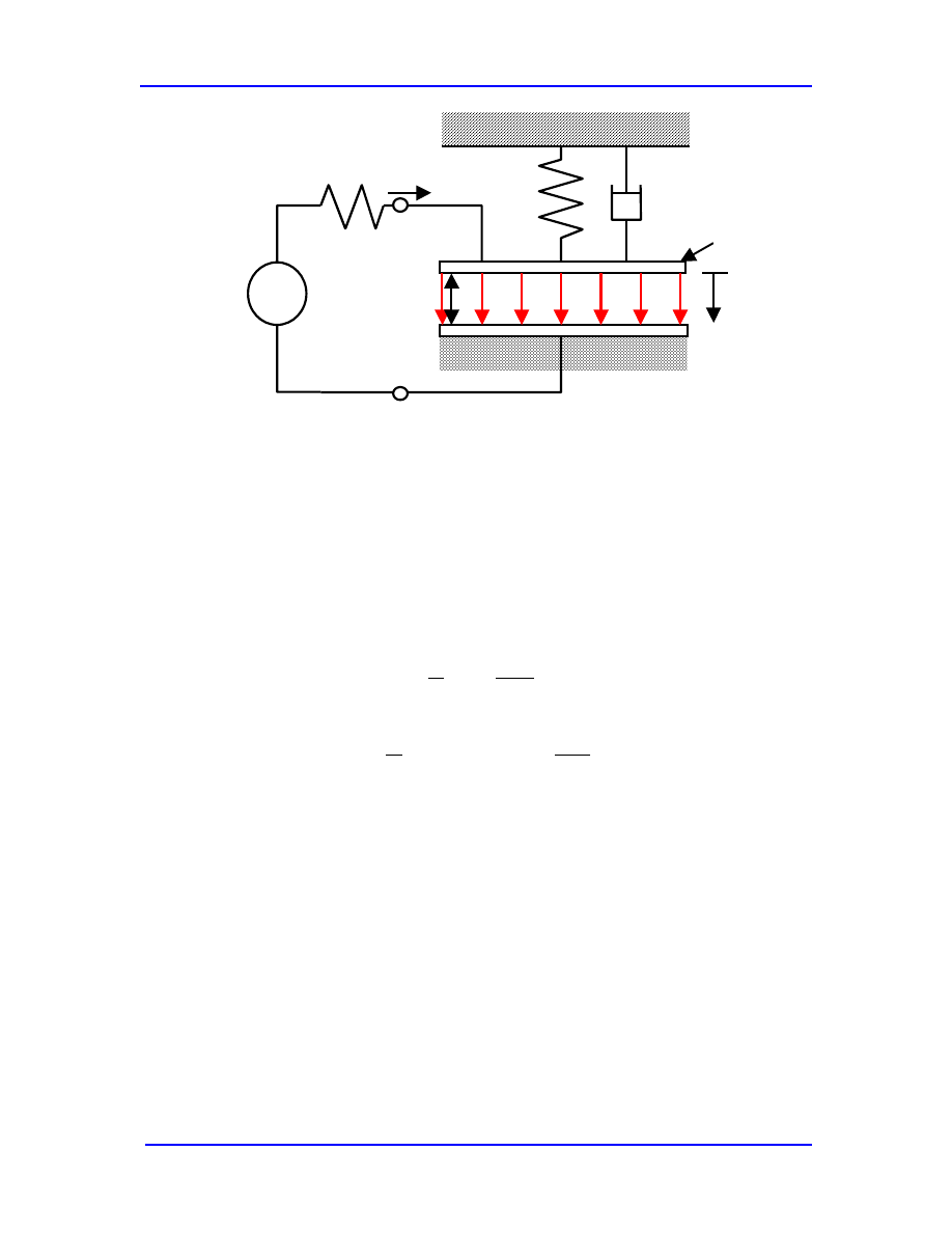
The parallel-plate electrostatic actuator of Fig. 5.1 (repeated here for convenience) is an

example of such a nonlinear system.

Nonlinear Dynamics

os, 4/22/02

EE 321, MEMS Design

Figure 6.1. Parallel plate capacitor/mechanical oscillator with electrical and mechanical

energy storage and damping. There are three mechanisms for energy
storage; electrostatic, potential energy of the mechanical spring, and kinetic
energy of the moving plate. There are therefore three independent state
variables in the description of the system.

We found the following state equations for this system

(

)

÷÷

çç

÷
ø

ç
è

−

where Q is the charge on the capacitor, g is the capacitor gap, g

is the capacitor gap

without an applied force, R is the series resistance in the electrical domain, V

is the

applied voltage, A is the area of the capacitor,

ε is the dielectric constant in the gap, m is

the mass of the moving plate, b is the damping constant, and k is the spring constant. We

see that these equations cannot be expressed in linear matrix notation.

We have solved these equations in steady state (fixed-point analysis) and found sets of

stable and unstable solutions.

Nonlinear Dynamics

os, 4/22/02

EE 321, MEMS Design

6.2

Linarization of State Equations

Fixed-point analysis naturally does not let us calculate the dynamical characteristics of a

system (although knowledge of the steady-state solutions allows us to develop intuition

about a system, and this intuition can be very valuable when trying to model dynamic

behavior). To learn more, we linearize the state equations around a fixed operating

point.

Assume that the solutions can be written as a sum of a fixed part and a small time varying

part

( )

Taylor’s theorem gives

⋅

÷÷

çç

⋅

÷÷

çç

⋅

These equations are in the form treated earlier, and we can find solutions by inverting the

appropriate matrices.

6.3

Linearization of the Electrostatic Actuator

If we know use this formalism on our electrostatic actuator example, we find

Nonlinear Dynamics

os, 4/22/02

EE 321, MEMS Design

(

)

⋅

−

⋅

÷÷

çç

÷
ø

ç
è

−

In the Lapalace domain this becomes

⋅

−

⋅

Now we can find the transfer functions of the linarized model through the customary

relation

)

(

)

(

−

In this case we have a third order transfer function, which is what we expect from a

systems with three state variables.

6.4 Softening

Spring

Even a linearized problem can be complex as we just saw for the parallel-plate

electrostatic actuator. In many instances it is a good idea to further simplify the problem

to gain insight into a specific type of behavior. As an example, we consider the softening

spring effect in parallel-plate capacitors (we briefly considered this problem earlier).

Nonlinear Dynamics

os, 4/22/02

EE 321, MEMS Design

The nonlinear characteristics of the electrostatic force creates an “electrostatic spring”

that leads to shifts of the natural frequency of microactuators

, and that can be used to

tune both the sense-mode frequency and the sensitivity of microsensors

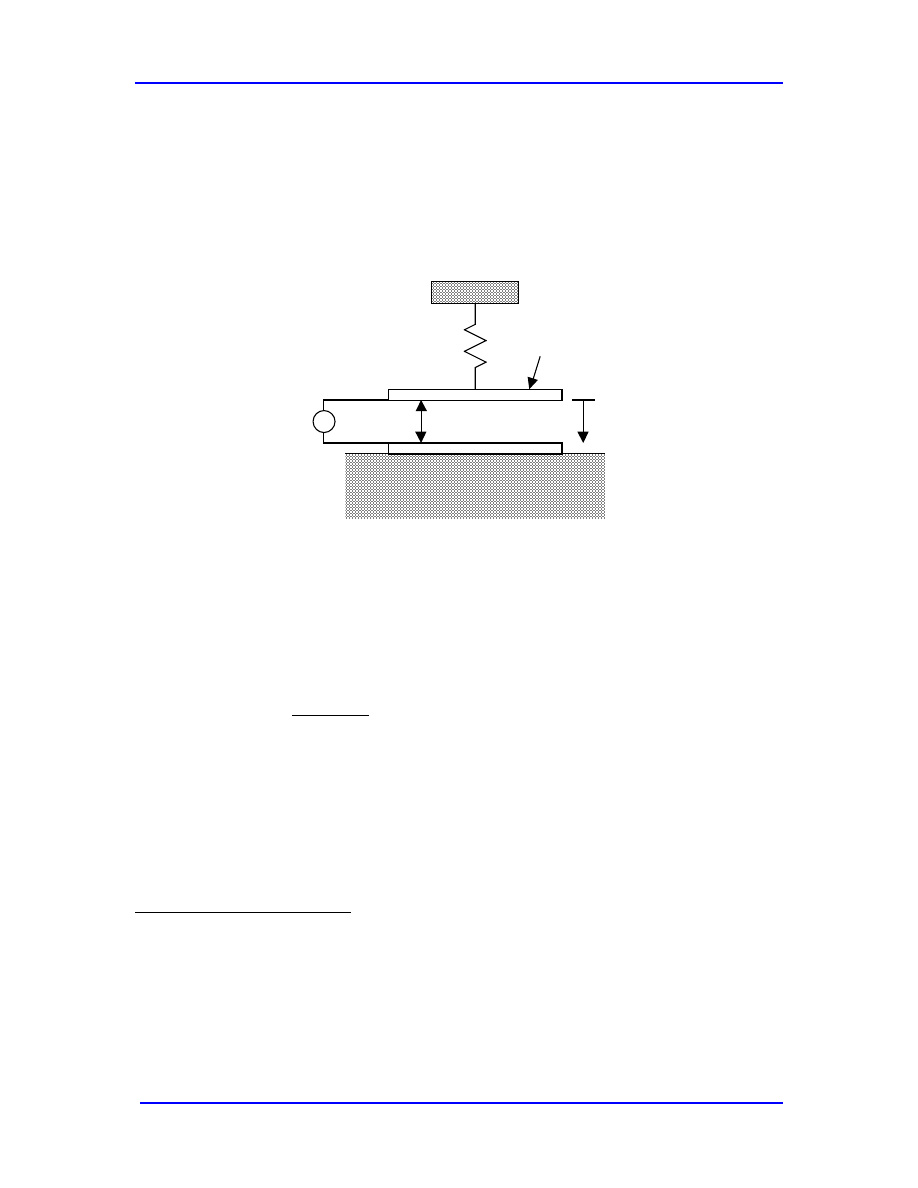
. To investigate

this phenomenon, we simplify the electrostatic as illustrated in Fig. 6.2.

Figure 6.2. Schematic drawing of parallel-plate MEMS resonator with an applied

voltage that creates an electrostatic spring that modifies the spring
constant, and therefore the natural frequency, of the resonator.

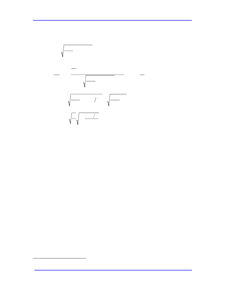
Neglecting fringing fields (not because they are not important, but because it is easy), and
the damping, we can write the force balance for the upper plate as:

)

(

−

(6.4.1)

where

is the dielectric constant and the other parameters are defined in Fig.6.2. The

nonlinear electrostatic force (the right-hand side of Eq.6.4.1) can be expanded in a Taylor
series around a nominal displacement x

Y.He, J. Marchetti, C. Gallegos, F. Maseeh, “Accurate fully-coupled natural

frequency shift of mems actuators due to voltage bias and other external forces”,
Proceedings of MEMS 99.

W.A. Clark, R.T. Howe, R. Horowitz, “Surface micromachined z-axis vibratory

rate gyroscope”, Proceedings of the Solid-Sate Sensor and Actuator Workshop, pp. 283-
287, Hilton Head, North Carolina, June 1996.

Nonlinear Dynamics

os, 4/22/02

EE 321, MEMS Design

( )( )

−

≈

−

≈

−

)

(

)

(

)

(

)

(

)

(

)

(

)

(

)

(

(6.4.2)

Inserting Eq. 6.4.2 into 6.4.1 yields:

−

÷
ø

ç
è

−

)

(

)

(

)

(

(6.4.3)

The equation is the familiar expression for a second order resonance. We see that the

mechanical spring constant is modified by the electrostatic force. This leads to a

modified resonance frequency given by:

)

(

÷
ø

ç
è

−

res

(6.4.4)

The voltage required for a specific static deflection, x

, is found from Eq. 6.4.1 (without

the time derivative term):

)

(

)

(

)

(

−

(6.4.5)

Inserted into Eq. 6.4.4, this gives:

)

(

res

−

÷÷ø

ççè

−

(6.4.6)

Solving equation 6.4.5 for the voltage, V, and maximizing, gives us the maximum

voltage, and the corresponding deflection, that the plate-spring system can support.

Applied voltages larger than this maximum will lead to spontaneous “pull-in” or “snap-

Nonlinear Dynamics

os, 4/22/02

EE 321, MEMS Design

down” to the substrate of the spring-supported plate. We’ll call this voltage (deflection)

the electrostatic instability voltage (deflection).

)

(

−

(6.4.7)

(

)

(

)

(

)

(

−

∂

(6.4.8)

)

(

snap

−

(6.4.9)

−

snap

(6.4.10)

At the instability, the resonance frequency goes to zero.

This type of “voltage controlled oscillator” has many applications. We will discuss some

of them when we go through the solutions to homework #2.

6.5

Numerical Simulations of Non-linear Systems of Equations -
Simulink

One of the simplest and most accessible tools we have for numerical simulations of non-

linear systems of equations is SIMULINK

which is a Matlab

application

. In

SIMULINK

, we program by drawing block diagrams. We choose a set of built-in

functions represented by blocks and connect them into circuits of flow diagrams.

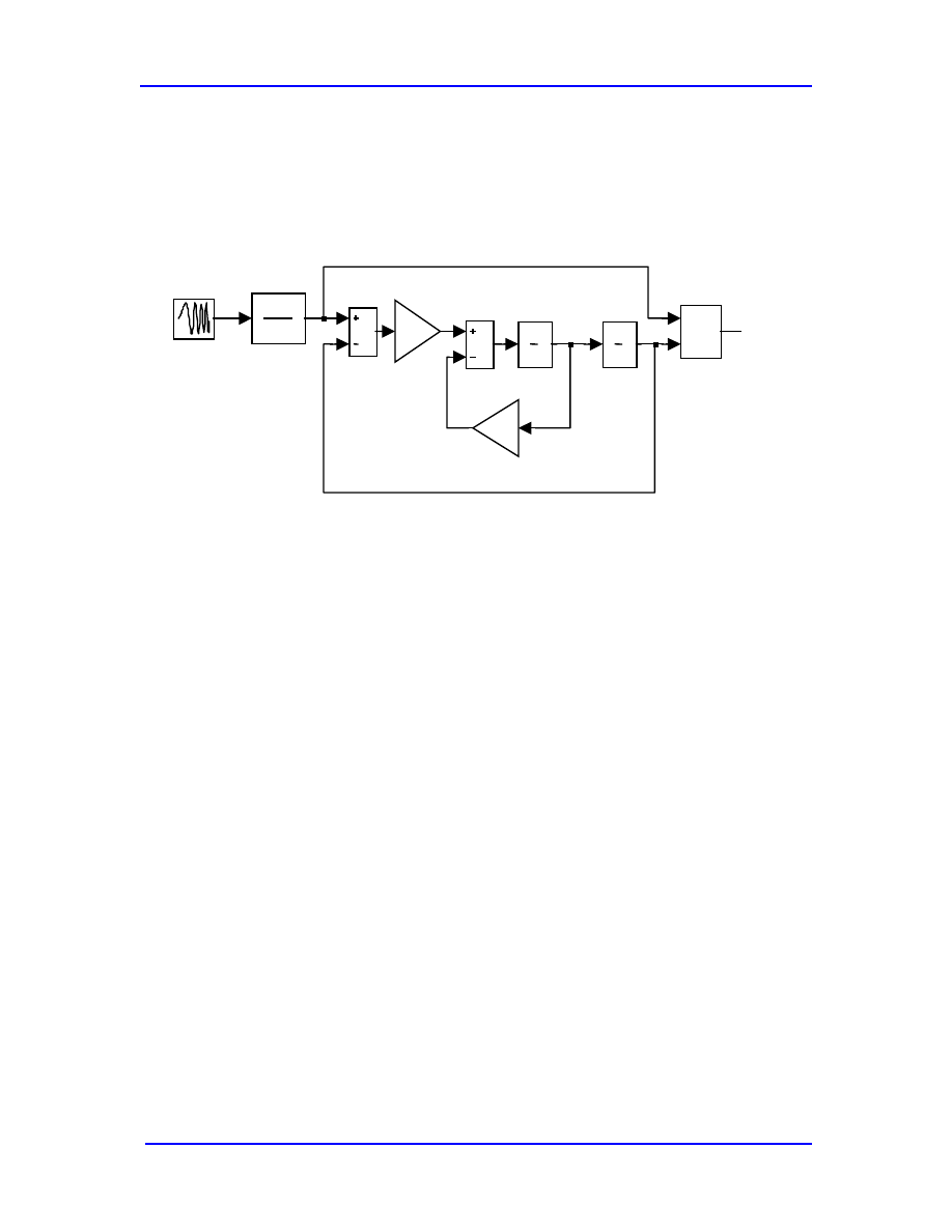
Figure 6.3 shows a simple (and familiar) example of a SIMULINK

“program”: that of a

mechanical oscillator. This particular example is linear (the input is the force on the

system), so we can solve it analytically as we have done earlier. Numerical simulations

We will use SIMULINK quite a bit in this course. If you don’t have access to it, please let me know.

Nonlinear Dynamics

os, 4/22/02

EE 321, MEMS Design

therefore add very little in this specific case, but adding non-linearities and other

complexities doesn’t make the

x2dot

Mux

x1 & x2

s+10

wn^2

Chirp Signal

Actual

Position

2*0.2

2*zeta*wn

Figure 6.3. SIMULINK® “program” of a mechanical oscillator.

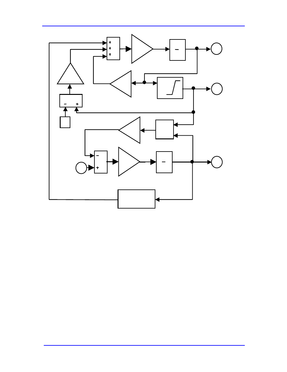
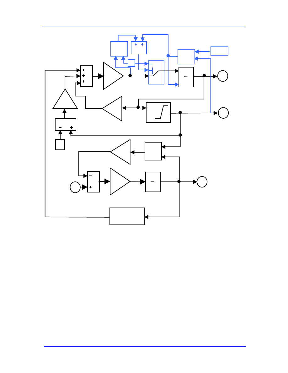
More in-depth treatments of the electrostatic actuator are shown in Figure 6.4 and 6.5.

Nonlinear Dynamics

os, 4/22/02

EE 321, MEMS Design

Charge

1/s

Position

1/R

1/(eA)

Electrostatic
force

-1/m

Velocity

g_dot

/(2*

ε*A)

Figure 6.4. Simulink model of electrostatic actuator driven by a voltage source with a

finite series resistance.

Nonlinear Dynamics

os, 4/22/02

EE 321, MEMS Design

Charge

1/s

Position

1/R

1/(eA)

Electrostatic
force

-1/m

Velocity

g_dot

/(2*

ε*A)

min

g>g

min

Figure 6.5. Simulink model for simulating pull-in effects in electrostatic actuators .

These examples illustrate the strengths and weaknesses of numerical modeling with

Simulink. On the positive side, we can model very complex systems that are not

tractable analytically. Many common nonlinear phenomena in MEMS, including

actuators with hysteresis and stiffening springs, can be simulated. The results are,

however, not better than the component models we are using.

Wyszukiwarka

Podobne podstrony:
06. Klasyfikacja wpływów dynamicznych, EGZAMIN INZYNIERSKI
20 Linearyzacja dynamiczna twierdzenie Charleta Levine Marino
Odrzucenie skargi kasacyjnej Tarno JP PP 2005 06 33, Prawo
20 Linearyzacja dynamiczna twierdzenie Charleta Levine Marino
A Novel Switch mode DC to AC Inverter With Non linear Robust Control
Chang S Y A Non linear elliptic equations in conformal geometry (EMS, 2004)(ISBN 303719006X)(O)(100s
Linear and non Linear SR 2012
PP MEMS 03 Electrostatic Actuation
A Novel Switch Mode Dc To Ac Inverter With Non Linear Robust Control
06 E83 Chassis Dynamics
06 E85 Chassis Dynamics
A Comparison of Linear Vs Non Linear Models of Aversive Self Awareness, Dissociation, and Non Suicid
Non linear rheology of active particle suspensions
06 Klasyfikacja wpływów dynamicznych, charakterystyki dynamiczne konstrukcjiid 6137 pptx
78 Non Linear Circuits
PP 2008 06
Linearization of non linear state equation
06 E65 Driving Dynamics

więcej podobnych podstron