DATA SHEET

File under Discrete Semiconductors, SC17

1997 Jan 09

DISCRETE SEMICONDUCTORS

General
Appendices

1997 Jan 09

2

Philips Semiconductors

Appendices

General

THE MAGNETORESISTIVE EFFECT

Magnetoresistive sensors make use of the fact that the
electrical resistance

ρ

of certain ferromagnetic alloys is

influenced by external fields. This solid-state
magnetoresistive effect, or anisotropic
magnetoresistance, can be easily realized using thin film
technology, so lends itself to sensor applications.

Resistance

- field relation

The specific resistance

ρ

of anisotropic ferromagnetic

metals depends on the angle

Θ

between the internal

magnetization M and the current I, according to:

ρ(Θ) = ρ

⊥

+ (ρ

⊥

− ρ

||

)

cos

2

Θ

(1)

where

ρ

⊥

and

ρ

||

are the resistivities perpendicular and

parallel to M. The quotient

(ρ

⊥

− ρ

||

)/ρ

⊥

= ∆ρ/ρ

is called the magnetoresistive effect and may amount to
several percent.

Sensors are always made from ferromagnetic thin films
as this has two major advantages over bulk material: the
resistance is high and the anisotropy can be made
uniaxial. The ferromagnetic layer behaves like a single
domain and has one distinguished direction of
magnetization in its plane called the easy axis (e.a.),
which is the direction of magnetization without external
field influence.

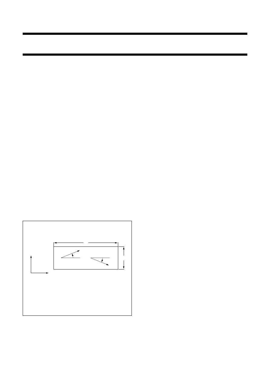
Fig.1 Geometry of a simple sensor.

handbook, halfpage

y

x

L

M

Ι

MBH616

ϕ

W

ϑ

Figure 1 shows the geometry of a simple sensor where
the thickness (t) is much smaller than the width (w) which
is in turn, less than the length (l) (i.e. t « w ‹ l). With the
current (I) flowing in the x-direction (i.e.

θ

= 0 or

Θ

=

φ

)

then the following equation can be obtained from
equation 1:
R = R

0

+ ∆

R cos

2

φ

(2)

and with a constant current

Ι

, the voltage drop in the

x-direction U

x

becomes:

U

x

=

ρ

⊥

Ι

(3)

Besides this voltage, which is directly allied to the
resistance variation, there is a voltage in the y-direction,
U

y

, given by:

U

y

= ρ

⊥

Ι

(4)

This is called the planar or pseudo Hall effect; it
resembles the normal or transverse Hall effect but has a
physically different origin.
All sensor signals are determined by the angle

φ

between

the magnetization M and the ‘length’ axis and, as M
rotates under the influence of external fields, these
external fields thus directly determine sensor signals. We
can assume that the sensor is manufactured such that the
e.a. is in the x-direction so that without the influence of
external fields, M only has an x-component
(

φ

= 0˚ or 180˚).

Two energies have to be introduced when M is rotated by
external magnetic fields: the anisotropy energy and the
demagnetizing energy. The anisotropy energy E

k

, is given

by the crystal anisotropy field H

k

, which depends on the

material and processes used in manufacture. The
demagnetizing energy E

d

or form anisotropy depends on

the geometry and this is generally a rather complex
relationship, apart from ellipsoids where a uniform
demagnetizing field H

d

may be introduced. In this case,

for the sensor set-up in Fig.1.

(5)

where the demagnetizing factor N

−

t/w, the saturation

magnetization M

s

≈

1 T and the induction constant

µ

0 = 4

π

-7

Vs/Am.

L

wt

------









1

∆ρ

ρ

-------









cos

2

φ

+









1

t

---

 

  ∆ρ

ρ

-------









sin

φ

cos

φ

H

d

t

w

----

M

s

µ

0

-------













≈

1997 Jan 09

3

Philips Semiconductors

Appendices

General

The field H

0

−

H

k

+ t/w(M

0

/m

0

) determines the measuring

range of a magnetoresistive sensor, as f is given by:

sin

φ =

(6)

where |H

y

|

≤

|H

0

+ H

x

| and H

x

and H

y

are the components

of the external field. In the simplest case H

x

= 0, the volt-

ages U

x

and U

y

become:

U

x

= ρ

⊥

l

(7)

U

y

= ρ

⊥

l

(8)

(Note: if H

x

= 0, then H

0

must be replaced by

H

0

+ H

x

/cos

φ

).

Neglecting the constant part in U

x

, there are two main

differences between U

x

and U

y

:

1. The magnetoresistive signal U

x

depends on the

square of H

y

/H

0

, whereas the Hall voltage U

y

is linear

for H

y

« H

0

.

2. The ratio of their maximum values is L/w; the Hall

voltage is much smaller as in most cases L » w.

Magnetization of the thin layer
The magnetic field is in reality slightly more complicated
than given in equation (6). There are two solutions for
angle

φ

:

φ

1 < 90˚ and

φ

2 > 90˚ (with

φ

1 +

φ

2 = 180˚ for H

x

= 0).

Replacing

φ

by 180˚ -

φ

has no influence on U

x

except to

change the sign of the Hall voltage and also that of most
linearized magnetoresistive sensors.
Therefore, to avoid ambiguity either a short pulse of a
proper field in the x-axis (|H

x

| > H

k

) with the correct sign

must be applied, which will switch the magnetization into
the desired state, or a stabilizing field Hst in the
x-direction can be used. With the exception of H

y

« H

0

, it

is advisable to use a stabilizing field as in this case, H

x

values are not affected by the non-ideal behaviour of the
layer or restricted by the so-called ‘blocking curve’.

The minimum value of H

st

depends on the structure of the

sensitive layer and has to be of the order of H

k

, as an

insufficient value will produce an open characteristic
(hysteresis) of the sensor. An easy axis in the y-direction
leads to a sensor of higher sensitivity, as then
H

o

= H

k

−

H

d

.

H

y

H

o

H

x

cos

φ

------------

+

--------------------------

L

wt

------









1

∆ρ

ρ

-------









1

H

y

H

0

-------













2

–













+













1

t

---

 

  ∆ρ

ρ

-------









H

y

H

0

-------













1

H

y

H

0

⁄

(

)

2

–

Linearization
As shown, the basic magnetoresistor has a square
resistance-field (R-H) dependence, so a simple
magnetoresistive element cannot be used directly for
linear field measurements. A magnetic biasing field can
be used to solve this problem, but a better solution is
linearization using barber-poles (described later).
Nevertheless plain elements are useful for applications
using strong magnetic fields which saturate the sensor,
where the actual value of the field is not being measured,
such as for angle measurement. In this case, the direction
of the magnetization is parallel to the field and the sensor
signal can be described by a cos

2

α

function.

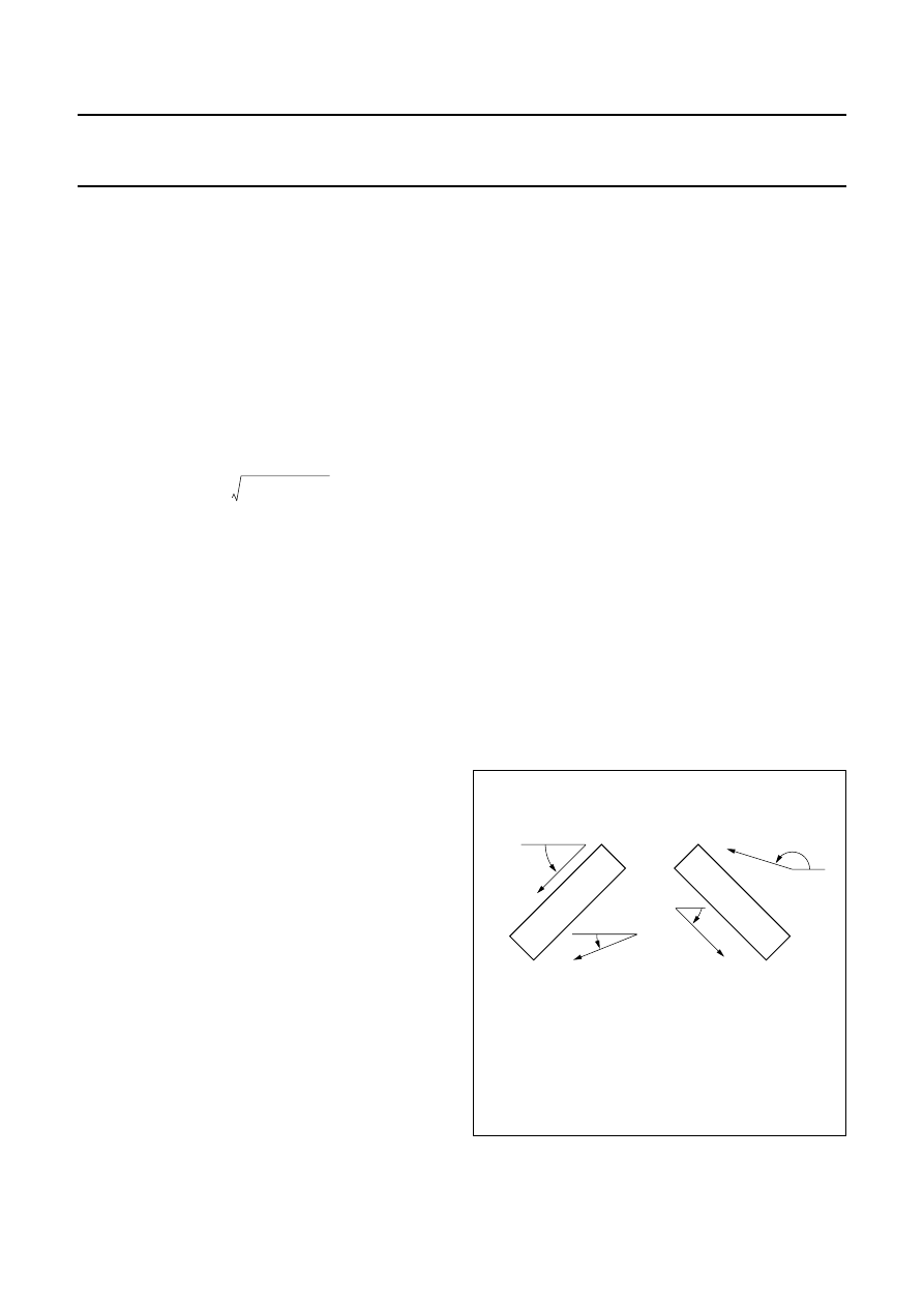
Sensors with inclined elements
Sensors can also be linearized by rotating the current
path, by using resistive elements inclined at an angle

θ

,

as shown in Fig.2. An actual device uses four inclined
resistive elements, two pairs each with opposite
inclinations, in a bridge.

The magnetic behaviour of such is pattern is more
complicated as M

o

is determined by the angle of inclination

θ

, anisotropy, demagnetization and bias field (if present).

Linearity is at its maximum for

φ

+

θ ≈

45˚, which can be

achieved through proper selection of

θ

.

A stabilization field (H

st

) in the x-direction may be

necessary for some applications, as this arrangement only
works properly in one magnetization state.

Fig.2

Current rotation by inclined elements
(current and magnetization shown in
quiescent state).

handbook, halfpage

MBH613

M0

M0

Ι

Ι

ϑ

ϑ

ϕ

ϕ

1997 Jan 09

4

Philips Semiconductors

Appendices

General

B

ARBER

-

POLE SENSORS

A number of Philips’ magnetoresistive sensors use a
‘barber-pole’ construction to linearize the R-H relationship,
incorporating slanted strips of a good conductor to rotate
the current. This type of sensor has the widest range of
linearity, smaller resistance and the least associated
distortion than any other form of linearization, and is well
suited to medium and high fields.

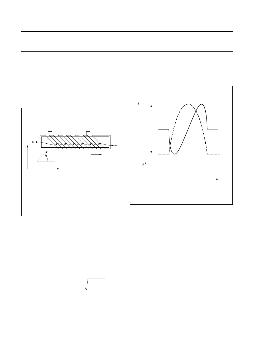
The current takes the shortest route in the high-resistivity
gaps which, as shown in Fig.3, is perpendicular to the
barber-poles. Barber-poles inclined in the opposite
direction will result in the opposite sign for the R-H
characteristic, making it extremely simple to realize a
Wheatstone bridge set-up.

The signal voltage of a Barber-pole sensor may be
calculated from the basic equation (1) with

Θ

=

φ

+ 45˚

(

θ

= + 45˚):

U

BP

= ρ

⊥

l

(9)

where a is a constant arising from the partial shorting of
the resistor, amounting to 0.25 if barber-poles and gaps
have equal widths. The characteristic is plotted in Fig.4
and it can be seen that for small values of H

y

relative to

Fig.3

Linearization of the magnetoresistive effect
with barber-poles (current and
magnetization shown in quiescent state).

handbook, halfpage

Magnetization

Barber pole

Permalloy

Ι

Ι

y

+

Ι

−

x

ϑ

,,,,

,,,,

,,,,

,,,

,,,

,,,

,,,

,,,

,,,

,,,

,,,

,,,

,,

,,

,,

,,,

,,,

,,,

,,,

,,,

,,,

MBH614

L

wt

------







 α

1

1
2

---

∆ρ

ρ

-------







 ∆ρ

ρ

-------

±

H

y

H

0

------- 1

H

y

H

0

-------













2

–

+













H

0

, the R-H dependence is linear. In fact this equation

gives the same linear R-H dependence as the planar
Hall-effect sensor, but it has the magnitude of the
magnetoresistive sensor.

Barber-pole sensors require a certain magnetization
state. A bias field of several hundred A/m can be
generated by the sensing current alone, but this is not
sufficient for sensor stabilization, so can be neglected. In
most applications, an external field is applied for this
purpose.

Sensitivity
Due to the high demagnetization, in most applications
field components in the z-direction (perpendicular to the
layer plane) can be ignored. Nearly all sensors are most
sensitive to fields in the y-direction, with H

x

only having a

limited or even negligible influence.

Definition of the sensitivity S contains the signal and field
variations (DU and DH), as well as the operating voltage
U

0

(as D

U

is proportional to U

0

):

S

o

=

(10)

This definition relates DU to a unit operating voltage.

Fig.4

Calculated R-H characteristic of a
barber-pole sensor.

handbook, halfpage

MBH615

−

0.5

0

0

R0

R

∆

R

0.5

1

HY

H0

−

1

∆

U

∆

H

--------

1

U

0

-------









∆

U

U

0

∆

H

----------------









=

1997 Jan 09

5

Philips Semiconductors

Appendices

General

The highest (H

G

) and lowest (H

min

) fields detectable by

the sensor are also of significance. The measuring range
H

G

is restricted by non-linearity - if this is assumed at 5%,

an approximate value for barber-pole sensors is given by:

(11)

From this and equation (9) for signal voltage (U

BP

) for a

barber-pole sensor, the following simple relationship can

be obtained:

(12)

Other sensor types have a narrower range of linearity and
therefore a smaller useful signal.

The lowest detectable field H

min

is limited by offset, drift

and noise. The offset is nearly cancelled in a bridge circuit
and the remaining imbalance is minimized by symmetrical
design and offset trimming, with thermal noise negligible in
most applications (see section on sensor layout). Proper
film deposition and, if necessary, the introduction of a
stabilization field will eliminate magnetization switching
due to domain splitting and the introduction of ‘Barkhausen
noise’.
Sensitivity S

0

is essentially determined by the sum of the

anisotropy (H

k

), demagnetization (H

d

) and bias (H

x

) fields.

The highest sensitivity is achievable with H

x

= 0 and

H

d

« H

k

, although in this case S

0

depends purely on H

k

which is less stable than H

d

. For a permalloy with a

thickness greater than or equal to 20

µ

m, a width in

excess of 60

µ

m is required which, although possible, has

the drawback of producing a very low resistance per unit
area.
The maximum theoretical S

0

with this permalloy (at

H

k

= 250 A/m and

∆ρ/ρ

= 2.5%) is approximately:

(13)

For the same reasons, sensors with reduced sensitivity
should be realized with increased H

d

, which can be esti-

mated at a maximum for a barber-pole sensor at 40 kA/m.
A further reduction in sensitivity and a corresponding
growth in the linearity range is attained using a biasing
field. A magnetic shunt parallel to the magnetoresistor or
only having a small field component in the sensitive direc-
tion can also be employed with very high field strengths.

A high signal voltage U

x

can only be produced with a

sensor that can tolerate a high supply voltage U

o

. This

requires a high sensor resistance R with a large area A,

H

G

0.5 H

0

H

x

+

(

)

≈

H

G

S

0

0.5

∆ρ

ρ

-------









≈

S

0

(max)

10

4

–

A

m

-----

 

 

1

100

mV

V

---------









kA

m

-------









----------------

=

=

since there are limits for power dissipation and current
density. The current density in permalloy may be very high
(j > 10

6

A/cm

2

in passivation layers), but there are weak

points at the current reversal in the meander (see section
on sensor layout) and in the barber-pole material, with
five-fold increased current density.

A high resistance sensor with U

0

= 25 V and a maximum

S

0

results in a value of 2.5 x 10

-3

(A/m)

-1

for Su or, converted to flux density, S

T

= 2000 V/T.

This value is several orders of magnitude higher than for a
normal Hall effect sensor, but is valid only for a much
narrower measuring range.

Materials

There are five major criteria for a magnetoresistive
material:

•

Large magnetoresistive effect Dr/r (resulting in a high
signal to operating voltage ratio)

•

Large specific resistance r (to achieve high resistance
value over a small area)

•

Low anisotropy

•

Zero magnetostriction (to avoid influence of mechanical
stress)

•

Long-term stability.

Appropriate materials are binary and ternary alloys of Ni,
Fe and Co, of which NiFe (81/19) is probably the most
common.

Table 1 gives a comparison between some of the more
common materials, although the majority of the figures are
only approximations as the exact values depend on a
number of variables such as thickness, deposition and
post-processing.

Table 1

Comparison of magnetoresistive sensor
materials

∆ρ

is nearly independent of these factors, but r itself

increases with thickness (t

≤

40 nm) and will decrease

during annealing. Permalloys have a low H

k

and zero

magnetostriction; the addition of C

o

will increase

∆ρ/ρ

, but

Materials

ρ

(10

−

8

Ω

m)

∆ρ

/

ρ

(%)

ΙΙ

k

(

∆

/m)

NiFe 81:19

22

2.2

250

NiFe 86:14

15

3

200

NiCo 50:50

24

2.2

2500

NiCo 70:30

26

3.7

2500

CoFeB 72:8:20

86

0.07

2000

1997 Jan 09

6

Philips Semiconductors

Appendices

General

this also considerably enlarges H

k

. If a small temperature

coefficient of

∆ρ

is required, NiCo alloys are preferable.

The amorphous alloy CoFeB has a low

∆ρ/ρ

, high H

k

and

slightly worse thermal stability but due to the absence of
grain boundaries within the amorphous structure, exhibits
excellent magnetic behaviour.

APPENDIX 2: SENSOR FLIPPING

During deposition of the permalloy strip, a strong external
magnetic field is applied parallel to the strip axis. This
accentuates the inherent magnetic anisotropy of the strip
and gives them a preferred magnetization direction, so
that even in the absence of an external magnetic field, the
magnetization will always tend to align with the strips.

Providing a high level of premagnetization within the
crystal structure of the permalloy allows for two stable
premagnetization directions. When the sensor is placed in
a controlled external magnetic field opposing the internal
aligning field, the polarity of the premagnetization of the
strips can be switched or ‘flipped’ between positive and
negative magnetization directions, resulting in two stable
output characteristics.

The field required to flip the sensor magnetization (and
hence the output characteristic) depends on the
magnitude of the transverse field H

y

. The greater this field,

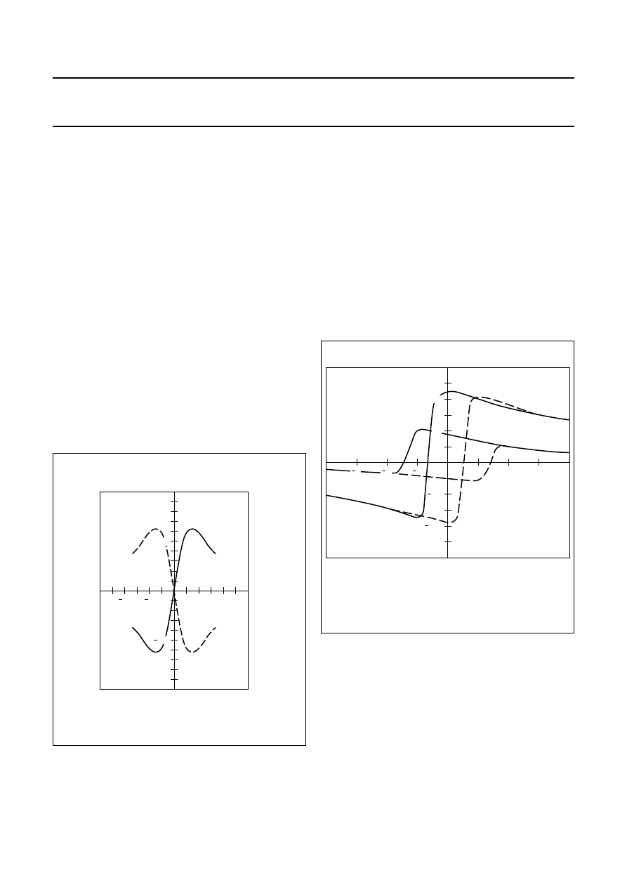
Fig.5 Sensor characteristics.

handbook, halfpage

MLC130

0

2

4

2

4

O

(mV)

H (kA/m)

y

V

10

10

reversal

of sensor

characteristics

the more the magnetization rotates towards 90˚ and
therefore it becomes easier to flip the sensor into the
corresponding stable position in the ‘-x’ direction. This
means that a smaller -H

x

field is sufficient to cause the

flipping action

As can be seen in Fig.6, for low transverse field strengths
(0.5 kA/m) the sensor characteristic is stable for all positive
values of H

x

, and a reverse field of approximately 1 kA/m

is required to flip the sensor. However at higher values of
H

y

(2 kA/m), the sensor will also flip for smaller values of

H

x

(at 0.5 kA/m). Also illustrated in this figure is a

noticeable hysteresis effect; it also shows that as the
permalloy strips do not flip at the same rate, the flipping
action is not instantaneous.

The sensitivity of the sensor reduces as the auxiliary field
H

x

increases, which can be seen in Fig.6 and more clearly

in Fig.7. This is because the moment imposed on the
magnetization by H

x

directly opposes that of H

y

, resulting

in a reduction in the degree of bridge imbalance and hence
the output signal for a given value of H

y

.

Fig.6

Sensor output ‘V

o

’ as a function of the

auxiliary field H

x

.

MLC131

0

1

2

3

1

O

(mV)

H (kA/m)

x

H =

2 kA/m

y

0.5 kA/m

V

50

100

100

50

2

3

1997 Jan 09

7

Philips Semiconductors

Appendices

General

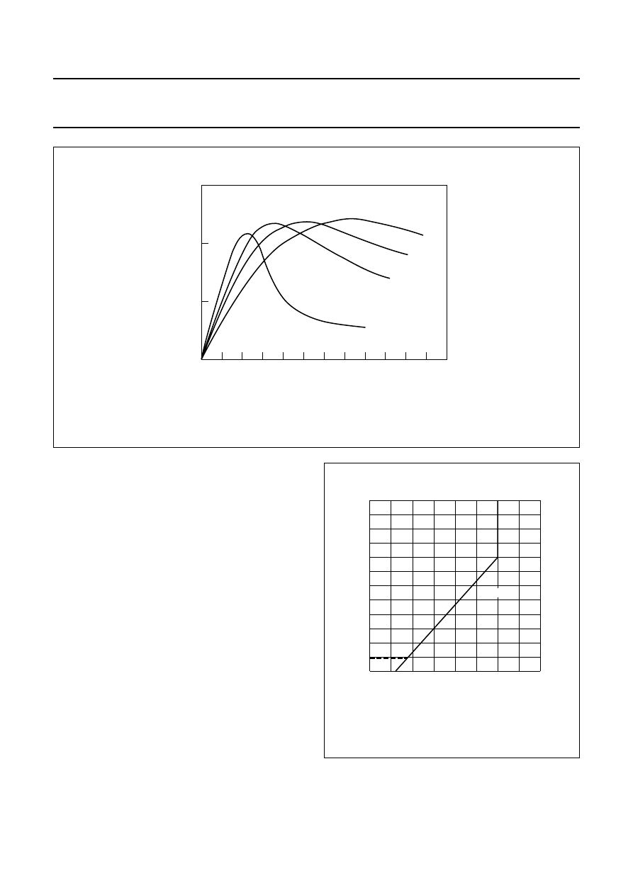
Fig.7 Sensor output ‘V

o

’ as a function of the transverse field H

y

.

handbook, full pagewidth

MLC132

0

2

4

6

8

10

12

O

(mV)

H (kA/m)

y

H =

4 kA/m

x

2 kA/m

1 kA/m

0

V

100

150

50

A Safe Operating ARea (SOAR) can be determined for
magnetoresistive sensors, within which the sensor will not
flip, depending on a number of factors. The higher the
auxiliary field, the more tolerant the sensor becomes to
external disturbing fields (H

d

) and with an H

x

of 3 kA/m or

greater, the sensor is stabilized for all disturbing fields as
long as it does not irreversibly demagnetize the sensor. If
Hd is negative and much larger than the stabilising field H

x

,

the sensor will flip. This effect is reversible, with the sensor
returning to the normal operating mode if H

d

again

becomes negligible (see Fig.8). However the higher H

x

,

the greater the reduction in sensor sensitivity and so it is
generally recommended to have a minimum auxiliary field
that ensures stable operation, generally around 1 kA/m.
The SOAR can also be extended for low values of H

x

as

long as the transverse field is less than 1 kA/m. It is also
recommended to apply a large positive auxiliary field
before first using the sensor, which erases any residual
hysteresis

Fig.8

SOAR of a KMZ10B sensor as a function of
auxiliary field ‘H

x

’ (MLC133).

handbook, halfpage

0

1

2

4

12

0

4

8

MLC133

3

Hd

(kA/m)

H (kA/m)

x

,,,,,,

,,,,,,

,,,,,,

,,,,,,

,,,,,,

,,,,,,

,,,,,,

I

II

SOAR

1997 Jan 09

8

Philips Semiconductors

Appendices

General

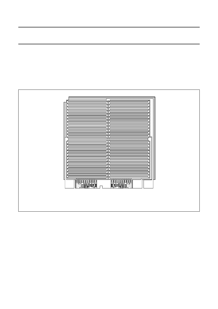
APPENDIX 3: SENSOR LAYOUT

In Philips’ magnetoresistive sensors, the permalloy strips
are formed into a meander pattern on the silicon substrate.
With the KMZ10 (see Fig.9) and KMZ51 series, four
barber-pole permalloy strips are used while the KMZ41
series has simple elements. The patterns used are
different for these three families of sensors in every case,

the elements are linked in the same fashion to form the
four arms of a Wheatstone bridge. The meander pattern
used in the KMZ51 is more sophisticated and also includes
integrated compensation and flipping coils (see chapter on
weak fields); the KMZ41 is described in more detail in the
chapter on angle measurement.

Fig.9 KMZ10 chip structure.

handbook, full pagewidth

MBC930

,,,,,

,,,,,

,,,,,

,,,,,

,,,,,

,,,,,

,,,,,

,,,,,

,,,,,

,,,,,

,,,,,

,,,,,

,,,,,

,,,,,

,,,,,

,,,,,

,,,,,

,,,,,

,,,,,

,,,,,

,,,,,

,,,,,

,,,,,

,,,,,

,,,,,

,,,,,,

,,,,,,

,,,,,,

,,,,,,

,,,,,,

,,,,,,

,,,,,,

,,,,,,

,,,,,,

,,,,,,

,,,,,,

,,,,,,

,,,,,

,,,,,,

,,,,,,

,,,,,,

,,,,,,

,,,,,,

,,,,,,

,,,,,,

,,,,,,

,,,,,,

,,,,,,

,,,,,,

,,,,,,

,,,,,,

,,,,,,

1997 Jan 09

9

Philips Semiconductors

Appendices

General

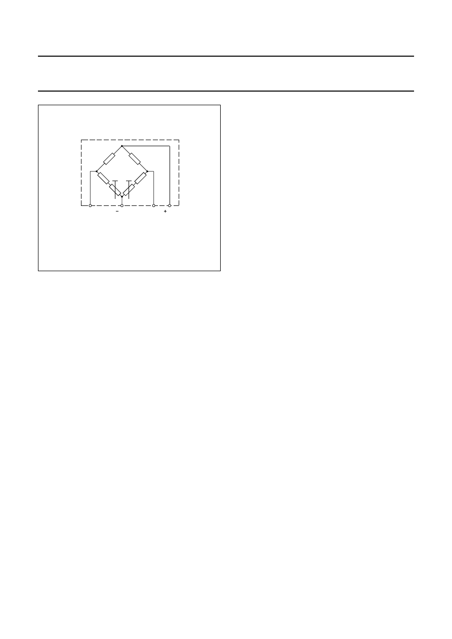
Fig.10 KMZ10 and KMZ11 bridge configuration.

handbook, halfpage

MLC129

2

1

GND

VO

VCC

VO

RT

RT

3

4

In one pair of diagonally opposed elements the
barber-poles are at +45˚ to the strip axis, with the second
pair at

−

45˚. A resistance increase in one pair of elements

due to an external magnetic field is matched by an equal
decrease in resistance of the second pair. The resulting
bridge imbalance is then a linear function of the amplitude
of the external magnetic field in the plane of the permalloy
strips normal to the strip axis.

This layout largely eliminates the effects of ambient
variations (e.g. temperature) on the individual elements
and also magnifies the degree of bridge imbalance,
increasing sensitivity.

Fig.10 indicates two further trimming resistors (R

T

) which

allow the sensors electrical offset to be trimmed down to
zero during the production process.