
2000 Sep 06
DISCRETE SEMICONDUCTORS
General
Magnetoresistive sensors for
magnetic field measurement
2000 Sep 06
2
Philips Semiconductors
Magnetoresistive sensors for
magnetic field measurement
General
CONTENTS
General field measurement
•
Operating principles
•
Philips magnetoresistive sensors
•
Flipping
•
Effect of temperature on behaviour
•
Using magnetoresistive sensors
•
Further information for advanced users
•
Appendix 1: The magnetoresistive effect
•
Appendix 2: Sensor flipping
•
Appendix 3: Sensor layout.
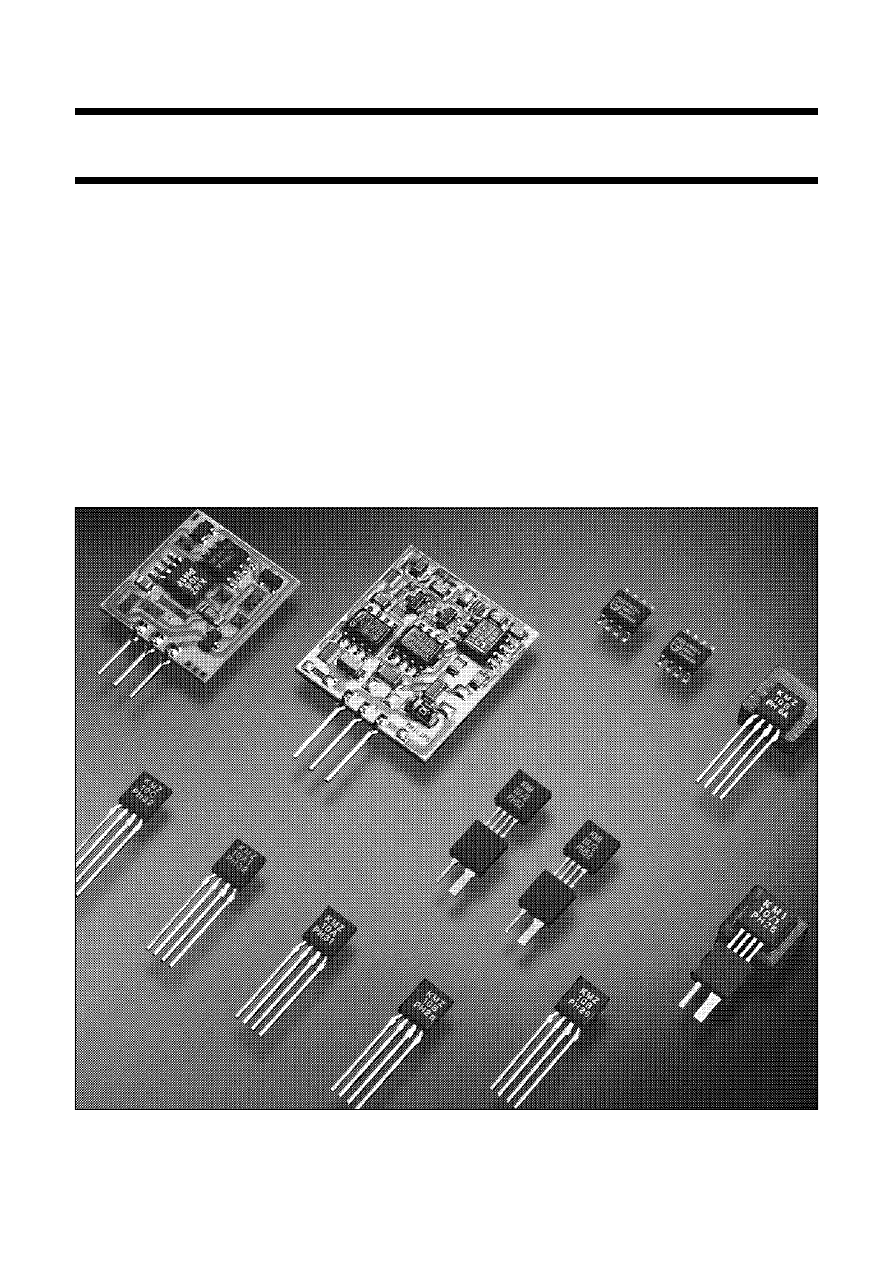
Fig.1 Philips magnetoresistive sensors.
2000 Sep 06
3
Philips Semiconductors
Magnetoresistive sensors for
magnetic field measurement
General
The KMZ range of magnetoresistive sensors is
characterized by high sensitivity in the detection of
magnetic fields, a wide operating temperature range, a low
and stable offset and low sensitivity to mechanical stress.
They therefore provide an excellent means of measuring
both linear and angular displacement under extreme
environmental conditions, because their very high
sensitivity means that a fairly small movement of actuating
components in, for example, cars or machinery (gear
wheels, metal rods, cogs, cams, etc.) can create
measurable changes in magnetic field. Other applications
for magnetoresistive sensors include rotational speed
measurement and current measurement.
Examples where their properties can be put to good effect
can be found in automotive applications, such as wheel
speed sensors for ABS and motor management systems
and position sensors for chassis position, throttle and
pedal position measurement. Other examples include
instrumentation and control equipment, which often
require position sensors capable of detecting
displacements in the region of tenths of a millimetre (or
even less), and in electronic ignition systems, which must
be able to determine the angular position of an internal
combustion engine with great accuracy.
Finally, because of their high sensitivity, magnetoresistive
sensors can measure very weak magnetic fields and are
thus ideal for application in electronic compasses, earth
field correction and traffic detection.
If the KMZ sensors are to be used to maximum advantage,
however, it is important to have a clear understanding of
their operating principles and characteristics, and how
their behaviour may be affected by external influences and
by their magnetic history.
Operating principles
Magnetoresistive (MR) sensors make use of the
magnetoresistive effect, the property of a current-carrying
magnetic material to change its resistivity in the presence
of an external magnetic field (the common units used for
magnetic fields are given in Table 1).
Table 1
Common magnetic units
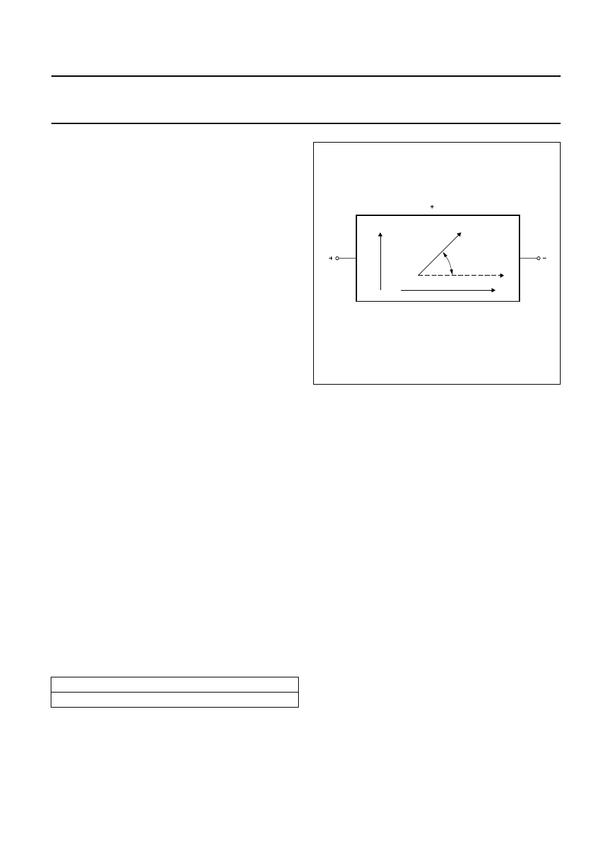
The basic operating principle of an MR sensor is shown in
Fig.2.
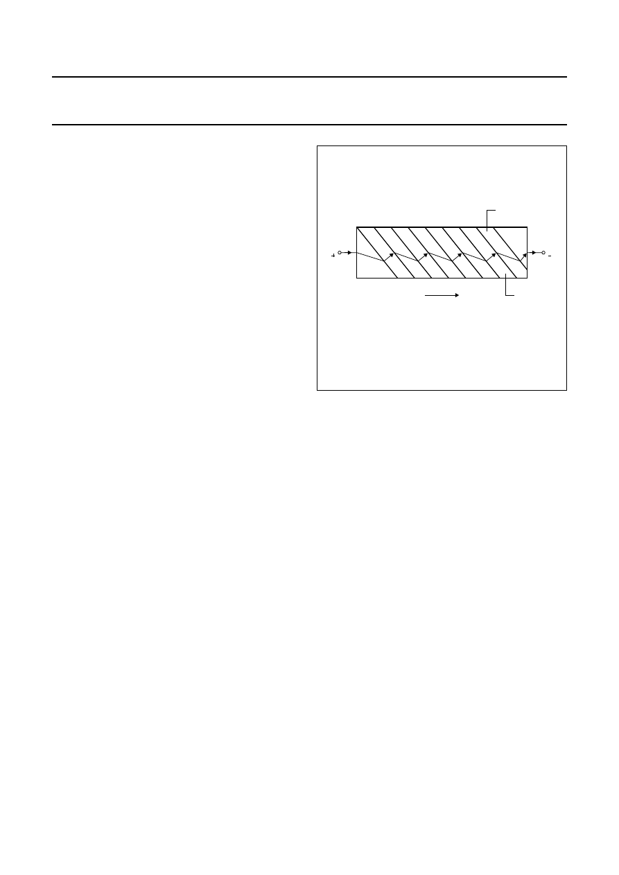
Figure 2 shows a strip of ferromagnetic material, called
permalloy (20% Fe, 80% Ni). Assume that, when no
external magnetic field is present, the permalloy has an
internal magnetization vector parallel to the current flow
(shown to flow through the permalloy from left to right).
If an external magnetic field H is applied, parallel to the
plane of the permalloy but perpendicular to the current
flow, the internal magnetization vector of the permalloy will
rotate around an angle
α
. As a result, the resistance of R
of the permalloy will change as a function of the rotation
angle
α
, as given by:
(1)
R
o
and
∆
R
o
are material parameters and to achieve
optimum sensor characteristics Philips use Ni19Fe81,
which has a high R
o
value and low magnetostriction. With
this material,
∆
R
o
is of the order of 3%. For more
information on materials, see Appendix 1.
It is obvious from this quadratic equation, that the
resistance/magnetic field characteristic is non-linear and in
addition, each value of R is not necessarily associated
with a unique value of H (see Fig.3). For more details on
the essentials of the magnetoresistive effect, please refer
to the Section “Further information for advanced users”
later in this chapter or Appendix 1, which examines the MR
effect in detail.
1 kA/m = 1.25 mTesla (in air)
1 mT = 10 Gauss
Fig.2 The magnetoresistive effect in permalloy.
handbook, halfpage
MLC127
I
Magnetization
Permalloy
H
Current
α
R = R
∆
R cos
α
2
0
0
R
R
O
∆
R
O
cos
2
α
+
=
2000 Sep 06
4
Philips Semiconductors
Magnetoresistive sensors for
magnetic field measurement
General
In this basic form, the MR effect can be used effectively for
angular measurement and some rotational speed
measurements, which do not require linearization of the
sensor characteristic.
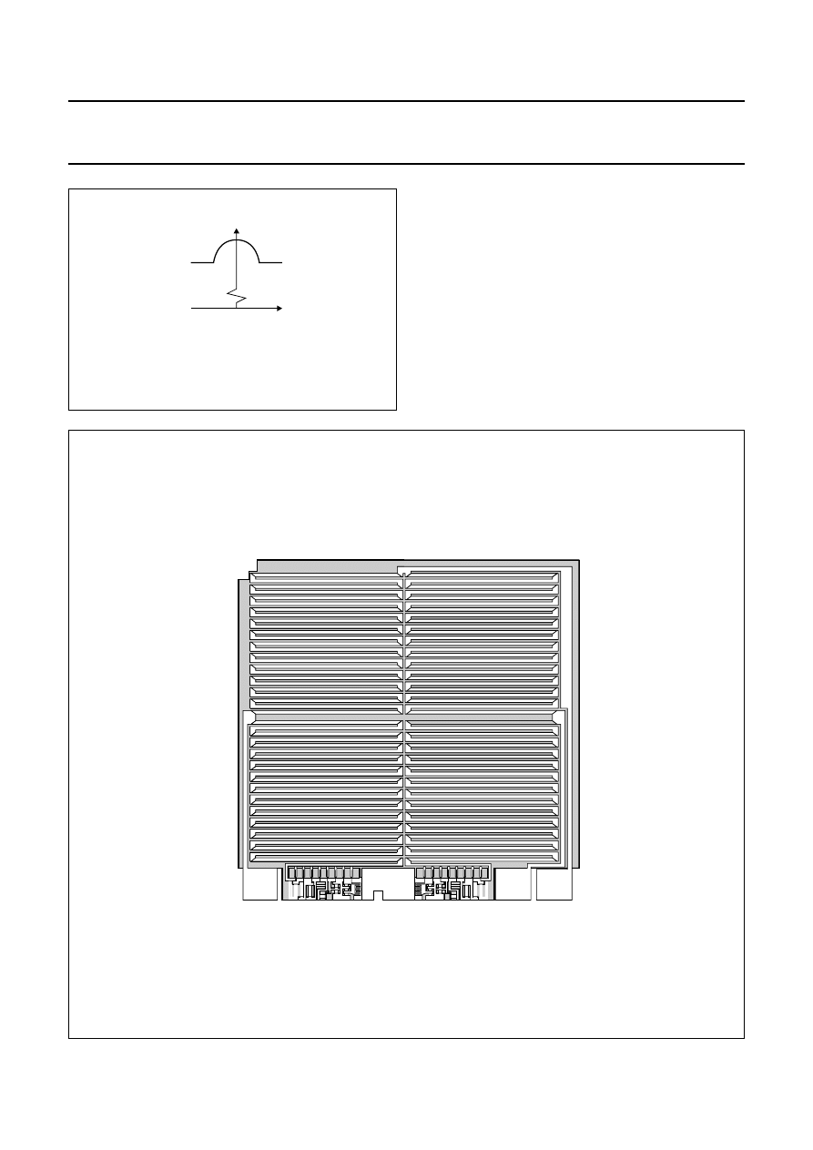
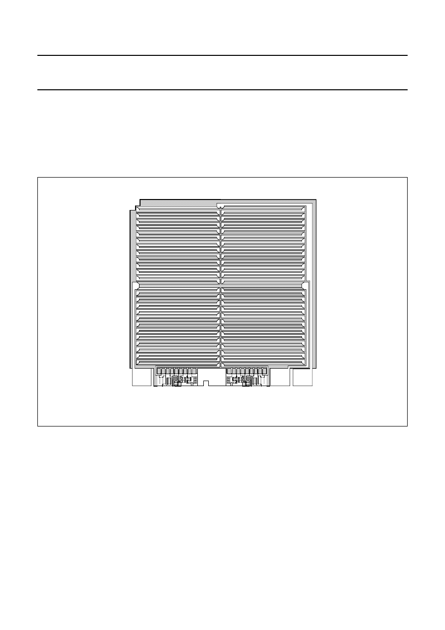
In the KMZ series of sensors, four permalloy strips are
arranged in a meander fashion on the silicon (Fig.4 shows
one example, of the pattern on a KMZ10). They are
connected in a Wheatstone bridge configuration, which
has a number of advantages:
•
Reduction of temperature drift
•
Doubling of the signal output
•
The sensor can be aligned at the factory.
Fig.3
The resistance of the permalloy as a
function of the external field.
handbook, halfpage
MLC128
H
R
Fig.4 KMZ10 chip structure.
handbook, full pagewidth
MBC930
,,,,,
,,,,,
,,,,,
,,,,,
,,,,,
,,,,,
,,,,,
,,,,,
,,,,,
,,,,,
,,,,,
,,,,,
,,,,,
,,,,,
,,,,,
,,,,,
,,,,,
,,,,,
,,,,,
,,,,,
,,,,,
,,,,,
,,,,,
,,,,,
,,,,,
,,,,,,
,,,,,,
,,,,,,
,,,,,,
,,,,,,
,,,,,,
,,,,,,
,,,,,,
,,,,,,
,,,,,,
,,,,,,
,,,,,,
,,,,,
,,,,,,
,,,,,,
,,,,,,
,,,,,,
,,,,,,
,,,,,,
,,,,,,
,,,,,,
,,,,,,
,,,,,,
,,,,,,
,,,,,,
,,,,,,
,,,,,,
2000 Sep 06
5
Philips Semiconductors
Magnetoresistive sensors for
magnetic field measurement
General
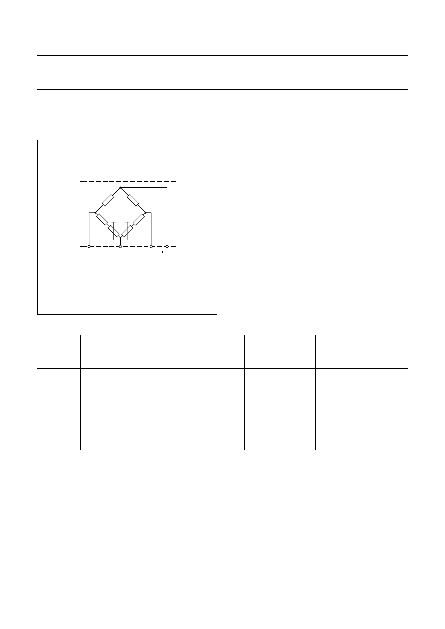
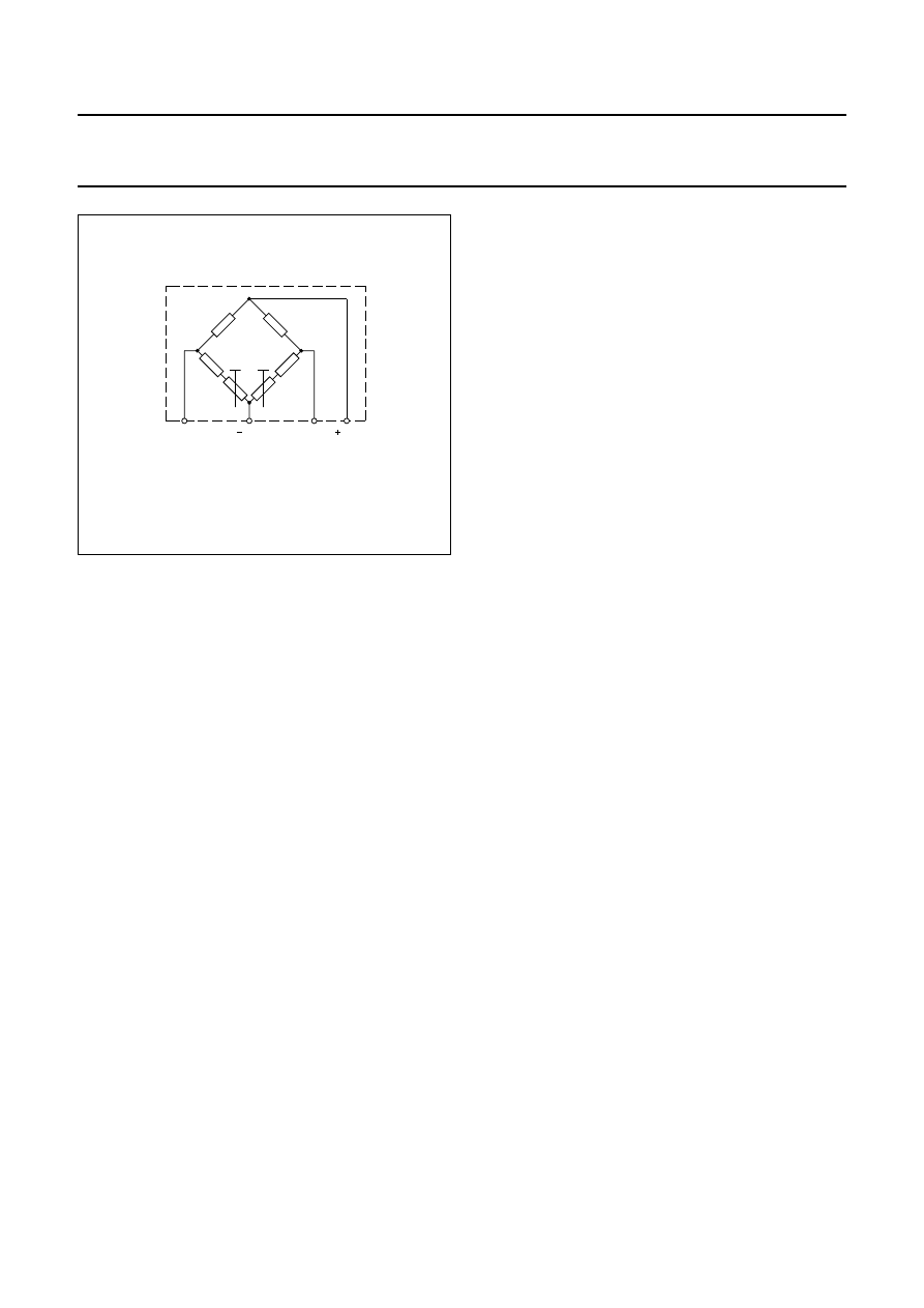
Two further resistors, R
T
, are included, as shown in Fig.5.
These are for trimming sensor offset down to (almost) zero
during the production process.
For some applications however, the MR effect can be used
to its best advantage when the sensor output
characteristic has been linearized. These applications
include:
•
Weak field measurements, such as compass
applications and traffic detection;
•
Current measurement; and
•
Rotational speed measurement.
For an explanation of how the characteristic is linearized,
please refer to the Section “Further information for
advanced users” later in this chapter.
Philips magnetoresistive sensors
Based on the principles described, Philips has a family of
basic magnetoresistive sensors. The main characteristics
of the KMZ sensors are given in Table 2.
Fig.5
Bridge configuration with offset trimmed to
zero, by resistors R
T
.
handbook, halfpage
MLC129
2
1
GND
VO
VCC
VO
RT
RT
3
4
Table 2
Main characteristics of Philips sensors
Notes
1. In air, 1 kA/m corresponds to 1.25 mT.
2. Data given for operation with switched auxiliary field.
SENSOR
TYPE
PACKAGE
FIELD
RANGE
(kA/m)
(1)
V
CC
(V)
SENSITIVITY
R
bridge
(k
Ω
)
LINEARIZE
MR
EFFECT
APPLICATION
EXAMPLES
KMZ10A
SOT195
−
0.5 to +0.5
≤
9
16.0
1.2
Yes
compass, navigation, metal
detection, traffic control
KMZ10A1
(2)
SOT195
−
0.05 to +0.05
≤
9
22.0
1.3
Yes
KMZ10B
SOT195
−
2.0 to +2.0
≤
12
4.0
2.1
Yes
current measurement,
angular and linear position,
reference mark detection,
wheel speed
KMZ10C
SOT195
−
7.5 to +7.5
≤
10
1.5
1.4
Yes
KMZ51
SO8
−
0.2 to +0.2
≤
8
16.0
2.0
Yes
compass, navigation, metal
detection, traffic control
KMZ52
SO16
−
0.2 to +0.2
≤
8
16.0
2.0
Yes
mV V
⁄
(
)
kA m
⁄
(
)
---------------------
2000 Sep 06
6
Philips Semiconductors
Magnetoresistive sensors for
magnetic field measurement
General
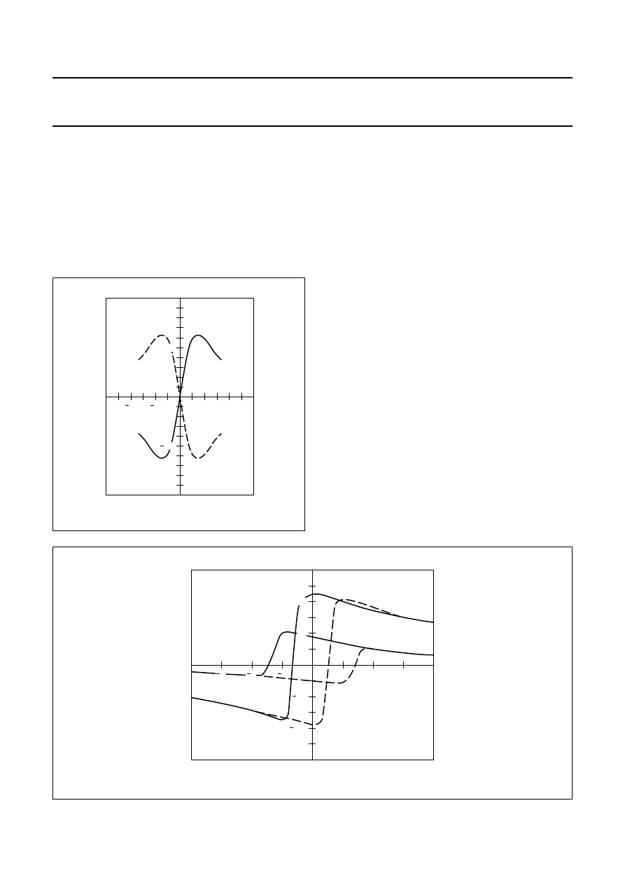
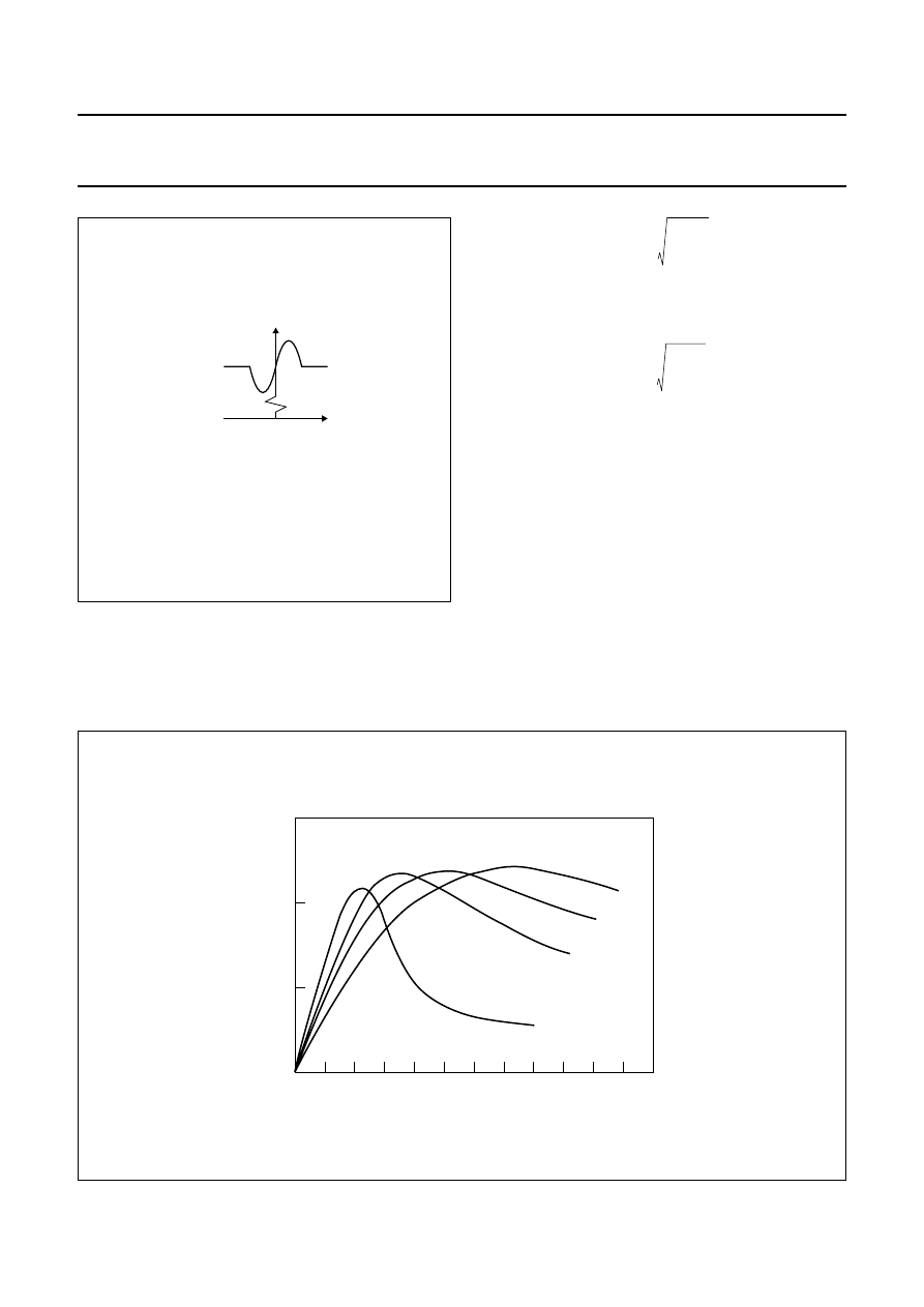
Flipping
The internal magnetization of the sensor strips has two
stable positions. So, if for any reason the sensor is
influenced by a powerful magnetic field opposing the
internal aligning field, the magnetization may flip from one
position to the other, and the strips become magnetized in
the opposite direction (from, for example, the ‘+x’ to the
‘
−
x’ direction). As demonstrated in Fig.6, this can lead to
drastic changes in sensor characteristics.
The field (e.g. ‘
−
H
x
’) needed to flip the sensor
magnetization, and hence the characteristic, depends on
the magnitude of the transverse field ‘H
y
’: the greater the
field ‘H
y
’, the smaller the field ‘
−
H
x
’. This follows naturally,
since the greater the field ‘H
y
’, the closer the
magnetization's rotation approaches 90
°
, and hence the
easier it will be to flip it into a corresponding stable position
in the ‘
−
x’ direction.
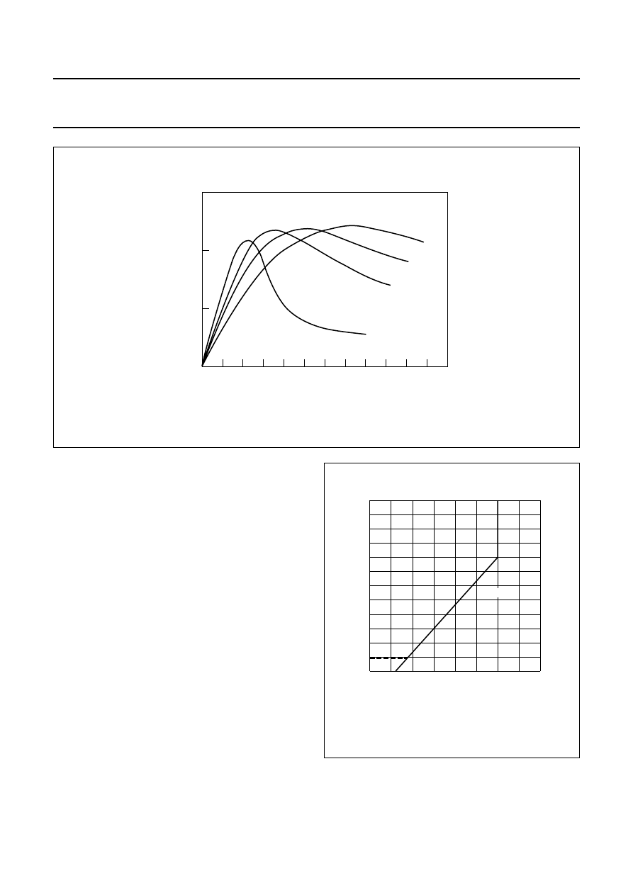
Looking at the curve in Fig.7 where H
y
= 0.5 kA/m, for
such a low transverse field the sensor characteristic is
stable for all positive values of H
x
and a reverse field of
≈
1 kA/m is required before flipping occurs. At H
y
= 2 kA/m
however, the sensor will flip even at smaller values of ‘H
x
’
(at approximately 0.5 kA/m).
Fig.6 Sensor characteristics.
handbook, halfpage
MLC130
0
2
4
2
4
O
(mV)
H (kA/m)
y
V
10
10
reversal
of sensor
characteristics
Fig.7 Sensor output ‘V
o
’ as a function of the auxiliary field ‘H
x
’ for several values of transverse field ‘H
y
’.
handbook, full pagewidth
MLC131
0
1
2
3
1
O
(mV)
H (kA/m)
x
H =
2 kA/m
y
0.5 kA/m
V
50
100
100
50
2
3
2000 Sep 06
7
Philips Semiconductors
Magnetoresistive sensors for
magnetic field measurement
General
Figure 7 also shows that the flipping itself is not
instantaneous, because not all the permalloy strips flip at
the same rate. In addition, it illustrates the hysteresis effect
exhibited by the sensor. For more information on sensor
flipping, see Appendix 2 of this chapter.
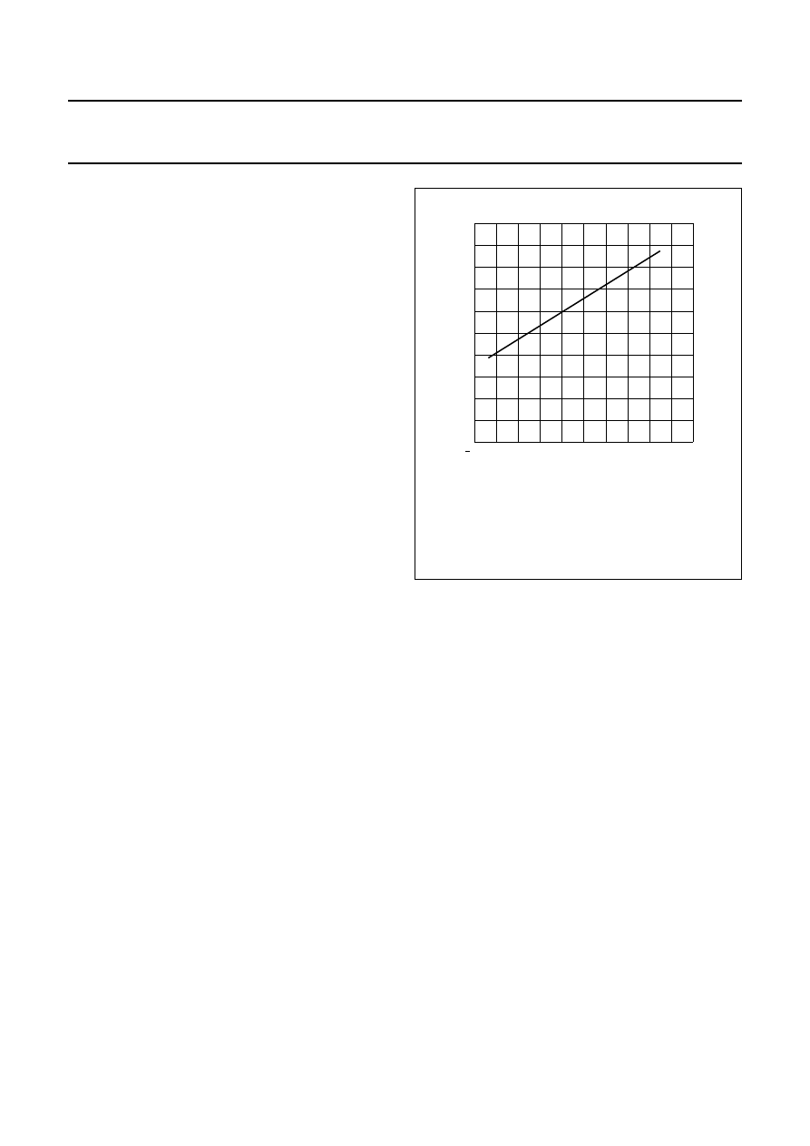
Effect of temperature on behaviour
Figure 8 shows that the bridge resistance increases
linearly with temperature, due to the bridge resistors’
temperature dependency (i.e. the permalloy) for a typical
KMZ10B sensor. The data sheets show also the spread in
this variation due to manufacturing tolerances and this
should be taken into account when incorporating the
sensors into practical circuits.
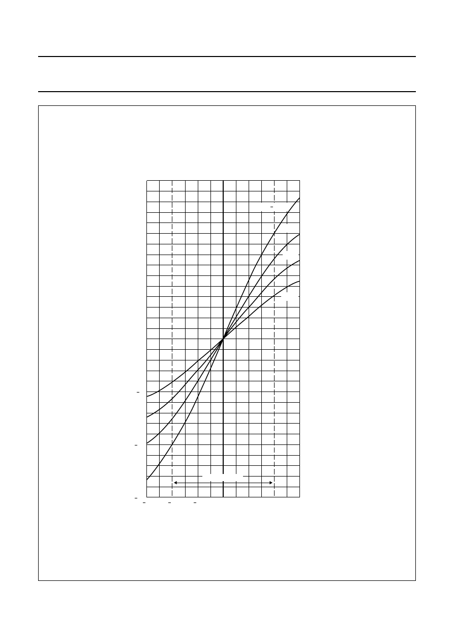
In addition to the bridge resistance, the sensitivity also
varies with temperature. This can be seen from Fig.9,
which plots output voltage against transverse field ‘H
y
’ for
various temperatures. Figure 9 shows that sensitivity falls
with increasing temperature (actual values for given for
every sensor in the datasheets). The reason for this is
rather complex and is related to the energy-band structure
of the permalloy strips.
Fig.8
Bridge resistance of a KMZ10B sensor as
a function of ambient temperature.
handbook, halfpage
40
160
3
1
MBB897
2
0
40
80
120
T ( C)
o
amb
bridge
R
(k
Ω
)
2000 Sep 06
8
Philips Semiconductors
Magnetoresistive sensors for
magnetic field measurement
General
Fig.9
Output voltage ‘V
o
’ as a fraction of the supply voltage of a KMZ10B sensor as a function of transverse field
‘H
y
’ for several temperatures.
handbook, full pagewidth
3
0
15
3
2
2
MLC134
5
10
10
5
15
0
1
1
H (kA/m)
y
VO
(mV/V)
T = 25 C
amb
o
25 C
o
75 C
o
125 C
o
operating range
2000 Sep 06
9
Philips Semiconductors
Magnetoresistive sensors for
magnetic field measurement
General
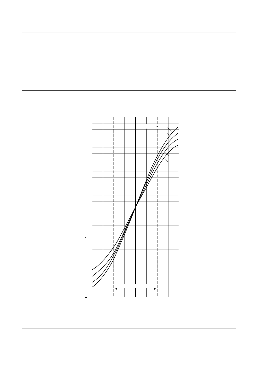
Figure 10 is similar to Fig.9, but with the sensor powered
by a constant current supply. Figure 10 shows that, in this
case, the temperature dependency of sensitivity is
significantly reduced. This is a direct result of the increase
in bridge resistance with temperature (see Fig.8), which
partly compensates the fall in sensitivity by increasing the
voltage across the bridge and hence the output voltage.
Figure 8 demonstrates therefore the advantage of
operating with constant current.
Fig.10 Output voltage ‘V
o
’ of a KMZ10B sensor as a function of transverse field ‘H
y
’ for several temperatures.
handbook, full pagewidth
0
75
4
2
MLC135
25
50
50
25
75
2
0
4
H (kA/m)
y
VO
(mV/V)
T = 25 C
amb
o
25 C
o
75 C
o
125 C
o
operating range
2000 Sep 06
10
Philips Semiconductors
Magnetoresistive sensors for
magnetic field measurement
General
Using magnetoresistive sensors
The excellent properties of the KMZ magnetoresistive
sensors, including their high sensitivity, low and stable
offset, wide operating temperature and frequency ranges
and ruggedness, make them highly suitable for use in a
wide range of automotive, industrial and other
applications. These are looked at in more detail in other
chapters in this book; some general practical points about
using MR sensors are briefly described below.
A
NALOG APPLICATION CIRCUITRY
In many magnetoresistive sensor applications where
analog signals are measured (in measuring angular
position, linear position or current measurement, for
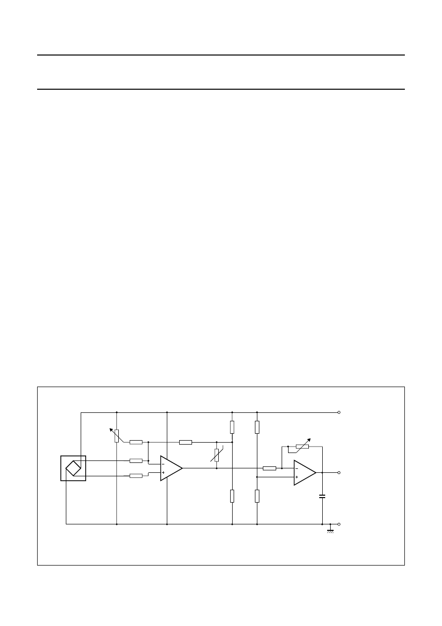
example), a good application circuit should allow for
sensor offset and sensitivity adjustment. Also, as the
sensitivity of many magnetic field sensors has a drift with
temperature, this also needs compensation. A basic circuit
is shown in Fig.11.
In the first stage, the sensor signal is pre-amplified and
offset is adjusted. After temperature effects are
compensated, final amplification and sensitivity
adjustment takes place in the last stage. This basic circuit
can be extended with additional components to meet
specific EMC requirements or can be modified to obtain
customized output characteristics (e.g. a different output
voltage range or a current output signal).
Philips magnetoresistive sensors have a linear sensitivity
drift with temperature and so a temperature sensor with
linear characteristics is required for compensation. Philips
KTY series are well suited for this purpose, as their
positive Temperature Coefficient (TC) matches well with
the negative TC of the MR sensor. The degree of
compensation can be controlled with the two resistors R7
and R8 and special op-amps, with very low offset and
temperature drift, should be used to ensure compensation
is constant over large temperature ranges.
Please refer to part 2 of this book for more information on
the KTY temperature sensors; see also the Section
“Further information for advanced users” later in this
chapter for a more detailed description of temperature
compensation using these sensors.
U
SING MAGNETORESISTIVE SENSORS WITH A COMPENSATION
COIL
For general magnetic field or current measurements it is
useful to apply the ‘null-field’ method, in which a magnetic
field (generated by a current carrying coil), equal in
magnitude but opposite in direction, is applied to the
sensor. Using this ‘feedback’ method, the current through
the coil is a direct measure of the unknown magnetic field
amplitude and it has the advantage that the sensor is being
operated at its zero point, where inaccuracies as result of
tolerances, temperature drift and slight non-linearities in
the sensor characteristics are insignificant. A detailed
discussion of this method is covered in Chapter “Weak
field measurement”.
Fig.11 Basic application circuit with temperature compensation and offset adjustment.
handbook, full pagewidth
MBH687
3
4
1
2
KMZ10B
offset
adjustment
R3
22 k
Ω
R4
14 k
Ω
R2
500 k
Ω
R1
100 k
Ω
2
3
4
1
8
R6
KTY82-210
TLC2272
R5
140 k
Ω
R7
2.4 k
Ω
R8
2.4 k
Ω
R9
33 k
Ω
R10
33 k
Ω
6
5
7
IC1
R11
22 k
Ω
R12
150 k
Ω
sensitivity
adjustment
C1
10 nF
V = 5 V
S
V = 0.2 V to 4.8 V
O
(with resistive load
greater than 10 k
Ω
)
op-amp
op-amp
2000 Sep 06
11
Philips Semiconductors
Magnetoresistive sensors for
magnetic field measurement
General
Further information for advanced users
T
HE
MR
EFFECT
In sensors employing the MR effect, the resistance of the
sensor under the influence of a magnetic field changes as
it is moved through an angle
α
as given by:
(2)
It can be shown that
(3)
and
(4)
where H
o
can be regarded as a material constant
comprising the so called demagnetizing and anisotropic
fields.
Applying equations (3) and (4) to equation (2) leads to:
(5)
(6)
which clearly shows the non-linear nature of the MR effect.
More detailed information on the derivation of the formulae
for the MR effect can be found in Appendix 1.
L
INEARIZATION
The magnetoresistive effect can be linearized by
depositing aluminium stripes (Barber poles), on top of the
permalloy strip at an angle of 45
°
to the strip axis (see
Fig.12). As aluminium has a much higher conductivity than
permalloy, the effect of the Barber poles is to rotate the
current direction through 45
°
(the current flow assumes a
‘saw-tooth’ shape), effectively changing the rotation angle
of the magnetization relative to the current from
α
to
α −
45
°
.
A Wheatstone bridge configuration is also used for
linearized applications. In one pair of diagonally opposed
elements, the Barber poles are at +45
°
to the strip axis,
while in another pair they are at
−
45
°
. A resistance
increase in one pair of elements due to an external
magnetic field is thus ‘matched’ by a decrease in
resistance of equal magnitude in the other pair.
The resulting bridge imbalance is then a linear function of
the amplitude of the external magnetic field in the plane of
the permalloy strips, normal to the strip axis.
R
R
O
∆
R
O
cos
2
α
+
=
sin
2
α
H
2
H
O
2
-------- for H
H
O
≤
=
sin
2
α
1 for H
H
O
>
=
R
R
O
∆
R
O
1
H
2
H
O
2
--------
–
for H
H
0
≤
+
=
R
R
O
for H
H
O
>
=
Fig.12 Linearization of the magnetoresistive effect.
handbook, halfpage
MLC125
,,
,,
,,
,,,
,,,
,,,
,,,,
,,,,
,,,,
,,,
,,,
,,,
,,,
,,,
,,,
I
I
Magnetization
Permalloy
Barber pole
2000 Sep 06
12
Philips Semiconductors
Magnetoresistive sensors for
magnetic field measurement
General
For sensors using Barber poles arranged at an angle of
+45
°
to the strip axis, the following expression for the
sensor characteristic can be derived (see Appendix 1 on
the MR effect):
(7)
The equation is linear where H/H
o
= 0, as shown in Fig.7.
Likewise, for sensors using Barber poles arranged at an
angle of
−
45
°
, the equation derives to:
(8)
This is the mirror image of the characteristic in Fig.7.
Hence using a Wheatstone bridge configuration ensures
the any bridge imbalance is a linear function of the
amplitude of the external magnetic field.
F
LIPPING
As described in the body of the chapter, Fig.7 shows that
flipping is not instantaneous and it also illustrates the
hysteresis effect exhibited by the sensor. This figure and
Fig.14 also shows that the sensitivity of the sensor falls
with increasing ‘H
x
’. Again, this is to be expected since the
moment imposed on the magnetization by ‘H
x
’ directly
opposes that imposed by ‘H
y
’, thereby reducing the degree
of bridge imbalance and hence the output signal for a
given value of ‘H
y
’.
Fig.13 The resistance of the permalloy as a
function of the external field H after
linearization (compare with Fig.6).
handbook, halfpage
MLC126
H
R
R
R
O
∆
R
O
2
------------
∆
R
O
H
H
O
--------
1
H
2
H
O
2
--------
–
+
+
=
R
R
O
∆
R
O
2
------------
∆
R
O
H
H
O
--------
1
H
2
H
0
2
-------
–
–
+
=
Fig.14 Sensor output ‘V
o
’ as a function of the transverse field ‘H
y
’ for several values of auxiliary field ‘H
x
’.
handbook, full pagewidth
MLC132
0
2
4
6
8
10
12
O
(mV)
H (kA/m)
y
H =
4 kA/m
x
2 kA/m
1 kA/m
0
V
100
150
50

2000 Sep 06
13
Philips Semiconductors
Magnetoresistive sensors for
magnetic field measurement
General
The following general recommendations for operating the
KMZ10 can be applied:
•
To ensure stable operation, avoid operating the sensor
in an environment where it is likely to be subjected to
negative external fields (‘
−
H
x
’). Preferably, apply a
positive auxiliary field (‘H
x
’) of sufficient magnitude to
prevent any likelihood of flipping within he intended
operating range (i.e. the range of ‘H
y
’).
•
Before using the sensor for the first time, apply a positive
auxiliary field of at least 3 kA/m; this will effectively erase
the sensor’s magnetic ‘history’ and will ensure that no
residual hysteresis remains (refer to Fig.6).
•
Use the minimum auxiliary field that will ensure stable
operation, because the larger the auxiliary field, the
lower the sensitivity, but the actual value will depend on
the value of H
d
. For the KMZ10B sensor, a minimum
auxiliary field of approximately 1 kA/m is recommended;
to guarantee stable operation for all values of H
d
, the
sensor should be operated in an auxiliary field of 3 kA/m.
These recommendations (particularly the first one) define
a kind of Safe Operating ARea (SOAR) for the sensors.
This is illustrated in Fig.15, which is an example (for the
KMZ10B sensor) of the SOAR graphs to be found in our
data sheets.
The greater the auxiliary field, the greater the disturbing
field that can be tolerated before flipping occurs.
For auxiliary fields above 3 kA/m, the SOAR graph shows
that the sensor is completely stable, regardless of the
magnitude of the disturbing field. It can also be seen from
this graph that the SOAR can be extended for low values
of ‘H
y
’. In Fig.15, (for the KMZ10B sensor), the extension
for H
y
< 1 kA/m is shown.
T
EMPERATURE COMPENSATION
With magnetoresistive sensors, temperature drift is
negative. Two circuits manufactured in SMD-technology
which include temperature compensation are briefly
described below.
The first circuit is the basic application circuit already given
(see Fig.11). It provides average (sensor-to-sensor)
compensation of sensitivity drift with temperature using the
KTY82-210 silicon temperature sensor. It also includes
offset adjustment (via R1); gain adjustment is performed
with a second op-amp stage. The temperature sensor is
part of the amplifier’s feedback loop and thus increases the
amplification with increasing temperature.
The temperature dependant amplification A and the
temperature coefficient TC
A
of the first op-amp stage are
approximately:
for R
8
= R
7
for R
8
= R
7
R
T
is the temperature dependent resistance of the KTY82.
The values are taken for a certain reference temperature.
This is usually 25
°
C, but in other applications a different
reference temperature may be more suitable.
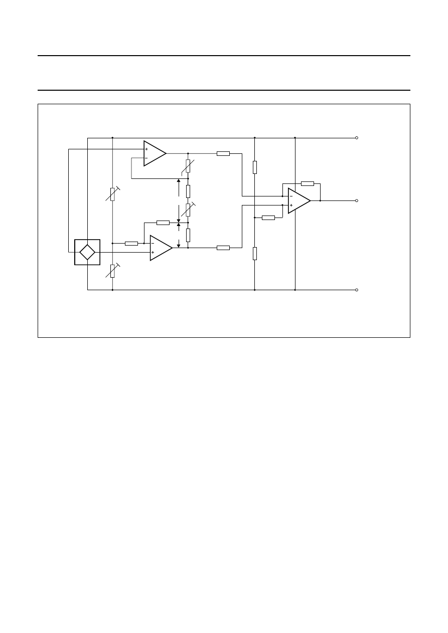
Figure 16 shows an example with a commonly-used
instrumentation amplifier. The circuit can be divided into
two stages: a differential amplifier stage that produces a
symmetrical output signal derived from the
magnetoresistive sensor, and an output stage that also
provides a reference to ground for the amplification stage.
To compensate for the negative sensor drift, as with the
above circuit the amplification is again given an equal but
positive temperature coefficient, by means of a
KTY81-110 silicon temperature sensor in the feedback
loop of the differential amplifier.
Fig.15 SOAR of a KMZ10B sensor as a function of
auxiliary field ‘H
x
’ and disturbing field ‘H
d
’
opposing ‘H
x
’ (area I).
handbook, halfpage
0
1
2
4
12
0
4
8
MLC133
3
Hd
(kA/m)
H (kA/m)
x
,,,,,,
,,,,,,
,,,,,,
,,,,,,
,,,,,,
,,,,,,
,,,,,,
I
II
SOAR
A
R
5
R
3
-------
=
1
2R
T
R
7
-----------
+
TC
A
TC
KTY
1
R
7
2R
T
-----------
+
---------------------
=
2000 Sep 06
14
Philips Semiconductors
Magnetoresistive sensors for
magnetic field measurement
General
Fig.16 KMZ10B application circuit with instrumentation amplifier.
handbook, full pagewidth
MLC145
KMZ10B
offset
R2
VO
VS
R1
R3
OP2
R7
R4
R6
R
KTY82-110
R5
R9
R10
R12
R11
R13
R14
OP1
OP3
T
RA
R B
The amplification of the input stage (‘OP1’ and ‘OP2’) is
given by:
(9)
where R
T
is the temperature dependent resistance of the
KTY82 sensor and R
B
is the bridge resistance of the
magnetoresistive sensor.
The amplification of the complete amplifier can be
calculated by:
(10)
The positive temperature coefficient (TC) of the
amplification is:
(11)
For the given negative ‘TC’ of the magnetoresistive sensor
and the required amplification of the input stage ‘A1’, the
resistance ‘R
A
’ and ‘R
B
’ can be calculated by:
(12)
(13)
where TC
KTY
is the temperature coefficient of the KTY
sensor and TC
A
is the temperature coefficient of the
amplifier. This circuit also provides for adjustment of gain
and offset voltage of the magnetic-field sensor.
A1
1
R
T
R
B
+
R
A
---------------------
+
=
A
A1
R
14
R
10
---------
×
=
TC
A
R
T
TC
KTY
×
R
A
R
B
R
T
+
+
-----------------------------------
=
R
B
R
T
TC
KTY
TC
A
------------------
1
1
A1
-------
–
1
–
×
×
=
R
A
R
T
R
B
+
A1
1
–
---------------------
=
2000 Sep 06
15
Philips Semiconductors
Magnetoresistive sensors for
magnetic field measurement
General
APPENDIX 1: THE MAGNETORESISTIVE EFFECT
Magnetoresistive sensors make use of the fact that the
electrical resistance
ρ
of certain ferromagnetic alloys is
influenced by external fields. This solid-state
magnetoresistive effect, or anisotropic magnetoresistance,
can be easily realized using thin film technology, so lends
itself to sensor applications.
Resistance
- field relation
The specific resistance
ρ
of anisotropic ferromagnetic
metals depends on the angle
Θ
between the internal
magnetization M and the current I, according to:
ρ(Θ) = ρ
⊥
+ (ρ
⊥
− ρ
||
)
cos
2
Θ
(1)
where
ρ
⊥
and
ρ
||
are the resistivities perpendicular and
parallel to M. The quotient
(ρ
⊥
− ρ
||
)/ρ
⊥
= ∆ρ/ρ
is called the magnetoresistive effect and may amount to
several percent.
Sensors are always made from ferromagnetic thin films as
this has two major advantages over bulk material: the
resistance is high and the anisotropy can be made
uniaxial. The ferromagnetic layer behaves like a single
domain and has one distinguished direction of
magnetization in its plane called the easy axis (e.a.),
which is the direction of magnetization without external
field influence.
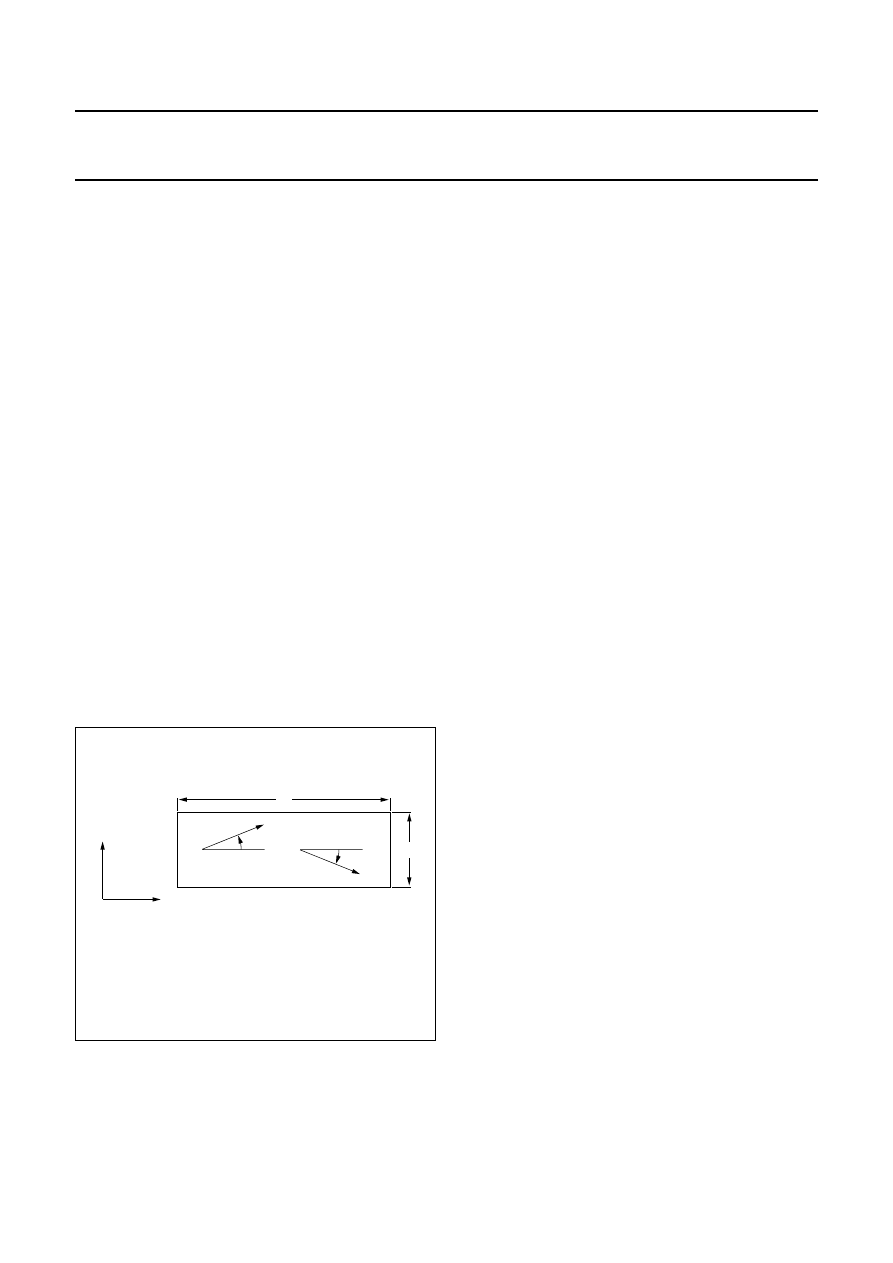
Figure 17 shows the geometry of a simple sensor where
the thickness (t) is much smaller than the width (w) which
is in turn, less than the length (l) (i.e. t « w ‹ l). With the
current (I) flowing in the x-direction (i.e. q = 0 or Q = f) then
the following equation can be obtained from equation 1:
R = R
0
+ DR cos
2
f(2)
and with a constant current
Ι
, the voltage drop in the
x-direction U
x
becomes:
U
x
=
ρ
⊥
Ι
(3)
Besides this voltage, which is directly allied to the
resistance variation, there is a voltage in the y-direction,
U
y
, given by:
U
y
= ρ
⊥
Ι
(4)
This is called the planar or pseudo Hall effect; it
resembles the normal or transverse Hall effect but has a
physically different origin.
All sensor signals are determined by the angle
φ
between
the magnetization M and the ‘length’ axis and, as M
rotates under the influence of external fields, these
external fields thus directly determine sensor signals. We
can assume that the sensor is manufactured such that the
e.a. is in the x-direction so that without the influence of
external fields, M only has an x-component
(
φ
= 0˚ or 180˚).
Two energies have to be introduced when M is rotated by
external magnetic fields: the anisotropy energy and the
demagnetizing energy. The anisotropy energy E
k
, is given
by the crystal anisotropy field H
k
, which depends on the
material and processes used in manufacture. The
demagnetizing energy E
d
or form anisotropy depends on
the geometry and this is generally a rather complex
relationship, apart from ellipsoids where a uniform
demagnetizing field H
d
may be introduced. In this case, for
the sensor set-up in Fig.17.
(5)
where the demagnetizing factor N
−
t/w, the saturation
magnetization M
s
≈
1 T and the induction constant
µ
0 = 4
π
-7
Vs/Am.
The field H
0
−
H
k
+ t/w(M
0
/m
0
) determines the measuring
range of a magnetoresistive sensor, as f is given by:
Fig.17 Geometry of a simple sensor.
handbook, halfpage
y
x
L
M
Ι
MBH616
ϕ
W
ϑ
L
wt
------
1
∆ρ
ρ
-------
cos
2
φ
+
1
t
---
∆ρ
ρ
-------
sin
φ
cos
φ
H
d
t
w
----
M
s
µ
0
-------
≈
2000 Sep 06
16
Philips Semiconductors
Magnetoresistive sensors for
magnetic field measurement
General
sin
φ =
(6)
where |H
y
|
≤
|H
0
+ H
x
| and H
x
and H
y
are the components
of the external field. In the simplest case H
x
= 0, the volt-
ages U
x
and U
y
become:
U
x
= ρ
⊥
l
(7)
U
y
= ρ
⊥
l
(8)
(Note: if H
x
= 0, then H
0
must be replaced by
H
0
+ H
x
/cos
φ
).
Neglecting the constant part in U
x
, there are two main
differences between U
x
and U
y
:
1. The magnetoresistive signal U
x
depends on the
square of H
y
/H
0
, whereas the Hall voltage U
y
is linear
for H
y
« H
0
.
2. The ratio of their maximum values is L/w; the Hall
voltage is much smaller as in most cases L » w.
Magnetization of the thin layer
The magnetic field is in reality slightly more complicated
than given in equation (6). There are two solutions for
angle
φ
:
φ
1 < 90˚ and
φ
2 > 90˚ (with
φ
1 +
φ
2 = 180˚ for H
x
= 0).
Replacing
φ
by 180˚ -
φ
has no influence on U
x
except to
change the sign of the Hall voltage and also that of most
linearized magnetoresistive sensors.
Therefore, to avoid ambiguity either a short pulse of a
proper field in the x-axis (|H
x
| > H
k
) with the correct sign
must be applied, which will switch the magnetization into
the desired state, or a stabilizing field Hst in the
x-direction can be used. With the exception of H
y
« H
0
, it
is advisable to use a stabilizing field as in this case, H
x
values are not affected by the non-ideal behaviour of the
layer or restricted by the so-called ‘blocking curve’.
The minimum value of H
st
depends on the structure of the
sensitive layer and has to be of the order of H
k
, as an
insufficient value will produce an open characteristic
(hysteresis) of the sensor. An easy axis in the y-direction
leads to a sensor of higher sensitivity, as then
H
o
= H
k
−
H
d
.
Linearization
As shown, the basic magnetoresistor has a square
resistance-field (R-H) dependence, so a simple
magnetoresistive element cannot be used directly for
linear field measurements. A magnetic biasing field can
be used to solve this problem, but a better solution is
linearization using barber-poles (described later).
Nevertheless plain elements are useful for applications
using strong magnetic fields which saturate the sensor,
where the actual value of the field is not being measured,
such as for angle measurement. In this case, the direction
of the magnetization is parallel to the field and the sensor
signal can be described by a cos
2
α
function.
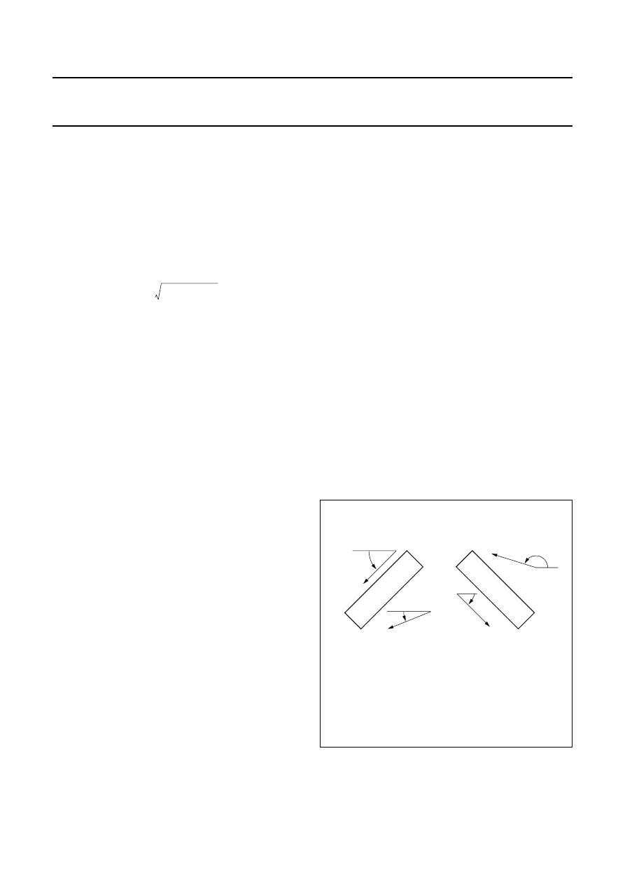
Sensors with inclined elements
Sensors can also be linearized by rotating the current path,
by using resistive elements inclined at an angle
θ
, as
shown in Fig.18. An actual device uses four inclined
resistive elements, two pairs each with opposite
inclinations, in a bridge.
The magnetic behaviour of such is pattern is more
complicated as M
o
is determined by the angle of inclination
θ
, anisotropy, demagnetization and bias field (if present).
Linearity is at its maximum for
φ
+
θ ≈
45˚, which can be
achieved through proper selection of
θ
.
A stabilization field (H
st
) in the x-direction may be
necessary for some applications, as this arrangement only
works properly in one magnetization state.
H
y
H
o
H
x
cos
φ
------------
+
--------------------------
L
wt
------
1
∆ρ
ρ
-------
1
H
y
H
0
-------
2
–
+
1
t
---
∆ρ
ρ
-------
H
y
H
0
-------
1
H
y
H
0
⁄
(
)
2
–
Fig.18 Current rotation by inclined elements
(current and magnetization shown in
quiescent state).
handbook, halfpage
MBH613
M0
M0
Ι
Ι
ϑ
ϑ
ϕ
ϕ
2000 Sep 06
17
Philips Semiconductors
Magnetoresistive sensors for
magnetic field measurement
General
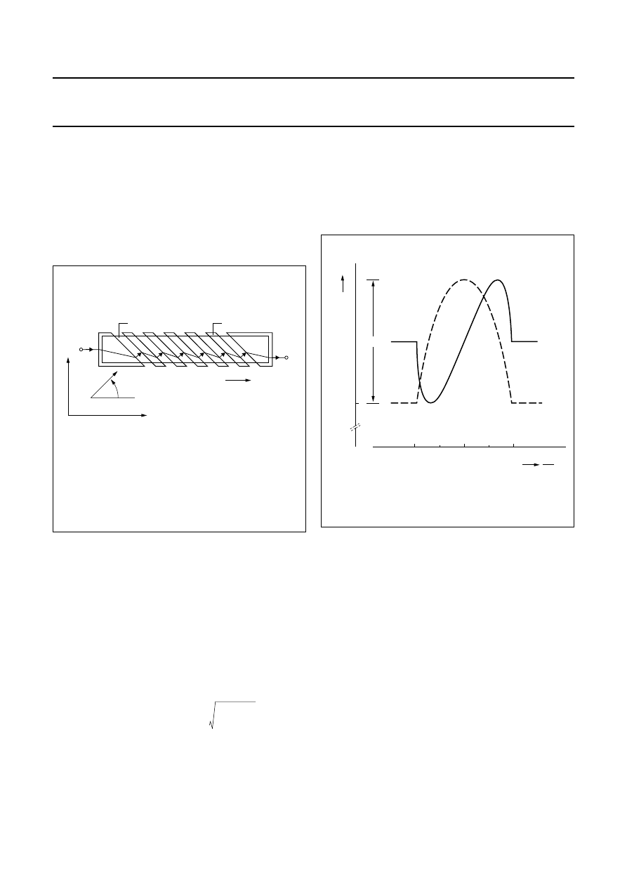
B
ARBER
-
POLE SENSORS
A number of Philips’ magnetoresistive sensors use a
‘barber-pole’ construction to linearize the R-H relationship,
incorporating slanted strips of a good conductor to rotate
the current. This type of sensor has the widest range of
linearity, smaller resistance and the least associated
distortion than any other form of linearization, and is well
suited to medium and high fields.
The current takes the shortest route in the high-resistivity
gaps which, as shown in Fig 19, is perpendicular to the
barber-poles. Barber-poles inclined in the opposite
direction will result in the opposite sign for the R-H
characteristic, making it extremely simple to realize a
Wheatstone bridge set-up.
The signal voltage of a Barber-pole sensor may be
calculated from the basic equation (1) with
Θ
=
φ
+ 45˚
(
θ
= + 45˚):
U
BP
= ρ
⊥
l
(9)
where a is a constant arising from the partial shorting of the
resistor, amounting to 0.25 if barber-poles and gaps have
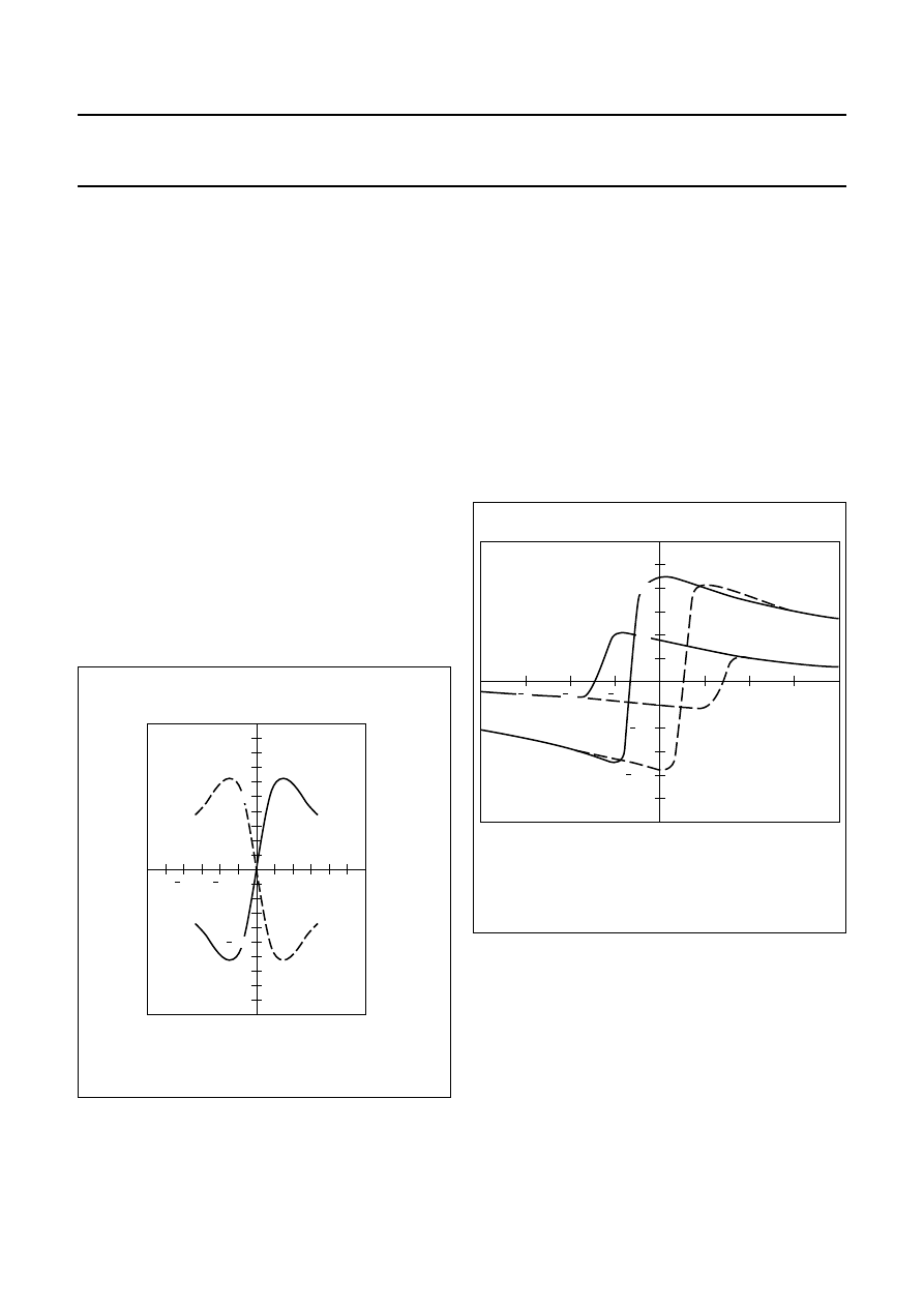
equal widths. The characteristic is plotted in Fig 20 and it
can be seen that for small values of H
y
relative to H
0
, the
R-H dependence is linear. In fact this equation gives the
same linear R-H dependence as the planar Hall-effect
sensor, but it has the magnitude of the magnetoresistive
sensor.
Barber-pole sensors require a certain magnetization
state. A bias field of several hundred A/m can be
generated by the sensing current alone, but this is not
sufficient for sensor stabilization, so can be neglected. In
most applications, an external field is applied for this
purpose.
Sensitivity
Due to the high demagnetization, in most applications
field components in the z-direction (perpendicular to the
layer plane) can be ignored. Nearly all sensors are most
sensitive to fields in the y-direction, with H
x
only having a
limited or even negligible influence.
Definition of the sensitivity S contains the signal and field
variations (DU and DH), as well as the operating voltage
U
0
(as D
U
is proportional to U
0
):
S
o
=
(10)
Fig.19 Linearization of the magnetoresistive effect
with barber-poles (current and
magnetization shown in quiescent state).
handbook, halfpage
Magnetization
Barber pole
Permalloy
Ι
Ι
y
+
Ι
−
x
ϑ
,,,,
,,,,
,,,,
,,,
,,,
,,,
,,,
,,,
,,,
,,,
,,,
,,,
,,
,,
,,
,,,
,,,
,,,
,,,
,,,
,,,
MBH614
L
wt
------
α
1
1
2
---
∆ρ
ρ
-------
∆ρ
ρ
-------
±
H
y
H
0
------- 1
H
y
H
0
-------
2
–
+
Fig.20 Calculated R-H characteristic of a
barber-pole sensor.
handbook, halfpage
MBH615
−
0.5
0
0
R0
R
∆
R
0.5
1
HY
H0
−
1
∆
U
∆
H
--------
1
U
0
-------
∆
U
U
0
∆
H
----------------
=

2000 Sep 06
18
Philips Semiconductors
Magnetoresistive sensors for
magnetic field measurement
General
This definition relates DU to a unit operating voltage.
The highest (H
G
) and lowest (H
min
) fields detectable by
the sensor are also of significance. The measuring range
H
G
is restricted by non-linearity - if this is assumed at 5%,
an approximate value for barber-pole sensors is given by:
(11)
From this and equation (9) for signal voltage (U
BP
) for a
barber-pole sensor, the following simple relationship can
be obtained:
(12)
Other sensor types have a narrower range of linearity and
therefore a smaller useful signal.
The lowest detectable field H
min
is limited by offset, drift
and noise. The offset is nearly cancelled in a bridge circuit
and the remaining imbalance is minimized by symmetrical
design and offset trimming, with thermal noise negligible in
most applications (see section on sensor layout). Proper
film deposition and, if necessary, the introduction of a
stabilization field will eliminate magnetization switching
due to domain splitting and the introduction of ‘Barkhausen
noise’.
Sensitivity S
0
is essentially determined by the sum of the
anisotropy (H
k
), demagnetization (H
d
) and bias (H
x
) fields.
The highest sensitivity is achievable with H
x
= 0 and
H
d
« H
k
, although in this case S
0
depends purely on H
k
which is less stable than H
d
. For a permalloy with a
thickness greater than or equal to 20
µ
m, a width in
excess of 60
µ
m is required which, although possible, has
the drawback of producing a very low resistance per unit
area.
The maximum theoretical S
0
with this permalloy (at
H
k
= 250 A/m and
∆ρ/ρ
= 2.5%) is approximately:
(13)
For the same reasons, sensors with reduced sensitivity
should be realized with increased H
d
, which can be esti-
mated at a maximum for a barber-pole sensor at 40 kA/m.
A further reduction in sensitivity and a corresponding
growth in the linearity range is attained using a biasing
field. A magnetic shunt parallel to the magnetoresistor or
only having a small field component in the sensitive direc-
tion can also be employed with very high field strengths.
A high signal voltage U
x
can only be produced with a
sensor that can tolerate a high supply voltage U
o
. This
requires a high sensor resistance R with a large area A,
since there are limits for power dissipation and current
density. The current density in permalloy may be very high
(j > 10
6
A/cm
2
in passivation layers), but there are weak
points at the current reversal in the meander (see section
on sensor layout) and in the barber-pole material, with
five-fold increased current density.
A high resistance sensor with U
0
= 25 V and a maximum
S
0
results in a value of 2.5 x 10
-3
(A/m)
-1
for Su or, converted to flux density, S
T
= 2000 V/T.
This value is several orders of magnitude higher than for a
normal Hall effect sensor, but is valid only for a much
narrower measuring range.
Materials
There are five major criteria for a magnetoresistive
material:
•
Large magnetoresistive effect Dr/r (resulting in a high
signal to operating voltage ratio)
•
Large specific resistance r (to achieve high resistance
value over a small area)
•
Low anisotropy
•
Zero magnetostriction (to avoid influence of mechanical
stress)
•
Long-term stability.
Appropriate materials are binary and ternary alloys of Ni,
Fe and Co, of which NiFe (81/19) is probably the most
common.
Table 1 gives a comparison between some of the more
common materials, although the majority of the figures are
only approximations as the exact values depend on a
number of variables such as thickness, deposition and
post-processing.
Table 3
Comparison of magnetoresistive sensor
materials
∆ρ
is nearly independent of these factors, but r itself
increases with thickness (t
≤
40 nm) and will decrease
during annealing. Permalloys have a low H
k
and zero
magnetostriction; the addition of C
o
will increase
∆ρ/ρ
, but
H
G
0.5 H
0
H
x
+
(
)
≈
H
G
S
0
0.5
∆ρ
ρ
-------
≈
S
0
(max)
10
4
–
A
m
-----
1
100
mV
V
---------
kA
m
-------
--------------
=
=
Materials
ρ
(10
−
8
Ω
m)
∆ρ
/
ρ
(%)
ΙΙ
k
(
∆
/m)
NiFe 81:19
22
2.2
250
NiFe 86:14
15
3
200
NiCo 50:50
24
2.2
2500
NiCo 70:30
26
3.7
2500
CoFeB 72:8:20
86
0.07
2000
2000 Sep 06
19
Philips Semiconductors
Magnetoresistive sensors for
magnetic field measurement
General
this also considerably enlarges H
k
. If a small temperature
coefficient of
∆ρ
is required, NiCo alloys are preferable.
The amorphous alloy CoFeB has a low
∆ρ/ρ
, high H
k
and
slightly worse thermal stability but due to the absence of
grain boundaries within the amorphous structure, exhibits
excellent magnetic behaviour.
APPENDIX 2: SENSOR FLIPPING
During deposition of the permalloy strip, a strong external
magnetic field is applied parallel to the strip axis. This
accentuates the inherent magnetic anisotropy of the strip
and gives them a preferred magnetization direction, so that
even in the absence of an external magnetic field, the
magnetization will always tend to align with the strips.
Providing a high level of premagnetization within the
crystal structure of the permalloy allows for two stable
premagnetization directions. When the sensor is placed in
a controlled external magnetic field opposing the internal
aligning field, the polarity of the premagnetization of the
strips can be switched or ‘flipped’ between positive and
negative magnetization directions, resulting in two stable
output characteristics.
The field required to flip the sensor magnetization (and
hence the output characteristic) depends on the
magnitude of the transverse field H
y
. The greater this field,
the more the magnetization rotates towards 90˚ and
therefore it becomes easier to flip the sensor into the
corresponding stable position in the ‘-x’ direction. This
means that a smaller -H
x
field is sufficient to cause the
flipping action
As can be seen in Fig 22, for low transverse field strengths
(0.5 kA/m) the sensor characteristic is stable for all positive
values of H
x
, and a reverse field of approximately 1 kA/m
is required to flip the sensor. However at higher values of
H
y
(2 kA/m), the sensor will also flip for smaller values of
H
x
(at 0.5 kA/m). Also illustrated in this figure is a
noticeable hysteresis effect; it also shows that as the
permalloy strips do not flip at the same rate, the flipping
action is not instantaneous.
The sensitivity of the sensor reduces as the auxiliary field
H
x
increases, which can be seen in Fig 22 and more
clearly in Fig 23. This is because the moment imposed on
the magnetization by H
x
directly opposes that of H
y
,
resulting in a reduction in the degree of bridge imbalance
and hence the output signal for a given value of H
y
.
Fig.21 Sensor characteristics.
handbook, halfpage
MLC130
0
2
4
2
4
O
(mV)
H (kA/m)
y
V
10
10
reversal
of sensor
characteristics
Fig.22 Sensor output ‘V
o
’ as a function of the
auxiliary field H
x
.
MLC131
0
1
2
3
1
O
(mV)
H (kA/m)
x
H =
2 kA/m
y
0.5 kA/m
V
50
100
100
50
2
3
2000 Sep 06
20
Philips Semiconductors
Magnetoresistive sensors for
magnetic field measurement
General
Fig.23 Sensor output ‘V
o
’ as a function of the transverse field H
y
.
handbook, full pagewidth
MLC132
0
2
4
6
8
10
12
O
(mV)
H (kA/m)
y
H =
4 kA/m
x
2 kA/m
1 kA/m
0
V
100
150
50
A Safe Operating ARea (SOAR) can be determined for
magnetoresistive sensors, within which the sensor will not
flip, depending on a number of factors. The higher the
auxiliary field, the more tolerant the sensor becomes to
external disturbing fields (H
d
) and with an H
x
of 3 kA/m or
greater, the sensor is stabilized for all disturbing fields as
long as it does not irreversibly demagnetize the sensor. If
Hd is negative and much larger than the stabilising field H
x
,
the sensor will flip. This effect is reversible, with the sensor
returning to the normal operating mode if H
d
again
becomes negligible (see Fig 24). However the higher H
x
,
the greater the reduction in sensor sensitivity and so it is
generally recommended to have a minimum auxiliary field
that ensures stable operation, generally around 1 kA/m.
The SOAR can also be extended for low values of H
x
as
long as the transverse field is less than 1 kA/m. It is also
recommended to apply a large positive auxiliary field
before first using the sensor, which erases any residual
hysteresis
Fig.24 SOAR of a KMZ10B sensor as a function of
auxiliary field ‘H
x
’ (MLC133).
handbook, halfpage
0
1
2
4
12
0
4
8
MLC133
3
Hd
(kA/m)
H (kA/m)
x
,,,,,,
,,,,,,
,,,,,,
,,,,,,
,,,,,,
,,,,,,
,,,,,,
I
II
SOAR
2000 Sep 06
21
Philips Semiconductors
Magnetoresistive sensors for
magnetic field measurement
General
APPENDIX 3: SENSOR LAYOUT
In Philips’ magnetoresistive sensors, the permalloy strips
are formed into a meander pattern on the silicon substrate.
With the KMZ10 (see Fig 25) and KMZ51 series, four
barber-pole permalloy strips are used while the KMZ41
series has simple elements. The patterns used are
different for these three families of sensors in every case,
the elements are linked in the same fashion to form the four
arms of a Wheatstone bridge. The meander pattern used
in the KMZ51 is more sophisticated and also includes
integrated compensation and flipping coils (see chapter on
weak fields); the KMZ41 is described in more detail in the
chapter on angle measurement.
Fig.25 KMZ10 chip structure.
handbook, full pagewidth
MBC930
,,,,,
,,,,,
,,,,,
,,,,,
,,,,,
,,,,,
,,,,,
,,,,,
,,,,,
,,,,,
,,,,,
,,,,,
,,,,,
,,,,,
,,,,,
,,,,,
,,,,,
,,,,,
,,,,,
,,,,,
,,,,,
,,,,,
,,,,,
,,,,,
,,,,,
,,,,,,
,,,,,,
,,,,,,
,,,,,,
,,,,,,
,,,,,,
,,,,,,
,,,,,,
,,,,,,
,,,,,,
,,,,,,
,,,,,,
,,,,,
,,,,,,
,,,,,,
,,,,,,
,,,,,,
,,,,,,
,,,,,,
,,,,,,
,,,,,,
,,,,,,
,,,,,,
,,,,,,
,,,,,,
,,,,,,
,,,,,,
2000 Sep 06
22
Philips Semiconductors
Magnetoresistive sensors for
magnetic field measurement
General
In one pair of diagonally opposed elements the
barber-poles are at +45˚ to the strip axis, with the second
pair at
−
45˚. A resistance increase in one pair of elements
due to an external magnetic field is matched by an equal
decrease in resistance of the second pair. The resulting
bridge imbalance is then a linear function of the amplitude
of the external magnetic field in the plane of the permalloy
strips normal to the strip axis.
This layout largely eliminates the effects of ambient
variations (e.g. temperature) on the individual elements
and also magnifies the degree of bridge imbalance,
increasing sensitivity.
Fig 26 indicates two further trimming resistors (R
T
) which
allow the sensors electrical offset to be trimmed down to
zero during the production process.
Fig.26 KMZ10 and KMZ11 bridge configuration.
handbook, halfpage
MLC129
2
1
GND
VO
VCC
VO
RT
RT
3
4
2000 Sep 06
23
Philips Semiconductors
Magnetoresistive sensors for
magnetic field measurement
General
WEAK FIELD MEASUREMENT
Contents
•
Fundamental measurement techniques
•
Application note AN00022: Electronic compass design
using KMZ51 and KMZ52
•
Application circuit: signal conditioning unit for compass
•
Example 1: Earth geomagnetic field compensation in
CRT’s
•
Example 2: Traffic detection
•
Example 3: Measurement of current.
Fundamental measurement techniques
Measurement of weak magnetic fields such as the earth’s
geomagnetic field (which has a typical strength of between
approximately 30 A/m and 50 A/m), or fields resulting from
very small currents, requires a sensor with very high
sensitivity. With their inherent high sensitivity,
magnetoresistive sensors are extremely well suited to
sensing very small fields.
Philips’ magnetoresistive sensors are by nature bi-stable
(refer to Appendix 2). ‘Standard’ techniques used to
stabilize such sensors, including the application of a strong
field in the x-direction (H
x
) from a permanent stabilization
magnet, are unsuitable as they reduce the sensor’s
sensitivity to fields in the measurement, or y-direction (H
y
).
(Refer to Appendix 2, Fig. A2.2).
To avoid this loss in sensitivity, magnetoresistive sensors
can instead be stabilized by applying brief, strong
non-permanent field pulses of very short duration (a few
µ
s). This magnetic field, which can be easily generated by
simply winding a coil around the sensor, has the same
stabilizing effect as a permanent magnet, but as it is only
present for a very short duration, after the pulse there is no
loss of sensitivity. Modern magnetoresistive sensors
specifically designed for weak field applications
incorporate this coil on the silicon.
However, when measuring weak fields, second order
effects such as sensor offset and temperature effects can
greatly reduce both the sensitivity and accuracy of MR
sensors. Compensation techniques are required to
suppress these effects.
O
FFSET COMPENSATION BY
‘
FLIPPING
’
Despite electrical trimming, MR sensors may have a
maximum offset voltage of
±
1.5 mV/V. In addition to this
static offset, an offset drift due to temperature variations of
about 6 (
µ
V/V)K
−
1
can be expected and assuming an
ambient temperature up to 100
°
C, the resulting offset can
be of the order of 2 mV/V.
Taking these factors into account, with no external field a
sensor with a typical sensitivity of 15 mV/V (kA/m)
−
1
can
have an offset equivalent to a field of 130 A/m, which is
itself about four times the strength of a typical weak field
such as the earth’s geomagnetic field. Clearly, measures
to compensate for the sensor offset value have to be
implemented in weak field applications.
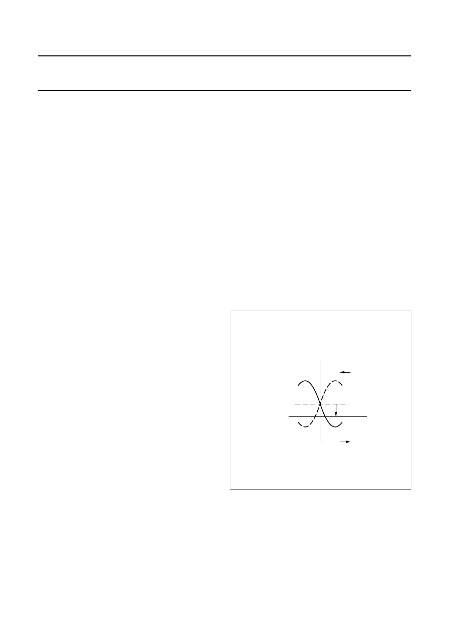
A technique called ‘flipping’ (patented by Philips) can be
used to control the sensor. Comparable to the ‘chopping’
technique used in the amplification of small electrical
signals, it not only stabilizes the sensor but also eliminates
the described offset effects.
When the bi-stable sensor is placed in a controlled,
reversible external magnetic field, the polarity of the
premagnetization (M
x
) of the sensor strips can be switched
or flipped between the two output characteristics (see
Fig.27).
This reversible external magnetic field can be easily
achieved with a coil wound around the sensor, consisting
of current carrying wires, as described above. Depending
on the direction of current pulses through this coil, positive
and negative flipping fields in the x-direction (+H
x
and
−
H
x
)
are generated (see Fig.28).
Fig.27 Butterfly curve including offset.
MLC764
VO
M x
offset
H y
M x
2000 Sep 06
24
Philips Semiconductors
Magnetoresistive sensors for
magnetic field measurement
General
Flipping causes a change in the polarity of the sensor
output signal and this can be used to separate the offset
signal from the measured signal. Essentially, the unknown
field in the ‘normal’ positive direction (plus the offset) is
measured in one half of the cycle, while the unknown field
in the ‘inverted’ negative direction (plus the offset) is
measured in the second half. This results in two different
outputs symmetrically positioned around the offset value.
After high pass filtering and rectification a single,
continuous value free of offset is output, smoothed by low
pass filtering. See Figs 29 and 30.
Offset compensation using flipping requires additional
external circuitry to recover the measured signal.
Fig.28 Flipping coil.
MLC762
H y
Hx
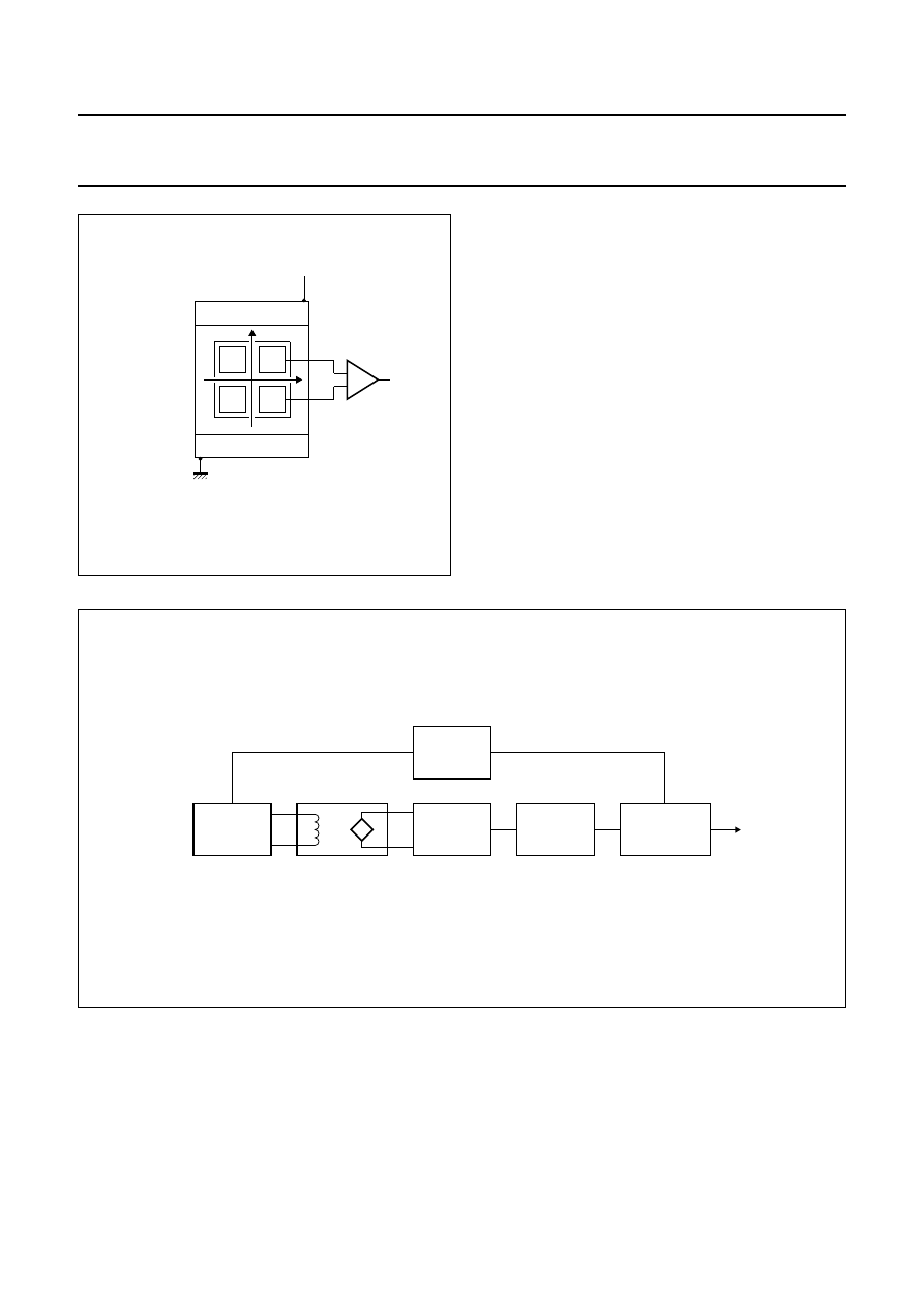
coil
,,,,
,,,,
,,,,
,
,
,
,
,
,
,
,
VO
current
pulses
sensor
Fig.29 Block diagram of flipping circuit.
handbook, full pagewidth
MBH617
LF
IF
FLIPPING
SOURCE
PRE-
AMPLIFIER
CLOCK
T
OFFSET
FILTER
Vout
PHASE
SENSITIVE
DEMODULATOR
2000 Sep 06
25
Philips Semiconductors
Magnetoresistive sensors for
magnetic field measurement
General
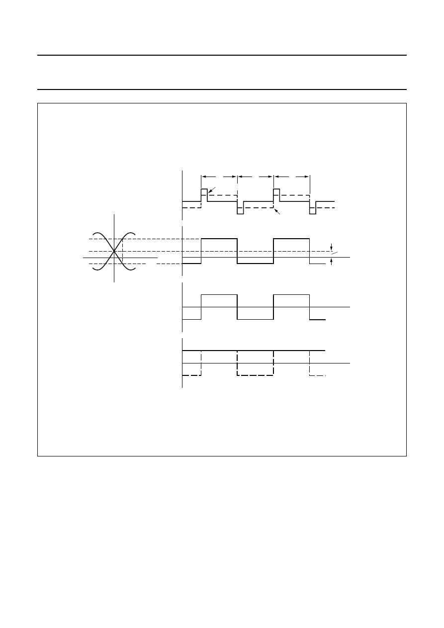
Fig.30 Timing diagram for flipping circuit (a) output voltage; (b) filtered output voltage; (c) output voltage filtered
and demodulated.
handbook, full pagewidth
MBH618
offset
internal
magnetization
flipping current IF
VO
T
time
time
VO
time
VO
time
VO
Hy
T
T
(a)
(b)
(c)
2000 Sep 06
26
Philips Semiconductors
Magnetoresistive sensors for
magnetic field measurement
General
S
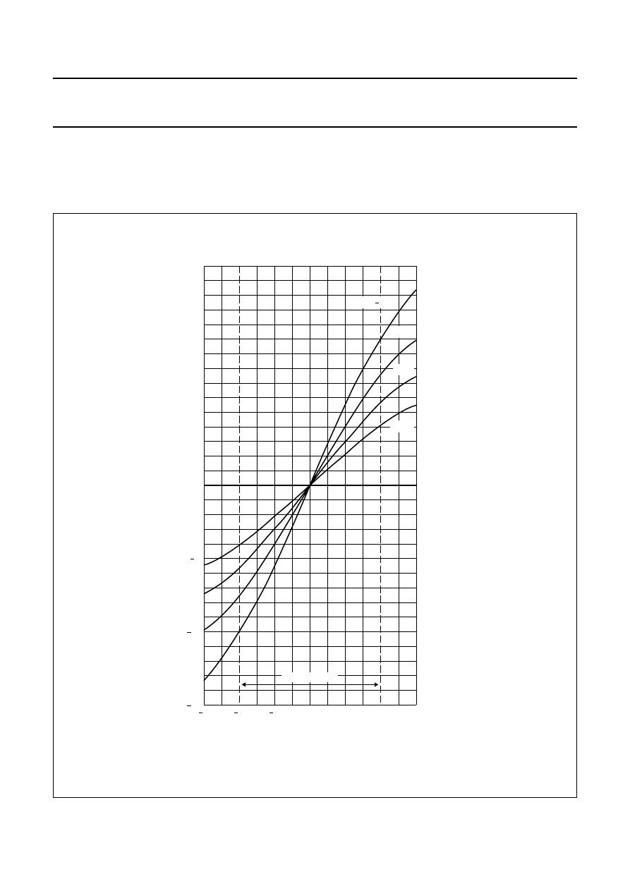
ENSOR TEMPERATURE DRIFT
The sensitivity of MR sensors is also temperature
dependent, with sensitivity decreasing as temperature
increases (Fig.31).The effect on sensor output is certainly
not negligible, as it can produce a difference of a factor of
three within a
−
25
°
C to +125
°
C temperature range, for
fields up to 0.5 kA/m. This effect is not compensated for by
the flipping action described in the last section.
Fig.31 Output voltage ‘V
o
’ as a fraction of the supply voltage for a KMZ10B sensor, as a function of transverse
field ‘H
y
’, at several temperatures.
handbook, full pagewidth
3
0
15
3
2
2
MLC134
5
10
10
5
15
0
1
1
H (kA/m)
y
VO
(mV/V)
T = 25 C
amb
o
25 C
o
75 C
o
125 C
o
operating range
2000 Sep 06
27
Philips Semiconductors
Magnetoresistive sensors for
magnetic field measurement
General
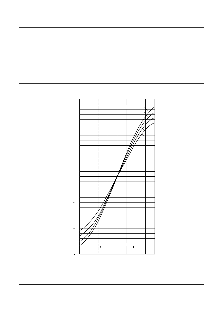
The simplest form of temperature compensation is to use
a current source to supply to the sensor instead of a
voltage source. In this case, the resulting reduction in
sensitivity due to temperature is partially compensated by
a corresponding increase in bridge resistance.
Thus a current source not only improves the stability of the
output voltage ‘V
o
’, and reduces the variation in sensitivity
to a factor of approximately 1.5 (compared to a factor of
three using the voltage source). However, this method
requires a higher supply voltage, due to the voltage drop
of the current source.
Fig.32 Output voltage ‘V
o
’ of a KMZ10B sensor as a function of transverse field ‘H
y
’ using a current source, for
several temperatures.
handbook, full pagewidth
0
75
4
2
MLC135
25
50
50
25
75
2
0
4
H (kA/m)
y
VO
(mV/V)
T = 25 C
amb
o
25 C
o
75 C
o
125 C
o
operating range
2000 Sep 06
28
Philips Semiconductors
Magnetoresistive sensors for
magnetic field measurement
General
The optimal method of compensating for temperature
dependent sensitivity differences in MR measurements of
weak fields uses electro-magnetic feedback. As can be
seen from the sensor characteristics in Figs 31 and 32,
sensor output is completely independent of temperature
changes at the point where no external field is applied
(the null-point). By using an electro-magnetic feedback
set-up, it is possible to ensure the sensor is always
operated at this point.
To achieve this, a second compensation coil is wrapped
around the sensor perpendicular to the flipping coil, so that
the magnetic field produced by this coil is in the same
plane as the field being measured.
Should the measured magnetic field vary, the sensor’s
output voltage will change, but the change will be different
at different ambient temperatures. This voltage change is
converted into a current by an integral controller and
supplied to the compensation coil, which then itself
produces a magnetic field proportional to the output
voltage change caused by the change in measured field.
The magnetic field produced by the compensation coil is in
the opposite direction to the measured field, so when it is
added to the measured field, it compensates exactly for
the change in the output signal, regardless of its actual,
temperature-dependent value. This principle is called
current compensation and because the sensor is always
used at its ‘zero’ point, compensation current is
independent of the actual sensitivity of the sensor or
sensitivity drift with temperature.
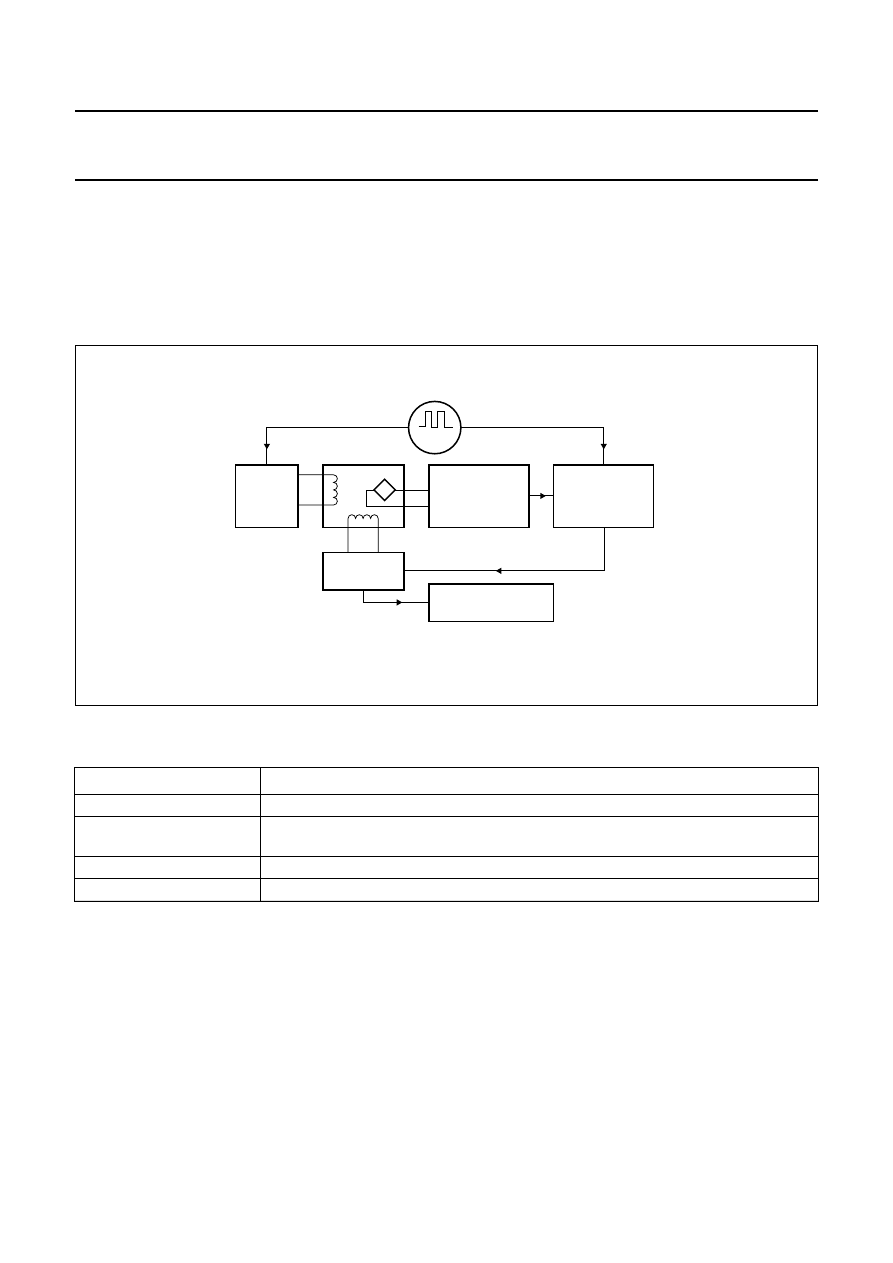
Information on the measured magnetic signal is effectively
given by the current fed to the compensating coil. If the
field factor of the compensation coil is known, this
simplifies calculation of the compensating field from the
compensating current and therefore the calculation of the
measured magnetic field. If this field factor is not precisely
known, then the resistor performing the current/voltage
conversion must be trimmed. Figure 34 shows a block
diagram of a compensated sensor set-up including the
flipping circuit.
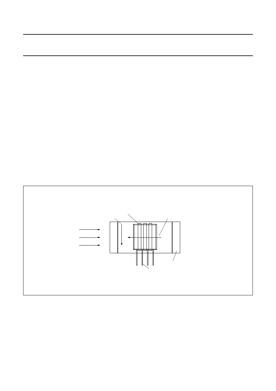
Fig.33 Magnetic field directions and the flipping and compensation coils.
handbook, full pagewidth
,,
,,
,,
,,
,,
,,
,,
,,
,
,
,
,
,
,
,,
,,
,,
flipping coil
sensor KMZ10A1
compensation coil
compensation field
flipping field
earth's field
MLC757
2000 Sep 06
29
Philips Semiconductors
Magnetoresistive sensors for
magnetic field measurement
General
The influence of other disturbing fields can also be
eliminated provided they are well known, by adding a
second current source to the compensating coil. Such
fields might be those arising from the set-up housing,
ferromagnetic components placed close to the sensor or
magnetic fields from electrical motors.
The brief summary in Table 3 compares the types of
compensation and their effects, so they can be assessed
for their suitability in a given application. Because these
options encompass a range of costs, the individual
requirements of an application should be carefully
analysed in terms of the performance gains versus relative
costs.
Table 4
Summery of compensation techniques
TECHNIQUE
EFFECT
Setting
avoids reduction in sensitivity due to constant stabilization field
Flipping
avoids reduction in sensitivity due to constant stabilization field, as well as
compensating for sensor offset and offset drift due to temperature
Current supply
reduction of sensitivity drift with temperature by a factor of two
Electro-magnetic feedback
accurate compensation of sensitivity drift with temperature
Fig.34 Block diagram of compensation circuit.
handbook, full pagewidth
MBH619
LF
LC
CURRENT
REGULATOR
FLIPPING
SOURCE
CLOCK
VOLTAGE & CURRENT
OUTPUT
PRE-AMPLIFIER
WITH
SUPRESSION
OF OFFSET
PHASE-
SENSITIVE
DEMODULATOR
2000 Sep 06
30
Philips Semiconductors
Magnetoresistive sensors for
magnetic field measurement
General
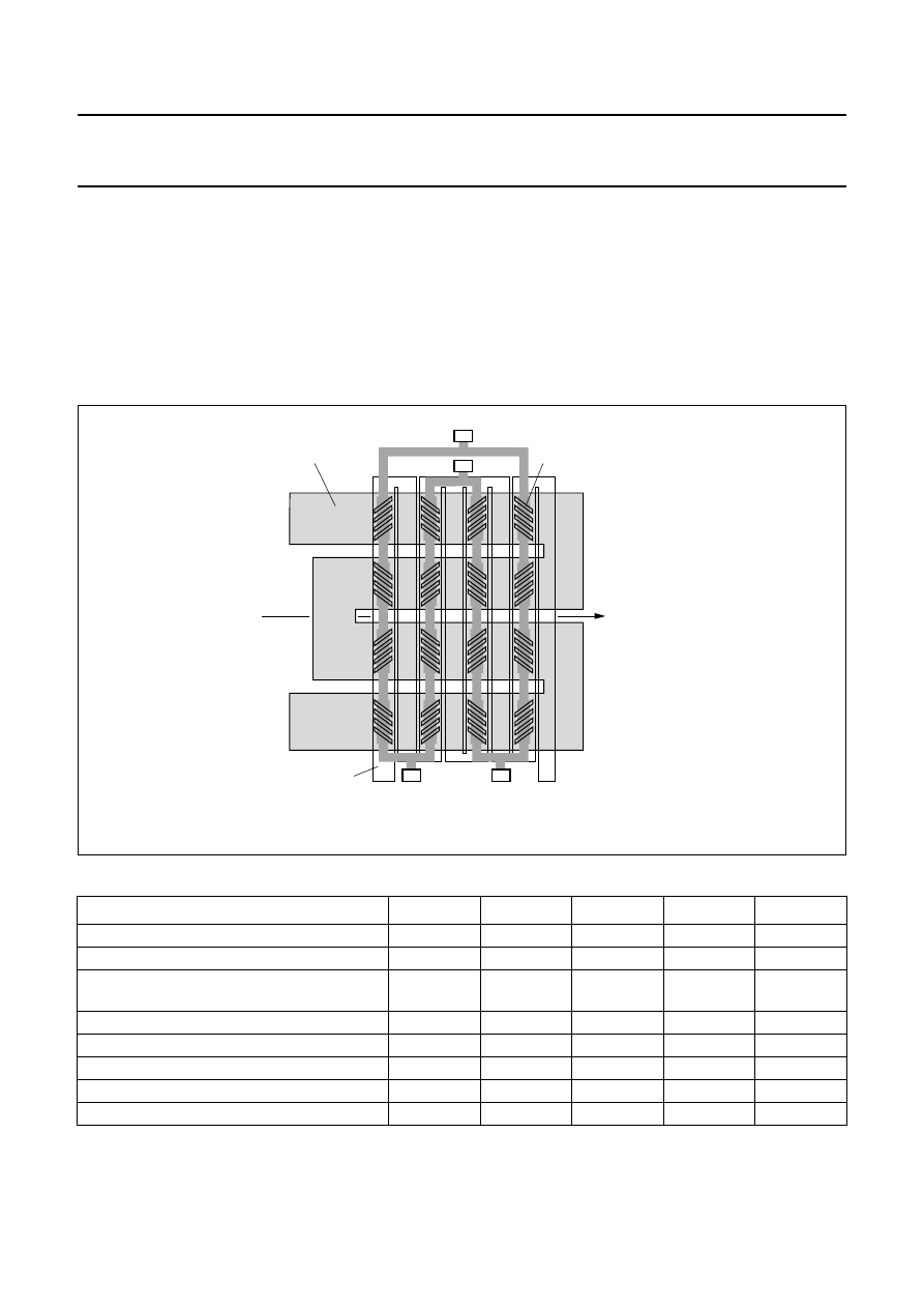
P
HILIPS SENSORS FOR WEAK FIELD MEASUREMENT
Philips Semiconductors has at present four different
sensors suitable for weak field applications, with the
primary device being the KMZ51, an extremely sensitive
sensor with integrated compensation and set/reset
coils.(see Fig.35)
This sensor is ideal for many weak field detection
applications such as compasses, navigation, current
measurement, earth magnetic field compensation, traffic
detection and so on. The integrated set/reset coils provide
for both the flipping required in weak field sensors and also
allow setting/resetting the orientation of the sensitivity after
proximity to large disturbing magnetic fields. Philips also
has the KMZ10A and KMZ10A1, similar sensors which do
not have integrated coils and therefore require external
coils. Table 5 provides a summary of the main single
sensors in Philips’ portfolio for weak field measurement.
Table 5
Properties of Philips Semiconductors single sensors for a weak field applications
Note
1. H
x
= 0.5 kA/m.
KMZ10A
KMZ10A1
KMZ51
KMZ52
UNIT
Package
SOT195
SOT195
SO8
SO16
−
Supply voltage
5
5
5
5
V
Sensitivity
16
(1)
22
16
16
(mV/V)/
(kA/m)
Offset voltage
±
1.5
±
1.5
±
1
±
1.5
mV/V
Offset voltage temperature drift
±
6
±
6
±
3
±
3
µ
V/V/K
Applicable field range (y-direction)
±
0.5
±
0.5
±
0.2
±
0.2
kA/m
Set/reset coil on-board
no
no
yes
yes
−
Compensation coil on-board
no
no
yes
yes
−
Fig.35 Layout of Philips’ KMZ51 magnetoresistive sensor.
handbook, full pagewidth
MBH630
barber-pole
flip conductor
compensation
conductor
Hy
(field to be
measured)

2000 Sep 06
31
Philips Semiconductors
Magnetoresistive sensors for
magnetic field measurement
General

2000 Sep 06
32
Philips Semiconductors
Magnetoresistive sensors for
magnetic field measurement
General

2000 Sep 06
33
Philips Semiconductors
Magnetoresistive sensors for
magnetic field measurement
General

2000 Sep 06
34
Philips Semiconductors
Magnetoresistive sensors for
magnetic field measurement
General

2000 Sep 06
35
Philips Semiconductors
Magnetoresistive sensors for
magnetic field measurement
General

2000 Sep 06
36
Philips Semiconductors
Magnetoresistive sensors for
magnetic field measurement
General

2000 Sep 06
37
Philips Semiconductors
Magnetoresistive sensors for
magnetic field measurement
General

2000 Sep 06
38
Philips Semiconductors
Magnetoresistive sensors for
magnetic field measurement
General

2000 Sep 06
39
Philips Semiconductors
Magnetoresistive sensors for
magnetic field measurement
General

2000 Sep 06
40
Philips Semiconductors
Magnetoresistive sensors for
magnetic field measurement
General

2000 Sep 06
41
Philips Semiconductors
Magnetoresistive sensors for
magnetic field measurement
General

2000 Sep 06
42
Philips Semiconductors
Magnetoresistive sensors for
magnetic field measurement
General

2000 Sep 06
43
Philips Semiconductors
Magnetoresistive sensors for
magnetic field measurement
General

2000 Sep 06
44
Philips Semiconductors
Magnetoresistive sensors for
magnetic field measurement
General

2000 Sep 06
45
Philips Semiconductors
Magnetoresistive sensors for
magnetic field measurement
General

2000 Sep 06
46
Philips Semiconductors
Magnetoresistive sensors for
magnetic field measurement
General

2000 Sep 06
47
Philips Semiconductors
Magnetoresistive sensors for
magnetic field measurement
General

2000 Sep 06
48
Philips Semiconductors
Magnetoresistive sensors for
magnetic field measurement
General

2000 Sep 06
49
Philips Semiconductors
Magnetoresistive sensors for
magnetic field measurement
General

2000 Sep 06
50
Philips Semiconductors
Magnetoresistive sensors for
magnetic field measurement
General

2000 Sep 06
51
Philips Semiconductors
Magnetoresistive sensors for
magnetic field measurement
General

2000 Sep 06
52
Philips Semiconductors
Magnetoresistive sensors for
magnetic field measurement
General

2000 Sep 06
53
Philips Semiconductors
Magnetoresistive sensors for
magnetic field measurement
General

2000 Sep 06
54
Philips Semiconductors
Magnetoresistive sensors for
magnetic field measurement
General

2000 Sep 06
55
Philips Semiconductors
Magnetoresistive sensors for
magnetic field measurement
General

2000 Sep 06
56
Philips Semiconductors
Magnetoresistive sensors for
magnetic field measurement
General

2000 Sep 06
57
Philips Semiconductors
Magnetoresistive sensors for
magnetic field measurement
General

2000 Sep 06
58
Philips Semiconductors
Magnetoresistive sensors for
magnetic field measurement
General

2000 Sep 06
59
Philips Semiconductors
Magnetoresistive sensors for
magnetic field measurement
General

2000 Sep 06
60
Philips Semiconductors
Magnetoresistive sensors for
magnetic field measurement
General

2000 Sep 06
61
Philips Semiconductors
Magnetoresistive sensors for
magnetic field measurement
General

2000 Sep 06
62
Philips Semiconductors
Magnetoresistive sensors for
magnetic field measurement
General

2000 Sep 06
63
Philips Semiconductors
Magnetoresistive sensors for
magnetic field measurement
General

2000 Sep 06
64
Philips Semiconductors
Magnetoresistive sensors for
magnetic field measurement
General

2000 Sep 06
65
Philips Semiconductors
Magnetoresistive sensors for
magnetic field measurement
General

2000 Sep 06
66
Philips Semiconductors
Magnetoresistive sensors for
magnetic field measurement
General
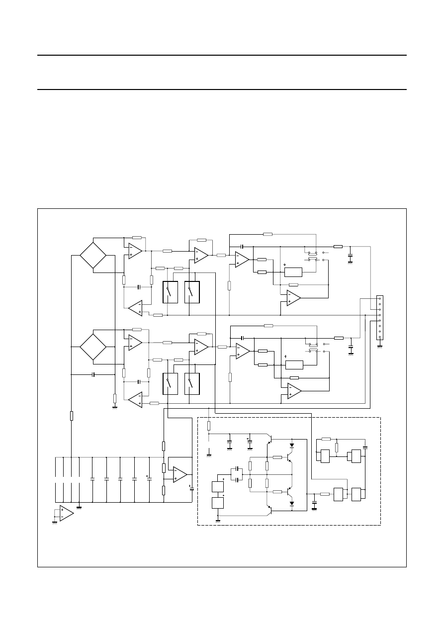
2000 Sep 06
67
Philips Semiconductors
Magnetoresistive sensors for
magnetic field measurement
General
APPLICATION CIRCUIT
Signal conditioning unit for compass
Fig.36 shows a dimensioned circuit that provides the
signal conditioning for both outputs of a KMZ52 (or two
KMZ51), as required in a compass application.
The circuit delivers the output voltages Vx and Vy, which
are proportional to the magnetic field measured in the x
and y directions respectively.
The operational principal of the circuit is based on that
described in section 5.
The circuit has the following characteristics:
•
supply voltage 10 V
•
flip frequency
≈
500 Hz
•
sensitivity
≈
30 mV per A/m
•
bandwidth
≈
10 Hz.
For demonstration purposes, the circuit can be operated
with or without electromagnetic feedback, depending on
the state of switches S1 and S2.
handbook, full pagewidth
MLD428
IC1C
IC1D
R4
100 k
Ω
R8
5.6 k
Ω
R14
5.6 k
Ω
R6
100
k
Ω
R5
100
k
Ω
C2
470 nF
R10
100 k
Ω
IC2D
IC2C
R15
10 k
Ω
R16
10 k
Ω
R19
20 k
Ω
R43
22
Ω
IC6D
CLOCK
CLOCK
CLK
CLK
IC6B
IC6C
HEF
4011BT
HEF
4011BT
HEF
4011BT
IC3C
IC3D
IC6A
HEF
4011BT
IC4D
IC4C
R20
20 k
Ω
R29
390
Ω
Vy
REF
Vx
+10 V
GND
C4
220 nF
KMZ52
R30
390
Ω
D2
BAS32L
BAS32L
D1
IC6P
IC5D
GND
GND
UB2
UB1
+10V
REF
REF
REF
IC5E
R42
1.1 k
Ω
R39
1.1 k
Ω
R32
10 k
Ω
R31
4.7
Ω
R33
10 k
Ω
R41
1.8 k
Ω
R37
100
Ω
R36
100
Ω
R34
22 k
Ω
R35
15 k
Ω
R38
100
Ω
R40
1.8 k
Ω
T3
BC847
T1
BST52
T2
BST62
T4
BC857
VCC2
GND2
C19
100 nF
IC1A
IC1B
R1
100 k
Ω
R7
5.6 k
Ω
R11
5.6 k
Ω
R3
100
k
Ω
R2
100
k
Ω
C1
470 nF
C17
47 nF
R9
100 k
Ω
IC2B
R22
R21
3.3 k
Ω
820
Ω
820
Ω
IC2A
R12
10 k
Ω
10 k
Ω
R13
75 k
Ω
R27
R44
68 k
Ω
R17
20 k
Ω
R18
20 k
Ω
COM1
S2
S1
open loop
feedback
IC3A
R23
100 k
Ω
IC5B
IC4B
IC4A
compensation
coil driver
flipping generator
synchronous rectifier
±
1 amplification
pre-amplifier
+ offset compensation
reference generator
filter /
integral controller
C3
220 nF
KMZ52
VCC1
GND1
−
VO1
+
VO1
−
VO2
+
VO2
IC5A
C18
47 nF
R24
R25
3.3 k
Ω
75 k
Ω
R28
R45
68 k
Ω
COM2
open loop
feedback
IC3B
R26
100 k
Ω
IC5C
LM324D
LM324D
LM324D
LM324D
LM324D
LM324D
LM324D
LM324D
LM324D
LM324D
LM324D
C13
1 nF
C16
4.7
µ
F
C12
10 nF
C14
470 nF
FLI1
C15
470 nF
C11
56 nF
C10
4.7
µ
F
C9
2.2
µ
F
C8
10 nF
C6
10 nF
C5
10 nF
C7
10 nF
IC1
IC2
IC3
IC4P
FLI2
Fig.36 Application circuit diagram for signal conditioning unit for compass.

2000 Sep 06
68
Philips Semiconductors
Magnetoresistive sensors for
magnetic field measurement
General
EXAMPLE 1
Earth geomagnetic field compensation in CRT’s
The Earth’s geomagnetic field has always caused
problems for TV and monitor manufacturers, as it
influences the trajectory of electrons in a CRT tube
producing a horizontal tilt in the geometry and
convergence error shifts. With the introduction of wide
screen picture tubes, this problem has become
unacceptable, especially with geometric test patterns and
16:9 aspect ratios. With the continuing goal of improving
picture quality and allowing for varying magnetic fields in
every part of the world, a compensation circuit was
required to reduce this effect.
A simple one-dimensional solution is to wrap a DC-current
carrying coil around the neck of the CRT to generate a
magnetic field opposite to the Earth’s field, cancelling the
twist in the electrons path and reducing by approximately
50% the number of convergence errors.
This coil also has the additional advantage of
compensating for any other extraneous electromagnetic
field sources emanating from the TV such as the
loudspeakers. By including a magnetoresistive sensor to
detect the Earth field, the output from the sensor can be
used to drive the compensation field, making adjustment
automatic.
Although residual picture twist and North/South trapezoid
errors can still be seen, a simple DC-shift in the
compensation current will eliminate the picture twist and
the addition of a vertical sawtooth (ramp) current, derived
from the vertical deflection, will remove the N/S trapezoid.
EXAMPLE 2
Traffic detection
As the number of vehicles using already congested roads
steadily increases, traffic control systems are becoming
necessary to avoid time consuming traffic jams. These
systems monitor traffic flow, average speed and traffic
density, allowing electronic road signs to control the flow
and speed of traffic at known trouble spots. They also have
the advantage of indicating possible incidents, where
traffic speeds fall significantly below average on certain
sections of road. Simple modifications to these systems
allows them to be used to improve safety, and also to
monitor ground traffic at airports.
Although highly sophisticated computer systems are used
to analyse the various inputs in traffic systems, currently
this input information is gained from inductive systems
which have a number of disadvantages. The low sensitivity
offered by inductive measuring systems requires large
areas of road to be lifted and re-surfaced during
installation. With their high power consumption, and the
fact they produce very little information regarding the type
of traffic passing over them, makes them both costly and
inefficient. They are also rather unreliable due to road
thermal stress.
As practically every vehicle manufactured contains a high
number of ferromagnetic components, a measurable
magnetic field specific to an individual model from every
manufacturer can be detected, using weak field
measurement techniques with magnetoresistive sensors.
Even with the greater use of aluminium in manufacture and
if the vehicle has been demagnetized, it will still create a
measurable change in geomagnetic field strength and flux
density.
Fig.37 Geometry error - horizontal picture tilt.
handbook, halfpage
MBH627
Fig.38 Geometry error - North/South trapezoid.
handbook, halfpage
MBH628
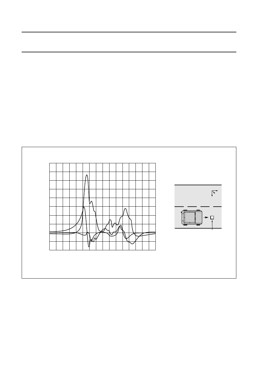
2000 Sep 06
69
Philips Semiconductors
Magnetoresistive sensors for
magnetic field measurement
General
In comparison with inductive methods, with its high
sensitivity magnetoresistive measuring can provide
information on the passing vehicle type. Also, due to the
sensor size and placement, systems can be easily and
quickly installed in any stretch of road, or even by the side
of the road, if necessary. Combined with almost negligible
power consumption, this makes magnetoresistive control
systems an inexpensive and highly efficient method of
monitoring traffic levels.
M
EASUREMENTS ON ROADS
A field test with three-dimensional sensor modules was
set-up, firstly to measure the signals of different vehicles;
and secondly, the relative occurrence of signal values of
three vehicle categories (car, van and truck). For the first
test, one module was placed in the road, under the vehicle
and for comparison, a second module was placed at the
side of the road. For the second test, which was performed
‘live’ on a street in Hamburg, Germany, the module could
only be positioned at the side of the road.
The local geomagnetic field was calibrated to zero, so that
only the disturbance in the field caused by the passing
vehicle would be recorded. Figure 39 shows the spectra
produced by an Opel Kadett.
The sensor modules also proved sensitive enough to
detect and distinguish motorbikes (even with engine,
frame and wheels being made of aluminium), which
produced the following roadside spectra.
Fig.39 Spectra for an Opel Kadett from ground sensor.
handbook, full pagewidth
MBH631
sensor-
modules
40
−
10
30
20
H
(A/m)
time
10
0
x
y
z
X
Y
Z
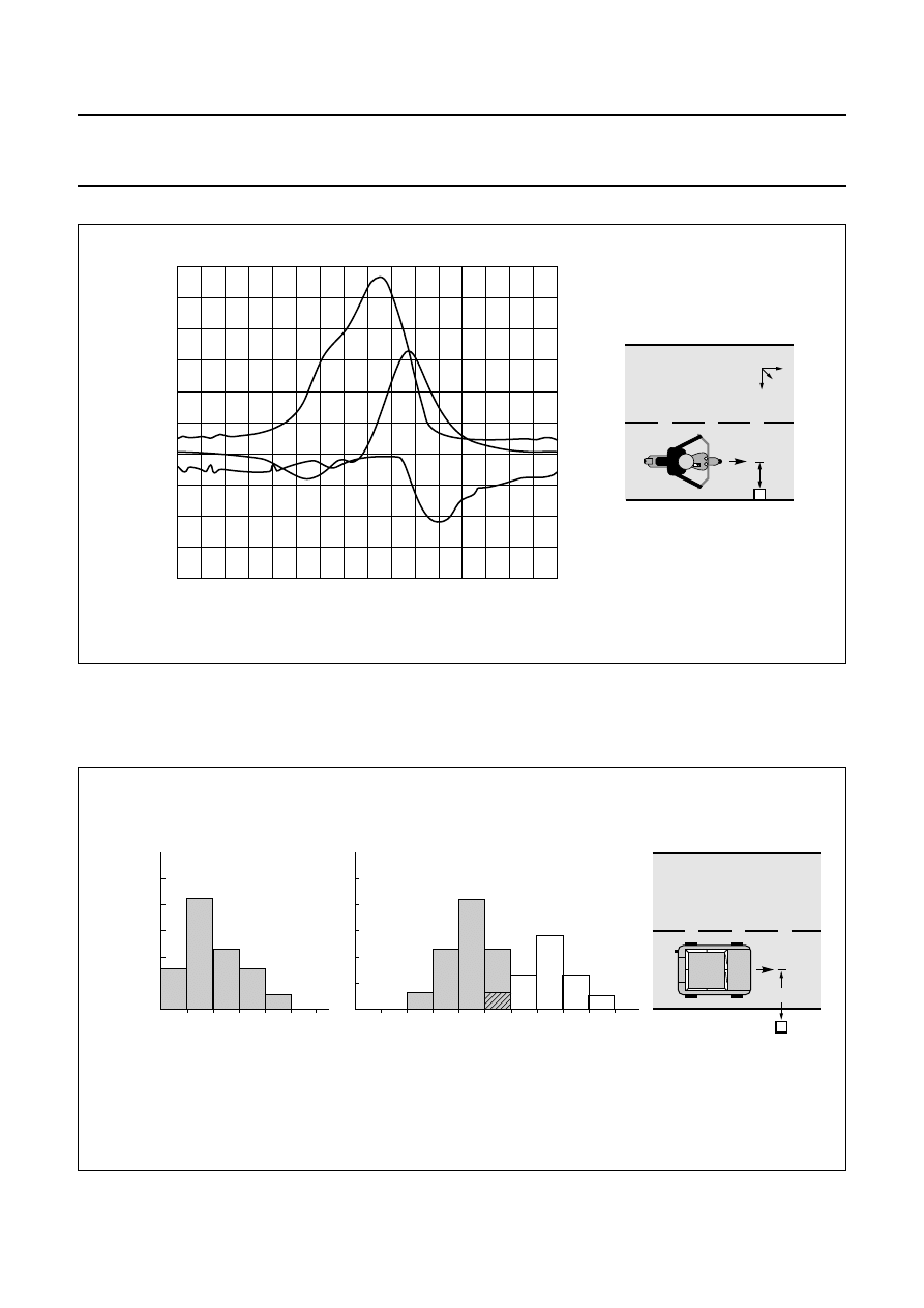
2000 Sep 06
70
Philips Semiconductors
Magnetoresistive sensors for
magnetic field measurement
General
For the roadside test in Hamburg, the road was chosen at random and the maximum signal value was recorded for
different vehicles, being grouped into cars, vans and trucks. The relative occurrence of signal values are shown in the
following diagram.
Fig.40 Spectra for a motorbike.
handbook, full pagewidth
MBH632
sensor-
modules
20 cm
6
−
4
−
2
4
2
H
(A/m)
time
0
x
y
z
X
Y
Z
Fig.41 Distribution graphs of maximum signal versus occurrence.
handbook, full pagewidth
MBH633
max. signal (A/m)
0.6
1.2
1.8
0
10
20
30
40
50
percentage
(%)
cars
max. signal (A/m)
sensor-
modules
1.2
1.8
2.4
3.0
3 m
0
10
20
30
40
50
0.6
percentage
(%)
vans
trucks (est.)
,
,
,
,,
,,
,,
,,
,,
,,

2000 Sep 06
71
Philips Semiconductors
Magnetoresistive sensors for
magnetic field measurement
General
The signals in each group seem to have a Gaussian
distribution with a characteristic maximum (although in fact
there were only three trucks, so the values for this group
are an estimate).
A
IRPORT GROUND TRAFFIC CONTROL
With the constant growth in air traffic around the world, one
serious consideration in the improvement of safety and the
ability to improve the handling capacity of airports, is the
control of traffic on and around runways. Using a traffic
control system, it is possible to introduce automatic
guidance systems and prevent runway incursions even at
heavily congested airports or under low visibility
conditions, in accordance with regulations set-down by the
internationally recognized authorities.
Although there are a number of possible sensor solutions,
traffic systems using magnetoresistive technology have
none of the drawbacks of existing radar, microwave, I/R,
pressure, acoustic or inductive systems (see Table 6).
They meet all of the functional and environmental
restraints, such as large temperature ranges, insensitivity
to climatic changes, low power consumption and, most of
all, low cost, high reliability and ruggedness. They can also
perform a range of signalling functions including detection
of presence, recognition, classification, estimation of
speed and deviation from path.
Table 6
Disadvantages of various sensors for airport ground traffic control units
Radar
Microwave barriers
Inductive sensors
•
High costs
•
Reduced efficiency with large
number of targets
•
Line of sight only
•
Complex target identification
•
Low resolution
•
Slow response times
•
Cannot be installed flush with the
ground
•
Creates new obstacles in surveyed
area
•
Produce EM interference
•
Low sensitivity and short range
•
Poor target information
•
High power consumption
•
Unreliable in harsh environments
•
Repairs require traffic to be stopped
or diverted
Pressure sensors
Acoustic sensors
I/R signalling
•
Frequent mechanical breakdowns
when used in harsh environments
•
Associated ageing problems
•
Poor target identification
•
Signal interference when used
outdoor and due to weather
conditions
•
Trade-off between sensitivity and
range
•
Large power consumption
•
Greatly affected by weather
conditions
•
Complex target identification

2000 Sep 06
72
Philips Semiconductors
Magnetoresistive sensors for
magnetic field measurement
General
EXAMPLE 3
Measurement of current
The principle of measuring current with a magnetoresistive
sensor is straightforward. As a current, i, flows through a
wire, it generates a magnetic field around it which is
directly proportional to the current. By measuring the
strength of this magnetic field with a magnetoresistive
sensor, the current can thus be accurately determined.
The relationship between magnetic field strength H,
current i and distance d is given by:
(14)
Some calculated values of H for typical conditions are
given in Table 7.
Table 7
Values for the magnetic field generated by a
current carrying wire at various distances and
currents
Table 7 clearly indicates that current measurement can
involve measurement of weak or strong magnetic fields.
As the sensitivity of magnetoresistive sensors can easily
be adjusted, using different set-ups and different
electronics (refer to the selection guide in the General
section), an individual sensor can be optimized for a
specific current measurement application, a clear
advantage over Hall effect sensors.
Set-ups with MR sensors allow current measurement
without breaking the conductor or interfering with the
circuit in any way, providing a distinct advantage over
resistor based systems. They can be used for example, for
measuring the current in a headlamp-failure detection
system in motor vehicles or in clamp-on (non-contacting)
meters, as used in the power industry.
The accuracy achievable in current measurement using
magnetoresistive sensors is highly dependent on the
specific application set-up. Factors which affect accuracy
are mechanical tolerances (such as the distance between
the sensor and the wire), temperature drift and the
sensitivity of the conditioning electronics.
In any measurement set-up, there are always other
magnetic fields present besides that generated by the
current, such as the earth’s magnetic field, and these
interfere with the measurement. A more accurate
measurement set-up uses two magnetic field sensors, to
compensate for these external fields (see Fig.43).
EXAMPLE
CURRENT
(i)
DISTANCE
(d)
MAGNETIC
FIELD (H)
1
10 mA
0.5 mm
3.18 A/m
2
1 A
0.5 mm
318 A/m
3
1000 A
10 mm
15.9 kA/m
Fig.42 Diagram showing field direction in a current
carrying wire.
handbook, halfpage
MGG423
d
H
H
i
2
π
d
----------
=
Fig.43 Diagram showing two sensors to measure
current.
handbook, halfpage
MGG426
sensor 1
sensor 2
Hdisturb

2000 Sep 06
73
Philips Semiconductors
Magnetoresistive sensors for
magnetic field measurement
General
The first sensor detects both the interference field and the
current-field in the positive direction, and the second
sensor detects the interference field in the negative
direction and the current-field in the positive direction.
These two signals are added, cancelling out the
interference field, leaving a signal that is representative of
only the current-field.
This set-up works with homogeneous interference fields
like that from the earth. Inhomogeneous fields, which will
produce different interference fields inside the two
sensors, will still affect the current measurement. This
error can be minimized by keeping the distance between
the sensors small. Large magnetic fields which fall outside
the range of the sensors can also produce errors, so the
size of external fields must be limited.
Another advantage of using two sensors, at a fixed
distance apart, is that measurement is less sensitive to
sensor-conductor distance. If the conductor is moved
closer to the first sensor, then its distance from the second
sensor is correspondingly increased and the effect is
compensated. For small differences in distance between
the conductor and sensors, sensitivity is nearly constant
and the conductor need not be fixed in place. This method
lends itself to measurement of current in free cables.
Table 8 summarizes the various advantages and
disadvantages of one-sensor and two-sensor
measurement set-ups as described above.
Table 8
Summary of advantages and disadvantages of typical measurement set-ups
CURRENT MEASUREMENT WITH TWO MAGNETIC
FIELD SENSORS
CURRENT MEASUREMENT WITH ONE MAGNETIC
FIELD SENSOR
PROS
CONS
PROS
CONS
•
no galvanic connection
•
interference effects from
inhomogeneous fields
•
no galvanic connection
•
effects of interference
from external fields
•
no breaking of the
conductor
•
errors generated from
large external fields
•
no breaking of the
conductor
•
sensitive to the
sensor-conductor
distance
•
small physical
dimensions
•
small physical
dimensions
•
reduced sensitivity to
sensor-conductor
distance
•
reduced interference
effects from
homogeneous fields
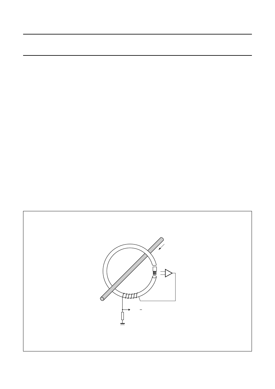
2000 Sep 06
74
Philips Semiconductors
Magnetoresistive sensors for
magnetic field measurement
General
For proper functionality of the set-ups shown in Fig.42 and
Fig.43 it is important to limit disturbing fields in x-direction
(perpendicular to sensitive direction) of the sensor. Thus
‘flipping’ of the sensor output characteristic (see section)
can be prevented.
Applications where ‘flipping’ (respectively disturbing fields
in x-direction) can not be prevented lead to a reversed
sensor characteristic. This means for one and the same
current (respectively magnetic field) the output voltage of
the MR sensor bridge can be positive or negative,
depending on the polarity of the magnetization of the
permalloy. It is obvious that this phenomenon is unwanted,
especially for DC current measurements. For AC current
measurements, flipping may cause a frequency doubling
at the output voltage of the MR sensor. This happens if the
AC current to be measured also produces periodic
magnetic field components in x-direction and therefore the
sensor is flipped periodically.
To avoid ‘flipping’ of the transfer characteristic, it must be
ensured that the magnetization of the permalloy is not
reversed by disturbing fields in x-direction of the sensor.
This can be achieved by applying a static magnetic field in
x-direction, e.g. by gluing a permanent magnet to the
sensor package. The magnitude of this stabilizing mag-
netic field in x-direction must be chosen properly,
because on the one hand magnetic fields in x-direction
avoid unwanted flipping, but on the other hand sensitivity
of the sensor is reduced (see section ’Flipping’).
A sophisticated solution for measuring DC currents, even
with the presence of disturbing magnetic fields in x-direc-
tion and therefore flipping of the output characteristic, is to
operate the sensor at its zero point. Such an arrangement
in which the magnetic field generated by the current-car-
rying wire is compensated by a secondary circuit wrapped
around a ferrite core can be seen in Fig 44.
At the ’null-field’ point, detected by the sensor located in
the air gap between the ends of the core, the magnitude of
the current in the secondary circuit is a measure of the
current in the main circuit.
Even if the sensor characteristic is reversed by disturbing
magnetic fields in x-direction then the output voltage of the
MR sensor bridge remains zero, because this operating
point is equivalent to the point where the "normal" and
"flipped" sensor characteristic intersect. Additionally this
arrangement represents a more accurate way to measure
DC currents, because any inaccuracies as a result of
mechanical tolerances, temperature drift and slight
non-linearity in the sensor characteristics are reduced.
Fig.44 Current measurement using a compensating coil.
handbook, full pagewidth
MLC141
sensor
V = I
O
R
n
ferrite
I
R
Wyszukiwarka
Podobne podstrony:
SC17 GENERAL MAG 98 1
SC17 GENERAL APP 1996 1
SC17 GENERAL TEMP 1996 3
SC17 GENERAL ROT 98 1
SC17 GENERAL TEMP 4
SC17 GENERAL ANG 1996 3
15 Sieć Następnej Generacjiid 16074 ppt
Solid Edge Generator kół zębatych
37 Generatory Energii Płynu ppt
40 0610 013 05 01 7 General arrangement
Eksploatowanie częstościomierzy, generatorów pomiarowych, mostków i mierników RLC
Biomass Fired Superheater for more Efficient Electr Generation From WasteIncinerationPlants025bm 422
Instrukcja generator sinusoidalny
Praca mag Promocja a kształtowanie wyobraźni ekonomicznej (2)
F2A GENERALMATIC
General Electric
generacja rozproszona w nowoczesnej polityce energetycznej
Generatory przebiegow niesinuso Nieznany
więcej podobnych podstron