DATA SHEET

File under Discrete Semiconductors, SC17

1997 Jan 09

DISCRETE SEMICONDUCTORS

General
Sensor systems

1997 Jan 09

2

Philips Semiconductors

Sensor systems

General

ANGLE MEASUREMENT

Contents

•

Principles and standard set-ups

•

Philips sensors for angle measurement

•

Real-life measurement applications

•

Information for advanced users and applications

– Additional measurement set-ups

– Magnets

– Angle sensor eccentricity.

Principles and standard set-ups

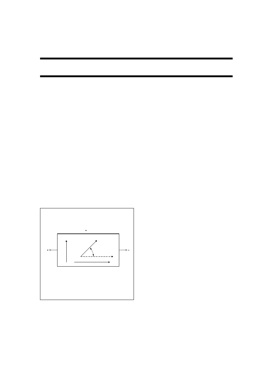
The principle behind magnetoresistive angular
measurement is essentially simple: as explained in the
general section, the MR effect is naturally an angular
effect. The resistance of the permalloy strip depends on
the angle

α

between the internal magnetization vector of

the permalloy strip and the direction of the current through
it.

When using the MR effect in sensors for measuring
angles, no linearization using a barber-pole sensor layout
Is required and the original direct relationship between the
resistance R and angle

α

(R = R

o

+

∆

R

o

cos

2

α

) is valid.

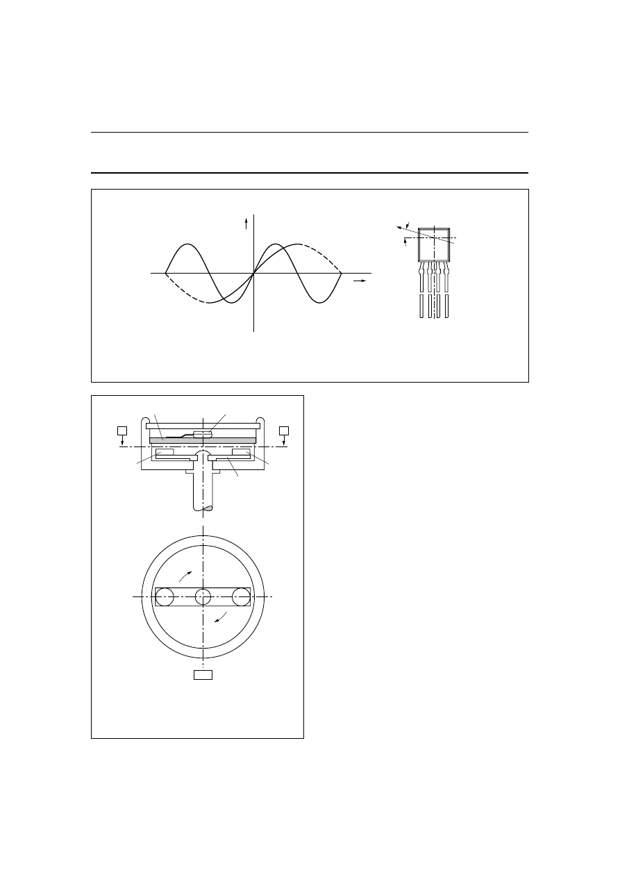
Fig.1 The magnetization effect in permalloy.

handbook, halfpage

MLC127

I

Magnetization

Permalloy

H

Current

α

R = R

∆

R cos

α

2

0

0

To achieve accurate measurement, the only condition is
that the internal magnetization vector of the permalloy
directly follows the external field. This is done by applying
an external field very much greater than the internal field
so the sensor is ‘saturated’; with today’s sensors, this is
normally achieved by having a magnetic field strength of
approximately 100 kA/m in the sensor plane. In this set-up,
(Fig.3) angle is measured directly by detecting the
field-direction and the set-up is independent of:

•

Magnet field strength

•

Magnetic drift with time

•

Magnetic drift with temperature

•

Ageing, and

•

Mechanical tolerances.

which allows for reduced system tolerances and
pre-trimming of the sensor. This is the solution adopted by
Philips in its KM110B modules. The only precaution that
need be taken with this technique is ensuring the field
directions during trimming match the field directions after
assembly.

There is ongoing development of sensors that can be
placed in this ‘saturated’ condition using steadily smaller
field strengths and this significantly reduces system costs,
because relatively inexpensive normal ferrite magnets can
be used rather than other, more costly permanent
magnets.

Note: all Philips sensors and modules have in general
been designed to be used with this ‘direct’ method.
However, there are other techniques that can be used: for
information on other methods, refer to ‘Information for
advanced users and applications’ later in this chapter

The aim in angle measurement is to influence, as fully as
possible, the internal magnetization of the sensor by the
application of an external magnetic field, so the
magnetization follows as closely as possible the external
magnetic vector. If, as recommended, a typical ‘saturation’
field of 100 kA/m is applied, due to the vector addition of
this external field with the internal magnetization of
2 kA/m, the result is a systematic error of about 2%. This
error is eliminated during the production of Philips modules
by trimming.

1997 Jan 09

3

Philips Semiconductors

Sensor systems

General

Fig.2 Internal field vectors align with a stronger

external field.

handbook, halfpage

MSB924

Hy = 0

y

x

Hy = 2 kA/m

M

M

H

Hy = 100 kA/m

M

H

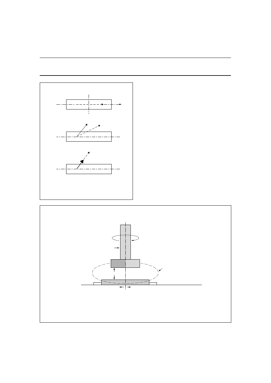
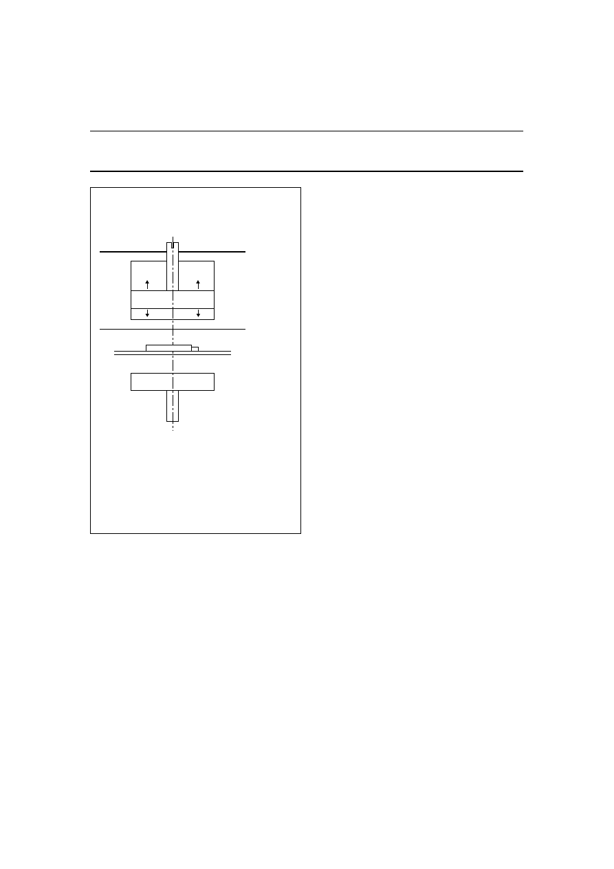
When using a sensor/magnet combination in angular
measurement applications, the magnet is placed on the
target, in front of the sensor (which is positioned so that its
internal magnetization vector is parallel to that of the
magnet at the reference point).

When the target turns, the magnet is rotated in front of the
sensor and the angle of the external field changes relative
to the internal field of the permalloy strips. This causes the
internal magnetization vector of the sensor to rotate by an
angle

α

, aligning itself with the external field (see Fig.2).

Fig.3 Arrangement of sensor and magnet.

handbook, full pagewidth

MSB927

mechanical tolerances

magnet ageing

S

N

shaft

magnet field strength

Sensing accuracy with this set-up is
unaffected by:

magnet field strength drift with time
magnet field strength drift with temperature

magnetic flux line

sensor

d

*
*
*
*
*

1997 Jan 09

4

Philips Semiconductors

Sensor systems

General

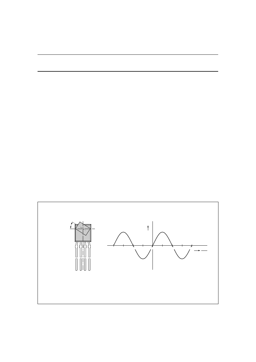
E

XTENDING ANGLE RANGE

From the basic relationship (see Appendix 1 on the
magnetoresistive effect):

(R = R

o

+

∆

R

o

cos

2

α

)

it can easily be shown that:

R

≈

sin2

α

If a sensor is used in non-linearized mode, then it
translates a single rotation of the target (360

°

) into a 720

°

output signal (2 complete sine waves). This means that
the output signal of the magnetoresistive sensor offers
good linearity only within the angle range of

±

15

°

(where

sin

α ≈ α

). If a sine wave output is acceptable in the

application (for example if there is a microprocessor in the
system which can convert the output sine curve to a linear
relationship), the angle range can to be extended to

±

35

°

(see Fig.4). Resolution is reduced at the ends of the range,
but behaviour is unaffected in the middle of the range.

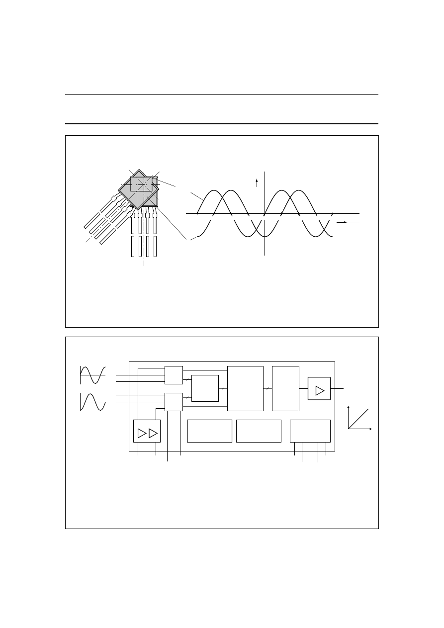
To obtain a solution for angles in the range

±

90

°

, two MR

sensors are used (see Fig.5). If they are accurately
positioned at 45

°

to one another mechanically, then

electronically their output signals are 90

°

out of phase.

Therefore the output signals from the two sensors
represent sin2

α

and cos2

α

respectively, and as

sin2

α

/cos2

α

= tan2

α

, 2

α

and therefore a can be easily

calculated.

Note: if the sensors are arranged in parallel, (positioned at
0

°

degree to one another) this set-up is excellent as a

redundant set-up (although of course the angle
measurement range will be limited). With this set-up, both
sensors are influenced equally by the external magnet, so
redundancy is achieved with only one external magnet and
the need for signal conditioning is reduced.

Although in principle the set-up in Fig.5 is simple, two
factors have to be addressed before this solution for the
measurement of angles up to 90

°

is economically viable.

Firstly, there has to be an economic way of combining
the sin2

α

and cos2

α

signals into a single signal

representing the angle

α

. To answer this need, Philips is

developing an ASIC (Fig.6) with the required signal
conditioning on one chip and offering digital interfacing
(solutions for PWM, serial bit stream and CAN.bus are now
possible).

Secondly, the sensors have to be aligned mechanically at
exactly 45

°

. This is achieved using advances in

magnetoresistive manufacturing technology, where two
overlapping sensor bridges are etched on the same
substrate, using a photo-mask process. This process has
extremely high accuracy, more than sufficient for this
application

Fig.4 Angle measurement with a KMZ10B.

handbook, full pagewidth

MBH659

−

180

45

90

135

180

0

KMZ10B

angle

deg.

signal

magnet

angle

−

45

−

90

−

135

S

N

1997 Jan 09

5

Philips Semiconductors

Sensor systems

General

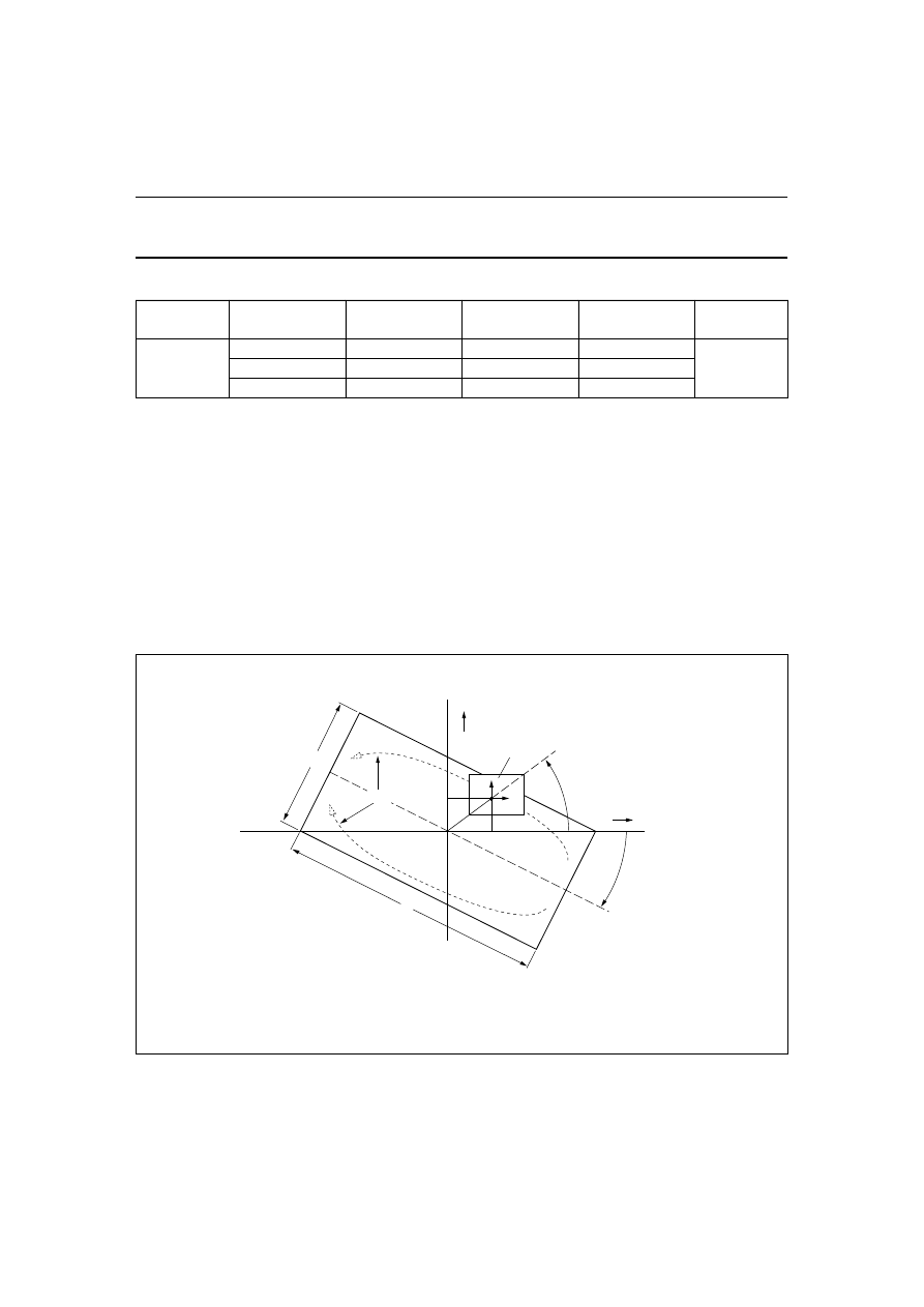
Fig.5 Angle measurement with two sensors.

handbook, full pagewidth

MBH658

−

180

45

90

135

180

0

sensor A

magnet

sensor B

A = a.sin2

α

B

= −

b.cos2

α

angle

deg.

signal

−

45

−

90

−

135

S

N

n

dbook, full pagewidth

MBH735

ALGORITHM

ADJUSTMENT

OF

OUTPUT CURVE

CHARACTERISTIC

RC-OSCILLATOR

&

CLOCK GENERATOR

BUFFER

DAC

x

14

ADC1

ADC2

14

13

13

Vout

Vout

BUFFER

−

cos(x)

sin(x)

TEST/TRIM

MODE

RESET

OFFS2

OFFS1

VIA2

VIA1

VDDA

VDD1

VSSA

VSS

VDD2

+

VO1

−

VO1

+

VO2

−

VO2

VS1

VS2

Fig.6 Block diagram of a ‘one-chip’ ASIC solution, UZZ9000.

1997 Jan 09

6

Philips Semiconductors

Sensor systems

General

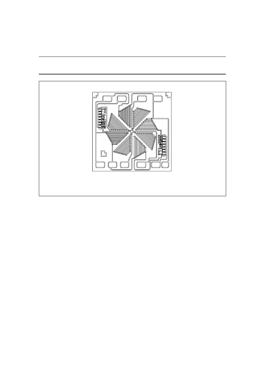
Fig.7 Layout KMZ41 chip.

handbook, full pagewidth

MBH660

1

2

1

1

2

1

2

2

Figure 7 shows the actual layout of Philips KMZ41. It has
provides 8 MR resistor networks, connected as two
individual Wheatstone bridges, aligned with a 45

°

shift in

their sensitive magnetic directions, producing the required
90

°

electrical shift.

Of course, it is also possible align both bridges
magnetically parallel to each other so they produce the
same output signal. In that case, redundancy is achieved
using a single sensor device. By increasing the number of
bridges, a combination of both principles can be achieved
to make, for example, a three-times redundant sensor or a
fully redundant sensor that can measure over the full 90

°

,

or any combination.

Philips sensor modules for angle measurement

Based on magnetoresistive sensors, Philips
Semiconductors has developed a range of ready-to-use
magnetoresistive sensor modules for contactless angle
measurement offering the following features:

•

Offset, zero point and sensitivity are pre-trimmed (so
assembly of the final encapsulated sensor is simple and
calibration after assembly is unnecessary)

•

Integrated temperature compensation; and

•

EMC protection.

These ready-to-use modules with built in signal
conditioning electronics have several advantages:

•

Output is independent of magnet tolerances,
temperature coefficients, mechanical set-up and other
tolerances

•

A single linear output signal can be provided for angles
up to 180

°

•

A variety of output signals can be provided: analog
(voltage or current), Pulse Width Modulation (PWM) and
bus interfaces (e.g. I

2

C, CAN).

Philips’ KM110BH/2xxx family is a range of modules using
hybrid thick-film technology. The circuits and magnetic
parameters of these modules have been designed so they
can be used directly in many applications, with no further
trimming or adjustment, as the basis for customized
solutions.

To reduce system costs and simplify application even
further, a family of ASIC solutions is in development, some
of which
contain both sensor and conditioning electronics. By
combining both elements in a single encapsulation,
pre-aligned systems can be offered which can be simply
mounted on a normal PCB.

1997 Jan 09

7

Philips Semiconductors

Sensor systems

General

In addition to the ready-made modules, Philips
Semiconductors is willing to undertake customised
designs for high volume applications (in excess of
50,000 units), either as specific hybrid or integrated
solutions.

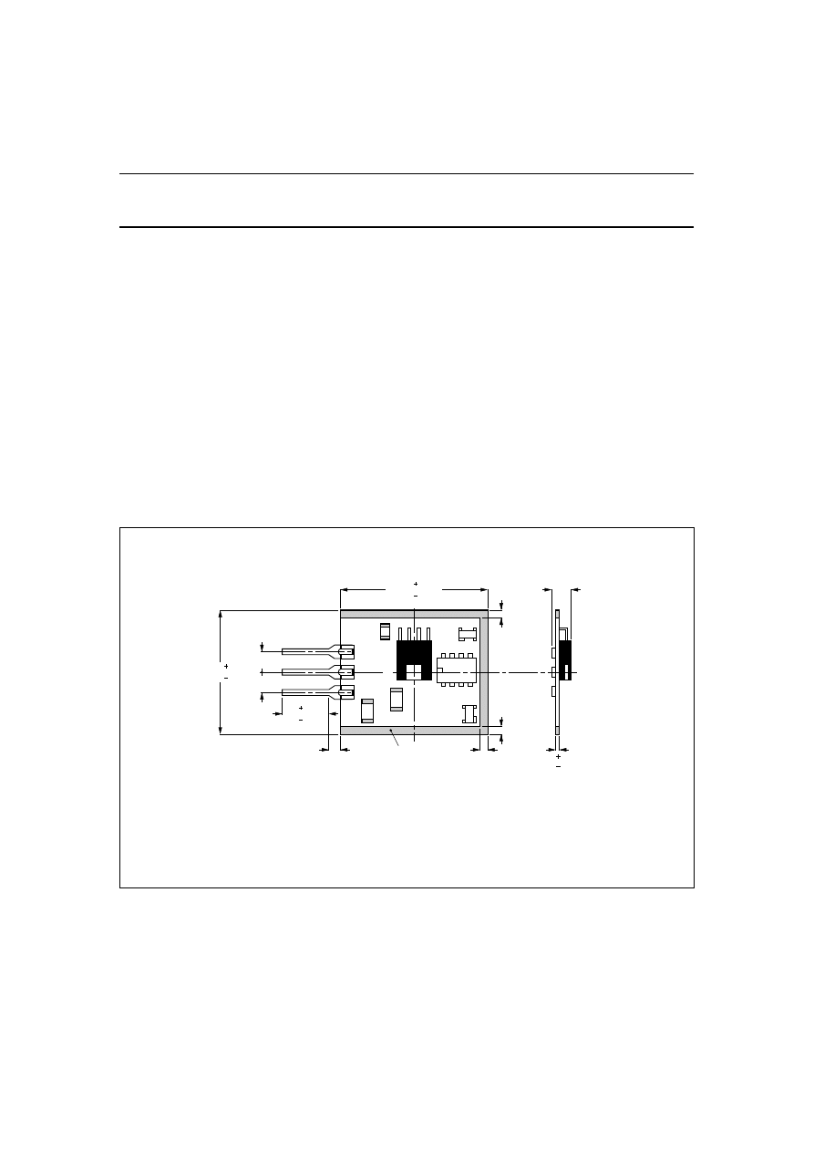
KMB110BH/21

MODULE SERIES

Figure 8 shows the construction of the KM110BH/21
module, which is based on the KMZ10B sensor and is
available in two types: the KM110BH/2130 and
KM110BH2190. They are both based on the same circuit,
but are trimmed differently: the KM110BH/2130 is trimmed
to a higher amplification and measures angles
between

−

15

°

and +15

°

, generating a linear output signal;

while the KM110BH/2190 measures angles from
approximately

−

45

°

to +45

°

and produces a sinusoidal

output. Both produce an analog voltage signal. Figure 9
shows the output V

o

of the two modules, as a function of

the measured angle

α

. For further details, refer to Table 1.

KM110BH/2270

MODULE

The KM110BH/2270 module, which is based on the
KMZ11B1 sensor, is trimmed to measure angles ranging
from

−

35

°

to +35

°

and has integrated input voltage

stabilization. In contrast to the other modules in the
KM110BH/2 range, the KM110BH/2270 has an analog
current output signal (4 to 20 mA), which can be converted
to a voltage signal using a simple resistor. The output is
sinusoidal. This module has extremely good resolution
and reproducibility (better than 0.001

°

at

α

= 0

°

) and

hysteresis, which is typically 0.02

°

at a = 0

°

, is very low.

When designing an encapsulation for the KM110BH/2270,
it may be necessary to have the pins of the hybrid bent into
an ‘S’ shape, to avoid excessive force on the solder joints.
In this case, please order the KM110BH/2270G. For
further details, refer to Table 1.

Fig.8 Construction of a KM110BH/21.

handbook, full pagewidth

MBC703

VCC

mounting rim

GND

VO

2.54

2.54

19.05

0.25
0.05

3.2

max

0.25
0.05

16.933

standoff = 1

0.8 min

0.8

min

0.8

min

0.5
0.5

6

0.08
0.08

0.76

1997 Jan 09

8

Philips Semiconductors

Sensor systems

General

Table 1

An overview of the main characteristics of Philips modules for angle measurement

PARAMETER

KM110BH

UNIT

2130

1

2190

2

2270

2430

2470

Angle range

30

90

70

30

70

deg

Output voltage

3

0.5 to 4.5

0.5 to 4.5

−

0.5 to 4.5

0.5 to 4.5

V

Output current

−

−

4 to 20

−

−

mA

Output characteristic

linear

sinusoidal

sinusoidal

linear

sinusoidal

−

Supply voltage

5

5

5

5

5

V

Substrate dimensions

9.1

×

16.9

9.1

×

16.9

23.6

×

20.3

23.6

×

20.3

23.6

×

20.3

mm

Resolution

0.001

0.001

0.001

0.001

0.001

deg

Temperature range

−

40 to +125

−

40 to +125

−

40 to +125

−

40 to +125

−

40 to +125

°

C

Fig.9 Output characteristics of the KM110BH/2130 and KM10BH/2190 modules.

handbook, full pagewidth

α

KM110BH/2190, measurement

MBC705

15

45

45

15

α

(deg)

4.5 V

2.5 V

0.5 V

output signal

VO

V = 5 V

CC

VO

GND

VCC

d

external

magnet

range is 90

KM110BH/2130, measurement

range is 30

N

S

1997 Jan 09

9

Philips Semiconductors

Sensor systems

General

KM110BH/24

MODULE

The KM110BH/24 is available in two versions based on the
KMZ41: the KM110BH/2430 is trimmed to
measure angles between

−

15

°

and +15

°

, generating a

linear output signal (non-linearity is

≈

1%); while the

KM110BH/2490 measures angles from approximately

−

35

°

to +35

°

and produces a sinusoidal output. On-board

protection circuitry makes these modules EMC tolerant.

Real-life angular measurement applications

With angular measurement using magnetoresistive
sensors, the number of possible applications is very broad,
replacing
and outperforming other types of sensors in a variety of
applications, some of which are listed in Table 2:

Amongst these numerous applications, undoubtedly the
most common is in the automotive industry, where they are
used to measure pedal and throttle position.

R

EDUNDANT SYSTEMS

As multiple sensors with identical behaviour can be
implemented on a single piece of silicon, a
magnetoresistive set-up is an ideal solution for the
construction of redundant systems, in safety critical
applications, for example, such as a car accelerator pedal.

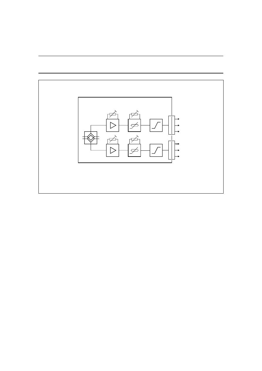
The essential functional blocks of a typical redundant
sensor system are shown in Fig.10. For each sensor, the
signal is first amplified. This stage also includes offset
compensation and determines the characteristic of the
output signal (sinusoidal or linear). After temperature
compensation, the third stage provides additional trimming
of the output signal and allows for the inclusion of
diagnostic functions (for example, wire not connected or
short circuit conditions). The final stage provides additional
protection, against short circuits (between the supply
voltage and the output signal, for example) or overvoltage
(for example, if the 5 V module supply is accidentally
connected to a 14 V battery supply).

Table 2

Typical applications for angle sensors

Automotive and agricultural

Industrial

•

Pedal position

•

Active suspension units

•

Self-levelling systems

•

Automatic headlight adjustment

•

Valve control

•

Material thickness

•

Feedback systems for belt control

•

Wear detection

Medical

Consumer

•

Body and brain scanners where accurate angle
information is vital to build up cross-sectional images

•

Control joysticks for tilting tables

•

Games joysticks

•

Spirit levels

1997 Jan 09

10

Philips Semiconductors

Sensor systems

General

Fig.10 Functional block diagram of module with redundancy.

handbook, full pagewidth

MSB923

redundant

sensor

offset compensation

trimming of signal

characteristic

temperature

compensation

signal

conditioning

GND (1)

VCC (1)

VO (1)

GND (2)

VCC (2)

VO (2)

Information for advanced users and applications

A

DDITIONAL MEASUREMENT SET

-

UPS

Linear

In linear angle measurement, the strength of the external
magnetic field used is within normal sensitivity levels and
the sensor measures the resulting field strength of the
rotating magnet. As can be seen from Fig.11, the signal
linearity of a weak field method allows for angles up to

±

90

°

to be measured without correction for the sinusoidal

shape of the wave. This is the technique used in most
competing angle measurement set-ups. However, since
the magnet’s properties directly influence sensor output,
the measurement equipment must be carefully calibrated
after it is assembled and calibration for material ageing is
not possible at all. Only with a very well defined magnetic
system can a pre-calibrated circuit be used and defining
such a system is difficult and expensive, due to the
tolerances caused by the thermal sensitivity of the magnet
and the mechanical set-up.

By using a set-up with two magnets placed on a rotatable
frame, angular rotations of around

±

85

°

can be measured

and through the symmetrical positioning of the magnets,
the effect of the magnet position is eliminated. Figure 12
shows a practical arrangement, which basically acts as a
contactless potentiometer. However, the response is not a
perfectly sinusoidal due to magnetic influences on the ‘x’
and ‘y’ axis.

1997 Jan 09

11

Philips Semiconductors

Sensor systems

General

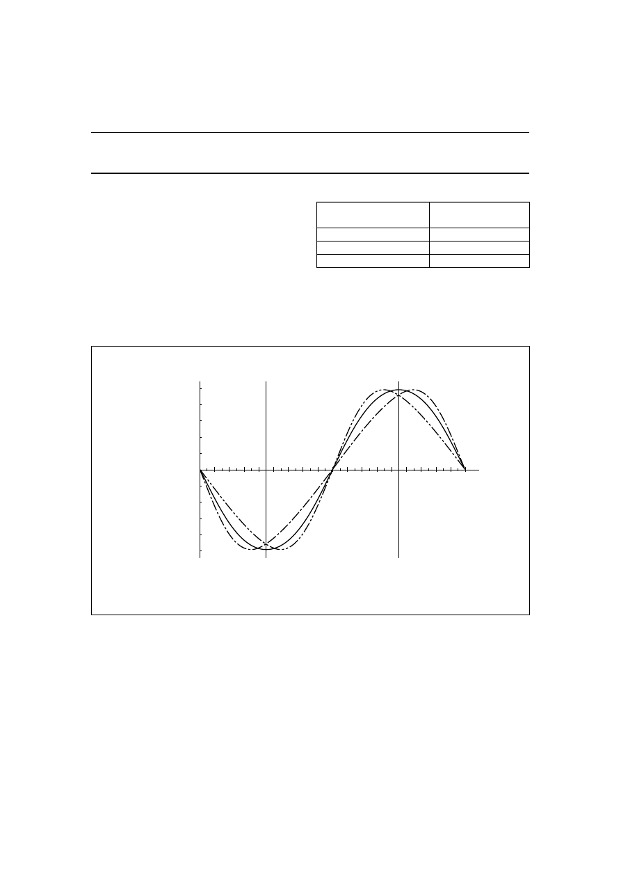
Fig.11 Sensor response for different magnetic fields.

handbook, full pagewidth

MBH716

1

2

3

4

α

H

KMZ10

signal

α

/degrees

strong field H

weak field H

Fig.12 Contactless potentiometer for angle

measurement.

,,,,,,,

,,,,,,,

,,,,,,,

,,,,,,,

,,,,,,,

,,,,,,,

,,,,,,,

,,,,,,,

handbook, halfpage

MBH651

,,,,

,,,,

,,,,

,,,,

,,,

,,,

,,,

,,,

,,,,

,,,,

A

B

A - B

KMZ10C

substrate

magnet

RES190

magnet

RES190

steel

S

α

α

N

1997 Jan 09

12

Philips Semiconductors

Sensor systems

General

Fig.13 Angle sensor with adjustable measuring range.

handbook, halfpage

,,,,,,,,

,,,,,,,,

,,,,,,,,

,,,,,,,,

,,,,,,,,

MBH656

adjustment mechanism
e.g. screw

plain bearing

adjustment magnet

substrate

moved magnet

axis of rotation

sensor

,,,,

,,,,

,,,,

Extending measurement angle to greater than 90

°

With a second fixed magnet, it is possible to adjust the
sensing distance and the angle range can be further
extended, to cope with angles greater than

±

90

°

. This can

lead to increased mechanical tolerances although by using
magnets of the same material, temperature variations can
be disregarded. Figure 13 shows a typical set-up.

M

AGNETS

The main requirement for the magnet is that it should be
strong, to ensure all tolerances are negligible, but
obviously cost and space must also be considered,
according to individual application requirements. Table 3
compares three commercially available Samarium-Cobalt
(SmCo) magnets suitable for angle measurement
applications.

These magnets have a tolerance in their magnetization
direction which affects angle measurement. This
tolerance, which can be up to 2%, should be taken into
account if no mechanical calibration is possible at

α

= 0

°

.

The symmetry axis of the module and the rotation axis of
the magnet should be identical, although if one of the axes
is shifted slightly, the affect on sensing accuracy can be
neglected because the field lines of the magnet are
parallel. Measurements with magnets with a face of
11.2

×

8 mm oriented towards the sensor allow for

eccentric tolerances of up to 0.5 mm, assuming an
acceptable tolerance in V

o

of 1%; and up to 0.25 mm, for

an acceptable tolerance in V

o

of 0.5%. Evidently, if the

magnet is smaller, these values should be proportionately
reduced.

1997 Jan 09

13

Philips Semiconductors

Sensor systems

General

Table 3

Typical values for various dimensions of Sm

2

Co

17

magnets

MATERIAL

DIMENSIONS

(1)

(mm)

d

(2)

(mm)

TOLERANCE d

(3)

(mm)

ECCENTRICITY

(4)

(mm)

T

amb

(

°

C)

Sm

2

Co

17

11.2

×

5.5

×

8

2.1

±

0.30

±

0.25

−

55 to + 125

6

×

3

×

5

0.7

±

0.15

±

0.15

8

×

3

×

5

0.5

±

0.30

±

0.20

Notes

1. Magnetization is always parallel to the latter

dimension.

2. d’ is the distance between the magnet and the front of

the sensor.

3. Tolerance’ is the maximum deviation in ‘d’ for which

the change in sensor output signal is <0.5% of full
scale output.

4. Eccentricity’ is the maximum deviation of the magnet

rotational axis from the sensor rotational axis for which
the change in sensor output signal is <0.5% of full
scale output.

A

NGLE SENSOR ECCENTRICITY

In angle measurement using the direct measurement
technique, the ideal arrangement is with a homogeneous
parallel field. Although large magnets fulfil this
requirement, there is usually a compromise between
magnet size and the corresponding tolerances of the
sensor due to cost considerations.

If the sensor and the magnet rotation axes are in line, the
sensor output characteristics follow approximately the
following
signal voltage relationship:

V

o

= V

o

(0)

×

sin2

α

Fig.14 Angle sensor with eccentric sensor position.

handbook, full pagewidth

MBH655

W

I

S

S

N

N

α

Y

Ym

Rm

Xm

X

−

Hy

Hx

sensor

magnet

δ

field lines

1997 Jan 09

14

Philips Semiconductors

Sensor systems

General

However, depending on the sensor position in relation to
the magnet and the angle to be measured (see Fig.14),
offsets or sensitivity changes can occur. These conditions
alter the ideal relationship as described by the equation
above.Angle tolerance values can be calculated using the
following relationship:

∆α

= C

×

R

m

2

×

sin2(

α

+

δ

)

C is a magnetic constant and, provided the width and
length of the magnet are approximately equal, can be
calculated from the following equation:

C

320

w

l

+

(

)

2

---------------------

=

Table 4

Typical values of C for Sm

2

Co

17

magnets

For positions on the x- and y-axis, there is a sensitivity
change with a maximum tolerance level at

α

=

±

45

°

and

±

135

°

(see Fig.15); for diagonal positions, an offset

tolerance occurs with a maximum at

α

=

±

90

°

and

±

180

°

(see Fig.16).

MAGNET DIMENSIONS

(w

×

h

×

l, mm)

C

(degree/mm

2

)

6

×

3

×

5

2.6

8

×

3

×

7.5

1.35

11.2

×

5

×

8

0.74

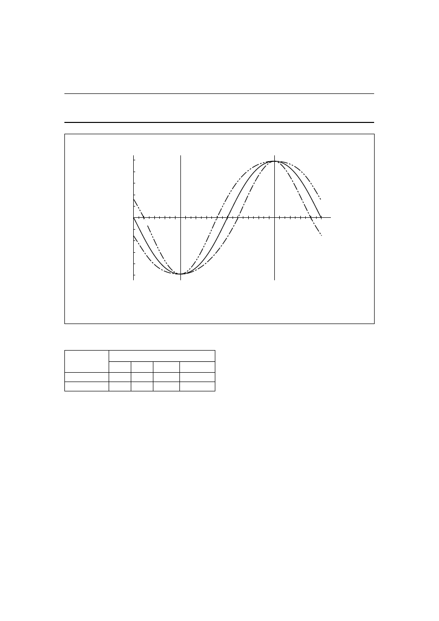
Fig.15 Response tolerances for sensor position on x- and y-axes.

handbook, full pagewidth

MBH654

−

60

−

40

−

20

0

20

40

60

80

−

0.2

−

0.4

−

0.6

−

0.8

−

1.0

1.0

0.8

0.6

0.4

0.2

0

V0/V0

(O)

δ

= 0

°

/180

°

δ

= 90

°

/

−

90

°

−

80

α

/

°

1997 Jan 09

15

Philips Semiconductors

Sensor systems

General

Fig.16 Response tolerances for sensor position diagonals.

handbook, full pagewidth

MBH653

−

60

−

40

−

20

0

20

40

60

80

−

0.2

−

0.4

−

0.6

−

0.8

−

1.0

1.0

0.8

0.6

0.4

0.2

0

V0/V0

(O)

δ

= 45

°

/

−

135

°

δ

= 45

°

/135

°

−

80

α

/

°

Table 5

Typical tolerance values of

∆α

for

C

×

R

m

2

= 1

Single sensor system

If we assume that a single, encapsulated angle sensor with
eccentricity will be adjusted mechanically to the specified
output voltage V

o

(

α

= 0), then the tolerances at

α

= 0 are

set to zero. Then over the useful angle range of

±

45

°

, the

original offset tolerances can be transformed into a
resultant

∆α

tolerance:

∆α

= 2C

×

R

m

2

sin

2

α

∆α

(DEGREES)

∆

(DEGREES)

0

15

30

45

0/90/...

0

0.5

0.87

1

45/135/...

0

0.134

0.25

1

Some typical values when C

×

R

m

2

= 1 are shown in

Table 5.

An adjusted 30

°

angle sensor has a maximum tolerance

of:

∆α =

1

⁄

2

CR

m

2

at

±

15

°

and in the range between 0

°

and 15

°

, the tolerance

increases approximately linearly from zero to this value.
Above

±

15

°

the sinusoidal function given above is effective

and has to be taken into account for the 70

°

and 90

°

sensors.

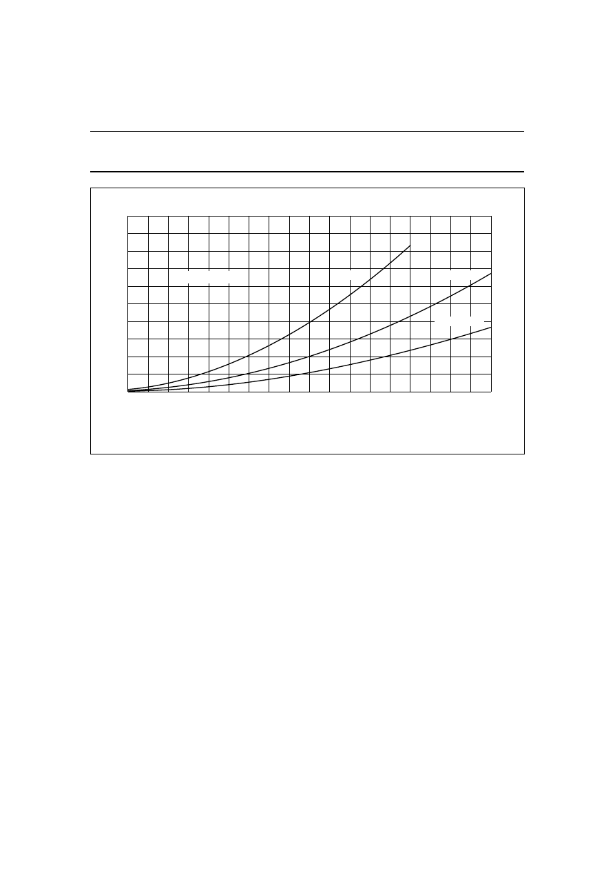
Figure 17 gives the maximum tolerances at

α

=

±

15

°

for

different magnets as a function of the eccentricity
radius R

m

.

In general, the tolerance is about 0.3

°

or 1% FS,

provided R

m

corresponds to about 10% of the magnetic

dimensions l and w.

1997 Jan 09

16

Philips Semiconductors

Sensor systems

General

Fig.17 Maximum angle tolerances

∆α

.

handbook, full pagewidth

0.8

0.9

Rm/mm

1.0

1.0

0

0.1

0.2

0.7

0.3

0.4

|

∆α

|/

°

0.5

0.6

0.2

0.4

0.6

0.8

MBH652

Sm

2

Co

17

-magnets

6, 3, 5 mm

3

8, 3, 7.5 mm

3

11.2, 5.5, 8 mm

3

Double sensor system (KMZ41)

In this case, both sensors are influenced differently and the
resulting tolerance

∆α

has to be calculated from the

deviations of the two response curves. If C.Rm2 is
sufficiently small, and the angle a is calculated from the
relation of the two output signals via the arc-tan function,
then the resulting measuring tolerance can be described
by:

∆α

= C

×

R

m

2

×

cos4

α ×

sin2(

α

+

δ

)

This leads to the worst case tolerance of

∆α

= C

×

R

m

2

occurring at

α

= 0

°

, 45

°

and 90

°

and a tolerance of zero at

α

= 22.5

°

, 67.5

°

and 112.5

°

. These zero positions can be

used to adjust the sensor for the highest precision
measurements.

If the sensors are adjusted in this way, the maximum
tolerance is limited to C

×

R

m

2

.