ENVI Tutorial:
Atmospherically Correcting
Hyperspectral Data Using
FLAASH

Overview of This Tutorial

2

Files Used in This Tutorial

2

Opening the Uncorrected AVIRIS Image

3

Atmospherically Correcting the AVIRIS Image Using FLAASH

5

Viewing the Corrected Image

7

Comparing Images

7

References

8

1

Overview of This Tutorial

This tutorial provides an introduction to using FLAASH to atmospherically correct a hyperspectral
image. You will display the radiance image, apply an atmospheric correction, and examine the results.

Note: The Atmospheric Correction Module: QUAC and FLAASH requires an additional license for
your ENVI installation; contact your ITT Visual Information Solutions sales representative to purchase
a license.

Files Used in This Tutorial

The image used in this exercise was collected by the Airborne Visible Infrared Imaging Spectrometer
(AVIRIS) sensor, which is operated by NASA. The sample image covers a portion of the Jasper Ridge
Biological Preserve, located in the eastern foothills of the Santa Cruz Mountains at the base of the San
Francisco Peninsula, 9 km west of the Stanford University campus in San Mateo County, California. The
AVIRIS data were provided courtesy of the NASA Jet Propulsion Laboratory (JPL) in Pasadena,
California. For more information about the sample data, see the file FLAASH_Sample_Data_
Readme.txt in the Data\flaash\hyperspectral\ancillary_data directory. This image
contains approximately the same area as the Landsat TM image used for the multispectral FLAASH
tutorial; however, the pixel size, image orientation, and collection dates are different.

All files are on the ENVI Resource DVD.

Data\flaash\hyperspectral\input_files

File

Description

JasperRidge98av.img (and .hdr) AVIRIS radiance image and header file

AVIRIS_1998_scale.txt

Scale factors file for the AVIRIS data

JasperRidge98av_template.txt

Template file

The files in the directory Data\flaash\hyperspectral\flaash_results are for
verification purposes only and are not required for this tutorial.

2

ENVI Tutorial: Atmospherically Correcting Hyperspectral Data
Using FLAASH

ENVI Tutorial: Atmospherically Correcting Hyperspectral Data

Using FLAASH

Opening the Uncorrected AVIRIS Image

This exercise will demonstrate how to use FLAASH to produce an apparent surface reflectance image.

1. From the ENVI main menu bar, select File > Open Image File. The Enter Data Filenames dialog

appears.

2. Navigate to Data\flaash\hyperspectral\input_files, and select

JasperRidge98av.img. Click Open. The Available Bands List appears.

3. In the Available Bands List, right-click on JasperRidge98av.img and select Load True

Color. The image is loaded into a display group.

You may recognize several features in the scene, including a vertically oriented lake in the top
center of the image, various types of vegetation in the left side of the image, and urban areas in
the right side of the image. This image is a standard AVIRIS data product that JPL processed. It
contains calibrated at-sensor radiance values that were scaled into 2-byte signed integers.

4. Right-click in the Image window and select Z Profile (Spectrum) to display the Spectral Profile

plot window.

5. Move the Image box (inside the Image window) around the image and note how the shape of the

radiance curve automatically updates in the Spectral Profile window.

6. Right-click in the Image window and select Pixel Locator.

7. Move the Pixel Locator so that you can see it and the Spectral Profile window at the same time.

8. In the Pixel Locator, enter 366 and 179 in the Sample and Line fields, respectively. Click Apply

to center on this pixel location, which illustrates some of the common atmospheric features often
seen in hyperspectral data:

3

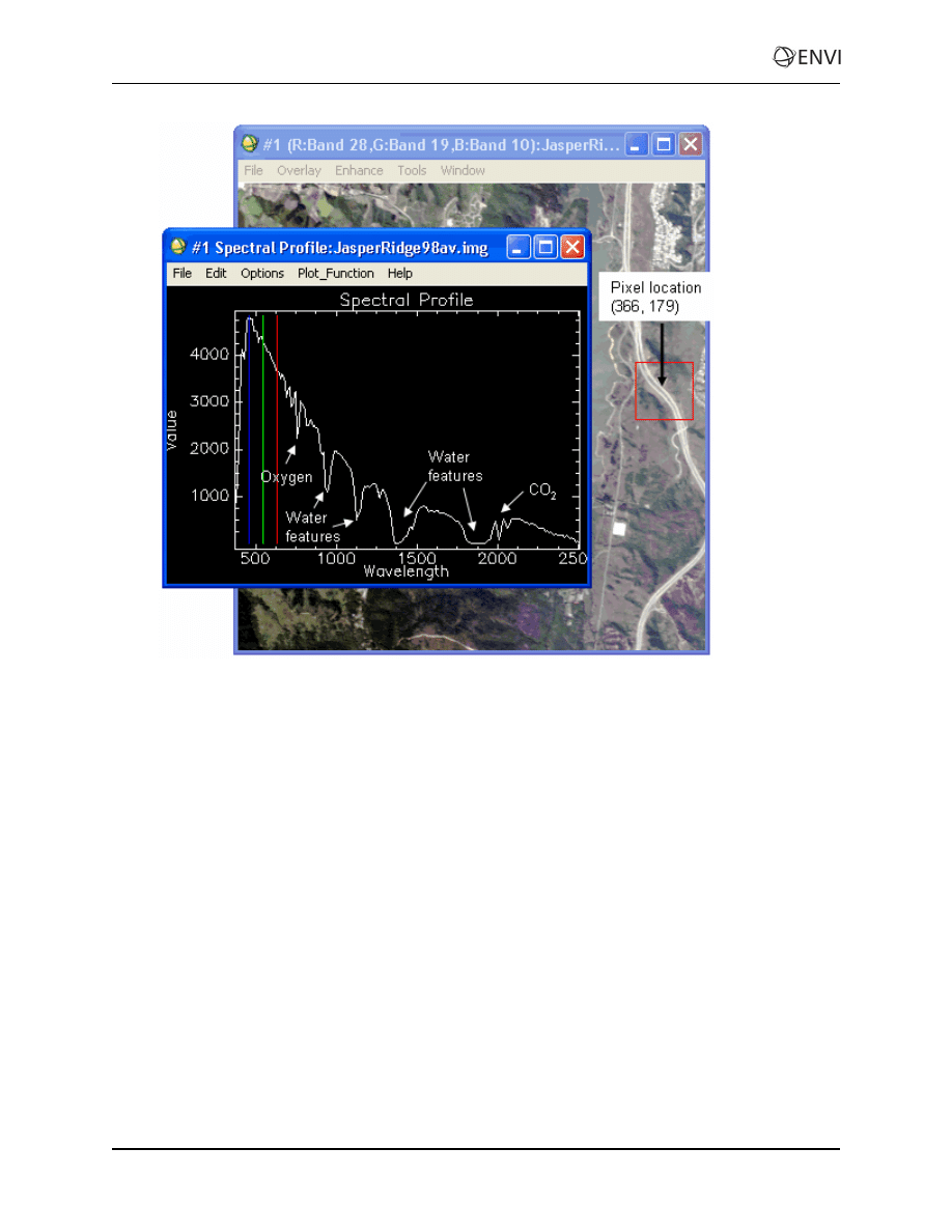
9. Click and drag the cursor in the Spectral Profile window along the radiance spectrum, and locate

the water vapor absorption features at approximately 760 nm, 940 nm, and 1135 nm. Note also the
opaque atmospheric regions around 1400 nm and 1900 nm where virtually no signal is recorded at
the instrument. You can also see a common CO

2

signature that consists of two absorption

features near 2000 nm.

10. Keep the display group and Spectral Profile open for the next exercise.

4

ENVI Tutorial: Atmospherically Correcting Hyperspectral Data
Using FLAASH

ENVI Tutorial: Atmospherically Correcting Hyperspectral Data

Using FLAASH

Atmospherically Correcting the AVIRIS Image
Using FLAASH

1. From the ENVI main menu bar, select Spectral > FLAASH. The FLAASH Atmospheric

Correction Model Input Parameters dialog appears.

2. Click Input Radiance Image. The FLAASH Input File dialog appears.

3. Select the file JasperRidge98av.img, and click OK. The input radiance image consists of

2-byte signed integer values. For FLAASH to compute the atmospheric correction, these data
values must be converted into floating-point radiance values in units of

μW / (cm2 * nm * sr). In the next few steps, you will restore a scale factor file that will convert

the values to floating point.

4. In the Radiance Scale Factors dialog, select the Read array of scale factors (1 per band) from

ASCII file radio button, and click OK. The file selection dialog appears.

5. Navigate to Data\flaash\hyperspectral\input_files, select the file AVIRIS_

1998_scale.txt, and click Open. The Input ASCII File dialog appears.

6. Accept all of the default values, and click OK.

The 1998 AVIRIS scale factors (which are valid for all AVIRIS data collected between 1995 and
2003) are 500 for the first 160 bands and 1000 for the remainder.

In the FLAASH Atmospheric Correction Model Input Parameters dialog, the default path and
filename for the reflectance output are displayed in the Output Reflectance File field.

7. In the Output Reflectance File field, type the full path of the directory where you want to write

the output reflectance file. For the filename, type JasperRidge98av_flaash.img. To navigate to
the desired output directory before defining the output filename, click the Output Reflectance
File button.

8. In the Output Directory for FLAASH Files field, type the full path of the directory where you

want to write all other FLAASH output files. You may also click the Output Directory for
FLAASH Files button to navigate to the desired directory.

9. In the Rootname for FLAASH Files field, type a root name that will be added as a prefix to the

FLAASH output files. In the next step, ENVI will automatically add an underscore character to
the root name that you enter.

FLAASH output files consist of a column water vapor image, cloud classification map, journal
file, and (optionally) a template file. All files are written to the FLAASH output directory, and the
root name is added as a prefix to the individual standard filenames.

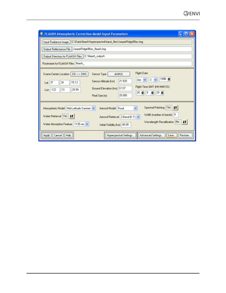
10. Click the Restore button, located on the bottom right of the FLAASH Atmospheric Correction

Model Input Parameters dialog.

11. Navigate to Data\flaash\hyperspectral\input_files, select the file

JasperRidge98sav_template.txt, and click Open. This file provides some scene
information for the AVIRIS image, along with FLAASH model parameters. The FLAASH
Atmospheric Correction Model Input Parameters dialog should look similar to the following.

5

12. Click Advanced Settings at the bottom of the dialog to explore the advanced options that are

available. The parameters in the Advanced Settings dialog allow you to adjust additional controls
for the FLAASH model.

The default setting for Automatically Save Template File is Yes, and the default for Output
Diagnostic Files is No. While you may find it excessive to save a template file for each
FLAASH run, the template file is the only way to determine the model parameters that were used
to atmospherically correct an image after the run is complete, so it is important to be able to
access it. The ability to output diagnostic files is offered solely as an aid for ITT Visual
Information Solutions Technical Support to help diagnose problems.

13. Click Cancel to dismiss the Advanced Settings dialog.

14. In the FLAASH Atmospheric Correction Model Input Parameters dialog, click Apply to begin

FLAASH processing. You may cancel the processing at any point, but be aware that there are
some FLAASH processing steps that cannot be interrupted, so the response to the Cancel button
may not be immediate.

6

ENVI Tutorial: Atmospherically Correcting Hyperspectral Data
Using FLAASH

ENVI Tutorial: Atmospherically Correcting Hyperspectral Data

Using FLAASH

Viewing the Corrected Image

When FLAASH processing is complete, the output reflectance image, column water vapor image, and
cloud classification map, are added to the Available Bands List. You should also see the journal file and
template file in your FLAASH output directory.

1. Click Cancel in the Atmospheric Correction Model Input Parameters dialog to dismiss the dialog.

2. Examine, then close, the FLAASH Atmospheric Correction Results dialog.

3. From the Available Bands List, right-click on JasperRidge98av_flaash.img (the

reflectance file you just created), and select Load True Color to <New>. The image is loaded
into a new display group.

Comparing Images

In the following steps, you will compare the Z Profile values of the uncorrected radiance image with the
FLAASH-corrected reflectance image. You should already have the display group and Spectral Profile
open from the original radiance image.

1. Right-click in any of the two Image windows and select Link Displays. The Link Displays dialog

appears.

2. Ensure that Display #1 and Display #2 both say Yes, and click OK.

3. Right-click in the Image window for Display #2 (reflectance image), and select Z Profile

(Spectrum).

4. In the Image window for Display #2, click and drag around the image and note the shape of the

reflectance curves. Note that some bands in the reflectance image have been designated as ENVI
"bad" bands and are not displayed in the plot window. The bad bands list in the ENVI header file
is automatically set by FLAASH according to the strength of the reflectance signal.

5. Right-click in any Image window and select Pixel Locator. The Pixel Locator dialog appears.

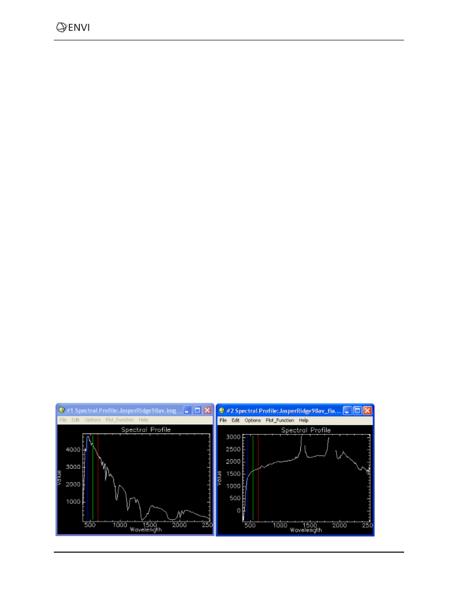
6. Enter 366 and 179 in the Sample and Line fields, respectively. Click Apply. Compare the shape

of the radiance curve (#1 Spectral Profile) with the shape of the reflectance curve (#2 Spectral
Profile) for the same pixel location. This is one way to verify that the atmospheric correction was
successful.

7

References

Abreau, L. W., and G. P. Anderson, eds. The MODTRAN 2/3 Report and LOWTRAN 7 Model. Air Force
Research Laboratory, Hanscom AFB, MA. 01731-3010, prepared by Ontar Corp. under Contract No.
F19628-919C-0132. January 1996.

Kaufman, Y. J., A. E. Walk, L. A. Refer, B.-C. Gao, R. -R. I, and L. Fling. The MODIS 2.1-mm
Channel--Correlation with Visible Reflectance for Use in Remote Sensing of Aerosol. IEEE
 Transactions on Geosciences and Remote Sensing, Vol. 35, pp. 1286-1298. 1997.

8

ENVI Tutorial: Atmospherically Correcting Hyperspectral Data
Using FLAASH