Introduction to the Numerical Solution of IVP for ODE
45
Introduction to the Numerical Solution of IVP for ODE
Consider the IVP: DE x
′
= f (t, x), IC x(a) = x
a
. For simplicity, we will assume here that
x(t) ∈ R
n
(so F = R), and that f (t, x) is continuous in t, x and uniformly Lipschitz in x
(with Lipschitz constant L) on [a, b] × R
n
. So we have global existence and uniqueness for
the IVP on [a, b].
Moreover, the solution of the IVP x
′
= f (t, x), x(a) = x
a
depends continuously on the
initial values x
a
∈ R
n
. This IVP is an example of a well-posed problem: for each choice of
the “data” (here, the initial values x
a
), we have:
(1) Existence. There exists a solution of the IVP on [a, b].
(2) Uniqueness. The solution, for each given x
a
, is unique.
(3) Continuous Dependence. The solution depends continuously on the data.
Here, e.g., the map x
a
7→ x(t, x
a
) is continuous from R
n
into (C ([a, b]) , k · k
∞
). A well-posed
problem is a reasonable problem to approximate numerically.
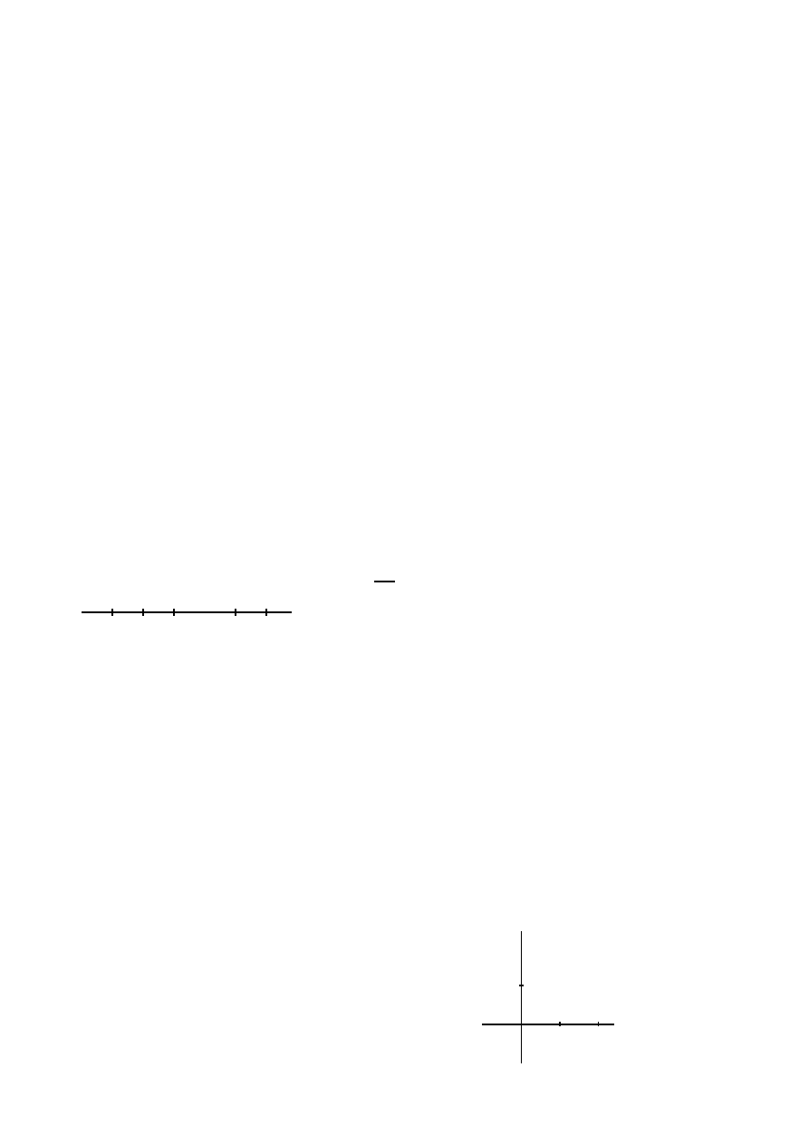
Grid Functions
a
t
1
t
2
· · · t
N
b
t
0
t
z}|{z}|{
h
h
Choose a mesh width h (with 0 < h ≤ b − a), and let
N =
b−a
h
(greatest integer ≤ (b−a)/h). Let t
i
= a + ih
(i = 0, 1, . . . , N) be the grid points in t (note: t
0
= a),
and let x
i
denote the approximation to x(t
i
). Note that
t
i
and x
i
depend on h, but we will usually suppress this
dependence in our notation.
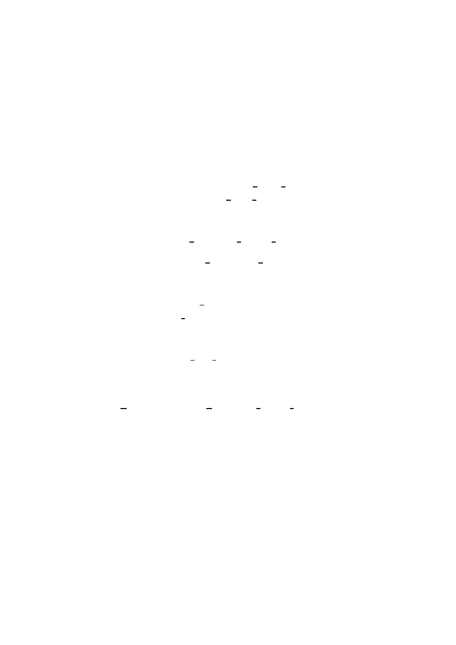
Explicit One-Step Methods
Form of method: start with x
0
(presumably x
0
≈ x
a
). Recursively compute x
1
, . . . , x
N
by
x
i+1
= x
i
+ hψ(h, t
i
, x
i
),
i = 0, . . . , N − 1.
Here, ψ(h, t, x) is a function defined for 0 ≤ h ≤ b−a, a ≤ t ≤ b, x ∈ R
n
, and ψ is associated
with the given function f (t, x).
Examples.
x
i
t
i
t
i+1
x
t
s
.
..
..
..
..
..
..
..
..
..
..
..
..
..
..
..
..
..
..
..
..
..
..
..
..
..
..
..
..
..
..
..
.
..
..
..
..
..
..
..
..
..
..
..
..
..
..
..
..
..
..
..
..
..
..
..
..
..
..
..
..
..
.
..
..
..
..
..
..
..
..
..
..
..
..
..
..
..
..
..
..
..
..
..
..
..
..
..
..
..
..
..
..
solution through
(ti,x9)
tangent line
x
i+1
Euler’s Method.
x
i+1
= x
i
+ hf (t
i
, x
i
)
Here, ψ(h, t, x) = f (t, x).

46
Ordinary Differential Equations
Taylor Methods.
Let p be an integer ≥ 1. To see how the Taylor Method of order p is constructed, consider
the Taylor expansion of a C
p+1
solution x(t) of x
′
= f (t, x):
x(t + h) = x(t) + hx
′
(t) + · · · +
h
p
p!
x
(p)
(t) +
O(h
p+1
)
| {z }
remainder term
where the remainder term is O(h
p+1
) by Taylor’s Theorem with remainder. In the ap-
proximation, we will neglect the remainder term, and use the DE x
′
= f (t, x) to replace
x
′
(t), x
′′
(t), . . . by expressions involving f and its derivatives:
x
′
(t) = f (t, x(t))
x
′′
(t) =
d
dt
(f (t, x(t))) =
(n×1)
D
t
f
(t,x(t))
+
(n×n)
D
x
f
(t,x(t))
(n×1)
dx
dt
= (D
t
f + (D
x
f )f )
(t,x(t))
(for n = 1, this is f
t
+ f
x
f ).
For higher derivatives, inductively differentiate the expression for the previous derivative,
and replace any occurrence of
dx
dt
by f (t, x(t)). These expansions lead us to define the Taylor
methods of order p:
p = 1 :
x
i+1
= x
i
+ hf (t
i
, x
i
)
(Euler’s method, ψ(h, t, x) = f (t, x))
p = 2 :
x
i+1
= x
i
+ hf (t
i
, x
i
) +
h
2
2
(D
t
f + (D
x
f )f )
(t
i
,x
i
)
For the case p = 2, we have
ψ(h, t, x) = T
2
(h, t, x) ≡
f +
h
2
(D
t
f + (D
x
f )f )
(t,x)
.
We will use the notation T
p
(h, t, x) to denote the ψ(h, t, x) function for the Taylor method
of order p.
Remark.
Taylor methods of order ≥ 2 are rarely used computationally. They require deriva-
tives of f to be programmed and evaluated. They are, however, of theoretical interest in
determining the order of a method.
Remark.
A “one-step method” is actually an association of a function ψ(h, t, x) (defined for
0 ≤ h ≤ b − a, a ≤ t ≤ b, x ∈ R
n
) to each function f (t, x) (which is continuous in t, x and
Lipschitz in x on [a, b]×R
n
). We study “methods” looking at one function f at a time. Many
methods (e.g., Taylor methods of order p ≥ 2) require more smoothness of f, either for their
Introduction to the Numerical Solution of IVP for ODE
47
definition, or to guarantee that the solution x(t) is sufficiently smooth. Recall that if f ∈ C
p
(in t and x), then the solution x(t) of the IVP x
′
= f (t, x), x(a) = x
a
is in C
p+1
([a, b]).
For “higher-order” methods, this smoothness is essential in getting the error to be higher
order in h. We will assume from here on (usually tacitly) that f is sufficiently smooth when
needed.
Examples.
Modified Euler’s Method
x
i+1
= x
i
+ hf t
i
+
h
2
, x
i
+
h
2
f (t
i
, x
i
)
(so ψ(h, t, x) = f t +
h
2
, x +
h
2
f (t, x)
).
Here ψ(h, t, x) tries to approximate
x
′
t +
h
2
= f t +
h
2
, x t +
h
2
,
using the Euler approximation to x t +
h
2
≈ x(t) +
h
2
f (t, x(t))
.
Improved Euler’s Method
(or Heun’s Method)
x
i+1
= x
i
+
h
2
(f (t
i
, x
i
) + f (t
i+1
, x
i
+ hf (t
i
, x
i
)))
(so ψ(h, t, x) =
1
2
(f (t, x) + f (t + h, x + hf (t, x)))).
Here again ψ(h, t, x) tries to approximate
x
′
t +
h
2
≈
1
2
(x
′
(t) + x
′
(t + h)).
Or ψ(h, t, x) can be viewed as an approximation to the trapezoid rule applied to
1
h
(x(t + h) − x(t)) =
1
h
Z
t+h
t
x
′
≈
1
2
x
′
(t) +
1
2
x
′
(t + h).
Modified Euler and Improved Euler are examples of 2
nd
order two-stage Runge-Kutta
methods. Notice that no derivatives of f need be evaluated, but f needs to be evaluated
twice
in each step (from x
i
to x
i+1
).
Before stating the convergence theorem, we introduce the concept of accuracy.
Local Truncation Error
Let x
i+1
= x
i
+ hψ(h, t
i
, x
i
) be a one-step method, and let x(t) be a solution of the DE
x
′
= f (t, x). The local truncation error (LTE) for x(t) is defined to be
l(h, t) ≡ x(t + h) − (x(t) + hψ(h, t, x(t))),

48
Ordinary Differential Equations
that is, the local truncation error is the amount by which the true solution of the DE fails to
satisfy the numerical scheme.
l(h, t) is defined for those (h, t) for which 0 < h ≤ b − a and
a ≤ t ≤ b − h.
Define
τ (h, t) =
l(h, t)
h
and set τ
i
(h) = τ (h, t
i
). Also, set
τ (h) = max
a≤t≤b−h
|τ(h, t)| for 0 < h ≤ b − a.
Note that
l(h, t
i
) = x(t
i+1
) − (x(t
i
) + hψ(h, t
i
, x(t
i
))),
explicitly showing the dependence of l on h, t
i
, and x(t).
Definition. A one-step method is called [formally] accurate of order p (for a positive integer
p) if for any solution x(t) of the DE x
′
= f (t, x) which is C
p+1
, we have l(h, t) = O(h
p+1
).
Definition. A one-step method is called consistent if ψ(0, t, x) = f (t, x). Consistency is
essentially minimal accuracy:
Proposition. A one-step method
x
i+1
= x
i
+ hψ(h, t
i
, x
i
),
where ψ(h, t, x) is continuous for 0 ≤ h ≤ h
0
, a ≤ t ≤ b, x ∈ R
n
for some h
0
∈ (0, b − a], is
consistent with the DE x
′
= f (t, x) if and only if τ (h) → 0 as h → 0
+
.
Proof. Suppose the method is consistent. Fix a solution x(t). For 0 < h ≤ h
0
, let
Z(h) =
max
a≤s,t≤b, |s−t|≤h
|ψ(0, s, x(s)) − ψ(h, t, x(t))|.
By uniform continuity, Z(h) → 0 as h → 0
+
. Now
l(h, t) = x(t + h) − x(t) − hψ(h, t, x(t))
=
Z
t+h
t
[x
′
(s) − ψ(h, t, x(t))] ds
=
Z
t+h
t
[f (s, x(s)) − ψ(h, t, x(t))] ds
=
Z
t+h
t
[ψ(0, s, x(s)) − ψ(h, t, x(t))] ds,
so |l(h, t)| ≤ hZ(h). Therefore τ(h) ≤ Z(h) → 0.
Conversely, suppose τ (h) → 0. For any t ∈ [a, b) and any h ∈ (0, b − t],
x(t + h) − x(t)
h
= ψ(h, t, x(t)) + τ (h, t).
Taking the limit as h ↓ 0 gives f(t, x(t)) = x
′
(t) = ψ(0, t, x(t)).

Introduction to the Numerical Solution of IVP for ODE
49
Convergence Theorem for One-Step Methods
Theorem. Suppose f (t, x) is continuous in t, x and uniformly Lipschitz in x on [a, b] × R
n
.
Let x(t) be the solution of the IVP x
′
= f (t, x), x(a) = x
a
on [a, b]. Suppose that the
function ψ(h, t, x) in the one step method satisfies the following two conditions:
1. (Stability) ψ(h, t, x) is continuous in h, t, x and uniformly Lipschitz in x (with Lipschitz
constant K) on 0 ≤ h ≤ h
0
, a ≤ t ≤ b, x ∈ R
n
for some h
0
> 0 with h
0
≤ b − a, and
2. (Consistency) ψ(0, t, x) = f (t, x).
Let e
i
(h) = x(t
i
(h)) − x
i
(h), where x
i
is obtained from the one-step method x
i+1
= x
i
+
hψ(h, t
i
, x
i
). (Note that e
0
(h) = x
a
− x
0
(h) is the error in the initial value x
0
(h).) Then
|e
i
(h)| ≤ e
K(t
i
(h)−a)
|e
0
(h)| + τ(h)
e
K(t
i
(h)−a)
− 1
K
,
so
|e
i
(h)| ≤ e
K(b−a)
|e
0
(h)| +
e
K(b−a)
− 1
K
τ (h).
Moreover, τ (h) → 0 as h → 0. Therefore, if e
0
(h) → 0 as h → 0, then
max
0≤i≤
b−a
h
|e
i
(h)| → 0 as h → 0,
that is, the approximations converge uniformly on the grid to the solution.
Proof. Hold h > 0 fixed, and ignore rounding error. Subtracting
x
i+1
= x
i
+ hψ(h, t
i
, x
i
)
from
x(t
i+1
) = x(t
i
) + hψ(h, t
i
, x(t
i
)) + hτ
i
,
gives
|e
i+1
| ≤ |e
i
| + h|ψ(h, t
i
, x(t
i
)) − ψ(h, t
i
, x
i
)| + h|τ
i
|
≤ |e
i
| + hK|e
i
| + hτ(h)
= (1 + hK)|e
i
| + hτ(h).
So
|e
1
| ≤ (1 + hK)|e
0
| + hτ(h),
and
|e
2
| ≤ (1 + hK)|e
1
| + hτ(h)
≤ (1 + hK)
2
|e
0
| + hτ(h)(1 + (1 + hK)).
By induction,
|e
i
| ≤ (1 + hK)
i
|e
0
| + hτ(h)(1 + (1 + hK) + (1 + hK)
2
+ · · · + (1 + hK)
i−1
)
= (1 + hK)
i
|e
0
| + hτ(h)
(1 + hK)
i
− 1
(1 + hK) − 1
= (1 + hK)
i
|e
0
| + τ(h)
(1 + hK)
i
− 1
K

50
Ordinary Differential Equations
Since (1 + hK)
1
h
↑ e
K
as h → 0
+
(for K > 0), and i =
t
i
−a
h
, we have
(1 + hK)
i
= (1 + hK)
ti−a
h
≤ e
K(t
i
−a)
.
Thus
|e
i
| ≤ e
K(t
i
−a)
|e
0
| + τ(h)
e
K(t
i
−a)
− 1
K
.
The preceding proposition shows τ (h) → 0, and the theorem follows.
If f is sufficiently smooth, then we know that x(t) ∈ C
p+1
. The theorem thus implies
that if a one-step method is accurate of order p and stable [i.e. ψ is Lipschitz in x], then for
sufficiently smooth f ,
l(h, t) = O(h
p+1
) and thus τ (h) = O(h
p
).
If, in addition, e
0
(h) = O(h
p
), then
max
i
|e
i
(h)| = O(h
p
),
i.e. we have p
th
order convergence of the numerical approximations to the solution.
Example. The “Taylor method of order p” is accurate of order p. If f ∈ C
p
, then x ∈ C
p+1
,
and
l(h, t) = x(t + h) −
x(t) + hx
′
(t) + · · · +
h
p
p!
x
(p)
(t)
=
1
p!
Z
t+h
t
(t + h − s)
p
x
(p+1)
(s)ds.
So
|l(h, t)| ≤ M
p+1
h
p+1
(p + 1)!
where M
p+1
= max
a≤t≤b
|x
(p+1)
(t)|.
Fact. A one-step method x
i+1
= x
i
+ hψ(h, t
i
, x
i
) is accurate of order p if and only if
ψ(h, t, x) = T
p
(h, t, x) + O(h
p
),
where T
p
is the “ψ” for the Taylor method of order p.
Proof. Since
x(t + h) − x(t) = hT
p
(h, t, x(t)) + O(h
p+1
),
we have for any given one-step method that
l(h, t) = x(t + h) − x(t) − hψ(h, t, x(t))
= hT
p
(h, t, x(t)) + O(h
p+1
) − hψ(h, t, x(t))
= h(T
p
(h, t, x(t)) − ψ(h, t, x(t))) + O(h
p+1
).
So l(h, t) = O(h
p+1
) iff h(T
p
− ψ) = O(h
p+1
) iff ψ = T
p
+ O(h
p
).
Remark.
The controlled growth of the effect of the local truncation error (LTE) from previous
steps in the proof of the convergence theorem (a consequence of the Lipschitz continuity of
ψ in x) is called stability. The theorem states:
Stability
+
Consistency (minimal accuracy)
⇒
Convergence.
In fact, here, the converse is also true.

Introduction to the Numerical Solution of IVP for ODE
51
Explicit Runge-Kutta methods
One of the problems with Taylor methods is the need to evaluate higher derivatives of f .
Runge-Kutta (RK) methods replace this with the much more reasonable need to evaluate f
more than once to go from x
i
to x
i+1
. An m-stage (explicit) RK method is of the form
x
i+1
= x
i
+ hψ(h, t
i
, x
i
),
with
ψ(h, t, x) =
m
X
j=1
a
j
k
j
(h, t, x),
where a
1
, . . . , a
m
are given constants,
k
1
(h, t, x) = f (t, x)
and for 2 ≤ j ≤ m,
k
j
(h, t, x) = f (t + α
j
h, x + h
j−1
X
r=1
β
jr
k
r
(h, t, x))
with α
2
, . . . , α
m
and β
jr
(1 ≤ r < j ≤ m) given constants. We usually choose 0 < α
j
≤ 1,
and for accuracy reasons we choose
(*)
α
j
=
j−1
X
r=1
β
jr
(2 ≤ j ≤ m).
Example. m = 2
x
i+1
= x
i
+ h(a
1
k
1
(h, t
i
, x
i
) + a
2
k
2
(h, t
i
, x
i
))
where
k
1
(h, t
i
, x
i
) = f (t
i
, x
i
)
k
2
(h, t
i
, x
i
) = f (t
i
+ α
2
h, x
i
+ hβ
21
k
1
(h, t
i
, x
i
)).
For simplicity, write α for α
2
and β for β
2
. Expanding in h,
k
2
(h, t, x) = f (t + αh, x + hβf (t, x))
= f (t, x) + αhD
t
f (t, x) + (D
x
f (t, x))(hβf (t, x)) + O(h
2
)
= [f + h(αD
t
f + β(D
x
f )f )] (t, x) + O(h
2
).
So
ψ(h, t, x) = (a
1
+ a
2
)f + h(a
2
αD
t
f + a
2
β(D
x
f )f ) + O(h
2
).
Recalling that
T
2
= f +
h
2
(D
t
f + (D
x
f )f ),

52
Ordinary Differential Equations
and that the method is accurate of order two if and only if
ψ = T
2
+ O(h
2
),
we obtain the following necessary and sufficient conditions on a two-stage (explicit) RK
method to be accurate of order two:
a
1
+ a
2
= 1,
a
2
α =
1
2
,
and a
2
β =
1
2
.
We require α = β as in (*) (we now see why this condition needs to be imposed), whereupon
these conditions become:
a
1
+ a
2
= 1,
a
2
α =
1
2
.
Therefore, there is a one-parameter family (e.g., parameterized by α) of 2
nd
order, two-stage
(m = 2) explicit RK methods.
Examples.
(1) Setting α =
1
2
gives a
2
= 1, a
1
= 0, which is the Modified Euler method.
(2) Choosing α = 1 gives a
2
=
1
2
, a
1
=
1
2
, which is the Improved Euler method, or Heun’s
method.
Remark.
Note that an m-stage explicit RK method requires m function evaluations (i.e.,
evaluations of f ) in each step (x
i
to x
i+1
).
Attainable Orders of Accuracy for Explicit RK methods
# of stages (m)
highest order attainable
1
1
← Euler’s method
2
2
3
3
4
4
5
4
6
5
7
6
8
7
Explicit RK methods are always stable: ψ inherits its Lipschitz continuity from f .
Example.
Modified Euler
. Let L be the Lipschitz constant for f , and suppose h ≤ h
0
(for some
h
0
≤ b − a).
x
i+1
= x
i
+ hf t
i
+
h
2
, x
i
+
h
2
f (t
i
, x
i
)
ψ(t, h, x) = f t +
h
2
, x +
h
2
f (t, x)

Introduction to the Numerical Solution of IVP for ODE
53
So
|ψ(h, t, x) − ψ(h, t, y)| ≤ L
x +
h
2
f (t, x)
− y +
h
2
f (t, y)
≤ L|x − y| +
h
2
L|f(t, x) − f(t, y)|
≤ L|x − y| +
h
2
L
2
|x − y|
≤ K|x − y|
where K = L +
h
0
2
L
2
is thus the Lipschitz constant for ψ.
Example. A popular 4
th
order four-stage RK method is
x
i+1
= x
i
+
h
6
(k
1
+ 2k
2
+ 2k
3
+ k
4
)
where
k
1
= f (t
i
, x
i
)
k
2
= f t
i
+
h
2
, x
i
+
h
2
k
1
k
3
= f t
i
+
h
2
, x
i
+
h
2
k
2
k
4
= f (t
i
+ h, x
i
+ hk
3
).
The same argument as above shows this method is stable.
Remark.
RK methods require multiple function evaluations per step (going from x
i
to x
i+1
).
One-step methods discard information from previous steps (e.g., x
i−1
is not used to get x
i+1
— except in its influence on x
i
). We will next study a class of multi-step methods. But first,
we consider linear difference equations.
Linear Difference Equations (Constant Coefficients)
In this discussion, x
i
will be a (scalar) sequence defined for i ≥ 0. Consider the linear
difference equation (k-step)
(LDE)
x
i+k
+ α
k−1
x
i+k−1
+ · · · + α
0
x
i
= b
i
(i ≥ 0).
If b
i
≡ 0, the linear difference equation (LDE) is said to be homogeneous, in which case we
will refer to it as (lh). If b
i
6= 0 for some i ≥ 0, the linear difference equation (LDE) is said
to be inhomogeneous , in which case we refer to it as (li).
Initial Value Problem (IVP): Given x
i
for i = 0, . . . , k −1, determine x
i
satisfying (LDE)
for i ≥ 0.
Theorem. There exists a unique solution of (IVP) for (lh) or (li).
Proof. An obvious induction on i. The equation for i = 0 determines x
k
, etc.
Theorem. The solution set of (lh) is a k-dimensional vector space (a subspace of the set of
all sequences {x
i
}
i≥0
).

54
Ordinary Differential Equations
Proof Sketch. Choosing
x
0
x
1
...
x
k−1
= e
j
∈ R
k
for j = 1, 2, . . . k and then solving (lh) gives a basis of the solution space of (lh).
Define the characteristic polynomial of (lh) to be
p(r) = r
k
+ α
k−1
r
k−1
+ · · · + α
0
.
Let us assume that α
0
6= 0. (If α
0
= 0, (LDE) isn’t really a k-step difference equation since
we can shift indices and treat it as a e
k-step difference equation for a e
k < k, namely e
k = k −ν,
where ν is the smallest index with α
ν
6= 0.) Let r
1
, . . . , r
s
be the distinct zeroes of p, with
multiplicities m
1
, . . . , m
s
. Note that each r
j
6= 0 since α
0
6= 0, and m
1
+ · · · + m
s
= k. Then
a basis of solutions of (lh) is:
{i
l
r
i
j
}
∞
i=0
: 1 ≤ j ≤ s, 0 ≤ l ≤ m
j
− 1
.
Example. Fibonacci Sequence:
F
i+2
− F
i+1
− F
i
= 0,
F
0
= 0,
F
1
= 1.
The associated characteristic polynomial r
2
− r − 1 = 0 has roots
r
±
=
1 ±
√
5
2
(r
+
≈ 1.6, r
−
≈ −0.6).
The general solution of (lh) is
F
i
= C
+
1 +
√
5
2
!
i
+ C
−
1 −
√
5
2
!
i
.
The initial conditions F
0
= 0 and F
1
= 1 imply that C
+
=
1
√
5
and C
−
= −
1
√
5
. Hence
F
i
=
1
√
5
1 +
√
5
2
!
i
−
1 −
√
5
2
!
i
.
Since |r
−
| < 1, we have
1 −
√
5
2
!
i
→ 0 as i → ∞.
Hence, the Fibonacci sequence behaves asymptotically like the sequence
1
√
5
1+
√
5
2
i
.

Introduction to the Numerical Solution of IVP for ODE
55
Remark.
If α
0
= α
1
= · · · = α
ν−1
= 0 and α
ν
6= 0 (i.e., 0 is a root of multiplicity ν), then
x
0
, x
1
, . . . , x
ν−1
are completely independent of x
i
for i ≥ ν. So x
i+k
+ · · · + α
ν
x
i+ν
= b
i
for
i ≥ 0 with x
i
given for i ≥ ν behaves like a (k − ν)-step difference equation.
Remark.
Define e
x
i
=
x
i
x
i+1
..
.
x
i+k−1
. Then e
x
i+1
= Ae
x
i
for i ≥ 0, where
A =
0
1
. .. ...
0
1
−α
0
. . .
−α
k−1
,
and e
x
0
=
x
0
x
1
...
x
k−1
is given by the I.C. So (lh) is equivalent to the one-step vector difference
equation
e
x
i+1
= Ae
x
i
,
i ≥ 0,
whose solution is e
x
i
= A
i
e
x
0
. The characteristic polynomial of (lh) is the characteristic
polynomial of A. Because A is a companion matrix, each distinct eigenvalue has only one
Jordan block. If A = P JP
−1
is the Jordan decomposition of A (J in Jordan form, P
invertible), then
e
x
i
= P J
i
P
−1
e
x
0
.
Let J
j
be the m
j
× m
j
block corresponding to r
j
(for 1 ≤ j ≤ s), so J
j
= r
j
I + Z
j
, where Z
j
denotes the m
j
× m
j
shift matrix:
Z
j
=
0
1
. .. ...
0
1
0
.
Then
J
i
j
= (r
j
I + Z
j
)
i
=
i
X
l=0
i
l
r
i−l
j
Z
l
j
.
Since
i
l
is a polynomial in i of degree l and Z
m
j
j
= 0, we see entries in e
x
i
of the form
(constant) i
l
r
i
j
for 0 ≤ l ≤ m
j
− 1.
Remark.
(li) becomes
e
x
i+1
= Ae
x
i
+ eb
i
,
i ≥ 0,

56
Ordinary Differential Equations
where eb
i
= [0, . . . , 0, b
i
]
T
. This leads to a discrete version of Duhamel’s principle (exercise).
Remark.
All solutions {x
i
}
i≥0
of (lh) stay bounded (i.e. are elements of l
∞
)
⇔ the matrix A is power bounded (i.e., ∃ M so that kA
i
k ≤ M for all i ≥ 0)
⇔ the Jordan blocks J
1
, . . . , J
s
are all power bounded
⇔
(a) each |r
j
| ≤ 1
(for 1 ≤ j ≤ s)
and (b) for any j with m
j
> 1 (multiple roots), |r
j
| < 1
.
If (a) and (b) are satisfied, then the map e
x
0
7→ {x
i
}
i≥0
is a bounded linear operator from R
k
(or C
k
) into l
∞
(exercise).
Linear Multistep Methods (LMM)
A LMM is a method of the form
k
X
j=0
α
j
x
i+j
= h
k
X
j=0
β
j
f
i+j
,
i ≥ 0
for the approximate solution of an ODE IVP
x
′
= f (t, x),
x(a) = x
a
.
Here we want to approximate the solution x(t) of this IVP for a ≤ t ≤ b at the points
t
i
= a + ih (where h is the time step), 0 ≤ i ≤
b−a
h
. The term x
i
denotes the approximation
to x(t
i
). We have set f
i+j
= f (t
i+j
, x
i+j
). We normalize the coefficients so that α
k
= 1.
The above is called a k-step LMM (if at least one of the coefficients α
0
and β
0
is non-zero).
The above equation is similar to a difference equation in that one is solving for x
i+k
from
x
i
, x
i+1
, . . . , x
i+k−1
. We assume as usual that f is continuous in (t, x) and uniformly Lipschitz
in x. For simplicity of notation, we will assume that x(t) is real and scalar; the analysis that
follows applies to x(t) ∈ R
n
or x(t) ∈ C
n
(viewed as R
2n
for differentiability) with minor
adjustments.
Example. (Midpoint rule) (explicit)
x(t
i+2
) − x(t
i
) =
Z
t
i+2
t
i
x
′
(s)ds ≈ 2hx
′
(t
i+1
) = 2hf (t
i+1
, x(t
i+1
)).
This approximate relationship suggests the LMM
Midpoint rule
:
x
i+2
− x
i
= 2hf
i+1
.
Example. (Trapezoid rule) (implicit)
The approximation
x(t
i+1
) − x(t
i
) =
Z
t
i+1
t
i
x
′
(s)ds ≈
h
2
(x
′
(t
i+1
) + x
′
(t
i
))

Introduction to the Numerical Solution of IVP for ODE
57
suggests the LMM
Trapezoid rule
:
x
i+1
− x
i
=
h
2
(f
i+1
+ f
i
) .
Explicit vs Implicit.
If β
k
= 0, the LMM is called explicit: once we know x
i
, x
i+1
, . . . , x
i+k−1
, we compute imme-
diately
x
i+k
=
k−1
X
j=0
(hβ
j
f
i+j
− α
j
x
i+j
) .
On the other hand, if β
k
6= 0, the LMM is called implicit: knowing x
i
, x
i+1
, . . . , x
i+k−1
, we
need to solve
x
i+k
= hβ
k
f (t
i+k
, x
i+k
) −
k−1
X
j=0
(α
j
x
i+j
− hβ
j
f
i+j
)
for x
i+k
.
Remark.
If h is sufficiently small, implicit LMM methods also have unique solutions given h
and x
0
, x
1
, . . . , x
k−1
. To see this, let L be the Lipschitz constant for f . Given x
i
, . . . , x
i+k−1
,
the value for x
i+k
is obtained by solving the equation
x
i+k
= hβ
k
f (t
i+k
, x
i+k
) + g
i
,
where
g
i
=
k−1
X
j=0
(hβ
j
f
i+j
− α
j
x
i+j
)
is a constant as far as x
i+k
is concerned. That is, we are looking for a fixed point of
Φ(x) = hβ
k
f (t
i+k
, x) + g
i
.
Note that if h|β
k
|L < 1, then Φ is a contraction:
|Φ(x) − Φ(y)| ≤ h|β
k
| |f(t
i+k
, x) − f(t
i+k
, y)| ≤ h|β
k
|L|x − y|.
So by the Contraction Mapping Fixed Point Theorem, Φ has a unique fixed point. Any initial
guess for x
i+k
leads to a sequence converging to the fixed point using functional iteration
x
(l+1)
i+k
= hβ
k
f (t
i+k
, x
(l)
i+k
) + g
i
which is initiated at some initial point x
(0)
i+k
. In practice, one chooses either
(1) iterate to convergence, or
(2) a fixed number of iterations, using an explicit method to get the initial guess x
(0)
i+k
.
This pairing is often called a Predictor-Corrector Method.

58
Ordinary Differential Equations
Function Evaluations. One FE means evaluating f once.
Explicit LMM: 1 FE per step (after initial start)
Implicit LMM: ? FEs per step if iterate to convergence
usually 2 FE per step for a Predictor-Corrector Method.
Initial Values. To start a k-step LMM, we need x
0
, x
1
, . . . , x
k−1
. We usually take x
0
= x
a
,
and approximate x
1
, . . . , x
k−1
using a one-step method (e.g., a Runge-Kutta method).
Local Truncation Error. For a true solution x(t) to x
′
= f (t, x), define the LTE to be
l(h, t) =
k
X
j=0
α
j
x(t + jh) − h
k
X
j=0
β
j
x
′
(t + jh).
If x ∈ C
p+1
, then
x(t + jh) = x(t) + jhx
′
(t) + · · · +
(jh)
p
p!
x
(p)
(t) + O(h
p+1
) and
hx
′
(t + jh) = hx
′
(t) + jh
2
x
′′
(t) + · · · +
j
p−1
h
p
(p − 1)!
x
(p)
(t) + O(h
p+1
)
and so
l(h, t) = C
0
x(t) + C
1
hx
′
(t) + · · · + C
p
h
p
x
(p)
(t) + O(h
p+1
),
where
C
0
= α
0
+ · · · + α
k
C
1
= (α
1
+ 2α
2
+ · · · + kα
k
) − (β
0
+ · · · + β
k
)
...
C
q
=
1
q!
(α
1
+ 2
q
α
2
+ · · · + k
q
α
k
) −
1
(q − 1)!
(β
1
+ 2
q−1
β
2
+ · · · + k
q−1
β
k
).
Definition. A LMM is called accurate of order p if l(h, t) = O(h
p+1
) for any solution of
x
′
= f (t, x) which is C
p+1
.
Fact. A LMM is accurate of order at least p iff C
0
= C
1
= · · · = C
p
= 0. (It is called
accurate of order exactly p if also C
p+1
6= 0.)
Remarks.
(i) For the LTE of a method to be o(h) for all f ’s, we must have C
0
= C
1
= 0. To see
this, for any f which is C
1
, all solutions x(t) are C
2
, so
l(h, t) = C
0
x(t) + C
1
hx
′
(t) + O(h
2
) is o(h) iff C
0
= C
1
= 0 .
(ii) Note that C
0
, C
1
, . . . depend only on α
0
, . . . , α
k
, β
0
, . . . , β
k
and not on f . So here,
“minimal accuracy” is first order.

Introduction to the Numerical Solution of IVP for ODE
59
Definition. A LMM is called consistent if C
0
= C
1
= 0 (i.e., at least first-order accurate).
Remark.
If a LMM is consistent, then any solution x(t) for any f (continuous in (t, x),
Lipschitz in x) has l(h, t) = o(h). To see this, note that since x ∈ C
1
,
x(t + jh) = x(t) + jhx
′
(t) + o(h) and hx
′
(t + jh) = hx
′
(t) + o(h),
so
l(h, t) = C
0
x(t) + C
1
hx
′
(t) + o(h).
Exercise: Verify that the o(h) terms converge to 0 uniformly in t (after dividing by h) as
h → 0: use the uniform continuity of x
′
(t) on [a, b].
Definition. A k-step LMM
X
α
j
x
i+j
= h
X
β
j
f
i+j
is called convergent if for each IVP x
′
= f (t, x), x(a) = x
a
on [a, b] (f ∈ (C, Lip)) and for
any choice of x
0
(h), . . . , x
k−1
(h) for which
lim
h→0
|x(t
i
(h)) − x
i
(h)| = 0 for i = 0, . . . , k − 1,
we have
lim
h→0
max
{i:a≤t
i
(h)≤b}
|x(t
i
(h)) − x
i
(h)| = 0 .
Remarks.
(i) This asks for uniform decrease of the error on the grid as h → 0.
(ii) By continuity of x(t), the condition on the initial values is equivalent to x
i
(h) → x
a
for i = 0, 1, . . . , k − 1.
Fact. If a LMM is convergent, then the zeroes of the (first) characteristic polynomial of the
method p(r) = α
k
r
k
+ · · · + α
0
satisfy the Dahlquist root condition:
(a) all zeroes r satisfy |r| ≤ 1, and
(b) multiple zeroes r satisfy |r| < 1.
Examples. Consider the IVP x
′
= 0, a ≤ t ≤ b, x(a) = 0. So f ≡ 0. Consider the LMM:
X
α
j
x
i+j
= 0 .

60
Ordinary Differential Equations
(1) Let r be any zero of p(r). Then the solution with initial conditions
x
i
= hr
i
for 0 ≤ i ≤ k − 1
is
x
i
= hr
i
for 0 ≤ i ≤
b − a
h
.
Suppose h =
b−a
m
for some m ∈ Z. If the LMM is convergent, then
x
m
(h) → x(b) = 0
as m → ∞. But
x
m
(h) = hr
m
=
b − a
m
r
m
.
So
|x
m
(h) − x(b)| =
b − a
m
|r
m
| → 0 as m → ∞
iff |r| ≤ 1.
(2) Similarly if r is a multiple zero of p(r), taking x
i
(h) = hir
i
for 0 ≤ i ≤ k − 1 gives
x
i
(h) = hir
i
,
0 ≤ i ≤
b − a
h
.
So if h =
b−a
m
, then
x
m
(h) =
b − a
m
mr
m
= (b − a)r
m
,
so x
m
(h) → 0 as h → 0 iff |r| < 1.
Definition. A LMM is called zero-stable if it satisfies the Dahlquist root condition.
Recall from our discussion of linear difference equations that zero-stability is equivalent to
requiring that all solutions of (lh)
P
k
j=0
α
j
x
i+j
= 0 for i ≥ 0 stay bounded as i → ∞.
Remark.
A consistent one-step LMM (i.e., k = 1) is always zero-stable. Indeed, consistency
implies that C
0
= C
1
= 0, which in turn implies that p(1) = α
0
+α
1
= C
0
= 0 and so r = 1 is
the
zero of p(r). Therefore α
1
= 1, α
0
= −1, so the characteristic polynomial is p(r) = r − 1,
and the LMM is zero-stable.
Exercise: Show that if an LMM is convergent, then it is consistent.
Key Theorem. [LMM Convergence]
A LMM is convergent if and only if it is zero-stable and consistent. Moreover, for zero-stable
methods, we get an error estimate of the form
max
a≤t
i
(h)≤b
|x(t
i
(h)) − x
i
(h)| ≤ K
1
max
0≤i≤k−1
|x(t
i
(h)) − x
i
(h)|
|
{z
}
initial error
+K
2
max
i
|l(h, t
i
(h))|
h
|
{z
}
“growth of error”
controlled by
zero-stability

Introduction to the Numerical Solution of IVP for ODE
61
Remark.
If x ∈ C
p+1
and the LMM is accurate of order p, then |LT E|/h = O(h
p
). To get
p
th
-order convergence (i.e., LHS = O(h
p
)), we need
x
i
(h) = x(t
i
(h)) + O(h
p
) for i = 0, . . . , k − 1.
This can be done using k − 1 steps of a RK method of order ≥ p − 1.
Lemma. Consider
(li)
k
X
j=0
α
j
x
i+j
= b
i
for i ≥ 0
(where α
k
= 1),
with the initial values x
0
, . . . , x
k−1
given, and suppose that the characteristic polynomial
p(r) =
P
k
j=0
α
j
r
j
satisfies the Dahlquist root condition. Then there is an M > 0 such that
for i ≥ 0,
|x
i+k
| ≤ M
max{|x
0
|, . . . , |x
k−1
|} +
i
X
ν=0
|b
ν
|
!
.
Remark.
Recall that the Dahlquist root condition implies that there is an M > 0 for which
kA
i
k
∞
≤ M for all i ≥ 0, where
A =
0
1
. .. ...
0
1
−α
0
· · ·
−α
k−1
is the companion matrix for p(r), and k · k
∞
is the operator norm induced by the vector
norm k · k
∞
. The M in the Lemma can be taken to be the same as this M bounding kA
i
k
∞
.
Proof. Let e
x
i
= [x
i
, x
i+1
, . . . , x
i+k−1
]
T
and eb
i
= [0, . . . , 0, b
i
]
T
. Then e
x
i+1
= Ae
x
i
+ eb
i
, so
by induction
e
x
i+1
= A
i+1
e
x
0
+
i
X
ν=0
A
i−ν
eb
ν
.
Thus
|x
i+k
| ≤ ke
x
i+1
k
∞
≤ kA
i+1
k
∞
ke
x
0
k
∞
+
i
X
ν=0
kA
i−ν
k
∞
keb
ν
k
∞
≤ M(ke
x
0
k
∞
+
i
X
ν=0
|b
ν
|).

62
Ordinary Differential Equations
Proof of the LMM Convergence Theorem. The fact that convergence implies zero-
stability and consistency has already been discussed. Suppose a LMM is zero-stable and
consistent. Let x(t) be the true solution of the IVP x
′
= f (t, x), x(a) = x
a
on [a, b], let L be
the Lipschitz constant for f , and set
β =
k
X
j=0
|β
j
|.
Hold h fixed, and set
e
i
(h) = x(t
i
(h)) − x
i
(h),
E = max{|e
0
|, . . . , |e
k−1
|},
l
i
(h) = l(h, t
i
(h)),
λ(h) = max
i∈I
|l
i
(h)|,
where I = {i ≥ 0 : i + k ≤
b−a
h
}.
Step 1. The first step is to derive a “difference inequality” for |e
i
|. This difference inequality
is a discrete form of the integral inequality leading to Gronwall’s inequality. For i ∈ I, we
have
k
X
j=0
α
j
x(t
i+j
) = h
k
X
j=0
β
j
f (t
i+j
, x(t
i+j
)) + l
i
k
X
j=0
α
j
x
i+j
= h
k
X
j=0
β
j
f
i+j
.
Subtraction gives
k
X
j=0
α
j
e
i+j
= b
i
,
where
b
i
≡ h
k
X
j=0
β
j
(f (t
i+j
, x(t
i+j
)) − f(t
i+j
, x
i+j
)) + l
i
.
Then
|b
i
| ≤ h
k
X
j=0
|β
j
|L|e
i+j
| + |l
i
|.
So, by the preceeding Lemma with x
i+k
replaced by e
i+k
, we obtain for i ∈ I
|e
i+k
| ≤ M
"
E +
i
X
ν=0
|b
ν
|
#
≤ M
"
E + hL
i
X
ν=0
k
X
j=0
|β
j
||e
ν+j
| +
i
X
ν=0
|l
ν
|
#
≤ M
"
E + hL|β
k
||e
i+k
| + hLβ
i+k−1
X
ν=0
|e
ν
| +
i
X
ν=0
|l
ν
|
#
.

Introduction to the Numerical Solution of IVP for ODE
63
From here on, assume h is small enough that
MhL|β
k
| ≤
1
2
.
(Since
h ≤ b − a : MhL|β
k
| ≥
1
2
is a compact subset of (0, b − a], the estimate in the Key
Theorem is clearly true for those values of h.) Moving MhL|β
k
||e
i+k
| to the LHS gives
|e
i+k
| ≤ hM
1
i+k−1
X
ν=0
|e
ν
| + M
2
E + M
3
λ/h
for i ∈ I, where M
1
= 2MLβ, M
2
= 2M, and M
3
= 2M(b−a). (Note: For explicit methods,
β
k
= 0, so the restriction MhL|β
k
| ≤
1
2
is unnecessary, and the factors of 2 in M
1
, M
2
, M
3
can be dropped.)
Step 2. We now use a discrete “comparison” argument to bound |e
i
|. Let y
i
be the solution
of
(∗)
y
i+k
= hM
1
i+k−1
X
ν=0
y
ν
+ (M
2
E + M
3
λ/h) for i ∈ I,
with initial values y
j
= |e
j
| for 0 ≤ j ≤ k − 1. Then clearly by induction |e
i+k
| ≤ y
i+k
for
i ∈ I. Now
y
k
≤ hM
1
kE + (M
2
E + M
3
λ/h) ≤ M
4
E + M
3
λ/h,
where M
4
= (b − a)M
1
k + M
2
. Subtracting (∗) for i from (∗) for i + 1 gives
y
i+k+1
− y
i+k
= hM
1
y
i+k
,
and so y
i+k+1
= (1 + hM
1
)y
i+k
.
Therefore, by induction we obtain for i ∈ I:
y
i+k
= (1 + hM
1
)
i
y
k
≤ (1 + hM
1
)
(b−a)/h
y
k
≤ e
M
1
(b−a)
y
k
≤ K
1
E + K
2
λ/h,
where K
1
= e
M
1
(b−a)
M
4
and K
2
= e
M
1
(b−a)
M
3
. Thus, for i ∈ I,
|e
i+k
| ≤ K
1
E + K
2
λ/h;
since K
1
≥ M
4
≥ M
2
≥ M ≥ 1, also |e
j
| ≤ E ≤ K
1
E + K
2
λ/h for 0 ≤ j ≤ k − 1. Since
consistency implies λ = o(h), we are done.
Remarks.
(1) Note that K
1
and K
2
depend only on a, b, L, k, the α
j
’s and β
j
’s, and M.
(2) The estimate can be refined — we did not try to get the best constants K
1
, K
2
. For
example, e
M
1
(b−a)
could be replaced by e
M
1
(t
i
−a)
in both K
1
and K
2
, yielding more
precise estimates depending on i, similar to the estimate for one-step methods.
Wyszukiwarka
Podobne podstrony:
Bradley Numerical Solutions of Differential Equations [sharethefiles com]
Accelerating numerical solution of Stochastic DE with CUDA
Numerical Analysis of Conditions for Ignition of Compact Metal Specimens and Foil in Oxygen
An approximate solution of the Riemann problem for a realisable second moment turbulent closure
Barret et al Templates For The Solution Of Linear Systems Building Blocks For Iterative Methods [s
37 509 524 Microstructure and Wear Resistance of HSS for Rolling Mill Rolls
Preparation of Material for a Roleplaying?venture
fema declaration of lack of workload for pr npsc 2008
Overview of ODEs for Computational Science
76 1075 1088 The Effect of a Nitride Layer on the Texturability of Steels for Plastic Moulds
45 625 642 Numerical Simulation of Gas Quenching of Tool Steels
Coupling of Technologies for Concurrent ECD and Barite Sag Management
37 509 524 Microstructure and Wear Resistance of HSS for Rolling Mill Rolls
Majewski, Marek; Bors, Dorota On the existence of an optimal solution of the Mayer problem governed
The Fiqh of Hajj for Women
variation of 7979 for claire opis
Wicca Book of Spells and Witchcraft for Beginners The Guide of Shadows for Wiccans, Solitary Witche
The Treasure of Treasures for Alchemists by Paracelsus
Dynkin E B Superdiffusions and Positive Solutions of Nonlinear PDEs (web draft,2005)(108s) MCde
więcej podobnych podstron