
Lecture Notes for Math250:
Ordinary Differential Equations
Wen Shen
2011
NB! These notes are used by myself. They are provided to students as a
supplement to the textbook. They can not substitute the textbook.
Chapter 1. Introduction
Definition
: A differential equation is an equation which contains deriva-
tives of the unknown. (Usually it is a mathematical model of some physical
phenomenon.)
Two classes of differential equations:
• O.D.E. (ordinary differential equations): linear and non-linear;
• P.D.E. (partial differential equations). (not covered in math250, but in
math251)
Some concepts related to differential equations:
• system: a collection of several equations with several unknowns.
• order of the equation: the highest order of derivatives.
1
• linear or non-linear equations: Let y(t) be the unknown. Then,
a
0
(t)y
(n)
+ a
1
(t)y
(n−1)
+ · · · + a
n
(t)y = g(t),
(∗)
is a linear equations. If the equation can not be written as (∗), the it’s
non-linear.
Two things you must know: identify the linearity and order of an equation.
Example
1. Let y(t) be the unknown. Identify the order and linearity of
the following equations.
(a). (y + t)y
′
+ y = 1,
(b). 3y
′
+ (t + 4)y = t
2
+ y
′′
,
(c). y
′′′
= cos(2ty),
(d). y
(4)
+
√
ty
′′′
+ cos t = e
y
.
Answer.
Problem
order
linear?
(a). (y + t)y
′
+ y = 1
1
No
(b). 3y
′
+ (t + 4)y = t
2
+ y
′′
2
Yes
(c). y
′′′
= cos(2ty)
3
No
(d). y
(4)
+
√
ty
′′′
+ cos t = e
y
4
No
What is a solution? Solution is a function that satisfied the equation and
the derivatives exist.
Example
2. Verify that y(t) = e
at
is a solution of the IVP (initial value
problem)
y
′
= ay,
y(0) = 1.
Here y(0) = 1 is called the initial condition.
Answer.
Let’s check if y(t) satisfies the equation and the initial condition:
y
′
= ae
at
= ay,
y(0) = e
0
= 1.
They are both OK. So it is a solution.
Example
3. Verify that y(t) = 10 − ce
−t
with c a constant, is a solution to
y
′
+ y = 10.
2

Answer.
y
′
= −(−ce
−t
) = ce
−t
,
y
′
+ y = ce
−t
+ 10 − ce
−t
= 10.
OK.
Let’s try to solve one equation.
Example
4. Consider the equation
(t + 1)y
′
= t
2
We can rewrite it as (for t 6= −1)
y
′
=
t
2
t + 1
=
t
2
− 1 + 1
t + 1
=
(t + 1)(t − 1) + 1
t + 1
= (t − 1) +
1
t + 1
To find y, we need to integrate y
′
:
y =
Z
y
′
(t)dt =
Z
(t − 1) +
1
t + 1
dt =
t
2
2
− t + ln |t + 1| + c
where c is an integration constant which is arbitrary. This means there are
infinitely many solutions.
Additional condition: initial condition y(0) = 1. (meaning: y = 1 when
t = 0) Then
y(0) = 0 + ln |1| + c = c = 1,
so
y(t) =
t
2
2
− t + ln |t + 1| + 1.
So for equation like y
′
= f (t), we can solve it by integration: y =
R f(t)dt.
Review on integration:
Z
x
n
dx =
1
n + 1
x
n+1
+ c,
(n 6= 1)
Z
1
x
dx = ln |x| + c
Z
sin x dx = − cos x + c
Z
cos x dx = sin x + c
Z
e
x
dx = e
x
+ c
Z
a
x
dx =
a
x
ln a
+ c
3
Integration by parts:
Z
u dv = uv −
Z
v du
Chain rule:
d
dt
(f (g(t)) = f
′
(g(t)) · g
′
(t)
Directional field: for first order equations y
′
= f (t, y).
Interpret y
′
as the slope of the tangent to the solution y(t) at point (t, y) in
the y − t plane.
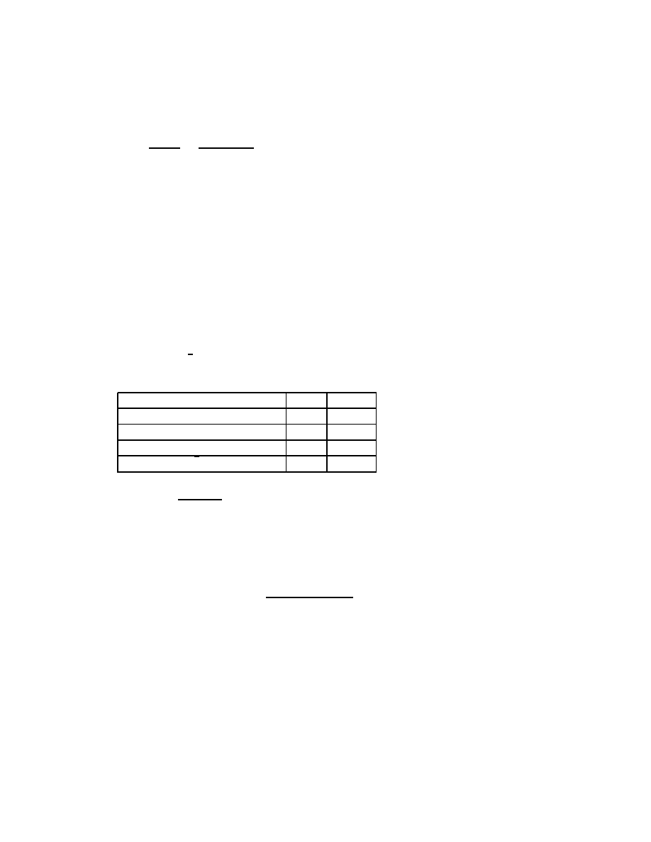
Example
5. Consider the equation y
′
=
3 − y
2
. We know the following:
• If y = 3, then y
′
= 0, flat slope,
• If y > 3, then y
′
< 0, down slope,
• If y < 3, then y
′
> 0, up slope.
See the directional field below (with some solutions sketched):
0
1
2
3
4
5
6
0
0.5
1
1.5
2
2.5
3
3.5
4
4.5
5
As t → ∞, we have y → 3.
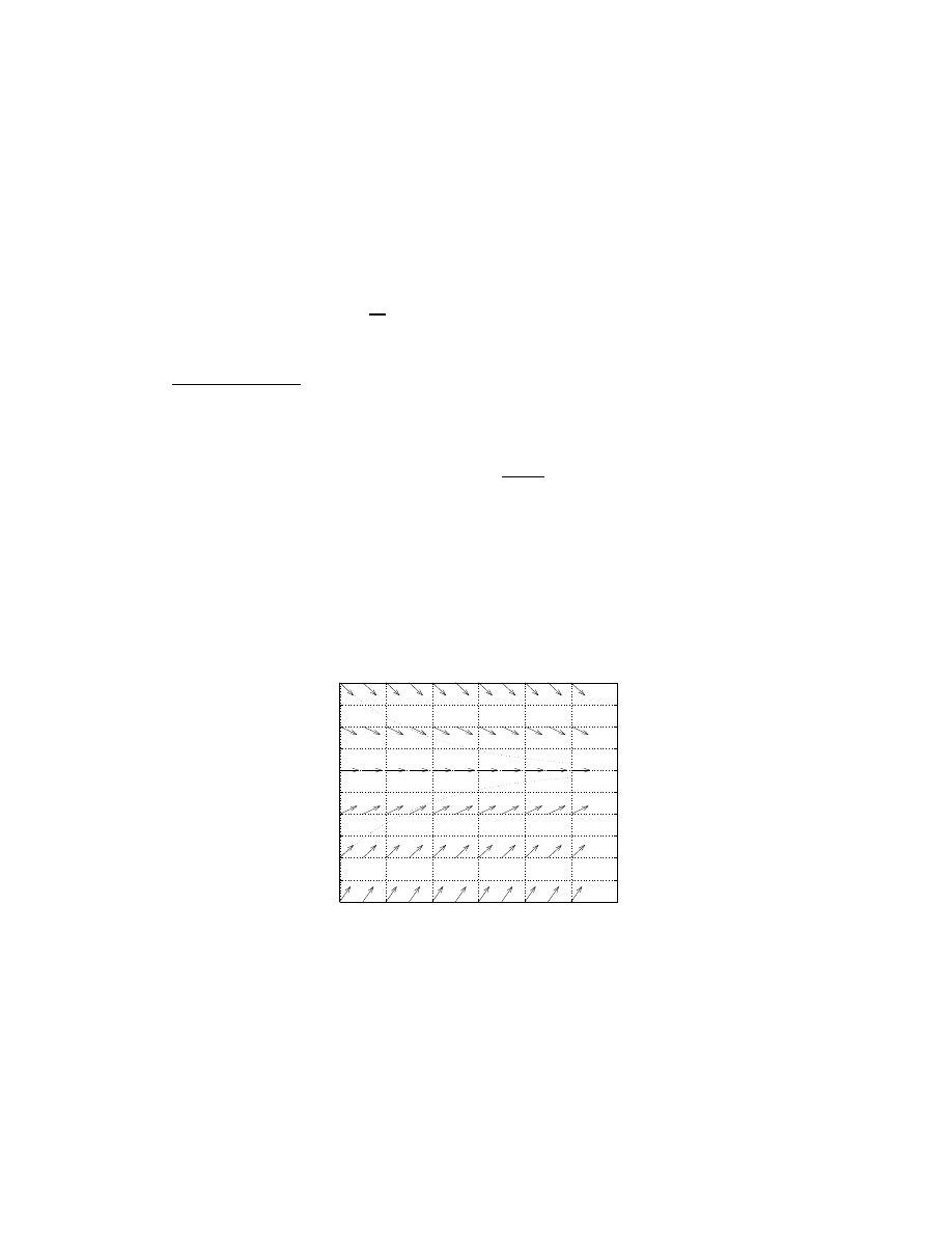
Example
6. y
′
= t + y
• We have y
′
= 0 when y = −t,
4
• We have y
′
> 0 when y > −t,
• We have y
′
< 0 when y < −t.
−1
0
1
2
3
4
5
−5
−4
−3
−2
−1
0
1
2
What can we say about the solutions?
This depends on the initial condition y(0) = y
0
.
• If y(0) > −1, then y → ∞ as t → ±∞.
• If y(0) < −1, then y → ∓∞ as t → ±∞.
• If y(0) = −1, the y(t) = −t − 1.
5

Chapter 2: First order Differential Equations
We consider the equation
dy
dt
= f (t, y)
Overview:
• Two special types of equations: linear, and separable;
• Linear vs. nonlinear;
• modeling;
• autonomous equations.
2.1: Linear equations; Method of integrating
factors
The function f (t, y) is a linear function in y, i.e, we can write
f (t, y) = −p(t)y + g(t).
So we will study the equation
y
′
+ p(t)y = g(t).
(A)
We introduce the method of integrating factors (due to Leibniz): We multiply
equation (A) by a function µ(t) on both sides
µ(t)y
′
+ µ(t)p(t)y = µ(t)g(t)
The function µ is chosen such that the equation is integrable, meaning the
LHS (Left Hand Side) is the derivative of something. In particular, we re-
quire:
µ(t)y
′
+ µ(t)p(t)y = (µ(t)y)
′
,
⇒
µ(t)y
′
+ µ(t)p(t)y = µ(t)y
′
+ µ
′
(t)y
6

which requires
µ
′
(t) =
dµ
dt
= µ(t)p(t),
⇒
dµ
µ
= p(t) dt
Integrating both sides
ln µ(t) =
Z
p(t) dt
which gives a formula to compute µ
µ(t) = exp
Z
p(t) dy
.
Therefore, this µ is called the integrating factor. Putting back into equation
(A), we get
d
dt
(µ(t)y) = µ(t)g(t),
µ(t)y =
Z
µ(t)g(t) dt + c
which give the formula for the solution
y(t) =
1
µ(t)
Z
µ(t)g(t) dt + c
,
where µ(t) = exp
Z
p(t) dt
.
Example
1. Solve y
′
+ ay = b (a 6= 0).
Answer.
We have p(t) = a and g(t) = b. So
µ = exp(
Z
a dt) = e
at
so
y = e
−at
Z
e
at
b dt = e
−at
b
a
e
at
+ c
=
b
a
+ ce
−at
,
where c is an arbitrary constant.
Example
2. Solve y
′
+ y = e
2t
.
Answer.
We have p(t) = 1 and g(t) = e
2t
. So
µ(t) = exp(
Z
1 dt) = e
t
7

and
y(t) = e
−t
Z
e
t
e
2t
dt = e
t
Z
e
3t
dt = e
−t
1
3
e
3t
+ c
=
1
3
e
2t
+ ce
−t
.
Example
3. Solve
(1 + t
2
)y
′
+ 4ty = (1 + t
2
)
−2
,
y(0) = 1.
Answer.
First, let’s rewrite the equation into the normal form
y
′
+
4t
1 + t
2
y = (1 + t
2
)
−3
,
so
p(t) =
4t
1 + t
2
,
g(t) = (1 + t
2
)
−3
.
Then
µ(t) = exp
Z
p(t) dt
= exp
Z
4t
1 + t
2
dt
= exp(2 ln(1 + t
2
)) = exp(ln(1 + t
2
)
2
) = (1 + t
2
)
2
.
Then
y = (1+t
2
)
−2
Z
(1+t
2
)
2
(1+t
2
)
−3
dt = (1+t
2
)
−2
Z
(1+t
2
)
−1
dt =
arctan t + c
(1 + t
2
)
2
.
By the IC y(0) = 1:
y(0) =
0 + c
1
= c = 1,
⇒
y(t) =
arctan t + 1
(1 + t
2
)
2
.
Example
4. Solve ty
′
− y = t
2
e
−t
, (t > 0).
Answer.
Rewrite it into normal form
y
′
−
1
t
y = te
−t
so
p(t) = −1/t,
g(t) = te
−t
.
8

We have
µ(t) = exp(
Z
(−1/t)dt) = exp(− ln t) =
1
t
and
y(t) = t
Z
1
t
te
−t
dt = t
Z
e
−t
dt = t(−e
−t
+ c) = −te
−t
+ ct.
Example
5. Solve y −
1
3
y = e
−t
, with y(0) = a, and discussion how the
behavior of y as t → ∞ depends on the initial value a.
Answer.
Let’s solve it first. We have
µ = e
−
1
3
t
so
y = e
1
3
t
Z
e
−
1
3
t
e
−t
dt = e
1
3
t
Z
e
−
4
3
t
dt = e
1
3
t
(−
3
4
e
−
4
3
t
+ c).
Plug in the IC to find c
y(0) = e
0
(−
3
4
+ c) = a,
c = a +
3
4
so
y(t) = e
1
3
t
−
3
4
e
−
4
3
t
+ a +
3
4
= −
3
4
e
−t
+ (a +
3
4
)e
t/3
.
To see the behavior of the solution, we see that it contains two terms. The
first term e
−t
goes to 0 as t grows. The second term e
t/3
goes to ∞ as t
grows, but the constant a +
3
4
is multiplied on it. So we have
• If a +
3
4
= 0, i.e., if a = −
3
4
, we have y → 0 as t → ∞;
• If a +
3
4
> 0, i.e., if a > −
3
4
, we have y → ∞ as t → ∞;
• If a +
3
4
< 0, i.e., if a < −
3
4
, we have y → −∞ as t → ∞;
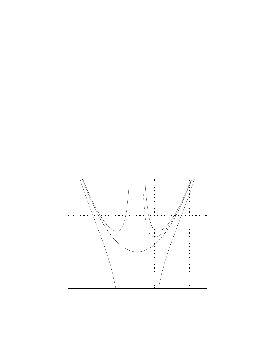
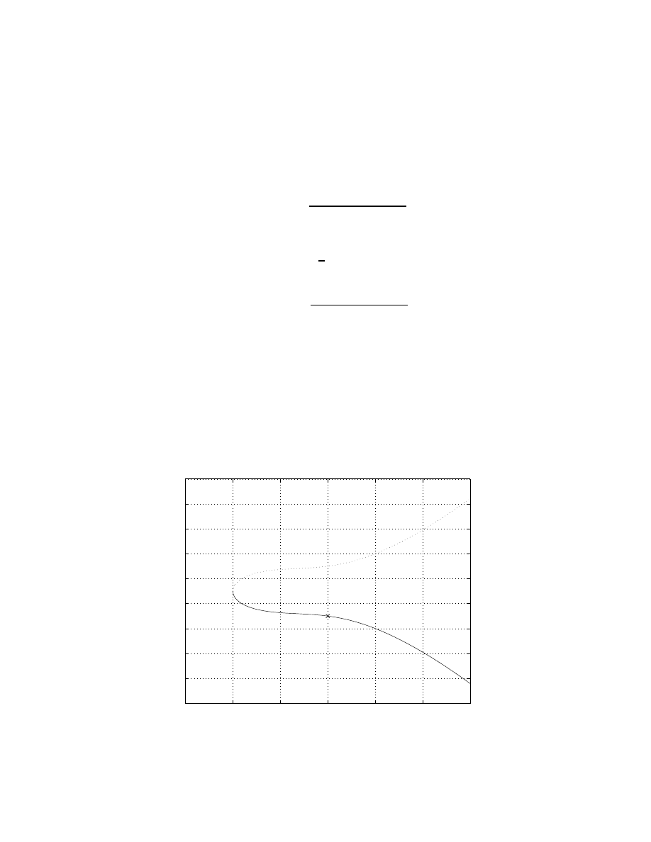
Example
6. Solve ty
′
+ 2y = 4t
2
, y(1) = 2.
Answer.
Rewrite the equation first
y
′
+
2
t
y = 4t,
(t 6= 0)
9
So p(t) = 2/t and g(t) = 4t. We have
µ(t) = exp(
Z
2/t dt) = exp(2 ln t) = t
2
and
y(t) = t
−2
Z
4t · t
2
dy = t
−2
(t
4
+ c)
By IC y(1) = 2,
y(1) = 1 + c = 2,
c = 1
we get the solution:
y(t) = t
2
+
1
t
2
,
t > 0.
Note the condition t > 0 comes from the fact that the initial condition is
given at t = 1, and we require t 6= 0.
In the graph below we plot several solutions in the t − y plan, depending on
initial data. The one for our solution is plotted with dashed line where the
initial point is marked with a ‘x’.
−4
−3
−2
−1
0
1
2
3
4
−5
0
5
10
10

2.2: Separable Equations
We study first order equations that can be written as
dy
dx
= f (x, y) =
M(x)
N(y)
where M(x) and N(y) are suitable functions of x and y only. Then we have
N(y) dy = M(x) dx,
⇒
Z
N(y) dy =
Z
M(x) dx
and we get implicitly defined solutions of y(x).
Example
1. Consider
dy
dx
=
sin x
1 − y
2
.
We can separate the variables:
Z
(1 − y
2
) dy =
Z
sin x dx,
⇒
y −
1
3
y
3
= − cos x + c.
If one has IC as y(π) = 2, then
2 −
1
3
· 2
3
= − cos π + c,
⇒
c = −
5
3
,
so the solution y(x) is implicitly given as
y −
1
3
y
3
+ cos x +
5
3
= 0.
Example
2. Find the solution in explicit form for the equation
dy
dx
=
3x
2
+ 4x + 2
2(y + 1)
,
y(0) = −1.
Answer.
Separate the variables
Z
2(y − 1) dy =
Z
(3x
2
+ 4x + 2) dx ,
⇒
(y − 1)
2
= x
3
+ 2x
2
+ 2x + c
11
Set in the IC y(0) = −1, i.e., y = −1 when x = 0, we get
(−1 − 1)
2
= 0 + c,
c = 4,
(y − 1)
2
= x
3
+ 2x
2
+ 2x + 4.
In explicitly form, one has two choices:
y(t) = 1 ±
√
x
3
+ 2x
2
+ 2x + 4.
To determine which sign is the correct one, we check again by the initial
condition:
y(0) = 1 ±
√
4 = 1 ± 2 = −1
We see we must choose the ‘-’ sign. The solution in explicitly form is:
y(x) = 1 −
√
x
3
+ 2x
2
+ 2x + 4.
On which interval will this solution be defined?
x
3
+ 2x
2
+ 2x + 4 ≥ 0, ⇒
x
2
(x + 2) + 2(x + 2) ≥ 0
⇒
(x
2
+ 2)(x + 2) ≥ 0, ⇒
x ≥ −2.
We can also argue that when x = −2, we have y = 1. At this point |dy/dx| →
∞, therefore solution can not be defined at this point.
The plot of the solution is given below, where the initial data is marked with
‘x’. We also include the solution with the ‘+’ sign, using dotted line.
−3
−2
−1
0
1
2
3
−8
−6
−4
−2
0
2
4
6
8
10
12

Example
3. Solve y
′
= 3x
2
+ 3x
2
y
2
, y(0) = 0, and find the interval where
the solution is defined.
Answer.
Let’s first separate the variables.
dy
dx
= 3x
2
(1 + y
2
),
⇒
Z
1
1 + y
2
dy =
Z
3x
2
dx,
⇒
arctan y = x
3
+ c.
Set in the IC:
arctan 0 = 0 + c,
⇒
c = 0
we get the solution
arctan y = x
3
,
⇒
y = tan(x
3
).
Since the initial data is given at x = 0, i.e., x
3
= 0, and tan is defined on the
interval (−
π
2
,
π
2
), we have
−
π
2
< x
3
<
π
2
,
⇒
−
h
π
2
i
1/3
< x <
h
π
2
i
1/3
.
Example
4. Solve
y
′
=
1 + 3x
2
3y
2
− 6y
,
y(0) = 1
and identify the interval where solution is valid.
Answer.
Separate the variables
Z
(3y
2
− 6y)dy =
Z
(1 + 3x
2
)dx y
3
− 3y
2
= x + x
3
+ c.
Set in the IC: x = 0, y = 1, we get
1 − 3 = c, ⇒
c = −2,
Then,
y
3
− 3y
2
= x
3
− x − 2.
Note that solution is given in implicitly form.
To find the valid interval of this solution, we note that y
′
is not defined is
3y
2
− 6y = 0, i.e., when y = 0 or y = 2. These are the two so-called “bad
13
points” where you can not define the solution. To find the corresponding
values of x, we use the solution expression:
y = 0 :
x
3
+ x − 2 = 0,
⇒
(x
2
+ x + 2)(x − 1) = 0, ⇒
x = 1
and
y = 2 :
x
3
+ x − 2 = −4, ⇒
x
3
+ x + 2 = 0,
⇒
(x
2
− x + 2)(x + 1) = 0, ⇒
x = −1
(Note that we used the facts x
2
+ x + 2 6= 0 and x
2
− x + 2 6= 0 for all x.)
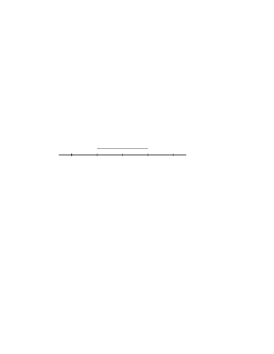
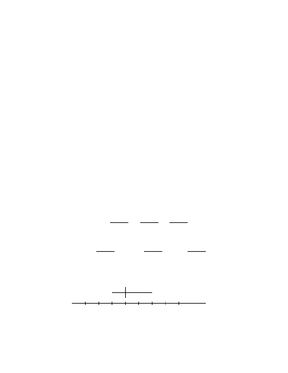
Draw the real line and work on it as following:
-
x
0
−1
−2
1
2
×
×
-
Therefore the interval is −1 < x < 1.
14

2.4: Differences between linear and nonlinear
equations
We will take this chapter before the modeling (ch. 2.3).
For a linear equation
y
′
+ p(t)y = g(t),
y(t
0
) = y
0
,
we have the following existence and uniqueness theorem.
Theorem
. If p(t) and g(t) are continuous and bounded on an open interval
containing t
0
, then it has an unique solution on that interval.
Example
1. Find the largest interval where the solution can be defined for
the following problems.
(A). ty
′
+ y = t
3
, y(−1) = 3.
Answer.
Rewrite: y
′
+
1
t
y = t
2
, so t 6= 0. Since t
0
= −1, the interval is
t < 0.
(B). ty
′
+ y = t
3
, y(1) = −3.
Answer.
The equation is same as (A), so t 6= 0. t
0
= 1, the interval is t > 0.
(C). (t − 3)y
′
+ (ln t)y = 2t, y(1) = 2
Answer.
Rewrite: y
′
+
ln t
t−3
y =
2t
t−3
, so t 6= 3 and t > 0 for the ln function.
Since t
0
= 1, the interval is then 0 < t < 3.
(D). y
′
+ (tan t)y = sin t, y(π) = 100.
Answer.
Since t
0
= π, and for tan t to be defined we must have t 6=
2k+1
2
π,
k = ±1, ±2, · · · . So the interval is
π
2
< t <
3π
2
.
For non-linear equation
y
′
= f (t, y),
y(t
0
) = y
0
,
we have the following theorem:
Theorem
. If f (t, y),
∂f
∂y
(t, y) are continuous and bounded on an rectangle
(α < t < β, a < y < b) containing (t
0
, y
0
), then there exists an open interval
around t
0
, contained in (α, β), where the solution exists and is unique.
15

We note that the statement of this theorem is not as strong as the one for
linear equation.
Below we give two counter examples.
Example
1. Loss of uniqueness. Consider
dy
dy
= f (t, y) = −
t
y
,
y(−2) = 0.
We first note that at y = 0, which is the initial value of y, we have y
′
=
f (t, y) → ∞. So the conditions of the Theorem are not satisfied, and we
expect something to go wrong.
Solve the equation as an separable equation, we get
Z
y dy = −
Z
t dt,
y
2
+ t
2
= c,
and by IC we get c = (−2)
2
+ 0 = 4, so y
2
+ t
2
= 4, and y = ±
√
4 − t
2
. Both
are solutions. We lose uniqueness of solutions.
Example
2. Blow-up of solution. Consider a simple non-linear equation:
y
′
= y
2
,
y(0) = 1.
Note that f (t, y) = y
2
, which is defined for all t and y. But, due to the
non-linearity of f , solution can not be defined for all t.
This equation can be easily solved as a separable equation.
Z
1
y
2
dy =
Z
dt,
−
1
y
= t + c,
y(t) =
−1
t + c
.
By IC y(0) = 1, we get 1 = −1/(0 + c), and so c = −1, and
y(t) =
−1
t − 1
.
We see that the solution blows up as t → 1, and can not be defined beyond
that point.
This kind of blow-up phenomenon is well-known for nonlinear equations.
16

2.3: Modeling with first order equations
General modeling concept: derivatives describe “rates of change”.
Model I: Exponential growth/decay.
Q(t) = amount of quantity at time t
Assume the rate of change of Q(t) is proportional to the quantity at time t.
We can write
dQ
dt
(t) = r · Q(t),
r : rate of growth/decay
If r > 0: exponential growth
If r < 0: exponential decay
Differential equation:
Q
′
= rQ,
Q(0) = Q
0
.
Solve it: separable equation.
Z
1
Q
dQ =
Z
r dt,
⇒
ln Q = rt + c,
⇒
Q(t) = e
rt+c
= ce
rt
Here r is called the growth rate. By IC, we get Q(0) = C = Q
0
. The solution
is
Q(t) = Q
0
e
rt
.
Two concepts:
• Doubling time T
D
(only if r > 0): is the time that Q(T
D
) = 2Q
0
.
Q(T
D
) = Q
0
e
rT
D
= 2Q
0
,
e
rT
D
= 2,
rT
D
= ln 2,
T
D
=
ln 2
r
.
• Half life (or half time) T
H
(only for r < 0): is the time that Q(T
H
) =
1
2
Q
0
.
Q(T
H
) = Q
0
e
rT
H
=
1
2
Q
0
,
e
rT
D
=
1
2
,
rT
D
= ln
1
2
= − ln 2, T
D
=
ln 2
−r
.
Note here that T
H
> 0 since r < 0.
17

NB! T
D
, T
H
do not depend on Q
0
. They only depend on r.
Example
1. If interest rate is 8%, compounded continuously, find doubling
time.
Answer.
Since r = 0.08, we have T
D
=
ln 2
0.08
.
Example
2. A radio active material is reduced to 1/3 after 10 years. Find
its half life.
Answer.
Model:
dQ
dt
= rQ, r is rate which is unknown. We have the solution
Q(t) = Q
0
e
rt
. So
Q(10) =
1
3
Q
0
,
Q
0
e
10r
=
1
3
Q
0
,
r =
− ln 3
10
.
To find the half life, we only need the rate r
T
H
= −
ln 2
r
= − ln 2
10
− ln 3
= 10
ln 2
ln 3
.
Model II: Interest rate/mortgage problems.
Example
3. Start an IRA account at age 25. Suppose deposit $2000 at the
beginning and $2000 each year after. Interest rate 8% annually, but assume
compounded continuously. Find total amount after 40 years.
Answer.
Set up the model: Let S(t) be the amount of money after t years
ds
dt
= 0.08S + 2000,
S(0) = 2000.
This is a first order linear equation. Solve it by integrating factor
S
′
− 0.08S = 2000,
µ = e
−0.08t
S(t) = e
0.08t
Z
2000 · e
−0.08t
dt = e
0.08t
2000
e
−0.08t
−0.08
+ c
=
2000
−0.08
+ ce
0.08t
By IC,
S(0) =
2000
−0.08
+ c = 2000,
C = 2000(1 +
1
0.08
) = 27000,
18

we get
S(t) = 27000e
0.08t
− 25000.
When t = 40, we have
S(40) = 27000 · e
3.2
− 25000 ≈ 637, 378.
Compare this to the total amount invested: 2000 + 2000 ∗ 40 = 82, 000.
Example
4: A home-buyer can pay $800 per month on mortgage payment.
Interest rate is 9% annually, (but compounded continuously), mortgage term
is 20 years. Determine maximum amount this buyer can afford to borrow.
Answer.
Set up the model: Let Q(t) be the amount borrowed (principle)
after t years
dQ
dt
= 0.09Q(t) − 800 ∗ 12
The terminal condition is given Q(20) = 0. We must find Q(0).
Solve the differential equation:
Q
′
− 0.09Q = −9600,
µ = e
−0.09t
Q(t) = e
0.09t
Z
(−9600)e
−0.09t
dt = e
0.09t
−9600
e
−0.09t
−0.09
+ c
=
9600
0.09
+ ce
0.09t
By terminal condition
Q(20) =
9600
0.09
+ ce
0.09∗20
= 0,
c = −
9600
0.09 · e
1.8
so we get
Q(t) =
9600
0.09
−
9600
0.09 · e
1.8
e
0.09t
.
Now we can get the initial amount
Q(0) =
9600
0.09
−
9600
0.09 · e
1.8
=
9600
0.09
(1 − e
−1.8
) ≈ 89, 034.79.
Model III: Mixing Problem.
Example
5. At t = 0, a tank contains Q
0
lb of salt dissolved in 100 gal of
water. Assume that water containing 1/4 lb of salt per gal is entering the
tank at a rate of r gal/min. At the same time, the well-mixed mixture is
draining from the tank at the same rate.
19

(1). Find the amount of salt in the tank at any time t ≥ 0.
(2). When t → ∞, meaning after a long time, what is the limit amount
Q
L
?
Answer.
Set up the model:
Q(t) = amount (lb) of salt in the tank at time t (min)
In-rate: r gal/min × 1/4 lb/gal =
r
4
lb/min
Out-rate: r gal/min × Q(t)/100 lb/gal =
Q
100
r lb/min
dQ
dt
= [In-rate] − [Out-rate] =
r
4
−
r
100
Q,
IC. Q(0) = Q
0
.
(1). Solve the equation
Q
′
+
r
100
Q =
r
4
,
µ = e
(r/100)t
.
Q(t) = e
−(r/100)t
Z
r
4
e
(r/100)t
dt = e
−(r/100)t
r
4
e
(r/100)t
100
r
+ c
= 25+ce
−(r/100)t
.
By IC
Q(0) = 25 + c = Q
0
,
c = Q
0
− 25,
we get
Q(t) = 25 + (Q
0
− 25)e
−(r/100)t
.
(2). As t → ∞, the exponential term goes to 0, and we have
Q
L
= lim
t→∞
Q(t) = 25lb.
Example
6. Tank contains 50 lb of salt dissolved in 100 gal of water. Tank
capacity is 400 gal. From t = 0, 1/4 lb of salt/gal is entering at a rate of 4
gal/min, and the well-mixed mixture is drained at 2 gal/min. Find:
(1) time t when it overflows;
(2) amount of salt before overflow;
(3) the concentration of salt at overflow.
20

Answer.
(1). Since the inflow rate 4 gal/min is larger than the outflow rate
2 gal/min, the tank will be filled up at t
f
:
t
f
=
400 − 100
4 − 2
= 150min.
(2). Let Q(t) be the amount of salt at t min.
In-rate: 1/4 lb/gal × 4 gal/min = 1 lb/min
Out-rate: 2 gal/min ×
Q(t)
100+2t
lb/gal =
Q
50+t
lb/min
dQ
dt
= 1 −
Q
50 + t
,
Q
′
+
1
50 + t
Q = 1,
Q(0) = 50
µ = exp(
Z
1
50 + t
dt) = exp(ln(50 + t)) = 50 + t
Q(t) =
1
50 + t
Z
(50 + t)dt =
1
50 + t
[50t +
1
2
t
2
+ c]
By IC:
Q(0) = c/50 = 50,
c = 2500,
We get
Q(t) =
50t + t
2
/2 + 2500
50 + t
.
(3). The concentration of salt at overflow time t = 150 is
Q(150)
400
=
50 · 150 + 150
2
/2 + 2500
400(50 + 150)
=
17
64
lb/gal.
Model IV: Air resistance
Example
7. A ball with mass 0.5 kg is thrown upward with initial velocity
10 m/sec from the roof of a building 30 meter high. Assume air resistance is
|v|/20. Find the max height above ground the ball reaches.
Answer.
Let S(t) be the position (m) of the ball at time t sec. Then, the
velocity is v(t) = dS/dt, and the acceleration is a = dv/dt. Let upward be
the positive direction. We have by Newton’s Law:
F = ma = −mg −
v
20
,
a = −g −
v
20m
=
dv
dt
21

Here g = 9.8 is the gravity, and m = 0.5 is the mass. We have an equation
for v:
dv
dt
= −
1
10
v − 9.8 = −0.1(v + 98),
so
Z
1
v + 98
dv =
Z
(−0.1)dt, ⇒
ln |v + 98| = −0.1t + c
which gives
v + 98 = ¯
ce
−0.1t
,
⇒
v = −98 + ¯ce
−0.1t
.
By IC:
v(0) = −98 + ¯c = 10,
¯
c = 108,
⇒
v = −98 + 108e
−0.1t
.
To find the position S, we use S
′
= v and integrate
S(t) =
Z
v(t) dt =
Z
(−98 + 108e
−0.1t
)dt = −98t + 108e
−0.1t
/(−0.1) + c
By IC for S,
S(0) = −1080 + c = 30,
c = 1110,
S(t) = −98t − 1080e
−0.1t
+ 1110.
At the maximum height, we have v = 0. Let’s find out the time T when max
height is reached.
v(T ) = 0,
−98 + 108e
−0.1T
= 0,
98 = 108e
−0.1T
,
e
−0.1T
= 98/108,
−0.1T = ln(98/108), T = −10 ln(98/108) = ln(108/98).
So the max height S
M
is
S
M
= S(T ) = − 980 ln
108
98
− 1080e
−0.1 ln(108/98)
+ 1110
= −980 ln
108
98
− 1080(98/108) + 1110 ≈ 34.78 m.
Other possible questions:
• Find the time when the ball hit the ground.
Solution: Find the time t = t
H
for S(t
H
) = 0.
22

• Find the speed when the ball hit the ground.
Solution: Compute |v(t
H
)|.
• Find the total distance traveled by the ball when it hits the ground.
Solution: Add up twice the max height S
M
with the height of the
building.
23
2.5: Autonomous equations and population dy-
namics
Definition: An autonomous equation is of the form y
′
= f (y), where the
function f for the derivative depends only on y, not on t.
Simplest example: y
′
= ry, exponential growth/decay, where solution is
y = y
0
e
rt
.
Definition: Zeros of f where f (y) = 0 are called critical points or equilibrium
points, or equilibrium solutions.
Why? Because if f (y
0
) = 0, then y(t) = y
0
is a constant solution. It is called
an equilibrium.
Question: Is an equilibrium stable or unstable?
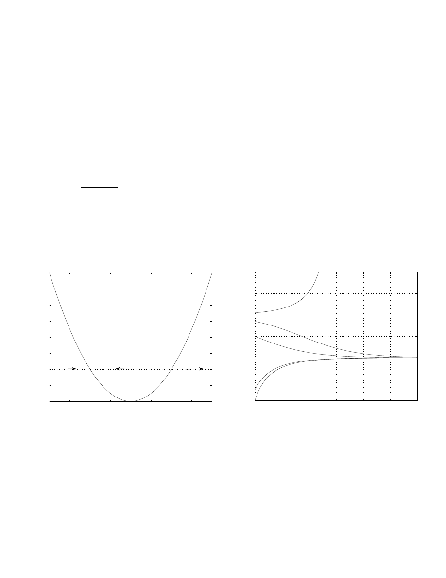
Example
1. y
′
= y(y − 2). We have two critical points: y
1
= 0, y
2
= 2.
−1
−0.5
0
0.5
1
1.5
2
2.5
3
−1
−0.5
0
0.5
1
1.5
2
2.5
3
y
f
+
+
_
0
0.5
1
1.5
2
2.5
3
−2
−1
0
1
2
3
4
t
y
We see that y
1
= 0 is stable, and y
2
= 2 is unstable.
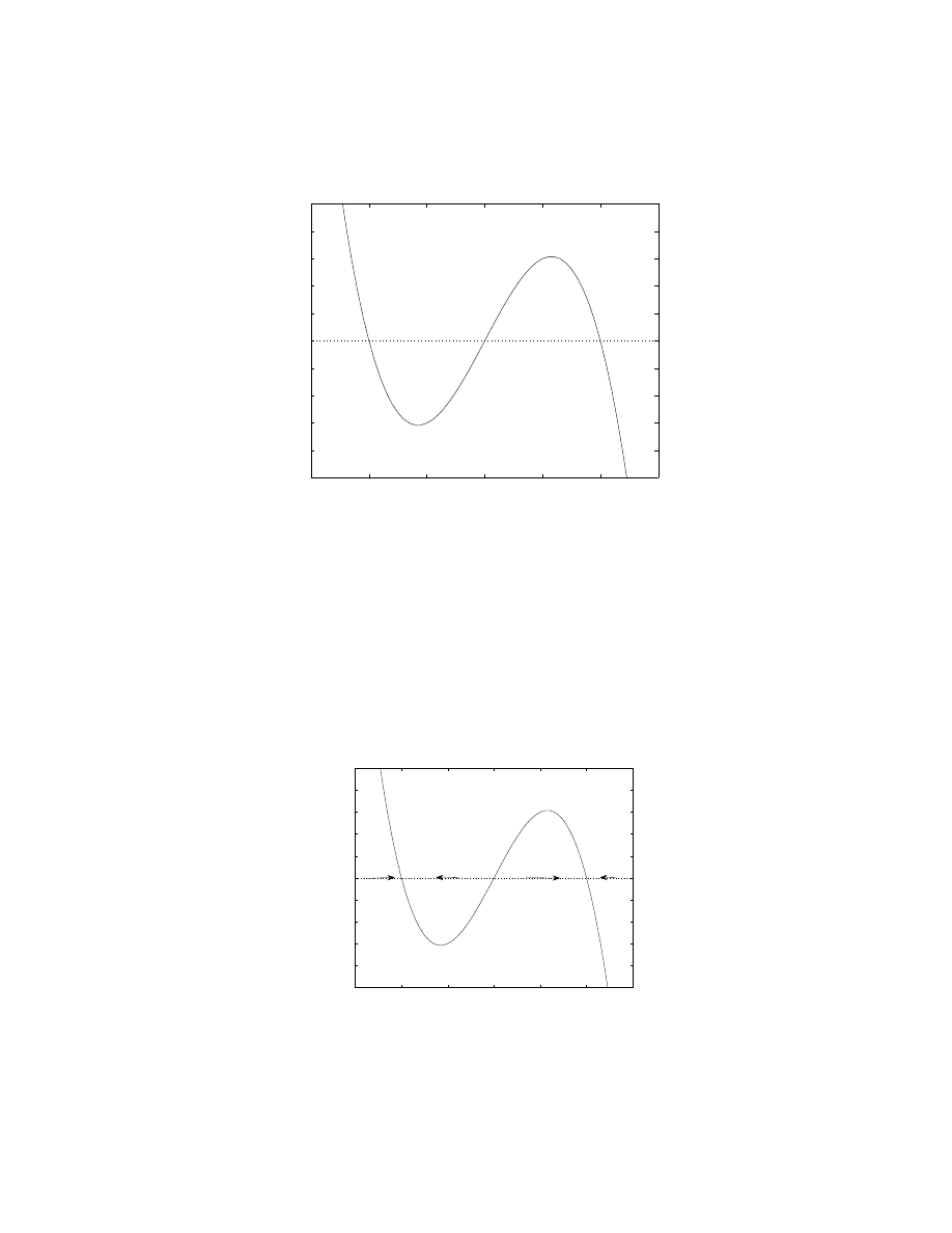
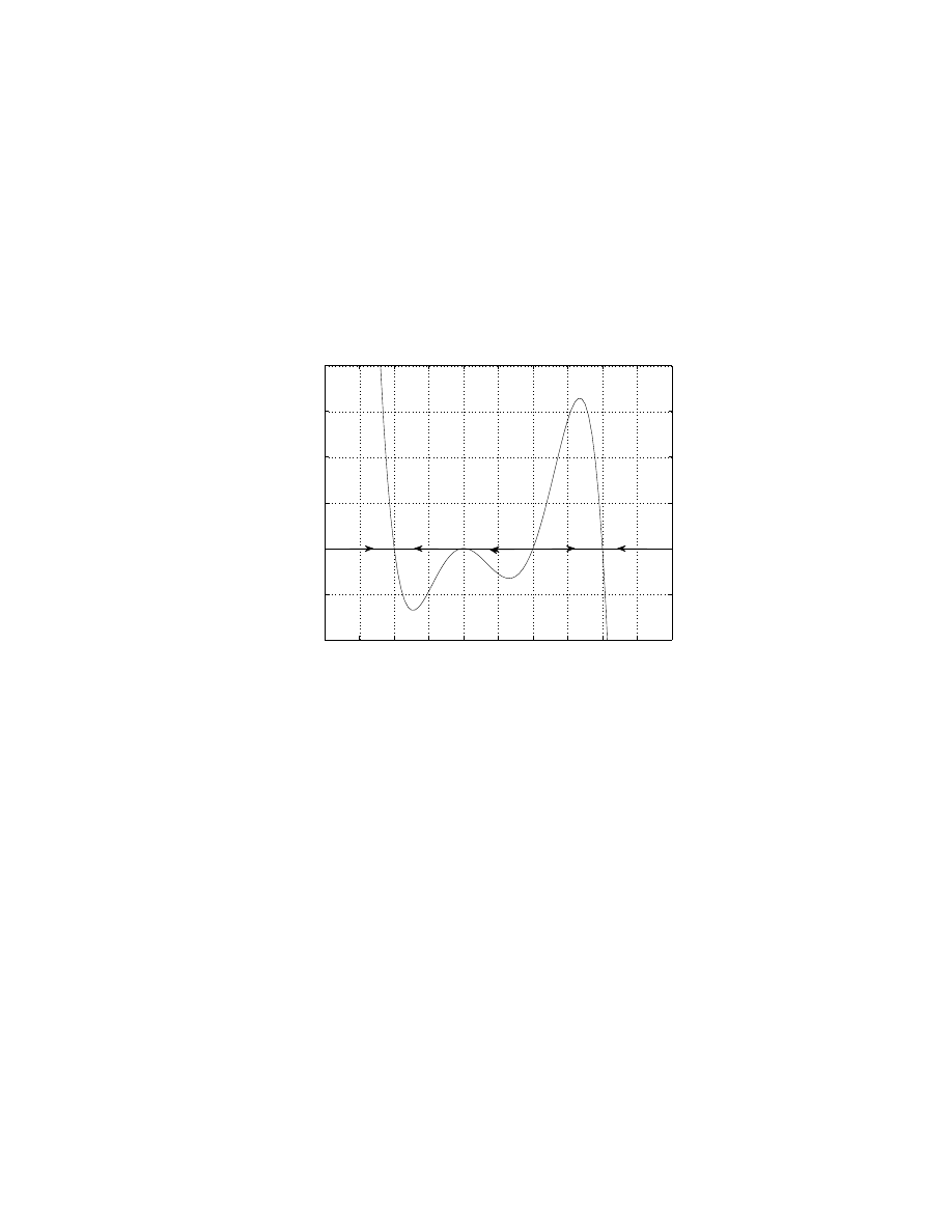
Example
2. For the equation y
′
= f (y) where f (y) is given in the following
plot:
24
0
1
2
3
4
5
6
−5
−4
−3
−2
−1
0
1
2
3
4
5
y
f
• (A). What are the critical points?
• (B). Are they stable or unstable?
• (C) Sketch the solutions in the t − y plan, and describe the behavior of
y as t → ∞ (as it depends on the initial value y(0).)
Answer.
(A). There are three critical points: y
1
= 1, y
2
= 3, y
3
= 5.
(B). To see the stability, we add arrows on the y-axis:
0
1
2
3
4
5
6
−5
−4
−3
−2
−1
0
1
2
3
4
5
y
f
+
_
+
_
We see that y
1
= 1 is stable, y
2
= 3 is unstable, and y
3
= 5 is stable.
25
(C). The sketch is given below:
0
0.1
0.2
0.3
0.4
0.5
0.6
0.7
0.8
0.9
1
0
1
2
3
4
5
6
t
y
Asymptotic behavior for y as t → ∞ depends on the initial value of y:
• If y(0) < 1, then y(t) → 1,
• If y(0) = 1, then y(t) = 1;
• If 1 < y(0) < 3, then y(t) → 1;
• If y(0) = 3, then y(t) = 3;
• If 3 < y(0) < 5, then y(t) → 5;
• If y(0) = 5, then y(t) = 5;
• if y(t) > 5, then y(t) → 5.
Stability: is not only stable or unstable.
Example
3. For y
′
= y
2
, we have only one critical point y
1
= 0. For y < 0,
we have y
′
> 0, and for y > 0 we also have y
′
> 0. So solution is increasing
26
on both intervals. So on the interval y < 0, solution approaches y = 0 as t
grows, so it is stable. But on the interval y > 0, solution grows and leaves
y = 0, and it is unstable. This type of critical point is called semi-stable.
This happens when one has a double root for f (y) = 0.
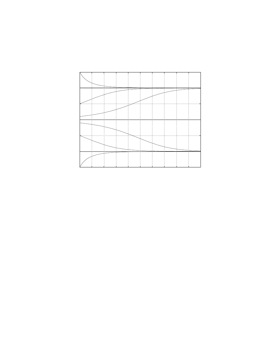
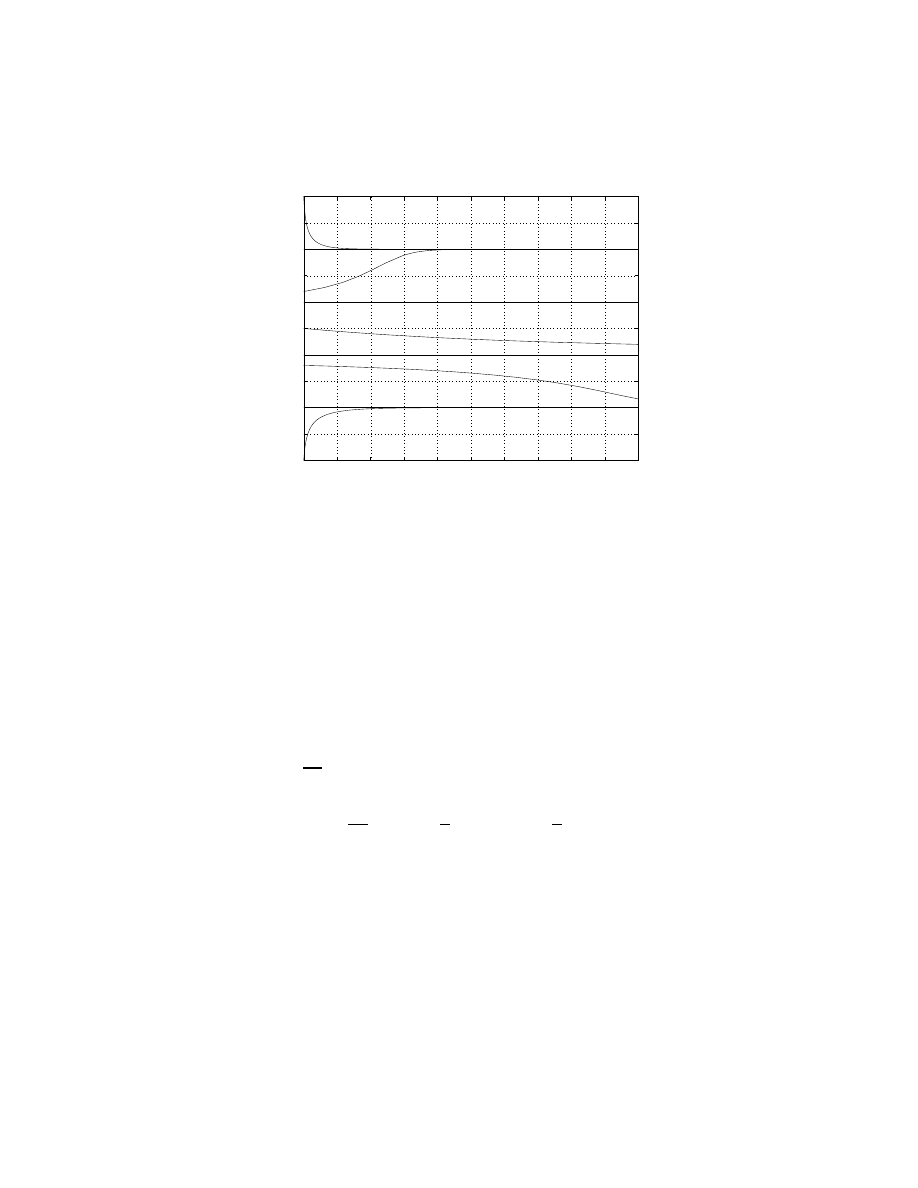
Example
4. For equation y
′
= f (y) where f (y) is given in the plot
−1
−0.5
0
0.5
1
1.5
2
2.5
3
3.5
4
−1
−0.5
0
0.5
1
1.5
2
y
f
• (A). Identify equilibrium points;
• (B). Discuss their stabilities;
• (C). Sketch solution in y − t plan;
• (D). Discuss asymptotic behavior as t → ∞.
Answer.
(A). y = 0, y = 1, y = 2, y = 3 are the critical points.
(B). y = 0 is stable, y = 1 is semi-stable, y = 2 is unstable, and y = 3 is
stable.
(C). The Sketch is given in the plot:
27
0
0.2
0.4
0.6
0.8
1
1.2
1.4
1.6
1.8
2
−1
−0.5
0
0.5
1
1.5
2
2.5
3
3.5
4
t
y
(D). The asymptotic behavior as t → ∞ depends on the initial data.
• If y(0) < 1, then y → 0;
• If 1 ≤ y(0) < 2, then y → 1;
• If y(0) = 2, then y(t) = 2;
• If y(0) > 2, then y → 3.
Application in population dynamics: let y(t) be the population of a species.
dy
dt
= (r − ay)y.
the logistic equation
dy
dt
= r(1 −
y
k
))y,
k =
r
a
,
r=intrinsic growth rate,
k=environmental carrying capacity.
critical points: y = 0, y = k. Here y = 0 is unstable, and y = k is stable.
If 0 < y(0) < k, then y → k as t grows.
28

Chapter 3: Second Order Linear Equations
General form of the equation:
a
2
(t)y
′′
+ a
1
(t)y
′
+ a
0
(t)y = b(t),
where
a
2
(t) 6= 0,
y(t
0
) = y
0
, y
′
(t
0
) = ¯
y
0
.
If b(t) ≡ 0, we call it homogeneous. Otherwise, it is called non-homogeneous.
3.1: Homogeneous equations with constant co-
efficients
This is the simplest case: a
2
, a
1
, a
0
are all constants, and g = 0. Let’s write:
a
2
y
′′
+ a
1
y
′
+ a
0
= 0.
Example
1. Solve y
′′
= y = 0, (we have here a
2
= 1, a
1
= 0, a
0
= 1).
Answer.
Guess y
1
(t) = e
t
.
Check: y
′′
= e
t
, so y
′′
− y = e
t
− e
t
= 0, ok.
Guess another: y
2
(t) = e
−t
.
Check: y
′
= −e
−t
, so y
′′
= e
−t
, so y
′′
− y = e
t
− e
t
= 0, ok.
Observation: Another function y = c
1
y
1
+ c
2
y
2
for any arbitrary constant
c
1
, c
2
(this is called a “linear combination of y
1
, y
2
.) is also a solution.
Check:
y = c
1
e
t
+ c
2
e
−t
,
then
y
′
= c
1
e
t
− c
2
e
−t
,
y
′′
= c
1
e
t
+ c
2
e
−t
,
⇒
y
′′
− y = 0.
Actually this is a general property. It is called the principle of superposition.
Theorem
Let y
1
(t) and y
2
(t) be solutions of
a
2
(t)y
′′
+ a
1
(t)y
′
+ a
0
(t)y = 0
29

Then, y = c
1
y
1
+ c
2
y
2
for any constants c
1
, c
2
is also a solution.
Proof
: If y
1
solves the equation, then
a
2
(t)y
′′
1
+ a
1
(t)y
′
1
+ a
0
(t)y
1
= 0.
(I)
If y
2
solves the equation, then
a
2
(t)y
′′
2
+ a
1
(t)y
′
2
+ a
0
(t)y
2
= 0.
(II)
Multiple (I) by c
1
and (II) by c
2
, and add them up:
a
2
(t)(c
1
y
1
+ c
2
y
2
)
′′
+ a
1
(t)(c
1
y
1
+ c
2
y
2
)
′
+ a
0
(t)(c
1
y
1
+ c
2
y
2
) = 0.
Let y = c
1
y
1
+ c
2
y
2
, we have
a
2
(t)y
′′
+ a
1
(t)y
′
+ a
0
(t)y = 0
therefore y is also a solution to the equation.
How to find the solutions of a
2
y
′′
+ a
1
y
′
+ a
0
y = 0?
We seek solutions in the form y(t) = e
rt
. Find r.
y
′
= re
rt
= ry,
y
′′
= r
2
e
rt
= r
2
y
a
2
r
2
y + a
1
ry + a
0
y = 0
Since y 6= 0, we get
a
2
r
2
+ a
1
r
1
+ a
0
= 0
This is called the characteristic equation.
Conclusion: If r is a root of the characteristic equation, then y = e
rt
is a
solution.
If there are two real and distinct roots r
1
6= r
2
, then the general solution is
y(t) = c
1
e
r
1
t
+c
2
e
r
2
t
where c
1
, c
2
are two arbitrary constants to be determined
by initial conditions (ICs).
Example
2. Consider y
′′
− 5y
′
+ 6y = 0.
• (a). Find the general solution.
30

• (b). If ICs are given as: y(0) = −1, y
′
(0) = 5, find the solution.
• (c) What happens when t → ∞?
Answer.
(a). The characteristic equation is: r
2
−5r+6 =, so (r−2)(r−3) =
0, two roots: r
1
= 2, r
2
= 3. General solution is:
y(t) = c
1
e
2t
+ c
2
e
3t
.
(b). y(0) = −1 gives: c
1
+ c
2
= −1.
y
′
(0) = 5: we have y
′
= 2c
1
e
2t
+ 3c
2
e
3t
, so y
′
(0) = 2c
1
+ 3c
2
= 5.
Solve these two equations for c
1
, c
2
: Plug in c
2
= −1 − c
1
into the second
equation, we get 2c
1
+ 3(−1−c
1
) = 5, so c
1
= −8. Then c
2
= 7. The solution
is
y(t) = −8e
2t
+ 7e
3t
.
(c). We see that y(t) = e
2t
· (−8 + te
t
), and both terms in the product go to
infinity as t grows. So y → ∞.
Example
3. Find the solution for 2y
′′
+ y
′
− y = 0, with initial conditions
y(1) = 0, y
′
(1) = 3.
Answer.
Characteristic equation:
2r
2
+ r − 1 = 0, ⇒
(2r − 1)(r + 1) = 0, ⇒
r
1
=
1
2
, r
2
= −1.
General solution is:
y(t) = c
1
e
t
2
+ c
2
e
−t
.
The ICs give
y(1) = 0 :
c
1
e
1
2
+ c
2
e
−1
= 0.
(A)
y
′
(1) = 3 :
y
′
(t) =
1
2
c
1
e
1
2
t
− c
2
e
−t
,
1
2
c
1
e
1
2
− c
2
e
−1
= 3.
(B)
(A)+(B) gives
3
2
c
1
e
1
2
= 3,
c
1
= 2e
−
1
2
.
Plug this in (A):
c
2
= −ec
1
e
1
2
= −e2e
1
2
e
1
2
= −2e.
31

The solution is
y(t) = 2e
−
1
2
e
1
2
t − 2ee
−t
= 2e
1
2
(t−1)
− 2e
−t+1
,
and as t → ∞ we have y → ∞.
Summary of receipt:
1. Write the characteristic equation;
2. Find the roots;
3. Write the general solution;
4. Set in ICs to get the arbitrary constants c
1
, c
2
.
Example
4. Consider the equation y
′′
− 5y = 0.
• (a). Find the general solution.
• (b). If y(0) = 1, what should y
′
(0) be such that y remain bounded as
t → +∞?
Answer.
(a). Characteristic equation
r
2
− 5 = 0, ⇒
r
1
= −
√
5, r
2
=
√
5.
General solution is
y(t) = c
1
e
−
√
5t
+ c
2
e
√
5t
.
(b). If y(t) remains bounded as t → ∞, then the term e
√
5t
must vanish,
which means we must have c
2
= 0. This means y(t) = c
1
e
−
√
5t
. If y(0) = 1,
then y(0) = c
1
= 1, so y(t) = e
−
√
5t
. This gives y
′
(t) = −
√
5e
−
√
5t
which
means y
′
(0) = −
√
5.
Example
5. Consider the equation 2y
′′
+ 3y
′
= 0. The characteristic equa-
tion is
2r
2
+ 3r = 0,
⇒
r(2r + 3) = 0,
⇒
r
1
= −
3
2
, r
2
= 0
32

The general solutions is
y(t) = c
1
e
−
3
2
t
+ c
2
e
0t
= c
1
e
−
3
2
t
+ c
2
.
As t → ∞, the first term in y vanished, and we have y → c
2
.
Example
6. Find a 2nd order equation such that c
1
e
3t
+ c
2
e
−t
is its general
solution.
Answer.
From the form of the general solution, we see the two roots are
r
1
= 3, r
2
= −1. The characteristic equation could be (r − 3)(r + 1) = 0, or
this equation multiplied by any non-zero constant. So r
2
− 2r − 3 = 0, which
gives us the equation
y
′′
− 2y
′
− 3y = 0.
NB! This answer is not unique. Multiple it by any non-zero constant gives
another equation.
33
3.2: Solutions of Linear Homogeneous Equa-
tions; the Wronskian
We consider some theoretical aspects of the solutions to a general 2nd order
linear equations.
Theorem
. (Existence and Uniqueness Theorem) Consider the initial value
problem
y
′′
+ p(t)y
′
+ q(t)y = g(t),
y(t
0
) = y
0
,
y
′
(t
0
) = ¯
y
0
.
If p(t), q(t) and g(t) are continuous and bounded on an open interval I con-
taining t
0
, then there exists exactly one solution y(t) of this equation, valid
on I.
Example
1. Given the equation
(t
2
− 3t)y
′′
+ ty
′
− (t + 3)y = e
t
,
y(1) = 2,
y
′
(1) = 1.
Find the largest interval where solution is valid.
Answer.
Rewrite the equation into the proper form:
y
′′
+
t
t(t − 3)
y
′
−
t + 3
t(t − 3)
y =
e
t
t(t − 3)
,
so we have
p(t) =
t
t(t − 3)
,
q(t) = −
t + 3
t(t − 3)
,
g(t) =
e
t
t(t − 3)
.
We see that we must have t 6= 0 and t 6= 3. Since t
0
= 1, then the largest
interval is I = (0, 3), or 0 < t < 3. See the figure below.
-
x
0
1
2
3
×
×
t
0
?
-
34

Definition
. Given two functions f (t), g(t), the Wronskian is defined as
W (f, g)(t) ˙
= f g
′
− f
′
g.
Remark: One way to remember this definition could be using the determi-
nant,
W (f, g)(t) =
f
g
f
′
g
′
.
Main property of the Wronskian:
• If W (f, g) ≡ 0, then f anf g are linearly dependent.
• Otherwise, they are linearly independent.
Example
2. Check if the given pair of functions are linearly dependent or
not.
(a). f = e
t
, g = e
−t
.
Answer.
We have
W (f, g) = e
t
(−e
−t
) − e
t
e
−t
= −2 6= 0
so they are linearly independent.
(b). f (t) = sin t, g(t) = cos t.
Answer.
We have
W (f, g) = sin t(sin t) − cos t cos t = −1 6= 0
and they are linearly independent.
(c). f (t) = t + 1, g(t) = 4t + 4.
Answer.
We have
W (f, g) = (t + 1)4 − (4t + 4) = 0
so they are linearly dependent. (In fact, we have g(t) = 4 · f(t).)
35

(d). f (t) = 2t, g(t) = |t|.
Answer.
Note that g
′
(t) = sign(t) where sign is the sign function. So
W (f, g) = 2t · sign(t) − 2|t| = 0
(we used t · sign(t) = |t|). So they are linearly dependent.
Theorem
. Suppose y
1
(t), y
2
(t) are two solutions of
y
′′
+ p(t)y
′
+ q(t)y = 0.
Then
(I) We have either W (y
1
, y
2
) ≡ 0 or W (y
1
, y
2
) never zero;
(II) If W (y
1
, y
2
) 6= 0, the y = c
1
y
1
+ c
2
y
2
is the general solution. They are
also called to form a fundamental set of solutions. As a consequence,
for any ICs y(t
0
) = y
0
, y
′
(t
0
) = ¯
y
0
, there is a unique set of (c
1
, c
2
) that
give a unique solution.
The next Theorem is probably the most important one in this chapter.
Theorem
(Abel’s Theorem) Let y
1
, y
2
be two (linearly independent) solutions
to y
′′
+ p(t)y
′
+ q(t)y = 0 on an open interval I. Then, the Wronskian
W (y
1
, y
2
) on I is given by
W (y
1
, y
2
)(t) = C · exp(
Z
−p(t) dt),
for some constant C depending on y
1
, y
2
, but independent on t in I.
Proof
. We skip this part. Read the book for a proof.
Example
3. Given
t
2
y
′′
− t(t + 2)y
′
+ (t + 2)y = 0.
36

Find W (y
1
, y
2
) without solving the equation.
Answer.
We first find the p(t)
p(t) = −
t + 2
t
which is valid for t 6= 0. By Abel’s Theorem, we have
W (y
1
, y
2
) = C · exp(
Z
−p(t) dt) = C · exp(
Z
t + 2
t
dt) = Ce
t+2 ln |t|
= Ct
2
e
t
.
NB! The solutions are defined on either (0, ∞) or (−∞, 0), depending on t
0
.
From now on, when we say two solutions y
1
, y
2
of the solution, we mean two
linearly independent solutions that can form a fundamental set of solutions.
Example
4. If y
1
, y
2
are two solutions of
ty
′′
+ 2y
′
+ te
t
y = 0,
and W (y
1
, y
2
)(1) = 2, find W (y
1
, y
2
)(5).
Answer.
First we find that p(t) = 2/t. By Abel’s Theorem we have
W (y
1
, y
2
)(t) = C · exp
−
Z
2
t
dt
= C · e
− ln t
= Ct
−2
.
If W (y
1
, y
2
)(1) = 2, then C1
−2
= 2, which gives C = 2. So we have
W (y
1
, y
2
)(5) = 25
−2
=
2
25
.
Example
5. If W (f, g) = 3e
4t
, and f = e
2t
, find g.
Answer.
By definition of the Wronskian, we have
W (f, g) = f g
′
− f
′
g = e
2t
g
′
− 2e
2t
g = 3e
4t
,
which gives a 1st order equation for g:
g
′
− 2g = 3e
2t
.
37

Solve it for g:
µ(t) = e
−2t
,
g(t) = e
2t
Z
e
−2t
3e
2t
dy = e
2t
(3t + c).
We can choose c = 0, and get g(t) = 3te
2t
.
Next example shows how Abel’s Theorem can be used to solve 2nd order
differential equations.
Example
6. Consider the equation y
′′
+ 2y
′
+ y = 0. Find the general
solution.
Answer.
The characteristic equation is r
2
+ 2r + 1 = 0, which given double
roots r
1
= r
2
= −1. So we know that y
1
= e
−t
is a solutions. How can we
find another solution y
2
that’s linearly independent?
By Abel’s Theorem, we have
W (y
1
, y
2
) = C exp
Z
−2 dt
= Ce
−2t
,
and we can choose C = 1 and get W (y
1
, y
2
) = e
−2t
. By the definition of the
Wronskian, we have
W (y
1
, y
2
) = y
1
y
′
2
− y
′
1
y
2
= e
−t
y
′
2
− (−e
−t
y
2
) = e
−t
(y
′
2
+ y
2
).
These two computation must have the same answer, so
e
−t
(y
′
2
+ y
2
) = e
−2t
,
y
′
2
+ y
2
= e
−t
.
This is a 1st order equation for y
2
. Solve it:
µ(t) = e
t
,
y
2
(t) = e
−t
Z
e
t
e
−t
dt = e
−t
(t + c).
Choosing c = 0, we get y
2
= te
t
. The general solution is
y(t) = c
1
y
1
+ c
2
y
2
= c
1
e
−t
+ c
2
te
−t
.
This is called the method of reduction of order. We will study it more later
in chapter 3.4.
38

3.3: Complex Roots
The roots of the characteristic equation can be complex numbers. Consider
the equation
ay
′′
+ by
′
+ cy = 0,
→
ar
2
+ br + c = 0.
The two roots are
r
1,2
=
−b ±
√
b
2
− 4ac
2a
.
If b
2
− 4ac < 0, the root are complex, i.e., a pair of complex conjugate
numbers. We will write r
1,2
= λ ± iµ. There are two solutions:
y
1
= e
(λ+iµ)t
= e
λt
e
iµt
,
y
2
= y
1
= e
(λ−iµ)t
= e
λt
e
−iµt
.
To deal with exponential function with pure imaginary exponent, we need
the Euler’s Formula:
e
iβ
= cos β + i sin β.
A couple of Examples to practice this formula:
e
i
5
6
π
= cos
5
6
π + i sin
5
6
π = −
√
3
2
+ i
1
2
.
e
iπ
= cos π + i sin π = −1.
e
a+ib
= e
a
e
ib
= e
a
(cos b + i sin b).
Back to y
1
, y
2
, we have
y
1
= e
λt
(cos µt + i sin µt),
y
2
= e
λt
(cos µt + i sin µt).
But these solutions are complex valued. We want real-valued solutions! To
achieve this, we use the Principle of Superposition. If y
1
, y
2
are two solutions,
then
1
2
(y
1
+ y
2
),
1
2i
(y
1
− y
2
) are also solutions. Let
˜
y
1
˙
=
1
2
(y
1
+ y
2
) = e
λt
cos µt,
˜
y
2
˙
=
1
2i
(y
1
− y
2
) = e
λt
sin µt.
To make sure they are linearly independent, we can check the Wronskian,
W (˜
y
1
, ˜
y
2
) = µe
2λt
6= 0. (home work problem).
39

So y
1
, y
2
are linearly independent, and we have the general solution
y(t) = c
1
e
λt
cos µt + c
2
e
λt
sin µt = e
λt
(c
1
cos µt + c
2
sin µt).
Example
1. (Perfect Oscillation: Simple harmonic motion.) Solve the initial
value problem
y
′′
+ 4y = 0,
y(
π
6
) = 0,
y
′
(
π
6
) = 1.
Answer.
The characteristic equation is
r
2
+ 4 = 0,
⇒
r = ±2i,
⇒
λ = 0, µ = 2.
The general solution is
y(t) = c
1
cos 2t + c
2
sin 2t.
Find c
1
, c
2
by initial conditions: since y
′
= −2c
1
sin 2t + 2c
2
cos 2t, we have
y(
π
6
) = 0 :
c
1
cos
π
3
+ c
2
sin
π
3
=
1
2
c
1
+
√
3
2
c
2
= 0,
y
′
(
π
6
) = 1 :
−2c
1
sin
π
3
+ 2c
2
cos
π
3
= −2c
1
√
3
2
+ 2c
2
1
2
= 1.
Solve these two equations, we get c
1
= −
√
3
4
and c
2
=
1
4
. So the solution is
y(t) = −
√
3
4
cos 2t +
1
4
sin 2t,
which is a periodic oscillation. This is also called perfect oscillation or simple
harmonic motion.
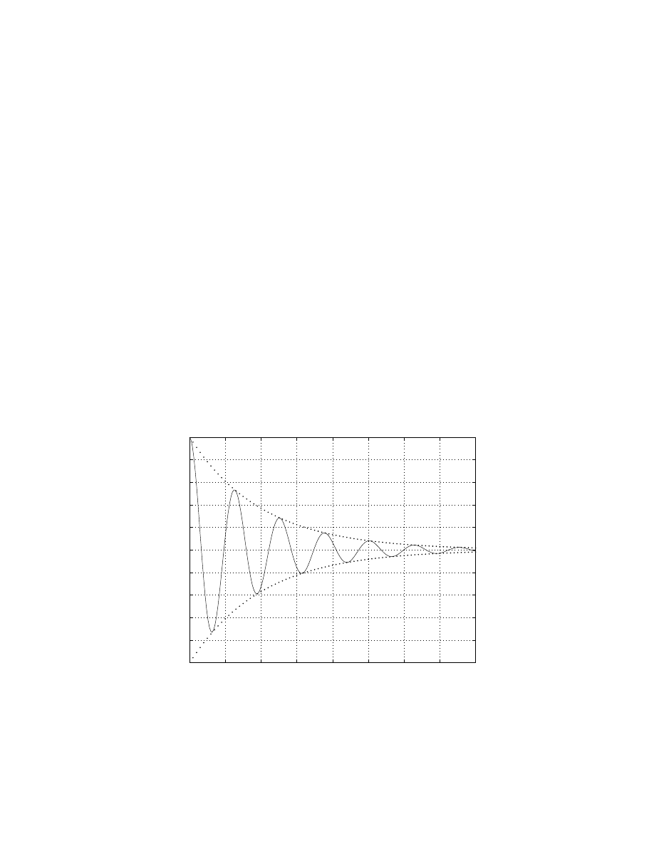
Example
2. (Decaying oscillation.) Find the solution to the IVP (Initial
Value Problem)
y
′′
+ 2y
′
+ 101y = 0,
y(0) = 1,
y
′
(0) = 0.
40
Answer.
The characteristic equation is
r
2
+ 2r + 101 = 0,
⇒
r
1,2
= −1 ± 10i, ⇒
λ = −1, µ = 10.
So the general solution is
y(t) = e
−t
(c
1
cos 10t + c
2
sin 10t),
so
y
′
(t) = −e
−t
(c
1
cos t + c
2
sin t) + e
−t
(−10c
1
sin t + 10c
2
cos t)
Fit in the ICs:
y(0) = 1 :
y(0) = e
0
(c
1
+ 0) = c
1
= 1,
y
′
(0) = 0 :
y
′
(0) = −1 + 10c
2
= 0,
c
2
= 0.1.
Solution is
y(t) = e
−t
(cos t + 0.1 sin t).
The graph is given below:
0
0.5
1
1.5
2
2.5
3
3.5
4
−1
−0.8
−0.6
−0.4
−0.2
0
0.2
0.4
0.6
0.8
1
We see it is a decaying oscillation. The sin and cos part gives the oscillation,
and the e
−t
part gives the decaying amplitude. As t → ∞, we have y → 0.
41
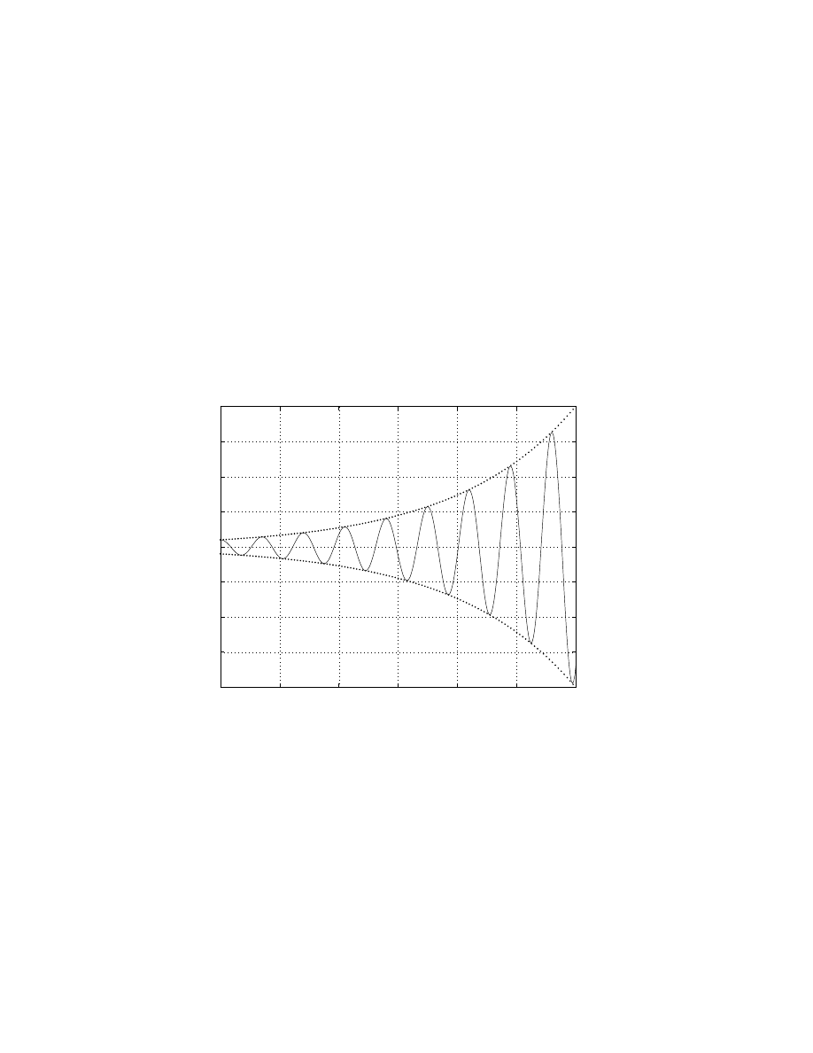
Example
3. (Growing oscillation) Find the general solution of y
′′
− y
′
+
81.25y = 0.
Answer.
r
2
− r + 81.25 = 0,
⇒
r = 0.5 ± 9i, ⇒
λ = 0.5,
µ = 2.
The general solution is
y(t) = e
0.5t
(c
1
cos 9t + c
2
sin 9t).
A typical graph of the solution looks like:
0
1
2
3
4
5
6
−20
−15
−10
−5
0
5
10
15
20
We see that y oscillate with growing amplitude as t grows. In the limit when
t → ∞, y oscillates between −∞ and +∞.
Conclusion:
Sign of λ, the real part of the complex roots, decides the type
of oscillation:
• λ = 0: perfect oscillation;
• λ < 0: decaying oscillation;
42

• λ > 0: growing oscillation.
We note that since λ =
−b
2a
, so the sign of λ follows the sign of −b.
43

3.4: Repeated roots; reduction of order
For the characteristic equation ar
2
+ br + c = 0, if b
2
= 4ac, we will have two
repeated roots
r
1
= r
2
= r = −
b
2a
.
We have one solution y
1
= e
rt
. How can we find the second solution which
is linearly independent of y
1
?
Example
1. Consider the equation y
′′
+4y
′
+4y = 0. We have r
2
+4r+4 = 0,
and r
1
= r
2
= r = −2. So one solution is y
1
= e
−2t
. What is y
2
?
Method 1.
Use Wronskian and Abel’s Theorem. By Abel’s Theorem we
have
W (y
1
, y
2
) = c exp(−
Z
4 dt) = ce
−4t
= e
−4t
,
(let c = 1).
By the definition of Wronskian we have
W (y
1
, y
2
) = y
1
y
′
2
− y
′
1
y
2
= e
−2t
y
′
2
− (−2)e
−2t
y
2
= e
−2t
(y
′
2
+ 2y
2
).
They must equal to each other:
e
−2t
(y
′
2
+ 2y
2
) = e
−4t
,
y
′
2
+ 2y
2
= e
−2t
.
Solve this for y
2
,
µ = e
2t
,
y
2
= e
−2t
Z
e
2t
e
−2t
dt = e
−2t
(t + C)
Let C = 0, we get y
2
= te
−2t
, and the general solution is
y(t) = c
1
y
1
+ c
2
y
2
= c
1
e
−2t
+ c
2
te
−2t
.
Method 2.
This is the textbook’s version. We guess a solution of the form
y
2
= v(t)y
1
= v(t)e
−2t
, and try to find the function v(t). We have
y
′
2
= v
′
e
−2t
+ v(−2e
−2t
) = e
−2t
(v
′
− 2v),
y
′′
2
= e
−2t
(v
′′
− 4v
′
+ 4v).
Put them in the equation
e
−2t
(v
′′
− 4v
′
+ 4v) + 4e
−2t
(v
′
− 2v) + 4v(t)e
−2t
= 0.
44
Cancel the term e
−2t
, and we get v
′′
= 0, which gives v(t) = c
1
t + c
2
. So
y
2
(t) = vy
1
= (c
1
t + c
2
)e
−2t
= c
1
te
−2t
+ c
2
e
−2t
.
Note that the term c
2
e
−2t
is already contained in cy
1
. Therefore we can choose
c
1
= 1, c
2
= 0, and get y
2
= te
−2t
, which gives the same general solution as
Method 1. We observe that this method involves more computation than
Method 1.
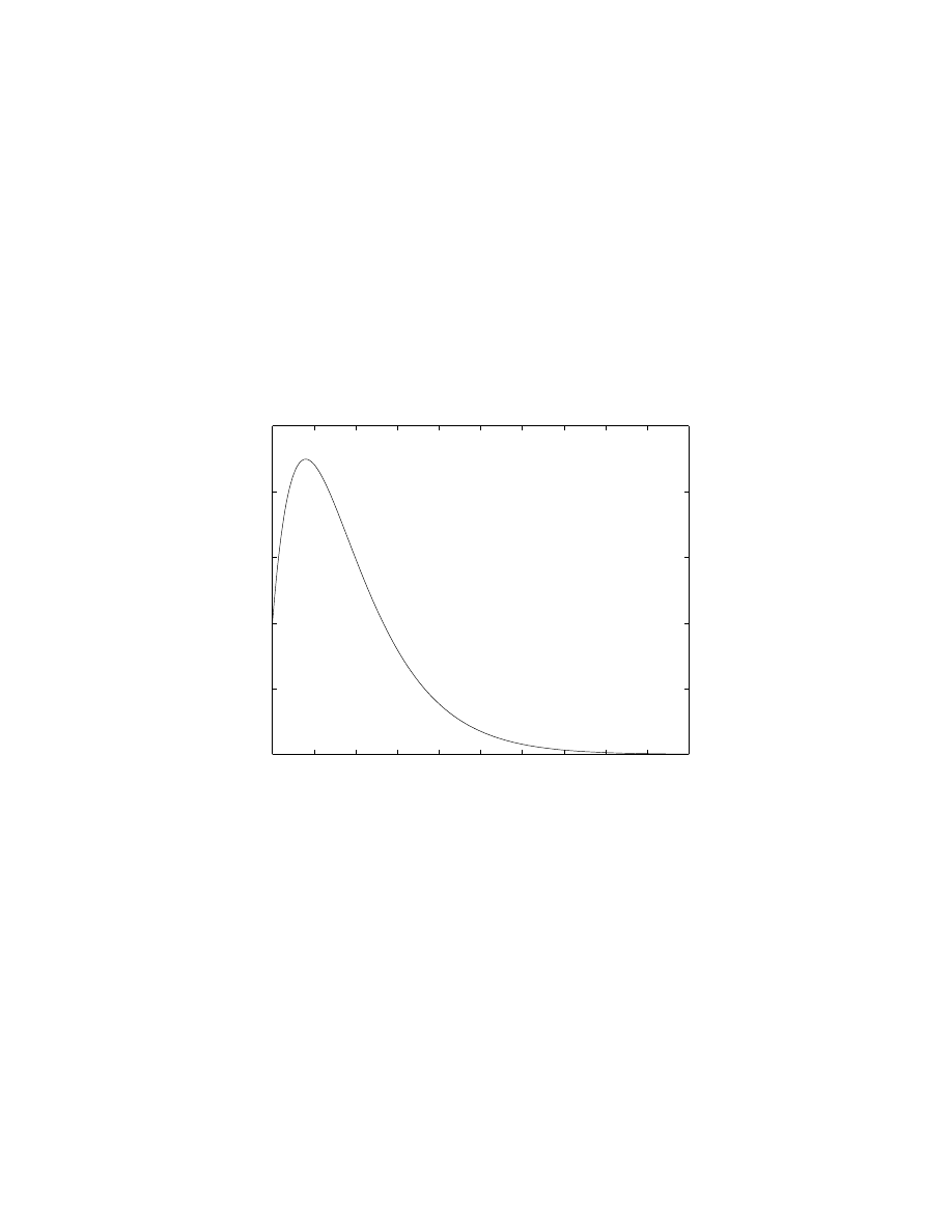
A typical solution graph is included below:
0
0.5
1
1.5
2
2.5
3
3.5
4
4.5
5
0
0.5
1
1.5
2
2.5
We see if c
2
> 0, y increases for small t. But as t grows, the exponential
(decay) function dominates, and solution will go to 0 as t → ∞.
One can show that in general if one has repeated roots r
1
= r
2
= r, then
y
1
= e
rt
and y
2
= te
rt
, and the general solution is
y = c
1
e
rt
+ c
2
tr
rt
= e
rt
(c
1
+ c
2
t).
Example
2. Solve the IVP
y
′′
− 2y
′
+ y = 0,
y(0) = 2,
y
′
(0) = 1.
45

Answer.
This follows easily now
r
2
− 2r + 1 = 0, ⇒
r
1
= r
2
= 1,
⇒
y(t) = (c
1
+ c
2
t)e
t
.
The ICs give
y(0) = 2 :
c
1
+ 0 = 2,
⇒
c
1
= 2.
y
′
(t) = (c
1
+ c
2
t)e
t
+ c
2
e
t
,
y
′
(0) = c
1
+ c
2
= 1,
⇒
c
2
= 1 − c
1
= −1.
So the solution is y(t) = (2 − t)e
t
.
Summary:
For ay
′′
+ by
′
+ cy = 0, and ar
2
+ br + c = 0 has two roots r
1
, r
2
,
we have
• If r
1
6= r
2
(real):
y(t) = c
1
e
r
1
t
+ c
2
e
r
2
t
;
• If r
1
= r
2
= r (real):
y(t) = (c
1
+ c
2
t)e
rt
;
• If r
1,2
= λ ± iµ complex:
y(t) = e
λt
(c
1
cos µt + c
2
sin µt).
More on reduction of order: This method can be used to find a second
solution y
2
if the first solution y
1
is given for a second order linear equation.
Example
3. For the equation
2t
2
y
′′
+ 3ty
′
− y = 0, t > 0,
given one solution y
1
=
1
t
, find a second linearly independent solution.
Answer.
Method 1
: Use Abel’s Theorem and Wronskian. By Abel’s
Theorem, and choose C = 1, we have
W (y
1
, y
2
) = exp
−
Z
p(t) dt
= exp
−
Z
3t
2t
2
dt
= exp
−
3
2
ln t
= t
−3/2
.
By definition of the Wronskian,
W (y
1
, y
2
) = y
1
y
′
2
− y
′
1
y
2
=
1
t
y
′
2
− (−
1
t
2
)y
2
= t
−3/2
.
46

Solve this for y
2
:
µ = exp(
Z
1
t
dt) = exp(ln t) = t,
⇒
y
2
=
1
t
Z
t · t
−
3
2
dt =
1
t
(
2
3
t
3
2
+ C).
Let C = 0, we get y
2
=
2
3
√
t. Since
2
3
is a constant multiplication, we can
drop it and choose y
2
=
√
t.
Method 2
: This is the textbook’s version. We saw in the previous example
that this method is inferior to Method 1, therefore we will not focus on it at
all. If you are interested in it, read the book.
Let’s introduce another method that combines the ideas from Method 1 and
Method 2.
Method 3.
We will use Abel’s Theorem, and at the same time we will seek
a solution of the form y
1
= vy
1
.
By Abel’s Theorem, we have ( worked out in M1) W (y
1
, y
2
) = t
−
3
2
. Now,
seek y
2
= vy
1
. By the definition of the Wronskian, we have
W (y
1
, y
2
) = y
1
y
′
2
− y
′
1
y
2
= y
1
(vy
1
)
′
− y
′
1
(vy
1
) = y
1
(v
′
y
1
+ vy
′′
1
) − vy
1
y
′
1
= v
′
y
2
1
.
Note that this is a general formula.
Now putting y
1
= 1/t, we get
v
′
1
t
2
= t
−
3
2
,
v
′
= t
1
2
,
v =
Z
t
1
2
dt =
2
3
t
3
2
.
Drop the constant
2
3
, we get
y
2
= vy
1
= t
3
2
1
t
= t
1
2
.
We see that Method 3 is the most efficient one among all three methods. We
will focus on this method from now on.
Example
4. Consider the equation
t
2
y
′′
− t(t + 2)y
′
+ (t + 2)y = 0,
t > 0.
47

Given y
1
= t, find the general solution.
Answer.
We have
p(t) = −
t(t + 2)
t
2
= −
t + 2
t
= −1 −
2
t
.
Let y
2
be the second solution. By Abel’s Theorem, choosing c = 1, we have
W (y
1
, y
2
) = exp
−
Z
(−1 −
2
t
)dt
= exp{t + 2 ln t} = t
2
e
t
.
Let y
2
= vy
1
, the W (y
1
, y
2
) = v
′
y
2
1
= t
2
v
′
. Then we must have
t
2
v
′
= t
2
e
t
,
v
′
= e
t
,
v = e
t
,
y
2
= te
t
.
(A cheap trick to double check your solution y
2
would be: plug it back into
the equation and see if it satisfies it.) The general solution is
y(t) = c
1
y
2
+ c
2
y
2
= c
1
t + c
2
te
t
.
We observe here that Method 3 is very efficient.
Example
5. Given the equation
t
2
y
′′
− (t −
3
16
)y = 0,
t > 0, and
y
1
= t
(1/4)
e
2
√
t
, find y
2
.
Answer.
We will always use method 3. We see that p = 0. By Abel’s
Theorem, setting c = 1, we have
W (y
1
, y
2
) = exp(
Z
0dt) = 1.
Seek y
2
= vy
1
. Then, W (y
1
, y
2
) = y
2
1
v
′
= t
1
2
e
4
√
t
v
′
. So we must have
t
1
2
e
4
√
t
v
′
= 1,
⇒
v
′
= t
−
1
2
e
−4
√
t
,
⇒
v =
Z
t
−
1
2
e
−4
√
t
dt.
Let u = −4
√
t, so du = −2t
−
1
2
dt, we have
v =
Z
−
1
2
e
u
du = −
1
2
e
u
= −
1
2
e
−4
√
t
.
So drop the constant −
1
2
, we get
y
2
= vy
1
= e
−4
√
t
t
1
4
e
2
√
t
= t
1
4
e
−2
√
t
.
The general solution is
y(t) = c
1
y
1
+ c
2
y
2
= t
1
4
(c
1
e
2
√
t
+ c
2
e
−2
√
t
).
48

3.6: Non-homogeneous equations; method of
undetermined coefficients
Want to solve the non-homogeneous equation
y
′′
+ p(t)y
′
+ q(t)y = g(t),
(N)
Steps:
1. First solve the homogeneous equation
y
′′
+ p(t)y
′
+ q(t)y = 0,
(H)
i.e., find y
1
, y
2
, linearly independent of each other, and form the general
solution
y
H
= c
1
y
1
+ c
2
y
2
.
2. Find a particular/specific solution Y for (N), by MUC (method of un-
determined coefficients);
3. The general solution for (N) is then
y = y
H
+ Y = c
1
y
1
+ c
2
y
2
+ Y.
Find c
1
, c
2
by initial conditions, if given.
Key step: step 2.
Why y = y
H
+ Y ?
A quick proof: If y
H
solves (H), then
y
′′
H
+ p(t)y
′
H
+ q(t)y
H
= 0,
(A)
and since Y solves (N), we have
Y
′′
+ p(t)Y
′
+ q(t)Y = g(t),
(B)
Adding up (A) and (B), and write y = y
H
+Y , we get y
′′
+p(t)y
′
+q(t)y = g(t).
Main focus: constant coefficient case, i.e.,
ay
′′
+ by
′
+ cy = g(t).
49

Example
1. Find the general solution for
y
′′
− 3y
′
+ 4y = 3e
2t
.
Answer.
Step 1: Find y
H
.
r
2
− 3r − 4 = (r + 1)(r − 4) = 0, ⇒
r
1
= −1, r
2
= 4,
so
y
H
= c
1
e
−t
+ c
2
e
4t
.
Step 2: Find Y . We guess/seek solution of the same form as the source term
Y = Ae
2t
, and will determine the coefficient A.
Y
′
= 2Ae
2t
,
Y
′′
= 4Ae
2t
.
Plug these into the equation:
4Ae
2t
− 3 · 2Ae
2t
− 4Ae
2t
= 3e
2t
,
⇒
−6A = 3, ⇒
A = −
1
2
.
So Y = −
1
2
e
2t
.
Step 3. The general solution to the non-homogeneous solution is
y(t) = y
H
+ Y = c
1
e
−t
+ c
2
e
4t
−
1
2
e
2t
.
Observation: The particular solution Y take the same form as the source
term g(t).
But this is not always true.
Example
2. Find general solution for
y
′′
− 3y
′
+ 4y = 2e
−t
.
Answer.
The homogeneous solution is the same as Example 1: y
H
= c
1
e
−t
+
c
2
e
4t
. For the particular solution Y , let’s first try the same form as g, i.e.,
Y = Ae
−t
. So Y
′
= −Ae
−t
, Y
′′
= Ae
−t
. Plug them back in to the equation,
we get
LHS = Ae
−t
− 3(−Ae
−t
) − 4Ae
−t
= 0 6= 2e
−et
= RHS.
So it doesn’t work. Why?
We see r
1
= −1 and y
1
= e
−t
, which means our guess Y = Ae
−t
is a solution
to the homogeneous equation. It will never work.
50

Second try: Y = Ate
−t
. So
Y
′
= Ae
−t
− Ate
−t
,
Y
′′
= −Ae
−t
− Ae
−t
+ Ate
−t
= −2Ae
−t
+ Ate
−t
.
Plug them in the equation
(−2Ae
−t
+ Ate
−t
) − 3(Ae
−t
− Ate
−t
) − 4Ate
−t
= −5Ae
−t
= 2e
−t
,
we get
−5A = 2, ⇒
A = −
2
5
,
so we have Y = −
2
5
te
−t
.
Summary 1.
If g(t) = ae
αt
, then the form of the particular solution Y
depends on r
1
, r
2
(the roots of the characteristic equation).
case
form of the particular solution Y
r
1
6= α and r
2
6= α
Y = Ae
αt
r
1
= α or r
2
= α, but r
1
6= r
2
Y = Ate
αt
r
1
= r
2
= α
Y = At
2
e
αt
Example
3. Find the general solution for
y
′′
− 3y
′
− 4y = 3t
2
+ 2.
Answer.
The y
H
is the same y
H
= c
1
e
−t
+ c
2
e
4t
.
Note that g(t) is a polynomial of degree 2. We will try to guess/seek a
particular solution of the same form:
Y = At
2
+ Bt + C,
Y
′
= 2At + B,
Y
′′
= 2A
Plug back into the equation
2A−3(2At+b)−4(At
2
+Bt+C) = −4At
2
−(6A+4B)t+(2A−3B−4C) = 3t
2
+2.
51

Compare the coefficient, we get three equations for the three coefficients
A, B, C:
−4A = 3
→ A = −
3
4
−(6A + 4B) = 0, → B =
9
8
2A − 3B − 4C = 2, → C =
1
4
(2A − 3B − 2) = −
55
32
So we get
Y (t) = −
3
4
t
2
+
9
8
t −
55
32
.
But sometimes this guess won’t work.
Example
4. Find the particular solution for y
′′
− 3y
′
= 3t
2
+ 2.
Answer.
We see that the form we used in the previous example Y =
At
2
+ Bt + C won’t work because Y
′′
− 3Y
′
will not have the term t
2
.
New try: multiply by a t. So we guess Y = t(At
2
+ Bt+ C) = At
3
+ Bt
2
+ Ct.
Then
Y
′
= 3At
2
+ 2Bt + C,
Y
′′
= 6At + 2B.
Plug them into the equation
(6At + 2B) −3(3At
2
+ 2Bt + C) = −9At
2
+ (6A −6B)t+(2B −3C) = 3t
2
+ 2.
Compare the coefficient, we get three equations for the three coefficients
A, B, C:
−9A = 3
→ A = −
1
3
(6A − 6B) = 0, → B = A = −
1
3
2B − 3C = 2, → C =
1
3
(2B − 2) = −
8
9
So Y = t(−
1
3
t
2
−
1
3
t −
8
9
).
52
Summary 2.
If g(t) is a polynomial of degree n, i.e.,
g(t) = α
n
t
n
+ · · · + α
1
t + α
0
the particular solution for
ay
′′
+ by
′
+ cy = g(t)
(where a 6= 0) depends on b, c:
case
form of the particular solution Y
c 6= 0
Y = P
n
(t) = A
n
t
n
+ · · · + A
1
t + A
0
c = 0 but b 6= 0
Y = tP
n
(t) = t(A
n
t
n
+ · · · + A
1
t + A
0
)
c = 0 and b = 0 Y = t
2
P
n
(t) = t
2
(A
n
t
n
+ · · · + A
1
t + A
0
)
Example
5. Find a particular solution for
y
′′
− 3y
′
− 4y = sin t.
Answer.
Since g(t) = sin t, we will try the same form. Note that (sin t)
′
=
cos t, so we must have the cos t term as well. So the form of the particular
solution is
Y = A sin t + B cos t.
Then
Y
′
= A cos t − B sin t,
Y
′′
= −A sin t − B cos t.
Plug back into the equation, we get
(−A sin t − B cos t) − 3(A cos t − B sin t) − 4(A sin t + b cos t)
= (−5A + 3B) sin t + (−3A − 5B) cos t = sin t.
So we must have
−5A + 3B = 1, −3A − 5B = 0,
→
A =
5
34
,
B =
3
34
.
So we get
Y (t) = −
5
34
sin t +
3
34
cos t.
53
But this guess won’t work if the form is a solution to the homogeneous
equation.
Example
6. Find a general solution for y
′′
+ y = sin t.
Answer.
Let’s first find y
H
. We have r
2
+ 1 = 0, so r
1,2
= ±i, and
y
H
= c
1
cos t + c
2
sin t.
For the particular solution Y : We see that the form Y = A sin t + B cos t
won’t work because it solves the homogeneous equation.
Our new guess: multiply it by t, so
Y (t) = t(A sin t + B cos t).
Then
Y
′
= (A sin t + B cos t) + t(A cos t + B sin t),
Y
′′
= (−2B − At) sin t + (2A − Bt) cos t.
Plug into the equation
Y
′′
+ Y = −2B sin t + 2A cos t = sin t,
⇒
A = 0, B = −
1
2
So
Y (y) = −
1
2
t cos t.
The general solution is
y(t) = y
H
+ Y = c
1
cos t + c
2
sin t −
1
2
t cos t.
Summary 3.
If g(t) = a sin αt + b cos αt, the form of the particular solution
depends on the roots r
1
, r
2
.
case
form of the particular solution Y
r
1,2
6= ±αi
Y = A sin αt + B cos αt
r
1,2
= ±αi
Y = t(A sin αt + B cos αt)
Next we study a couple of more complicated forms of g.
54

Example
7. Find a particular solution for
y
′′
− 3y
′
− 4y = te
t
.
Answer.
We see that g = P
1
(t)e
at
, where P
1
is a polynomial of degree 1.
Also we see r
1
= −1, r
2
= 4, so r
1
6= a and r
2
6= a. For a particular solution
we will try the same form as g, i.e., Y = (At + B)e
t
. So
Y
′
= Ae
t
+ (At + b)e
t
= (A + b)e
t
+ Ate
t
,
Y
′′
= · · · = (2A + B)e
t
+ Ate
t
.
Plug them into the equation,
[(2A+B)e
t
+Ate
t
]−3[(A+b)e
t
+Ate
t
]−4(At+B)e
t
= (−6At−A−6B)e
t
= te
t
.
We must have −6At − A − 6B = t, i.e.,
−6A = 1, −A−6B = 0, ⇒
A = −
1
6
, B =
1
36
,
⇒
Y = (−
1
6
t+
1
36
)e
t
.
However, if the form of g is a solution to the homogeneous equation, it won’t
work for a particular solution. We must multiply it by t in that case.
Example
8. Find a particular solution of
y
′′
− 3y
′
− 4y = te
−t
.
Answer.
Since a = −1 = r
1
, so the form we used in Example 7 won’t work
here. Try
Y = t(At + B)e
−t
= (At
2
+ Bt)e
−t
.
Then
Y
′
= · · · = [−At
2
+ (2A − B)t + B]e
−t
,
Y
′′
= · · · = [At
2
+ (B − 4A)t + 2A − 2B]e
−t
.
Plug into the equation
[At
2
+ (B − 4A)t + 2A − 2B]e
−t
− 3[−At
2
+ (2A − B)t + B]e
−t
− 4(At
2
+ Bt)e
−t
= [−10At + 2A − 5B]e
−t
= te
t
.
55
So we must have −10At + 2A − 5B = t, which means
−10A = 1, 2A − 5B = 0,
⇒
A = −
1
10
, B = −
1
25
.
Then
Y =
−
1
10
t
2
−
1
25
t
e
−t
.
Summary 4.
If g(t) = P
n
(t)e
at
where P
n
(t) = α
n
t
n
+ · · · + α
1
t + α
0
is a
polynomial of degree n, then the form of a particular solution depends on
the roots r
1
, r
2
.
case
form of the particular solution Y
r
1
6= a and r
2
6= a
Y = ˜
P
n
(t)e
at
= (A
n
t
n
+ · · · + A
1
t + A
0
)e
at
r
1
= a or r
2
= a but r
1
6= r
2
Y = t ˜
P
n
(t)e
at
= t(A
n
t
n
+ · · · + A
1
t + A
0
)e
at
r
1
= r
2
= a
Y = t
2
˜
P
n
(t)e
at
= t
2
(A
n
t
n
+ · · · + A
1
t + A
0
)e
at
Other cases of g are treated in a similar way: Check if the form of g is a
solution to the homogeneous equation. If not, then use it as the form of a
particular solution. If yes, then multiply it by t or t
2
.
We summarize a few cases below.
Summary 5.
If g(t) = e
αt
(a cos βt + b sin βt), and r
1
, r
2
are the roots of the
characteristic equation. Then
case
form of the particular solution Y
r
1,2
6= α ± iβ
Y = e
αt
(A cos βt + B sin βt)
r
1,2
= α ± iβ
Y = t · e
αt
(A cos βt + B sin βt)
Summary 6.
If g(t) = P
n
(t)e
αt
(a cos βt + b sin βt) where P
n
(t) is a poly-
nomial of degree n, and r
1
, r
2
are the roots of the characteristic equation.
Then
56

case
form of the particular solution Y
r
1,2
6= α ± iβ
Y = e
αt
[(A
n
t
n
+ · · · + A
0
) cos βt + (B
n
t
n
+ · · · + B
0
) sin βt]
r
1,2
= α ± iβ Y = t · e
αt
[(A
n
t
n
+ · · · + A
0
) cos βt + (B
n
t
n
+ · · · + B
0
) sin βt]
If the source g(t) has several terms, we treat each separately and add up
later. Let g(t) = g
1
(t) + g
2
(t) + · · · g
n
(t), then, find a particular solution Y
i
for each g
i
(t) term as if it were the only term in g, then Y = Y
1
+ Y
2
+ · · · Y
n
.
This claim follows from the principle of superposition.
In the examples below, we want to write the form of a particular solution.
Example
9.
y
′′
− 3y
′
− 4y = sin 4t + 2e
4t
+ e
5t
− t.
Answer.
Since r
1
= −1, r
2
= 2, we treat each term in g separately and the
add up:
Y (t) = A sin 4t + B cos 4tCte
4t
+ De
5t
+ (Et + F ).
Example
10.
y
′′
+ 16y = sin 4t + cos t − 4 cos 4t + 4.
Answer.
The char equation is r
2
+ 16 = 0, with roots r
1,2
= ±4i, and
y
H
= c
1
sin 4t + c
2
cos 4t.
We also note that the terms sin 4t and −4 cos 4t are of the same type, and
we must multiply it by t. So
Y = t(A sin 4t + B cos 4t) + (C cos t + D sin t) + E.
Example
11.
y
′′
− 2y
′
+ 2y = e
t
cos t + 8e
t
sin 2t + te
−t
+ 4e
−t
+ t
2
− 3.
Answer.
The char equation is r
2
− 2r + 2 = 0 with roots r
1,2
= 1 ± i. Then,
for the term e
t
cos t we must multiply by t.
Y = te
t
(A
1
cos t+A
2
sin t)+e
t
(B
1
cos 2t+B
2
sin 2t)+(C
1
t+C
0
)e
−t
+De
−t
+(F
2
t
2
+F
1
t+F
0
).
57
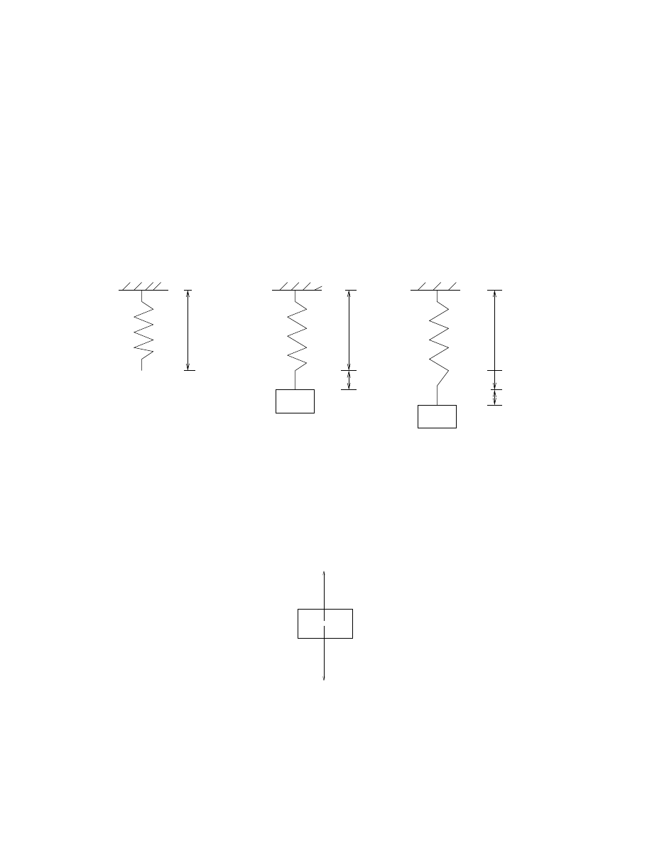
3.7: Mechanical vibrations
In this chapter we study some applications of the IVP
ay
′′
+ by
′
+ cy = g(t),
y(0) = y
0
,
y
′
(0) = ¯
y
0
.
The spring-mass system: See figure below.
(C)
l
l
L
l+L
extra
stretch
(A)
(B)
Figure (A): a spring in rest, with length l.
Figure (B): we put a mass m on the spring, and the spring is stretched. We
call length L the elongation
Figure (C): The spring-mass system is set in motion by stretch/squueze it
extra, with initial velocity, or with external force.
Force diagram at equilibrium position: mg = F s.
F
mg
s
Hooke’s law: Spring force F
s
= −kL, where L =elongation and k =spring
constant.
58

So: we have mg = kL which give
k =
mg
L
which gives a way to obtain k by experiment: hang a mass m and measure
the elongation L.
Model the motion: Let u(t) be the displacement/position of the mass at time
t, assuming the origin u = 0 at the equilibrium position, and downward the
positive direction.
Total elongation: L + u
Total spring force: F
s
= −k(L + u)
Other forces:
* damping/resistent force: F
d
(t) = −γv = −γu
′
(t), where γ is the damping
constant, and v is the velocity
* External force applied on the mass: F (t), given function of t
Total force on the mass:
P f = mg + F
s
+ F
d
+ F .
Newton’s law of motion ma =
P f gives
ma = mu
′′
=
X
f = mg + F
s
+ F
d
+ F,
mu
′′
= mg − k(L + u) − γu
′
+ F.
Since mg = kL, by rearranging the terms, we get
mu
′′
+ γu
′
+ ku = F
where m ia the mass, γ is the damping constant, k is the spring constant,
and F is the external force.
Next we study several cases.
Case 1: Undamped free vibration (simple harmonic motion). We assume no
damping (γ = 0) and no external force (F = 0). So the equation becomes
mu
′′
+ ku = 0.
Solve it
mr
2
+ k = 0,
r
2
= −
k
m
,
r
1,2
= ±
r k
m
i = ±ω
0
i,
where ω
0
=
r k
m
.
59
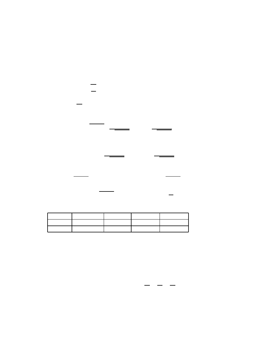
General solution
u(t) = c
1
cos ω
0
t + c
2
sin ω
0
t.
Four terms of this motion, frequency, period, amplitude and phase, defined
below:
Frequency: ω
0
=
r k
m
Period: T =
2π
ω
0
Amplitude and phase: We need to work on this a bit. We can write
u(t) =
q
c
2
1
+ c
2
2
c
1
pc
2
1
+ c
2
2
cos ω
0
t +
c
2
pc
2
1
+ c
2
2
sin ω
0
t
!
.
Now, define δ, such that tan δ = c
2
/c
1
, then
sin δ =
c
2
pc
2
1
+ c
2
2
,
cos δ =
c
1
pc
2
1
+ c
2
2
so we have
u(t) =
q
c
2
1
+ c
2
2
(cos δ · cos ω
0
t + sin δ · sin ω
0
t) =
q
c
2
1
+ c
2
2
cos(ω
0
t − δ).
So amplitude is R =
pc
2
1
+ c
2
2
and phase is δ = arctan
c
2
c
1
.
A few words on units:
force (f )
weight (mg)
length (u)
mass (m)
gravity (g)
lb
lb
ft
lb · sec
2
/ft
32 ft/sec
2
newton
newton
m
kg
9.8 m/sec
2
Example
1. A mass weighing 10 lb stretches a spring 2 in. If the mass is
displaced an additional 2 in, and is then set in motion with initial upward
velocity of 1 ft/sec, determine the position, frequency, period, amplitude and
phase of the motion.
Answer.
We see this is free harmonic oscillation. We have
mg = 10,
g = 32,
m =
10
g
=
10
32
=
5
16
.
60

And the elongation is L = 2in =
1
6
ft. So k = mg/L = 60. Let u(t) be the
position from equilibrium, we get the equation
mu
′′
+ ku = 0,
5
16
u
′′
+ 60u = 0,
therefore
u
′′
+ 192u = 0,
u(0) =
1
6
, u
′
(0) = −1.
So the frequency is ω
0
=
√
192, and the general solution is
u(t) = c
1
cos ω
0
t + c
2
sin ω
0
t
By the ICs:
u(0) = c
1
=
1
6
,
u
′
(0) = ω
0
c
2
= −1,
c
2
= −
1
ω
0
= −
1
√
192
.
(Note that c
1
= u(0) and c
2
= u
′
(0)/ω
0
.) Now we have the position at any
time t
u(t) =
1
6
cos ω
0
t −
1
√
192
sin ω
0
t.
The four terms of the motion are
ω
0
=
√
192,
T =
2π
ω
0
=
π
√
48
,
R =
q
c
2
1
+ c
2
2
=
r 19
576
≈ 0.18,
and
δ = arctan
c
2
c
1
= arctan −
6
√
192
= − arctan
√
3
4
.
Case II: Damped free vibration. We assume that γ 6= 0(> 0) and F = 0.
mu
′′
+ γu
′
+ ku = 0
then
mr
2
+ γr + k = 0,
r
1,2
=
−γ ±
pγ
2
− 4km
2m
.
We see the type of root depends on the sign of γ
2
− 4km.
61

• If γ
2
− 4km > 0, (i.e., γ >
√
4km) we have two real roots, and the
general solution is u = c
1
e
r
1
t
+ c
2
e
r
2
t
, with r
1
< 0, r
2
< 0.
Due to the large damping force, there will be no vibration in the motion.
The mass will simply return to the equilibrium position exponentially.
This kind of motion is called overdamped.
• If γ
2
−4km = 0, (i.e., γ =
√
4km) we have double roots r
1
= r
2
= r < 0.
So u = (c
1
+ c
2
t)e
rt
.
Depending on the sign of c
1
, c
2
(which is determined by the ICs), the
mass may cross the equilibrium point maximum once. This kind of mo-
tion is called critically damped, and this value of γ is called critical
damping
.
• If γ
2
− 4km < 0, (i.e., γ <
√
4km) we have complex roots
r
1,2
= −λ ± µi, λ =
γ
2m
,
µ =
p4km − γ
2
2m
.
So the position is
u = e
−λt
(c
1
cos µt + c
2
sin µt).
This motion is damped oscillation. We can write
u(t) = e
−λt
R · cos(µt − δ),
R =
q
c
2
1
+ c
2
2
,
δ = arctan
c
2
c
1
.
Here the term e
−λt
R is the amplitude, and µ is called the quasi fre-
quency, and the quasi period is
2π
µ
. The graph of the solution looks like
the one for complex roots with negative real part.
Summary
: For all cases, since the real part of the roots are always negative,
u will go to zero as t grow. This means, if there is damping, no matter how
big or small, the motion will eventually come to a rest.
Example
2. A mass of 9.8 kg is hanging on a spring with k = 1. The mass
is in a medium that exerts a viscous resistance of 6 lb when the mass has a
62

velocity of 48 ft/s. The mass is then further stretched for another 2ft, then
released from rest. Find the position u(t) of the mass.
Answer.
We have γ =
6
48
=
1
8
. So the equation for u is
mu
′′
+ γu
′
+ ku = 0,
u
′′
+
1
8
u
′
+ u = 0,
u(0) = 2,
u
′
(0) = 0.
Solve it
r
2
+
1
8
r + 1 = 0,
r
1,2
= −
1
16
±
√
255
16
i,
ω
0
=
√
255
16
u(t) = e
−
1
16
t
(c
1
cos ω
0
t + c
2
sin ω
0
t).
By ICs, we have u(0) = c
1
= 2, and
u
′
(t) = −
1
16
u(t) + e
−
1
16
t
(−ω
0
c
1
sin ω
0
t + ω
0
c
2
cos ω
0
t),
u
′
(0) = −
1
16
u(0) + ω
0
c
2
= 0,
c
2
=
2
√
255
.
So the position at any time t is
u(t) = e
−t/16
(2 cos ω
0
t −
2
√
255
sin ω
0
t).
63

3.9: Forced vibrations
In this chapter we assume the external force is F (t) = F
0
cos ωt. (The case
where F (t) = F
0
sin ωt is totally similar.)
Case 1
: With damping.
mu
′′
+ γu
′
+ ku = F
0
cos ωt.
Solution consists of two parts:
u = u
H
+ U,
u
H
: the solution of the homogeneous equation,
U: a particular solution.
From discussion is the previous chapter, we know that u
H
→ 0 as t → ∞
for systems with damping. Therefore, this part of the solution is called the
transient solution.
The appearance of U is due to the force term F . Therefore it is called the
forced response. The form is U = R cos(ωt − δ). We see it is a periodic
oscillation for all time t.
As time t → ∞, we have u → U. So U is called the steady state.
Case 2
: Without damping.
mu
′′
+ ku = F
0
cos ωt
ω
0
=
r k
m
,
u
H
= c
1
cos ω
0
t + c
2
sin ω
0
t
The form of the particular solution depends on the value of w. We have two
cases.
Case 2A
: if w 6= w
0
. The particular solution should be
U = A cos wt + B cos wt
But there is no u
′
term, so we only need U = A cos wt. And U
′′
= −w
2
A cos wt.
Plug in the equation
m(−w
2
A cos wt) + kA cos wt = F
0
cos wt,
64
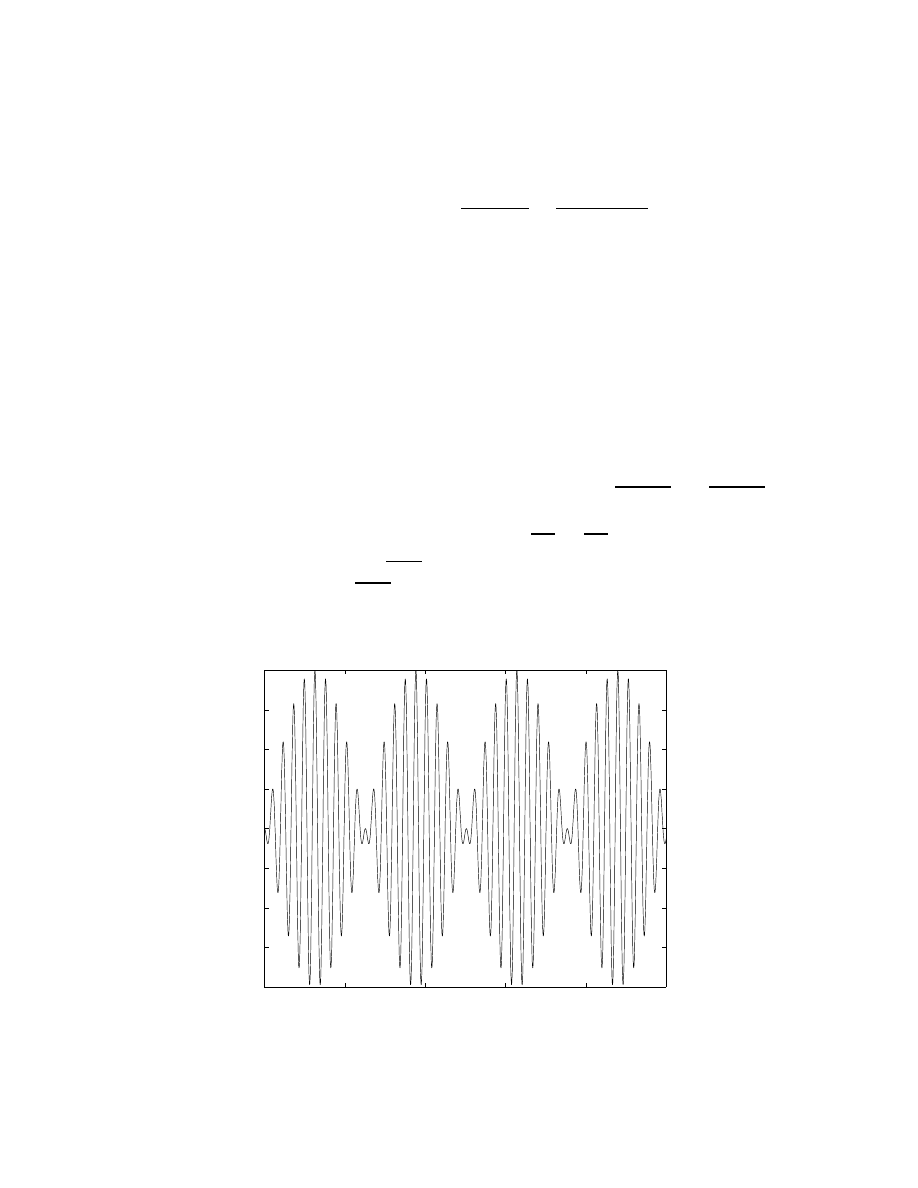
(k − mw
2
)A = F
0
,
A =
F
0
k − mw
2
=
F
0
m(w
2
0
− w
2
)
.
General solution
u(t) = c
1
cos w
0
t + c
2
sin w
0
t + A cos wt
Assume ICs: u(0) = 0, u
′
(0) = 0. Find c
1
, c
2
.
u(0) = 0 :
c
1
+ A = 0,
c
1
= −A
u
′
(0) = 0 :
0 + w
0
c
2
+ 0 = 0,
c
2
= 0
Solution
u(t) = −A cos w
0
t+A cos wt = A(cos wt−cos w
0
t) = 2A sin
w
0
− w
2
t·sin
w
0
+ w
2
t.
(We used the trig identity: cos a − cos b = 2 sin
b−a
2
sin
a+b
2
.)
We see the first term 2A sin
w
0
−w
2
t can be viewed as the varying amplitude,
and the second term sin
w
0
+w
2
t is the vibration.
One particular situation: if w
0
6= w but w
o
≈ w, then |w
0
− w| << |w
0
+ w|.
The plot looks like (we choose w
0
= 9, w = 10)
0
5
10
15
20
25
−2
−1.5
−1
−0.5
0
0.5
1
1.5
2
65
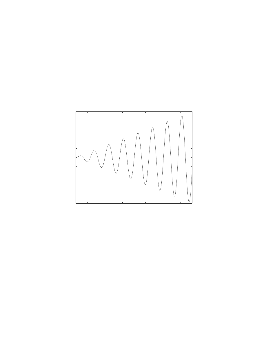
This is called a beat. (One observes it by hitting two nearby keys on a piano,
for example.)
Case 2B
: If w = w
0
. The particular solution is
U = At cos w
0
t + Bt sin w
0
t
A typical plot looks like:
0
0.5
1
1.5
2
2.5
3
3.5
4
4.5
5
−5
−4
−3
−2
−1
0
1
2
3
4
5
This is called resonance. If the frequency of the source term ω equals to the
frequency of the system ω
0
, then, small source term could make the solution
grow very large!
Summary
:
• With damping: Transient solution plus the forced response term,
• Without damping:
if w = w
0
: resonance.
if w 6= w
0
but w ≈ w
0
: beat.
66

Chapter 6. The Laplace Transform
—used to handle piecewise continuous or impulsive force.
6.1: Definition of the Laplace transform
Topics:
• Definition of Laplace transform,
• Compute Laplace transform by definition, including piecewise contin-
uous functions.
Definition:
Given a function f (t), t ≥ 0, its Laplace transform F (s) =
L{f(t)} is defined as
F (s) = L{f(t)}
.
=
Z
∞
0
e
−st
f (t) dt
.
= lim
A→∞
Z
A
0
e
−st
f (t) dt
We say the transform converges if the limit exists, and diverges if not.
Next we will give examples on computing the Laplace transform of given
functions by definition.
Example
1. f (t) = 1 for t ≥ 0.
Answer.
F (s) = L{f(t)} = lim
A→∞
Z
A
0
e
−st
dt = lim
A→∞
−
1
s
e
−st
A
0
= lim
A→∞
−
1
s
e
−sA
− 1
=
1
s
,
(s > 0)
Example
2. f (t) = e
t
.
Answer.
F (s) = L{f(t)} = lim
A→∞
Z
A
0
e
−st
e
at
dt = lim
A→∞
Z
A
0
e
−(s−a)t
dt = lim
A→∞
−
1
s − a
e
−(s−a)t
A
0
=
lim
A→∞
−
1
s − a
e
−(s−a)A
− 1
=
1
s − a
,
(s > a)
67

Example
3. f (t) = t
n
, for n ≥ 1 integer.
Answer.
F (s) =
lim
A→∞
Z
A
0
e
−st
t
n
dt =
lim
A→∞
(
t
n
e
−st
−s
A
0
−
Z
A
0
nt
n−1
e
−st
−s
dt
)
= 0 +
n
s
lim
A→∞
Z
A
0
e
−st
t
n−1
dt =
n
s
L{t
n−1
}.
So we get a recursive relation
L{t
n
} =
n
s
L{t
n−1
}, ∀n,
which means
L{t
n−1
} =
n − 1
s
L{t
n−2
}, L{t
n−2
} =
n − 2
s
L{t
n−3
}, · · ·
By induction, we get
L{t
n
} =
n
s
L{t
n−1
} =
n
s
(n − 1)
s
L{t
n−2
} =
n
s
(n − 1)
s
(n − 2)
s
L{t
n−3
}
= · · · =
n
s
(n − 1)
s
(n − 2)
s
· · ·
1
s
L{1} =
n!
s
n
1
s
=
n!
s
n+1
,
(s > 0)
Example
4. Find the Laplace transform of sin at and cos at.
Answer.
Method 1. Compute by definition, with integration-by-parts,
twice. (lots of work...)
Method 2. Use the Euler’s formula
e
iat
= cos at + i sin at,
⇒
L{e
iat
} = L{cos at} + iL{sin at}.
By Example 2 we have
L{e
iat
} =
1
s − ia
=
1(s + ia)
(s − ia)(s + ia)
=
s + ia
s
2
+ a
2
=
s
s
2
+ a
2
+ i
a
s
2
+ a
2
.
Comparing the real and imaginary parts, we get
L{cos at} =
s
s
2
+ a
2
,
L{sin at} =
a
s
2
+ a
2
,
(s > 0).
68

Remark: Now we will use
R
∞
0
instead of lim
A→∞
R
A
0
, without causing confu-
sion.
For piecewise continuous functions, Laplace transform can be computed by
integrating each integral and add up at the end.
Example
5. Find the Laplace transform of
f (t) =
1,
0 ≤ t < 2,
t − 2, 2 ≤ t.
We do this by definition:
F (s) =
Z
∞
0
e
−st
f (t) dt =
Z
2
0
e
−st
dt +
Z
∞
2
(t − 2)e
−st
dt
=
1
−s
e
−st
2
t=0
+ (t − 2)
1
−s
e
−st
∞
t=2
−
Z
A
2
1
−s
e
−st
dt
=
1
−s
(e
−2s
− 1) + (0 − 0) +
1
s
1
−s
e
−st
∞
t=2
=
1
−s
(e
−2s
− 1) +
1
s
2
e
−2s
69

6.2: Solution of initial value problems
Topics:
• Properties of Laplace transform, with proofs and examples
• Inverse Laplace transform, with examples, review of partial fraction,
• Solution of initial value problems, with examples covering various cases.
Properties of Laplace transform:
1. Linearity: L{c
1
f (t) + c
2
g(t)} = c
1
L{f(t)} + c
2
L{g(t)}.
2. First derivative: L{f
′
(t)} = sL{f(t)} − f(0).
3. Second derivative: L{f
′′
(t)} = s
2
L{f(t)} − sf(0) − f
′
(0).
4. Higher order derivative:
L{f
(n)
(t)} = s
n
L{f(t)}−s
n−1
f (0)−s
n−2
f
′
(0)−· · ·−sf
(n−2)
(0)−f
(n−1)
(0).
5. L{−tf(t)} = F
′
(s) where F (s) = L{f(t)}. This also implies L{tf(t)} =
−F
′
(s).
6. L{e
at
f (t)} = F (s − a) where F (s) = L{f(t)}. This implies e
at
f (t) =
L
−1
{F (s − a)}.
Remarks:
• Note property 2 and 3 are useful in differential equations. It shows
that each derivative in t caused a multiplication of s in the Laplace
transform.
• Property 5 is the counter part for Property 2. It shows that each
derivative in s causes a multiplication of −t in the inverse Laplace
transform.
• Property 6 is also known as the Shift Theorem. A counter part of it
will come later in chapter 6.3.
70

Proof:
1. This follows by definition.
2. By definition
L{f
′
(t)} =
Z
∞
0
e
−st
f
′
(t)dt = e
−st
f (t)
∞
0
−
Z
∞
0
(−s)e
−st
f (t)dt = −f(0)+sL{f(t)}.
3. This one follows from Property 2. Set f to be f
′
we get
L{f
′′
(t)} = sL{f
′
(t)}−f
′
(0) = s(sL{f(t)}−f(0))−f
′
(0) = s
2
L{f(t)}−sf(0)−f
′
(0).
4. This follows by induction, using property 2.
5. The proof follows from the definition:
F
′
(s) =
d
ds
Z
∞
0
e
−st
f (t)dt =
Z
∞
0
∂
∂s
(e
−st
)f (t)dt =
Z
∞
0
(−t)e
−st
f (t)dt = L{−tf(t)}.
6. This proof also follows from definition:
L{e
at
f (t)}
Z
∞
0
e
−st
e
at
f (t)dt =
Z
∞
0
e
−(s−a)t
f (t)dt = F (s − a).
By using these properties, we could find more easily Laplace transforms of
many other functions.
Example
1.
From
L{t
n
} =
n!
s
n+1
,
we get
L{e
at
t
n
} =
n!
(s − a)
n+1
.
Example
2.
From
L{sin bt} =
b
s
2
+ b
2
,
we get
L{e
at
sin bt} =
b
(s − a)
2
+ b
2
.
71

Example
3.
From
L{cos bt} =
s
s
2
+ b
2
,
we get
L{e
at
cos bt} =
s − a
(s − a)
2
+ b
2
.
Example
4.
L{t
3
+ 5t − 2} = L{t
3
} + 5L{t} − 2L{1} =
3!
s
4
+ 5
1
s
2
− 2
1
s
.
Example
5.
L{e
2t
(t
3
+ 5t − 2)} =
3!
(s − 2)
4
+ 5
1
(s − 2)
2
− 2
1
s − 2
.
Example
6.
L{(t
2
+ 4)e
2t
− e
−t
cos t} =
2
(s − 2)
3
+
4
s − 2
−
s + 1
(s + 1)
2
+ 1
,
because
L{t
2
+ 4} =
2
s
3
+
4
s
,
⇒
L{(t
2
+ 4)e
2t
} =
2
(s − 2)
3
+
4
s − 2
.
Next are a few examples for Property 5.
Example
7.
Given L{e
at
} =
1
s − a
,
we get
L{te
at
} = −
1
s − a
′
=
1
(s − a)
2
Example
8.
L{t sin bt} = −
b
s
2
+ b
2
′
=
−2bs
(s
2
+ b
2
)
2
.
Example
9.
L{t cos bt} = −
s
s
2
+ b
2
′
= · · · =
s
2
− b
2
(s
2
+ b
2
)
2
.
72

Inverse Laplace transform
. Definition:
L
−1
{F (s)} = f(t),
if
F (s) = L{f(t)}.
Technique: find the way back.
Some simple examples:
Example
10.
L
−1
3
s
2
+ 4
= L
−1
3
2
·
2
s
2
+ 2
2
=
3
2
L
−1
2
s
2
+ 2
2
=
3
2
sin 2t.
Example
11.
L
−1
2
(s + 5)
4
= L
−1
1
3
·
6
(s + 5)
4
=
1
3
L
−1
3!
(s + 5)
4
=
1
3
e
−5t
L
−1
3!
s
4
=
1
3
e
−5t
t
3
.
Example
12.
L
−1
s + 1
s
2
+ 4
= L
−1
s
s
2
+ 4
+
1
2
L
−1
2
s
2
+ 4
= cos 2t
1
2
sin 2t.
Example
13.
L
−1
s + 1
s
2
− 4
= L
−1
s + 1
(s − 2)(s + 2)
= L
−1
3/4
s − 2
+
1/4
s + 2
=
3
4
e
2t
+
1
4
e
−2t
.
Here we used partial fraction to find out:
s + 1
(s − 2)(s + 2)
=
A
s − 2
+
B
s + 2
,
A = 3/4,
B = 1/4.
73

Solutions of initial value problems.
We will go through one example first.
Example
14. (Two distinct real roots.) Solve the initial value problem by
Laplace transform,
y
′′
− 3y
′
− 10y = 2,
y(0) = 1, y
′
(0) = 2.
Answer.
Step 1. Take Laplace transform on both sides: Let L{y(t)} =
Y (s), and then
L{y
′
(t)} = sY (s)−y(0) = sY −1,
L{y
′′
(t)} = s
2
Y (s)−sy(0)−y
′
(0) = s
2
Y −s−2.
Note the initial conditions are the first thing to go in!
L{y
′′
(t)}−3L{y
′
(t)}−10L{y(t)} = L{2},
⇒
s
2
Y −s−2−3(sY −1)−10Y =
2
s
.
Now we get an algebraic equation for Y (s).
Step 2: Solve it for Y (s):
(s
2
−3s−10)Y (s) =
2
s
+s+2−3 =
s
2
− s + 2
s
,
⇒
Y (s) =
s
2
− s + 2
s(s − 5)(s + 2)
.
Step 3: Take inverse Laplace transform to get y(t) = L
−1
{Y (s)}. The main
technique here is partial fraction.
Y (s) =
s
2
− s + 2
s(s − 5)(s + 2)
=
A
s
+
B
s − 5
+
C
s + 2
=
A(s − 5)(s + 2) + Bs(s + 2) + Cs(s − 5)
s(s − 5)(s + 2)
.
Compare the numerators:
s
2
− s + 2 = A(s − 5)(s + 2) + Bs(s + 2) + Cs(s − 5).
The previous equation holds for all values of s.
Set s = 0: we get −10A = 2, so A = −
1
5
.
Set s = 5: we get 35B = 22, so B =
22
35
.
Set s = −2: we get 14C = 8, so C =
4
7
.
Now, Y (s) is written into sum of terms which we can find the inverse trans-
form:
y(t) = AL
−1
{
1
s
} + BL
−1
{
1
s − 5
} + CL
−1
{
1
s + 2
} = −
1
5
+
22
35
e
5t
+
4
7
e
−2t
.
74

Structure of solutions:
• Take Laplace transform on both sides. You will get an algebraic equa-
tion for Y .
• Solve this equation to get Y (s).
• Take inverse transform to get y(t) = L
−1
{Y }.
Example
15. (Distinct real roots, but one matches the source term.) Solve
the initial value problem by Laplace transform,
y
′′
− y
′
− 2y = e
2t
,
y(0) = 0, y
′
(0) = 1.
Answer.
Take Laplace transform on both sides of the equation, we get
L{y
′′
}−L{y
′
}−L{2y} = L{e
2t
},
⇒
s
2
Y (s)−1−sY (s)−2Y (s) =
1
s − 2
.
Solve it for Y :
(s
2
−s−2)Y (s) =
1
s − 2
+1 =
s − 1
s − 2
,
⇒
Y (s) =
s − 1
(s − 2)(s
2
− s − 2)
=
s − 1
(s − 2)
2
(s + 1)
.
Use partial fraction:
s − 1
(s − 2)
2
(s + 1)
=
A
s + 1
+
B
s − 2
+
C
(s − 2)
2
.
Compare the numerators:
s − 1 = A(s − 2)
2
+ B(s + 1)(s − 2) + C(s + 1)
Set s = −1, we get A = −
2
9
.
Set s = 2, we get C =
1
3
.
Set s = 0 (any convenient values of s can be used in this step), we get B =
2
9
.
So
Y (s) = −
2
9
1
s + 1
+
2
9
1
s − 2
+
1
3
1
(s − 2)
2
75

and
y(t) = L
−1
{Y } = −
2
9
e
−t
+
2
9
e
2t
+
1
3
te
2t
.
Compare this to the method of undetermined coefficient: general solution
of the equation should be y = y
H
+ Y , where y
H
is the general solution to
the homogeneous equation and Y is a particular solution. The characteristic
equation is r
2
− r − 2 = (r + 1)(r − 2) = 0, so r
1
= −1, r
2
= 2, and
y
H
= c
1
e
−t
+ c
2
e
2t
. Since 2 is a root, so the form of the particular solution
is Y = Ate
2t
. This discussion concludes that the solution should be of the
form
y = c
1
e
−t
+ c
2
e
2t
+ Ate
2t
for some constants c
1
, c
2
, A. This fits well with our result.
Example
16. (Complex roots.) Solve
y
′′
− 2y
′
+ 2y = e
−t
,
y(0) = 0,
y
′
(0) = 1.
Answer.
Before we solve it, let’s use the method of undetermined coefficients
to find out which terms will be in the solution.
r
2
− 2r + 2 = 0,
(r − 1)
1
+ 1 = 0,
r
1,2
= 1 ± i,
y
H
= c
1
e
t
cos t + c
2
e
t
sin t,
Y = Ae
−t
,
so the solution should have the form:
y = y
H
+ Y = c
1
e
t
cos t + c
2
e
t
sin t + Ae
−t
.
The Laplace transform would be
Y (s) = c
1
s − 1
(s − 1)
2
+ 1
+ c
2
1
(s − 1)
2
+ 1
+ A
1
s + 1
=
c
1
(s − 1) + c
2
(s − 1)
2
+ 1
+
A
s + 1
.
This gives us some idea on which terms to look for in partial fraction.
Now let’s use the Laplace transform:
Y (s) = L{y}, L{y
′
} = sY − y(0) = sY,
L{y
′′
} = s
2
Y − sy(0) − y(0) = s
2
Y − 1.
76

s
2
Y −1−2sY +2Y =
1
s + 1
,
⇒
(s
2
−2s+2)Y (s) =
1
s + 1
+1 =
s + 2
s + 1
Y (s) =
s + 2
(s + 1)(s
2
− 2s + 2)
=
s + 2
(s + 1)((s − 1)
2
+ 1)
=
A
s + 1
+
B(s − 1) + C
(s − 1)
2
+ 1
Compare the numerators:
s + 2 = A((s − 1)
2
+ 1) + (B(s − 1) + C)(s + 1).
Set s = −1: 5A = 1, A =
1
5
.
Compare coefficients of s
2
-term: A + B = 0, B = −A = −
1
5
.
Set any value of s, say s = 0: 2 = 2A − B + C, C = 2 − 2A + B =
9
5
.
Y (s) =
1
5
1
s + 1
−
1
5
s − 1
(s − 1)
2
+ 1
+
9
5
1
(s − 1)
2
+ 1
y(t) =
1
5
e
−t
−
1
5
e
t
cos t +
9
5
e
t
sin t.
We see this fits our prediction.
Example
17. (Pure imaginary roots.) Solve
y
′′
+ y = cos 2t,
y(0) = 2,
y
′
(0) = 1.
Answer.
Again, let’s first predict the terms in the solution:
r
2
+ 1 = 0,
r
1,2
= ±i,
y
H
= c
1
cos t + c
2
sin t,
Y = A cos 2t
so
y = y
H
+ Y = c
1
cos t + c
2
sin t + A cos 2t,
and the Laplace transform would be
Y (s) = c
1
s
s
1
+ 1
+ c
2
1
s
2
+ 1
+ A
s
s
2
+ 4
.
Now, let’s take Laplace transform on both sides:
s
2
Y − 2s − 1 + Y = L{cos 2t} =
s
s
2
+ 4
77

(s
2
+ 1)Y (s) =
s
s
2
+ 4
+ 2s + 1 =
2s
3
+ s
2
+ 9s + 4
s
2
+ 4
Y (s) =
2s
3
+ s
2
+ 9s + 4
(s
2
+ 4)(s
2
+ 1)
=
As + B
s
2
+ 1
+
Cs + D
s
2
+ 4
.
Comparing numerators, we get
2s
3
+ s
2
+ 9s + 4 = (As + B)(s
2
+ 4) + (Cs + D)(s
2
+ 1).
One may expand the right-hand side and compare terms to find A, B, C, D,
but that takes more work.
Let’s try by setting s into complex numbers.
Set s = i, and remember the facts i
2
= −1 and i
3
= −i, we have
−2i − 1 + 9i + 4 = (Ai + B)(−1 + 4),
which gives
3 + 7i = 3B + 3Ai,
⇒
B = 1, A =
7
3
.
Set now s = 2i:
−16i − 4 + 18i + 4 = (2Ci + D)(−3),
then
0 + 2i = −3D − 6Ci, ⇒
D = 0, C = −
1
3
.
So
Y (s) =
7
3
s
s
2
+ 1
+
1
s
2
+ 1
−
1
3
s
s
2
+ 4
and
y(t) =
7
3
cos t + sin t −
1
3
cos 2t.
A very brief review on partial fraction, targeted towards inverse
Laplace transform.
Goal: rewrite a fractional form
P
n
(s)
P
m
(s)
(where P
n
is a polynomial of degree n)
into sum of “simpler” terms. We assume n < m.
78

The type of terms appeared in the partial fraction is solely determined by
the denominator P
m
(s). First, fact out P
m
(s), write it into product of terms
of (i) s − a, (ii) s
2
+ a
2
, (iii) (s
a
)
2
+ b
2
. The following table gives the terms
in the partial fraction and their corresponding inverse Laplace transform.
term in P
M
(s)
from where?
term in partial fraction
inverse L.T.
real root, or
s − a
g(t) = e
at
A
s − a
Ae
at
double roots,
(s − a)
2
or r = a and g(t) = e
at
A
s − a
+
B
(s − a)
2
Ae
at
+ Bte
at
double roots,
(s − a)
3
and g(t) = e
at
A
s − a
+
B
(s − a)
2
+
C
(s − a)
3
Ae
at
+ Bte
at
+
C
2
t
2
e
at
imaginary roots or
s
2
+ µ
2
g(t) = cos µt or sin µt
As + B
s
2
+ µ
2
A cos µt + B sin µt
complex roots, or
(s − λ)
2
+ µ
2
g(t) = e
λt
cos µt(or sin µt)
A(s − λ) + B
(s − λ)
2
+ µ
2
e
λt
(A cos µt + B sin µt)
In summary, this table can be written
P
n
(s)
(s − a)(s − b)
2
(s − c)
3
((s − λ)
2
+ µ
2
)
=
A
s − a
+
B
1
s − b
+
B
2
(s − b)
2
+
C
1
s − c
+
C
2
(s − c)
2
+
C
3
(s − c)
3
+
D
1
(s − λ) + D
2
(s − λ)
2
+ µ
2
.
79
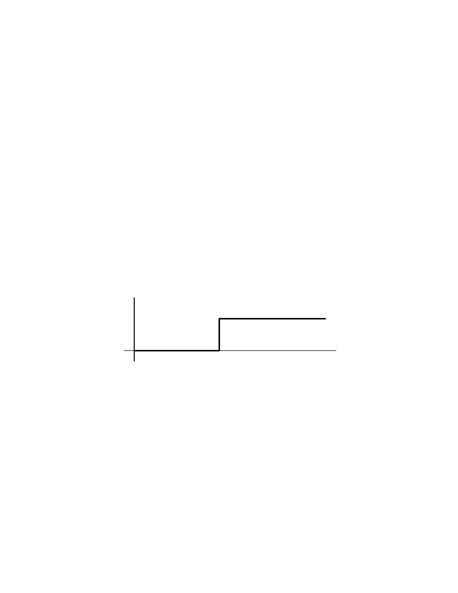
6.3: Step functions
Topics:
• Definition and basic application of unit step (Heaviside) function,
• Laplace transform of step functions and functions involving step func-
tions (piecewise continuous functions),
• Inverse transform involving step functions.
We use steps functions to form piecewise continuous functions.
Unit step function(Heaviside function):
u
c
t =
0, 0 ≤ t < c,
1, c ≤ t.
for c ≥ 0. A plot of u
c
(t) is below:
-
t
0
6
u
c
c
1
For a given function f (t), if it is multiplied with u
c
(t), then
u
c
tf (t) =
0,
0 < t < c,
f (t), c ≤ t.
We say u
c
picks up the interval [c, ∞).
Example
1. Consider
1 − u
c
(t) =
1, 0 ≤ t < c,
0, c ≤ t.
A plot of this is given below
80
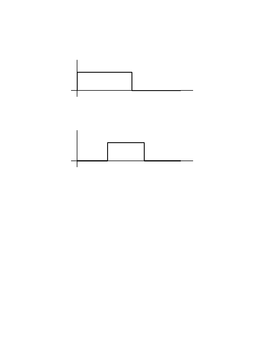
-
t
0
6
1 − u
c
c
1
We see that this function picks up the interval [0, c).
Example
2. Rectangular pulse. The plot of the function looks like
-
t
0
6
u
a
− u
b
1
a
b
for 0 ≤ a < b < ∞. We see it can be expressed as
u
a
(t) − u
b
(t)
and it picks up the interval [a, b).
Example
3. For the function
g(t) =
f (t), a ≤ t < b
0,
otherwise
We can rewrite it in terms of the unit step function as
g(t) = f (t) ·
u
a
(t) − u
b
(t)
.
Example
4. For the function
f t =
sin t, 0 ≤ t < 1,
e
t
,
1 ≤ t < 5,
t
2
5 ≤ t,
81
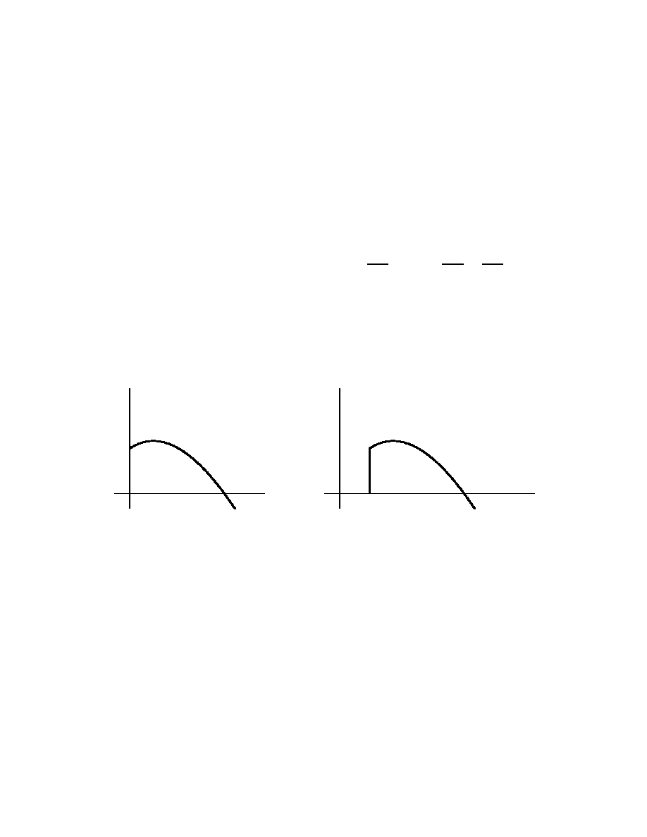
we can rewrite it in terms of the unit step function as we did in Example 3,
treat each interval separately
f (t) = sin t ·
u
0
(t) − u
1
(t)
+ e
t
·
u
1
(t) − u
5
(t)
+ t
2
· u
5
(t).
Laplace transform of
u
c
(t): by definition
L{u
c
(t)} =
Z
∞
0
e
−st
u
c
(t) dt =
Z
∞
c
e
−st
·1 dt =
e
−st
−s
∞
t=c
= 0−
e
−sc
−s
=
e
−st
s
,
(s > 0).
Shift of a function
: Given f (t), t > 0, then
g(t) =
f(t − c), c ≤ t,
0,
0 ≤ t < c,
is the shift of f by c units. See figure below.
-
t
0
6
f
-
t
0
6
g
c
Let F (s) = L{f(t)} be the Laplace transform of f(t). Then, the Laplace
transform of g(t) is
L{g(t)} = L{u
c
(t) · f(t − c)} =
Z
∞
0
e
−st
u
c
(t)f (t − c) dt =
Z
∞
c
e
−st
f (t − c) dt.
Let y = t − c, so t = y + c, and dt = dy, and we continue
L{g(t)} =
Z
∞
0
e
−s(y+c)
f (y) dy = e
−sc
Z
∞
0
e
−sy
f (y) dy = e
−cs
F (s).
So we conclude
L{u
c
(t)f (t − c)} = e
−cs
L{f(t)} = e
−cs
F (s) ,
82

which is equivalent to
L
−1
{e
−cs
F (s)} = u
c
(t)f (t − c) .
Note now we are only considering the domain t ≥ 0. So u
0
(t) = 1 for all
t ≥ 0.
In following examples we will compute Laplace transform of piecewise con-
tinuous functions with the help of the unit step function.
Example
5. Given
f (t) =
sin t,
0 ≤ t <
π
4
,
sin t + cos(t −
π
4
),
π
4
≤ t.
It can be rewritten in terms of the unit step function as
f (t) = sin t + u
π
4
(t) · cos(t −
π
4
).
(Or, if we write out each intervals
f (t) = sin t(1 − u
π
4
(t)) + (sin t + cos(t −
π
4
))u
π
4
(t) = sin t + u
π
4
(t) · cos(t −
π
4
).
which gives the same answer.)
And the Laplace transform of f is
F (s) = L{sin t} + L{u
π
4
(t) · cos(t −
π
4
)} =
1
s
2
+ 1
+ e
−
π
4
s
s
s
2
+ 1
.
Example
6. Given
f (t) =
t, 0 ≤ t < 1,
1, 1 ≤ t.
It can be rewritten in terms of the unit step function as
f (t) = t(1 − u
1
(t)) + 1 · u
1
(t) = t − (t − 1)u
1
(t) .
83

The Laplace transform is
L{f(t)} = L{t} − L{(t − 1)u
1
(t)} =
1
s
2
− e
−s
1
s
2
.
Example
7. Given
f (t) =
0,
0 ≤ t < 2,
t + 3, 2 ≤ t.
We can rewrite it in terms of the unit step function as
f (t) = (t + 3)u
2
(t) = (t − 2 + 5)u
2
(t) = (t − 2)u
2
(t) + 5u
2
(t) .
The Laplace transform is
L{f(t)} = L{(t − 2)u
2
(t)} + 5L{u
2
(t)} = e
−2s
1
s
2
+ 5e
−2s
1
s
.
Example
8. Given
g(t) =
1,
0 ≤ t < 2,
t
2
, 2 ≤ t.
We can rewrite it in terms of the unit step function as
g(t) = 1 · (1 − u
2
(t)) + t
2
u
2
(t) = 1 + (t
2
− 1)u
2
(t) .
Observe that
t
2
− 1 = (t − 2 + 2)
2
− 1 = (t − 2)
2
+ 4(t − 2) + 4 − 1 = (t − 2)
2
+ 4(t − 2) + 3 ,
we have
g(t) = 1 + (t
− 2)
2
+ 4(t − 2) + 3
u
2
(t) .
The Laplace transform is
L{g(t)} =
1
s
+ e
−2s
2
s
3
+
4
s
2
+
3
s
.
Example
9. Given
f (t) =
0,
0 ≤ t < 3,
e
t
, 3 ≤ t < 4,
0,
4 ≤ t.
84

We can rewrite it in terms of the unit step function as
f (t) = e
t
(u
3
(t) − u
4
(t)) = u
3
(t)e
t−3
e
3
− u
4
(t)e
t−4
e
4
.
The Laplace transform is
L{g(t)} = e
3
e
−3s
1
s − 1
− e
4
e
−4s
1
s − 1
=
1
s − 1
e
−3(s−1)
− e
−4(s−1)
.
Inverse transform
: We use two properties:
L{u
c
(t)} = e
−cs
1
s
,
and
L{u
c
(t)f (t − c)} = e
−cs
· L{f(t)} .
In the following examples we want to find f (t) = L
−1
{F (s)}.
Example
10.
F (s) =
1 − e
−2s
s
3
=
1
s
3
− e
−2s
1
s
3
.
We know that L
−1
{
1
s
3
} =
1
2
t
2
, so we have
f (t) = L
−1
{F (s)} =
1
2
t
2
− u
2
(t)
1
2
(t − 2)
2
=
1
2
t
2
,
0 ≤ t < 2,
1
2
t
2
−
1
2
(t − 2)
2
, 2 ≤ t.
Example
11. Given
F (s) =
e
−3s
s
2
+ s − 12
= e
−3s
1
(s + 4)(s + 3)
= e
−3s
A
s + 4
+
B
s − 3
.
By partial fraction, we find A = −
1
7
and B =
1
7
. So
f (t) = L
−1
{F (s)} = u
3
(t)
Ae
−4(t−3)
+ Be
3(t−3)
=
1
7
u
3
(t)
−e
−4(t−3)
+ e
3(t−3)
which can be written as a p/w continuous function
f (t) =
0,
0 ≤ t < 3,
−
1
7
e
−4(t−3)
+
1
7
e
3(t−3)
,
3 ≤ t.
85

Example
12. Given
F (s) =
se
−s
s
2
+ 4s + 5
= e
−s
s + 2 − 2
(s + 2)
2
+ 1
= s
−s
s + 2 − 2
(s + 2)
2
+ 1
+
s + 2 − 2
(s + 2)
2
+ 1
.
So
f (t) = L
−1
{F (s)} = u
1
(t)
e
−2(t−1)
cos(t − 1) − 2e
−2(t−1)
sin(t − 1)
which can be written as a p/w continuous function
f (t) =
0,
0 ≤ t < 1,
e
−2(t−1)
[cos(t − 1) − 2 sin(t − 1)] ,
1 ≤ t.
86

6.4: Differential equations with discontinuous
forcing functions
Topics:
• Solve initial value problems with discontinuous force, examples of var-
ious cases,
• Describe behavior of solutions, and make physical sense of them.
Next we study initial value problems with discontinuous force. We will start
with an example.
Example
1. (Damped system with force, complex roots) Solve the following
initial value problem
y
′′
+ y
′
+ y = g(t),
g(t) =
0, 0 ≤ t < 1,
1, 1 ≤ t,
,
y(0) = 1,
y
′
(0) = 0 .
Answer.
Let L{y(t)} = Y (s), so L{y
′
} = sY − 1 and L{y
′′
} = s
2
Y − s.
Also we have L{g(t)} = L{u
1
(t)} = e
−s 1
s
. Then
s
2
Y − s + sY − 1 + Y = e
−s
1
s
,
which gives
Y (s) =
e
−s
s(s
2
+ s + 1)
+
s + 1
s
2
+ s + 1
.
Now we need to find the inverse Laplace transform for Y (s). We have to do
partial fraction first. We have
1
s(s
2
+ s + 1)
=
A
s
+
Bs + C
s
2
+ s + 1
.
Compare the numerators on both sides:
1 = A(s
2
+ s + 1) + (Bs + C) · s
Set s = 0, we get A = 1.
87

Compare s
2
-term: 0 = A + B, so B = −A = −1.
Compare s-term: 0 = A + C, so C = −A = −1.
So
Y (s) = e
−s
1
s
−
s + 1
s
2
+ s + 1
+
s + 1
s
2
+ s + 1
.
We work out some detail
s + 1
s
2
+ s + 1
=
s + 1
(s +
1
2
)
2
+ (
√
3
2
)
2
=
(s +
1
2
) +
1
√
3
·
√
3
2
(s +
1
2
)
2
+ (
√
3
2
)
2
,
so
L
−1
s + 1
s
2
+ s + 1
= e
−
1
2
t
cos
√
3
2
t +
1
√
3
sin
√
3
2
t
!
.
We conclude
y(t) = u
1
(t)
"
1 − e
−
1
2
(t−1)
cos
√
3
2
(t − 1) − sin
√
3
2
(t − 1)
!#
+e
−
1
2
t
"
cos
√
3
2
t +
1
√
3
sin
√
3
2
t
#
.
Remark: There are other ways to work out the partial fractions.
Extra question: What happens when t → ∞?
Answer: We see all the terms with the exponential function will go to zero,
so y → 1 in the limit. We can view this system as the spring-mass system
with damping. Since g(t) becomes constant 1 for large t, and the particular
solution (which is also the steady state) with 1 on the right hand side is 1,
which provides the limit for y.
Further observation:
• We see that the solution to the homogeneous equation is
e
−
1
2
t
"
c
1
cos
√
3
2
t + c
2
sin
√
3
2
t
#
,
and these terms do appear in the solution.
88
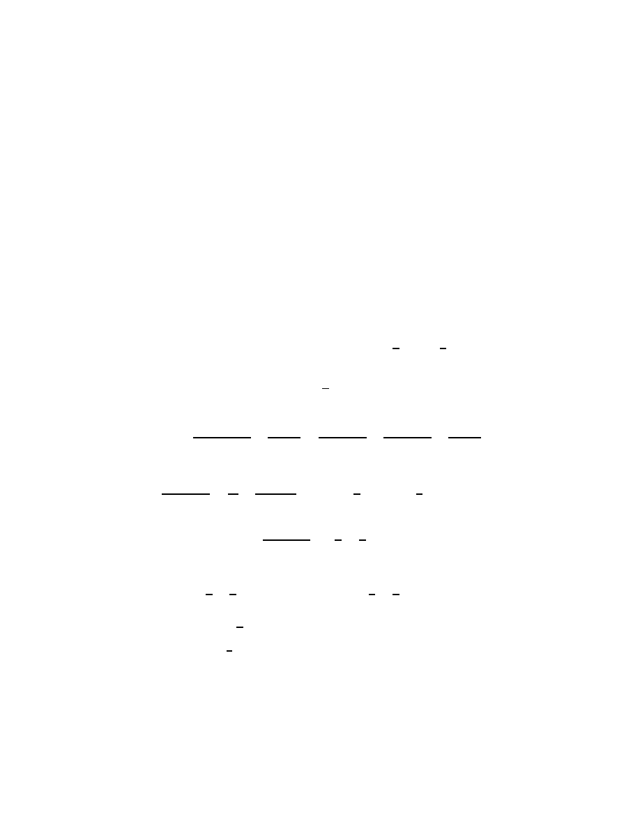
• Actually the solution consists of two part: the forced response and the
homogeneous solution.
• Furthermore, the g has a discontinuity at t = 1, and we see a jump in
the solution also for t = 1, as in the term u
1
(t).
Example
2. (Undamped system with force, pure imaginary roots) Solve the
following initial value problem
y
′′
+ 4y = g(t) =
0, 0 ≤ t < π,
1, π ≤ t < 2π,
0, 2π ≤ t,
y(0) = 1,
y
′
(0) = 0 .
Rewrite
g(t) = u
π
(t) − u
2π
(t),
L{g} = e
−πs
1
s
− e
−2π
1
s
.
So
s
2
Y − s + 4Y =
1
s
e
−π
− e
−2π
.
Solve it for Y :
Y (s) =
e
−π
− e
−2π
s(s
2
+ 4)
+
s
s
2
+ 4
=
e
−π
s(s
2
+ 4)
−
e
−2π
s(s
2
+ 4)
+
s
s
2
+ 4
.
Work out partial fraction
1
s(s
2
+ 4)
=
A
s
+
Bs + C
s
2
+ 4
,
A =
1
4
,
B = −
1
4
,
C = 0.
So
L
−1
{
1
s(s
2
+ 4)
} =
1
4
−
1
4
cos 2t .
Now we take inverse Laplace transform of Y
y(t) = u
π
(t)
1
4
−
1
4
cos 2(t − π)
− u
2π
(t)
1
4
−
1
4
cos 2(t − 2π)
+ cos 2t
= (u
π
(t) − u
2π
)
1
4
(1 − cos 2t) + cos 2t
= cos 2t +
(
1
4
(1 − cos 2t), π ≤ t < 2π,
0,
otherwise,
= homogeneous solution + forced response
89

Example
3. In Example 2, let
g(t) =
0,
0 ≤ t < 4,
e
t
, 4 ≤ 5 < 2π,
0,
5 ≤ t.
Find Y (s).
Answer.
Rewrite
g(t) = e
t
(u
4
(t) − u
5
(t)) = u
4
(t)e
t−4
e
4
− u
5
(t)e
t−5
e
5
,
so
G(s) = L{g(t)} = e
4
e
−4s
1
s − 1
− e
5
e
−5s
1
s − 1
.
Take Laplace transform of the equation, we get
(s
2
+4)Y (s) = G(s)+s,
Y (s) = e
4
e
−4s
− e
5
e
−5s
1
(s − 1)(s
2
+ 4)
+
s
s
2
+ 4
.
Remark: We see that the first term will give the forced response, and the
second term is from the homogeneous equation.
The students may work out the inverse transform as a practice.
Example
4. (Undamped system with force, example 2 from the book p.
334)
y
′′
+ 4y = g(t),
y(0) = 0, y
′
(0) = 0,
g(t) =
0,
0 ≤ t < 5,
(t − 5)/5, 5 ≤ 5 < 10,
1,
10 ≤ t.
Let’s first work on g(t) and its Laplace transform
g(t) =
t − 5
5
(u
5
(t) − u
10
(t)) + u
10
(t) =
1
5
u
5
(t)(t − 5) −
1
5
u
10
(t)(t − 10),
G(s) = L{g} =
1
5
e
−5s
1
s
2
−
1
5
e
−10s
1
s
2
Let Y (s) = L{y}, then
(s
2
+4)Y (s) = G(s),
Y (s) =
G(s)
s
2
+ 4
=
1
5
e
−5s
1
s
2
(s
2
+ 4)
−
1
5
e
−10s
1
s
2
(s
2
+ 4)
90

Work out the partial fraction:
H(s)
.
=
1
s
2
(s
2
+ 4)
=
A
s
+
B
s
2
+
Cs + 2D
s
2
+ 4
one gets A = 0, B =
1
4
, C = 0, D = −
1
8
. So
h(t)
.
= L
−1
1
s
2
(s
2
+ 4)
= L
−1
1
4
·
1
s
2
−
1
8
·
2
s
2
+ 2
2
=
1
4
t −
1
8
sin 2t.
Go back to y(t)
y(t) = L
−1
{Y } =
1
5
u
5
(t)h(t − 5) −
1
5
u
10
(t)h(t − 10)
=
1
5
u
5
(t)
1
4
(t − 5) −
1
8
sin 2(t − 5)
−
1
5
u
10
(t)
1
4
(t − 10) −
1
8
sin 2(t − 10)
=
0,
0 ≤ t < 5,
1
20
(t − 5) −
1
40
sin 2(t − 5),
5 ≤ 5 < 10,
1
4
−
1
40
(sin 2(t − 5) − sin 2(t − 10)), 10 ≤ t.
Note that for t ≥ 10, we have y(t) =
1
4
+ R · cos(2t + δ) for some amplitude
R and phase δ.
The plots of g and y are given in the book. Physical meaning and qualitative
nature of the solution:
The source g(t) is known as ramp loading. During the interval 0 < t < 5,
g = 0 and initial conditions are all 0. So solution remains 0. For large time
t, g = 1. A particular solution is Y =
1
4
. Adding the homogeneous solution,
we should have y =
1
4
+ c
1
sin 2t + c
2
cos 2t for t large. We see this is actually
the case, the solution is an oscillation around the constant
1
4
for large t.
91

Chapter 7. Systems of two linear differential
equations
7.1: Introduction to systems of differential equa-
tions
Given
ay
′′
+ by
′
+ cy = g(t),
y(0) = α,
y
′
(0) = β
we can do a variable change: let
x
1
= y,
x
2
= x
′
1
= y
′
then
(
x
′
1
= x
2
x
′
2
= y
′′
=
1
a
(g(t) − bx
2
− cx
1
)
x
1
(0) = α
x
2
(0) = β
Observation: For any 2nd order equation, we can rewrite it into a system of
2 first order equations.
Example
1. Given
y
′′
+ 5y
′
− 10y = sin t,
y(0) = 2,
y
′
(0) = 4
Rewrite it into a system of first order equations: let x
1
= y and x
2
= y
′
= x
′
1
,
then
x
′
1
= x
2
x
′
2
= y
′′
= −5x
2
+ 10x
1
+ sin t
I.C.’s:
x
1
(0) = 2
x
2
(0) = 4
We can do the same thing to any high order equations. For n-th order
differential equation:
y
(n)
= F (t, y, y
′
, · · · , y
(n−1)
)
define the variable change:
x
1
= y,
x
2
= y
′
,
· · · x
n
= y
(n−1)
92

we get
x
′
1
= y
′
= x
2
x
′
2
= y
′′
= x
3
...
x
′
n−1
= y
(n−1)
= x
n
x
′
n
= y
(n)
= F (t, x
1
, x
2
, · · · , x
n
)
with corresponding source terms.
Reversely, we can convert a 1st order system into a high order equation.
Example
2. Given
x
′
1
= 3x
1
− 2x
2
x
′
2
= 2x
1
− 2x
2
x
1
(0) = 3
x
2
(0) =
1
2
Eliminate x
2
: the first equation gives
2x
2
= 3x
1
− x
′
1
,
x
2
=
3
2
x
1
−
1
2
x
′
1
.
Plug this into second equation, we get
3
2
x
1
−
1
2
x
′
1
′
= 2x
1
− 2x
2
= −x
1
+ x
′
1
3
2
x
′
1
−
1
2
x
′′
1
= −x
1
+ x
′
1
x
′′
1
− x
′
1
− 2x
1
= 0
with the initial conditions:
x
1
(0) = 3,
x
′
1
(0) = 3x
1
(0) − 2x
2
(0) = 8.
This we know how to solve!
Definition of a solution: a set of functions x
1
(t), x
2
(t), · · · , x
n
(t) that satisfy
the differential equations and the initial conditions.
93

7.2: Review of matrices
A matrix of size m × n:
A =
a
1,1
· · · a
1,n
...
a
m,1
· · · a
m,n
= (a
i,j
),
1 ≤ i ≤ m, 1 ≤ j ≤ n.
We consider only square matrices, i.e., m = n, in particular for n = 2 and 3.
Basic operations: A, B are two square matrices of size n.
• Addition: A + B = (a
ij
) + (b
ij
) = (a
ij
+ b
ij
)
• Scalar multiple: αA = (α · a
ij
)
• Transpose: A
T
switch the a
i,j
with a
ji
. (A
T
)
T
= A.
• Product: For A · B = C, it means c
i,j
is the inner product of (ith row
of A) and (jth column of B). Example:
a b
c d
·
x y
u v
=
ax + bu ay + bv
cx + du cy + dv
We can express system of linear equations using matrix product.
Example
1.
x
1
− x
2
+ 3x
3
= 4
2x
1
+ 5x
3
= 0
x
2
− x
3
= 7
can be expressed as:
1 −1
3
2
0
5
0
1
−1
·
x
1
x
2
x
3
=
4
0
7
Example
2.
x
′
1
= a(t)x
1
+ b(t)x
2
+ g
1
(t)
x
′
2
= c(t)x
1
+ d(t)x
2
+ g
2
(t)
⇒
x
1
x
2
′
=
a(t) b(t)
c(t) d(t)
·
x
1
x
2
+
g
1
(t)
g
2
(t)
Some properties:
• Identity I: I = diag(1, 1, · · · , 1), AI = IA = A.
94

• Determinant det(A):
det
a b
c d
= ad − bc,
det
a b
c
u v w
x y z
= avx + bwx + cuy − xvc − ywa − zub.
• Inverse inv(A) = A
−1
: A
−1
A = AA
−1
= I.
• The following statements are all equivalent:
–
(1) A is invertible;
–
(2) A is non-singular;
–
(3) det(A) 6= 0;
–
(4) row vectors in A are linearly independent;
–
(5) column vectors in A are linearly independent.
–
(6) All eigenvalues of A are non-zero.
95

7.3: Eigenvalues and eigenvectors
Eigenvalues and eigenvectors of
A (A is 2 × 2 or 3 × 3.)
λ: scalar value,
~v: column vector, ~v 6≡ 0.
If A~v = λ~v, then (λ, ~v) is the (eigenvalue, eigenvector) of A.
They are also called an eigen-pair of A.
Remark: If ~v is an eigenvector, then α~v for any α 6= 0 is also an eigenvector,
because
A(α~v) = αA~v = αλ~v = λ(α~v).
How to find (λ, v):
A~v − λ~v = 0,
(A − λI)~v = 0,
det(A − λI) = 0.
We see that det(A − λI) is a polynomial of degree 2 (or 3) in λ, and it is also
called the characteristic polynomial of A. We need to find its roots.
Example
1: Find the eigenvalues and the eigenvectors of A where
A =
1 1
4 1
.
Answer.
Let’s first find the eigenvalues.
det(A−λI) = det
1 − λ
1
4
1 − λ
= (1−λ)
2
−4 = 0,
λ
1
= −1, λ
2
= 3.
Now, let’s find the eigenvector ~v
1
for λ
1
= −1: let ~v
1
= (a, b)
T
(A − λ
1
I)~v
1
= 0,
⇒
1 − (−1)
1
4
1 − (−1)
·
a
b
=
0
0
,
⇒
2 1
4 2
·
a
b
=
0
0
,
so
2a + b = 0,
choose a = 1, then we have b = −2,
⇒
~v
1
=
1
−2
.
96

Finally, we will compute the eigenvector ~v
2
= (c, d)
T
for λ
2
= 3:
(A − λ
1
I)~v
2
= 0,
⇒
1 − 3
1
4
1 − 3
·
c
d
=
0
0
,
⇒
−2 1
4
−2
·
c
d
=
0
0
,
so
2c − d = 0,
choosec = 1, then we have d = 2,
⇒
~v
2
=
1
2
.
Example
2. Eigenvalues can be complex numbers.
A =
2 −9
4
2
.
Let’s first find the eigenvalues.
det(A−λI) = det
2 − λ
−9
4
2 − λ
= (2 −λ)
2
+ 36 = 0,
⇒
λ
1,2
= 2 ±6i
We see that λ
2
= ¯
λ
1
, complex conjugate. The same will happen to the
eigenvectors, i.e., ~v
1
= ¯
~v
2
. So we need to only find one. Take λ
1
= 2 + 6i, we
compute ~v = (v
1
, v
2
)
T
:
(A − λ
1
I)~v = 0,
−i6 −9
4
−i6
·
v
1
v
2
= 0,
−6iv
1
− 9v
2
= 0,
choose v
1
= 1, so v
2
= −
2
3
i,
so
~v
1
=
1
−
2
3
i
,
~v
2
= ¯
~v
1
=
1
2
3
i
.
97

7.4: Basic theory of systems of first order lin-
ear equation
General form of a system of first order equations written in matrix-vector
form:
~x
′
= P (t)~x + ~g.
If ~g = 0, it is homogeneous. We only consider this case, so
~x
′
= P (t)~x.
Superposition
: If ~x
1
(t) and ~x
2
(t) are two solutions of the homogeneous
system, then any linear combination c
1
~x
1
+ c
2
~x
2
is also a solution.
Wronskian
of vector-valued functions are defined as
W [~x
1
(t), ~x
2
(t), · · · , ~x
n
(t)] = det X(t)
where X is a matrix whose columns are the vectors ~x
1
(t), ~x
2
(t), · · · , ~x
n
(t).
If det X(t) 6= 0, then ~x
1
(t), ~x
2
(t), · · · , ~x
n
(t)
is a set of linearly independent
functions.
A set of linearly independent solutions ~x
1
(t), ~x
2
(t), · · · , ~x
n
(t)
is said to be
a fundamental set of solutions.
The general solution is the linear combination of these solutions, i.e.
~x = c
1
~x
1
(t) + c
2
~x
2
(t) + · · · + c
n
~x
n
(t).
98

7.5: Homogeneous systems of two equations
with constant coefficients.
We consider the following initial value problem:
x
′
1
= ax
1
+ bx
2
x
′
2
= cx
1
+ dx
2
I.C.’s:
x
1
(0) = ¯
x
1
x
2
(0) = ¯
x
2
In matrix vector form:
~x
′
= A~x,
~x =
x
1
x
2
,
~x(0) =
¯
x
1
¯
x
2
A =
a b
c d
.
Claim
: If (λ, ~v) is an eigen-pair for A, then ~z = e
λt
~v is a solution to ~x
′
= A~x.
Proof.
~z
′
= (e
λt
~v)
′
= (e
λt
)
′
~v = λe
λt
~v
A~z = A(e
λt
~v) = e
λt
(A~v) = e
λt
λ~v
Therefore ~z
′
= A~z so ~z is a solution.
Steps to solve the initial value problem:
• Step I: Find eigenvalues of A: λ
1
, λ
2
.
• Step II: Find the corresponding eigenvectors ~v
1
, ~v
2
.
• Step III: Form two solutions: ~z
1
= e
λ
1
t
~v
1
, ~z
2
= e
λ
2
t
~v
2
.
• Step IV: Check that ~z
1
, ~z
2
are linearly independent: the Wronskian
W (~z
1
, ~z
2
) = det(~z
1
, ~z
2
) 6= 0.
(This step is usually OK in our problems.)
• Step V: Form the general solution: ~x = c
1
~z
1
+ c
2
~z
2
.
• If initial condition ~x(0) is given, then use it to determine c
1
, c
2
.
99

We will start with an example.
Example
1. Solve
~x
′
= A~x,
A =
1 1
4 1
.
First, find out the eigenvalues of A. By an example in 7.3, we have
λ
1
= −1,
λ
2
= 3,
~v
1
=
1
−2
,
~v
1
=
1
2
,
So the general solution is
~x = c
1
e
λ
1
t
~v
1
+ c
2
e
λ
2
t
~v
2
= c
1
e
−t
1
−2
+ c
2
e
3t
1
2
.
Write it out in components:
x
1
(t) = c
1
e
−t
+ c
2
e
3t
x
2
(t) = −2c
1
e
−t
+ 2c
2
e
3t
.
Qualitative property of the solutions:
• What happens when t → ∞?
If c
2
> 0, then x
1
→ ∞, x
2
→ ∞.
If c
2
< 0, then x
1
→ −∞, x
2
→ −∞.
Asymptotic relation between x
1
, x
2
: look at
x
1
x
2
:
x
1
x
2
=
c
1
e
−t
+ c
2
e
3t
−2c
1
e
−t
+ 2c
2
e
3t
.
As t → ∞, we have
x
1
x
2
=
c
2
e
3t
2c
2
e
3t
=
1
2
.
This means, x
1
→ 2x
2
asymptotically.
• What happens when t → −∞?
Looking at
x
1
x
2
, we see as t → −∞ we have
x
1
x
2
=
c
1
e
−t
−2c
1
e
−t
= −
1
2
,
which means, x
1
→ −2x
2
asymptotically as t → −∞.
100
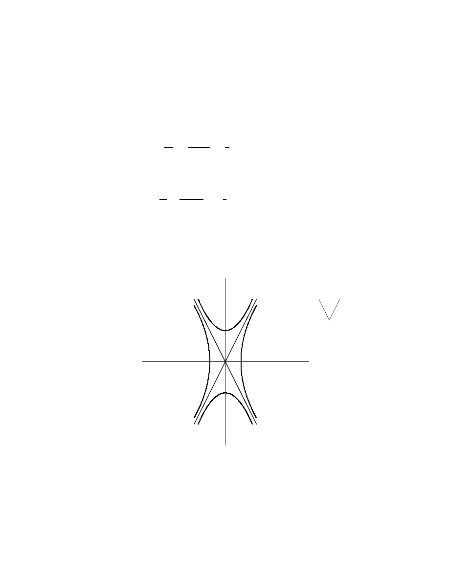
Phase portrait.
is the trajectories of various solutions in the x
2
− x
1
plane.
• Since A is non-singular, then ~x = ~0 is the only critical point such that
~x
′
= A~x = 0.
• If c
1
= 0, then
x
1
x
2
=
c
2
e
3t
2c
2
e
3t
=
1
2
, so the trajectory is a straight line
x
1
= 2x
2
.
Note that this is exactly the direction of ~v
2
.
Since λ
2
= 3 > 0, the trajectory is going away from 0.
• If c
2
= 0, then
x
1
x
2
=
c
1
e
−
t
−2c
1
e
−
t
= −
1
2
, so the trajectory is another straight
line x
1
= −2x
2
.
Note that this is exactly the direction of ~v
1
.
Since λ
2
= −1 < 0, the trajectory is going towards 0.
• For general cases where c
1
, c
2
are not 0, the trajectories should start
(asymptotically) from line x
1
= −2x
2
, and goes to line x
1
= 2x
2
asymp-
totically as t grows.
-
x
1
6
x
2
K
~v
2
~v
1
U
K
~v
1
~v
2
-
?
6
Definition:
If A has two real eigenvalues of opposite signs, the origin (critical
point) is called a saddle point. A saddle point is unstable.
Tips for drawing phase portrait for saddle point: only need the eigenvalues
and eigenvectors!
101

General case: If two eigenvalues of A are λ
1
< 0 and λ
2
> 0, with two
corresponding eigenvectors ~v
1
, ~v
2
. To draw the phase portrait, we follow
these guidelines:
• The general solution is
~x = c
1
e
λ
1
t
~v
1
+ c
2
e
λ
2
t
~v
2
.
• If c
1
= 0, then the solution is ~x = c
2
e
λ
2
t
~v
2
. We see that the solution
vector is a scalar multiple of ~v
2
. This means a line parallel to ~v
2
through
the origin is a trajectory. Since λ
2
> 0, solutions |~x| → ∞ along this
line, so the arrows are pointing away from the origin.
• The similar other half: if c
2
= 0, then the solution is ~x = c
1
e
λ
1
t
~v
1
.
We see that the solution vector is a scalar multiple of ~v
1
. This means
a line parallel to ~v
1
through the origin is a trajectory. Since λ
1
< 0,
solutions approach 0 along this line, so the arrows are pointing toward
the origin.
• Now these two lines cut the plane into 4 regions. We need to draw at
least one trajectory in each region. In the region, we have the general
case, i.e., c
1
6= 0 and c
2
6= 0. We need to know the asymptotic behavior.
We have
t → ∞, => ~x → c
2
e
λ
2
t
~v
2
t → −∞, => ~x → c
1
e
λ
1
t
~v
1
We see these are exactly the two straight lines we just made. This
means, all trajectories come from the direction of ~v
1
, and will approach
~v
2
as t grows. See the plot below.
102
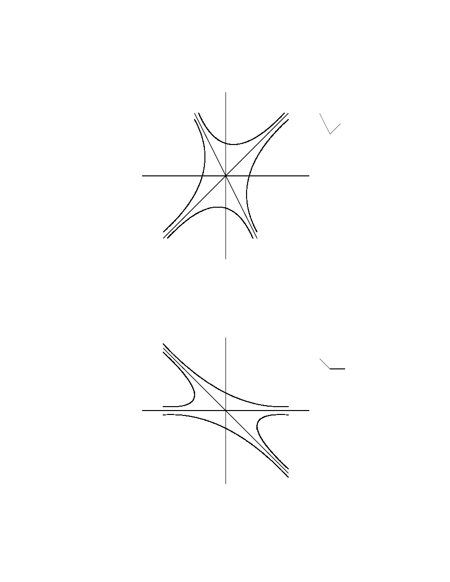
-
x
1
6
x
2
K
~v
2
~v
1
U
K
~v
1
~v
2
i
q
Example
2. Suppose we know the eigenvalues and eigenvectors of A:
λ
1
= 3,
~v
1
=
1
−1
,
λ
1
= −3,
~v
2
=
1
0
.
Then the phase portrait looks like this:
-
x
1
6
x
2
-
I
~v
2
~v
1
-
I
R
~v
1
~v
2
6
?
j
Y
103

If the two real distinct eigenvalue have the same sign, the situation is quite
different.
Example
3. Consider the homogeneous system
~x
′
= A~x,
A =
−3 2
1
−2
.
Find the general solution and sketch the phase portrait.
Answer.
• Eigenvalues of A:
det(A−λI) = det
−3 2
1
−2
= (−3−λ)(−2−λ)−2 = λ
2
+5λ+4 = (λ+1)(λ+4) = 0,
So λ
1
= −1, λ
2
= −4. (Two eigenvalues are both negative!)
• Find the eigenvector for λ
1
. Call it ~v
1
= (a, b)
T
,
(A−λ
1
I)~v
1
=
−3 + 1
2
1
−2 + 1
·
a
b
=
−2 2
1
−1
·
a
b
=
0
0
.
This gives a = b. Choose it to be 1, we get ~v
1
= (1, 1)
T
.
• Find the eigenvector for λ
2
. Call it ~v
2
= (c, d)
T
,
(A−λ
2
I)~v
1
=
−3 + 4
2
1
−2 + 4
·
c
d
=
1 2
1 2
·
c
d
=
0
0
.
This gives c + 2d = 0. Choose d = 1, then c = −2. So ~v
2
= (−2, 1)
T
.
• General solution is
~x(t) = c
1
e
λ
1
t
~v
1
+ c
2
e
λ
2
t
~v
2
= c
1
e
−t
1
1
+ c
2
e
−4t
−2
1
.
Write it out in components:
x
1
(t) = c
1
e
−t
− 2c
2
e
−4t
x
2
(t) = c
1
e
−t
+ c
2
e
−4t
.
104
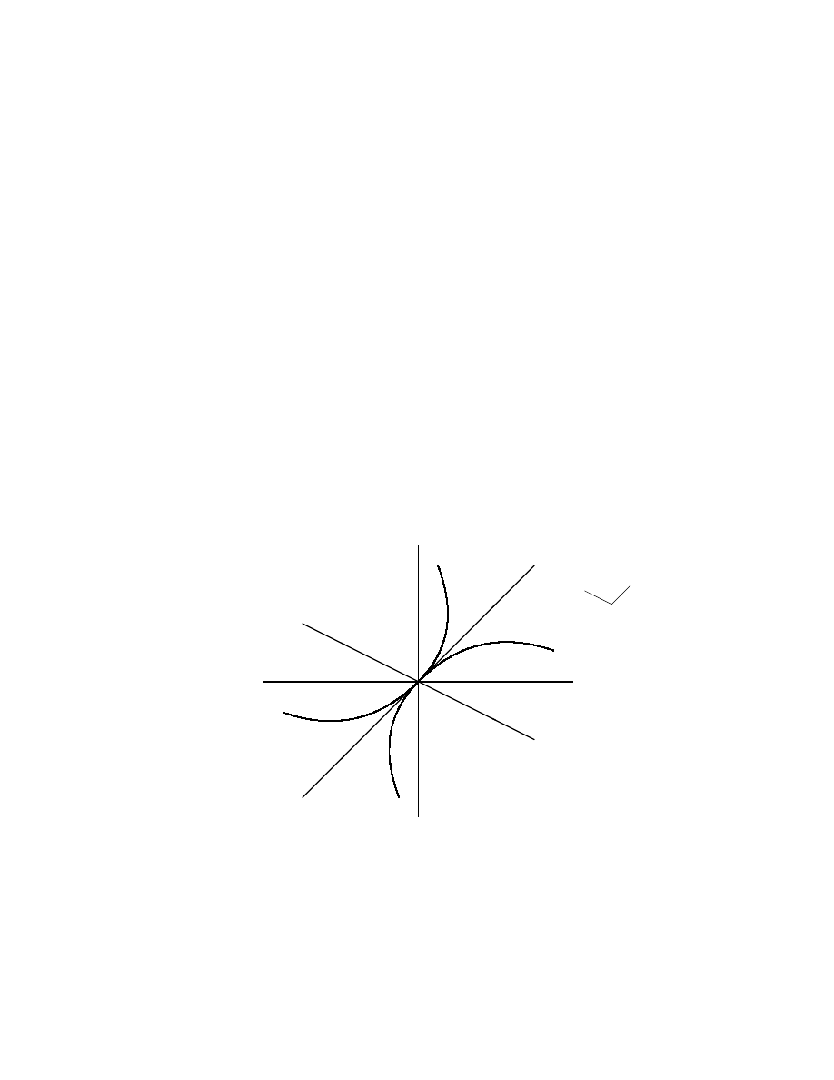
Phase portrait:
• If c
1
= 0, then ~x = c
2
e
λ
2
t
~v
2
, so the straight line through the origin
in the direction of ~v
2
is a trajectory. Since λ
2
< 0, the arrows point
toward the origin.
• If c
2
= 0, then ~x = c
1
e
λ
1
t
~v
1
, so the straight line through the origin
in the direction of ~v
1
is a trajectory. Since λ
1
< 0, the arrows point
toward the origin.
• For the general case, when c
1
6= 0 and c
2
6= 0, we have
t → −∞, =>
~x → 0,
~x → c
2
e
λ
2
t
~v
2
t → ∞, =>
|~x| → ∞,
~x → c
1
e
λ
1
t
~v
1
So all trajectories come into the picture in the direction of ~v
2
, and
approach the origin in the direction of ~v
1
. See the plot below.
-
x
1
6
x
2
Y
~v
1
~v
2
j
Y
~v
1
~v
2
-
?
6
In the previous example, if λ
1
> 0, λ
2
> 0, say λ
1
= 1 and λ
2
= 4, and ~v
1
, ~v
2
are the same, then the phase portrait will look the same, but with all arrows
going away from 0.
105
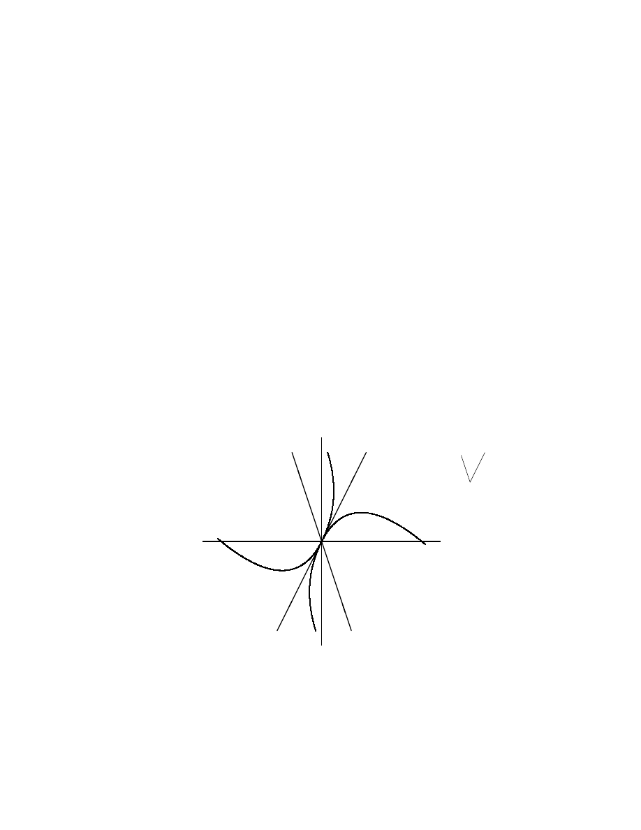
Definition:
If λ
1
6= λ
2
are real with the same sign, the critical point ~x = 0
is called a node.
If λ
1
> 0, λ
2
> 0, this node is called a source.
If λ
1
< 0, λ
2
< 0, this node is called a sink.
A sink is stable, and a source is unstable.
Example
4. (Source node) Suppose we know the eigenvalues and eigenvec-
tors of A are
λ
1
= 3,
λ
2
= 4,
~v
1
=
1
2
,
~v
2
=
1
−3
.
(1) Find the general solution for ~x
′
= A~x, (2) Sketch the phase portrait.
Answer.
(1) The general solution is simple, just use the formula
~x = c
1
e
λ
1
t
~v
1
+ c
2
e
λ
2
t
~v
2
= c
1
e
3t
1
2
+ c
2
e
4t
1
−3
.
(2) Phase portrait: Since λ
2
> λ
1
, then the solution approach ~v
2
as time
grows. As t → −∞, ~x → c
1
e
λ
1
t
~v
1
. See the plot below.
-
x
1
6
x
2
M
~v
1
~v
2
M
N
~v
1
~v
2
-
6
?
Summary:
(1). If λ
1
and λ
2
are real and with opposite sign: the origin is a saddle point,
106

and it’s unstable;
(2). If λ
1
and λ
2
are real and with same sign: the origin is a node.
If λ
1
, λ
2
> 0, it’s a source node, and it’s unstable;
If λ
1
, λ
2
< 0, it’s a sink node, and it’s stable;
107

7.6: Complex eigenvalues
If A has two complex eigenvalues, they will be a pair of complex conjugate
numbers, say λ
1,2
= α ± iβ, β 6= 0.
The two corresponding eigenvectors will also be complex conjugate, i.e,
~v
1
=¯
~v
2
.
We have two solutions
~z
1
= e
λ
1
t
~v
1
,
~z
2
= e
λ
2
t
~v
2
.
They are complex-valued functions, and they also are complex conjugate.
We seek real-valued solutions. By the principle of superposition,
~y
1
=
1
2
(~z
1
+ ~z
2
) = Re(~z
1
),
~y
2
=
1
2i
(~z
1
− ~z
2
) = Im(~z
1
)
are also two solutions, and they are real-valued.
One can show that they are linearly independent, so they form a set of
fundamental solutions. The general solution is then ~x = c
1
~y
1
+ c
2
~y
2
.
Now let’s derive the formula for the general solution. We have two eigenval-
ues: λ and ¯
λ, two eigenvectors: ~v and ¯
~v, which we can write
λ = α + iβ,
~v = ~v
r
+ i~v
i
.
One solution can be written
~z = e
λt
~v = e
(α+iβ)t
(~v
r
+ i~v
i
)e
αt
(cos βt + i sin βt) · (~v
r
+ i~v
i
)
= e
αt
(cos βt · ~v
r
− sin βt · ~v
i
+ i(sin βt · ~v
r
+ cos βt · ~v
i
)) .
The general solution is
~x = c
1
e
αt
(cos βt · ~v
r
− sin βt · ~v
i
) + c
2
e
αt
(sin βt · ~v
r
+ cos βt · ~v
i
) .
Notice now if α = 0, i.e., we have pure imaginary eigenvalues. The ~x is a
harmonic oscillation, which is a periodic function. This means in the phase
portrait all trajectories are closed curves.
108

Example
1. (pure imaginary eigenvalues.) Find the general solution and
sketch the phase portrait of the system:
~x
′
= A~x,
A =
0 −4
1
0
.
Answer.
First find the eigenvalues of A:
det(A − λI) = λ
2
+ 4 = 0,
λ
1,2
= ±2i.
Eigenvectors: need to find one ~v = (a, b)
T
for λ = 2i:
(A − λI)~v = 0,
−2i −4
1
−2i
·
a
b
=
0
0
.
a − 2ib = 0,
choose b = 1, then a = 2i,
then
~v =
2i
1
=
0
1
+ i
2
0
.
The general solution is
~x = c
1
cos 2t ·
0
1
− sin 2t ·
2
0
+c
2
sin 2t ·
0
1
+ cos 2t ·
2
0
.
Write out the components, we get
x
1
(t) = −2c
1
sin 2t + 2c
2
cos 2t
x
2
(t) = c
1
cos 2t + c
2
sin 2t.
Phase portrait:
• ~x is a periodic function, so all trajectories are closed curves around the
origin.
• They do not intersect with each other. This follows from the uniqueness
of the solution.
• They are ellipses. Because we have the relation:
(x
1
/2)
2
+ (x
2
)
2
= constant.
109

• The arrows are pointing either clockwise or counter clockwise, deter-
mined by A. In this example, take ~x = (1, 0)
T
, a point on the x
1
-axis.
By the differential equations, we get ~x
′
= A~x = (0, 1)
T
, which is a
vector pointing upward. So the arrows are counter-clockwise.
See plot below.
x
1
x
2
Definition
. The origin in this case is called a center. A center is stable
(b/c solutions don’t blow up), but is not asymptotically stable (b/c solutions
don’t approach the origin as time goes).
If the complex eigenvalues have non-zero real part, the situation is still dif-
ferent.
Example
2. Consider the system
~x
′
= A~x,
A =
3 −2
4 −1
.
First, we compute the eigenvalues:
det(A − λI) = (3 − λ)(−1 − λ) + 8 = λ
2
− 2λ + 5 = 0,
λ
1,2
= 1 ± 2i,
⇒
α = 1,
β = 2.
Eigenvectors: need to compute only one ~v = (a, b)
T
. Take λ = 1 + 2i,
(A − λI)~v =
2 − 2i
−2
4
−2 − 2i
·
a
b
=
0
0
,
110

(2 − 2i)a − 2b = 0.
Choosing a = 1, then b = 1 − i, so
~v =
1
1 − i
=
1
1
+ i
0
−1
.
So the general solution is:
~x = c
1
e
t
cos 2t ·
1
1
− sin 2t ·
0
−1
+ c
2
e
t
sin 2t ·
1
1
− cos 2t ·
0
−1
= c
1
e
t
cos 2t
cos 2t + sin 2t
+ c
2
e
t
sin 2t
sin 2t − cos 2t
.
Phase portrait.
Solution is growing oscillation due to the e
t
. If this term
is not present, (i.e., the eigenvalues would be pure imaginary), then the
solutions are perfect oscillations, whose trajectory would be closed curves
around origin, as the center. But with the e
t
term, we will get spiral curves.
Since α = 1 > 0, all arrows are pointing away from the origin.
To determine the direction of rotation, we need to go back to the original
equation and take a look at the directional field.
Consider the point (x
1
= 1, x
2
= 0), then ~x
′
= A~x = (3, 4)
T
. The arrow
should point up with slope 4/3.
At the point ~x = (0, 1)
T
, we have ~x
′
= (−2, −1)
T
.
Therefore, the spirals are rotating counter clockwise. We don’t stress on the
exact shape of the spirals. See plot below.
111
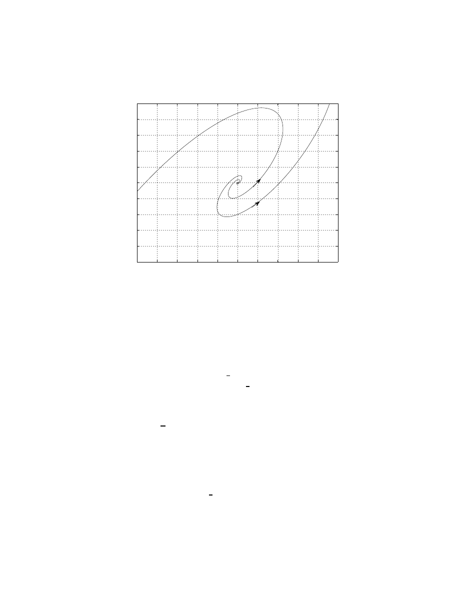
−2.5
−2
−1.5
−1
−0.5
0
0.5
1
1.5
2
2.5
−2.5
−2
−1.5
−1
−0.5
0
0.5
1
1.5
2
2.5
x
1
x
2
In this case, the origin (the critical point) is called the spiral point. The
origin in this example is an unstable critical point since α > 0.
Remark:
If α < 0, then all arrows will go towards the origin. The origin
will be a stable critical point. An example is provided in the text book. We
will go through it here.
Example
3. Consider
~x
′
=
−
1
2
1
−1 −
1
2
~x.
The eigenvalues and eigenvectors are:
λ
1,2
= −
1
2
± i,
~v =
1
±i
=
1
0
± i
0
1
.
Since the formula for the general solution is not so “friendly” to memorize,
we use a different approach.
We know that one solution is
~z = e
λ
1
t
~v
1
= e
−(
1
2
+i)t
1
0
± i
0
01
.
112

This is a complex values function. We know the real part and the imaginary
part are both solutions, so work them out:
~z = e
−
1
2
t
cos t
1
0
− sin t
0
1
+ i sin t
1
0
+ i cos t
0
1
.
The general solution is:
~x = c
1
e
−
1
2
t
cos t
1
0
− sin t
0
1
+ c
2
e
−
1
2
t
sin t
1
0
+ cos t
0
1
,
and we can write out each component
x
1
(t) = e
−
1
2
t
(c
1
cos t + c
2
sin t)
x
2
(t) = e
−
1
2
t
(−c
1
sin t + c
2
cos t)
Phase portrait: If c
1
= 0, we have
x
2
1
+ x
2
2
= (e
−
1
2
t
)
2
c
2
2
(sin
2
t + cos
2
t) = (e
−
1
2
t
)
2
c
2
2
.
If c
2
= 0, we have
x
2
1
+ x
2
2
= (e
−
1
2
t
)
2
c
2
1
.
In general, if c
1
6= 0 and c
2
6= 0, we can show:
x
2
1
+ x
2
2
= (e
−
1
2
t
)
2
(c
2
1
+ c
2
1
).
The trajectories will be spirals, with arrows pointing toward the origin. To
determine with direction they rotate, we check a point on the x
1
axis:
~x =
1
0
,
~x
′
= A~x =
−
1
2
−1
.
So the spirals rotate clockwise. And the origin is a stable equilibrium point.
See the picture below.
113
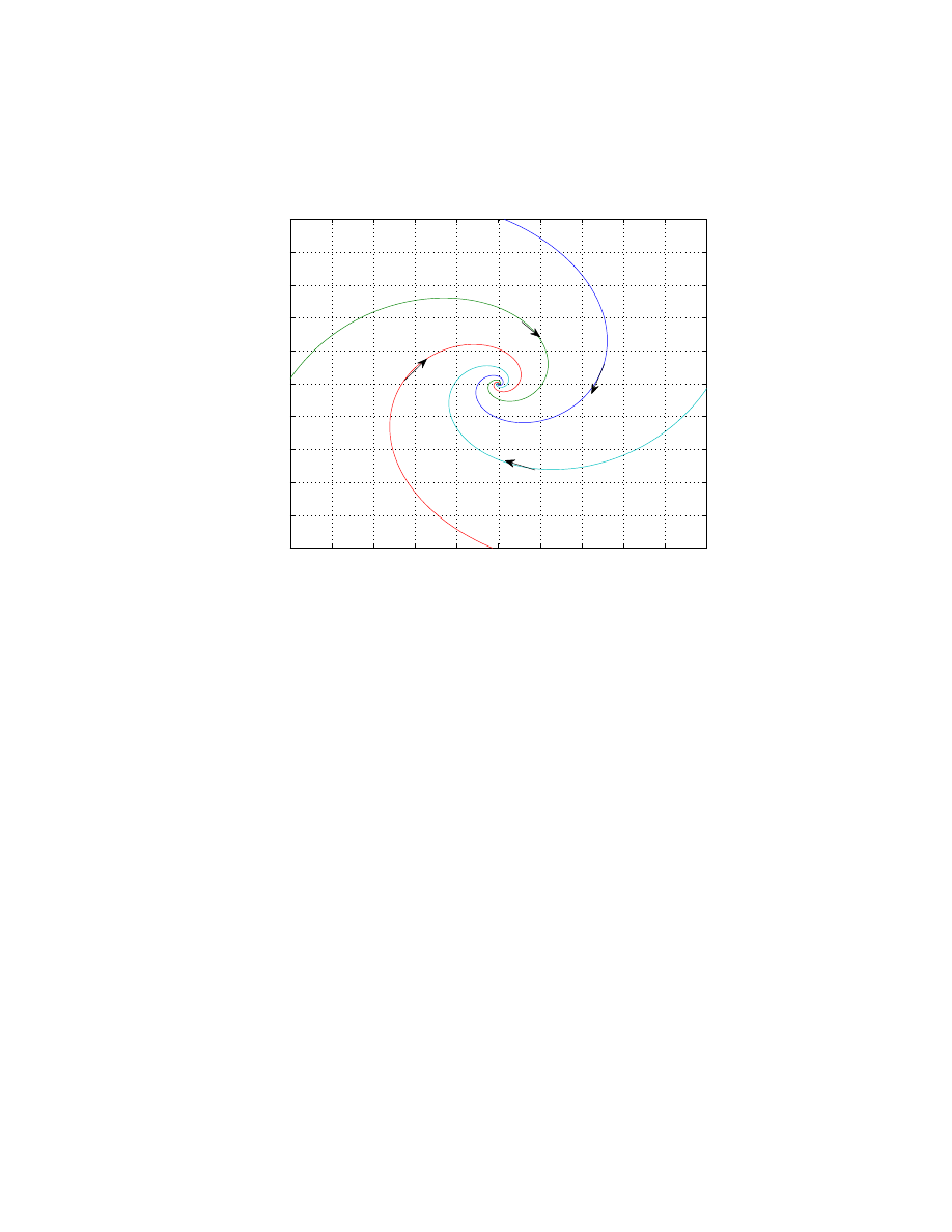
−50
−40
−30
−20
−10
0
10
20
30
40
50
−50
−40
−30
−20
−10
0
10
20
30
40
50
114

7.8: Repeated eigenvalues
Here we study the case where the two eigenvalues are the same, say λ
1
=
λ
2
= λ. This can happen, as we will see through our first example.
Example
1. Let
A =
1 −1
1
3
.
Then
det(A−λI) = det
1 − λ
−1
1
3 − λ
= (1−λ)(3−λ)+1 = λ
2
−4λ+3+1 = (λ−2)
2
= 0,
so λ
1
= λ
2
= 2. And we can find only one eigenvector ~v = (a, b)
T
(A − λI)~v =
−1 −1
1
1
·
a
b
= 0,
a + b = 0.
Choosing a = 1, then b = −1, and we find ~v =
1
−1
. Then, one solution
is:
~z
1
= e
λt
~v = e
2t
1
−1
.
We need to find a second solution. Let’s try ~z
2
= te
λt
~v. We have
~z
′
= e
λt
~v + λte
λt
~v = (1 + λt)e
λt
~v
A~z
2
= Ate
λt
~v = te
λt
(A~v) = te
λt
λ~v = λte
λt
~v
If ~z
2
is a solution, we must have
~z
′
= A~z
→
1 + λt = λt
which doesn’t work.
Try something else: ~z
2
= te
λt
~v + ~ηe
λt
. (here ~η is a constant vector to be
determined later). Then
~z
′
2
= (1 + λt)e
λt
~v + λ~ηe
λt
= λte
λt
~v + e
λt
(~v + λ~η)
A~z
2
= λte
λt
~v + A~ηe
λt
.
115

Since ~z
2
is a solution, we must have ~z
′
= A~z. Comparing terms, we see we
must have
~v + λ~η = A~η,
(A − λI)~η = ~v.
This is what one uses to solve for ~η. Such an ~η is called a generalized eigen-
vector corresponding to the eigenvalue λ.
Back to the original problem, to compute this ~η, we plug in A and λ, and
get
−1 −1
1
1
·
η
1
η
2
=
1
−1
,
η
1
+ η
2
= −1.
We can choose η
1
= 0, then η
2
= −1, and so ~η =
0
−1
.
So the general solution is
~x = c
1
~z
1
+ c
2
~z
2
= c
1
e
λt
~v + c
2
(te
λt
~v + e
λt
~η)
= c
1
e
2t
1
−1
+ c
2
te
2t
1
−1
+ e
2t
0
−1
.
Phase portrait:
• As t → ∞, we have |~x| → ∞ unbounded.
• As t → −∞, we have ~x → 0.
• If c
2
= 0, then ~x = c
1
e
λt
~v, so the line through the origin in the direction
of ~v is a trajectory. Since λ > 0, the arrows point away from the origin.
• If c
1
= 0, then ~x = c
2
(te
λt
~v + e
λt
~η). For this solution, as t → ∞, the
dominant term in ~x is te
λt
~v. This means the solution approach the
direction of ~v. On the other hand, as t → −∞, the dominant term in ~x
is still te
λt
~v. This means the solution approach the direction of ~v. But,
due to the change of sign of t, the ~x will change direction and point
toward the opposite direction as when t → ∞.
How does it turn? We need to go back to the system and check the
directional field. At ~x = (1, 0), we have ~x
′
= (1, 1)
T
, and at ~x = (0, 1),
we have ~x
′
= (−1, 3)
T
. There it turns kind of counter clockwise. See
figure below.
116
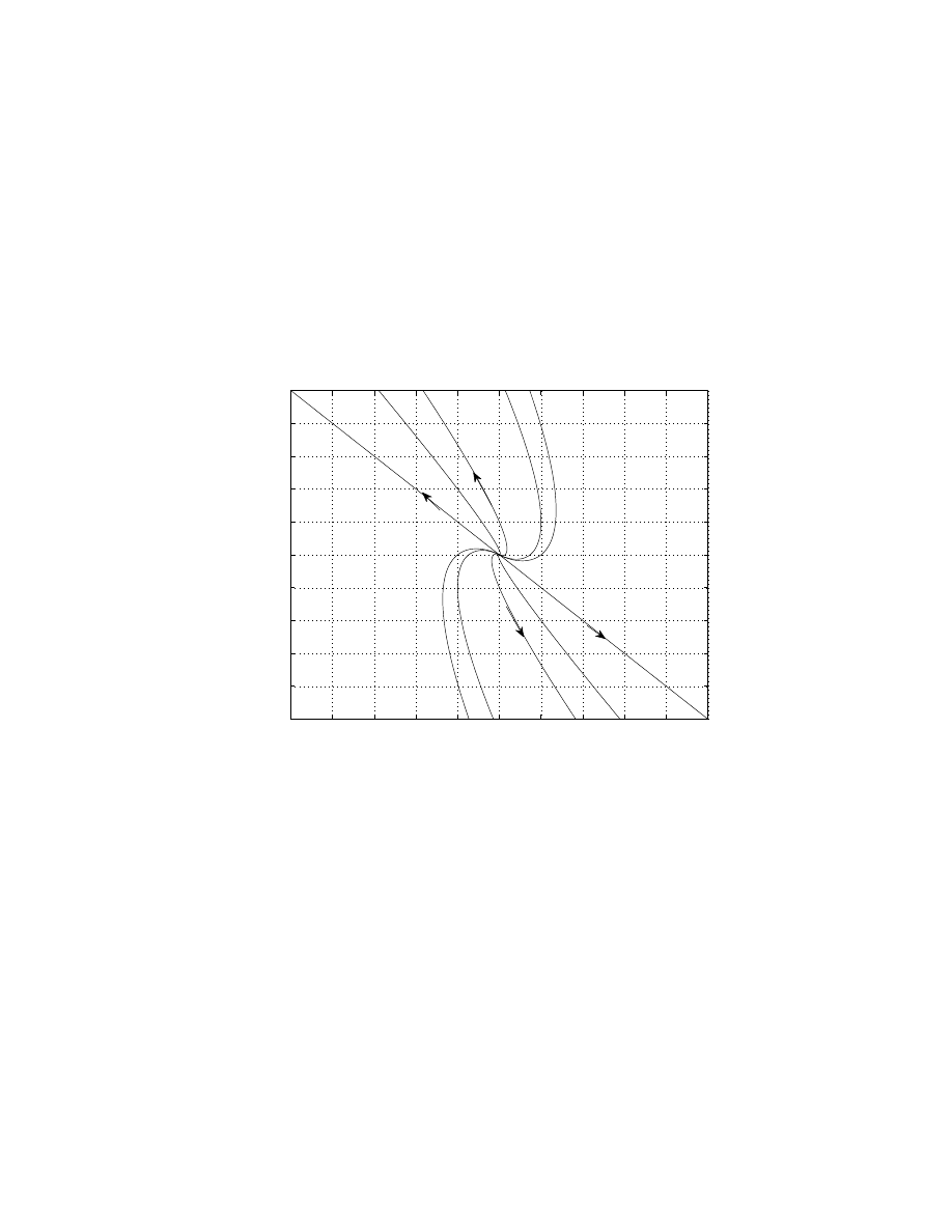
• For the general case, with c
1
6= 0 and c
2
6= 0, a similar thing happens.
As t → ∞, the dominant term in ~x is te
λt
~v. This means the solution
approach the direction of ~v. As t → −∞, the dominant term in ~x is
still te
λt
~v. This means the solution approach the direction of ~v. But,
due to the change of sign of t, the ~x will change direction and point
toward the opposite direction as when t → ∞. See plot below.
−5
−4
−3
−2
−1
0
1
2
3
4
5
−5
−4
−3
−2
−1
0
1
2
3
4
5
x
1
x
2
z
1
z
2
Remark: If λ < 0, the phase portrait looks the same except with reversed
arrows.
Definition
. If A has repeated eigenvalues, the origin is called a improper
node. It is stable if λ < 0, and unstable if λ > 0.
Example
2. Find the general solution to the system ~x
′
=
−2
2
−0.5 −4
~x.
We start with finding the eigenvalues:
det(A−λI) = (−2−λ)(−4−λ)+1 = λ
2
+6λ+8+1 = (λ+3)
2
= 0,
λ
1
= λ
2
= λ = −3
117
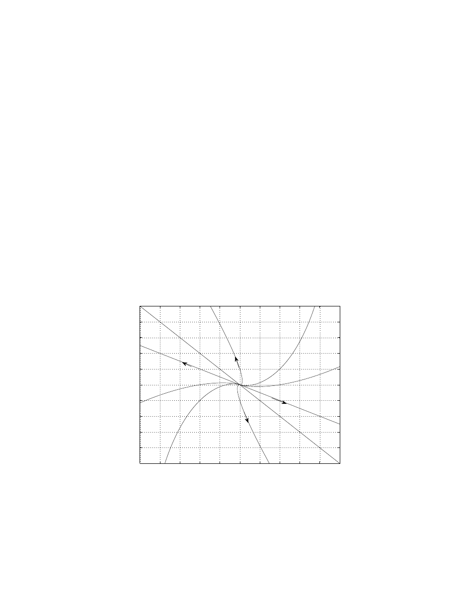
We see we have double eigenvalue. The corresponding eigenvector ~v = (a, b)
T
(A − λI)~v =
−2 + 3
2
−0.5
−4 + 3
·
a
b
=
1
2
−0.5 −1
·
a
b
= 0
So we must have a + 2b = 0. Choose a = 2, then b = −1, and we get
~v =
2
−1
. To find the generalized eigenvector ~η, we solve
(A − λI)~η = ~v,
1
2
−0.5 −1
·
η
1
η
2
=
2
−1
.
This gives us one relation η
1
+ 2η
2
= 2. Choose η
1
= 0, then we have η
2
= 1,
and so ~η =
0
1
. The general solution is
~x = c
1
e
λt
~v + c
2
(te
λt
~v + e
λt
~η) = c
1
e
3t
2
−1
+ c
2
te
3t
2
−1
+ e
3t
0
1
.
Just for fun, I include the phase portrait below.
−5
−4
−3
−2
−1
0
1
2
3
4
5
−5
−4
−3
−2
−1
0
1
2
3
4
5
x
1
x
2
z
1
z
2
The origin is an improper node which is unstable.
118

Summary of the chapter
:
λ
1,2
eigenvalues
type of origin
stability
real
λ
1
· λ
2
< 0
saddle point
unstable
real
λ
1
> 0, λ
2
> 0, λ
1
6= λ
2
node (source)
unstable
real
λ
1
< 0, λ
2
< 0, λ
1
6= λ
2
node (sink)
stable
real
λ
1
= λ
2
= λ
improper node
stable if λ < 0, unstable if λ > 0
complex
λ
1,2
= i ± β
center
stable but not asymptotically
complex
λ
1,2
= α ± iβ
spiral point
stable if α < 0, unstable if α > 0
119
Wyszukiwarka
Podobne podstrony:
G B Folland Lectures on Partial Differential Equations
G B Folland Lectures on Partial Differential Equations
CALC1 L 11 12 Differenial Equations
Evans L C Introduction To Stochastic Differential Equations
Complex Numbers and Ordinary Differential Equations 36 pp
Mathematics HL paper 3 series and differential equations 001
Mathematics HL paper 3 series and differential equations
The algorithm of solving differential equations in continuous model of tall buildings subjected to c
An introduction to difference equation by Elaydi 259
CALC1 L 11 12 Differenial Equations
Evans L C Introduction To Stochastic Differential Equations
Grigoryan V Partial differential equations (draft, UCSB, 2010)(O)(96s) MCde
Olver Lie Groups & Differential Equations (2001) [sharethefiles com]
Bradley Numerical Solutions of Differential Equations [sharethefiles com]
Linearization of nonlinear differential equation by Taylor series expansion
Using Matlab for Solving Differential Equations (jnl article) (1999) WW
Partial Differential Equations (excerpt from larger) (2001) WW
więcej podobnych podstron