F

ORMAL

M

ETHODS

L

ECTURE

IV: C

OMPUTATION

T

REE

L

OGIC

(CTL)

Alessandro Artale

Faculty of Computer Science – Free University of Bolzano

[e-mail]

http://www.inf.unibz.it/

∼artale/

Some material (text, figures) displayed in these slides is courtesy of:

M. Benerecetti, A. Cimatti, M. Fisher, F. Giunchiglia, M. Pistore, M. Roveri, R.Sebastiani.

Alessandro Artale (FM – First Semester – 2009/2010) – p. 1/37

Summary of Lecture IV

Computation Tree Logic: Intuitions.

CTL: Syntax and Semantics.

CTL in Computer Science.

CTL and Model Checking: Examples.

CTL Vs. LTL.

CTL*.

Alessandro Artale (FM – First Semester – 2009/2010) – p. 2/37

Computation Tree logic Vs. LTL

LTL implicitly quantifies universally over paths.

h

K M

, si |= φ iff

for every path

π starting at s

h

K M

, πi |= φ

Properties that assert the existence of a path cannot be
expressed. In particular, properties which mix existential
and universal path quantifiers cannot be expressed.

The Computation Tree Logic, CTL, solves these
problems!

•

CTL explicitly introduces path quantifiers!

•

CTL is the natural temporal logic interpreted over

Branching Time Structures.

Alessandro Artale (FM – First Semester – 2009/2010) – p. 3/37

CTL at a glance

CTL is evaluated over branching-time structures

(Trees).

CTL explicitly introduces path quantifiers:

All Paths

:

P

Exists a Path

:

♦

P

.

Every temporal operator

(

,

♦

,

k

,

U

) preceded by a

path quantifier (

P

or

♦

P

).

Universal modalities:

P

♦

,

P

,

P

k

,

P

U

The temporal formula is true in all the paths starting in
the current state.

Existential modalities:

♦

P

♦

,

♦

P

,

♦

P

k

,

♦

P

U

The temporal formula is true in some path starting in
the current state.

Alessandro Artale (FM – First Semester – 2009/2010) – p. 4/37

Summary

Computation Tree Logic: Intuitions.

CTL: Syntax and Semantics.

CTL in Computer Science.

CTL and Model Checking: Examples.

CTL Vs. LTL.

CTL*.

Alessandro Artale (FM – First Semester – 2009/2010) – p. 5/37

CTL: Syntax

Countable set Σ of atomic propositions: p

, q, . . . the set F

ORM

of formulas is:

ϕ

, ψ →

p

| ⊤ | ⊥ | ¬ϕ | ϕ ∧ ψ | ϕ ∨ ψ |

P

k

ϕ

|

P

ϕ

|

P

♦

ϕ

|

P

(ϕ

U

ψ

)

♦

P

k

ϕ

|

♦

P

ϕ

|

♦

P

♦

ϕ

|

♦

P

(ϕ

U

ψ

)

Alessandro Artale (FM – First Semester – 2009/2010) – p. 6/37

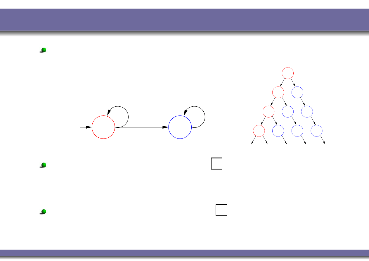
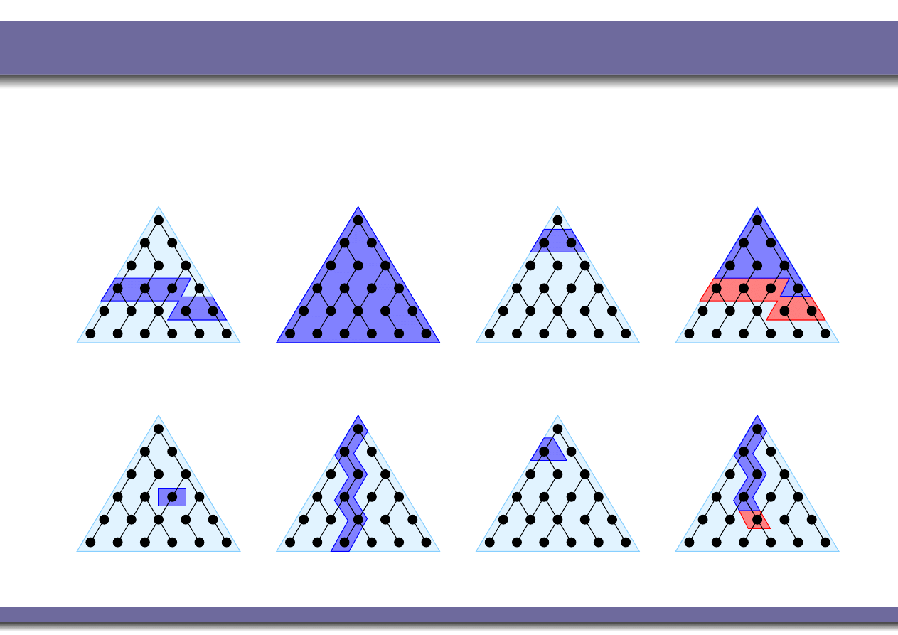
CTL: Semantics

We interpret our CTL temporal formulas over Kripke
Models linearized as trees.

done

!done

done

done

done

done

done

done

!done

!done

!done

!done

Universal modalities

(

P

♦

,

P

,

P

k

,

P

U

): the

temporal formula is true in all the paths starting in the
current state.

Existential modalities

(

♦

P

♦

,

♦

P

,

♦

P

k

,

♦

P

U

): the

temporal formula is true in some path starting in the
current state.

Alessandro Artale (FM – First Semester – 2009/2010) – p. 7/37

CTL: Semantics (Cont.)

Let Σ be a set of atomic propositions. We interpret our CTL
temporal formulas over Kripke Models:

K M

= hS, I, R, Σ, Li

The semantics of a temporal formula is provided by the
satisfaction

relation:

|= : (

K M

× S × F

ORM

) → {true, false}

Alessandro Artale (FM – First Semester – 2009/2010) – p. 8/37

CTL Semantics: The Propositional Aspect

We start by defining when an atomic proposition is true at a
state/time “s

i

”

K M

, s

i

|= p

iff

p

∈ L(s

i

)

(for p

∈ Σ)

The semantics for the classical operators is as expected:

K M

, s

i

|= ¬ϕ

iff

K M

, s

i

6|= ϕ

K M

, s

i

|= ϕ ∧ ψ

iff

K M

, s

i

|= ϕ and

K M

, s

i

|= ψ

K M

, s

i

|= ϕ ∨ ψ

iff

K M

, s

i

|= ϕ or

K M

, s

i

|= ψ

K M

, s

i

|= ϕ ⇒ ψ iff

if

K M

, s

i

|= ϕ then

K M

, s

i

|= ψ

K M

, s

i

|= ⊤

K M

, s

i

6|= ⊥

Alessandro Artale (FM – First Semester – 2009/2010) – p. 9/37

CTL Semantics: The Temporal Aspect

Temporal operators have the following semantics where
π

= (s

i

, s

i

+1

, . . .) is a generic path outgoing from state s

i

in

K M

.

K M

, s

i

|=

P

j

ϕ

iff

∀π = (s

i

, s

i

+1

, . . .)

K M

, s

i

+1

|= ϕ

K M

, s

i

|=

♦

P

j

ϕ

iff

∃π = (s

i

, s

i

+1

, . . .)

K M

, s

i

+1

|= ϕ

K M

, s

i

|=

P

ϕ

iff

∀π = (s

i

, s

i

+1

, . . .) ∀ j ≥ i.

K M

, s

j

|= ϕ

K M

, s

i

|=

♦

P

ϕ

iff

∃π = (s

i

, s

i

+1

, . . .) ∀ j ≥ i.

K M

, s

j

|= ϕ

K M

, s

i

|=

P

♦

ϕ

iff

∀π = (s

i

, s

i

+1

, . . .) ∃ j ≥ i.

K M

, s

j

|= ϕ

K M

, s

i

|=

♦

P

♦

ϕ

iff

∃π = (s

i

, s

i

+1

, . . .) ∃ j ≥ i.

K M

, s

j

|= ϕ

K M

, s

i

|=

P

(ϕ

U

ψ

) iff ∀π = (s

i

, s

i

+1

, . . .) ∃ j ≥ i.

K M

, s

j

|= ψ and

∀i ≤ k < j : M, s

k

|= ϕ

K M

, s

i

|=

♦

P

(ϕ

U

ψ

) iff ∃π = (s

i

, s

i

+1

, . . .) ∃ j ≥ i.

K M

, s

j

|= ψ and

∀i ≤ k < j :

K M

, s

k

|= ϕ

Alessandro Artale (FM – First Semester – 2009/2010) – p. 10/37

CTL Semantics: Intuitions

CTL is given by the standard boolean logic enhanced with

temporal operators.

⊲ “

Necessarily Next

”.

P

k

ϕ is true in s

t

iff ϕ is true in every

successor state s

t

+1

⊲ “

Possibly Next

”.

♦

P

k

ϕ is true in s

t

iff ϕ is true in one

successor state s

t

+1

⊲ “

Necessarily in the future

” (or “Inevitably”).

P

♦

ϕ is true in s

t

iff ϕ is inevitably true in some s

t

′

with t

′

≥ t

⊲ “

Possibly in the future

” (or “Possibly”).

♦

P

♦

ϕ is true in s

t

iff ϕ

may be true in some s

t

′

with t

′

≥ t

Alessandro Artale (FM – First Semester – 2009/2010) – p. 11/37

CTL Semantics: Intuitions (Cont.)

⊲ “

Globally

” (or “always”).

P

ϕ is true in s

t

iff ϕ is true in all

s

t

′

with t

′

≥ t

⊲ “

Possibly henceforth

”.

♦

P

ϕ is true in s

t

iff ϕ is possibly true

henceforth

⊲ “

Necessarily Until

”.

P

(ϕ

U

ψ

) is true in s

t

iff necessarily ϕ

holds until ψ holds.

⊲ “

Possibly Until

”.

♦

P

(ϕ

U

ψ

) is true in s

t

iff possibly ϕ holds

until ψ holds.

Alessandro Artale (FM – First Semester – 2009/2010) – p. 12/37

CTL Alternative Notation

Alternative notations are used for temporal operators.

♦

P

E

there

E

xists a path

P

A

in

A

ll paths

♦

F

sometime in the

F

uture

G

G

lobally in the future

k

X

ne

X

time

Alessandro Artale (FM – First Semester – 2009/2010) – p. 13/37

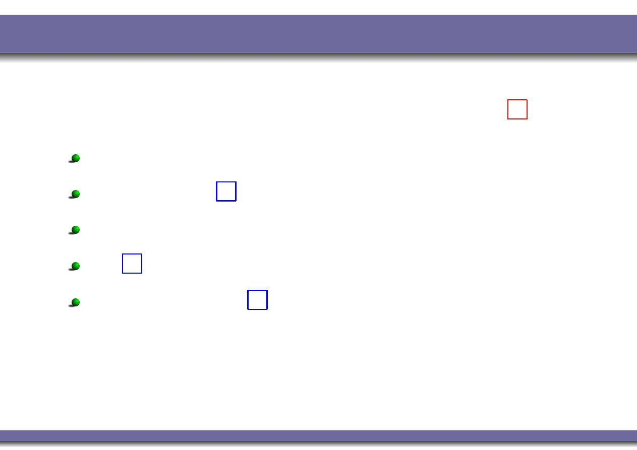
CTL Semantics: Intuitions (Cont.)

P

finally

P

globally

P

next

P

until

q

P

EF

P

EX

P

U

q

]

E[

P

EG

AF

P

AX

P

P

U

q

A[

]

AG

P

Alessandro Artale (FM – First Semester – 2009/2010) – p. 14/37

A Complete Set of CTL Operators

All CTL operators can be expressed via:

♦

P

k

,

♦

P

,

♦

P

U

P

k

ϕ

≡ ¬

♦

P

k

¬ϕ

P

♦

ϕ

≡ ¬

♦

P

¬ϕ

♦

P

♦

ϕ

≡

♦

P

(⊤

U

ϕ

)

P

ϕ

≡ ¬

♦

P

♦

¬ϕ ≡ ¬

♦

P

(⊤

U

¬ϕ)

P

(ϕ

U

ψ

) ≡ ¬

♦

P

¬ψ ∧ ¬

♦

P

(¬ψ

U

(¬ϕ ∧ ¬ψ))

Alessandro Artale (FM – First Semester – 2009/2010) – p. 15/37

Summary

Computation Tree Logic: Intuitions.

CTL: Syntax and Semantics.

CTL in Computer Science.

CTL and Model Checking: Examples.

CTL Vs. LTL.

CTL*.

Alessandro Artale (FM – First Semester – 2009/2010) – p. 16/37

Safety Properties

Safety:

“something bad will not happen”

Typical examples:

P

¬(reactor_temp > 1000)

P

¬(one_way ∧

P

k

other

_way

)

P

¬((x = 0) ∧

P

k

P

k

P

k

(y = z/x))

and so on.....

Usually:

P

¬....

Alessandro Artale (FM – First Semester – 2009/2010) – p. 17/37

Liveness Properties

Liveness:

“something good will happen”

Typical examples:

P

♦

rich

P

♦

(x > 5)

P

(start ⇒

P

♦

terminate

)

and so on.....

Usually:

P

♦

. . .

Alessandro Artale (FM – First Semester – 2009/2010) – p. 18/37

Fairness Properties

Often only really useful when scheduling processes,
responding to messages, etc.

Fairness:

“something is successful/allocated infinitely often”

Typical example:

P

(

P

♦

enabled

)

Usually:

P

P

♦

. . .

Alessandro Artale (FM – First Semester – 2009/2010) – p. 19/37

Summary

Computation Tree Logic: Intuitions.

CTL: Syntax and Semantics.

CTL in Computer Science.

CTL and Model Checking: Examples.

CTL Vs. LTL.

CTL*.

Alessandro Artale (FM – First Semester – 2009/2010) – p. 20/37

The CTL Model Checking Problem

The CTL Model Checking Problem is formulated as:

K M

|= φ

Check if

K M

, s

0

|= φ, for every initial state, s

0

, of the Kripke

structure

K M

.

Alessandro Artale (FM – First Semester – 2009/2010) – p. 21/37

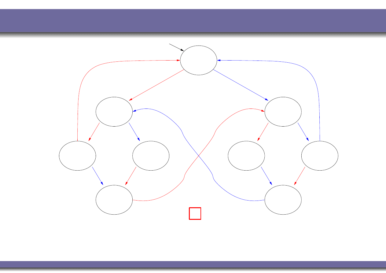
Example 1: Mutual Exclusion (Safety)

N1, N2

turn=0

turn=1

C1, T2

turn=1

T1, T2

T1, N2

turn=1

C1, N2

turn=1

T1, T2

turn=2

N = noncritical, T = trying, C = critical

User 1

User 2

N1, T2

turn=2

T1, C2

turn=2

turn=2

N1, C2

K M

|=

P

¬(C

1

∧C

2

)

?

Alessandro Artale (FM – First Semester – 2009/2010) – p. 22/37

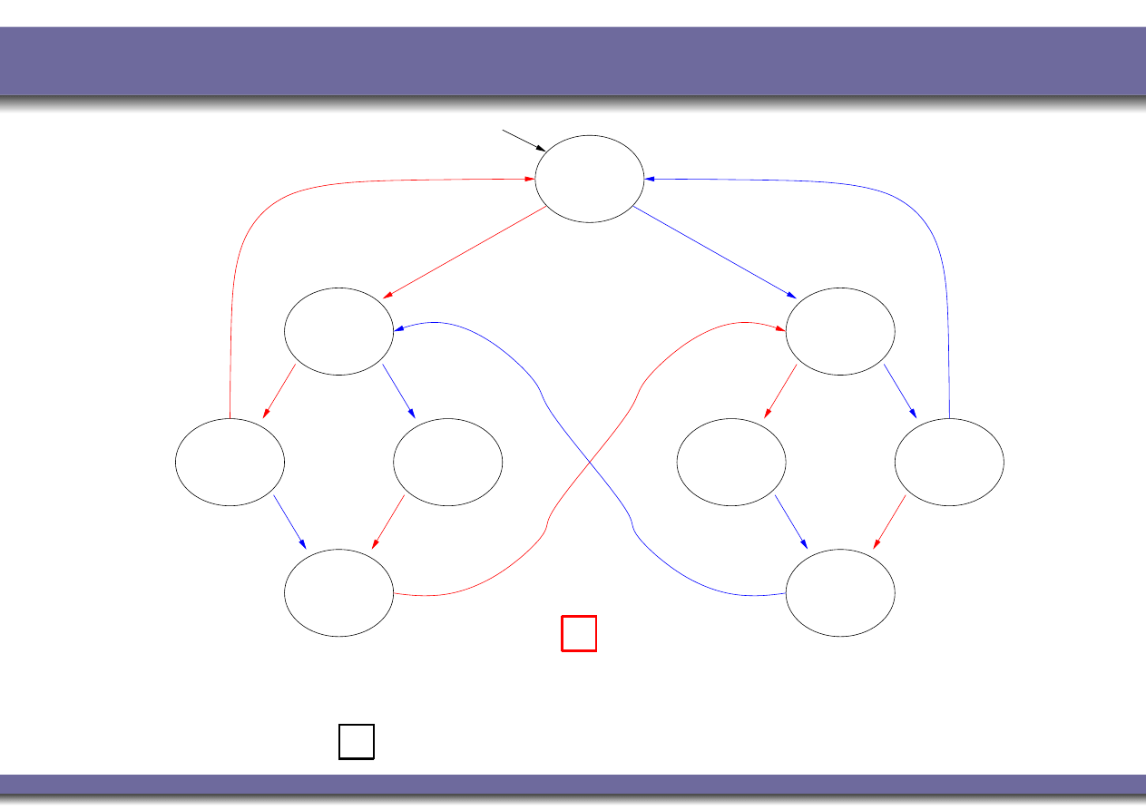
Example 1: Mutual Exclusion (Safety)

N1, N2

turn=0

turn=1

C1, T2

turn=1

T1, T2

T1, N2

turn=1

C1, N2

turn=1

T1, T2

turn=2

N = noncritical, T = trying, C = critical

User 1

User 2

N1, T2

turn=2

T1, C2

turn=2

turn=2

N1, C2

K M

|=

P

¬(C

1

∧C

2

)

?

YES

: There is no reachable state in which

(C

1

∧C

2

) holds!

(Same as the

¬(C

1

∧C

2

) in LTL.)

Alessandro Artale (FM – First Semester – 2009/2010) – p. 22/37

Example 2: Liveness

N1, N2

turn=0

turn=1

C1, T2

turn=1

T1, T2

T1, N2

turn=1

C1, N2

turn=1

T1, T2

turn=2

N = noncritical, T = trying, C = critical

User 1

User 2

N1, T2

turn=2

T1, C2

turn=2

turn=2

N1, C2

K M

|=

P

(T

1

⇒

P

♦

C

1

)

?

Alessandro Artale (FM – First Semester – 2009/2010) – p. 23/37

Example 2: Liveness

N1, N2

turn=0

turn=1

C1, T2

turn=1

T1, T2

T1, N2

turn=1

C1, N2

turn=1

T1, T2

turn=2

N = noncritical, T = trying, C = critical

User 1

User 2

N1, T2

turn=2

T1, C2

turn=2

turn=2

N1, C2

K M

|=

P

(T

1

⇒

P

♦

C

1

)

?

YES

: every path starting from each state where T

1

holds

passes through a state where C

1

holds.

(Same as

(T

1

⇒

♦

C

1

) in LTL)

Alessandro Artale (FM – First Semester – 2009/2010) – p. 23/37

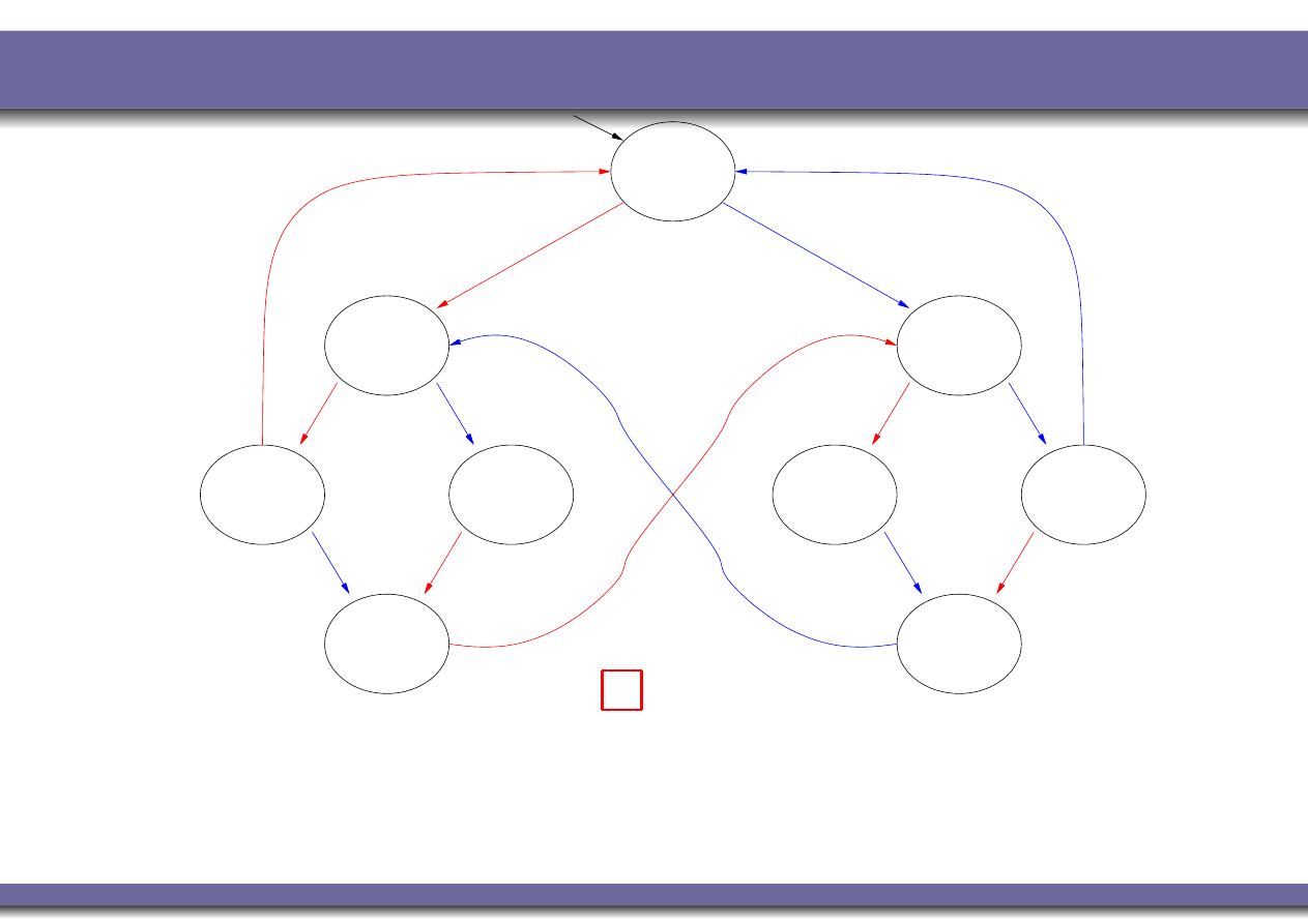
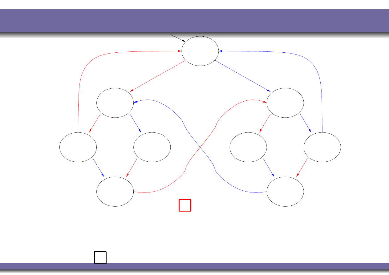
Example 3: Fairness

N1, N2

turn=0

turn=1

C1, T2

turn=1

T1, T2

T1, N2

turn=1

C1, N2

turn=1

T1, T2

turn=2

N = noncritical, T = trying, C = critical

User 1

User 2

N1, T2

turn=2

T1, C2

turn=2

turn=2

N1, C2

K M

|=

P

P

♦

C

1

?

Alessandro Artale (FM – First Semester – 2009/2010) – p. 24/37

Example 3: Fairness

N1, N2

turn=0

turn=1

C1, T2

turn=1

T1, T2

T1, N2

turn=1

C1, N2

turn=1

T1, T2

turn=2

N = noncritical, T = trying, C = critical

User 1

User 2

N1, T2

turn=2

T1, C2

turn=2

turn=2

N1, C2

K M

|=

P

P

♦

C

1

?

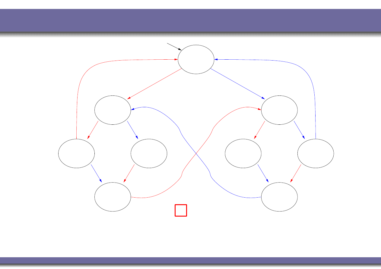
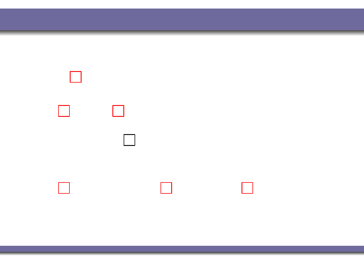
NO

: e.g., in the initial state, there is the blue cyclic path in

which C

1

never holds! (Same as

♦

C

1

in LTL)

Alessandro Artale (FM – First Semester – 2009/2010) – p. 24/37

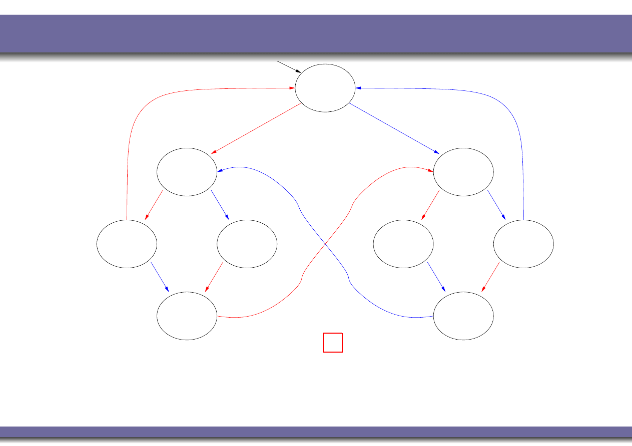
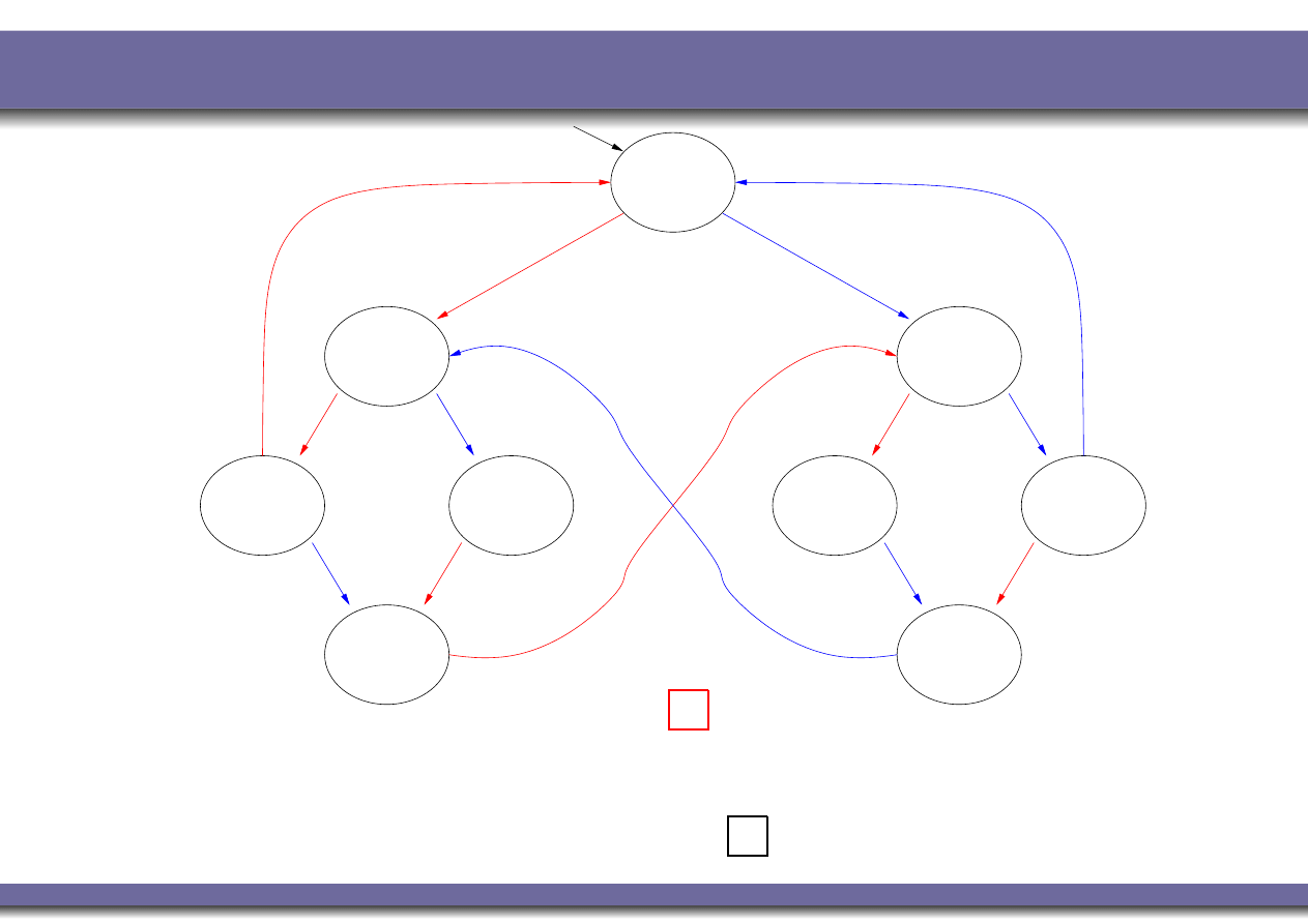
Example 4: Non-Blocking

N1, N2

turn=0

turn=1

C1, T2

turn=1

T1, T2

T1, N2

turn=1

C1, N2

turn=1

T1, T2

turn=2

N = noncritical, T = trying, C = critical

User 1

User 2

N1, T2

turn=2

T1, C2

turn=2

turn=2

N1, C2

K M

|=

P

(N

1

⇒

♦

P

♦

T

1

)

?

Alessandro Artale (FM – First Semester – 2009/2010) – p. 25/37

Example 4: Non-Blocking

N1, N2

turn=0

turn=1

C1, T2

turn=1

T1, T2

T1, N2

turn=1

C1, N2

turn=1

T1, T2

turn=2

N = noncritical, T = trying, C = critical

User 1

User 2

N1, T2

turn=2

T1, C2

turn=2

turn=2

N1, C2

K M

|=

P

(N

1

⇒

♦

P

♦

T

1

)

?

YES

: from each state where N

1

holds there is a path leading

to a state where T

1

holds. (No corresponding LTL formulas)

Alessandro Artale (FM – First Semester – 2009/2010) – p. 25/37

Summary

Computation Tree Logic: Intuitions.

CTL: Syntax and Semantics.

CTL in Computer Science.

CTL and Model Checking: Examples.

CTL Vs. LTL.

CTL*.

Alessandro Artale (FM – First Semester – 2009/2010) – p. 26/37

LTL Vs. CTL: Expressiveness

⊲ Many CTL formulas cannot be expressed in LTL

(e.g., those containing paths quantified existentially)
E.g.,

P

(N

1

⇒

♦

P

♦

T

1

)

⊲ Many LTL formulas cannot be expressed in CTL

E.g.,

♦

T

1

⇒

♦

C

1

(Strong Fairness in LTL)

i.e, formulas that select a range of paths with a property
(

♦

p

⇒

♦

q

Vs.

P

(p ⇒

P

♦

q

))

⊲ Some formluas can be expressed both in LTL and in CTL

(typically LTL formulas with operators of nesting depth 1)
E.g.,

¬(C

1

∧C

2

),

♦

C

1

,

(T

1

⇒

♦

C

1

),

♦

C

1

Alessandro Artale (FM – First Semester – 2009/2010) – p. 27/37

LTL Vs. CTL: Expressiveness (Cont.)

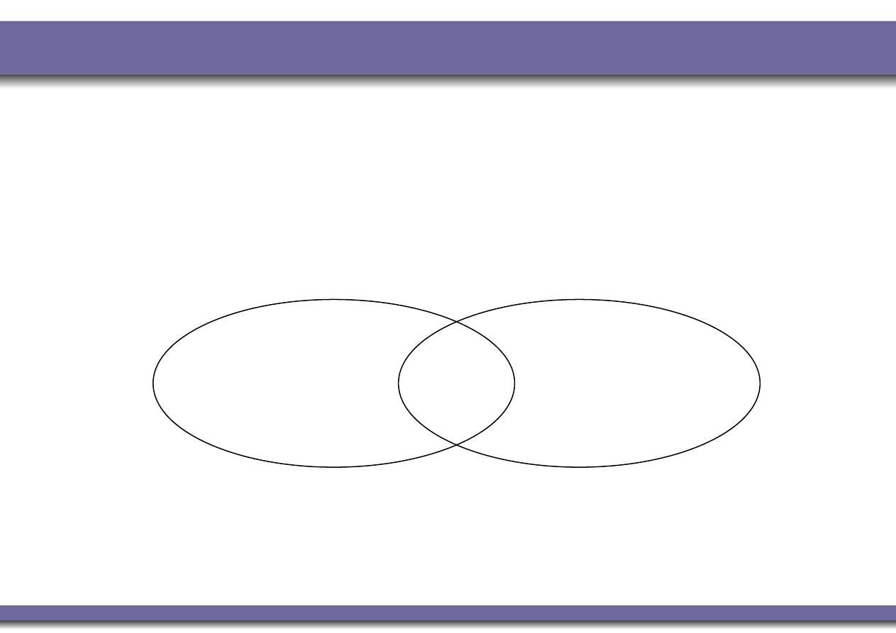
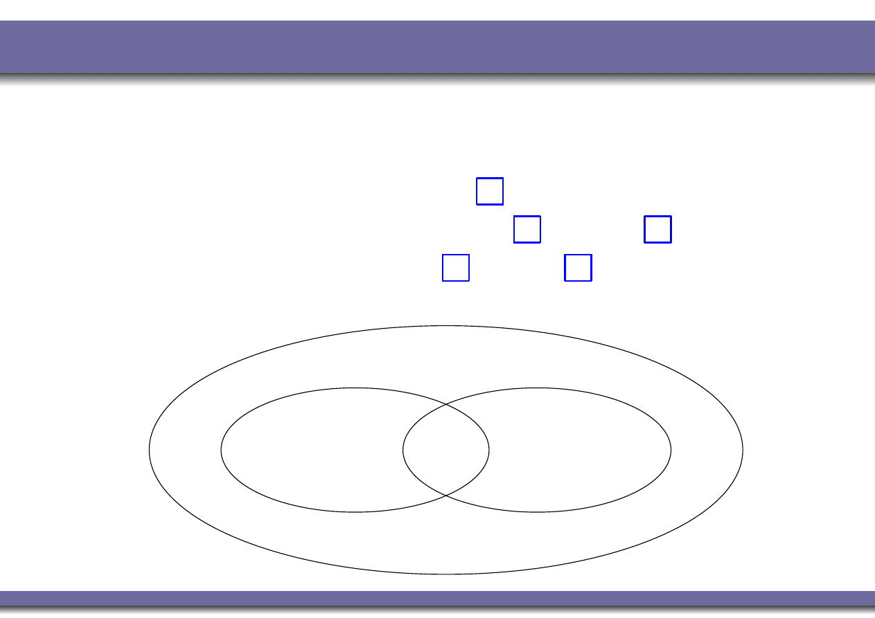
CTL and LTL have incomparable expressive power.

The choice between LTL and CTL depends on the
application and the personal preferences.

CTL

LTL

Alessandro Artale (FM – First Semester – 2009/2010) – p. 28/37

Summary

Computation Tree Logic: Intuitions.

CTL: Syntax and Semantics.

CTL in Computer Science.

CTL and Model Checking: Examples.

CTL Vs. LTL.

CTL*.

Alessandro Artale (FM – First Semester – 2009/2010) – p. 29/37

The Computation Tree Logic CTL*

CTL* is a logic that combines the expressive power of
LTL and CTL.

Temporal operators can be applied without any
constraints.

•

P

(

k

ϕ

∨

k k

ϕ

)

.

Along all paths, ϕ is true in the next state or the next two
steps.

•

♦

P

(

♦

ϕ

)

.

There is a path along which ϕ is infinitely often true.

Alessandro Artale (FM – First Semester – 2009/2010) – p. 30/37

CTL*: Syntax

Countable set Σ of atomic propositions: p

, q, . . . we

distinguish between

States Formulas

(evaluated on states):

ϕ

, ψ →

p

| ⊤ | ⊥ | ¬ϕ | ϕ ∧ ψ | ϕ ∨ ψ |

P

α

|

♦

P

α

and

Path Formulas

(evaluated on paths):

α

, β →

ϕ

|

¬α | α ∧ β | α ∨ β |

k

α

|

α

|

♦

α

|

(α

U

β

)

The set of CTL* formulas F

ORM

is the set of state formulas.

Alessandro Artale (FM – First Semester – 2009/2010) – p. 31/37

CTL* Semantics: State Formulas

We start by defining when an atomic proposition is true at a
state “s

0

”

K M

, s

0

|= p iff

p

∈ L(s

0

)

(for p

∈ Σ)

The semantics for State Formulas is the following where
π

= (s

0

, s

1

, . . .) is a generic path outgoing from state s

0

:

K M

, s

0

|= ¬ϕ

iff

K M

, s

0

6|= ϕ

K M

, s

0

|= ϕ ∧ ψ

iff

K M

, s

0

|= ϕ and

K M

, s

0

|= ψ

K M

, s

0

|= ϕ ∨ ψ

iff

K M

, s

0

|= ϕ or

K M

, s

0

|= ψ

K M

, s

0

|=

♦

P

α

iff

∃π = (s

0

, s

1

, . . .) such that

K M

, π |= α

K M

, s

0

|=

P

α

iff

∀π = (s

0

, s

1

, . . .) then

K M

, π |= α

Alessandro Artale (FM – First Semester – 2009/2010) – p. 32/37

CTL* Semantics: Path Formulas

The semantics for Path Formulas is the following where
π

= (s

0

, s

1

, . . .) is a generic path outgoing from state s

0

and π

i

denotes the suffix path

(s

i

, s

i

+1

, . . .):

K M

, π |= ϕ

iff

K M

, s

0

|= ϕ

K M

, π |= ¬α

iff

K M

, π 6|= α

K M

, π |= α ∧ β

iff

K M

, π |= α and

K M

, π |= β

K M

, π |= α ∨ β

iff

K M

, π |= α or

K M

, π |= β

K M

, π |=

♦

α

iff

∃i ≥ 0 such that

K M

, π

i

|= α

K M

, π |=

α

iff

∀i ≥ 0 then

K M

, π

i

|= α

K M

, π |=

k

α

iff

K M

, π

1

|= α

K M

, π |= α

U

β

iff

∃i ≥ 0 such that

K M

, π

i

|= β and

∀ j.(0 ≤ j ≤ i) then

K M

, π

j

|= α

Alessandro Artale (FM – First Semester – 2009/2010) – p. 33/37

CTLs Vs LTL Vs CTL: Expressiveness

CTL* subsumes both CTL and LTL

⊲ ϕ in CTL =⇒ ϕ in CTL* (e.g.,

P

(N

1

⇒

♦

P

♦

T

1

)

)

⊲ ϕ in LTL =⇒

P

ϕ in CTL* (e.g.,

P

(

♦

T

1

⇒

♦

C

1

)

)

⊲ LTL ∪ CTL ⊂ CTL* (e.g.,

♦

P

(

♦

p

⇒

♦

q

)

)

CTL

LTL

CTL*

Alessandro Artale (FM – First Semester – 2009/2010) – p. 34/37

CTL* Vs LTL Vs CTL: Complexity

The following Table shows the Computational Complexity of
checking Satisbiability

Logic

Complexity

LTL

PSpace-Complete

CTL

ExpTime-Complete

CTL*

2ExpTime-Complete

Alessandro Artale (FM – First Semester – 2009/2010) – p. 35/37

CTL* Vs LTL Vs CTL: Complexity (Cont.)

The following Table shows the Computational Complexity of
Model Checking (M.C.)

•

Since M.C. has 2 inputs – the model,

M

, and the

formula, ϕ – we give two complexity measures.

Logic

Complexity w.r.t.

| ϕ |

Complexity w.r.t.

|

M

|

LTL

PSpace-Complete

P (linear)

CTL

P-Complete

P (linear)

CTL*

PSpace-Complete

P (linear)

Alessandro Artale (FM – First Semester – 2009/2010) – p. 36/37

Summary of Lecture IV

Computation Tree Logic: Intuitions.

CTL: Syntax and Semantics.

CTL in Computer Science.

CTL and Model Checking: Examples.

CTL Vs. LTL.

CTL*.

Alessandro Artale (FM – First Semester – 2009/2010) – p. 37/37