F

ORMAL

M

ETHODS

L

ECTURE

III: L

INEAR

T

EMPORAL

L

OGIC

Alessandro Artale

Faculty of Computer Science – Free University of Bolzano

[e-mail]

http://www.inf.unibz.it/

∼artale/

Some material (text, figures) displayed in these slides is courtesy of:

M. Benerecetti, A. Cimatti, M. Fisher, F. Giunchiglia, M. Pistore, M. Roveri, R.Sebastiani.

Alessandro Artale (FM – First Semester – 2009/2010) – p. 1/39

Summary of Lecture III

Introducing Temporal Logics.

Intuitions beyond Linear Temporal Logic.

LTL: Syntax and Semantics.

LTL in Computer Science.

LTL Interpreted over Kripke Models.

LTL and Model Checking: Intuitions.

Alessandro Artale (FM – First Semester – 2009/2010) – p. 2/39

An Introduction to Temporal Logics

In classical logic, formulae are evaluated within a single
fixed world.

For example, a proposition such as “it is Monday” must be
either true or false.

Propositions are then combined using constructs such as
‘

∧’, ‘¬’, etc.

But, most (not just computational) systems are

dynamic

.

In temporal logics, evaluation takes place within a

set of

worlds

. Thus, “it is Monday” may be satisfied in some

worlds, but not in others.

Alessandro Artale (FM – First Semester – 2009/2010) – p. 3/39

An Introduction to Temporal Logics (Cont.)

The set of worlds correspond to

moments in time

.

How we navigate between these worlds depends on our
particular view of time.

The particular model of time is captured by a temporal

accessibility relation

between worlds.

Essentially, temporal logic extends classical propositional
logic with a set of

temporal operators

that navigate between

worlds using this accessibility relation.

Alessandro Artale (FM – First Semester – 2009/2010) – p. 4/39

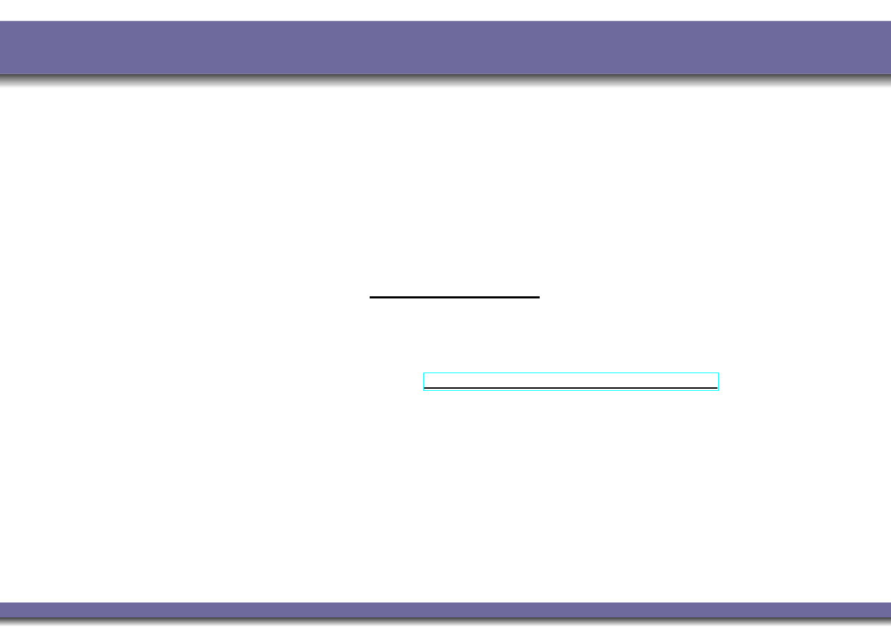
Typical Models of Time

Alessandro Artale (FM – First Semester – 2009/2010) – p. 5/39

Summary

Introducing Temporal Logics.

Intuitions beyond Linear Temporal Logic.

LTL: Syntax and Semantics.

LTL in Computer Science.

LTL Interpreted over Kripke Models.

LTL and Model Checking: Intuitions.

Alessandro Artale (FM – First Semester – 2009/2010) – p. 6/39

Linear Temporal Logic (LTL): Intuitions

Consider a simple temporal logic (LTL) where the
accessibility relation characterises a discrete, linear model
isomorphic to the Natural Numbers.

Typical temporal operators used are

k

ϕ

ϕ is true in the next moment in time

ϕ

ϕ is true in all future moments

♦

ϕ

ϕ is true in some future moment

ϕ

U

ψ

ϕ is true until ψ is true

Examples:

((¬passport ∨ ¬ticket) ⇒

k

¬board_ f light)

Alessandro Artale (FM – First Semester – 2009/2010) – p. 7/39

Computational Example

(requested ⇒

♦

received

)

(received ⇒

k

processed

)

(processed ⇒

♦

done

)

From the above we should be able to infer that it is not the
case that the system continually re-sends a request, but
never sees it completed (

¬done); i.e. the statement

requested

∧

¬done

should be inconsistent.

Alessandro Artale (FM – First Semester – 2009/2010) – p. 8/39

Summary

Introducing Temporal Logics.

Intuitions beyond Linear Temporal Logic.

LTL: Syntax and Semantics.

LTL in Computer Science.

LTL Interpreted over Kripke Models.

LTL and Model Checking: Intuitions.

Alessandro Artale (FM – First Semester – 2009/2010) – p. 9/39

LTL: Syntax

Countable set Σ of atomic propositions: p

, q, . . . the set F

ORM

of formulas is:

ϕ

, ψ →

p

|

(atomic proposition)

⊤ |

(true)

⊥ |

(false)

¬ϕ |

(complement)

ϕ

∧ ψ |

(conjunction)

ϕ

∨ ψ |

(disjunction)

k

ϕ

|

(next time)

ϕ

|

(always)

♦

ϕ

|

(sometime)

ϕ

U

ψ

(until)

Alessandro Artale (FM – First Semester – 2009/2010) – p. 10/39

Temporal Semantics

We interpret our temporal formulae in a discrete, linear
model of time. Formally, this structure is represented by

M

= h

N

,

I

i

where

•

I

:

N

7→ 2

Σ

maps each Natural number (representing a moment in
time) to a set of propositions.

The semantics of a temporal formula is provided by the
satisfaction

relation:

|= : (

M

×

N

× F

ORM

) → {true, false}

Alessandro Artale (FM – First Semester – 2009/2010) – p. 11/39

Semantics: The Propositional Aspect

We start by defining when an atomic proposition is true at a
time point “i”

h

M

, ii |= p iff

p

∈

I

(i)

(for p

∈ Σ)

The semantics for the classical operators is as expected:

h

M

, ii |= ¬ϕ

iff

h

M

, ii 6|= ϕ

h

M

, ii |= ϕ ∧ ψ

iff

h

M

, ii |= ϕ and h

M

, ii |= ψ

h

M

, ii |= ϕ ∨ ψ

iff

h

M

, ii |= ϕ or h

M

, ii |= ψ

h

M

, ii |= ϕ ⇒ ψ iff

if

h

M

, ii |= ϕ then h

M

, ii |= ψ

M

, i |= ⊤

M

, i 6|= ⊥

Alessandro Artale (FM – First Semester – 2009/2010) – p. 12/39

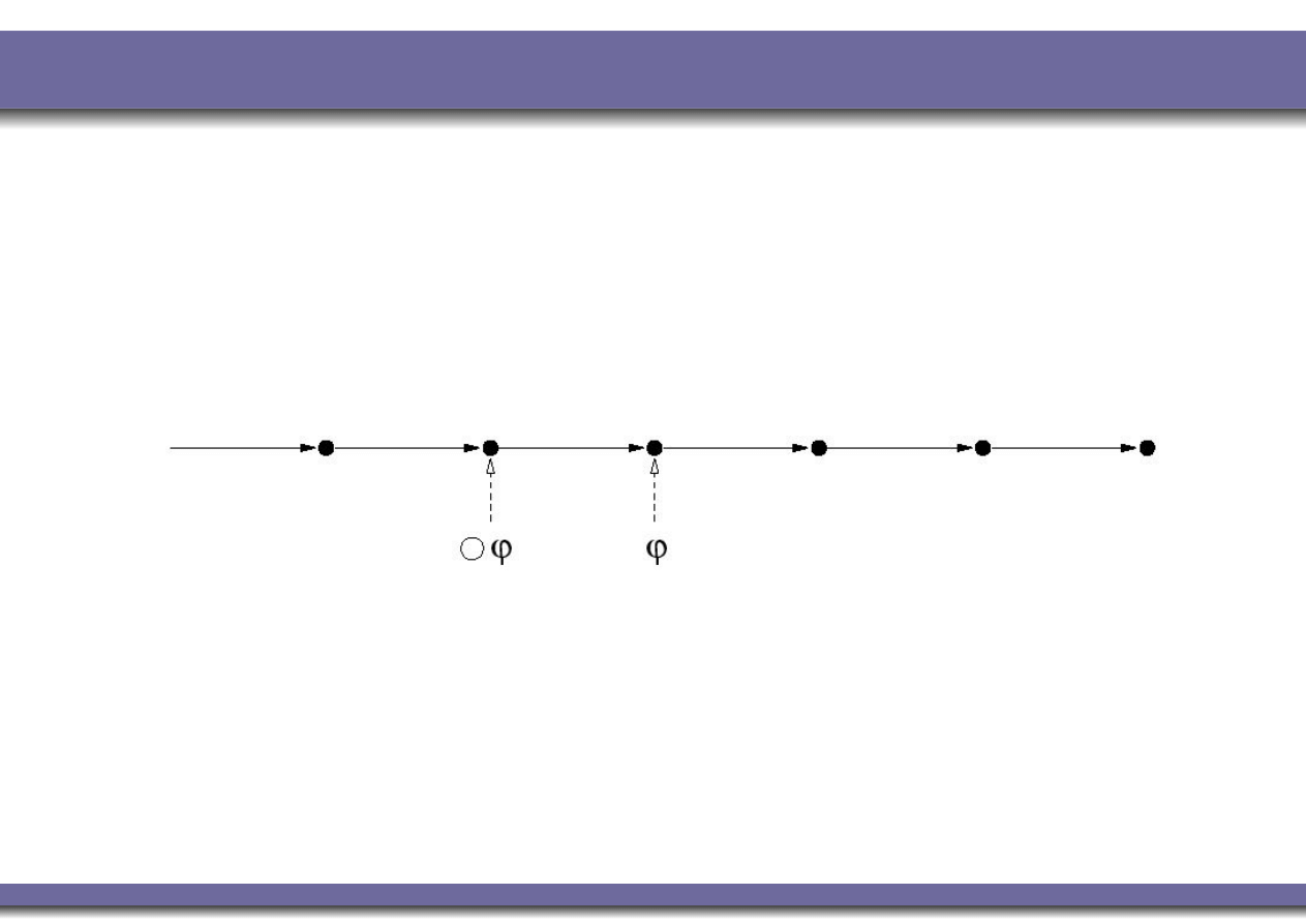
Temporal Operators: ‘next’

h

M

, ii |=

k

ϕ

iff

h

M

, i + 1i |= ϕ

This operator provides a constraint on the next moment in
time.

Examples:

(sad ∧ ¬rich) ⇒

k

sad

((x = 0) ∧ add3) ⇒

k

(x = 3)

Alessandro Artale (FM – First Semester – 2009/2010) – p. 13/39

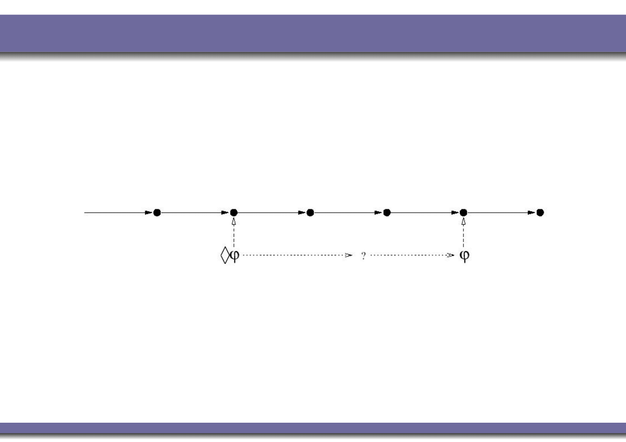
Temporal Operators: ‘sometime’

h

M

, ii |=

♦

ϕ

iff

there exists j

. ( j ≥ i) ∧ h

M

, ji |= ϕ

N.B.

while we can be sure that ϕ will be true either now or in

the future, we can not be sure exactly when it will be true.

Examples:

(¬resigned ∧ sad) ⇒

♦

famous

sad

⇒

♦

happy

send

⇒

♦

receive

Alessandro Artale (FM – First Semester – 2009/2010) – p. 14/39

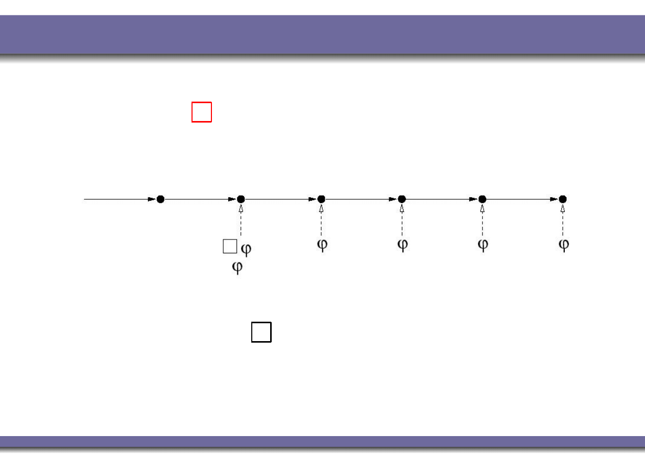
Temporal Operators: ‘always’

h

M

, ii |=

ϕ

iff

for all j

. if ( j ≥ i) then h

M

, ji |= ϕ

This can represent invariant properties.

Examples:

lottery-win

⇒

rich

Alessandro Artale (FM – First Semester – 2009/2010) – p. 15/39

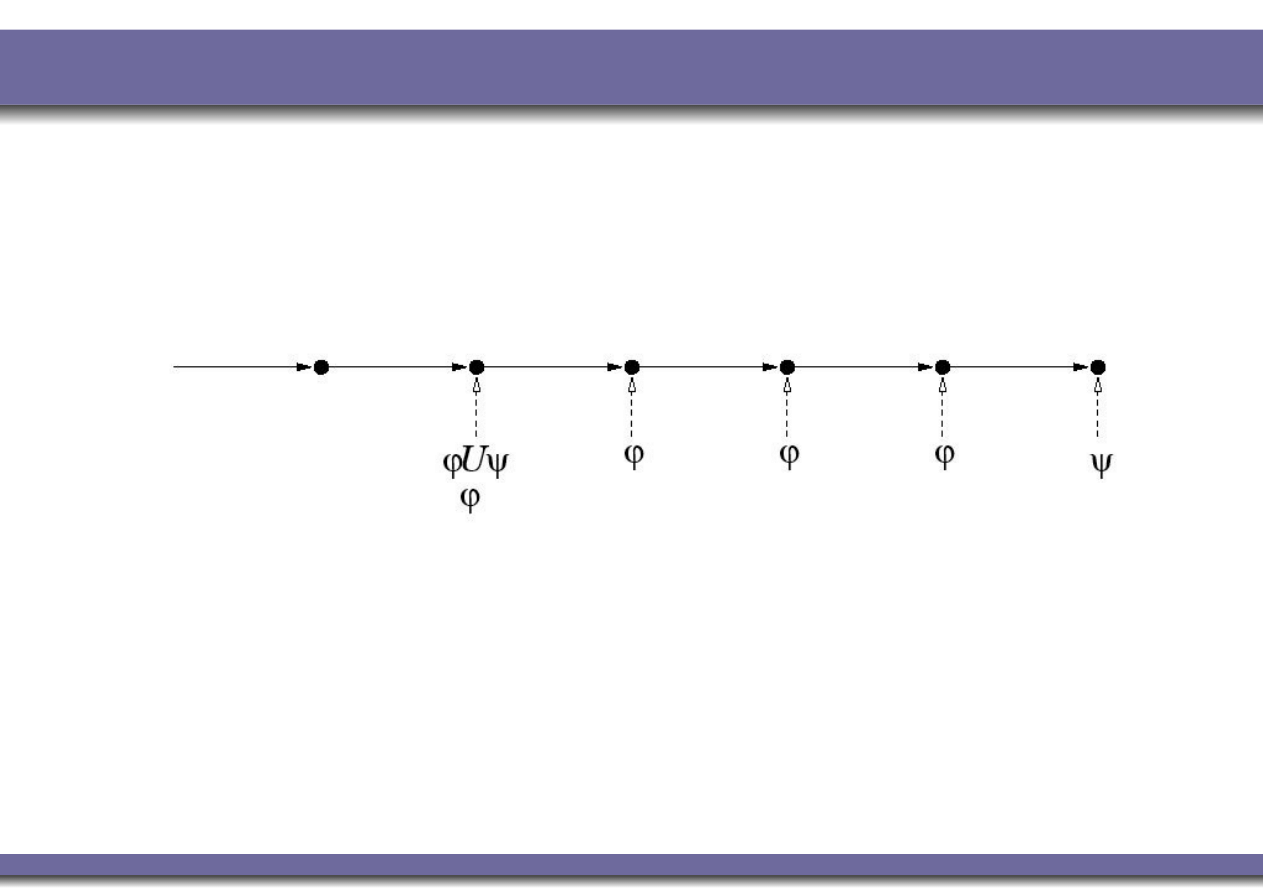
Temporal Operators: ‘until’

h

M

, ii |= ϕ

U

ψ

iff

there exists j

. ( j ≥ i) ∧ h

M

, ji |= ψ ∧

for all k

. (i ≤ k < j) ⇒ h

M

, ki |= ϕ

Examples:

start

_lecture

⇒ talk

U

end

_lecture

born

⇒ alive

U

dead

request

⇒ reply

U

acknowledgement

Alessandro Artale (FM – First Semester – 2009/2010) – p. 16/39

Satisfiability and Validity

A structure

M

= h

N

,

I

i is a model of φ, if

h

M

, ii |= φ, for some i ∈

N

.

Similarly as in classical logic, an LTL formula φ can be
satisfiable

, unsatisfiable or valid. A formula φ is:

Satisfiable

, if there is model for φ.

Unsatisfiable

, if φ is not satisfiable.

Valid

(i.e., a Tautology):

|= φ iff ∀

M

, ∀i ∈

N

. h

M

, ii |= φ.

Alessandro Artale (FM – First Semester – 2009/2010) – p. 17/39

Entailment and Equivalence

Similarly as in classical logic we can define the notions of
entailment

and equivalence between two LTL formulas

Entailment.

φ

|= ψ iff ∀

M

, ∀i ∈

N

.h

M

, ii |= φ ⇒ h

M

, ii |= ψ

Equivalence.

φ

≡ ψ iff ∀

M

, ∀i ∈

N

.h

M

, ii |= φ ⇔ h

M

, ii |= ψ

Alessandro Artale (FM – First Semester – 2009/2010) – p. 18/39

Equivalences in LTL

The temporal operators

and

♦

are duals

¬

ϕ

≡

♦

¬ϕ

♦

(and then

) can be rewritten in terms of

U

♦

ϕ

≡ ⊤

U

ϕ

All the temporal operators can be rewritten using the “Until”
and “Next” operators

Alessandro Artale (FM – First Semester – 2009/2010) – p. 19/39

Equivalences in LTL (Cont.)

♦

distributes over

∨ while

distributes over

∧

♦

(ϕ ∨ ψ) ≡

♦

ϕ

∨

♦

ψ

(ϕ ∧ ψ) ≡

ϕ

∧

ψ

The following equivalences are useful for generating
formulas in Negated Normal Form.

¬

k

ϕ

≡

k

¬ϕ

¬(ϕ

U

ψ

) ≡ (¬ψ

U

(¬ϕ ∧ ¬ψ)) ∨

¬ψ

Alessandro Artale (FM – First Semester – 2009/2010) – p. 20/39

LTL Vs. FOL

Linear Temporal Logic can be thought of as

a specific decidable (PSPACE-complete) fragment
of classical first-order logic

We just map each proposition to a unary predicate in FOL.
In general, the following satisfiability preserving mapping
(

) holds:

p

p

(t)

k

p

p

(t + 1)

♦

p

∃t

′

. (t

′

≥ t) ∧ p(t

′

)

p

∀t

′

. (t

′

≥ t) ⇒ p(t

′

)

Alessandro Artale (FM – First Semester – 2009/2010) – p. 21/39

Summary

Introducing Temporal Logics.

Intuitions beyond Linear Temporal Logic.

LTL: Syntax and Semantics.

LTL in Computer Science.

LTL Interpreted over Kripke Models.

LTL and Model Checking: Intuitions.

Alessandro Artale (FM – First Semester – 2009/2010) – p. 22/39

Temporal Logic in Computer Science

Temporal logic was originally developed in order to
represent tense in natural language.

Within Computer Science, it has achieved a significant role
in the formal specification and verification of concurrent
reactive systems.

Much of this popularity has been achieved as a number of
useful concepts can be formally, and concisely, specified
using temporal logics, e.g.

•

safety properties

•

liveness properties

•

fairness properties

Alessandro Artale (FM – First Semester – 2009/2010) – p. 23/39

Safety Properties

Safety:

“something bad will not happen”

Typical examples:

¬(reactor_temp > 1000)

¬((x = 0) ∧

k k k

(y = z/x))

and so on.....

Usually:

¬....

Alessandro Artale (FM – First Semester – 2009/2010) – p. 24/39

Liveness Properties

Liveness:

“something good will happen”

Typical examples:

♦

rich

♦

(x > 5)

(start ⇒

♦

terminate

)

(Trying ⇒

♦

Critical

)

and so on.....

Usually:

♦

....

Alessandro Artale (FM – First Semester – 2009/2010) – p. 25/39

Fairness Properties

Often only really useful when scheduling processes,
responding to messages, etc.

Strong Fairness:

“if something is attempted/requested infinitely
often, then it will be successful/allocated infinitely
often”

Typical example:

♦

ready

⇒

♦

run

Alessandro Artale (FM – First Semester – 2009/2010) – p. 26/39

Summary

Introducing Temporal Logics.

Intuitions beyond Linear Temporal Logic.

LTL: Syntax and Semantics.

LTL in Computer Science.

LTL Interpreted over Kripke Models.

LTL and Model Checking: Intuitions.

Alessandro Artale (FM – First Semester – 2009/2010) – p. 27/39

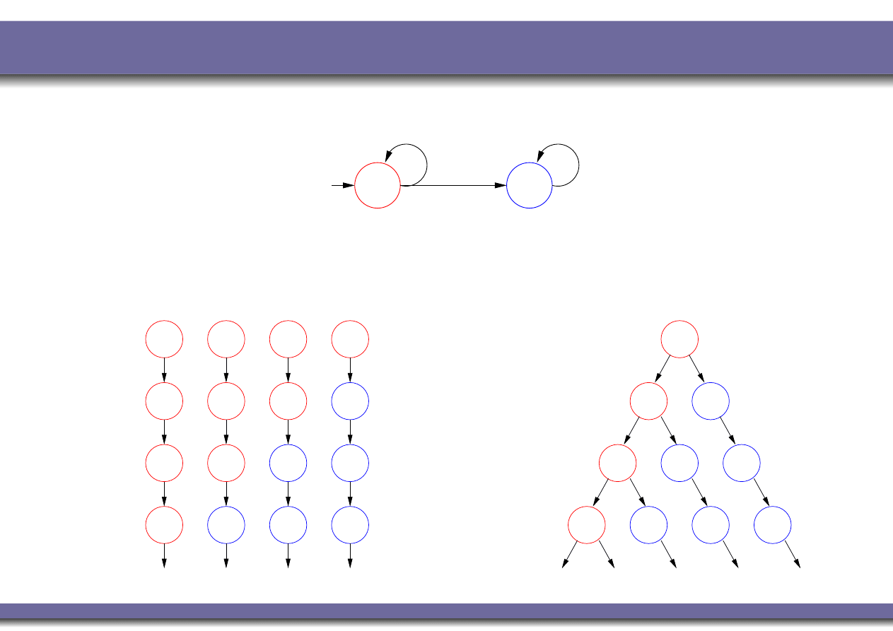
Kripke Models and Linear Structures

Consider the following Kripke structure:

done

!done

Its paths/computations can be seen as a set of linear
structures (computation tree):

done

done

done

!done

!done

!done

!done

done

done

done

!done

!done

!done

!done

!done

!done

.....

done

done

done

done

done

done

!done

!done

!done

!done

Alessandro Artale (FM – First Semester – 2009/2010) – p. 28/39

Path-Semantics for LTL

LTL formulae are evaluated over the set

N

of Natural

Numbers.

Paths in Kripke structures are infinite and linear
sequences of states. Thus, they are isomorphic to the
Natural Numbers:

π

= s

0

→ s

1

→ · · · → s

i

→ s

i

+1

→ · · ·

We want to interpret LTL formulas over Kripke
structures:

h

K M

, si |= φ

Given a Kripke structure,

K M

= (S, I, R, AP, L), a path π

in

K M

, a state s

∈ S, and an LTL formula φ, we define:

1.

h

K M

, πi |= φ

, and then

2.

h

K M

, si |= φ

Based on the LTL semantics over the Natural Numbers.

Alessandro Artale (FM – First Semester – 2009/2010) – p. 29/39

Path-Semantics for LTL (Cont.)

We first extract an

LTL model

,

M

π

= (π,

I

π

)

, from the

Kripke structure

K M

, such that:

•

π

is a path in

K M

•

I

π

is the restriction of L to states in π:

∀s ∈ π and ∀p ∈ AP, p ∈

I

π

(s) iff p ∈ L(s)

Given a Kripke structure,

K M

= (S, I, R, AP, L), a path π

in

K M

, a state s

∈ S, and an LTL formula φ:

1.

h

K M

, πi |= φ iff h

M

π

, s

0

i |= φ

with s

0

initial state of π

2.

h

K M

, si |= φ iff h

K M

, πi |= φ

for all paths π starting at s.

Alessandro Artale (FM – First Semester – 2009/2010) – p. 30/39

LTL Model Checking Definition

Given a Kripke structure,

K M

= (S, I, R, AP, L), the

LTL model

checking problem

,

K M

|= φ

:

Checks if

h

K M

, s

0

i |= φ,

for every s

0

∈ I

, initial state of

the Kripke structure

K M

Alessandro Artale (FM – First Semester – 2009/2010) – p. 31/39

Summary

Introducing Temporal Logics.

Intuitions beyond Linear Temporal Logic.

LTL: Syntax and Semantics.

LTL in Computer Science.

LTL Interpreted over Kripke Models.

LTL and Model Checking: Intuitions.

Alessandro Artale (FM – First Semester – 2009/2010) – p. 32/39

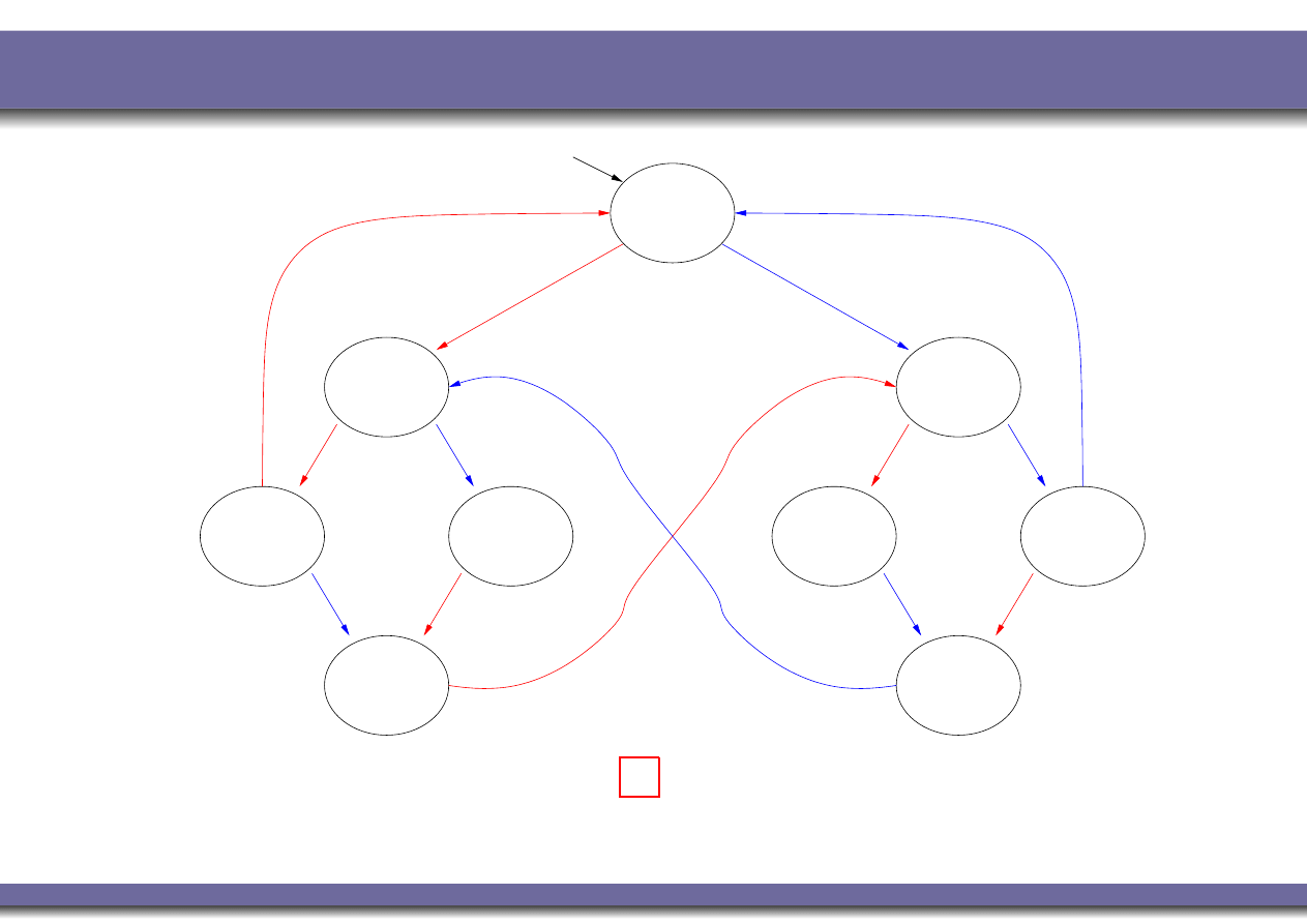
Example 1: mutual exclusion (safety)

N1, N2

turn=0

turn=1

C1, T2

turn=1

T1, T2

T1, N2

turn=1

C1, N2

turn=1

T1, T2

turn=2

N = noncritical, T = trying, C = critical

User 1

User 2

N1, T2

turn=2

T1, C2

turn=2

turn=2

N1, C2

K M

|=

¬(C

1

∧C

2

)

?

Alessandro Artale (FM – First Semester – 2009/2010) – p. 33/39

Example 1: mutual exclusion (safety)

N1, N2

turn=0

turn=1

C1, T2

turn=1

T1, T2

T1, N2

turn=1

C1, N2

turn=1

T1, T2

turn=2

N = noncritical, T = trying, C = critical

User 1

User 2

N1, T2

turn=2

T1, C2

turn=2

turn=2

N1, C2

K M

|=

¬(C

1

∧C

2

)

?

YES

: There is no reachable state in which

(C

1

∧C

2

) holds!

Alessandro Artale (FM – First Semester – 2009/2010) – p. 33/39

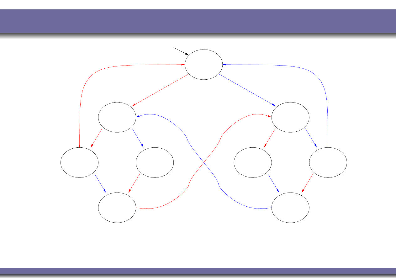
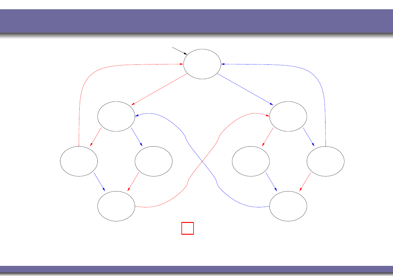
Example 2: mutual exclusion (liveness)

N1, N2

turn=0

turn=1

C1, T2

turn=1

T1, T2

T1, N2

turn=1

C1, N2

turn=1

T1, T2

turn=2

N = noncritical, T = trying, C = critical

User 1

User 2

N1, T2

turn=2

T1, C2

turn=2

turn=2

N1, C2

K M

|=

♦

C

1

?

Alessandro Artale (FM – First Semester – 2009/2010) – p. 34/39

Example 2: mutual exclusion (liveness)

N1, N2

turn=0

turn=1

C1, T2

turn=1

T1, T2

T1, N2

turn=1

C1, N2

turn=1

T1, T2

turn=2

N = noncritical, T = trying, C = critical

User 1

User 2

N1, T2

turn=2

T1, C2

turn=2

turn=2

N1, C2

K M

|=

♦

C

1

?

NO

: the blue cyclic path is a counterexample!

Alessandro Artale (FM – First Semester – 2009/2010) – p. 34/39

Example 3: mutual exclusion (liveness)

N1, N2

turn=0

turn=1

C1, T2

turn=1

T1, T2

T1, N2

turn=1

C1, N2

turn=1

T1, T2

turn=2

N = noncritical, T = trying, C = critical

User 1

User 2

N1, T2

turn=2

T1, C2

turn=2

turn=2

N1, C2

K M

|=

(T

1

⇒

♦

C

1

)

?

Alessandro Artale (FM – First Semester – 2009/2010) – p. 35/39

Example 3: mutual exclusion (liveness)

N1, N2

turn=0

turn=1

C1, T2

turn=1

T1, T2

T1, N2

turn=1

C1, N2

turn=1

T1, T2

turn=2

N = noncritical, T = trying, C = critical

User 1

User 2

N1, T2

turn=2

T1, C2

turn=2

turn=2

N1, C2

K M

|=

(T

1

⇒

♦

C

1

)

?

YES

: in every path if T

1

holds afterwards C

1

holds!

Alessandro Artale (FM – First Semester – 2009/2010) – p. 35/39

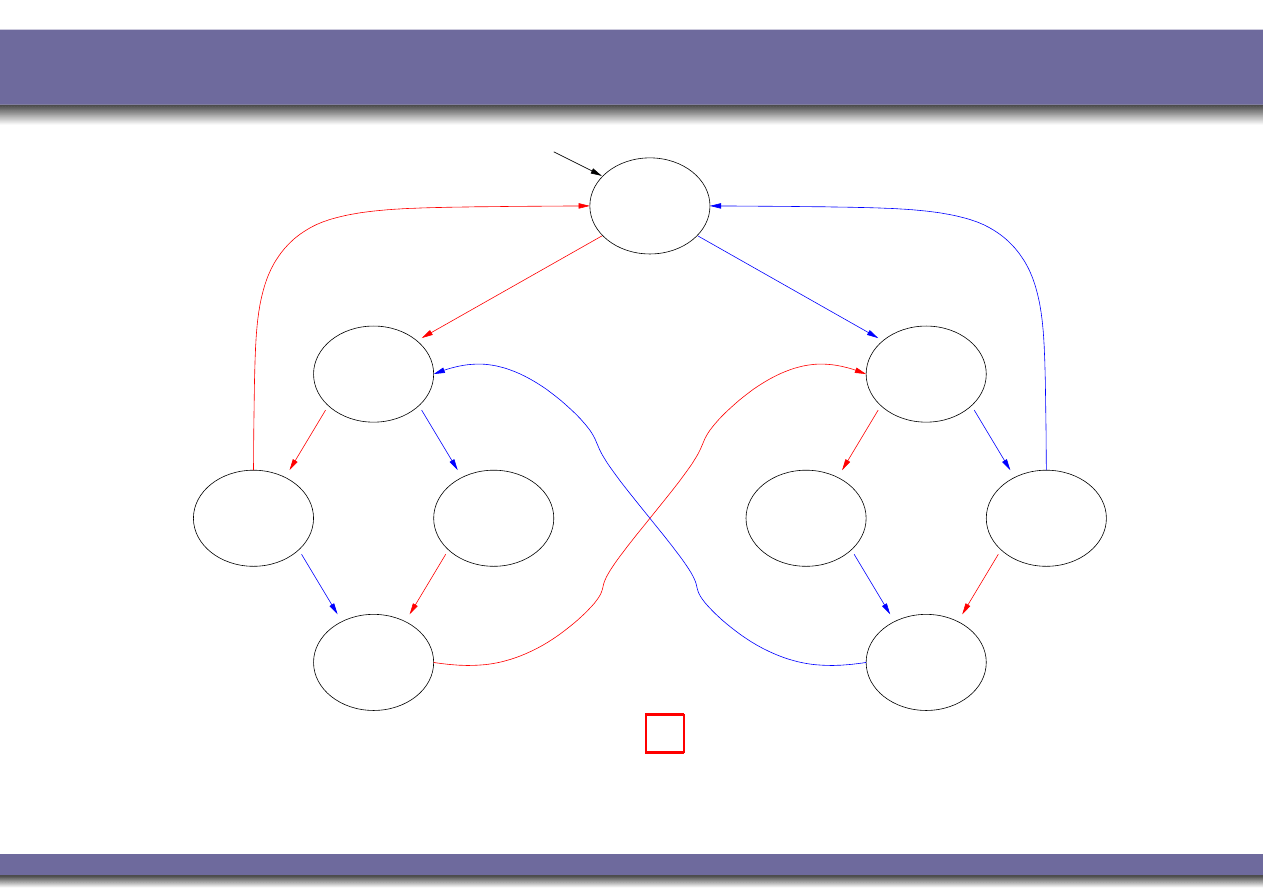
Example 4: mutual exclusion (fairness)

N1, N2

turn=0

turn=1

C1, T2

turn=1

T1, T2

T1, N2

turn=1

C1, N2

turn=1

T1, T2

turn=2

N = noncritical, T = trying, C = critical

User 1

User 2

N1, T2

turn=2

T1, C2

turn=2

turn=2

N1, C2

K M

|=

♦

C

1

?

Alessandro Artale (FM – First Semester – 2009/2010) – p. 36/39

Example 4: mutual exclusion (fairness)

N1, N2

turn=0

turn=1

C1, T2

turn=1

T1, T2

T1, N2

turn=1

C1, N2

turn=1

T1, T2

turn=2

N = noncritical, T = trying, C = critical

User 1

User 2

N1, T2

turn=2

T1, C2

turn=2

turn=2

N1, C2

K M

|=

♦

C

1

?

NO

: the blue cyclic path is a counterexample!

Alessandro Artale (FM – First Semester – 2009/2010) – p. 36/39

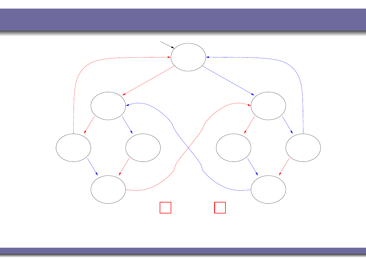
Example 4: mutual exclusion (strong fairness)

N1, N2

turn=0

turn=1

C1, T2

turn=1

T1, T2

T1, N2

turn=1

C1, N2

turn=1

T1, T2

turn=2

N = noncritical, T = trying, C = critical

User 1

User 2

N1, T2

turn=2

T1, C2

turn=2

turn=2

N1, C2

K M

|=

♦

T

1

⇒

♦

C

1

?

Alessandro Artale (FM – First Semester – 2009/2010) – p. 37/39

Example 4: mutual exclusion (strong fairness)

N1, N2

turn=0

turn=1

C1, T2

turn=1

T1, T2

T1, N2

turn=1

C1, N2

turn=1

T1, T2

turn=2

N = noncritical, T = trying, C = critical

User 1

User 2

N1, T2

turn=2

T1, C2

turn=2

turn=2

N1, C2

K M

|=

♦

T

1

⇒

♦

C

1

?

YES

: every path which visits T

1

infinitely often also visits C

1

infinitely often!

Alessandro Artale (FM – First Semester – 2009/2010) – p. 37/39

LTL Alternative Notation

Alternative notations are used for temporal operators.

♦

F

sometime in the

F

uture

G

G

lobally in the future

k

X

ne

X

time

Alessandro Artale (FM – First Semester – 2009/2010) – p. 38/39

Summary of Lecture III

Introducing Temporal Logics.

Intuitions beyond Linear Temporal Logic.

LTL: Syntax and Semantics.

LTL in Computer Science.

LTL Interpreted over Kripke Models.

LTL and Model Checking: Intuitions.

Alessandro Artale (FM – First Semester – 2009/2010) – p. 39/39