
Rate of heat conduction
in a specified direction:
- proportional to the temperature gradient
- three-dimensional (3D)
Heat conduction
in a medium:
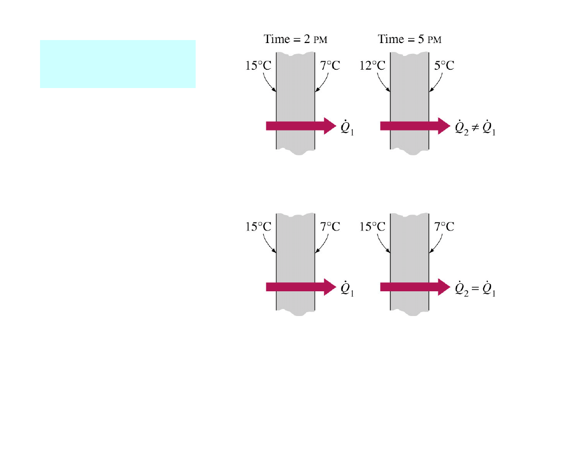
- steady (T = const with time at any point within the
medium) or unsteady (transient) (T≠
≠
≠
≠ const)
- one-dimensional (when conduction is significant only
in 1D) or 2D / 3D
Heat transfer
has direction and magnitude
→
→
→
→
vector character
HEAT TRANSFER – HEAT CONDUCTION EQUATION
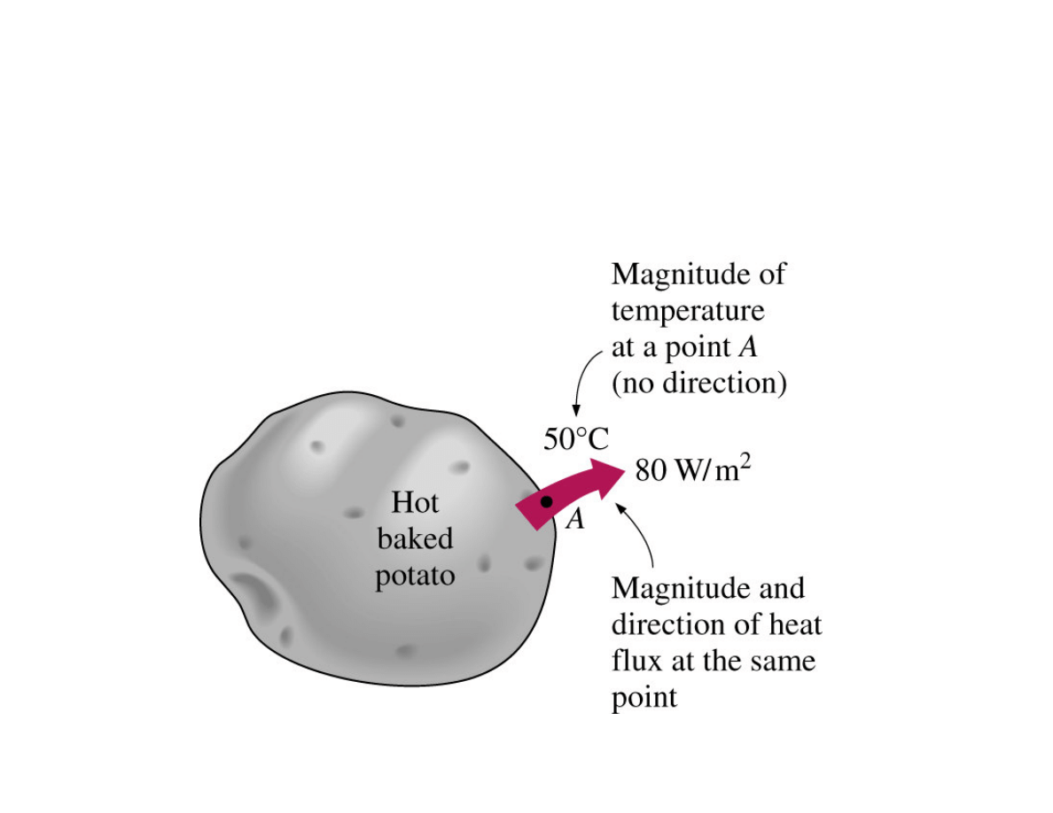
Heat transfer has vector features →
→
→
→ direction and
magnitude at a point.
Temperature is a scalar quantity.
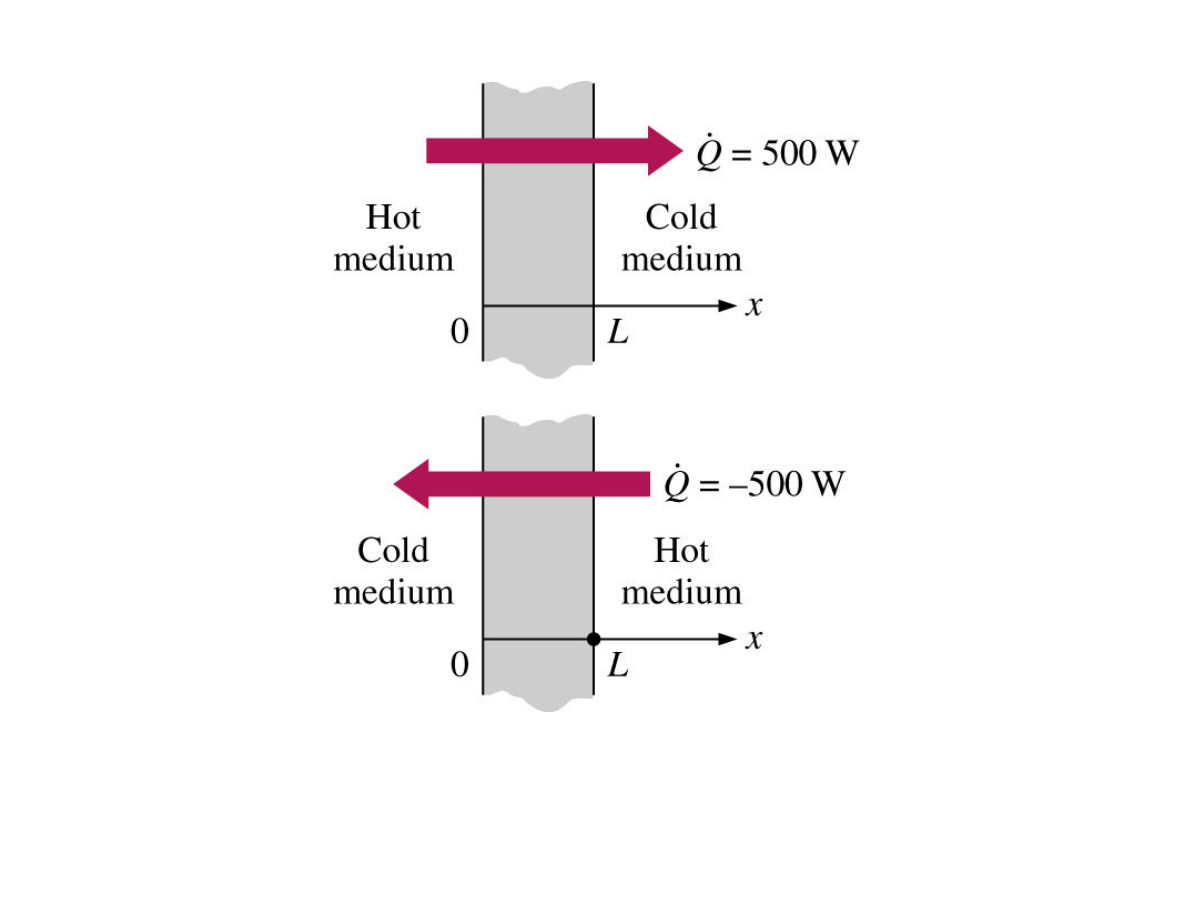
Indicating directions for heat transfer rate:
- positive (negative) in the positive (negative) x direction
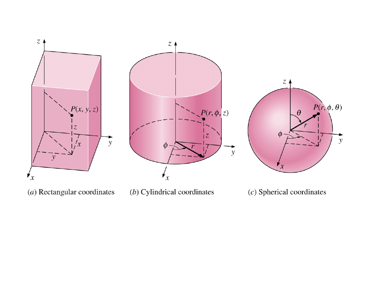
Different coordinate systems for describing the location
of a point P
(a)
Transient (real) and
(b)
steady (often used in modelling) heat
conduction
→
→
→
→ usual assumption in the case of a typical house:
-
maximum
rate of heat loss under
worst
conditions for an
extended period of time.
(b) Steady-state
(a) Transient
1D heat transfer
in a plane wall
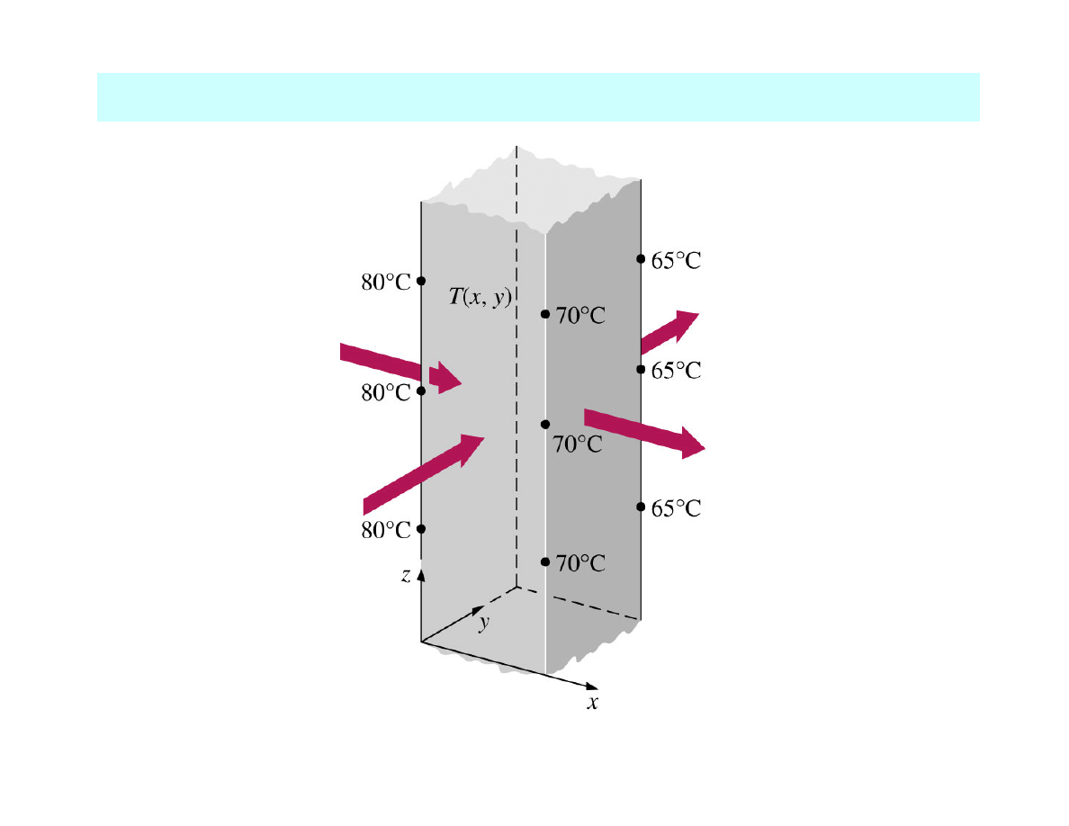
2D heat transfer in a long rectangular bar
MULTIDIMENSIONAL HEAT TRANSFER
x
Q
•
y
Q
•
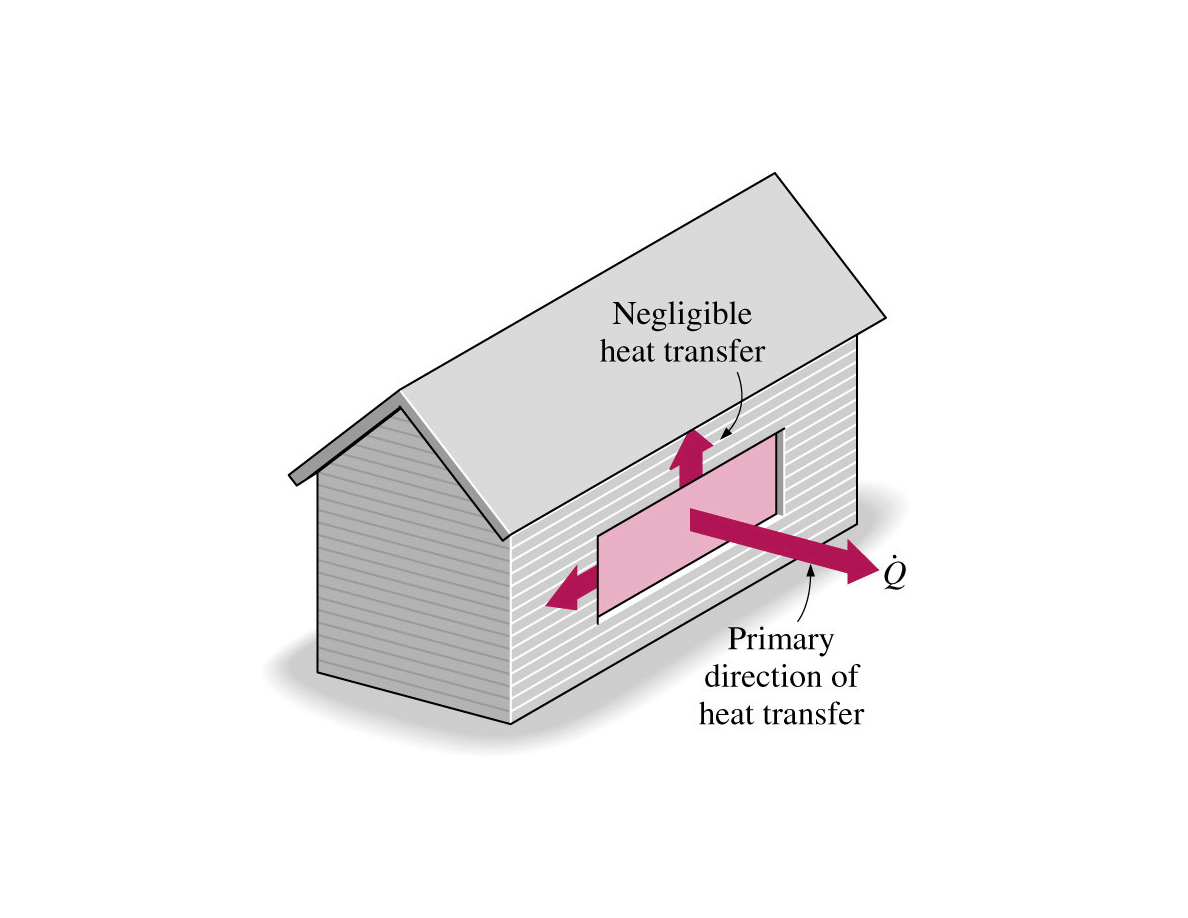
1D heat transfer through the window of a house
In practice – 3D heat transfer often simplified to 1D case
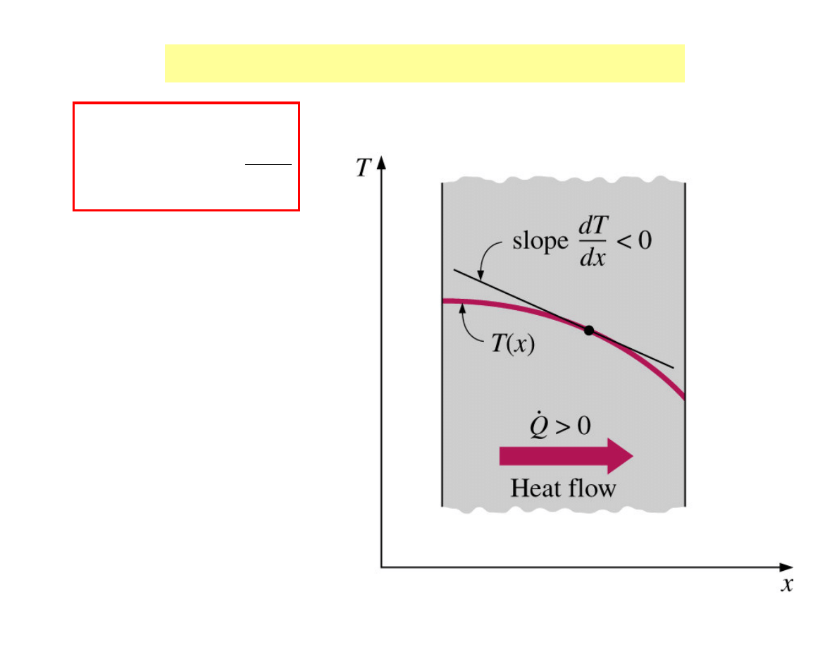
1D Fourier`s law of heat conduction
dx
dT
A
Q
Λ
−
=
•
(W)
where:
Λ
Λ
Λ
Λ
- thermal conductivity
of the material
dT/dx
- temperature
gradient
→
→
→
→ slope of the
temperature curve on
the T-x diagram
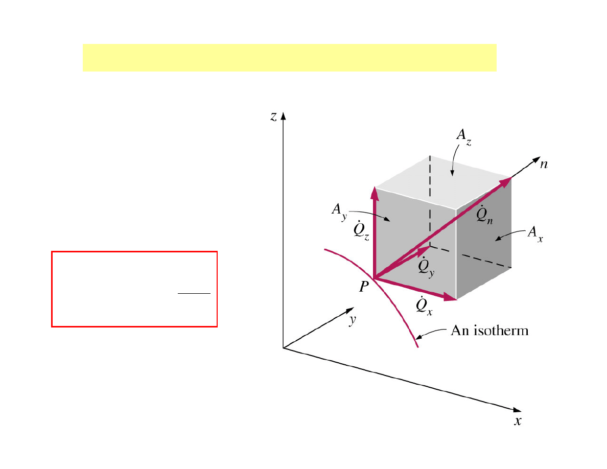
3D Fourier`s law of heat transfer at point P
Isothermal surface with
a normal heat transfer
vector
n
Q
•
n - direction of decreasing T
n
T
A
n
Q
∂
∂
Λ
−
=
•
(W)
In rectangular coordinates, the heat conduction vector:
k
z
j
y
i
x
n
Q
Q
Q
Q
r
r
r
•
•
•
•
+
+
=
where - i, j, k are the unit vectors
z
y
x
Q
Q
Q
•
•
•
,
,
are the magnitudes of heat transfer rates
in the x-, y- and z-directions, which can
be determined from Fourier`s law as:
dy
dT
A
y
y
Q
Λ
−
=
•
dz
dT
A
z
z
Q
Λ
−
=
•
dx
dT
A
x
x
Q
Λ
−
=
•
where A
x
, A
y
, A
z
are heat conduction areas normal to the
x-, y- and z-directions, respectively.
For isotropic materials: A
x
= A
y
= A
z
For anisotropic materials: A
x
≠
≠
≠
≠
A
y
≠
≠
≠
≠
A
z

HEAT GENERATION
- Conversion of electrical, chemical, or nuclear energy
into heat (or thermal) energy in solid
• Resistance wire →
→
→
→ electrical energy generation
of heat at a rate of
I
2
R
,
where:
I
- current
R
- electrical resistance of the wire
→
→
→
→ electronic cooling
• Exothermic chemical reactions →
→
→
→ heat source
Endothermic chemical reactions
→
→
→
→ heat sink
• Fuel elements of nuclear reactors →
→
→
→ nuclear fission
→
→
→
→ heat source for the nuclear power plants
Sun
→
→
→
→ nuclear reactor (fusion of hydrogen to helium)
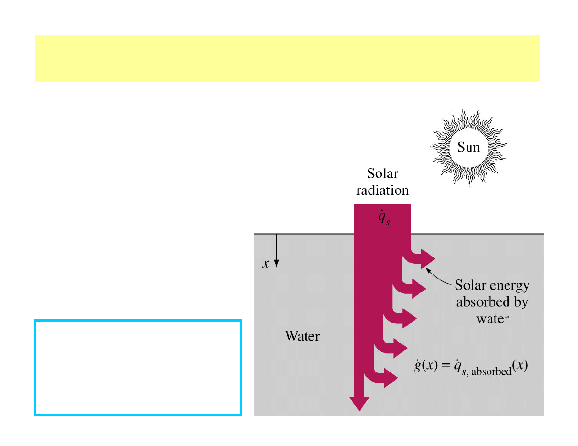
Modelling of absorption of radiation (solar energy or
gamma rays) →
→
→
→
heat generation
Heat generation - volumetric phenomenon
Thus the heat generation rate
- specified
per unit volume
in W / m
3
g
•
Total rate of heat generation
in a medium of volume V
can be determined from
dV
V
g
G ∫
=
•
•
In the case of uniform
heat generation:
V
g
G
•
•
=
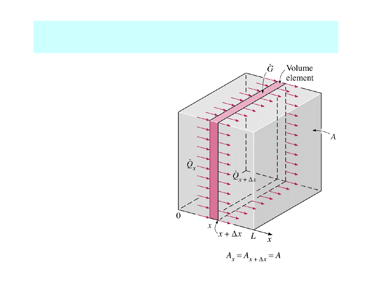
ONE-DIMENSIONAL HEAT CONDUCTION EQUATION
in a large plane wall
∆
∆
∆
∆x – thickness
ρ
ρ
ρ
ρ - material density
C - specific heat
A - area normal to
the direction of
heat transfer
We consider a thin volume element
with the parameters:
Energy balance
for the thin element during
a small time interval
∆
∆
∆
∆t
Rate of heat
conduction
at x
Rate of heat
conduction
at x+∆
∆
∆
∆x
Rate of heat
generation
inside the
element
Rate of change
of the energy
content of the
element
_
+
=
t
E
x
x
x
G
Q
Q
∆
∆
=
+
∆
+
−
•
•
•
or:
x
A
V
T
T
x
CA
T
T
mC
E
E
E
g
g
G
t
t
t
t
t
t
t
t
t
∆
=
=
−
∆
=
−
=
−
=
∆
•
•
•
∆
+
∆
+
∆
+
)
(
)
(
ρ
After substitution and division by A
∆
∆
∆
∆
x:
t
T
T
C
x
x
x
x
A
t
t
t
g
Q
Q
∆
−
=
+
∆
−
∆
+
−
∆
+
•
•
•
ρ
1
In the limit ∆
∆
∆
∆x →
→
→
→ 0 and ∆
∆
∆
∆t →
→
→
→ 0:
From Fourier`s law
∂
∂
Λ
−
∂
∂
=
∂
∂
=
∆
−
∆
+
•
•
•
→
∆
x
T
A
x
x
x
x
x
x
Q
Q
Q
x
lim
0
Thus:
t
T
C
x
T
A
x
A
g
∂
∂
=
+
∂
∂
Λ
∂
∂
•
ρ
1
Since A = const, for
variable conductivity
Λ
Λ
Λ
Λ:
t
T
C
x
T
x
g
∂
∂
=
+
∂
∂
Λ
∂
∂
•
ρ
- differential
equation with
2 variables (x and t)
Assumption in most practical applications:
Λ
Λ
Λ
Λ = const
Thus:
t
T
x
T
g
∂
∂
=
Λ
+
∂
∂
•
α
1
2
2
Under special conditions:
(1) Steady-state (∂
∂∂
∂/∂
∂∂
∂t = 0):
0
2
2
=
Λ
+
•
g
x
d
T
d
(2) Transient, no net
generation (g = 0):
t
T
x
T
∂
∂
=
∂
∂
α
1
2
2
0
2
2
=
x
d
T
d
(3) Steady-state, no heat
generation (∂
∂∂
∂/∂
∂∂
∂t = 0 and g = 0):
where:
α
α
α
α = Λ
Λ
Λ
Λ/(ρ
ρ
ρ
ρC)
-
thermal diffusivity
)
/
(
2
s
m
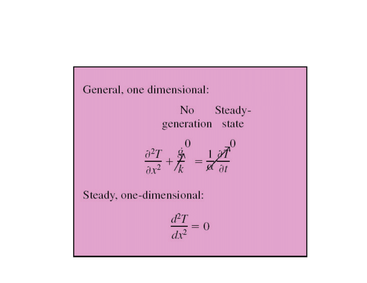
Summary: Simplification of the 1D heat conduction equation
in a
plane wall
for the case of constant conductivity for
steady conduction with no heat generation:
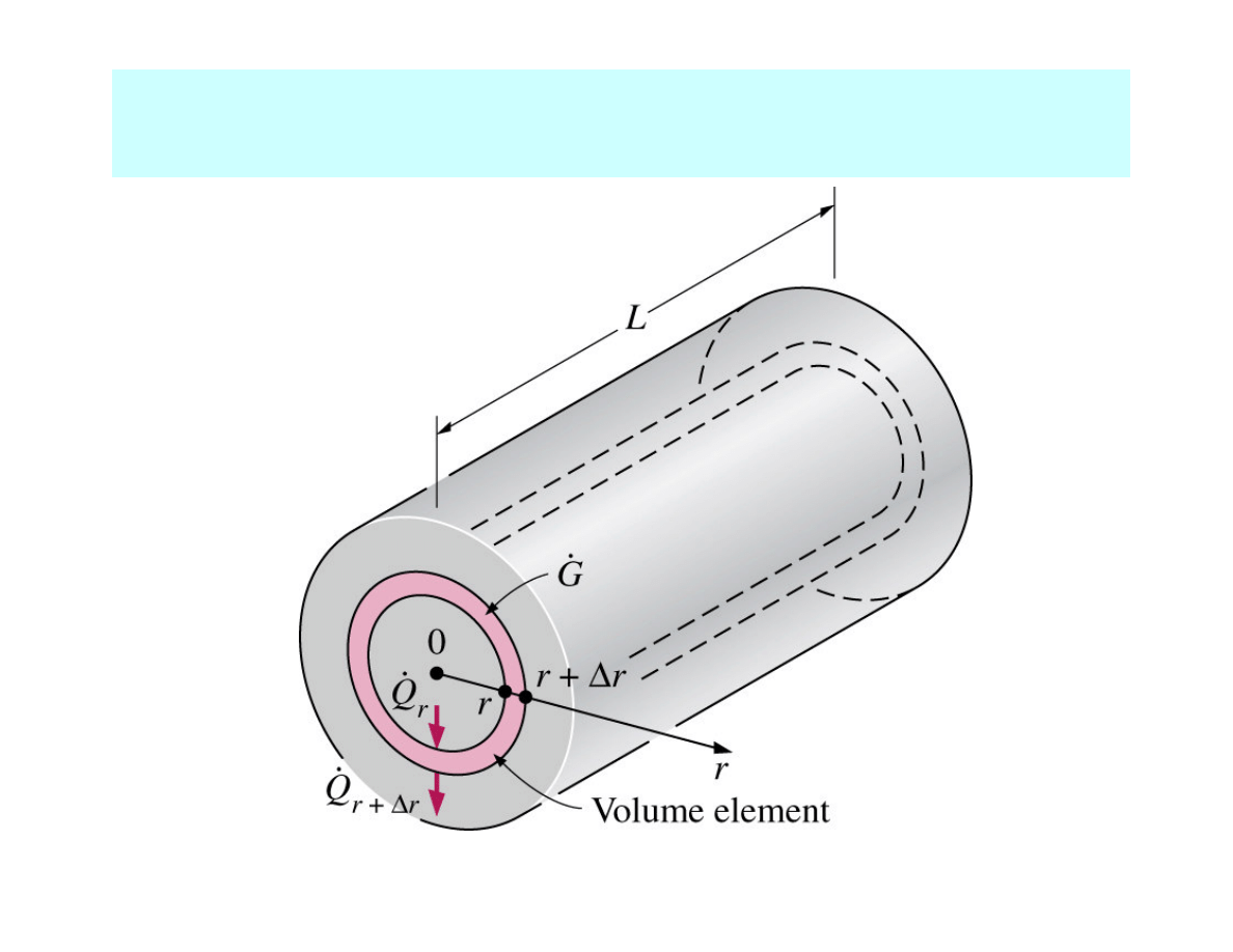
HEAT CONDUCTION EQUATION
in a long cylinder
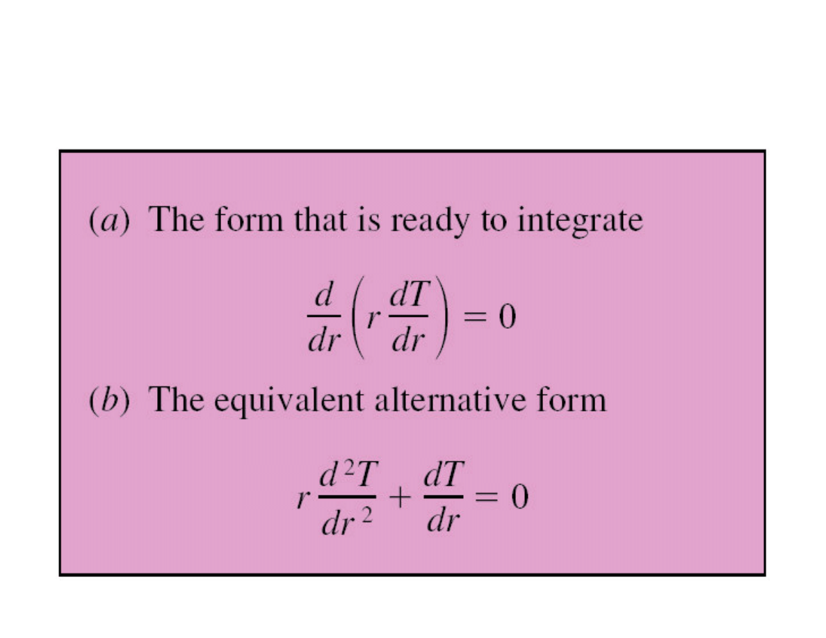
1D steady heat conduction equation (variable r) in
a
cylinder
with no heat generation:
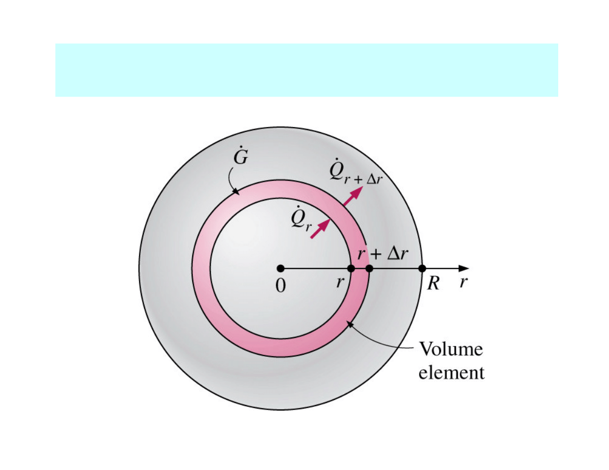
HEAT CONDUCTION EQUATION
in a sphere

1D steady heat conduction equation (variable r) in
a
sphere
with no heat generation:
2
2

t
T
C
r
T
r
r
r
g
n
n
∂
∂
=
+
∂
∂
Λ
∂
∂
•
ρ
1
COMBINED 1D HEAT CONDUCTION EQUATION
where:
n = 0 for a plane wall
n = 1 for a cylinder
n = 2 for a sphere
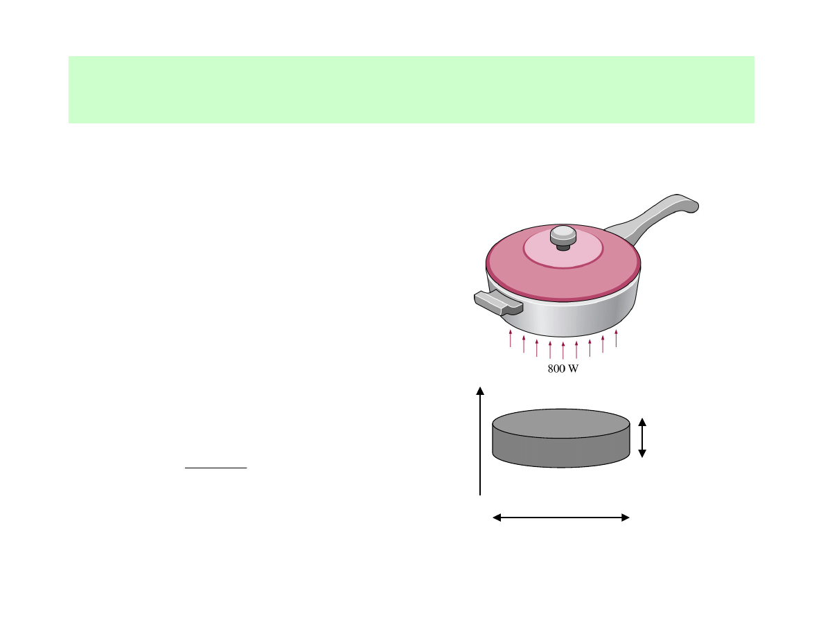
Example: Modelling of the heat conduction through the
bottom of a pan
• Assumption of the large plane wall,
because
Thus:
1D steady heat conduction
equation with no heat
generation:
D = 18 cm
L = 4 cm
x
0
2
2
=
x
d
T
d
L<<
<<
<<
<< D
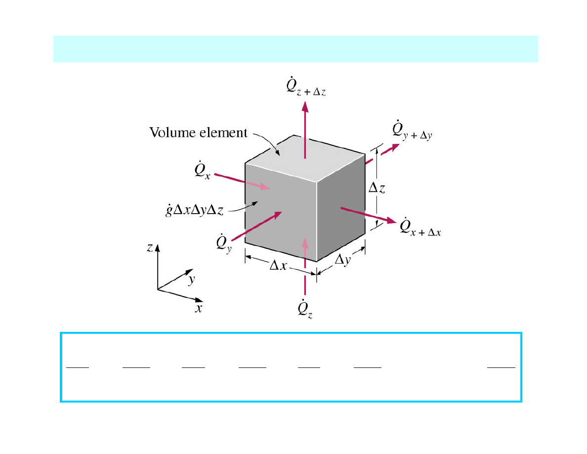
GENERAL 3D HEAT CONDUCTION EQUATION
t
T
C
z
T
z
y
T
y
x
T
x
g
∂
∂
=
+
∂
∂
Λ
∂
∂
+
∂
∂
Λ
∂
∂
+
∂
∂
Λ
∂
∂
•
ρ

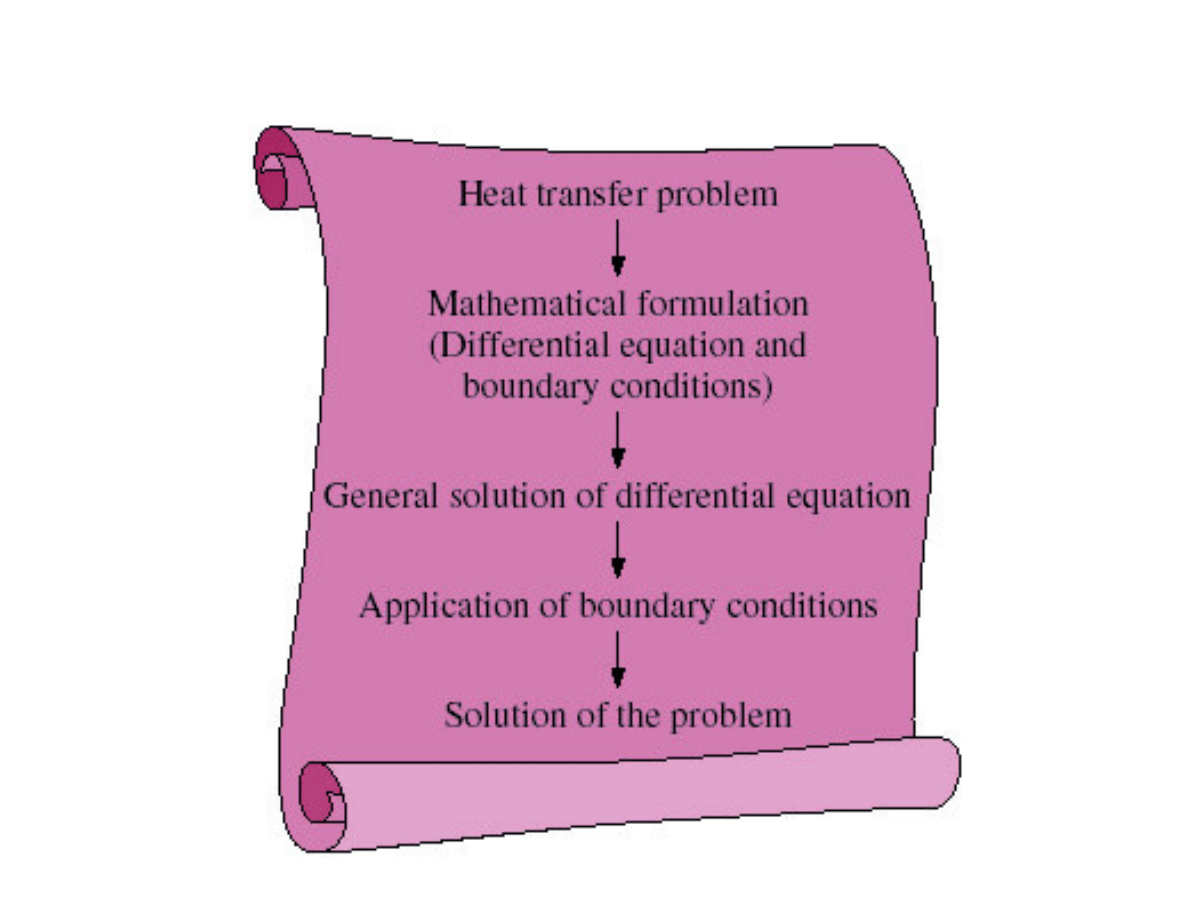
BOUNDARY AND INITIAL CONDITIONS
• Heat transfer in a medium depends on the surface
thermal conditions →
→
→
→ importance of
boundary and initial
conditions
for a unique solution of a differential equation
• Solving a differential equation →
→
→
→ removing derivatives
(integration)
→
→
→
→ introducing arbitrary constants
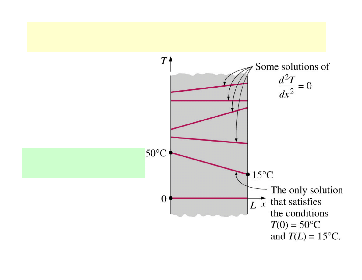
Example: steady heat flux
0
2
2
=
x
d
T
d
General solution:
2
1
)
(
C
x
C
x
T
+
=
where C
1
and C
2
are arbitrary constants
• Some specific solutions:
3
)
(
12
)
(
5
2
)
(
−
=
+
−
=
+
=
x
T
x
x
T
x
x
T
Problem: Distribution of T along the brick wall
→
→
→
→ dependence on conditions at the two surfaces:
- air temperature of
the house
- velocity and direction
of the wind (convection)
- solar energy incident
on the outer surface
(radiation)
Solving the heat
conduction equation:
•
Steady heat flow
→
→
→
→
boundary conditions
:
T(x=0, t) and T(x=L, t)
•
Unsteady flow
→
→
→
→ boundary conditions
and
initial conditions
: T(x, y, z, t = 0)
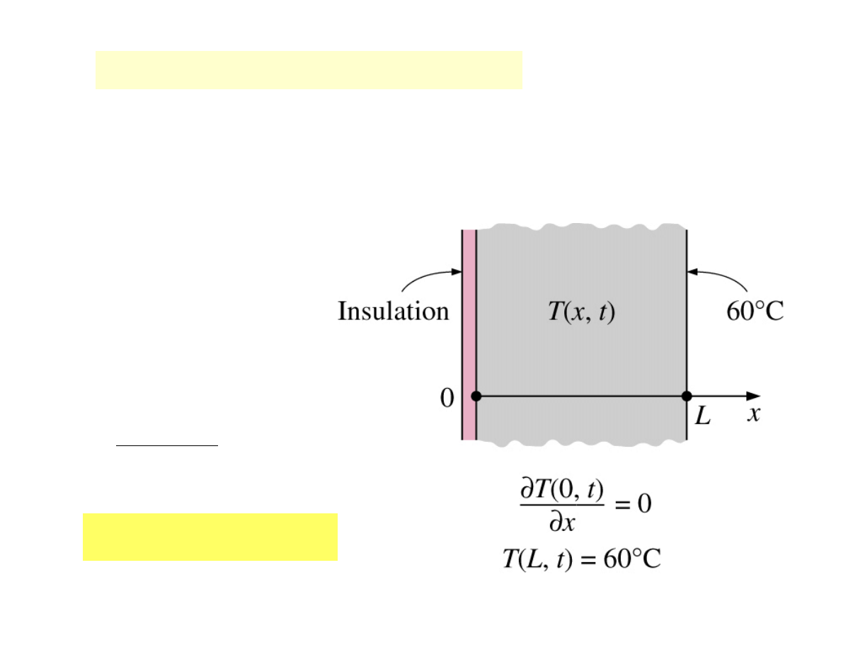
Special case
: Insulated boundary
Insulation
- reducing heat transfer through the wall to
the negligible level
0
=
•
q
Thus:
0
)
,
0
(
=
∂
∂
Λ
x
t
T
const
t
x
T
=
⇒
)
,
(
Problem: Temperature distribution in the wall

Superinsulations
- by using layers of highly reflective sheets
separated by glass fibers in an evacuated space.
Radiation heat transfer between two surfaces is inversely proportional
to the number of sheets used and thus heat loss by radiation will be
very low by using this highly reflective sheets.
At the same time, evacuating the space between the layers forms a
vacuum under 0.000001 atm pressure which minimize conduction or
convection through the air space between the layers.
Technology of insulation
Ordinary insulations
- by mixing fibers, powders, or flakes of
insulating materials with air.
Heat transfer through such insulations is by conduction through
the solid material, and conduction or convection through the air
space as well as radiation.
Such systems are characterized by
apparent thermal conductivity
instead of the ordinary thermal conductivity in order to incorporate
these convection and radiation effects.
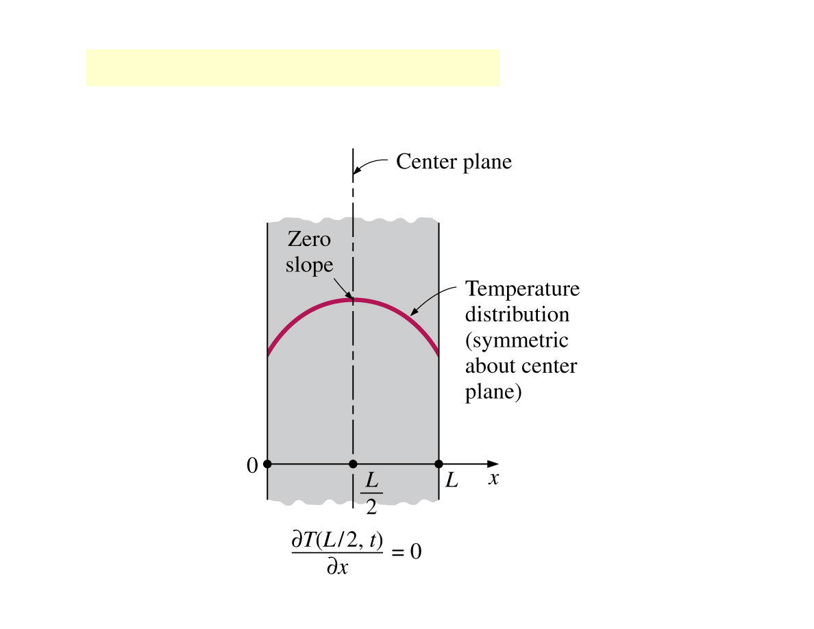
Special case
: Thermal symmetry
Example: hot plate of thickness L suspended in air
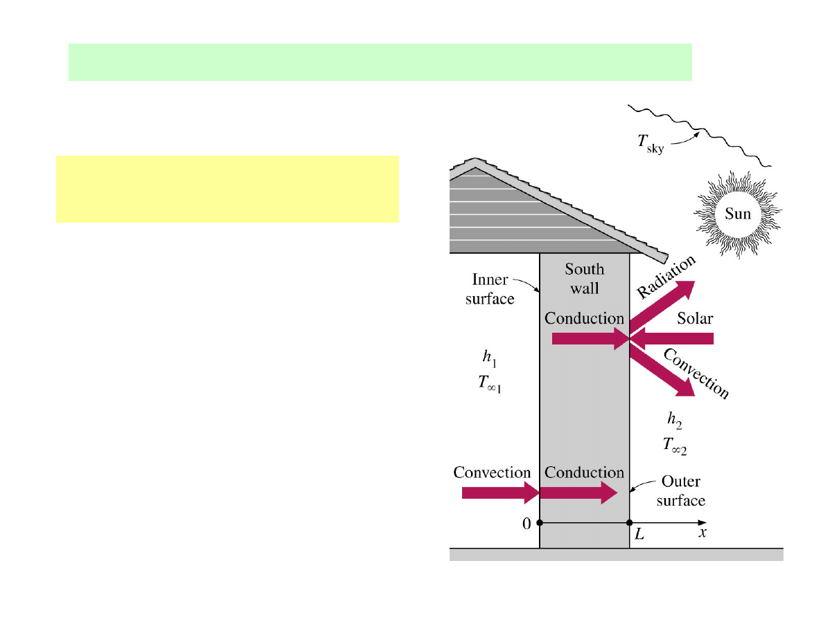
Combined convection, radiation and heat flux
Example:
The south wall of a house
Data for quantitative modelling
:
L=0.2 m
α
α
α
α = 0.5 - absorptivity for solar energy
T
∞
∞
∞
∞1
= 20
o
C, T
∞
∞
∞
∞1
= 5
o
C
T
sky
= 255 K
h
1
=6 W/(m
2
·
o
C), h
2
= 25 W/(m
2
·
o
C) - convection
coefficients (inner and outer surfaces)
Λ
Λ
Λ
Λ = 0.7 W/(m
o
C)
εεεε
2
= 0.9 - emmisivity of the outer surface
Assumption:
1D steady heat transfer

solar
T
L
T
T
L
T
h
dx
L
dT
q
ky
•
∞
−
−
+
−
=
Λ
−
α
σ
ε
]
)
(
[
]
)
(
[
)
(
4
4
2
2
2
- outer - convection, radiation and heat flux
Modelling: T = T(x)
Boundary conditions
:
- inner - only convection
)]
0
(
[
)
0
(
1
1
T
T
h
dx
dT
−
=
Λ
−
∞
SUMMARY
Wyszukiwarka
Podobne podstrony:
09 Transient heat conduction
EŚT 07 Użytkowanie środków transportu
07 Windows
07 MOTYWACJAid 6731 ppt
Planowanie strategiczne i operac Konferencja AWF 18 X 07
Wyklad 2 TM 07 03 09
ankieta 07 08
Szkol Okres Pracodawcy 07 Koszty wypadków
Wyk 07 Osprz t Koparki
zarządzanie projektem pkt 07
Prezentacja NFIN 07
więcej podobnych podstron